A Tsunami in LisbonWhere to run?

Daniel A. S. CondeUnder the supervision of Professor Rui M. L. Ferreira

October 15, 2012

1 Introduction

Tsunamis are waveforms mostly originated by the vertical displacement of the seafloor as a con-

sequence of an earthquake, internal or external landslides, or volcanic eruptions. They propagate

in the ocean as long waves carrying a large amount of kinetic energy. In deep waters, they ex-

hibit low amplitude, relatively to the mean local sea level, which makes them difficult to observe

directly. As they travel up the continental slope, the wavelength typically reduces and the am-

plitude increases. The name tsunami, loosely translated as harbour waves, addresses the fact

that the wave becomes visible only after shoaling. Approaching shore, the waves may break and

form bores that propagate overland (Yeh, 1991). At this stage the tsunami becomes particularly

destructive as its great momentum is imparted to the obstacles it encounters. It incorporates

debris, either natural sediment eroded from the bottom boundary or remains of human built

environment, as seen in the recent 2004 and 2011 occurrences in Sumatra and Japan.

A recent revision of the catalogue of tsunamis in Portugal has shown that Tagus estuary has

been affected by catastrophic tsunamis numerous times over the past two millennia (Baptista &

Miranda, 2009). This justifies the modelling efforts aimed at quantifying potential inundation

areas for present-day altimetry and bathymetry of Tagus estuary. Such modelling efforts have

been undertaken recently Baptista et al. (2006) but improvements can be achieved both in

conceptual model and discretization techniques.

The objectives of this work are: i) to present a 2DH mathematical model applicable to discon-

tinuous flows over complex geometries, such as tsunami propagation overland, ii) to adapt and

apply the model to the propagation of a 1755-like tsunami in the Tagus estuary and iii) to assess

the exposure of the Tagus estuary riverfront. The model is based on conservation equations of

mass and momentum of water and granular material, derived within the shallow flow hypothesis,

constituting a hyperbolic system of conservation laws. It features non-equilibrium sediment trans-

port, conceived as an imbalance between capacity and actual bedload discharge. Flow friction,

capacity bedload discharge and the characteristic length describing return-to-capacity require

closure equations (Ferreira et al., 2009). This conceptual approach allows for the description of

a tsunami once it has incorporated debris and interacts with bed morphology.

1

Particularly robust numerical discretization techniques within the Finite-Volume framework have

been developed by Murillo & García-Navarro (2010) allowing for fully conservative solutions

to initial value problems (IVPs). Finite-volume techniques are compatible with body-fitting

unstructured meshes. This allows for optimization of computational effort, since the domain

can be discretized with large cells, where flow gradients are small, and with small cells in the

vicinity of flow obstacles (such as buildings) and, in general, where flow gradients are expected

to be large. This requires good articulation of numerical discretization with GIS tools, an issue

addressed with care in the present work.

2 Conceptual Model

2.1 Governing Equations

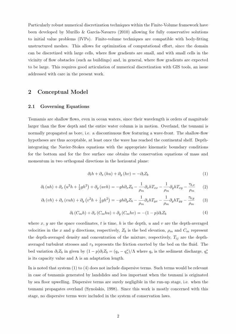
Tsunamis are shallow flows, even in ocean waters, since their wavelength is orders of magnitude

larger than the flow depth and the entire water column is in motion. Overland, the tsunami is

normally propagated as bore, i.e. a discontinuous flow featuring a wave-front. The shallow-flow

hypotheses are thus acceptable, at least once the wave has reached the continental shelf. Depth-

integrating the Navier-Stokes equations with the appropriate kinematic boundary conditions

for the bottom and for the free surface one obtains the conservation equations of mass and

momentum in two orthogonal directions in the horizontal plane:

∂th+ ∂x (hu) + ∂y (hv) = −∂tZb (1)

∂t (uh) + ∂x(u2h+ 1

2gh2)

+ ∂y (uvh) = −gh∂xZb −1

ρm∂xhTxx −

1

ρm∂yhTxy −

τb,xρm

(2)

∂t (vh) + ∂x (vuh) + ∂y(v2h+ 1

2gh2)

= −gh∂yZb −1

ρm∂xhTyx −

1

ρm∂yhTyy −

τb,yρm

(3)

∂t (Cmh) + ∂x (Cmhu) + ∂y (Cmhv) = −(1− p)∂tZb (4)

where x, y are the space coordinates, t is time, h is the depth, u and v are the depth-averaged

velocities in the x and y directions, respectively, Zb is the bed elevation, ρm and Cm represent

the depth-averaged density and concentration of the mixture, respectively, Tij are the depth-

averaged turbulent stresses and τ b represents the friction exerted by the bed on the fluid. The

bed variation ∂tZb in given by (1− p)∂tZb = (qs − q∗s)/Λ where qs is the sediment discharge, q∗sis its capacity value and Λ is an adaptation length.

In is noted that system (1) to (4) does not include dispersive terms. Such terms would be relevant

in case of tsunamis generated by landslides and less important when the tsunami is originated

by sea floor upwelling. Dispersive terms are surely negligible in the run-up stage, i.e. when the

tsunami propagates overland (Synolakis, 1998). Since this work is mostly concerned with this

stage, no dispersive terms were included in the system of conservation laws.

2

2.2 Closure Models

The proposed system of governing equations requires closures for the dynamics of the bedload

layer, the evolution of bed morphology and finally for flow resistance, τb and Tij (Ferreira et al.,

2009). The bed shear stress is given by,

τb,i = Cfρ‖|u|‖ui (5)

where the friction coeficient, Cf , can be given by the Manning-Strickler formula, Cf = g/(h1/3K2

)where K is Strickler’s coefficient whose dimensions are L1/3T−1, or by the formula proposed by

Ferreira et al. (2009) if the wave carries debris. The turbulent stress tensor is given by,

Tij = ρνT(∂xjui + ∂xiuj

)(6)

where the eddy viscosity, νT , is expressed by the a simplified zero-equation κ − ε model (Pope,

2000).

Several bedload formulas can be used to describe capacity bedload transport, among them the

well-known Meyer-Peter & Müller, 1947, and Bagnold, 1966, formulas (S.Yalin, 1977). A specific

formula for stratified flows (sheet flow) and debris flow is also incorporated. The bedload dis-

charge is defined as q∗s = C∗c |uc|hc where C∗c and uc are the layer-averaged capacity concentration

and velocity, respectively, in the contact load layer. Assuming that the thickness of the contact

load layer, hc, is related to the flux of kinetic energy associated to the fluctuating motion of

transported grains (Ferreira et al., 2009), one has,

hcds

= m1 +m2θ (7)

where ds is the significant particle diameter, m1 and m2 are parameters that are dependent upon

the mechanical properties of the particles and fluid viscosity and lastly θ is the Shield’s parameter,

calculated as θ = Cf‖~u‖2/ (gds(s− 1)) where Cf is the friction coefficient. The bedload layer

depth-averaged velocity, U2, is given by a power law (Ferreira, 2005),

uc = u

(hch

)1/6

(8)

The capacity concentration, C∗c , was also derived by Ferreira et al. (2009) assuming equilibrium

of the frictional sub-layer. One obtains,

C∗c =θ

tan(ϕ) (m1 +m2θ)(9)

where tan(ϕ) is the dynamic friction angle of the granular material (Bagnold, 1954).

3

3 Discretization Technique

The hyperbolic, non-homogeneous, first order, quasi-linear system of conservation laws, equations

(1) to (4), can be written in compact notation as,

∂tU(V ) +∇ ·E(U) = H(U)⇔ ∂tU(V ) + ∂xF (U) + ∂yG(U) = H(U) (10)

where the dependant non-conservative variables, V , dependant conservative variables U and

fluxes F and G are defined as,

V =

h

u

v

Cm

; U =

h

uh

vh

Cmh

; F =

uh

u2h+ 12gh

2

uvh

Cmhu

; G =

vh

vuh

v2h+ 12gh

2

Cmhv

(11)

and the source term vector H is H = R+T, where R is the parcel of source terms not susceptible

to be treated as non-conservative fluxes and T are non-physical fluxes. These terms are treated

as fluxes in order to obtain a well-balanced numerical scheme (Vázquez-Cedón, 1999) and are

defined as,

R =

− (D−E)

1−p

− τb,xρ(w)

− τb,yρ(w)

−(D − E))

; T =

0

−gh∂xZb−gh∂yZb

0

. (12)

Terms with gh∂xiZb are not physical fluxes; they are treated as so to obtain a well-balanced

numerical scheme (Vázquez-Cedón, 1999).

Employing Godunov’s finite-volume approach (Leveque, 2002), discretization, the system (3.1)

is integrated in a cell i. The following explicit flux-based finite-volume scheme is obtained,

Un+1i = Un

i −∆t

Ai

3∑k=1

Lk

4∑n=1

(λ(n)α(n) − β(n)

)−ike

(n)ik + ∆t

(Tn+1i

)(13)

where ∆t is the time step, obeying a Courant condition (CFL < 1), Ai is the cell area, Lk is

the edge length, and e(n) and e(n) are the m − th approximate eigenvectors and eigenvalues,

respectively, defined as (Roe, 1981),

λ(1)ik = (u · n− c)ik; λ

(2)ik = (u · n)ik; λ

(3)ik = (u · n + c)ik; λ

(4)ik = (u · n)ik (14)

e(1)ik =

1

u− cnxv − cnyCm

ik

; e(2)ik =

0

−cnycnx

0

ik

; e(3)ik =

1

u+ cnx

v + cny

Cm

ik

; e(4)ik =

0

0

0

1

ik

(15)

4

where coefficients α(n)ik are the wave-strengths for each of the eigenvectors and u, v, c and Cm are

the approximate values for the two velocity components, (u, v), free-surface disturbance celerity,

c, and sediment concentration, Cm, respectively. The eigenvector wave-strengths α(n)ik are given

by,

α(1)ik = ∆ik〈h〉

2 − 12cik

(∆ik 〈uh〉 − uik∆ik 〈h〉) · nikα

(2)ik = 1

cik(∆ik 〈uh〉 − uik∆ik 〈h〉) · tik

α(3)ik = ∆ik〈h〉

2 + 12cik

(∆ik 〈uh〉 − uik∆ik 〈h〉) · nikα

(4)ik = ∆ik 〈hCm〉 − Cm∆ik 〈h〉

(16)

and the approximate values of u, v, c and Cm are defined as, (Toro, 2001)

uik =ui√hi + uj

√hj√

hi +√hj

; vik =vi√hi + vj

√hj√

hi +√hj

; cik =

√ghi + hj

2; Cmik

=Cmi

√hi + Cmj

√hj√

hi +√hj(17)

The wave-strengths associated with the eigenvalues are given by,

β(1)ik = − 1

2cik

(pbρw

); β

(2)ik = 0; β

(3)ik = −β(1)

ik ; β(4)ik = 0 (18)

Only the negative part of the eigenvalues λ(m)ik and of β(m)

ik coefficients are used, ensuring that

only incoming fluxes are used in the update of the conserved variables. The shear-rate in the

definition of the depth averaged turbulent stresses, equation (2.5), is calculated from directional

derivatives. The discretized directional derivative ∇abF , of a generic differentiable variable, in

the direction of the vector rba that connects the barycentres of cells a and b is,

Dab =F (xb, yb)− F (xa, ya)

rab(19)

At each triangular cell, three directional derivatives can be defined. The directional derivatives

are written as ∇abF = ∇F · er ab, where er ab is the directional unit vector and ∇ = ∂x + ∂y. A

pair of directional derivatives can be used to calculate ∂xFand∂yF . In general,(Dab

Dac

)=

(cos(ηab) sin(ηab)

cos(ηac) sin(ηac)

)(∂xF

∂yF

)(20)

where ηab and ηac are the angles that the segments linking the barycentres of cells a and b and c,

respectively, make with the x direction. When cell-averaging the solution, the time step is chosen

small enough to guarantee that there is no interaction between waves obtained as the solution of

the Riemann Problem (RP) at adjacent cells. The stability region considering the homogeneous

part of the system becomes ∆t ≤ CFL ∆tλ with ∆tλ = min(χi, χj)/max |λ(m)|m=1,2,3 where the

CFL value is less than one and χi = Ai/max (Lk)i,k=1,2,3.

5

4 Application: A 1755 tsunami today’s Tagus estuary

4.1 Initial and boundary conditions and mesh issues

Open boundary conditions, formalised in terms of Rankine-Hugoniot conditions, are prescribed

at the Tagus valley and at the Atlantic reach. In the Tagus valley a constant discharge of

500 m3s˘1 (approximately the modular discharge) is introduced in the direction normal to the

boundary. In the Atlantic boundary, it is introduced, at each cell in the boundary, a water

elevation time series corresponding to the 1755, as calculated by (Baptista et al., 2006). The

main feature of these series is that they prescribe a water height, above tide level, of about 5m

at Bugio, in accordance to historical reports (Baptista et al., 2011).

Initial conditions comprise flow depths and velocities compatible with the discharge, at Tagus

valley, of 500 m3s˘1 and tide level at the Atlantic boundary. The computational domain is

composed of 2.400.000 triangular cells Figures 1, the smallest of which have 2.5m long edges.

Simulation covers 2.7 hours after Bugio island is hit. The results are shown in Figures 2 to 3.

The proposed model was employed to simulate a tsunami similar to that occurred in the 1st of

November of 1755, in present-day Tagus estuary. Two scenarios were considered: low and high

tide, defined as -2m and +2m, respectively, relatively to reference zero.

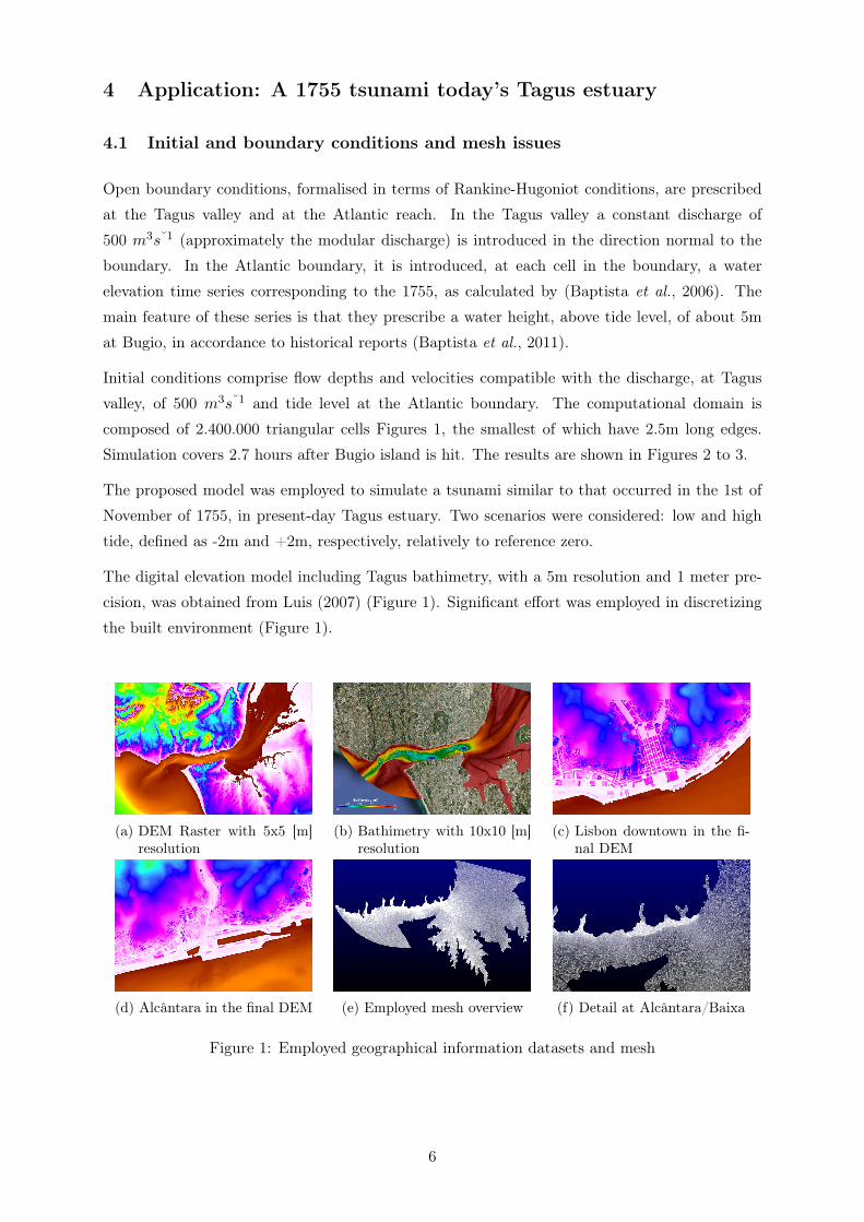
The digital elevation model including Tagus bathimetry, with a 5m resolution and 1 meter pre-

cision, was obtained from Luis (2007) (Figure 1). Significant effort was employed in discretizing

the built environment (Figure 1).

(a) DEM Raster with 5x5 [m]resolution

(b) Bathimetry with 10x10 [m]resolution

(c) Lisbon downtown in the fi-nal DEM

(d) Alcântara in the final DEM (e) Employed mesh overview (f) Detail at Alcântara/Baixa

Figure 1: Employed geographical information datasets and mesh

6

5 Simulation results

5.1 Alcântara

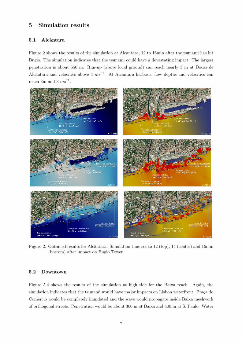
Figure 2 shows the results of the simulation at Alcântara, 12 to 16min after the tsunami has hit

Bugio. The simulation indicates that the tsunami could have a devastating impact. The largest

penetration is about 550 m. Run-up (above local ground) can reach nearly 3 m at Docas de

Alcântara and velocities above 4 ms˘1. At Alcântara harbour, flow depths and velocities can

reach 3m and 3 ms˘1.

Figure 2: Obtained results for Alcântara. Simulation time set to 12 (top), 14 (center) and 16min(bottom) after impact on Bugio Tower

5.2 Downtown

Figure 5.4 shows the results of the simulation at high tide for the Baixa reach. Again, the

simulation indicates that the tsunami would have major impacts on Lisbon waterfront. Praça do

Comércio would be completely inundated and the wave would propagate inside Baixa meshwork

of orthogonal streets. Penetration would be about 300 m at Baixa and 400 m at S. Paulo. Water

7

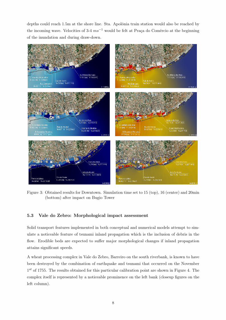
depths could reach 1.5m at the shore line. Sta. Apolónia train station would also be reached by

the incoming wave. Velocities of 3-4 ms−1 would be felt at Praça do Comércio at the beginning

of the inundation and during draw-down.

Figure 3: Obtained results for Downtown. Simulation time set to 15 (top), 16 (center) and 20min(bottom) after impact on Bugio Tower

5.3 Vale do Zebro: Morphological impact assessment

Solid transport features implemented in both conceptual and numerical models attempt to sim-

ulate a noticeable feature of tsunami inland propagation which is the inclusion of debris in the

flow. Erodible beds are expected to suffer major morphological changes if inland propagation

attains significant speeds.

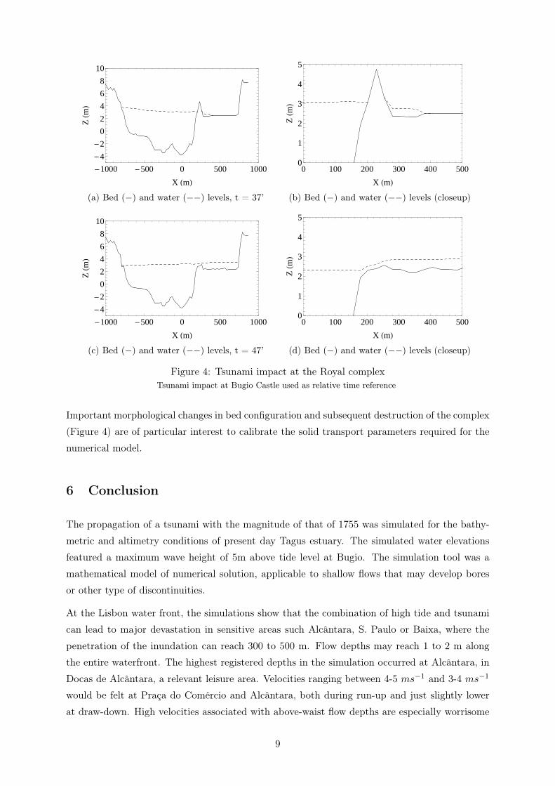
A wheat processing complex in Vale do Zebro, Barreiro on the south riverbank, is known to have

been destroyed by the combination of earthquake and tsunami that occurred on the November

1st of 1755. The results obtained for this particular calibration point are shown in Figure 4. The

complex itself is represented by a noticeable prominence on the left bank (closeup figures on the

left column).

8

-1000 -500 0 500 1000

-4

-2

0

2

4

6

8

10

X m

Zm

(a) Bed (−) and water (−−) levels, t = 37’

0 100 200 300 400 5000

1

2

3

4

5

X m

Zm

(b) Bed (−) and water (−−) levels (closeup)

-1000 -500 0 500 1000

-4

-2

0

2

4

6

8

10

X m

Zm

(c) Bed (−) and water (−−) levels, t = 47’

0 100 200 300 400 5000

1

2

3

4

5

X m

Zm

(d) Bed (−) and water (−−) levels (closeup)

Figure 4: Tsunami impact at the Royal complexTsunami impact at Bugio Castle used as relative time reference

Important morphological changes in bed configuration and subsequent destruction of the complex

(Figure 4) are of particular interest to calibrate the solid transport parameters required for the

numerical model.

6 Conclusion

The propagation of a tsunami with the magnitude of that of 1755 was simulated for the bathy-

metric and altimetry conditions of present day Tagus estuary. The simulated water elevations

featured a maximum wave height of 5m above tide level at Bugio. The simulation tool was a

mathematical model of numerical solution, applicable to shallow flows that may develop bores

or other type of discontinuities.

At the Lisbon water front, the simulations show that the combination of high tide and tsunami

can lead to major devastation in sensitive areas such Alcântara, S. Paulo or Baixa, where the

penetration of the inundation can reach 300 to 500 m. Flow depths may reach 1 to 2 m along

the entire waterfront. The highest registered depths in the simulation occurred at Alcântara, in

Docas de Alcântara, a relevant leisure area. Velocities ranging between 4-5 ms−1 and 3-4 ms−1

would be felt at Praça do Comércio and Alcântara, both during run-up and just slightly lower

at draw-down. High velocities associated with above-waist flow depths are especially worrisome

9

as they are responsible for incorporation of debris and are associated to high casualties.

Important morphological changes are expected in overland tsunami propagation. A known and

fairly well-documented case of morphological impact was used to successfully calibrate the solid

transport features of the numerical model.

The study has shown that some locations of Tagus estuary are vulnerable to tsunami impacts.

Detailed building geometry allowed relevant data to be obtained, which is of particular interest

for designing evacuation plans in case of a major tsunami.

References

Bagnold, R. (1954). Experiments on a gravity-free dispersion of large solid spheres in a newtonian fluidunder shear. In Proceedingsof the Royal Society of London.

Baptista, M.A. & Miranda, J.M. (2009). Revision of the Portuguese catalog of tsunamis. NaturalHazards and Earth System Sciences.

Baptista, M.A., Miranda, J.M. & Luis, J.F. (2006). Tsunami Propagation along Tagus Estuary(Lisbon, Portugal) Preliminary Results. Science of Tsunami Hazards.

Baptista, M.A., Miranda, J.M., Omira, R. & Antunes, C. (2011). Potential inundation of Lisbondowntown by a 1755-like tsunami . Natural Hazards and Earth System Sciences.

Ferreira, R.M.L. (2005). River Morphodynamics and Sediment Transport - Conceptual Model andSolutions. Instituto Superior Técnico.

Ferreira, R.M.L., Franca, M., Leal, J. & Cardoso, A.H. (2009). Mathematical modelling ofshallow flows: Closure models drawn from grain-scale mechanics of sediment transport and flow hydro-dynamics. Canadian Journal of Civil Engineering.

Luis, J.F. (2007). Mirone: A multi-purpose tool for exploring grid data. Computers and Geosciences.

Murillo, J. & García-Navarro, P. (2010). Weak solutions for partial differential equations withsource terms: application to the shallow water equations. Journal of Computational Physics.

Pope, S. (2000). Turbulent Flows. Cambridge University Press.

Roe, P. (1981). Approximate Riemann solvers, parameter vectors and difference schemes. Journal ofComputational Physics.

S.Yalin, M. (1977). Mechanics of Sediment Transport . Pergamon Press.

Synolakis, U.K..C. (1998). Long wave runup on piecewise linear topographies. Journal of Fluid Me-chanics, 374, 1–28.

Toro, E. (2001). Shock-Capturing Methods for Free Surface Shallow Flows. Wiley.

Vázquez-Cedón, M. (1999). Improved treatment of source terms in upwind schemes for the shallowwater equations with irregular geometry . Journal of Computational Physics.

Yeh, H. (1991). Tsunami bore runup. Natural Hazards, 4, 209–220.

10