A Theory of Income Smoothing When

Insiders Know More Than Outsiders∗

Viral Acharya

NYU-Stern, CEPR and NBER

Bart M. Lambrecht

Lancaster University

30 January 2013

Abstract

We develop a theory of income smoothing by firms when insiders know more about

income than outside shareholders, but property rights ensure that outside shareholders

can enforce a fair payout. Insiders report income consistent with outsiders’ expectations

and underproduce in order not to unduly raise expectations about future income. The

observed income and payout process are smooth and adjust partially and over time to-

wards a target. The underproduction problem is more severe the smaller is the inside

ownership and results in an “outside equity Laffer curve”, but the problem is mitigated

by the quality of independent auditing information and by introducing stock-based com-

pensation.

J.E.L.: G32, G35, M41, M42, O43, D82, D92

Keywords: payout policy, asymmetric information, under-investment, accounting qual-

ity, finance and growth.

∗We are grateful to Yakov Amihud, Phil Brown, Peter Easton, Joan Farre-Mensa, Pingyang Gao (dis-

cussant), Oliver Hart, John O’Hanlon, Dalida Kadyrzhanova (discussant), Christian Leuz, Stew Myers,

Lalitha Naveen, Ken Peasnell, Joshua Ronen, Stephen Ryan, Haresh Sapra, Lakshmanan Shivakumar, Pe-

ter Sorensen (discussant) and Steve Young for insightful discussions. We also thank participants at the annual

Real Options conference, the AAA, EFA, RES and NBER summer institute meetings and seminar partic-

ipants at the Universities of Cambridge, Chicago Booth, Lancaster, Nottingham, NYU Stern, Rutgers and

Texas at Austin. Comments can be sent to Viral Acharya (vacharya@stern.nyu.edu) or Bart Lambrecht

(b.lambrecht@lancaster.ac.uk).

A Theory of Income Smoothing When Insiders Know More Than Outsiders

Abstract

We develop a theory of income smoothing by firms when insiders know more about income

than outside shareholders, but property rights ensure that outside shareholders can enforce

a fair payout. Insiders report income consistent with outsiders’ expectations and underpro-

duce in order not to unduly raise expectations about future income. The observed income

and payout process are smooth and adjust partially and over time towards a target. The

underproduction problem is more severe the smaller is the inside ownership and results in

an “outside equity Laffer curve”, but the problem is mitigated by the quality of independent

auditing information and by introducing stock-based compensation.

J.E.L.: G32, G35, M41, M42, O43, D82, D92

Keywords: payout policy, asymmetric information, under-investment, accounting quality, fi-

nance and growth.

1

Introduction

In this paper, we consider a setting in which insiders of a firm have information about income

that outside shareholders do not, but property rights ensure that outside shareholders can

enforce a fair payout based on available information. Under this setting, which is aimed

to capture parsimoniously the relation between a firm’s insiders and outsiders, we ask the

following questions: How is income of the firm reported? How is payout policy of the firm

determined? Is there an effect from asymmetric information on insiders’ production decision,

and how does inside ownership, quality of independent auditing and stock-based compensation

affect this decision? Our model provides theoretical answers to these questions, which lie at

the heart of firm and capital market interactions.

In a seminal paper concerning the firm and capital market interaction, Stein (1989) con-

siders an environment where insiders can pump up current earnings by secretly borrowing at

the expense of next period’s earnings. When the implicit borrowing rate is unfavorable, such

earnings manipulation is value destroying. Stein (1989) shows that insiders do not engage in

manipulation if they only care about current and future earnings. Incentives to manipulate

arise, however, if insiders also care about the firm’s stock price. Since current earnings are

linked to future earnings, pumping up current earnings raises outsiders’ expectations about

future earnings, which in turn feed into the stock price. The market anticipates, however, that

insiders engage in this form of “signal jamming” and is not fooled. Despite the fact that stock

prices instantaneously reveal all information, insiders are “trapped” into behaving myopically.

Thus, stock market pressures can have a dark side, even if markets are fully efficient.

Our paper’s central insight is that myopic behavior by insiders can arise even if the stock

price does not explicitly enter into managers’ objective function. It is sufficient that similar

“market pressures” apply with respect to earnings. We show therefore that myopic managerial

behavior need not necessarily be attributed to stock price considerations. More importantly,

we show that if outsiders cannot directly observe earnings and insiders face capital market

2

pressures then the Stein (1989) result can in fact get reversed in that insiders have an incentive

to manage downwards outsiders’ beliefs about earnings. Unlike Stein (1989) we introduce the

friction that insiders know more than outsiders regarding the firm’s marginal costs and that

insiders face a capital market constraint. We then examine how this affects insiders’ incentives

to engage in myopic behavior.

Asymmetric information leads to potential discrepancies between actual income and out-

siders’ income estimate. This creates incentives for expropriation as insiders may try to fool

outsiders, especially if outsiders’ ownership share is high.1 If outsiders cannot observe net

income directly, but have to infer it indirectly from a noisy output measure (such as sales)

then insiders try to “manage” downwards outsiders’ expectations of current and future in-

come by underproducing and by making production less sensitive to economic shocks. Thus,

in our asymmetric information setting, reported income and payout are smoothed even when

insiders are not directly concerned about the stock price.2 Insiders do so because the capital

market constraint implies that if they inflate earnings they increase outsiders’ current as well

as future payout demands.

Formally, the model works as follows. For the firm to be able to attract outside equity-

holders in the first place, we need investor protection and a credible mechanism that makes

insiders disgorge cash to outside investors. To this end, we call upon the investor protection

framework described in Fluck (1998, 1999), Myers (2000), Jin and Myers (2006), Lambrecht

and Myers (2007, 2008, 2012), Acharya, Myers and Rajan (2011), among others. With the

exception of Jin and Myers (2006) these papers assume symmetric information between in-

siders and outsiders. While under symmetric information outsiders know exactly what they

are due, under asymmetric information outsiders refrain from intervention for as long as the

1If outsiders and insiders own, say, 90% and 10% of the firm, respectively, then under symmetric information

they get 90 and 10, respectively, if actual income is 100 (assuming property rights are strictly enforced). If,

under asymmetric information, insiders could make outsiders believe income is, say, only 90 rather than 100,

then insiders would get 19 instead of 10.2Importantly, since both insiders and outsiders are risk neutral, smoothing does not result from risk aversion.

3

reported income (and corresponding payout) meets their expectations. Therefore, in Jin and

Myers (2006) insiders pay out according to outsiders’ expectations of cashflows and absorb

the residual variation, as is also the case in our model.

We assume that while shocks to marginal costs (modeled by an AR(1) process) are persis-

tent, there is a value-irrelevant “noise” due to measurement error in the output level observed

by outsiders. This noise is transitory, normally distributed, and i.i.d. over time. When observ-

ing an increase in sales (i.e. the noisy proxy of output) outsiders cannot distinguish whether

the increase is due to a reduction in marginal costs (and therefore represents a real increase in

income), or whether the increase is due to value-irrelevant measurement error. Outsiders try

to disentangle the two influences by solving a Kalman filtering problem. Unlike Stein (1989)

(where inference by outsiders is instantaneous and perfect) and Jin and Myers (2006) (where

there is no learning) in our setting outsiders learn gradually over time. Since measurement

errors are transitory and shocks to costs persistent, the underlying source of change becomes

clear only as time passes by. Therefore, outsiders calculate their best estimate of income on

the basis of not only current sales but also past sales. Indeed, while the current sales figure

could be unduly influenced by measurement error, an estimate based on the full sales history

smooths out the effect of these errors.3

Then, in a rational expectations equilibrium outsiders calculate their expectation of actual

income on the basis of the complete history of sales and of what they believe insiders’ optimal

output policy to be. Conversely, insiders determine each period their optimal output policy

given outsiders’ beliefs. We obtain a fixed point (a signal-jamming equilibrium) in which

insiders’ actions are consistent with outsiders’ beliefs and outsiders’ expectations are unbiased

conditional on the information available. Each period outsiders receive a payout that equals

3Formally, outsiders’ income estimate is the solution to a filtering problem. We adopt the Kalman filter

because for our linear model with Gaussian disturbances the Kalman filter is optimal among all possible

estimators and gives an unbiased, minimum variance and consistent estimate of actual (i.e., realized) income.

For an early forecasting application of the Kalman filter in the context of earnings numbers, see Lieber,

Melnick, and Ronen (1983), who use the filter to deal with transitory noise in earnings.

4

their share of what they expect income to be. Insiders also get a payout but they have to

soak up any under (over) payment to outsiders as some kind of discretionary remuneration

(charge): if actual income is higher (lower) than outsiders’ estimate then insiders cash in

(make up for) the difference in outsiders’ payout.

Consequently, reported income and payout are smooth compared to actual income not

because insiders want to smooth income, but because insiders have to meet outsiders’ ex-

pectations to avoid intervention. Two types of income smoothing take place simultaneously:

“financial” smoothing and “real” smoothing. The former is value-neutral and merely alters

the time pattern of reported income without changing the firm’s underlying cash-flows as

determined by insiders’ production decision.4 Insiders also engage in real smoothing by ma-

nipulating production in an attempt to manage outsiders’ expectations. In particular, insiders

under-invest and make output less sensitive to changes in the latent variable affecting marginal

costs. This type of smoothing is value destroying.5 6

Importantly, smoothing has an inter-temporal dimension. The first-best output level is

determined in our model by considerations regarding the contemporaneous level only of the

latent marginal cost variable. But, the current output decision not only affects current sales

levels but also outsiders’ expectations of current and all future income. This exacerbates

the previously discussed underinvestment problem for insiders because bumping up sales now

means the outsiders will expect higher income and payout not only now but also in future.

4For example, DeFond and Park (1997) show that managers increase (decrease) current period discretionary

accruals when current earnings are low (high) and in doing so are borrowing (saving) earnings from (for) the

future. For an illustrative case example of financial smoothing, we refer to the highly publicized settlement

that Microsoft reached with the SEC in 2002. The settlement marked the end to years of investigation by

the SEC over allegations that Microsoft was employing “cookie jar” accounting practices in which it put aside

income in certain quarters to pad future financial results when the company did not meet expectations. Under

the settlement agreement Microsoft is admitting no explicit wrongdoing and is not obliged to pay a fine.5For empirical evidence regarding real smoothing, we refer to section 4.2.6We do not model how real and financial smoothing are implemented in practice. In Ronen and Sadan

(1981), various smoothing mechanisms are discussed and illustrated in great detail.

5

Even though the spillover effect of a one-off increase in sales on outsiders’ future expectations

wears off over time, it still causes insiders to underproduce even more.

Smoothing increases with the degree of information asymmetry between insiders and in-

vestors. Holding constant the degree of information asymmetry (as determined by the variance

of the measurement error), smoothing and underproduction in particular also increase with

outside shareholders’ ownership stake because it increases insiders’ incentives to manage out-

siders’ expectations. Conversely, a higher level of inside ownership leads to less real smoothing.

Indeed, the under-investment problem disappears as insiders move towards 100% ownership.

We show that these effects lead to an “outside equity Laffer curve”: the value of the total

outside equity is an inverted U-shaped function of outsiders’ ownership stake.7

This result suggests that low inside ownership could have detrimental consequences for the

firm. If outside equity is crucial for the development and expansion of owner-managed firms

given their financing constraints, then our results offer a rationale for imposing disclosure

requirements on publicly listed companies and for improving their accounting and auditing

quality. We show that, all else equal, introducing independent accounting information, such as

an unbiased but imprecise income estimate, improves economic efficiency, increases the outside

equity value, and acts as a substitute for a higher inside ownership stake. The implication

is that accounting quality, investments, size of public stock markets, and economic growth

are all positively correlated in our model, as found in the empirical literature on finance and

growth (King and Levine (1993), Rajan and Zingales (1998)).

In a final extension, we embed in Section 3.4 the effect of stock-based compensation for

insiders as in the Stein (1989) model. We show that this dampens but does not eliminate

insiders’ incentives to engage in under-production in our model: there is now a tradeoff that

insiders face between raising stock price (which benefits them through stock-based compensa-

7The analogy with the taxation literature is straightforward: outsiders’ ownership stake acts ex post like

a proportional tax on distributable income and undermines insiders’ incentives to produce. Note that our

under-investment result does not require the presence of costly effort by insiders.

6

tion) and paying out higher dividends in future (since higher stock prices arise due to greater

outsider expectations).

The paper is organized as follows. Section 1 presents the benchmark case with symmetric

information between outsiders and insiders. Section 2 analyzes the asymmetric information

model. Section 3 discusses the robustness and extensions of the model, in particular, the

insiders’ participation constraint, the value of audited disclosure, and the effect of stock-based

insider compensation. Section 4 presents novel empirical implications that flow from our model

for (1) the time-series and cross-sectional properties of corporate income, (2) real smoothing

by firms, (3) corporate ownership structure, and (4) public versus private firms. Section 5

relates our paper to existing literature. Section 6 concludes. Proofs are in the appendix.

1 Symmetric information case

Consider a firm with access to a productive technology. The output from the technology is

sold at a fixed unit price, but its scale can be varied. Marginal costs of production follow

an AR(1) process and are revealed each period before the output scale is chosen. A part of

the firm is owned by risk-neutral shareholders (outsiders) and the rest by risk-neutral insiders

who also act as the technology operators. To start with, we focus on the first-best scenario in

which there is congruence of objectives between outsiders and insiders, and information about

marginal costs is known symmetrically to both outsiders and insiders.

Formally, we consider a firm with the following income function:

πt = qt −q2t

2xt(1)

where xt = Axt−1 + B + wt−1 with wt−1 ∼ N(0, Q) , (2)

where qt denotes the chosen output level. The (inverse) marginal production cost variable

xt follows an AR(1) process with auto-regressive coefficient A ∈ [0, 1), a drift B, and an

7

i.i.d. noise term wt−1 with zero mean and variance Q.8 The output level qt is implemented

after the realization of wt−1 is observed.

All shareholders are risk-neutral, can borrow and save at the risk-free rate, and have a

discount factor β ∈ (0, 1). Therefore -unlike Stein (1989)- changing the time pattern of cash

flows (without changing their present value) through more borrowing or saving is costless.

The value of the firm is given by the present value of discounted income:

Vt = maxqt+j ,j=0...∞

Et[∞∑j=0

βjπt+j] = maxqt+j ,j=0...∞

Et

[∞∑j=0

βj(qt+j −

q2t+j

2xt+j

)](3)

Then, the first-best production policy that maximizes firm value is as follows.

Proposition 1 The first-best production policy is qot = xt . The firm’s realized income and

total payout under the first-best policy are given by: πot = xt2.

The first-best output level qot equals xt. Recall that a higher value for xt implies lower

marginal costs. Therefore, the output level rises with xt. As xt goes to zero, marginal costs

spiral out of control and the first-best output quantity goes to zero.9

8Our model generalizes to the case where xt follows a random walk with drift (i.e. A = 1). Mean reversion

(i.e. A < 1) is, however, a more realistic assumption for production costs. For example, commodity prices

(which constitute a large component of production costs in some industries) are often mean reverting due to

the negative relation between interest rates and prices.9 Since the shocks that drive xt are normally distributed, marginal costs could theoretically become negative.

The solution in proposition 1 no longer makes sense for negative xt because marginal costs can, of course,

not be negative. The likelihood of negative values for xt arising is, however, negligibly small if the stationary

unconditional mean of xt (given by B1−A ) is sufficiently large relative to the unconditional variance of xt (given

by Q1−A2 ). We assume this condition to be satisfied so that we can safely ignore the occurrence of negative

costs. To rule out negative values for xt altogether one could assume that xt is log-normally distributed. This

would, however, make the Bayesian updating process deployed in next section completely intractable. The

normality assumption is standard in the information economics literature (for example, Grossman (1976) and

papers that originated from this seminal paper).

8

1.1 Inside and outside shareholders

We now introduce inside and outside shareholders who, respectively, own a fraction (1 − ϕ)

and ϕ of the shares, ϕ ∈ [0, 1]. For example, insiders (managers and even board members

involved in the firm’s operating decisions) typically own the majority of shares of private

firms (ϕ < 0.5), whereas for public firms it is more common that outsiders own the majority

of shares (ϕ > 0.5). Insiders set the production (qt) and payout (dt) policies. Analogous to

Myers (2000), Jin and Myers (2006), Lambrecht and Myers (2007, 2008, 2012), and Acharya,

Myers and Rajan (2011), we assume that insiders operate subject to a threat of collective

action. Outsiders’ payoff from collective action is given by ϕαVt where α (∈ (0, 1]) reflects the

degree of investor protection (or specificity of the firm’s technology).10

To avoid collective action, insiders pay out each period a dividend dt that leaves outsiders

indifferent between intervening and leaving insiders unchallenged for another period. If St

denotes the value of the outside equity then dt is defined by:11

St = dt + βαϕEt[Vt+1] = αϕVt (4)

⇐⇒ dt + βαϕEt[Vt+1] = αϕπt + αϕβEt[Vt+1] ⇐⇒ dt = αϕπt (5)

Equation (4) can be interpreted as a capital market constraint that requires insiders to provide

10When we have a public corporation with a large outside ownership stake, then collective action is as

described in the Myers (2000) “corporation model”. Outsiders take over the firm and displace insiders. The

cost of collective action reflects the loss in managerial human capital, deadweight costs of getting organized,

etc. If we have a private company with a small outside ownership stake then outsiders are minority stakeholders

and the inside majority rules. Minority shareholders are, however, not entirely impotent as company law or

commercial code grants minority shareholders either a judicial venue to challenge the decisions of management

or the right to step out of the company by requiring the company to purchase their shares. The payoff from

collective action to outside minority shareholders under this “oppressed minorities mechanism” (see La Porta

et al. (1998)) is therefore the fair value of their stake, net of any costs of intervention (such as a possible

minority discount or legal costs).11It is not strictly necessary that all income is paid out each period. If reported income earns the risk-free

rate of return within the firm (e.g. through a high yield cash account) and is protected from expropriation by

insiders, then outsiders do not require income to be paid out (see Lambrecht and Myers, 2012).

9

an adequate return to outside investors.12

ϕ denotes outsiders’ “nominal” ownership stake. Scaling the nominal ownership stake

by the degree of investor protection α gives outsiders’ effective or “real” ownership state

θ ≡ ϕα. It follows that the payouts to outsiders (dt) and insiders (rt) are respectively given

by θπt and (1− θ)πt. Income (πt) is shared between insiders and outsiders according to their

real ownership stake. The following corollary results at once.

Corollary 1 With symmetric information, insiders adopt the first-best production policy, and

payout to outsiders (insiders) equals a fraction θ (1− θ) of realized income πt.

2 Asymmetric information

We now add two new ingredients to the model. First, we assume that the actual realizations

of the stochastic marginal cost variable xt are observed by insiders only. All model parameters

remain common knowledge, however. Outsiders also have an unbiased estimate x0 of the initial

value x0.13 Second, outsiders cannot observe the output level qt, but have to rely on some

noisy proxy. This introduces measurement error. Instead of observing qt, outsiders observe

st ≡ qt + εt where εt is an i.i.d. normally distributed noise term with zero mean and variance

R (i.e., εt ∼ N(0, R)). The measurement error is uncorrelated with the marginal cost variable

xt (i.e., E(wkεl) = 0 for all k and l). In what follows we refer to st as the firm’s “sales” as

perceived by outsiders, i.e., outsiders perceive the firm’s revenues to be st, whereas in reality

they are qt. st can, for example, be interpreted as analysts’ estimate of output. We assume

this estimate to be noisy, but unbiased (i.e. E(εt) = 0).

12Graham et al. (2005) provide convincing evidence of how capital market pressures induce managers to

meet earnings targets at all costs. As one surveyed manager put it:“I miss the target, I’m out of a job.”

Mergenthaler et al. (2012) find that CEOs are penalized via bonus cuts, fewer equity grants, and forced

turnover when they just miss the latest consensus analyst forecast.13x0 is revealed to outside investors when the firm is set up at time zero (see section 3.2).

10

Outsiders are aware that sales are an imperfect proxy for economic output and they know

the distribution from which εt is drawn. Importantly, insiders implement output (qt) after the

realization of xt but before the realization of εt is known. Since εt is value-irrelevant noise, the

firm’s actual income is still given by π(qt) = qt − q2t2xt

. However, as qt and xt are unobservable

outsiders have to estimate income on the basis of noisy sales figures. Therefore measurement

errors can lead to misvaluation in the firm’s stock price (unlike Stein (1989) where stock prices

are strong-form efficient).

We know from previous section that there is a mapping from the latent variable xt to

both qt and πt. The presence of the noise term εt obscures, however, this link and makes it

impossible for outsiders exactly to infer xt and πt from sales. Assuming that insiders cannot

trade in the firm’s stock and that the information asymmetry cannot be mitigated through

monitoring or some other mechanism, the best outsiders can do is to calculate a probability

distribution of income, πt, on the basis of all information available to them. This information

set It is given by the full history of current and past sales prices, i.e., It ≡ {st , st−1 , st−2 ...}.

We show that on the basis of the initial estimate x0 and the sales history, It, outsiders can

infer a probability distribution for the latent marginal cost variable xt, which in turn maps

into a probability distribution for income πt. Outsiders then use this distribution to calculate

their estimate πt of the firm’s income, i.e. πt = E[πt|It] ≡ ES,t(πt), where the subscript S in

ES,t[πt] emphasizes (outside) shareholders’ expectation at time t of πt based on the information

set It.

The capital market constraint requires that dt satisfies the following constraint:

St = dt + βϕαES,t[Vt+1] = ϕαES,t[Vt]

⇐⇒ dt + βϕαES,t[Vt+1] = ϕαES,t[πt] + ϕαβES,t[Vt+1] ⇐⇒ dt = θES,t[πt]

Therefore, to avoid collective action insiders set the payout equal to dt = θES,t(πt). In other

words, outsiders want their share of the income they believe has been realized according to all

information available to them. While insiders cannot manage outsiders’ expectations through

words (which are not credible) they can do so through their actions. Managers can influence

11

observable sales (st) and therefore πt by their chosen output level (qt).

Insiders’ optimization problem can now be formulated as follows:

Mt = maxqt+j ;j=0..∞

Et

[∞∑j=0

βj (π(qt+j) − θES,t+j [π (qt+j)])

](6)

with insiders’ optimal output policy qt being an equilibrium (fixed point) once outsiders’ beliefs

are fixed. The complete derivation of the solution is given in the appendix. We briefly present

a heuristic derivation of the rational expectations equilibrium here. Outsiders conjecture that

insiders’ production policy is given by qt = Hxt, where H is some constant. Therefore,

ES,t+j [π(qt+j)] =(H − H2

2

)ES,t+j [xt+j] ≡ hES,t+j [xt+j]. Define xt ≡ ES,t[xt] as outsiders’

estimate of the latent variable xt conditional on the information available at time t. Since

st = qt + εt and qt = Hxt, sales are an imperfect (noisy) measure of the latent variable xt,

as is clear from the following “measurement equation”:

st = H xt + εt with εt ∼ N(0, R) (7)

Outsiders also know the variance R of the noise, εt, and the parameters A, B and Q of the

“state equation”:

xt = Axt−1 + B + wt−1 with wt ∼ N(0, Q) for all t (8)

Outsiders now solve what is known as a “filtering” problem. Using the Kalman filter (see

appendix), the measurement equation can be combined with the state equation to make

inferences about xt on the basis of current and past observations of st. This allows outsiders to

form an estimate of actual income πt. While the measurement equation is usually exogenously

given, our Kalman filter has the novel feature that the constant slope coefficient H in the

measurement equation is set endogenously by insiders.

The Kalman estimator xt is unbiased (see Chui and Chen (1991) page 40). The Kalman

filter is optimal (“best”) in the sense that it minimizes the mean square error (Gelb (1974)).

The solution is formulated in terms of the steady state or “limiting” Kalman filter which is the

estimator xt for xt that is obtained after a sufficient number of measurements st have taken

12

place over time for the estimator to reach a steady state.14 The steady-state estimator allows

us to analyze the long-run behavior of reported income and payout and is given by (Chui and

Chen (1991), p78):

xt = (Axt−1 +B)λ + Kst (9)

where λ and K are as defined in the proposition. K is called the “Kalman gain” and it plays

a crucial role in the updating process. Substituting xt−1 in (9) by its estimate, one obtains

after repeated substitution:

xt = Bλ[1 + λA+ λ2A2 + λ3A3 + ...

]+ K

[st + λAst−1 + λ2A2st−2 + λ3A3st−3 + ...

]=

Bλ

1− λA+ K

∞∑j=0

λjAjst−j . (10)

Thus, outsiders’ estimate of current actual income is not only determined by their observation

of current sales but also by the whole history of past sales. Hence, insiders’ optimization

problem is no longer static but inter-temporal and dynamic. Indeed, the current production

decision not only affects insiders’ expectations about current but also future income.

Substituting outsiders’ beliefs ES,t+j[π(qt+j)] = hxt+j into insiders’ objective function,

insiders optimize:

Mt = maxqt+j ;j=0..∞

Et

[∞∑j=0

βj (π(qt+j) − θhxt+j)

](11)

which gives the following first-order condition:

∂Mt

∂qt= 1 − qt

xt− θhK − θhKβλA − θhK (βλA)2 − θhK (βλA)3 − ... = 0 (12)

Or equivalently:

qt =

[1 − θhK

1− βλA

]xt (13)

14If the disturbances (εt and wt) and the initial state (x0) are normally distributed then the Kalman filter

is unbiased. When the normality assumption is dropped unbiasedness may no longer hold, but the Kalman

filter still minimizes the mean square error within the class of all linear estimators. Under mild conditions

(see footnote 29 in the appendix) the Kalman filter converges to its steady state. Convergence is of geometric

order and therefore fast.

13

Outsiders’ conjectured output policy qt = Hxt is a fixed point if and only if:

H = 1 − θhK

1− βλA(14)

At the fixed point, outsiders’ expectations are rational given insiders’ output policy, and in-

siders’ output policy is optimal given outsiders’ expectations. Rearranging (14) gives equation

(19) in proposition 2, which pins down the equilibrium value for H. Note that the right hand

of equation (14) is less than (or equal to) one, and therefore insiders underproduce (i.e. H ≤ 1)

compared to what is first best. The results are summarized in the following proposition.

Proposition 2 The insiders’ optimal production plan is given by:

qt = H xt = Hqot for all t (15)

Payout to outside shareholders equals a fraction θ of reported income: dt = θπt where

πt =

(H − H2

2

)xt ≡ hxt , (16)

and where xt = (Axt−1 + B)λ + K st (17)

=λB

1− λA+ K

∞∑j=0

(λA)jst−j . (18)

H is the positive root to the equation:

f(H) ≡ H2K(θ

2− βA) +H [βA(1 +K)− 1− θK] + 1− βA = 0 (19)

with K ≡ HPH2P+R

, λ ≡ (1−KH) and P is the positive root of the equation:

P = A2P − A2H2P 2

H2P +R+ Q . (20)

The error of outsiders’ income estimate (πt − πt) is normally distributed with mean zero (i.e.,

ES,t[πt − πt] = 0) and variance σ2 ≡ ES,t[(πt − πt)2] = h2 P .

2.1 Production Policy

We know from Proposition 2 that insiders’ optimal production policy is given by qt = H xt

where H is the solution to equation (19). There exists a unique positive (real) root for H

14

which lies in the interval (0, 1].15 We therefore obtain the following corollary.

Corollary 2 If outsiders indirectly infer income from sales (st) then insiders underproduce

(i.e., qt = Hxt = Hqot ≤ q0t ).

Insiders underproduce because outsiders do not observe xt directly but estimate its value

indirectly from sales. This gives insiders an incentive to manipulate sales (engage in “signal-

jamming”) in an attempt to “fool” outsiders. In particular, insiders trade off the benefit from

lowering outsiders’ expectations about income against the cost of underproduction. Insiders’

first-order condition (12) shows that a marginal decrease in current output (and therefore

expected sales) lowers outsiders’ beliefs about current income by hK, and about income j

periods from now by hK(λA)j. Therefore, a marginal cut in output benefits insiders. Insiders

keep cutting output up to the point where the marginal cost of cutting (in terms of realized

income) equals the marginal benefit (in terms of lowering outsiders’ expectations).16

The unconditional long-run mean for qt under the first-best and actual production policies

are, respectively, E[qot ] = E[xt] = B/(1 − A) and E[qt] = HE[xt] = BH/(1 − A). Lost

output, in turn, translates into a loss of income. The unconditional mean income under the

first-best and actual production policies are, respectively, E[πot ] = 12E[xt] and E[πt] = hE[xt].

The following corollary then explains the effect of asymmetric information on the produc-

tion decision.

15f(0) = −1 + βA < 0 and f(1) = θK2 ≥ 0. Therefore, ∃H ∈ (0, 1] for which f(H) = 0. Since θ, A,

λ and β all fall in the [0, 1] interval, an exhaustive numerical grid evaluation can be executed for all possible

parameter combinations. Numerical checks reveal that H is the unique positive root.16Note that outsiders are not fooled by insiders’ signal-jamming. In equilibrium, outsiders correctly antic-

ipate this manipulation and incorporate it into their expectations. Nevertheless, insiders are “trapped” into

behaving myopically. The situation is analogous to what happens in a prisoner’s dilemma. The preferred

cooperative equilibrium would be efficient production by insiders and no conjecture of manipulation by out-

siders. This can, however, not be sustained as a Nash equilibrium (as in Stein (1989)) because insiders have

an incentive to underproduce whenever outsiders believe the efficient production policy is being adopted.

15

Corollary 3 The noisier the link between the latent variable (xt) and its observable proxy

(st), the weaker insiders’ incentive to manipulate the proxy by underproducing. In particular,

insiders’ production decision converges to the first-best one as the variance of measurement

errors becomes infinitely large (R → ∞) or as uncertainty with respect to the latent variable

xt decreases (Q → 0), i.e., limQ→0H = limR→∞H = 1. Conversely, the more precise the

link between st and xt, the higher the incentive to underproduce. The lower bound for H is

achieved for the limiting cases Q→∞ and R→ 0, i.e., limQ→∞H = limR→0H = 1− θ2−θ .

When xt becomes deterministic (Q = 0) then the estimation error with respect to xt, goes to

zero (i.e., P → 0). This means that the Kalman gain coefficient K becomes zero too (there is

no learning). But if there is no learning (K = 0 and λ = 1) then insiders’ output decision qt

no longer affects outsiders’ estimate of the cost variable, as illustrated by equation (9). As a

result the production policy becomes efficient (i.e., H = 1 and qt = xt).

Similarly, if there are measurement errors then the link between sales and the latent cost

variable becomes noisy. This mitigates the under-investment problem, because the noise

obscures insiders’ actions and therefore their incentive to cut production.

In the absence of measurement errors (R = 0) the link between sales st and the contempo-

raneous level of the latent variable xt becomes deterministic.17 Outsiders know for sure that an

increase in sales results from a fall in marginal costs. Therefore, when observing higher sales,

outsiders want higher payout. In an attempt to manage outsiders’ expectations downwards,

insiders underproduce. If R = 0 then we get the efficient outcome (H = 1) only if insiders

get all the income (θ = 0); otherwise we get under-investment (H < 1). As the insiders’ stake

of income goes to zero (θ → 1) also production goes to zero (i.e., H → 0). Both outsiders

and insiders get nothing, even though the firm could be highly profitable! This result is in

sharp contrast with the symmetric information case where the efficient outcome is obtained

no matter how small the insiders’ share of the income. Thus, for firms where insiders have

17For R = 0 we get P = Q, K = 1/H and λ = 0. Therefore, from Proposition 2 it follows that xt = st/H

and st = Hxt. Consequently, xt = xt.

16

a very small ownership stake (e.g. public firms with a highly dispersed ownership structure),

asymmetric information and the resulting indirect inference-making process by outsiders could

undermine the firm’s very existence, an issue we return to in section 3.

Figure 1 illustrates the effect of the key model parameters (R,Q,A and θ) on production

efficiency. Efficiency is measured with respect to two different variables: the unconditional

mean output (E[qt]), and unconditional mean income (E[πt]). The degree of efficiency is

determined by comparing the actual outcome with the first-best outcome, i.e., E[qt]/E[qot ] =

H (dashed line), and E[πt]/E[πot ] = 2h (solid line).

The figure shows that the efficiency loss is larger with respect to output than income

because the loss in revenues due to underproduction is to some extent offset by lower costs

of production. Panel A and B confirm that full efficiency is achieved as R moves towards ∞

and for Q = 0. Panel C shows that a higher autocorrelation in marginal costs substantially

reduces efficiency because it allows outsiders to infer more information about the latent cost

variable from sales and therefore gives insiders stronger incentives to distort production.

Finally, panel D shows that production is fully efficient if outsiders have no real stake in

the firm’s income (i.e., θ = 0). Efficiency severely declines as outsiders’ stake increases. For

θ = 1, insiders achieve only 28% of the first-best output level. However, one can show that

as Q/R → 0 incentives are fully restored, and the first-best outcome can be achieved even

for θ = 1. This confirms that the root cause of underproduction is the process of indirect

inference and not the outside ownership stake per se. The firm’s ownership structure serves,

however, as a transmission mechanism through which inefficiencies can be amplified.

2.2 The time-series properties of income

Proposition 2 also allows us to derive the time-series properties of income:

Proposition 3 The firm’s “actual income” is πt = hxt. The firm’s “reported income”, πt(=

17

ES,t[πt] = hxt), is described by the following target adjustment model:

πt = πt−1 + (1− λA) (π∗t − πt−1) (21)

= λAπt−1 + Khst + hλB ≡ γ2πt−1 + γ1 st + γ0 . (22)

The “income target” π∗t is given by:

π∗t =hλB

1− λA+

(Kh

1− λA

)st ≡ γ∗0 + γ∗1 st . (23)

The speed of adjustment coefficient is given by SOA ≡ (1− λA) with 0 < SOA ≤ 1.

The proposition characterizes three types of income: the “income target” (π∗t ), “reported

income” (πt) and “actual income” (πt). Reported income follows a target that is determined

by the contemporaneous level of sales. However, as equation (21) shows, the reported income

only gradually adjusts to changes in sales because the SOA coefficient (1− λA) is less than

unity. This leads to income smoothing in the sense that the effect on reported income of a shock

to sales is distributed over time. In particular, a dollar increase in sales leads to an immediate

increase in reported income of only hK. The lagged incremental effects in subsequent periods

are given by hKλA, hK(λA)2, hK(λA)3,... The long-run effect of a dollar increase in sales

on reported income equals hK∑∞

j=0 (λA)j = hK1−λA , which is the slope coefficient γ∗1 of the

income target π∗t (see equation (23)). In contrast, with symmetric information, the impact of

a shock to sales is fully impounded into reported income immediately.

Intuitively, reported income only partially adjusts to a contemporaneous shock in sales

because in the short run outsiders cannot distinguish between a transitory measurement error

and a persistent shock to the latent cost variable. However, as subsequent sales are observed

the transitory or persistent nature of the shock is gradually revealed. Reported income can

therefore also be expressed as a distributed lag model in which it is a function of current and

past sales, by repeated backward substitution of equation (22):

πt =hλB

1− λA+ Kh

∞∑j=0

(λA)j st−j . (24)

The following corollary then summarizes how asymmetric information affects income:

18

Corollary 4 Measurement errors create asymmetric information, which in turn leads to

smoothing of reported income. A lower degree of information asymmetry (i.e., R falls rel-

ative to Q) leads to less smoothing. In the limit (i.e., R = 0 or Q→∞) both reported income

and target income coincide with actual income at all times (i.e., πt = πt = π∗t for all t).

No financial smoothing whatsoever occurs when R = 0 because in that case all information

asymmetry is eliminated. In the absence of measurement errors, it is possible to infer the

marginal cost variable xt with 100% accuracy from the observed sales figure st. The same

result obtains when Q → ∞ because in that case measurement errors are negligibly small

compared to the variance of the latent cost variable. This important result confirms again

that asymmetric information and not uncertainty per se is the root cause of income smoothing.

The corollary also confirms that as the degree of information asymmetry goes to zero, our

rational expectations equilibrium converges to the simple sharing rule that prevails under

symmetric information. Indeed: limR→0 dt = θ limR→0 πt = θπt. Finally, given that (i)

reported income is smooth relative to actual income and (ii) payout is based on reported

income, it follows that insiders soak up the variation. We address this issue next in Section

2.3, where we discuss payout.

2.3 Payout Policy

Since the payout to outsiders is given by dt = θπt, it follows that the firm’s payout policy to

outsiders is described by the target adjustment model for πt in (22):

dt = λAdt−1 + θhKst + θhλB . (25)

The payout model is similar to the well known Lintner (1956) dividend model. The key

difference is that in Lintner (1956) the payout target is determined by the firm’s net income,

whereas in our model the target is a function of sales because net income is not directly

observed by outsiders. Payout in our model is not smoothed relative to reported income but

19

relative to a proxy variable observable by outsiders, i.e., sales.18

3 Robustness, extensions and discussion

3.1 Independent audited disclosure and ownership structure

Our analysis in section 2 showed that the firm’s production policy becomes increasingly more

inefficient as insiders’ real ownership stake (1− ϕα) decreases. This could pose serious prob-

lems for public firms, which often have a small inside equity base. Our model predicts that

under-investment could become so severe that firms stop producing altogether, even if they

are inherently profitable. It may therefore come as no surprise that mechanisms have been

developed to reduce the degree of information asymmetry. In particular, publicly traded com-

panies (unlike private firms) are subject to stringent disclosure requirements. The traditional

argument put forward to justify disclosure is often that of investor protection. The general

underlying idea is that outside investors need to be protected from fraud or conflicts of in-

terests by insiders (usually managers). Audited disclosure is generally believed to benefit

outsiders by curtailing insiders’ ability to exploit their informational advantage and to extract

informational rents.

Our paper shows that the case for audited accounting information rests not only on investor

protection. Our model shows that asymmetric information is problematic even if insider trad-

ing is precluded and outsiders’ property rights are 100% guaranteed (i.e., α = 1). Moreover,

disclosure is not necessarily a win/lose situation for outsiders/insiders. In our setting, elim-

inating information asymmetry would be welcomed by outsiders and insiders alike. In other

words, disclosure (assuming it can be achieved in a relatively costless fashion) is a win-win

18Payout smoothing in the strict Lintner sense obtains, e.g., if insiders are risk-averse and subject to habit

formation. Lambrecht and Myers (2012) show that insiders of this type smooth payout relative to income by

borrowing and lending.

20

situation for all parties involved.

Formally, in proposition 2 we showed that, on the basis of current and past sales, outsiders

calculate an income estimate πt. The error of outsiders’ estimate, πt − πt, is normally dis-

tributed with zero mean and variance σ2. Suppose now that, in addition to the sales data,

auditors provide each period an independent estimate yt of income where yt ∼ N(πt, σ2).

Importantly, auditors provide their assessment after εt and wt−1 are realized. The auditors’

estimate is unbiased (i.e., Et[yt] = πt) but subject to some random error (yt − πt). Insid-

ers nor auditors have control over the error, and the error is independent across periods. In

summary, on the basis of the full sales history It outsiders construct a prior distribution of

current income that is given by N(πt, σ2). Auditors then provide an independent estimate yt,

which outsiders know is drawn from a distribution N(πt, σ2). As will become clear, auditor

independence (i.e. insiders cannot influence auditors’ perception of income) is key.

Using simple Bayesian updating, it follows that the outsiders’ estimate of income condi-

tional on yt and on the sales history It is given by:19

κyt + (1− κ)πt where κ =σ2

σ2 + σ2. (26)

The parameter κ can be interpreted as a parameter that reflects the quality of the additional

information provided. A value of κ close to 0 means that the audited disclosure is highly

unreliable and carries little weight in influencing outsiders’ beliefs about income.

How does the provision of information by independent auditors influence insiders’ deci-

19It might be possible for outsiders to refine the estimate of the latent cost variable xt by using the entire

history of auditors’ income estimates. We ignore this possibility, and assume that all relevant accounting

information is encapsulated in the auditors’ most recent income estimate.

21

sions? Insiders’ optimization problem can now be formulated as:

Mt = maxqt+j ;j=0..∞

Et

[∞∑j=0

βj (π(qt+j) − ϕακEt+j(yt+j) − ϕα(1− κ)ES,t+j [π (qt+j)])

]

= maxqt+j ;j=0..∞

Et

[∞∑j=0

βj (π(qt+j) (1− ϕακ) − ϕα(1− κ)ES,t+j [π (qt+j)])

]

= (1− ϕακ) maxqt+j ;j=0..∞

Et

[∞∑j=0

βj (π(qt+j) − G(ϕ, α, θ)ES,t+j [π (qt+j)])

](27)

where G(ϕ, α, κ) ≡ ϕα(1−κ)1−ϕακ ≡

θ(1−κ)1−θκ , and where we made use of the fact that the auditors’

estimate is unbiased at all times, i.e., Et+j[yt+j] = π(qt+j) for all j, irrespective of insiders’

decision rule for qt+j. In other words, insiders cannot distort auditors’ estimate (the release

of the accounting information by independent auditors occurs after income is realized).

Comparing the optimization problem (27) with the original one we solved in (6), one can

see that both problems are essentially the same, except for the fact that the outside ownership

parameter θ in (6) has been replaced by the governance index G(ϕ, α, κ) in (27). This means

that the solution for qt+j can be obtained by merely replacing θ by G(ϕ, α, κ) in the solution

we previously obtained.

G(ϕ, α, κ) ranges across the [0, 1] interval and can be interpreted as an (inverse) governance

index that crucially depends on the outsiders’ ownership stake (ϕ), the degree of investor

protection (α) and on the quality of audited disclosure (κ). If κ = 0 (i.e., G = θ) then

the independently provided accounting information is completely unreliable and discarded

by outsiders. In that case the optimization problem and its solution coincide exactly with

the ones presented in section 2. If κ = 1 (i.e., G = 0) then the independently provided

accounting information is perfectly reliable. All information asymmetry is resolved and we

get the first-best outcome that was presented in section 1. Since ∂G(θ,κ)∂κ

≤ 0, it follows that:

Corollary 5 Higher quality audited disclosure (κ) improves the firm’s operating efficiency.

22

3.2 Accounting quality, stock market size and growth

In this section we examine the model’s implications for corporate investment (and economic

growth more generally) by analyzing the initial decision to set up the firm.

Assume that an investment cost E is required to establish the firm at time t = 0. The

financing is raised from inside and outside equity. To abstract from adverse selection issues

(see Myers and Majluf (1984)) we assume that insiders have access to an unbiased estimate

for x0 at time zero (i.e., x0 = x0). As a result insiders and outsiders attach the same value

V (x0; θ, κ) to the firm when the firm is founded, as given in the following proposition.

Proposition 4 The value of the firm at time t = 0 is given by:

V0(x0; θ, κ) =h

(1− βA)

(x0 +

Bβ

1− β

)(28)

where the determinant h of the production policy (h ≡ H − H2

2) is obtained as described in

proposition 2 but by replacing θ by G(θ;κ) in equation (19).

We know that the firm value monotonically declines in the real ownership stake θ(≡ αϕ) and

that the first-best firm value is achieved when the outside ownership stake is zero (i.e., θ = 0).

Assuming the investment in the firm happens on a now-or-never basis at t = 0, the first-best

investment decision is given by the following criterion: invest if and only if V (x0; θ = 0, κ) ≥ E.

Note that the accounting quality κ does not influence the investment decision when θ = 0,

because without outside investors audited disclosure becomes superfluous.

Assume next, without loss of generality, that insiders have no money to contribute and

need to raise the full amount E from outsiders. Assume further that the quality of audited

disclosure (κ) is exogenously given, but that the real ownership stake θ can be chosen. The

decision problem is therefore to identify the lowest value for θ that allows insiders to raise

enough outside equity, St, to cover the investment cost (i.e., S0(x0; θ, κ) = E).

23

Since x0 = x0, the initial inside (M0) and outside (S0) equity values are:

M0 = V0(x0; θ, κ)− θES,0 [V0(x0; θ, κ)] = (1− θ)V0(x0; θ, κ) (29)

S0 = θES,0 [V0(x0; θ, κ)] = θV0(x0; θ, κ) (30)

The (constrained) optimal value for θ is therefore the solution to:

θo = min {θ| θV0(x0; θ, κ) = E} (31)

The solution is illustrated in Figure 2. Panel A plots the total firm value V0(x0; θ, κ) as a

function of outsiders’ real ownership θ for three different levels of disclosure quality (κ). In

line with our earlier results, total firm value declines monotonically with respect to θ. The

loss can be substantial: the first-best firm value equals 1900 (i.e., for θ = 0), whereas the

firm value under 100% outside ownership equals a mere 920 (i.e., for θ = 1). High quality

audited disclosure (κ = 0.9) can, however, significantly mitigate the value loss. For example

for κ = 0.9 the loss in value appears to be less than 1% for as long as insiders own a majority

stake. In the absence of audited disclosure or when audited disclosure is completely useless

(i.e., κ = 0), significant value losses kick in at much lower outside ownership levels. For

example, at θ = 0.5 about 10% of the first-best value is lost.

Panel B shows the total outside equity value as a function of the outside ownership stake

for three different levels of disclosure quality. The curves resemble “outside equity Laffer

curves”.20 The outside equity value θV0(x0; θ, κ) is an inverted U-shaped function of θ that

reaches a unique maximum. This maximum changes significantly according to the quality of

the audited disclosure, and equals about 1550, 1200 and 1020 for high quality, low quality and

no audited disclosure, respectively. No investment would take place in the absence of audited

disclosure, because the amount of outside equity that can be raised is inadequate to finance

the investment cost (which equals E = 1100). Investment would take place in the two cases

20The traditional Laffer curve is a graphical representation of the relation between government revenue

raised by taxation and all possible rates of taxation. The curve resembles an inverted U-shaped function that

reaches a maximum at an interior rate of taxation.

24

where accounting information is audited, and about θo = 58% (θo′

= 63%) of shares would

end up in outsiders’ hands with high (low) quality audited disclosure.

Our results provide theoretical support for a number of empirical studies that have found

a positive link between economic growth, stock market size, stock market capitalizations, and

quality of accounting information. The standard explanation for this result is that higher

quality accounting information provides better investor protection. While higher investor

protection (i.e., higher α) also leads to higher stock market valuations in our model, audited

disclosure does not as such improve investor protection in our model. Instead, independent

audited disclosure reduces the inefficiencies from indirect inference because insiders are less

concerned about the effect of their actions on outsiders’ expectations. Our model therefore

highlights an important role of independent audited disclosure and monitoring that has hith-

erto not been recognized in the literature.

3.3 Forced disclosure and the “big bath”

Insiders’ payout policy guarantees that the capital market constraint is satisfied at all times,

i.e., St ≥ ϕαEt[Vt|It]. But will insiders be willing to adhere to this payout policy under all

circumstances? Insiders’ participation constraint is satisfied if they are better off paying out

than triggering collective action. Collective action implies that stockholders “open up” the

firm and uncover its true value (Vt). It is reasonable (although not necessary) to assume that

collective action also imposes a cost upon insiders. Without loss of generality assume that

these costs are proportional to the firm value and given by Ct = cVt.

“Forced disclosure” pricks the bubble that has been building up over time and brings

outsiders’ beliefs about the firm value back to reality, i.e., Et[Vt|It] = Vt. A sufficient (but

not necessary) condition for insiders to keep paying out according to outsiders’ expectations

is:

Mt = Vt − ϕαEt[Vt|It] ≥ Vt − ϕαVt − cVt ⇐⇒ Vt ≥ ϕααϕ+c

Et[Vt|It] (32)

25

Insiders have an incentive to trigger collective action if the firm’s actual value (Vt) drops

sufficiently below what outsiders believe the firm to be worth (Et[Vt|It]).21 This situation

arises if outsiders’ beliefs about the latent cost variable (as reflected by xt) are overoptimistic

due to measurement errors.

How can one reduce the likelihood of costly forced disclosure? Since a lower nominal outside

ownership stake (ϕ) and a lower degree of investor protection (α) relax insiders’ participation

constraint, one obvious solution is to reduce either of these two (or a combination of both).

Unfortunately, this also reduces the firm’s capacity to raise outside equity. Therefore, firms

that rely heavily on outside equity (e.g. public firms) adopt more efficient (in terms of cost

and speed) disclosure mechanisms such as voluntary audited disclosure. While “big baths”

do occur in reality, they rarely result from a very costly forced disclosure process but they

are much more likely to happen through the process of regular voluntary audited disclosures,

which we discussed previously.

3.4 Stock-based compensation

Stein (1989) argues that stock-based compensation induces insiders to inflate income. How

does stock-based compensation affect insiders’ production incentives in our setting where

market pressures apply not only with respect to the current stock price but also with respect

to future payout? To explore this question we now consider the scenario where insiders get

each period a fraction δ of the existing outside equity. Insiders get the shares cum dividend

and must sell them in the market upon receipt (in contrast to their existing stockholding 1−ϕ

which they are not allowed to sell).22 Outsiders know that their equityholding will be diluted

21Calculating the exact condition under which insiders optimally exercise their option to trigger collective

action by outsiders is beyond the scope of this paper.22It is not crucial for the analysis that shares are sold immediately. The key restriction is that insiders

do not have discretion regarding the timing of the sale, as this would introduce an adverse selection and an

optimal stopping problem.

26

each period by a fraction 1 − δ, and take this into account when pricing the outside equity,

St. Managers’ optimization problem is now given by:

Mt = maxqt+j ;j=0..∞

Et

[∞∑j=0

βj (π(qt+j) − θES,t+j [π (qt+j)] + δSt+j)

](33)

Solving this problem gives the following proposition:

Proposition 5 If insiders get each period the cash equivalent of a fraction δ of the outside

equity then their optimal production decision is given by qt = Hxt where H is the solution to:

H = 1 −hKθ

(1 − δ

1−β(1−δ)A

)1− βλA

(34)

The value of the outside equity (cum dividend) at time t is:

St = ϕαES,t

[∞∑i=0

βi (1− δ)i π(qt+j)

]=

θh

1− βA(1− δ)

(xt +

Bβ(1− δ)1− β(1− δ)

)(35)

Stock based compensation mitigates, but does not eliminate the underinvestment problem except

if outsiders in effect own 100% of the firm (i.e. δ = 1).

Equation (34) shows that increasing stock-based compensation is similar to reducing θ, out-

siders’ stake in the firm. From (34) it is clear that H = 1 if δ = 1, i.e., the efficient outcome

is achieved if outside equityholders get 100% diluted each period.

Unlike Stein (1989) insiders do not have an incentive to inflate income in the presence of

stock compensation because market pressures do not only apply to the current stock price

but also to future payout. By inflating income insiders not only inflate the current stock

price, but also outsiders’ expectations regarding future dividend payout. Therefore insiders’

immediate gain with respect to their stock-based compensation is more than offset by the loss

from paying higher future dividends (unless insiders own 100% of the firm).

How then can incentives to inflate income arise? High powered compensation mechanisms

(such as stock options, or other contracts that are convex in reported income) that lever

27

up the effect of income changes may be a possible explanation. Giving insiders a tenure of

limited duration may also encourage them to inflate income because they escape the market

discipline with respect to future dividend payout once they are retired and they leave it to

their successors to meet the raised expectations. Similarly, incentives to inflate income may

arise in the run-up to an anticipated cash offer that allows insiders to cash in their shares and

flee.

4 Empirical implications

Our paper provides empirical implications for a variety of literatures in financial economics.

4.1 Time-series and cross-sectional properties of corporate income

Our theory of intertemporal income smoothing yields rich and testable implications on the

time-series properties of reported income and payout to outsiders. First, “reported income” is

smooth compared to “actual income” because the former is based on outsiders’ expectations

whereas the latter corresponds to actual cash flow realizations.

Second, reported income follows inter-temporally a target adjustment model. The “income

target” is a linear, increasing function of sales, so that when there is a shock to sales (and

therefore to the income target), reported income adjusts towards the new target, but adjust-

ment is partial and distributed over time because outsiders only gradually learn whether a

shock to sales is due to measurement error or due to a shift in the firm’s cost structure.

Third, the current level of reported income can be expressed as a distributed lag model

of current and past sales, where the weights on sales decline as we move further in the past.

Since payout to outsiders is a fraction of reported income, the current payout also has a

target adjustment model where current payout depends on current sales and previous period’s

28

payout, similar to the Lintner (1956) dividend model.

In terms of cross-sectional analysis, our model predicts that the speed of adjustment to-

wards the income target should decrease with the degree of information asymmetry between

inside and outside investors and with the degree of persistence (autocorrelation) in income.

4.2 Real smoothing

Our model predicts that if insiders face capital market pressure then asymmetric information

and the resulting inference process lead to underproduction by firms.

There is convincing empirical evidence that firms engage in real smoothing, and are pre-

pared to sacrifice value in order to meet earnings targets. Baber, Fairfield, and Haggard

(1991) find that firms cut R&D spending to avoid reporting losses. Survey-based evidence by

Graham, Harvey, and Rajgopal (2005) indicates that: (i) insiders (managers) always try to

meet outsiders’ earnings per share (EPS) expectations at all costs to avoid serious repercus-

sions; and, (ii) many managers under-invest by postponing or forgoing positive NPV projects

to smooth earnings and therefore engage in real smoothing. Roychowdhury (2006) finds

that firms discount product prices to boost sales and thereby meet analyst earnings fore-

casts. Bhojraj, Hribar, Picconi, and McInnis (2009) find evidence suggesting that firms which

cut discretionary expenditures and/or manage accruals to achieve the latest analyst forecast

benchmark achieve a short-run stock price benefit, but destroy long-run firm value. Finally,

Daniel, Denis, and Naveen (2012) analyze situations in which the firm’s cash flow from oper-

ations is insufficient to meet its expected levels of dividends and investment. They find that

among dividend-paying firms with a cash flow shortfall, over two-thirds reduce investment

(relative to median industry levels). These investment cutbacks are economically significant -

they constitute 65% of the shortfall.

29

4.3 Corporate ownership structure

(i) Our model predicts that the degree of income smoothing should increase in the cross-section

of firms as outside ownership increases. Kamin and Ronen (1978) and Amihud, Kamin, and

Ronen (1983) show that owner-controlled firms do not smooth as much as manager-controlled

firms. Prencipe, Bar-Yosef, Mazzola, and Pozza (2011) also provide direct evidence for this.

They find that income smoothing is less likely among family-controlled companies than non-

family-controlled companies in a set of Italian firms.

(ii) In our model underproduction is more severe the smaller is the inside ownership and this

results in an “outside equity Laffer curve”. Morck, Shleifer, and Vishny (1988) document a

non-monotonic relation between Tobin’s Q and managerial stock ownership, and McConnell

and Servaes (1990) report an ”inverted-U” or ”hump-shaped” relation between Q and man-

agerial ownership. Numerous successors investigate the ownership-performance relation using

different data, various measures of performance and ownership structure, and alternative em-

pirical methods. The standard interpretation of the hump-shaped performance-ownership

relation is that incentive alignment effects dominate for low inside ownership but, as manage-

rial ownership increases, these incentive benefits eventually are overtaken on the margin by the

cost of an increased managerial ability to pursue non-value-maximizing activities without be-

ing disciplined by shareholders. Our paper provides a new explanation for the non-monotonic

relation between Tobin’s Q and managerial stock ownership.23

(iii) According to our model firms that do not have access to independent and high quality

auditors can issue less outside equity. Our model therefore predicts that inside ownership

stakes should be greater in countries with weaker quality of accounting information, which

appears consistent with the widespread phenomenon of greater private and family firms in

such countries.

23Note that the firm’s replacement value is a constant in our model. Therefore, Tobin’s Q is the outside

equity value scaled down by a constant. Figure 2 would in essence be unaltered if the Y-axis represented

Tobin’s Q rather than the market value of the outside equity.

30

4.4 Public versus private firms

Public (private) firms tend to have a high outside (inside) ownership. Our model therefore

has a number implications for the behavior of public versus private firms.

(i) The model’s main prediction is that public firms underproduce and that their output

is less sensitive to economic shocks. Asker, Farre-Mensa, and Ljungqvist (2012) evaluate dif-

ferences in investment behavior between stock market listed and privately held firms in the

U.S. Listed firms invest less and are less responsive to changes in investment opportunities

compared to matched private firms, especially in industries in which stock prices are particu-

larly sensitive to current earnings. They show that the observed patterns are consistent with

theoretical models emphasizing the role of managerial myopia. Their result is consistent with

what is predicted by our model, in that firms with a higher outside ownership produce less

and production is less sensitive to changes in the marginal cost variable. This result follows

from the fact that insiders become increasingly concerned about “ratcheting up” outsiders’

expectations as outsiders’ stake in the firm increases.

(ii) Since smoother income leads to smoother payout, one would expect, all else equal, that

public firms also smooth payout more than private firms. This implication is consistent with

Michaely and Roberts (2012) who show that private firms smooth dividends less than their

public counterparts.

Our model shows that as real ownership of outside shareholders approaches 100% the

existence of the firm is in doubt. How can public firms with a low ownership stake then exist?

Our model argues that:

(iii) Income figures that are independently provided by auditors improve production effi-

ciency because it reduces insiders’ incentives to manipulate income through their production

policy. Thus, all else equal higher quality accounting information should increase firm pro-

ductivity, stock market capitalization, and, more generally, economic growth (as confirmed,

for instance, by Rajan and Zingales, 1998).

31

(iv) It seems implausible that the existence of auditing alone resolves all inefficiencies.

A standard approach in finance research suggests that managers are paid based on a stock

based incentive compensation in which the share price captures all relevant information for

future cash flows. Such schemes resolve the problems occurring under fixed compensation

and missing incentives, which yield inefficient decisions. Our model (see section 3.4 on stock-

based compensation) shows that stock-based compensation can act as a substitute for inside

ownership, and that it is not merely a desirable but necessary component for the proper

functioning of public corporations when asymmetric information is prevalent. Our prediction

is supported by the widespread use of stock based compensation in public corporations. Gao,

Lemmon, and Li (2000) compare CEO compensation in public and private firms and find

that public-firm pay - but not private-firm pay - is sensitive to measureable performance

variables such as stock prices and profitability. When a firm goes public, pay becomes more

performance-sensitive.

5 Related literature

While our model relies on insights of Stein (1989) and Jin and Myers (2006), there are several

important differences. In Stein (1989), myopic managerial behavior takes the form of an

attempt to inflate earnings so as to boost stock prices. In contrast, in our model, insiders

are not directly concerned about stock prices, but fear intervention by outsiders when their

expectations are not met; as a result, myopic behavior by insiders takes the form of managing

earnings downward and underproducing so as not to set outsiders’ expectations about future

income too high. Further, in Stein (1989) the time-series properties of observed earnings and

unmanipulated earnings are essentially the same (the difference between the two happens to be

constant at all times, allowing original earnings to be reconstructed from observed earnings).

In contrast, in our model reported income is smooth compared to actual income and follows a

simple target adjustment model that can be linked to the underlying economic fundamentals

32

in a very transparent and empirically testable fashion.24

Jin and Myers (2006) also differs from our model in a number of fundamental ways. While

in their model the actual income process is completely exogenous, in our model income is en-

dogenously determined through insiders’ output decision. This allows us to identify the effect

of asymmetric information on insiders’ production decisions (real smoothing). Also, in Jin and

Myers (2006) outsiders base their income estimates at each moment in time on their initial

prior information and they do not learn about the evolution of the latent income component.

As a result, there is no intertemporal smoothing in their model. In our model outsiders observe

sales, a noisy proxy for output, which allows them to update their expectations regarding the

latent marginal cost variable.

Our underinvestment result is reminiscent of Bebchuk and Stole (1993) and Kanodia and

Mukherji (1996) but based on different economic premises. Unlike our model where insiders

have an infinite horizon, Bebchuk and Stole (1993) examine managerial investment decisions

in the presence of short-term managerial objectives. They show that when investors cannot

observe the level of investment in the long-run project underinvestment is induced, but when

investors can observe investment but not its productivity, overinvestment occurs. In Kanodia

and Mukherji (1996), assets in place are assumed to have a cash flow structure that is correlated

over time, and accounting only reports total output from assets in place and investment,

without separating investment. In these respects, their model is somewhat similar to ours.

The crucial difference is that in our setup, insiders maximize their own share of income from

the firm and care about setting shareholder expectations as this affects the future payouts

insiders must meet in order to avoid shareholder interventions; in contrast, in Kanodia and

Mukherji, insiders maximize current shareholder welfare, so that their investment decision is

24Another difference is that in Stein (1989) stock prices are strong-form efficient at all times because outsiders

can reconstruct the original earnings stream from the observed earnings. In contrast, stock prices are unbiased

but only semi-strong efficient in our model because outsiders constantly learn and update their expectations

on the basis of observable signals that act as a noisy proxy for the unobserved output variables seen only by

the insiders.

33

dependent on share price, but this in turn also depends on inference about the investment

decision.

Our paper is also related to the literature on ratcheting which posits that current per-

formance acts as a partial basis for setting future targets. In particular, our model solution

shares similarities with Weitzman (1980) who postulates that this period’s target is a weighted

average of last period’s performance and last period’s target. As a result the target can be for-

mulated as a distributed lag of current and past realizations. While Weitzman (1980) assumes

the ratcheting principle and its distributed lag structure, ratcheting and its specific structure

are endogenously derived in our paper.25 Long-term relationships between insiders and out-

siders are also subject to “career concerns” (e.g., Gibbons and Murphy (1992), Holmstrom

(1999)). Concern for one’s future tends to encourage effort early in a relationship, offsetting

the potential negative impact of the ratchet effect. The ratchet effect could possibly also be

mitigated if information regarding the latent variable could be inferred from performance from

other firms in the industry. An analysis of these issues is beyond the scope of this paper.

An early, very comprehensive discussion of the objectives, means and implications of in-

come smoothing can be found in the book by Ronen and Sadan (1981) (which includes ref-

erences to some of the earliest work on the subject). In Lambert (1984) and Dye (1988)

risk-averse managers without access to capital markets want to smooth the firm’s reported

income in order to provide themselves with insurance.26 Fudenberg and Tirole (1995) develop

a model where reported income is paid out as dividends and where risk-averse managers en-

joy private benefits from running the firm but can be fired after poor performance. They

assume that recent income observations are more informative about the prospects of the firm

25Ratcheting in differing contexts is also endogenously obtained in Freixas et al. (1985) and Baron et

al. (1987), Laffont and Tirole (1988), Indjejikian and Nanda (1999) among others, but the structure of the

ratcheting effect is very different to ours, and less tractable (especially if these models had to be extended to

a corporation’s infinite horizon setting).26Models driven by risk-aversion (or limited liability) of managers naturally lead to considering optimal

compensation schemes and how they affect smoothing, but we have excluded this literature on managerial

compensation for sake of brevity.

34

than older ones. They show that managers distort reported income to maximize the expected

length of their tenure: managers boost (save) income in bad (good) times. Graham (2003)

also explains and describes existing evidence that convexity of corporate taxes in firm profits

can lead to income smoothing, though it is unclear it should lead to “real” smoothing as in

our model.

There are also signaling and information-based models to explain income smoothing. Ro-

nen and Sadan (1981) employ a signaling framework to argue that only firms with good future

prospects smooth earnings because borrowing from the future could be disastrous to a poorly

performing firm when the problem explodes in the near term. Trueman and Titman (1988)

also argue that managers smooth income to convince potential debtholders that income has

lower volatility in order to reduce the cost of debt. Smoothing costs arise from higher taxes

and auditing costs. Tucker and Zarowin (2006) provide evidence that the change in the current

stock price of higher-smoothing firms contains more information about their future earnings

than does the change in the stock price of lower-smoothing firms. Our model assumes that

there are at least some limits to perfect signaling and is in this sense complementary to these

alternative explanations for earnings smoothing.27

The basic mechanism in our model can be considered similar to that in a strand of signal-

jamming equilibrium models in which the indirect inference process distorts corporate choices.

This informational effect is similar to the ones discussed (albeit in different economic settings)

in Milgrom and Roberts (1982), Riordan (1985), Gal-Or (1987), Stein (1989), Holmstrom

(1999), and more recently Bagnoli and Watts (2010).28 The learning process (which we model

27In a slightly different approach to motivating earnings smoothing, Goel and Thakor (2003) develop a

theory in which greater earnings volatility leads to a bigger informational advantage for informed investors

over uninformed investors, so that if sufficiently many current shareholders are uninformed and may need to

trade in the future for liquidity reasons, they want the manager to smooth reported earnings.28While in our model insiders have an incentive not to raise outsiders’ expectations regarding income,

opposite incentives arise in Bagnoli and Watts (2010) who examine the interaction between product market

competition and financial reporting. They show that Cournot competitors bias their financial reports so as to

create the impression that their production costs are lower than they actually are.

35

as a filtering problem) and the resulting intertemporal smoothing are, however, quite different

from existing papers.

6 Conclusion

The theory of income smoothing developed in this paper assumes that (i) insiders have infor-

mation about income that outside shareholders do not, but (ii) outsiders are endowed with

property rights that enables them to take collective action against insiders if they do not

receive a fair payout that meets their expectations. We showed that insiders try to manage

outsiders’ expectations. Furthermore, insiders report income consistent with outsiders’ ex-

pectations based on available information rather than the true income. This gives rise to a

theory of inter-temporal smoothing – both real and financial – in which observed income and

payout adjust partially and over time towards a target and insiders under-invest in produc-

tion. The primary friction driving the smoothing is information asymmetry as insiders are

averse to choosing actions that would unduly raise outsiders’ expectations about future in-

come. Interestingly, this problem is more severe the smaller is the inside ownership and thus

should be a greater hindrance to the functioning of publicly (or dispersedly) owned firms.

We show that the firm’s outside equity value is an inverted U-shaped function of outsiders’

ownership stake. This “outside equity Laffer curve” shows that the under-investment problem

severely limits the firm’s capacity to raise outside equity. However, a disclosure environment

with adequate quality of independent auditing can help mitigate the problem, leading to the

conclusion that accounting quality can enhance investments, size of public stock markets and

economic growth. While this theory of inter-temporal smoothing of income and payout con-

forms to several existing findings (such as the Lintner (1956) model of payout policy), it also

leads to a range of testable empirical implications in the cross-section of firms as information

asymmetry and ownership structure are varied. These implications are worthy of empirical

investigation.

36

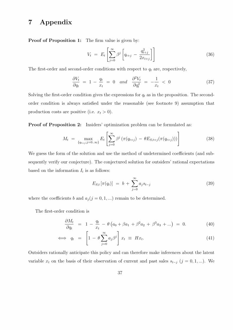
7 Appendix

Proof of Proposition 1: The firm value is given by:

Vt = Et

[∞∑j=0

βj[qt+j −

q2t+j

2xt+j

]](36)

The first-order and second-order conditions with respect to qt are, respectively,

∂Vt∂qt

= 1 − qtxt

= 0 and∂2Vt∂q2

t

= − 1

xt< 0 (37)

Solving the first-order condition gives the expressions for qt as in the proposition. The second-

order condition is always satisfied under the reasonable (see footnote 9) assumption that

production costs are positive (i.e. xt > 0).

Proof of Proposition 2: Insiders’ optimization problem can be formulated as:

Mt = max{qt+j ;j=0..∞}

Et

[∞∑j=0

βj (π(qt+j) − θES,t+j(π(qt+j)))

](38)

We guess the form of the solution and use the method of undetermined coefficients (and sub-

sequently verify our conjecture). The conjectured solution for outsiders’ rational expectations

based on the information It is as follows:

ES,t [π(qt)] = b +∞∑j=0

ajst−j (39)

where the coefficients b and aj(j = 0, 1, ...) remain to be determined.

The first-order condition is

∂Mt

∂qt= 1 − qt

xt− θ

(a0 + βa1 + β2a2 + β3a3 + ...

)= 0. (40)

⇐⇒ qt =

[1 − θ

∞∑j=0

ajβj

]xt ≡ Hxt. (41)

Outsiders rationally anticipate this policy and can therefore make inferences about the latent

variable xt on the basis of their observation of current and past sales st−j (j = 0, 1, ...). We

37

know that st = qt + εt. This measurement equation can be combined with the state equation

(8) to make inferences about xt on the basis of current and past observations of st. This, in

turn, allows outsiders to form an estimate of realized income πt. It can be shown that the

Kalman filter is the optimal filter (in terms of minimizing the mean squared error) for the

type of problem we are considering (see Chui and Chen (1991)).

One can show (see Chui and Chen (1991), p78) that the error of the steady state estimator,

xt − xt, is normally distributed with zero mean and variance P , i.e., ES,t[xt − xt] = 0 and

ES,t[(xt − xt)2] = P , or p(xt|It) ∼ N(xt, P ), where xt is given by:

xt = Axt−1 +B + K [st − H (Axt−1 +B)] = (Axt−1 +B)λ + Kst (42)

=Bλ

1− λA+ K

∞∑j=0

λjAjst−j , where (43)

λ ≡ (1 − KH) and K ≡ H P

H2P + R(44)

and where P is the positive root of the equation (20). K is called the “Kalman gain” and it

plays a crucial role in the updating process.29 Using the conjectured solution for qt it follows

that outsiders’ estimate of income at time t is given by:

ES,t[πt] = ESt

[Hxt −

H2xt2

]=

(H − H2

2

)xt (45)

=

(H − H2

2

)[λB

1− λA+ K

∞∑j=0

(λA)j st−j

](46)

= b +∞∑j=0

ajst−j (47)

where the last step follows from our original conjecture given by equation (39). This allows

29If there is little prior history regarding sales st then Kt itself will vary over time because Pt, the variance of

the estimation error, initially fluctuates over time. Once a sufficient number of observations have occurred Pt,

and therefore Kt, converge to their stationary level P and K. A sufficient condition for the filter to converge

is that λ A < 1. The order of convergence is geometric (see Chui and Chen, 1991, Theorem 6.1 on Page 88).

38

us to identify the coefficients b and aj:

b =

(H − H2

2

)[λB

1− λA

](48)

aj =

(H − H2

2

)K (λA)j (49)

For this to be a rational expectations equilibrium it has to be that (see equation (41)):

H = 1 − θ

∞∑j=0

ajβj = 1 −

θ(H − H2

2

)K

1− βλA(50)

Simplifying gives the condition forH in the proposition. Fixing outsiders’ beliefs (i.e. ES,t[π(qt+j)] =(H − H2

2

)xt+j ≡ hxt+j) and solving for insiders’ optimal production it follows from (11)–

(13) that insiders’ output strategy is a fixed point. One can also immediately verify that the

second order condition for a maximum is satisfied (assuming xt is positive).

Finally, we calculate the expected value and variance of the estimate’s error: πt − πt.

We make use of the result that the error with respect to the steady state estimator for xt is

normally distributed with zero mean and variance P . Hence,

ES,t[πt − πt] = ES,t [h(xt − xt)] = 0 (51)

ES,t[(πt − πt)2] = ES,t

[h2(xt − xt)

2]

= h2 P (52)

Proof of Proposition 3: Actual income under insiders’ production policy is given by:

πt = qt −q2t

2xt= hxt (53)

We know from the proof of proposition 2 that πt = ES,t[πt] = b +∑∞

j=0 ajst−j (where the

values for b and aj are defined there). Lagging this expression by one period, it follows that

πt − λAπt−1 = hKst + hλB. Substituting this expression into the target adjustment model

(21) gives:

λA πt−1 + Khst + hλB = πt−1 + (1− λA)π∗t − πt−1 + λAπt−1 (54)

Simplifying and solving for π∗t gives equation (23).

39

Proof of Proposition 4: Assume that x0 ≡ ES,0[x0] = x0 when the equity is issued. As

a result, outsiders and insiders predict the same future path for xt at time t = 0. Indeed,

ES,0[x1] = Ax0 +B = E0[x1]; ES,0[x2] = A2x0 + AB +B = E0[x2]; ES,0[x3] = ....

Therefore, insiders and outsiders value the company identically. This firm value is

V0 = E0[∞∑j=0

βjπj] = hx0 + β (hAx0 + hB) + β2(hA2x0 + hAB + hB

)+ ... (55)

= hx0

(1 + βA + β2A2 + β3A3 + ...

)+ hBβ

(1 + βA + β2A2 + β3A3 + ...

)+hBβ2

(1 + βA + β2A2 + ...

)+

hBβ3

1− βA+

hBβ4

1− βA+ ...

=h

(1− βA)

(x0 +

Bβ

1− β

). ♦ (56)

Proof of Proposition 5: The valuation equation for St follows immediately from propo-

sition 4 (by substituting x0 and β by xt and β(1 − δ), respectively). The derivation of the

equilibrium value for H is as given in the proof to proposition 2 but with θ replaced by

θ(

1− δ1−β(1−δ)A

).

References

Acharya, V., S. C. Myers, and R. G. Rajan (2011): “The Internal Governance of Firms,”

Journal of Finance, 66, 689–720.

Amihud, Y., J. Y. Kamin, and J. Ronen (1983): “Managerialism and Ownerism in Risk-Return

Preferences,” Journal of Banking and Finance, 7(2), 189–196.

Asker, J. W., J. Farre-Mensa, and A. Ljungqvist (2012): “Comparing the Investment Be-

havior of Public and Private Firms,” SSRN Working Paper 1603484.

Baber, W. R., P. M. Fairfield, and J. A. Haggard (1991): “The Effect of Concern about

Reported Income on Discretionary Spending Decisions: The Case of Research and Development,”

The Accounting Review, 66, 818–829.

40

Bagnoli, M., and S. G. Watts (2010): “Oligopoly, Disclosure and Earnings Management,” The

Accounting Review, 85(4), 1191–1214.

Baron, D. P., and D. Besanko (1987): “Commitment and Fairness in a Dynamic Regulatory

Relationship,” Review of Economic Studies, 54(3), 413–436.

Bebchuk, L. A., and L. A. Stole (1993): “Do Short-Term Objectives Lead to Under- or Over-

investment in Long-Term Projects,” Journal of Finance, 48(2), 719–729.

Bhojraj, S., P. Hribar, M. Picconi, and J. McInnis (2009): “Making Sense of Cents: An

Examination of Firms That Marginally Miss or Beat Analyst Forecasts,” Journal of Finance,

64(5), 2361–2388.

Chui, C. K., and G. Chen (1991): Kalman Filtering with Real-Time Applications. Springer-Verlag,

Heidelberg.

Daniel, N. D., D. J. Denis, and L. Naveen (2012): “Sources of Financial Flexibility: Evidence

from Cash Flow Shortfalls,” Mimeo, Temple University.

DeFond, M. L., and C. W. Park (1997): “Smoothing Income in Anticipation of Future Earnings,”

Journal of Accounting and Economics, 23(2), 115–139.

Dye, R. A. (1988): “Earnings Management in an Overlapping Generations Model,” Journal of

Accounting Research, 26, 195–235.

Fluck, Z. (1998): “Optimal Financial Contracting: Debt versus Outside Equity,” Review of Finan-

cial Studies, 11(2), 383–419.

(1999): “The Dynamics of the Management-Shareholder Conflict,” Review of Financial

Studies, 12, 379–404.

Freixas, X., R. Guesnerie, and J. Tirole (1985): “Planning under Incomplete Information and

the Ratchet Effect,” The Review of Economic Studies, 52(2), 173–191.

Fudenberg, D., and J. Tirole (1995): “A Theory of Income and Dividend Smoothing Based on

Incumbency Rents,” Journal of Political Economy, 103(1), 75–93.

41

Gal-Or, E. (1987): “First Mover Disadvantages with Private Information,” Review of Economic

Studies, 54(2), 279–292.

Gao, H., M. Lemmon, and K. Li (2000): “A Comparison of CEO Pay in Public and Private U.S.

Firms,” working paper, University of British Columbia.

Gelb, A. (1974): Applied Optimal Estimation. MIT Press, Cambridge (MA).

Gibbons, R., and K. J. Murphy (1992): “Optimal Incentive Contracts in the Presence of Career

Concerns: Theory and Evidence,” Journal of Political Economy, 100, 468–505.

Goel, A. M., and A. V. Thakor (2003): “Why Do Firms Smooth Earnings?,” Journal of Busi-

ness, 76(1), 151–192.

Graham, J. R. (2003): “Taxes and Corporate Finance: A Review,” Review of Financial Studies,

16(4), 1075–1129.

Graham, J. R., C. R. Harvey, and S. Rajgopal (2005): “The Economic Implications of Cor-

porate Financial Reporting,” Journal of Accounting and Economics, 40, 3–73.

Grossman, S. J. (1976): “On the Efficiency of Competitive Stock Markets Where Traders Have

Diverse Information,” Journal of Finance, 31(2), 573–584.

Holmstrom, B. (1999): “Managerial Incentive Problems: A Dynamic Perspective,” The Review of

Economic Studies, 66(1), 169–182.

Indjejikian, R., and D. Nanda (1999): “Dynamic Incentives and Responsibility Accounting,”

Journal of Accounting and Economics, 27(2), 177–201.

Jin, L., and S. C. Myers (2006): “R2 around the World: New Theory and New Tests,” Journal

of Financial Economics, 79, 257–292.

Kamin, J. Y., and J. Ronen (1978): “Smoothing of Income Numbers: Some Empirical Evi-

dence on Systematic Differences Among Management-Controlled and Owner-Controlled Firms,”

Accounting, Organizations and Society, 3(2), 141–157.

Kanodia, C., and A. Mukherji (1996): “Real Effects of Separating Investment and Operating

Cash Flows,” Review of Accounting Studies, 1(1), 51–71.

42

King, R. G., and R. Levine (1993): “Finance and Growth: Schumpeter Might Be Right,” Quar-

terly Journal of Economics, 153, 717–738.

La Porta, R., F. Lopes-De-Silanes, A. Shleifer, and R. Vishny (1998): “Law and Finance,”

Journal of Political Economy, 106, 1113–1155.

Laffont, J., and J. Tirole (1988): “The Dynamics of Incentive Contracts,” Econometrica, 56(3),

1153–1175.

Lambert, R. A. (1984): “Income Smoothing as Rational Equilibrium Behavior,” Accounting Re-

view, 59, 604–618.

Lambrecht, B. M., and S. C. Myers (2007): “A Theory of Takeovers and Disinvestment,”

Journal of Finance, 62(2), 809–845.

(2008): “Debt and Managerial Rents in a Real-Options Model of the Firm,” Journal of

Financial Economics, 89(2), 209–231.

(2012): “A Lintner Model of Payout and Managerial Rents,” Journal of Finance, 67(5),

1761–1810.

Lieber, Z., E. Melnick, and J. Ronen (1983): “The Filtering of Transitory Noise in Earnings

Numbers,” Journal of Forecasting, 2, 331–350.

Lintner, J. (1956): “Distribution of Incomes of Corporations among Dividends, Retained Earnings,

and Taxes,” American Economic Review, 46, 97–113.

McConnell, J., and H. Servaes (1990): “Additional Evidence on Equity Ownership and Corpo-

rate Value,” Journal of Financial Economics, 27, 595–612.

Mergenthaler, R. D., S. Rajgopal, and S. Srinivasan (2012): “CEO and CFO Career Penal-

ties to Missing Quarterly Analysts Forecasts,” SSRN working paper 1152421.

Michaely, R., and M. R. Roberts (2012): “Corporate Dividend Policies: Lessons from Private

Firms,” Review of Financial Studies, 25(3), 711–746.

Milgrom, P. R., and J. Roberts (1982): “Limit Pricing and Entry Under Incomplete Information:

An Equilibrium Analysis,” Econometrica, 50, 443–460.

43

Morck, R., A. Shleifer, and R. W. Vishny (1988): “Management Ownership and Market

Valuation,” Journal of Financial Economics, 20, 293–315.

Myers, S. C. (2000): “Outside Equity,” Journal of Finance, 55(3), 1005–1037.

Myers, S. C., and N. S. Majluf (1984): “Corporate Financing and Investment Decisions when

Firms have Information that Investors do not have,” Journal of Financial Economics, 13, 187–221.

Prencipe, A., S. Bar-Yosef, P. Mazzola, and L. Pozza (2011): “Income Smoothing in

Family-controlled Companies: Evidence from Italy,” Corporate Governance: An International

Review, 19(6), 529–546.

Rajan, R. G., and L. Zingales (1998): “Financial Dependence and Growth,” American Economic

Review, 88, 559–586.

Riordan, M. (1985): “Imperfect Information and Dynamic Conjectural Variation,” The Rand Jour-

nal of Economics, 16, 41–50.

Ronen, J., and S. Sadan (1981): Smoothing Income Numbers: Objectives, Means, and Implica-

tions. Addison-Wesley Publishing Company, Reading, Mass.

Roychowdhury, S. (2006): “Earnings Management through Real Activities Manipulation,” Jour-

nal of Accounting and Economics, 42(3), 335–370.

Stein, J. (1989): “Efficient Capital Markets, Inefficient Firms: A Model of Myopic Corporate

Behavior,” Quarterly Journal of Economics, 104(4), 655–669.

Trueman, B., and S. Titman (1988): “An Explanation for Accounting Income Smoothing,”

Journal of Accounting Research, 26, 127–139.

Tucker, J. W., and P. A. Zarowin (2006): “Does Income Smoothing Improve Earnings Infor-

mativeness?,” The Accounting Review, 81(1), 251–270.

Weitzman, M. L. (1980): “The Ratchet Principle and Performance Incentives,” The Bell Journal

of Economics, 11(1), 302–308.

44

Figure 1: Production efficiency

The figure examines how production efficiency is affected by the variance of measurement errors (R), the variance

of the latent cost variable xt (Q), the autocorrelation at lag one of the latent cost variable (A) and outsiders’

real ownership stake (θ). Production efficiency is measured by comparing unconditional mean output (E(qt)) and

unconditional mean income (E(πt)) relative to their first-best level. The baseline parameter values used to generate

the figures in this paper are: A = 0.9, B = 10, Q = 5, R = 1, β = 0.95 and θ = 0.8.

Figure 2: Total firm value and outside equity value

The figure plots the total initial firm value V0 (panel A) and outside equity value S0 (panel B) as a function of

outsiders’ real ownership stake (θ) for three different levels of audited disclosure quality (κ). The inverted U-shaped

curves in panel B are the so-called “outside equity Laffer curves”. The baseline parameter values used to generate

the figure are the same as before, i.e., A = 0.9, B = 10, Q = 5, R = 1, β = 0.95 and θ = 0.8.