A Takagi–Sugeno model with fuzzy inputs viewed from multidimensional interval analysis

Fuzzy Sets and Systems 135 (2003) 39–61www.elsevier.com/locate/fss

A Takagi–Sugeno model with fuzzy inputs viewedfrom multidimensional interval analysis

Felipe Fern'andez ∗, Julio Guti'errez

Dep. Tecnolog��a Fot�onica, Facultad de Inform�atica, Universidad Polit�ecnica de Madrid, 28660 Madrid, Spain

Abstract

Takagi–Sugeno (T–S) fuzzy systems have been successfully applied to a wide range of problems and havedemonstrated signi,cant advantages in nonlinear control. This paper presents a fuzzi,ed T–S interpolation–approximation system mainly based on the speci,cation of a multidimensional crisp partition that de,nesthe corresponding local regions (multidimensional intervals) where the corresponding rules apply, the relatedoutput functions and a reduced set of global fuzzy parameters. These fuzzy parameters capture the di.erentuncertainties of a fuzzy system: imprecision of inputs, vagueness of antecedent linguistic labels and smooth-ness requirements of outputs. This approach makes easier the design of a zero-order product–sum T–S systemwith fuzzi,ed inputs, fuzzi,ed antecedent crisp partition, and outputs with an additional spatial output ,lter.Convolution operations applied on an equalized and normalized input domain are considered to specify thecorresponding fuzzi,cation of a crisp partition. The kernels of these convolutions are even B-spline func-tions of order n, constructed from a n-fold convolution of an even interval characteristic function. We use acorrectness-preserving transformation to simplify the output computation: a global transformation of impreci-sion of inputs, vagueness of antecedent terms and smoothness requirements of outputs into a set of o.-lineconvolution operations applied to the corresponding antecedent crisp partition. By this method a fuzzi,edzero-order T–S system de,ned on a multidimensional crisp partition is directly transformed into a multidi-mensional spline interpolator–approximator by means of fuzzy operations and an equalization–normalizationof the corresponding input domain. c© 2002 Elsevier Science B.V. All rights reserved.

1. Introduction

A control system where one chooses from a set of prede,ned linear controllers each havingbeen tuned for a particular operating region, is commonly referred to as gain scheduling. In thisapproach, several operating points covering the range of the system dynamics are selected, and

∗ Corresponding author. Tel.: +34-91-3367372.E-mail addresses: [email protected] (F. Fern'andez), jgr@dtf.,.upm.es (J. Guti'errez).

0165-0114/03/$ - see front matter c© 2002 Elsevier Science B.V. All rights reserved.PII: S0165-0114(02)00249-X

40 F. Fern�andez, J. Guti�errez / Fuzzy Sets and Systems 135 (2003) 39–61

for each operating points a linear time invariant approximation of the original nonlinear system isconstructed. Finally, a linear controller for each linearized system is designed. In between operatingpoints, the linear controller parameters are interpolated (or scheduled).

In 1985, Takagi and Sugeno generalized the previous nonlinear model using fuzzy sets and fuzzylogic, and described nonlinear systems using a set of conditional fuzzy rules or local models, witheach one being valid in a particular operating fuzzy region determined by the corresponding speci,-cation of antecedent membership functions. A conditional part or antecedent de,nes each operatingregion. The consequent part of each rule is an analytical expression describing the correspondinglocal model. These collections of local models together with a merging procedure are the basic in-gredients of Takagi–Sugeno (T–S) model. In general the aggregation procedure consists of a convexcombination of the corresponding local models de,ned in the corresponding fuzzy region.

Standard T–S systems provide a formal method for modelling vagueness of local regions associatedto the input domain and an output merging procedure of the corresponding fuzzy rules.

This paper introduces a MISO zero-order T–S system considering fuzzi,ed inputs variables, fuzzi-,ed interval terms and an additional spatially smoothing output ,lter (fuzzi,ed output). All fuzzi-,cation transforms here referred are derived as spatial convolution=,lter operations. The kernels ofall these ,lters are B-spline functions.

As in interval analysis [10,11], the inaccuracy or uncertainty of input variables is initially mod-elled by an interval number that represents the range of possible values with a closed set. A moregeneral approach here considered specify this uncertainty by means of a n-fold convolution ofthe characteristic function of an even interval that provides a B-spline fuzzi,cation function oforder n.

Nowadays, B-spline techniques represents one of the most important tools in CAD=CAM that havebeen extensively applied in modelling shape curves and surfaces of many practical systems [5].

Recently, splines have also been used to solve the problem of specifying systems with smooth-ness requirements for neuro-fuzzy network modelling and control (for example [13–16]). In theseapproaches, uniform and nonuniform B-spline functions are used for de,ning membership functionsof fuzzy systems, but to the best of our knowledge, the de,nitions of these B-splines are not directlyderived from fuzzy operations, and the models considered have less expressive power to characterizethe di.erent uncertainties of a fuzzy system.

In [6] is considered an eHcient computation of fuzzy propositions with fuzzi,ed inputs usingmax–min convolution operation. This approach has the disadvantage that the corresponding o.-linefuzzi,cation function does not preserve the corresponding partition of unity of the correspondingantecedent terms. In our previous paper [7], we introduced a product–sum uniform fuzzi,cationconvolution that preserves the partition of unity condition.

In the present paper we generalize the previous approaches and introduce a new equalization–normalization function on each input variable to specify and implement fuzzi,ed fuzzy systemswith uniform and nonuniform fuzziness. This input function here considered allows simplifying thespeci,cation of a nonuniform fuzzi,cation of the antecedent terms.

The input and antecedent term fuzzi,cation functions and the kernel of output ,lter considered aremultivariate tensor-product B-spline functions. The antecedent linguistic terms obtained are multivari-ate tensor-product nonuniform spline fuzzy partitions de,ned from crisp partitions with an additionalfuzzi,cation transformation, accomplished on an equalized input domain. The obtained partitions ofunity are derived as a result of uniform and nonuniform fuzzi,cation transforms.

F. Fern�andez, J. Guti�errez / Fuzzy Sets and Systems 135 (2003) 39–61 41

Fig. 1. Transformation by fuzzi,cation convolution of standard intervals and partitions into fuzzy intervals and fuzzypartitions.

A uni,ed approach is used to model three types of uncertainty associated with the description ofa fuzzy system: uniform imprecision of each input, nonuniform vagueness of each antecedent termspartition and uniform output smoothness requirements.

The corresponding uncertainties are modelled by the convolution=,lter operations: input fuzzi,ca-tion, antecedent term fuzzi,cation and spatial output ,ltering.

The main motivation of the fuzzi,ed T–S model presented is to simplify the description and im-plementation of a fuzzy system by means of an orthogonal decomposition of a fuzzy model intotwo major parts: a crisp and accurate component, and a fuzzy component. The fuzzi,cation convo-lution is used as a bridge between intervals and fuzzy intervals. Thus, a fuzzy partition speci,cationis divided into two factors: crisp partition and uncertainty speci,cation (Fig. 1). This crisp–fuzzybreaking down is in a sense analogous to the standard splitting used in classical engineering to copewith imprecision, errors and noise.

In this paper, we have initially considered only intervals as antecedent linguistic terms and wehave reduced the kernel of convolutions=,lters used to even B-spline function [5]. This selectiondoes not limit too much the expressive power of the model, simpli,es very much the correspondingspeci,cation and analysis process, and provides a rich set of interesting properties to the fuzzyinterpolation–approximation system considered.

The rest of the paper is organized as follows: Section 2 reviews some general de,nitions andterminology on multidimensional fuzzy sets and fuzzy partitions; the multidimensional fuzzi,cationtransform is introduced in Section 3; Sections 4 and 5 introduce the concepts of multidimensionalF-spline partitions and multidimensional equalized F-spline partitions; Section 6 describes a fuzzi,edzero-order T–S interpolation-approximation system and presents an o.-line correctness preservingtransformation used for the eHcient computation of the corresponding system; in Section 7 twoapplication examples are shown; and Section 8 concludes the work.

2. Multidimensional intervals and multidimensional fuzzy intervals

For interest of ulterior development, this section summarizes some general terminology and de,-nitions used in this paper. We also review some related standard concepts required from fuzzy sets[1,8] and interval analysis [10], and introduce new ones on fuzzy sets, fuzzy intervals and fuzzypartitions.


• A n-multidimensional interval [a; b] determined by the endpoints a=(a1; a2; : : : ; an) and b=(b1; b2; : : : ; bn)∈Rn (a6b), can be de,ned by its characteristic function as a mapping I :Rn→{0; 1}

I(u) = {(u ∈ Rn | ak 6 uk 6 bk ; 1 6 k 6 n) → 1; 0} = 1[a; b]:

• The set of corners of a multidimensional interval [a; b] is given by

Cor([a; b]) = {u ∈ Rn | uk = ak or uk = bk ; 1 6 k 6 n}:• The set of widths of a multidimensional interval [a; b] is de,ned as

Width([a; b]) = {w1; w2; : : : ; wn} = {b1 − a1; b2 − a2; : : : ; bn − an}:• A multidimensional fuzzy set A can be de,ned as a function of the form

A : Rn → [0; 1]:

For convenience of ulterior development, we introduce the nonstandard concept of S-fuzzy set [7](signal fuzzy set) A de,ned as a function

A : Rn → [0;∞):

This extension is mainly justi,ed as a consequence of using fuzzy techniques as good universalapproximators of general systems and in order to allow common signal processing de,nitions andtransformations.

• A fuzzy set A is normal when Height(A)=1.• A normal convex fuzzy set is usually called in the literature fuzzy number, L–R fuzzy number

or fuzzy interval [8]. In this paper, for a more general consideration of fuzzy numbers or fuzzyintervals we relax the normality condition and only maintain the convexity constraint.

• To accomplish general functional transformations, we introduce the nonnormal class (into theS-fuzzy sets and S-fuzzy intervals) to designate those ones with Height(A) =1 (subnormal when06Height(A)¡1 and supernormal when Height(A)¿1).

We also recall the following standard concepts [8]. These concepts are valid for one-dimensionaldomains (U=R1) or for n-multidimensional domains (U=Rn).

• Cardinality of a fuzzy interval A, on a discrete domain U , is de,ned by

|A| =∑u∈U

A(u):

• Area of a fuzzy interval A, on a continuous domain U , is de,ned by

|A| =∫UA(u) du:

In this paper we name a S-fuzzy set C-normal when its area or cardinality is |A|=1, and weusually substitute the normality condition of fuzzy inputs (height=1) by the C-normality condition(Area=1).


• Core of a fuzzy interval A is the interval of U , de,ned by

Core(A) = {u |A(u) = 1; u ∈ U}:• Any set that is not crisp has some degree of fuzziness that results from the imprecision of its

boundaries [6,8]. For measuring fuzziness of a fuzzy set, we can use the function fuz to expressthe lack of distinction between the membership A(u) and its complement 1 − A(u)

fuz(A) =∫

Supp(A)(1 − 2 |A(u) − 0:5|) du:

For example, the fuzziness of a normal trapezoidal fuzzy interval A is [6]

fuz(A) = (�+ �)=2;

where � and � are the bases length of the corresponding left and right rectangular triangles.• A set of M scalar linguistic terms P={A1; A2; : : : ; AM} is de,ned in the domain U of a given

scalar variable u. It is generally required that the linguistic terms satisfy the property of coverage,i.e. for each domain element is assigned at least one fuzzy set Aj with nonzero membership degree.

In practical applications, the linguistic terms are generally constrained to be normal or subnormalfuzzy intervals. Also the model here considered, and presently in many other fuzzy control models[1,14,16], imposes stronger conditions on the linguistic terms used:Ruspini-partition of unity of a domain U is de,ned by the following constraints:

0 6 Aj(u) 6 1 ∀u ∈ U; 1 6 j 6 M;

M∑j=1

Aj(u) = 1 ∀u ∈ U;

∑u∈U

Aj(u)¿0; 1 6 j 6 M:

First equation is the standard membership constraint. Second equation means that for each u,the sum of all membership degrees Aj(u) equals one. Third equation implies that none of the fuzzysets Aj(u) is empty. This fuzzy segmentation of domain U is also called fuzzy partition [1,8].A hard or crisp partition {Aj} can be considered as a particular case: Aj(u)∈{0; 1}.

• A knot sequence T={(t0; t1; : : : ; tk ; : : : ; tm) | (a= t0¡t1¡ · · ·¡tk¡ · · ·¡tm=b)} with [a; b]∈U ,de,nes a scalar crisp partition P, determined by a set of M intervals

P(u) = {I0; I1; : : : ; Ik ; : : : ; Im−1} = {1[t0; t1); 1[t1; t2); : : : ; 1[tk ; tk+1); : : : ; 1[tm−1; tm]}:• A crisp partition is called uniform when all its intervals have the same width.• An equalization–normalization function of a crisp partition P is de,ned in this paper as a mono-

tonic continuous function E :U→UN that transforms the ordered knots sequence T=(t0; (t0 + t1)=2; : : : ; (tk + tk+1)=2; : : : ; (tm−1 + tm)=2; tm) de,ned on a domain U , into the knots sequence TN=(0;12 ; : : : ; k + 1

2 ; : : : ; m− 12 ; m) de,ned on the corresponding equalized–normalized domain UN .


A22 A22

A12

u1

u2

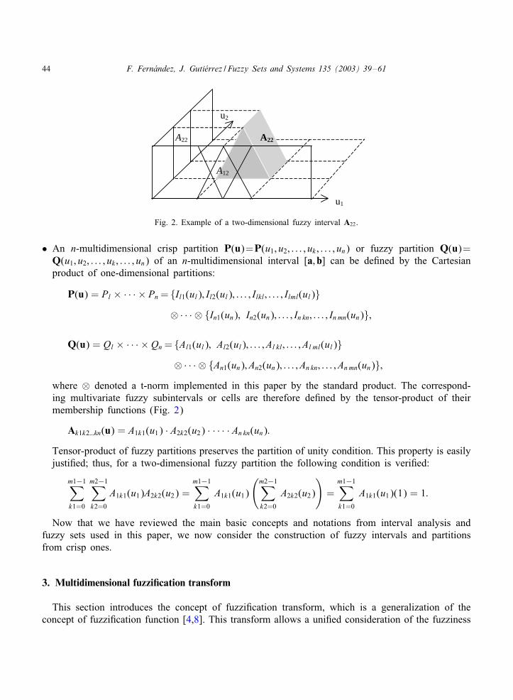
Fig. 2. Example of a two-dimensional fuzzy interval A22.

• An n-multidimensional crisp partition P(u)=P(u1; u2; : : : ; uk ; : : : ; un) or fuzzy partition Q(u)=Q(u1; u2; : : : ; uk ; : : : ; un) of an n-multidimensional interval [a; b] can be de,ned by the Cartesianproduct of one-dimensional partitions:

P(u) = Pl × · · · × Pn = {Il1(ul); Il2(ul); : : : ; Ilkl; : : : ; Ilml(ul)}⊗ · · · ⊗ {In1(un); In2(un); : : : ; In kn; : : : ; In mn(un)};

Q(u) = Ql × · · · × Qn = {Al1(ul); Al2(ul); : : : ; Al kl; : : : ; Al ml(ul)}⊗ · · · ⊗ {An1(un); An2(un); : : : ; An kn; : : : ; Anmn(un)};

where ⊗ denoted a t-norm implemented in this paper by the standard product. The correspond-ing multivariate fuzzy subintervals or cells are therefore de,ned by the tensor-product of theirmembership functions (Fig. 2)

Ak1k2:::kn(u) = A1k1(u1) · A2k2(u2) · · · · · An kn(un):Tensor-product of fuzzy partitions preserves the partition of unity condition. This property is easilyjusti,ed; thus, for a two-dimensional fuzzy partition the following condition is veri,ed:

m1−1∑k1=0

m2−1∑k2=0

A1k1(u1)A2k2(u2) =m1−1∑k1=0

A1k1(u1)

(m2−1∑k2=0

A2k2(u2)

)=

m1−1∑k1=0

A1k1(u1)(1) = 1:

Now that we have reviewed the main basic concepts and notations from interval analysis andfuzzy sets used in this paper, we now consider the construction of fuzzy intervals and partitionsfrom crisp ones.

3. Multidimensional fuzzi�cation transform

This section introduces the concept of fuzzi,cation transform, which is a generalization of theconcept of fuzzi,cation function [4,8]. This transform allows a uni,ed consideration of the fuzziness


associated to the input variables and to the antecedent terms of a fuzzy system, and models thespatially smoothing output ,lter of a fuzzy interpolation–approximation system.

The scalar uniform fuzzi,cation transform F is a spatially or shift invariant transformation thatapplies an even fuzzi,cation function ! (even C-normal S-fuzzy number) onto a fuzzy number f(normal or subnormal), de,ned on a continuous domain U ; and gives a new fuzzy number f#

de,ned by means of the following cross-correlation=convolution operation:

F!(f)(v) = !∗f(v) =∫Uf(u)!(u− v) du =

∫Uf(u)!(v− u) du = f#(v):

The scalar equalized fuzzi,cation transform applies the previous operation on an equalized–normalized domain UN . The related even fuzzi,cation function ! has the following form:

!v; E(u) = !(E(u) − E(v));

where E represents an additional domain-equalization monotonic function applied (de,ned in Sec-tion 2) and v represents the corresponding shift or translation variable. This scalar shift variantfuzzi,cation transform is de,ned by means of the following inner product operation de,ned on thenormalized domain UN

F!; E(f)(v) = 〈!v; E(u); f(E(u))〉 =∫Uf(E(u))!(E(u) − E(v)) dE(u):

These de,nitions are easily extended to the multidimensional case where U=Rn; C=(v1; v2; : : : ; vn)∈Rn, f :Rn→ [0; 1]; ! :Rn→ [0;∞) and E :Rn→ [0; m]

F!(f)(v) = 〈Lv(u); f(u)〉 =∫RN

f(u)L(u − v) du

F!; E(f)(v) = 〈Lv;E(u); f(E(u))〉 =∫RN

f(E(v))L(E(u) − E(v)) dE(u):

The multidimensional fuzzi,cation function !(u) transforms therefore, in general, the fuzzinessof a multivariate function f(u) in whatever spatial direction. Most often, however, these multi-dimensional functions are represented in a decomposed simple form, and they are de,ned as atensor-product of their individual components:

!(u) = !1(u1)!2(u2) · · · · · !n(un);f(u) = f1(u1)f2(u2) · · · · · fn(un);E(u) = E(u1)E(u2); : : : ; ·E(un):

The corresponding implicit conjunctive partition divides the domain space into a grid of fuzzyhyperboxes (or multidimensional fuzzy subintervals).

A particular interesting case of fuzzi,cation convolution is the multidimensional Dirac impulsefuzzi,cation transform FT, normally called in the literature singleton fuzzi,cation transform

FT(f) = T ∗ f = f :

It is convenient to notice that the fuzzi,cation transform modi,es, in general, the support and coreof the corresponding fuzzy number, but it preserves the area and partition of unity condition as itis shown below.


On the contrary, if a max–min operation [3,15,6] is used to de,ne an analogous fuzzi,cationtransform (instead of sum–product), the corresponding operation modi,es the support but not thecore of the corresponding fuzzy number, and therefore it does not preserve the corresponding fuzzypartition.

Some important properties of the multidimensional fuzzi,cation transform are:

Partition of unity conservation. The fuzzi2cation transform of a multidimensional fuzzy partition({Aj} j=1::M) is another fuzzy partition, i.e. partitions of unity are closed under fuzzi2cationtransform

F!({Aj}) = ! ∗ {Aj} = {! ∗ Aj} = {A!j }:

Proof. It is a consequence of the distributive property of convolution operation

M∑j=1

! ∗ {Aj} = ! ∗ 1 = 1 ∀u ∈ U:

Area preservation. The fuzzi2cation transform preserves the area of a multidimensional fuzzy in-terval A

|A ∗ L| = |A|:

Proof. It is a consequence of the commutative and distributive property of integral operator∫UF!(A) dC=

∫U

∫U

L(u − C)A(u) du dC

=∫U

∫U

L(u − C)A(u) du = 1 · |A| ∀u ∈ U:

S-Fuzzy numbers are closed with respect fuzzi�cation transform. The set of multidimensional S-fuzzy intervals is closed under a uniform or equalized fuzzi2cation convolution.

Proof. Since fuzzi,cation ,ltering preserves the convexity property of a fuzzy intervals. Note thatthis property is also maintained for equalized monotonic fuzzi,cation transforms where the convexityproperty is also preserved.

Smoothness of a uniform fuzzi�cation transform. Uniform fuzzi2cation convolution is a smoothingtransform: If ! is spatially invariant and f and ! have smoothness of order m and n, respectively( f ∈Cm−2 and !∈Cn−2), then f ∗! has smoothness of order m+n ( f ∗!∈Cm+n−2). Smoothnessof order k means [2] that the derivative of order k of the function becomes impulsive, and thedi5erentiability class Ck is the space of functions that are k times continuously di5erentiable.

Proof. Since the order of Fourier transforms F of f ; ! and f ∗ ! are, respectively,

F( f ) = o(|s|−m); F(!) = o(|s|−n); F( f ∗ !) = o(|s|−(m+n))


hence the smoothness order of f ∗! is m+n (its (m+n)th derivative is impulsive) and consequentlyf ∗ ! belongs to the class Cm+n−2.

Smoothness of an equalized fuzzi�cation transform. In general the smoothness of an equalizedfuzzi2cation transform is dependent on the smoothness of the corresponding monotonic equalization–normalization function E. If f ; ! and E have smoothness of order m, n and p, respectively( f ∈Cm−2, !∈Cn−2 and w∈Cp−2), then f∗! has smoothness of order min(n+m; p) and thereforef ∗ !∈Cmin(n+m;p)−2.

Proof. It is a consequence of chain derivative rule of function composition.

A&ne invariance of a uniform fuzzi�cation transform. A7ne functions are 2xed points of a uni-form or equalized fuzzi2cation transform

F!(a · u + b) = !(u) ∗ (a · u + b) = a · u + b:

Proof. It is a consequence of the even and C-normal property of fuzzi,cation function !(u) used.In each position of the corresponding ,lter window, the corresponding average value, for two sym-metrical points of this window, is equal to the corresponding central value.

In this paper, to solve the bound problem associated to every convolution operation, a progressivelinear reduction of the kernel support of the fuzzi,cation function is applied in the proximity ofdomain bounds.

A null window width on the endpoints of the domain interval eliminates the boundary problemsof the average window used. This is a natural speci,cation in a fuzzy context, because usually inpractical applications, the extreme values of a variable can be ,xed without imprecision, and generallywe have no continuity constraints in the corresponding points of the output control surface.

We close this section with three interpretations of multidimensional fuzzi,cation convolution:1. As a cross-correlation between a multidimensional linguistic term A(·) and a multidimensional

fuzzy input variable X(·). This provides a measure of matching between the fuzzy term A and thefuzzy variable X :

X ∗ A(C) = 〈X(C);A(C)〉:The computation of a multidimensional fuzzy proposition (X is A) is greatly simpli,ed during theexecution time of the fuzzy algorithm when the fuzzi,cation transform is applied to the correspondinglinguistic label during the compilation time of the corresponding fuzzy algorithm

X ∗ A(C) = (Tx ∗ L) ∗ A(C) = Tx ∗ (! ∗ A)(C);

where Tx(C)= T(C− x) and x is the centre of the corresponding fuzzy input X=!x=(x ∗ !.2. As a multidimensional equalized fuzzi,cation operator with respect to a fuzzi,cation function

!(·), applied to a normalized interval I(·) de,ned on the domain UN .

! ∗ I (E(C)) = 〈!(E(u) − E(C)); I (E(u))〉:Thus, it is possible to control the global fuzziness degree of a fuzzy partition by means of thecorresponding fuzzi,cation operator.


3. As a spatial convolution ,ltering (multivariate lowpass ,lter) of a multivariate output signal zwith the multidimensional smoothing function !.

! ∗ z(C) = 〈!(C− u); z(u)〉:Thus, the lowpass multidimensional window function ! can be used for ,ltering the output z offuzzy system. This local averaging has the e.ect of suppressing the spatial high-frequency variationswhile preserving the basic shape of output surface z.

4. Multidimensional F-splines

The concepts of fuzzy intervals and fuzzy partitions are essential for the de,nition of a fuzzysystem, to divide the input space into fuzzy cells where the corresponding rules apply. The simplestinitial solution is a crisp grid partition, i.e. to divide each scalar input domain U=[a; b] into anordered set of p intervals de,ned by the knot sequence: a= t0¡t1¡ · · ·¡tj¡ · · ·¡tp=b, and assigneach interval to a crisp linguistic term I 1j de,ned by

I 1j (u) = *[tj; tj+1)(u) = 1[tj; tj+1)(u); j = 0; : : : ; p− 1;

where *A denotes, as usual, the characteristic function of a given crisp set A, and I 1j denotes aninterval or B-spline of order 1 (degree 0).

To transform this original crisp partition into a fuzzy one, a spatially invariant B-spline fuzzi,cationfunction N can be used. In one-dimensional space, the initial basis considered for fuzzi,cationfunctions is an even rectangular C-normal S-fuzzy number (of unit-area and support width w) N 1[w]

N 1[w](u) = (1=w)*[− 12w;

12w](u) = (1=w)1[− 1

2w;12w](u):

Applying a shift-invariant fuzzi,cation function N 1[w] to a crisp partition {I 1j } we obtain a newfuzzy partition {I 2j [w]} de,ned by the multiple convolution operation

{I 2j [w]}(u) = N 1[w] ∗ {I 1j }(u) = {N 1[w] ∗ I 1j }(u):The resulting trapezoidal or triangular fuzzy terms {I 2j [w]} are in general normal or subnormal

fuzzy intervals, and also form a partition of unity (fuzzy partition).An m-order B-spline fuzzi,cation function can be de,ned by the following recurrence equation,

for n=2; 3; : : :

Nm[w](u) = Nm−1[w] ∗ N 1[w](u) =∫ u+w=2

u−w=2Nm−1[w](v) dv:

In general, if an m-order B-spline fuzzi,cation function Nn[w] is convolved with a crisp partition{I 1j }

Nm[w] ∗ {I 1j }(u) = {Nm[w] ∗ I 1j }(u) = {Im+1j [w]}(u)

it gives a new fuzzy partition {Im+1j [w]}, which is a spline partition of order m + 1 or degree m,

which is a set of normal and subnormal fuzzy intervals. These fuzzy intervals are called in thispaper F-splines, and the corresponding fuzzy partitions are called F-spline partitions.


Notice that the fuzziness degree of a normal F-spline partition is spatially invariant, i.e. it has thesame value for all its components.

The parameters m (order) and w (original window width) of the considered B-spline determinethe support and shape of the corresponding convolution ,lter used and therefore the smoothness ofthe corresponding control surface obtained.

To solve the involved domain bound problem associated to every convolution operation, a varying(trapezoidal) kernel support length wu can be used

wu=2 = min((u− a);−(u− b); w=2):

This function of convolution kernel support length is zero in the corners of the corresponding domaininterval U=[a; b] and is constant between [a+ w=2; b−W=2].

Analogously, a multivariate B-spline fuzzi,cation function N(u) can be used to transform a mul-tivariate interval I1(u) into a fuzzy one Im+1(u). This multivariate B-spline can be de,ned as atensor-product of the univariate B-spline functions

Nm[w](u) = Nm1[w1](u1) · Nm2[w2](u2) · · · · · Nmn[w1](un):

The corresponding multidimensional F-spline partition {Im+1j [w]}(u), obtained from the tensor-

product crisp partition {I1j }(u)={I 1j1}(u1) · {I 1j2}(u2) · · · · · {I 1jn}(un), is given by the multiple

convolution operation

{Im+1j [w]}(u) = Nm[w] ∗ {I1

j }(u) = {Nm[w] ∗ I1j }(u):

An example of bivariate cubic F-spline: I(4;4)(0;3) [2, 2] (u1; u2) of order (4, 4) and original window

width [2, 2] is shown in Fig. 3.Some important properties of univariate F-splines considered, signi,cant for the design of T–S

systems, are shown below.

Properties. Each component of a multivariate tensor-product F-spline Im+1j [w](ui) of degree m and

(m+ 1)th-order has the following properties:

1. Support size: ‖supp(Im+1j [w])‖=‖supp(I 1j )‖ + m ∗ w

2. Core size: ‖core(Im+1j [w])‖= max(0; ‖core(I 1j )‖ − m ∗ w)

3. Continuity class: {Am+1j [w]}∈Cm−1 for m¿1

4. Symmetry: Am+1j [w] is symmetric with respect to the centre of A1

j

5. Polynomial form: Am+1j [w] are formed by piecewise polynomial functions of degree m.

Property 3 has special practical interest to determine the output continuity order (smoothness)of the T–S interpolation–approximation system considered. Notice that it is also possible to applyin cascade several uniform fuzzi,cation functions (multivariate tensor-product B-spline convolution,lters) with di.erent window support (w) and order (m), in order to characterize several spatiallyinvariant fuzziness of a MISO fuzzy system:

! = MINPUT ∗ MLABELS ∗ MOUTPUT = NmI[wIN] ∗ NmL[wLAB] ∗ NmO[wOUT]


Fig. 3. A bivariate F-spline of order (4, 4).

derived from the imprecision of input MINPUT, uniform vagueness of antecedents linguistic termsMLABELS and smoothness constraints of output MOUTPUT.

Therefore, the speci,cation of complex linguistic fuzzy partitions for controlling the smoothness ofa fuzzy system is not necessary in many cases, since the designer can factorize the uniform fuzzinessof a linguistic fuzzy partition. Thus, in regular fuzziness domains it is possible to specify crisplinguistic partitions and global fuzzi,cation parameters: m=(m1; m2; : : : ; mn) and w=(w1; w2; : : : ; wn),for the antecedents of the rules.

The next section mainly considers the problem of equalized fuzzy systems (spatially varyingfuzziness systems). Which is of practical interest specially when the sizes of intervals of the corre-sponding partition are very di.erent. In this case the uniform fuzziness speci,cation is not usuallyconvenient because it basically eliminates the e.ect of crisp linguistic labels with small support inthe corresponding control surface when a shift-invariant ,lter is applied.

5. Multidimensional equalized F-splines

The equalized F-spline considered in this paper, relaxed the fuzziness invariant property of thekernel used in the corresponding fuzzi,cation transform. Usually, it is convenient to have a fuzzypartition with a spatially varying fuzziness degree, approximately proportional to the width of thecorresponding initial intervals. For this purpose, a univariate nonuniform crisp partition P de,ned


U

UN

I0 I1 I2 I3 I4

t0 t1/2 t1 t3/2 t2 t5/2 t3 t7/2 t4 t9/2 t5

IE3

IE2

IE1

IE0

5

E

Fig. 4. A piecewise equalization–normalization function E of a crisp partition {Ii}i = 0::4 into the normalized uniformpartition {Ji}i = 0::4.

on a domain U=[t0; tm]

P(u) = {I 10 ; I 11 ; : : : ; I 1k ; : : : ; I 1m−1}(u) = {1[t0 ;t1); 1[t1 ;t2); : : : 1[tk ;tk+1); : : : ; 1[tm−1 ;tm)}(u)is transformed into a crisp equalized partition PN de,ned on a normalized domain UN=[0; m]

PN (E(u)) = {IE10 ; IE

11 ; : : : ; IE

1k ; : : : ; IE

1m−1}(E(u))

= {1[0; 1); 1[1; 2); : : : ; 1[k; k+1); : : : ; 1[m−1; m)}(E(u)):

The corresponding equalization–normalization of a crisp partition P, is given by a monotoniccontinuous function E :U→UN that transforms the sequence T=(t0; (t0 + t1)=2; : : : ; (tk + tk+1)=2; : : : ; (tm−1 + tm)=2; tm) de,ned on a domain U into the knots sequence TN=(0; 1

2 ; : : : ; k+ 12 ; : : : ; m−

12 ; m) de,ned on the corresponding normalized domain UN (see Fig. 4). This function is a piecewiseaHne function whose control points are placed in the middle points of the corresponding intervals.

The convolution is in this case applied to the obtained uniform crisp partition PN (E(u))={IE10 ;

IE11 ; : : : ; IE

1k ; : : : ; IE

1m}(E(u)) de,ned on the normalized domain UN . If an m-order B-spline fuzzi-

,cation function Nn[w] (E(u)) is convolved with a uniform crisp partition {IE1j }(E(u)), the new

uniform fuzzy partition on the domain UN is given by the multiple convolution

Nm[w] ∗ {IE1j }(E(u)) = {Nm[w] ∗ IE1

j }(E(u)) = {IEm+1j [w]}(E(u)):

The implied partition {Im+1j [w]}(u) on the domain U is obtained applying the inverse function

E−1 :UN→U . Therefore, in order to preserve the continuity order of the corresponding partition,an additional B-spline convolution ,lter Nm−1[w](E(u)) is also applied to the inverse equalizationfunction E−1.


The order and window width w of B-spline applied determines the general fuzziness of the cor-responding partition, and therefore the smoothness=interpolation degree of the corresponding fuzzycontrol surface.

Using the C-normal rectangular window ,lter several times or an equivalent B-spline fuzzi,cationtransform on the domain UN , it is possible to obtain easily an equalized F-spline partition for thecorresponding application. The resulting spline fuzzy terms {I m+1

j [w]}(u) also form a partition ofunity and can preserve the normal condition (height (Im+1

j [w](u)) = 1) if the suitable window widthw and B-spline order m is selected (Property 2 of Section 4), which is important, if we desire topreserve the interpolation condition of a T–S system, in the middle points of the corresponding fuzzyintervals.

The corresponding nonuniform F-spline partition on the original domain U : {Im+1j [w]} (u) has a

nonuniform fuzziness. This varying fuzziness partition is convenient when the corresponding initialpartition is not uniform, since a uniform fuzzi,cation ,ltering can partially eliminate the originalsmall crisp subintervals.

In Fig. 5 it is shown a univariate F-spline partition of order 4 and the corresponding inverseequalization function used to obtain this fuzzy partition. Notice that an additional B-spline ,lter hasbeen applied to the original aHne piecewise inverse equalization function, in order to preserve thecontinuity order of the involved membership functions.

Analogously a multivariate equalized F-spline partition {IEm+1j [w](E(u))} of order m + 1 is ob-

tained by means of the following tensor-product:

{IEm+1j [w](E(u))}= {Nm[w] ∗ IE1

j (u)}

= {Nm1[w1] ∗ IE1j1(E(u1)) · · · · · Nmn[wn] ∗ IE1

jn(E(un))};

where w = (w1; w2; : : : ; wn) and m = (m1; m2; : : : ; mn) represent, respectively, the initial support widthsand degree of the corresponding univariate B-splines applied.

6. Fuzzi�ed zero-order T–S interpolation–approximation system

A MISO zero-order T–S system rule can be speci,ed by a set of rp canonical rules {Rr} r= 1::rpas follows:

{Rr: If x1 is Ar1 and : : : and xN is ArN then z = br};

where x = (x1; x2; : : : ; xn)T ∈Rn are the inputs of the system and z ∈ R1 are the corresponding output,Arj are antecedent fuzzy numbers that belong to a fuzzy partition {Aij}, and br ∈R1 are constantvalues.

Using singleton fuzzi,er, product–sum inference and antecedent fuzzy partitions, the aggregatedfuzzy model can be written as

z =∑

R active

�r(x)br;


0

50

100

150

200

250

0 1 2 3 4 5

N2* *E-1

0

0.2

0.4

0.6

0.8

1

1.2

0 25 50 75 100 125 150 175 200 225 250

4I0

4I1

4I2

4I3

4I4

Fig. 5. Example of an inverse equalization function E ,ltered with N 2[0:6] and the corresponding equalized F-splinepartition of order 4 derived from the crisp partition de,ned by the knots sequence {0; 60; 70; 90; 150; 250}.

where �r(x) = �r1(x1)× �r2(x2)× · · ·× �rn(xn) is the ,ring degree of the rth rule, and �ri(xi) =Ari(xi)is the matching degree between the scalar variable xi and linguistic term Ari:, and Ractive is the setof active rules. The output values br are associated to each local model.

This T–S model has also a reduced equivalent multidimensional form, which is of interest for ourpurpose

{Rr: If x is Ar then z = br};where x= (x1; : : : ; xn) is the multivariate state variable and Ar =Ar1(x1)× · · ·×Arn(xn) is the mul-tivariate fuzzy number of the rth rule de,ned by means of the corresponding tensor-product, andbr is the involved output. The multidimensional fuzzy number Ar also de,nes a multidimensionalfuzzy cell of the corresponding fuzzy partition, where the local rule r is applied.

The T–S fuzzy system considered in this paper is a fuzzi,ed zero-order T–S model. Its rules areexpressed in conjunctive canonical form as

Rr: If X1 is IE!I1r1 and : : : and Xn is IE!Inrn then z = Br ;


Input x

∗

Fuzzy partition

Crisp partition ∗

T-S system

z = ∑α r br

br

α r

∗ Output

z

Output smoothness

Label fuzziness

Input imprecision

E E-1

Fig. 6. Fuzzi,ed zero-order T–S model.

where X1; : : : ; Xn are fuzzi,ed input variables that are univariate B-spline S-fuzzy numbers,IE!I1r1 ; : : : ; IE

! Inrn are univariate equalized F-splines and Br are fuzzi,ed outputs that are scaled mul-

tivariate B-splines. Moreover, each fuzzy term IE!Iiri (E(u)) belongs to the corresponding equalizedpartition of unity {IE!Iij }(E(u)). These equalized fuzzy partitions are fuzzi,ed versions of the originalequalized crisp partitions {IEij}.

This fuzzi,ed T–S model has also the following reduced equivalent multidimensional form

Rr: If X is IE!Ir then z = Br

where X =X1 × · · ·×Xn is a multivariate fuzzi,ed variable, IE!Xr = IE!I1r1 (u1) × · · · × IE!Inrn (un) is

a multivariate fuzzi,ed equalized interval term of the rth rule and Br =B1(u1)× · · · ×Bn(un) isa multivariate fuzzi,ed output term, de,ned by means of the corresponding tensor-products. Themultidimensional fuzzy number IE!r also de,nes a multidimensional fuzzy cell of the correspondingfuzzy partition, where the local rule r is applied.

In order to simplify and improve the speci,cation and implementation of a MISO T–S system, thefollowing additional developments are introduced, taking into account the fuzzi,cation transformspreviously de,ned (the basic structure of this model is shown in Fig. 6):

1. The multivariate fuzzy input variable X(u) is considered as the result of a uniform multivariateB-spline fuzzi,cation transform applied on the multivariate singleton input (x, in order to reOect theinputs imprecision

X(u) = !X ∗ (x(u) = Nmx[wx](u) ∗ (x(u);where Nmx[wx](u) is a uniform multivariate B-spline fuzzi,cation function applied to input (x(u).

2. The multivariate fuzzy terms IE!Ir are the result of an equalized multivariate fuzzi,cation trans-

form applied on a multivariate uniform crisp partition {IEr}, in order to contemplate the nonuniformvagueness (fuzziness) of the corresponding multivariate antecedent terms:

IE!Ir (E(u)) = !I ∗ IEr(E(u)) = NmI[wI](E(u)) ∗ IEr(E(u))

where NmI[wI](E(u)) is a multivariate B-spline fuzzi,cation function applied to the equalizedcrisp term IEr(E(u))(E(u)). The resulting fuzzy intervals are multivariate equalized F-splinesIEmI+1

r [wI](u).


Input x

Fuzzy partition

Crisp partition ∗

T-S system

z = ∑α r br

br

α r

Output z

Label fuzziness Input imprecision

Output smoothness

Fig. 7. Equivalent fuzzi,ed zero-order T–S model.

A more general alternative is to specify fuzzy partitions with two kind of fuzziness: uniform(derived by the convolution of the original crisp partition on the domain U ) and nonuniform (derivedby the posterior application of an equalized convolution on the normalized domain UN .

3. The output z of the system is the result of applying an additional uniform multivariate B-splinefuzzi,cation transform, in order to consider the corresponding smoothing constraints (multivariatelowpass ,lter) in the direction of each variable xi:

Br(u) = !Z ∗ (br(u) = Nmz[wz](u) ∗ (br(u);

where Nmz[wz](u) is a uniform multivariate B-spline ,lter convolution function applied to outputterm (br(u).

An aggregated fuzzi,cation transform that captures all the fuzzi,cations considered can be ob-tained, taking into account the additive nature of T–S system, the commutative and distributiveproperties of convolution operator, and the tensor-product structure of the antecedent terms of rules

!(u) = (!I(E(u)) ∗ (!Z(u) ∗ !X(u))(E(u))(u)):

This functional expression summarizes the di.erent convolution fuzzi,cations considered: in the orig-inal domain U (B-splines !X(u) and !Z(u)) and in the equalized domain UN (B-spline !I(E(u))).

Therefore, the rules Rr of an MISO system can be reduced to following equivalent form (Fig. 7)

Rr: If (x is ! ∗ Ir then z = br;

where (x(u)=((x1(u1)× · · · ×(xn(un)) is a multivariate Dirac impulse, 4(u)=!(u1)× · · · ×!(un)the referred multivariate fuzzi,cation function and Ir = Ir1(u1)× · · · × IrN (uN ) is the multivariateinterval of the rth rule.

This way, it is possible to apply an o.-line fuzzi,cation ! to the corresponding crisp partition {Ij}in order to simplify the corresponding on-line T–S system. This process can be executed during thecompilation time of the corresponding algorithm, in order to reduce dramatically the correspondingexecution time.


Using previous transformations, the output z of the fuzzy system can be computed in a similarform to a standard T–S fuzzy system with singleton input variables:

z =∑

R active

�r(x)br;

where �r(x) is the ,ring degree of the rth rule: �r(x) = �r1(x1)× �r2(x2)× · · ·× �rn(xn). Each factorof this tensor-product is determined by the membership degree of the transformed linguistic terms.The computation of output z does not use any division, since the tensor-product of fuzzy partitionsis also a partition of unity.

The main advantages of the fuzzi,ed ,rst order T–S system presented are:

• It simpli,es the speci,cation of a uniform fuzziness system by means of the crisp–fuzzy decom-position

Fuzzified zero-order T–S system

= Crisp zero-order T–S system + Fuzzification transform + Equalization function:

• The model has more expressive power because it incorporates into the model the nonuniformfuzziness of antecedent terms, the uniform imprecision of inputs and the uniform output smoothingrequirements.

• It is simple to compute because the fuzzi,ed T–S model it is transformed into a standard T–Sone using the referred canonical transformation. Thus, the compiled fuzzy algorithm does not useany convolution type operation during the execution time or any division for output evaluation.

The next section presents two application examples with the aim of showing the possibilities ofthe model considered.

7. Examples

In order to demonstrate practically the characteristics of the model presented, this section showstwo di.erent examples of fuzzy systems de,ned on one-dimensional and two-dimensional spaces.

The systems are speci,ed by means of a set of constant output functions de,ned on a grid crisppartition and a set of global fuzzy parameters. The following global fuzzy parameters are used tospecify fuzzi,cation functions applied:

• Input B-spline fuzzi,cation Nmxi[wxi](ui) for each domain Ui• Output B-spline fuzzi,cation Nmzi[wzi](ui) for each domain Ui• Antecedent term B-spline fuzzi,cation NmIi[wIi](Ei(ui)) for each normalized domain UNi.

The linguistic terms with nonuniform fuzziness are automatically computed using the equalizationfunctions previously de,ned. This way, the designer has usually enough Oexibility to specify thefuzzy part of a system, but without the necessity to indicate individually the fuzzy characteristics ofeach linguistic label used.


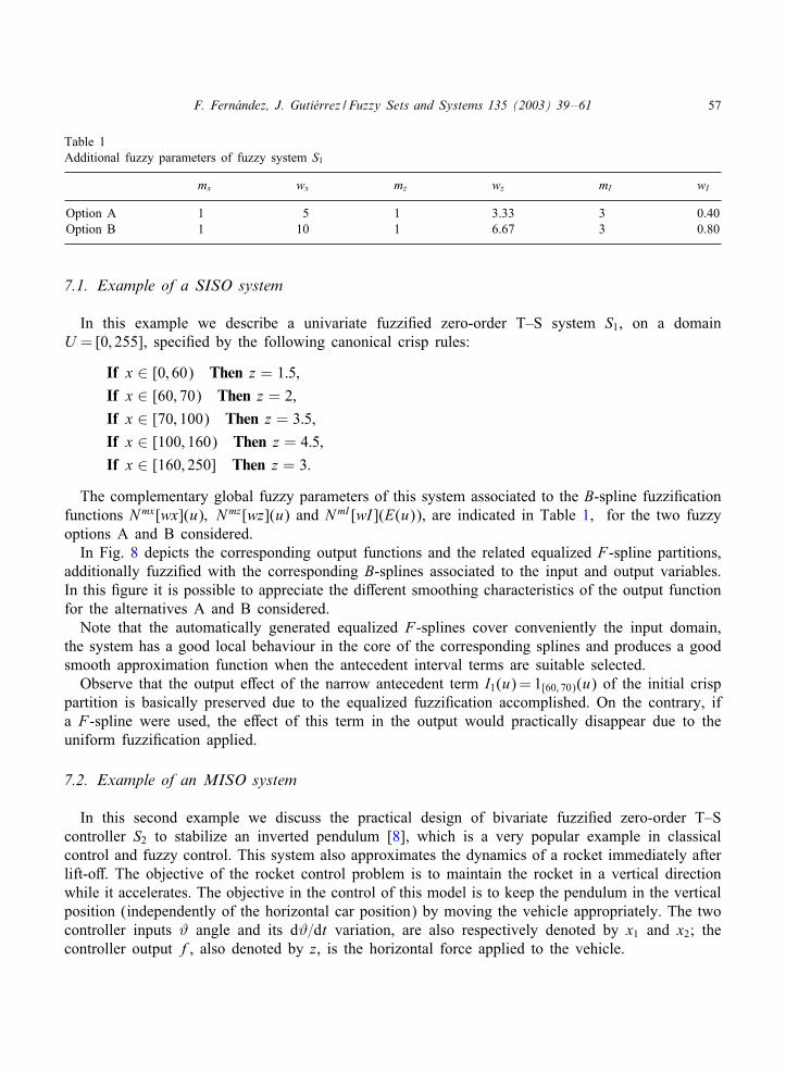
Table 1Additional fuzzy parameters of fuzzy system S1

mx wx mz wz mI wI

Option A 1 5 1 3.33 3 0.40Option B 1 10 1 6.67 3 0.80

7.1. Example of a SISO system

In this example we describe a univariate fuzzi,ed zero-order T–S system S1, on a domainU = [0; 255], speci,ed by the following canonical crisp rules:

If x ∈ [0; 60) Then z = 1:5;

If x ∈ [60; 70) Then z = 2;

If x ∈ [70; 100) Then z = 3:5;

If x ∈ [100; 160) Then z = 4:5;

If x ∈ [160; 250] Then z = 3:

The complementary global fuzzy parameters of this system associated to the B-spline fuzzi,cationfunctions Nmx[wx](u); Nmz[wz](u) and NmI [wI ](E(u)), are indicated in Table 1, for the two fuzzyoptions A and B considered.

In Fig. 8 depicts the corresponding output functions and the related equalized F-spline partitions,additionally fuzzi,ed with the corresponding B-splines associated to the input and output variables.In this ,gure it is possible to appreciate the di.erent smoothing characteristics of the output functionfor the alternatives A and B considered.

Note that the automatically generated equalized F-splines cover conveniently the input domain,the system has a good local behaviour in the core of the corresponding splines and produces a goodsmooth approximation function when the antecedent interval terms are suitable selected.

Observe that the output e.ect of the narrow antecedent term I1(u) = 1[60; 70)(u) of the initial crisppartition is basically preserved due to the equalized fuzzi,cation accomplished. On the contrary, ifa F-spline were used, the e.ect of this term in the output would practically disappear due to theuniform fuzzi,cation applied.

7.2. Example of an MISO system

In this second example we discuss the practical design of bivariate fuzzi,ed zero-order T–Scontroller S2 to stabilize an inverted pendulum [8], which is a very popular example in classicalcontrol and fuzzy control. This system also approximates the dynamics of a rocket immediately afterlift-o.. The objective of the rocket control problem is to maintain the rocket in a vertical directionwhile it accelerates. The objective in the control of this model is to keep the pendulum in the verticalposition (independently of the horizontal car position) by moving the vehicle appropriately. The twocontroller inputs # angle and its d#=dt variation, are also respectively denoted by x1 and x2; thecontroller output f, also denoted by z, is the horizontal force applied to the vehicle.


0

0.5

1

1.5

2

2.5

3

3.5

4

4.5

5

0 25 50 75 100 125 150 175 200 225 250

I0

I1

I2

I3

I4

z

Option A

0

0.5

1

1.5

2

2.5

3

3.5

4

4.5

0 25 50 75 100 125 150 175 200 225 250

I0

I1

I2

I3

I4

z

Option B

Fig. 8. Univariate fuzzi,ed zero-order T–S systems: options A and B.

We choose the following initial scaled variable domains

−4 6 #6 4;

−4 6 d#=dt 6 4;

−2 6 f 6 2:

Following Yamakawa experiments [8], we use the crisp conditional inference rules de,ned in Table 2.

The complementary global fuzzy parameters of this system associated to the bivariate B-splinefuzzi,cation functions Nmx[wx](u); Nmz[wz](u) and NmI[wI](E(u)), are indicated in Table 3, fortwo fuzzy options A and B.

The corresponding control surfaces on the corresponding equalized-normalized domains UN1 ×UN2

= [0; 5]× [0; 5] are depicted in Fig. 9.


Table 2Crisp zero-order T–S function z(x1; x2) to stabilize an inverted pendulum

x2 x1

I10 = [−4;−2) I11 = [−2;−1) I12 = [−1; 1) I13 = [1; 2) I14 = [2; 4)

I20 = [−4;−2) −2 −2 −2 0 0I21 = [−2;−1) −2 −2 −1 0 0I22 = [−1; 1) −2 −1 0 1 2I23 = [1; 2) 0 0 1 2 2I24 = [2; 4) 0 0 2 2 2

Table 3Additional fuzzy parameters of the fuzzi,ed zero-order T–S function z(x1; x2)

m1x m2x w1x w2x m1z m2z w1z w2z m1I m2I w1I w2I

Option A 0 0 0 0 0 0 0 0 1 1 1 1Option B 1 1 0.1 0.1 0 0 0 0 3 3 1 1

(A) (B)

Fig. 9. Control surfaces of a T–S controller to stabilize an inverted pendulum using: (A) classical trapezoidal terms.(B) Cubic equalized F-spline terms and interval inputs.

• Option A corresponds to the use of classical nonuniform trapezoidal membership function. Theobtained control C 0 surface has no continuous derivatives, and therefore gives a nonsmooth controlof the inverted pendulum.


• Option B corresponds to the use of cubic equalized F-spline membership functions. The ini-tial control C2 surface obtained, after applying the equalized term fuzzi,cation NmI[wI](E(u)) =N 3[1](E1(u1))×N 3[1](E2(u2)), is 2 times continuously di.erentiable. The ,nal control surface ob-tained, after applying the uniform input fuzzi,cation Nmx[wx](E(u)) =N 1[0:1](u1)×N 1[0:1](u2)is a C3 surface, which gives a noticeable improvement in surface smoothness and speci,cationOexibility, in relation with other fuzzy control methods [1,4].

A signi,cant advantage of the proposed crisp+fuzzy description is that it is possible to soften aclassical crisp conditional function applying the referred fuzzi,cation transforms. This model coversin some way, the classical factors of precision of crisp reference regions, precision of input variablesand smoothness requirements of the output control surface, by means of an extension of interval-valued approximation.

8. Conclusions

Spatially invariant and variant fuzzi,cation transforms on a zero-order T–S system have beenpresented in this paper to facilitate the description and implementation of fuzzy systems. The modelallows specifying easily di.erent uncertainties of a fuzzy system: shift invariant imprecision of inputvariables, nonuniform vagueness of the antecedent linguistic terms and the uniform smoothnessrequirements of the output function.

A crisp description of a system based on a grid of multidimensional partition of the correspondingdomain, and the additional application of an equalized fuzzi,cation transform, give a rich set ofpossibilities, which are enough for characterizing the linguistic terms of many practical systems.

We have shown how it is possible to transform easily a pure crisp speci,cation based on amultidimensional crisp partition into a fuzzy one. The appropriate local fuzziness degree is capturedusing the widths of the corresponding initial intervals de,ned. The transformations introduced allowreducing the fuzziness speci,cation of a practical T–S fuzzy system to a set global fuzzy parameters:the degree of B-splines used and their initial window widths. These parameters allow adjusting thedi.erent fuzziness associated to a fuzzy system.

The fuzzy inputs and the output spatial ,lter considered give more generality to the model anddo not involve any additional computation in execution time, using the referred transformations.

A powerful T–S fuzzy modelling can be built up on the basis of multidimensional interval analysisand fuzzi,cation tools.

References

[1] R. Babuska, Fuzzy Modelling for Control, Kluwer Academic Publisher, Dordrecht, 1998.[2] R.N. Bracewell, The Fourier Transform and its Applications, McGraw-Hill, New York, 1986.[3] T. Chiueh, Optimisation of fuzzy logic inference architecture, Comput. IEEE 25 (5) (1992) 67–71.[4] D. Driankov, H. Hellendoorn, M. Reinfrank, An Introduction to Fuzzy Control, Springer, Berlin, 1993.[5] G. Farin, Curves and Surfaces for Computer-Aided Geometric Design, 4th Edition, Academic Press, New York,

1997.[6] F. Fern'andez, J. Guti'errez, A transformational approach to fuzzy matching, Proc. Seventh Internat. Conf. IPMU, vol.

II, 1998, pp. 1317–1324.


[7] F. Fern'andez, J. Guti'errez, Transformation and optimization of fuzzy controllers using signal processing techniques,Proc. Internat. Conf. on Sixth Fuzzy Days, vol. 1625, Dortmund, May 1999, Lecture Notes in Computer Science,Springer, Berlin, pp. 75–87.

[8] G. Klir, B. Yuan, Fuzzy Sets and Fuzzy Logic, Prentice-Hall, Englewood Cli.s, NJ, 1995.[9] B. Kosko, Fuzzy Engineering, Prentice-Hall, Englewood Cli.s, NJ, 1997.

[10] R.E. Moore, Interval Analysis, Series in Automatic Computation, Prentice-Hall, Englewood Cli.s, NJ, 1966.[11] R.E. Moore, Methods and Applications of Interval Analysis, SIAM Studies in Applied Mathematics, SIAM,

Philadelphia, 1979.[12] M. Sugeno, Fuzzy Modelling and Control, Selected Works of M. Sugeno, Computing Engineering, CRC Press, Boca

Raton, FL, 1999.[13] J. Zhang, A. Knoll, Constructing fuzzy controllers with B-spline models, IEEE Internat. Conf. on Fuzzy Systems,

1996.[14] J. Zhang, A. Knoll, Unsupervised learning of control surfaces based on B-spline models, IEEE Internat. Conf. on

Fuzzy Systems, 1997, pp. 1725–1730.[15] J. Zhang, A. Knoll, Constructing fuzzy controllers with B-spline models, principles and applications, Internat. J.

Intell. Systems (1998) 237–286.[16] J. Zhang, A. Knoll, I. Renners, EHcient learning of non-uniform B-splines for modelling and control, Internat. Conf.

on Computational Intelligence for Modelling, Control and Automation, Vienna, 1999.

Documents

A Takagi–Sugeno model with fuzzy inputs viewed from multidimensional interval analysis