Embed Size (px)
Citation preview

Automated generation and comparison of Takagi-Sugenoand polytopic quasi-LPV models
Damiano Rotondoa,∗, Vicenc Puiga,b, Fatiha Nejjaria, Marcin Witczakc
aAdvanced Control Systems (SAC), Universitat Politecnica de Catalunya (UPC), Edifici TR11, Rambla SantNebridi 10, 08222 Terrassa, Spain.
bInstitut de Robotica i Informatica Industrial (IRI), UPC-CSIC, Carrer de Llorens i Artigas, 4-6, 08028Barcelona, Spain.
cInstitute of Control and Computation Engineering, University of Zielona Gora, ul. Podgorna 50, 65-246Zielona Gora, Poland.
Abstract
In the last decades, gain-scheduling control techniques have consolidated as an effi-cient answer to analysis and synthesis problems for non-linear systems. Among theapproaches proposed in the literature, the linear parameter varying (LPV) and Takagi-Sugeno (TS) paradigms have proved to be successful in dealing with the different tri-als that the analyzer, or the designer, of a gain-scheduled control system has to face.Despite the strong similarities between the two paradigms, research on LPV and TSsystems has been performed in an independent way and some results that could beuseful for both paradigms were obtained only for one of them. However, in recentworks, some clues that there is a very close connection between LPV and TS worldshave been presented. The present paper openly addresses the presence of strong analo-gies between LPV and TS models, in an attempt to establish a bridge between thesetwo worlds, so far considered different. In particular, this paper addresses the modelingproblem, presenting two methods for the automated generation of LPV and TS systemsintroducing some measures in order to compare the obtained models. A mathematicalexample is used to illustrate the proposed methods.
Keywords: Modeling, Takagi-Sugeno (TS) fuzzy systems, Linear parameter varying(LPV) systems.
1. Introduction
In the last decades, gain-scheduling control techniques have consolidated as anefficient answer to analysis and synthesis problems for non-linear systems [1]. Thestrength of these techniques consists in the fact that the properties of the non-linear
∗Corresponding authorEmail addresses: [email protected] (Damiano Rotondo), [email protected]
(Vicenc Puig), [email protected] (Fatiha Nejjari), [email protected] (MarcinWitczak)
systems are expressed by a collection of linear subsystems, which are also used fordesigning the controller. This is realized in a divide and conquer fashion so that wellestablished linear methods can be applied to non-linear problems. Two approaches,among others, have proved to be successful in dealing with the different trials that theanalyzer, or the designer, of a gain-scheduled control system has to face: the linearparameter varying (LPV) and the Takagi-Sugeno (TS) paradigms.
LPV systems were introduced by Shamma [2] to distinguish such systems fromlinear time invariant (LTI) and linear time varying (LTV) ones [3]. Since then, theLPV paradigm has become a standard formalism in systems and control, for analysis,controller synthesis and even system identification. This class of systems is importantbecause gain-scheduling control of non-linear systems can be performed according tothe LPV paradigm, where the non-linearity is embedded in the varying parameters thatdepend on some endogenous signals, e.g. some system states (in this case, the systemis referred to as quasi-LPV, to make a further distinction with respect to pure LPVsystems, where the varying parameters only depend on exogenous signals). Amongthe practical applications where the LPV paradigm has been successfully applied, thereare: missiles [4], aircrafts [5, 6], energy production systems [7, 8], robotic systems [9],active suspension of vehicles [10], engines [11] and fault tolerant control [12].
On the other hand, Takagi-Sugeno systems, introduced in [13], basically providean effective way of representing non-linear systems with the aid of fuzzy sets, fuzzyrules and a set of local linear models. The overall model of the system is obtained bymerging the local models through fuzzy membership functions. The TS paradigm hasbeen successfully applied in the same fields where the LPV one proved to be success-ful: missiles [14], aircrafts [15], energy production systems [16], robotic systems [17],active suspension of vehicles [18], engines [19] and fault tolerant control [20].
Despite the strong similarities of the two paradigms, LPV and TS systems havenearly always been treated as though as they belonged to two different worlds. In fact,the research for each of them has been performed in an independent way and such thatcross-references between papers dealing with the LPV theory and those dealing withthe TS theory are quite uncommon. As a consequence, some theoretical results thatcould be useful for both types of systems have been applied only to one type, waitingfor the researchers to discover that they could be applied to the other type as well.
However, in some recent works, some clues that there is a close connection be-tween the LPV and the fuzzy TS paradigms have been presented [21, 22]. In [23],Rong and Irwin have pointed out that LPV systems can describe Takagi-Sugeno fuzzymodels if the ”scheduling functions” of the former paradigm are treated as membershipfunctions of the latter one. Bergsten and his co-workers [24] point out that, since it hasbeen proved that a TS fuzzy system, where the local affine dynamic models are off-equilibrium local linearizations, leads to an arbitrarily close approximation of an LTVdynamical system about an arbitrary trajectory [25], the results concerning observersfor TS fuzzy systems are also relevant to LPV systems. In [26], Collins has commentedthat, even though the results in [27] seem to be very related to existing results on LPVcontrol, they are not put in perspective with those existing for LPV systems. He alsoclaimed that it is apparent that the fuzzy T-S model is a special case of an LPV model.However, even if from theoretical analysis and design points of view it is difficult tofind clear differences between the two paradigms [28], LPV and TS systems are still
2

considered different and their equality is dubious [29].The present paper openly addresses the presence of strong analogies between LPV
and TS models, in an attempt to establish a bridge between these two worlds, so farconsidered to be different. In particular, this paper considers the modeling problem,with the following important contributions:
• The analogies and connections between LPV and TS systems are clearly stated;
• it is shown that the method for the automated generation of LPV models bynon-linear embedding presented in [30] can be easily extended to solve the cor-responding problem for TS models;
• it is shown that the method for the generation of a TS model for a given non-linear multivariable function based on the sector non-linearity concept [31], canbe extended to the problem of generating a polytopic LPV model for a givennon-linear dynamical system;
• two measures are proposed in order to compare the obtained models and choosewhich one can be considered the best one. The first measure is based on thenotion of overboundedness. The second measure is based on region of attrac-tion estimates and quadratic D-stabilizability in linear matrix inequality (LMI)regions;
• using a mathematical example, an application of the proposed methodologies isperformed;
Notice that the resulting method for automated generation of TS models by non-linear embedding has been already used by the fuzzy community in an intuitive way.For example, one can verify that the TS models obtained by Tanaka and Wang in [27],are contained within the set of TS models obtained through the method proposed in thispaper. In the present work, the method used in [27] is automated adapting a techniquedeveloped by the LPV community that had never been used for TS systems until now.
The paper has the following structure: in Section 2, LPV and TS systems are pre-sented and their analogies are highlighted. In Section 3, two measures to compare mod-els are introduced. In Section 4, the method for automated generation of TS modelsby non-linear embedding is presented. The same is done in Section 5, for the auto-mated generation of polytopic LPV models via sector non-linearity concept. Section 6presents the mathematical example for the application of the two techniques. Finally,in Section 7, some conclusions are outlined.
2. LPV and TS systems definitions
2.1. LPV systemsFollowing the notation used by [32], σ stands for the Laplace variable s in the
continuous-time case and for the Z-transform variable z in the discrete-time case. Sim-ilarly, τ will stand for the time t ∈ R+ in the continuous-time case and k ∈ Z+ forthe time samples in the discrete-time case. The notation σ.x(τ) stands for x(t) forcontinuous-time systems and for x(k + 1) for discrete-time systems.
3

Then, an LPV system is defined as a linear system whose coefficients depend onsome varying parameter θ(τ) ∈ Rnθ , assumed to be unknown a priori, but measured orestimated in real-time [33]:
σ.x(τ) = A (θ(τ)) x(τ) + B (θ(τ)) u(τ) (1)
y(τ) = C (θ(τ)) x(τ) + D (θ(τ)) u(τ) (2)
where x ∈ Rnx , u ∈ Rnu and y ∈ Rny are the state, the input and the output vector,respectively, and A, B, C and D are varying matrices of appropriate dimensions.
An LPV system is called polytopic when it can be represented by state-space ma-trices A (θ(τ)), B (θ(τ)), C (θ(τ)) and D (θ(τ)), where the parameter vector θ(τ) rangesover a fixed polytope Θ, and the dependence of A (θ(τ)), B (θ(τ)), C (θ(τ)) and D (θ(τ))on θ is affine [32], resulting in the following:
σ.x(τ) =
N∑i=1
πi (θ(τ)) (Aix(τ) + Biu(τ)) (3)
y(τ) =
N∑i=1
πi (θ(τ)) (Cix(τ) + Diu(τ)) (4)
where the quadruple (Ai, Bi,Ci,Di) defines the so-called vertex system and πi are thenon-negative coefficients of the polytopic decomposition such that:
N∑i=1
πi (θ(τ)) = 1 , πi (θ(τ)) ≥ 0 ∀i = 1, . . . ,N, ∀θ ∈ Θ (5)
2.2. TS systems
TS systems, as proposed by Takagi and Sugeno [13], are described by local modelsmerged together using fuzzy IF-THEN rules [27], as follows:
IF ϑ1(τ) is Mi1 AND . . . AND ϑp(τ) is Mip
T HEN{σ.xi(τ) = Aix(τ) + Biu(τ)yi(τ) = Cix(τ) + Diu(τ) i = 1, . . . ,N (6)
where ϑ1(τ), . . . , ϑp(τ) are premise variables that can be functions of the state variables,external disturbances and/or time. Each linear consequent equation represented byAix(τ) + Biu(τ) is called a subsystem.
Given a pair (x(τ), u(τ)), the state and output of the TS system can easily be in-ferred:
σ.x(τ) =N∑
i=1wi (ϑ(τ)) (Aix(τ) + Biu(τ))
/N∑
i=1wi (ϑ(τ))
=N∑
i=1ρi (ϑ(τ)) (Aix(τ) + Biu(τ))
(7)
4

y(τ) =N∑
i=1wi (ϑ(τ)) (Cix(τ) + Diu(τ))
/N∑
i=1wi (ϑ(τ))
=N∑
i=1ρi (ϑ(τ)) (Cix(τ) + Diu(τ))
(8)
where ϑ(τ) =[ϑ1(τ), . . . , ϑp(τ)
]is the vector containing the premise variables, and
wi (ϑ(τ)) and ρi (ϑ(τ)) are defined as follows:
wi (ϑ(τ)) =
p∏j=1
Mi j
(ϑ j(τ)
)(9)
ρi (ϑ(τ)) =wi (ϑ(τ))
N∑i=1
wi (ϑ(τ))(10)
where Mi j
(ϑ j(τ)
)is the grade of membership of ϑ j(τ) in Mi j and ρi (ϑ(τ)) is such that:
N∑i=1ρi (ϑ(τ)) = 1
ρi (ϑ(τ)) ≥ 0, i = 1, . . . ,N(11)
2.3. Analogies between polytopic LPV and TS systems
There are strong analogies between polytopic LPV and TS systems. In fact, theonly remarkable difference between the two frameworks is the set of mathematicaltools that are used for obtaining the system description. In the LPV case, these toolsbelong to the standard mathematics; on the other hand, in the TS case, they belong tothe fuzzy theory. In particular, the correspondences between polytopic LPV and TSsystems are between:
• the scheduling parameters θ of LPV systems and the premise variable ϑ of TSsystems;
• the coefficients of the polytopic decomposition πi and the coefficients ρi thatdescribe the level of activation of each local model;
• the vertex systems in the polytopic LPV case and the subsystems in the TS case.
These analogies can be strongly exploited for extending techniques and results thathave been developed or found for polytopic LPV systems to the TS case, and vice-versa.
3. Measures for comparison between LPV and TS models
3.1. Overboundedness-based measure
Given a non-linear system:
σ.x = f (x, u,w) (12)
5
y = g(x, u,w) (13)
where w ∈ Rnw is some exogenous signal and y ∈ Rny is the output, the approaches forautomated generation of polytopic LPV and TS models proposed in this paper (see Sec-tions 4 and 5) provide a systematic methodology for building a whole set of LPV/TSmodels representing the non-linear system (12)-(13). Hence, it is interesting to com-pare the obtained models in order to choose which one is the best. This is especiallyimportant from the point of view of the fault tolerant control for nonlinear systems[34], for which the model quality is of paramount importance.
Hereafter, a measure based on the notion of overboundedness is proposed, similarto the one proposed in [30]. The idea is to calculate the volume of the (hyper)regioncontained between the vertices/subsystems (hyper)planes: the smaller is this volume,the better is the approximation offered by the polytopic LPV/TS model. To obtainthe measure, subsets S 1, . . . , S nx of {X,U,W,F1} , . . . ,
{X,U,W,Fnx
}must be chosen,
where X, U,W and Fi are the state space, the input space, the exogenous signal spaceand the i-th state variable derivative space, respectively. Then, if V (S )
1 , . . . ,V (S )nx are
the volumes of the subsets S 1, . . . , S nx , and V1, . . . ,Vnx are the volumes of the (hy-per)regions contained between the vertices/subsystems (hyper)planes in S 1, . . . , S nx , ameasure of the goodness of the polytopic LPV/TS model is given by:
M =V1V2 · · ·Vnx
V (S )1 V (S )
2 · · ·V(S )nx
(14)
where the smaller is this measure, the better is the model1.Notice that in some situations, calculating the volumes V1, . . . ,Vnx can be a hard
task. Then, an approximate measure can be used as follows:
M =V1V2 · · · Vnx
V (S )1 V (S )
2 · · ·V(S )nx
(15)
where Vi is an approximation of Vi. In particular, in this paper, each factor Vi/V(S )i is
obtained generating randomly a certain number N of points inside the subset S i, andthen calculating the ratio between the points that can be described by a polytopic com-bination through the model taken into consideration, and the total number of points.Obviously, M approaches M in the limit as N → ∞. However, it is impossible to setN = ∞. Thus, the problem becomes the one of selecting N in such a way that M,i.e. the estimation of M, has some desired properties. In order to do this, notice thatthe process of generating points in the subset S i and checking whether or not they canbe described by the model taken into consideration is a Bernoulli process [35] with alimited number N of Bernoulli trials. Hence, the estimator M can be analyzed using
1The measure M usually decreases when the number of vertex systems/subsystems used in the con-sidered polytopic LPV/TS model increases. In some cases, e.g. controller synthesis, this could lead to anincrease in the computational effort that is not taken into account by the proposed measure M. If it is desiredto include such an effect in the evaluation of the goodness of the model, a slight modification of M shouldbe done.
6

the results coming from the theory of statistics and probability [36].
3.2. Region of attraction estimates-based measure
Stability analysis and controller synthesis for LPV and TS systems have been animportant topic of research in the last decades. One of the most used tools to dealwith the problem of analyzing the stability or designing a stabilizing controller forthese systems is the quadratic stabilizability condition [37], thanks to which a commonLyapunov matrix can be obtained such that the controller stabilizes the closed-loopsystem using LMIs. This condition is appealing due to its numerical simplicity, and hasoften been preferred to other conditions involving more complex Lyapunov functions,e.g. parameter-dependent [38].
It is often believed that a closed loop quasi-LPV/TS system, obtained from a nonlin-ear system using an exact transformation procedure as the one presented in this paper,that satisfies stability (or some other goal) for all parameters varying in a convex re-gion, e.g. a bounding box, implies that stability is satisfied for the underlying nonlinearsystem. This is not always true, as shown in [39], where a Van der Pol equation withreversed vector field example was used to demonstrate that the LPV/TS analysis ofthe nonlinear system does not guarantee local asymptotic stability. However, [39] alsoshows that the LPV/TS analysis can be used to estimate the region of attraction for theunderlying nonlinear system. In fact, even though finding the exact region of attractionanalytically might be difficult or even impossible [40], the Lyapunov functions can beused to estimate the region of attraction.
Assume that:σ.x(τ) = A (θ (x(τ))) x(τ) (16)
satisfies some stability and performance conditions [41, 37, 42] for θ ∈ Θ in the senseof decreasing the Lyapunov function V (x(τ)) = x(τ)T Xx(τ) with X > 0.
Moreover, let us define the following sets:
X = {x ∈ D|θ(x) ∈ Θ} (17)
Γβ = {x ∈ D|V(x) ≤ β} (18)
and, for the nonlinear system:σ.x(τ) = f (x(τ)) (19)
with the origin as an equilibrium point, let us define the region of attraction as the set:
RA =
{x(0)| lim
τ→∞φ (τ; x(0)) = 0
}(20)
where φ (τ; x(0)) denotes the solution that starts at initial state x(0) at time t = 0.Then, the following theorem holds:
Theorem 1. Consider the nonlinear system (19), with the exact quasi-LPV represen-tation (16). If Γβ ⊆ X then Γβ ⊆ RA, where RA is the region of attraction.
Proof: See [39].
7

A consequence of this theorem is that a region of attraction approximation is givenby the (hyper)ellipsoid provided by the positive definite matrix X of the Lyapunovfunction. In this paper, a measure based on the region of attraction approximationis proposed in order to compare quasi-LPV and TS models obtained from the samenonlinear system. This measure is defined as follows:
Mβ =Vβ
VΘ
(21)
where Vβ is the volume of Γβ, and VΘ is the volume of the polytopic region X withinwhich the parameter vector θ (or the premise variables ϑ in the case of TS representa-tion) can take values.
Additionally, the LMI pole placement conditions introduced by [42] will be usedto define the goal to be achieved by the control system. It should be pointed out thatother criteria can be introduced and easily incorporated within the general frameworkprovided in the subsequent part of this paper, e.g. H∞ norm [43].
A subsetD of the complex plane is called an LMI region if there exist a symmetricmatrix α = [αkl]1≤k,l≤m ∈ R
m×m and a matrix β =[βkl
]1≤k,l≤m ∈ R
m×m such that:
D = {z ∈ C : fD(z) < 0} (22)
with:fD(z) = α + zβ + zβT =
[αkl + βklz + βlk z
]1≤k,l≤m (23)
Then, an LTI system is said to beD-stable if it is stable and if all its poles lie inD[42, 44].
Following [45] and with a little abuse of language, the poles of an LPV system aredefined as the set of all the poles of the LTI systems obtained by freezing θ to all itspossible values in Θ. In [46], the quadraticD-stability of LPV systems was defined asfollows (a similar definition holds in case of TS systems):
Definition 1. An LPV system σ.x(τ) = A (θ(τ)) x(τ) is quadratically D-stable, withD an LMI region defined as in (22)-(23), if there exists a symmetric positive definitematrix X > 0 such that ∀θ ∈ Θ:
A (θ) X + XAT (θ) < 0 i f σ = t(−X A (θ) X
XAT (θ) −X
)< 0 i f σ = k[
αklX + βklA (θ) X + βlkXAT (θ)]1≤k,l≤m
< 0
(24)
Hence, given the polytopic LPV system (3) (or the TS system (6)), it is possibleto design a Parallel Distributed Compensation (PDC) controller [47], which is a verypopular approach for both LPV/TS systems:
u(τ) = K (θ(τ)) x(τ) =
N∑i=1
πi (θ(τ))Kix(τ) (25)
8

or a TS controller:
IF ϑ1(τ) is Mi1 AND . . . AND ϑp(τ) is Mip
T HEN u(τ) = Kix(τ) i = 1, . . . ,N (26)
using the following theorem:
Theorem 2. LetD be an LMI region with characteristic function (23), and assume thatthere exists a single Lyapunov matrix X > 0 and N matrices Γi such that the followingset of LMIs is feasible (i = 1, . . . ,N, j = 1, . . . ,N):
Ui j (X,Γi) + Ui j (X,Γi)T < 0 i f σ = t(−X Ui j (X,Γi)
Ui j (X,Γi)T −X
)< 0 i f σ = k[
αklX + βklUi j (X,Γi) + βlkUi j (X,Γi)T]1≤k,l≤m
< 0
(27)
with:Ui j (X,Γi) = AiX + B jΓi (28)
Then, the LPV system (3) (or the TS system (6)) with the state-feedback controller(25) (or (26)), whose vertex gains are calculated as Ki = ΓiX−1, is quadratically D-stable.
Proof: The proof is similar to the one of the Theorem presented in [42], and makesextensive use of the basic property of matrices [48] that any linear combination of pos-itive (negative) definite matrices with non-negative coefficients, whose sum is positive,is positive (negative) definite.
4. Generation of TS models via non-linear embedding
A method for the automated generation of LPV models, when affine or polytopicmodels are desired, has been presented in [30]. These models are generated from ageneral non-linear model by hiding the non-linearities in the scheduling parameters. Inthis section, it is shown that this method can be used for generating a Takagi-Sugenomodel from a given non-linear model.
Consider the non-linear state2 equation (12). The automated generation of TS mod-els via non-linear embedding consists of the following five steps:
• In the first step, (12) is rewritten in a standard form, that is, each of its rows isexpanded into its summands fi j:
σ.xi =
Ti∑j=1
fi j(x, u,w), i = 1, . . . , nx (29)
2The method can be applied to the output equation (13) without significant differences.
9
where Ti is the total number of summands of that row. Then, each summand isdecomposed into its numerator αi j, denominator βi j and constant factor κi j:
σ.xi =
Ti∑j=1
κi jαi j(x, u,w)βi j(x, u,w)
, i = 1, . . . , nx (30)
Finally, the numerator is factored as the product of non-factorisable terms hi j andinteger powers of the states xq, q = 1, . . . , nx and the inputs ur, r = 1, . . . , nu:
αi j =
nx∏q=1
nu∏r=1
hi j(x, u,w)xµi jqq uνi jr
r (31)
• In the second step, two classes of summands are distinguished: (a) constant ornon-factorisable numerator, K0, when neither a power of the state xi nor of aninput ui is a factor of the numerator; and (b) arbitrary positive power of factor,KP, when the summand has a numerator with positive integer powers of a statevariable xi or input ui;
• In the third step, according to the classification of each summand, componentsϑa
i jk and ϑbi jk that link the summand to the entries of the state and input matrices A
and B are chosen. If the summand fi j belongs to K0, one can obtain nx possibleassignments to the state matrix A and nu possible assignments to the input matrixB, with ϑa
i jk and ϑbi jk defined as follows:
ϑai jk = κi j
αi j(x, u,w)βi j(x, u,w)xk
, k = 1, . . . , nx (32)
ϑbi jk = κi j
αi j(x, u,w)βi j(x, u,w)uk
, k = 1, . . . , nu (33)
Otherwise, if the summand fi j belongs to Kp, one can choose to assign the sum-mand to an element of the state or input matrix, as long as the element is a factorof the numerator, i.e. if there exists a k for which µi jk , 0 or νi jk , 0;
• In the fourth step, the premise variables ϑ are derived from ϑai jk and ϑb
i jk. This canbe done either by direct assignment or by superposition. In the direct assignmentcase, the premise variables are directly chosen as ϑa
i jk and ϑbi jk, such that:
aik =
ζa∑j=1
ϑai jk bik =
ζb∑j=1
ϑbi jk (34)
where ζa and ζb are the number of components of the same equation σ.xi that areassigned to the same state xk or input uk, respectively, but have been obtainedfrom different summands. In the superposition case, the premise variables, de-noted by ϑa
ik and ϑbik, are obtained through a sum of all the contributions of a
10

summand to the same element of A or B:
ϑaik =
ζa∑j=1
ϑai jk ϑb
ik =
ζb∑j=1
ϑbi jk (35)
such that the premise variables correspond to the elements of the state spacematrices:
aik = ϑaik bik = ϑb
ik (36)
In both cases, the premise variables need to be renumbered in order to be coher-ent with the numbering presented in (6).
• In the final step, an adaptation of the technique used in [49] for obtaining poly-topic LPV models, often referred to as bounding box method, is used to com-plete the generation of the TS model. The minimum and maximum values ofeach premise variable ϑi over the possible values of x, u and w, are obtained asfollows:
ϑi = minx,u,w
ϑi ϑi = maxx,u,w
ϑi (37)
From the maximum and minimum values, ϑi can be represented as:
ϑi = M1i(ϑi)ϑi + M2i(ϑi)ϑi (38)
with the additional constraint:
M1i(ϑi) + M2i(ϑi) = 1 (39)
such that the membership functions are calculated as:
M1i(ϑi) =ϑi − ϑi
ϑi − ϑi
and M2i(ϑi) =ϑi − ϑi
ϑi − ϑi
(40)
Finally, the subsystems are obtained by considering each possible combinationof membership functions in the IF clauses of the TS model.
An example of the application of the proposed technique is given in Section 6.1.
5. Generation of polytopic LPV models via sector non-linearity concept
The idea of using sector non-linearity in TS model construction first appeared in[50], where the single variable system case was considered, and extended to the multi-variable case in [31]. In this section, it is shown that this method can also be used forgenerating a polytopic LPV model from a given non-linear model.
Consider the non-linear state equation (12), under the hypothesis that the functionf (x, u,w) is differentiable everywhere (as in the previous method, the application to theoutput equation (13) can be performed without significant differences). The automated
11

generation of polytopic LPV models via sector non-linearity concept consists of thefollowing steps:
• In the first step, the space {X,U,W} is partitioned into its 2nx+nu+nw quadrants.Each quadrant is denoted by:
R(s(x)
1 , . . . , s(x)nx, s(u)
1 , . . . , s(u)nu, s(w)
1 , . . . , s(w)nw
)(41)
where: s(x)j = 1⇔ x j ≥ 0
s(x)j = 0⇔ x j ≤ 0
(42)
s(u)j = 1⇔ u j ≥ 0
s(u)j = 0⇔ u j ≤ 0
(43)
s(w)j = 1⇔ w j ≥ 0
s(w)j = 0⇔ w j ≤ 0
(44)
Then, each quadrant R is associated to its symmetric quadrant R∗ to obtain Q =
2nx+nu+nw−1 regions:
Rq
(s(x)
1 , . . . , s(u)j , . . . , s
(w)nw
)∪ R∗q
(¬s(x)
1 , . . . ,¬s(u)j , . . . ,¬s(w)
nw
)(45)
where ¬ denotes the negation operator and q = 1, . . . ,Q.
• In the second step, for each of the regions Rq ∪ R∗q, q = 1, . . . ,Q defined in (45),after partially differentiating each row fi of (12) with respect to x1, . . . , xnx ,
u1, . . . , unu , the minimum and maximum values in the region Rq ∪ R∗q are found:
a(q)i j = max
x,u,w∈Rq∪R∗q
∂ fi(x, u,w)∂x j
i = 1, . . . , nx
j = 1, . . . , nx(46)
a(q)i j = min
x,u,w∈Rq∪R∗q
∂ fi(x, u,w)∂x j
i = 1, . . . , nx
j = 1, . . . , nx(47)
b(q)i j = max
x,u,w∈Rq∪R∗q
∂ fi(x, u,w)∂u j
i = 1, . . . , nx
j = 1, . . . , nu(48)
b(q)i j = min
x,u,w∈Rq∪R∗q
∂ fi(x, u,w)∂u j
i = 1, . . . , nx
j = 1, . . . , nu(49)
• In the third step, the vertex matrices(A(q)
j , B(q)j
)are obtained by taking into
consideration all the possible combinations of the row vectors[_a
(q)i ,
_
b(q)
i
]and[
^a(q)i ,
^
b(q)
i
], as follows:
12
A(q)j
(t( j)1 , . . . , t( j)
i , . . . , t( j)nx
)=
a(q)1...
a(q)i...
a(q)nx
(50)
B(q)j
(t( j)1 , . . . , t( j)
i , . . . , t( j)nx
)=
b(q)1...
b(q)i...
b(q)nx
(51)
where:
a(q)i =
_a
(q)i =
[_a
(q)i1
_a(q)i2 . . .
_a(q)inx
]i f t( j)
i = 1^a
(q)i =
[^a
(q)i1
^a(q)i2 . . .
^a(q)inx
]i f t( j)
i = 0(52)
b(q)i =
_
b(q)
i =
[_
b(q)
i1_
b(q)
i2 . . ._
b(q)
inx
]i f t( j)
i = 1^
b(q)
i =
[^
b(q)
i1^
b(q)
i2 . . .^
b(q)
inx
]i f t( j)
i = 0(53)
and:_a
(q)i j =
a(q)i j i f s(x)
j (q) = 1a(q)
i j i f s(x)j (q) = 0
(54)
^a(q)i j =
a(q)i j i f s(x)
j (q) = 1a(q)
i j i f s(x)j (q) = 0
(55)
_
b(q)
i j =
b(q)i j i f s(u)
j (q) = 1b(q)
i j i f s(u)j (q) = 0
(56)
^
b(q)
i j =
b(q)i j i f s(u)
j (q) = 1
b(q)i j i f s(u)
j (q) = 0(57)
Then, (12) can be reconstructed from(A(q)
j , B(q)j
)as follows:
σ.x = f (x, u,w) =
Q∑q=1
2nx∑j=1
α(q)j (x, u,w)
(A(q)
j x + B(q)j u
)(58)
where:
α(q)j (x, u,w) =
nx∏i=1
[t( j)i
_α
(q)i (x, u,w) +
(1 − t( j)
i
)^α
(q)i (x, u,w)
](59)
13

with:
_α
(q)i (x, u,w) =
fi(x, u,w) − ^a(q)i x −
^
b(q)
i u_a
(q)i x +
_
b(q)
i u − ^a(q)i x −
^
b(q)
i uR∈q(x, u,w) (60)
^α
(q)i (x, u,w) =
_a(q)i x +
_
b(q)
i u − fi(x, u,w)_a
(q)i x +
_
b(q)
i u − ^a(q)i x −
^
b(q)
i uR∈q(x, u,w) (61)
where R∈q(x, u,w) is an operator that returns 1 if (x, u,w) belongs to the regionRq ∪ R∗q and 0 otherwise.
Remark 1: Notice that the polytopic system (58) is equivalent to the followingquasi-LPV system:
σ.x = A(x, u,w)x + B(x, u,w)u (62)
with:
A(x, u,w) =
Q∑q=1
2nx∑j=1
α(q)j (x, u,w)A(q)
j (63)
B(x, u,w) =
Q∑q=1
2nx∑j=1
α(q)j (x, u,w)B(q)
j (64)
Remark 2: The obtained polytopic system exhibits discontinuities in the polytopicdecomposition coefficients α(q)
j (x, u,w) at the region boundaries, i.e. along the axesthat define the quadrants. In order to avoid this phenomenon, [31] suggests to addsome compatibility conditions. In particular, this is obtained by replacing a(q)
i j , a(q)i j , b
(q)i j
and b(q)i j in (54)-(57) with ai j, ai j, bi j, bi j, defined as follows:
ai j = maxq=1,...,Q
a(q)i j
i = 1, . . . , nx
j = 1, . . . , nx(65)
ai j = minq=1,...,Q
a(q)i j
i = 1, . . . , nx
j = 1, . . . , nx(66)
bi j = maxq=1,...,Q
b(q)i j
i = 1, . . . , nx
j = 1, . . . , nu(67)
bi j = minq=1,...,Q
b(q)i j
i = 1, . . . , nx
j = 1, . . . , nu(68)
An example of the application of the proposed technique is illustrated in Section6.2.
6. Application example
Consider the following non-linear system:
14

x1 = x1 + 3 sin x1 + x2 − 2 sin x2 + u1
x2 = x21
√1 + x2
2 + x1x2 + u2
x3 = x1 + x2 − x3
(69)
with:x1, x2, x3 ∈ P = [−π, π] × [−π, π] × [−π, π]
The aim of this section is to obtain a TS and a quasi-LPV representation of (69)using the methods described in Sections 4 and 5.
6.1. Generation of TS models via non-linear embeddingThe TS representations are obtained applying the non-linear embedding method
described in Section 4, where the final step is done by superposition, such that eightdifferent TS models are generated. The general form for each TS model is the follow-ing:
IF ϑ( j)11 is M( j)
i11 AND ϑ( j)12 is M( j)
i12 AND ϑ( j)21 is M( j)
i21 AND ϑ( j)22 is M( j)
i22
T HEN x(t) = A( j)i x(t) +
1 00 10 0
u(t)i = 1, . . . ,N j
j = 1, . . . , 8(70)
where for the jth TS model, the N j ∈ {4, 8, 16} linear models are obtained takinginto consideration all possible combinations of minimum and maximum values of thepremise variables ϑ( j)
11 , ϑ( j)12 , ϑ( j)
21 and ϑ( j)22 .
In particular, the premise variables are defined as follows3:
ϑ(1)11 (x1, x2) = ϑ(2)
11 (x1, x2) = 1 + 3sin x1
x1− 2
sin x2
x1(71)
ϑ(3)11 (x1) = ϑ(4)
11 (x1) = 1 + 3sin x1
x1(72)
ϑ(5)11 (x1, x2) = ϑ(6)
11 (x1, x2) = 1 − 2sin x2
x1(73)
ϑ(3)12 (x2) = ϑ(4)
12 (x2) = 1 − 2sin x2
x2(74)
ϑ(5)12 (x1, x2) = ϑ(6)
12 (x1, x2) = 1 + 3sin x1
x2(75)
ϑ(7)12 (x1, x2) = ϑ(8)
12 (x1, x2) = 1 + 3sin x1
x2− 2
sin x2
x2(76)
ϑ(1)21 (x1, x2) = ϑ(3)
21 (x1, x2) = ϑ(5)21 (x1, x2) = ϑ(7)
21 (x1, x2) = x1
√1 + x2
2 + x2 (77)
3Notice that the real premise variables can be a subset of those listed in (70), when some of them areconstants, i.e. ϑ(1)
12 = ϑ(2)12 = ϑ(7)
11 = ϑ(8)11 = 1, ϑ(1)
22 = ϑ(3)22 = ϑ(5)
22 = ϑ(7)22 = 0.
15

ϑ(2)21 (x1, x2) = ϑ(4)
21 (x1, x2) = ϑ(6)21 (x1, x2) = ϑ(8)
21 (x1, x2) = x1
√1 + x2
2 (78)
ϑ(2)22 (x1) = ϑ(4)
22 (x1) = ϑ(6)22 (x1) = ϑ(8)
22 (x1) = x1 (79)
Among the obtained models, the ones that are considered to be more suitablefor representing the original non-linear system (69) are those given by j = 3 andj = 4. This is motivated by the fact that in the remaining six TS models, i.e. j ∈{1, 2, 5, 6, 7, 8}, terms of the type sin x1/x2 or sin x2/x1 appear, which are not defined insome subsets of the region P.
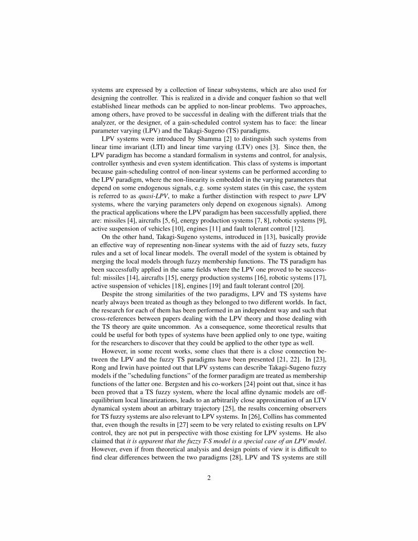
For the models obtained with j = 3 and j = 4, the subsystems in (70) are definedby the following state matrices (see Fig. 1 for a graphical example of how a non-linearsystem equation is described by the subsystems):
A(3)1 =
4 1 0kπ 0 01 1 −1
A(3)2 =
4 −1 0kπ 0 01 1 −1
A(3)3 =
4 1 0−kπ 0 01 1 −1
A(3)
4 =
4 −1 0−kπ 0 01 1 −1
A(3)5 =
1 1 0kπ 0 01 1 −1
A(3)6 =
1 −1 0kπ 0 01 1 −1
A(3)
7 =
1 1 0−kπ 0 01 1 −1
A(3)8 =
1 −1 0−kπ 0 01 1 −1
A(4)1 =
4 1 0qπ π 01 1 −1
A(4)
2 =
4 1 0qπ −π 01 1 −1
A(4)3 =
4 1 0−qπ π 0
1 1 −1
A(4)4 =
4 1 0−qπ −π 0
1 1 −1
A(4)
5 =
4 −1 0qπ π 01 1 −1
A(4)6 =
4 −1 0qπ −π 01 1 −1
A(4)7 =
4 −1 0−qπ π 0
1 1 −1
A(4)
8 =
4 −1 0−qπ −π 0
1 1 −1
A(4)9 =
1 1 0qπ π 01 1 −1
A(4)10 =
1 1 0qπ −π 01 1 −1
A(4)
11 =
1 1 0−qπ π 0
1 1 −1
A(4)12 =
1 1 0−qπ −π 0
1 1 −1
A(4)13 =
1 −1 0qπ π 01 1 −1
A(4)
14 =
1 −1 0qπ −π 01 1 −1
A(4)15 =
1 −1 0−qπ π 0
1 1 −1
A(4)16 =
1 −1 0−qπ −π 0
1 1 −1
where kπ and qπ are constants defined as:
kπ = π√
1 + π2 + π qπ = π√
1 + π2
16
The membership functions M(3)i11, M(3)
i12, M(3)i21, M(4)
i11, M(4)i12, M(4)
i21, M(4)i22 are defined
using (40):
M(3)i11
(ϑ(3)
11 (x1))
=
{sin x1/x1 i = 1, 2, 3, 41 − sin x1/x1 i = 5, 6, 7, 8 (80)
M(3)i12
(ϑ(3)
12 (x2))
=
{1 − sin x2/x2 i = 1, 3, 5, 7sin x2/x2 i = 2, 4, 6, 8 (81)
M(3)i21
(ϑ(3)
21 (x1, x2))
=
x1
√1+x2
2+x2+kπ2kπ
i = 1, 2, 5, 6kπ−x1
√1+x2
2−x2
2kπi = 3, 4, 7, 8
(82)
M(4)i11
(ϑ(4)
11 (x1))
=
{sin x1/x1 i = 1, 2, 3, 4, 5, 6, 7, 81 − sin x1/x1 i = 9, 10, 11, 12, 13, 14, 15, 16 (83)
M(4)i12
(ϑ(4)
12 (x2))
=
{1 − sin x2/x2 i = 1, 2, 3, 4, 9, 10, 11, 12sin x2/x2 i = 5, 6, 7, 8, 13, 14, 15, 16 (84)
M(4)i21
(ϑ(4)
21 (x1, x2))
=
x1
√1+x2
2+qπ2qπ
i = 1, 2, 5, 6, 9, 10, 13, 14qπ−x1
√1+x2
22qπ
i = 3, 4, 7, 8, 11, 12, 15, 16(85)
M(4)i22
(ϑ(4)
22 (x1))
=
{ x1+π2π i = 1, 3, 5, 7, 9, 11, 13, 15π−x1
2π i = 2, 4, 6, 8, 10, 12, 14, 16 (86)
Finally, the coefficients that describe the level of activation of each local model areobtained using (10) as:
ρ(3)i (x1, x2) =
M(3)i11M(3)
i12M(3)i21
8∑i=1
M(3)i11M(3)
i12M(3)i21
(87)
ρ(4)i (x1, x2) =
M(4)i11M(4)
i12M(4)i21M(4)
i2216∑i=1
M(4)i11M(4)
i12M(4)i21M(4)
i22
(88)
Remark 3: Notice that the obtained TS models can be interpreted as if they were LPVsystems as follows: x1
x2x3
= A3 (x1, x2)
x1x2x3
+
1 00 10 0
(
u1u2
)(89)
x1x2x3
= A4 (x1, x2)
x1x2x3
+
1 00 10 0
(
u1u2
)(90)
17
where:
A3 (x1, x2) =
ϑ(3)11 (x1) ϑ(3)
12 (x2) 0ϑ(3)
21 (x1, x2) 0 01 1 −1
=
8∑i=1
ρ(3)i (x1, x2)A(3)
i (91)
A4 (x1, x2) =
ϑ(4)11 (x1) ϑ(4)
12 (x2) 0ϑ(4)
21 (x1, x2) ϑ(4)22 (x1) 0
1 1 −1
=
16∑i=1
ρ(4)i (x1, x2)A(4)
i (92)
where ρ(3)i (x1, x2) and ρ(4)
i (x1, x2) can be interpreted as coefficients of a polytopic de-composition.
−4−2
02
4 −4−2
02
4−20
−15
−10
−5
0
5
10
15
20
x2x
1
dx1/d
t(x 1,x
2)
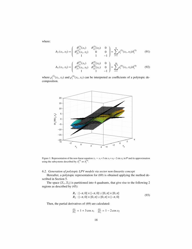
Figure 1: Representation of the non-linear equation x1 = x1+3 sin x1+x2−2 sin x2 inP and its approximationusing the subsystems described by A(3)
i or A(4)i .
6.2. Generation of polytopic LPV models via sector non-linearity conceptHereafter, a polytopic representation for (69) is obtained applying the method de-
scribed in Section 5.The space {X1,X2} is partitioned into 4 quadrants, that give rise to the following 2
regions as described by (45):
R1 : [−π, 0] × [−π, 0] ∪ [0, π] × [0, π]R2 : [−π, 0] × [0, π] ∪ [0, π] × [−π, 0] (93)
Then, the partial derivatives of (69) are calculated:
∂ f1∂x1
= 1 + 3 cos x1∂ f1∂x2
= 1 − 2 cos x2
18
∂ f2∂x1
= 2x1
√1 + x2
2 + x2∂ f2∂x2
=x2
1 x2√1+x2
2
+ x1
and their minimum and maximum values in R1 and R2 are found:
a(1)11 = max
R1
∂ f1∂x1
= 4 a(1)11 = min
R1
∂ f1∂x1
= −2
a(2)11 = max
R2
∂ f1∂x1
= 4 a(2)11 = min
R2
∂ f1∂x1
= −2
a(1)12 = max
R1
∂ f1∂x2
= 3 a(1)12 = min
R1
∂ f1∂x2
= −1
a(2)12 = max
R2
∂ f1∂x2
= 3 a(2)12 = min
R2
∂ f1∂x2
= −1
a(1)21 = max
R1
∂ f2∂x1
= rπ + π a(1)21 = min
R1
∂ f2∂x1
= − (rπ + π)
a(2)21 = max
R2
∂ f2∂x1
= rπ − π a(2)21 = min
R2
∂ f2∂x1
= −rπ + π
a(1)22 = max
R1
∂ f2∂x2
= wπ + π a(1)22 = min
R1
∂ f2∂x2
= − (wπ + π)
a(2)22 = max
R2
∂ f2∂x2
= wπ − π a(2)22 = min
R2
∂ f2∂x2
= −wπ + π
where:rπ = 2π
√1 + π2 wπ = π3
√1+π2
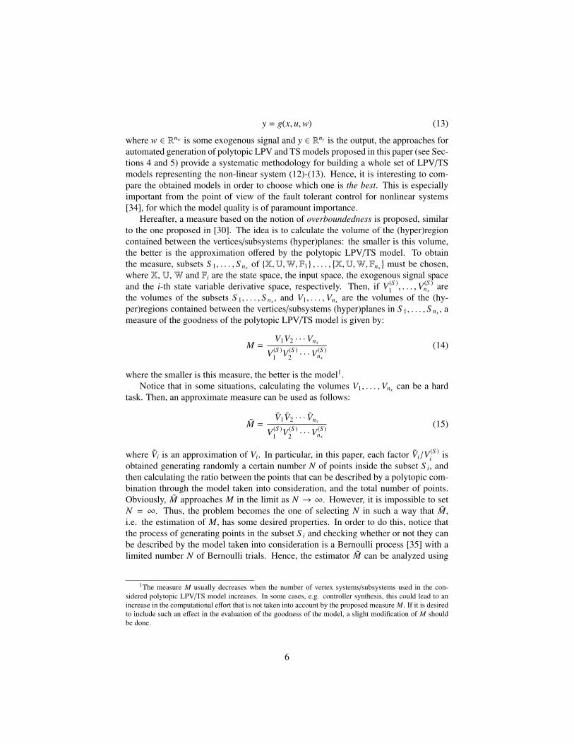
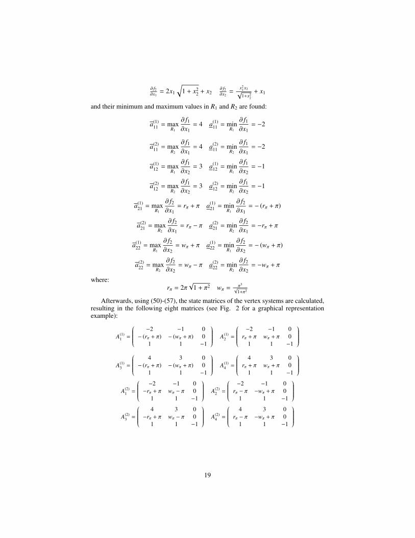
Afterwards, using (50)-(57), the state matrices of the vertex systems are calculated,resulting in the following eight matrices (see Fig. 2 for a graphical representationexample):
A(1)1 =
−2 −1 0− (rπ + π) − (wπ + π) 0
1 1 −1
A(1)2 =
−2 −1 0rπ + π wπ + π 0
1 1 −1
A(1)
3 =
4 3 0− (rπ + π) − (wπ + π) 0
1 1 −1
A(1)4 =
4 3 0rπ + π wπ + π 0
1 1 −1
A(2)
1 =
−2 −1 0−rπ + π wπ − π 0
1 1 −1
A(2)2 =
−2 −1 0rπ − π −wπ + π 0
1 1 −1
A(2)
3 =
4 3 0−rπ + π wπ − π 0
1 1 −1
A(2)4 =
4 3 0rπ − π −wπ + π 0
1 1 −1
19

such that (69) results expressed in the following polytopic LPV form: x1x2x3
=
4∑j=1
α(1)j (x1, x2)A(1)
j
x1x2x3
+
4∑j=1
α(2)j (x1, x2)A(2)
j
x1x2x3
+
1 00 10 0
(
u1u2
)(94)
where the coefficients of the polytopic decomposition are obtained using (59)-(61), asfollows:
α(1)1 (x1, x2) =
_α
(1)1 (x1, x2)_α
(1)2 (x1, x2)R∈1(x1, x2)
α(1)2 (x1, x2) =
_α
(1)1 (x1, x2)^α
(1)2 (x1, x2)R∈1(x1, x2)
α(1)3 (x1, x2) =
^α
(1)1 (x1, x2)_α
(1)2 (x1, x2)R∈1(x1, x2)
α(1)4 (x1, x2) =
^α
(1)1 (x1, x2)^α
(1)2 (x1, x2)R∈1(x1, x2)
α(2)1 (x1, x2) =
_α
(2)1 (x1, x2)_α
(2)2 (x1, x2)R∈2(x1, x2)
α(2)2 (x1, x2) =
_α
(2)1 (x1, x2)^α
(2)2 (x1, x2)R∈2(x1, x2)
α(2)3 (x1, x2) =
^α
(2)1 (x1, x2)_α
(2)2 (x1, x2)R∈2(x1, x2)
α(2)4 (x1, x2) =
^α
(2)1 (x1, x2)^α
(2)2 (x1, x2)R∈2(x1, x2)
with:_α
(1)1 (x1, x2) =
3x1 + 2x2 − 3 sin x1 + 2 sin x2
6x1 + 4x2
^α
(1)1 (x1, x2) =
3x1 + 2x2 + 3 sin x1 − 2 sin x2
6x1 + 4x2
_α
(2)1 (x1, x2) =
3x1 − 2x2 − 3 sin x1 + 2 sin x2
6x1 − 4x2
^α
(2)1 (x1, x2) =
3x1 − 2x2 + 3 sin x1 − 2 sin x2
6x1 − 4x2
_α
(1)2 (x1, x2) =
(rπ + π) x1 + (wπ + π) x2 − x21
√1 + x2
2 − x1x2
2 [(rπ + π) x1 + (wπ + π) x2]
^α
(1)2 (x1, x2) =
(rπ + π) x1 + (wπ + π) x2 + x21
√1 + x2
2 + x1x2
2 [(rπ + π) x1 + (wπ + π) x2]
_α
(2)2 (x1, x2) =
(rπ − π)x1 + (π − wπ)x2 − x21
√1 + x2
2 − x1x2
2 [(rπ − π)x1 + (π − wπ)x2]
^α
(2)2 (x1, x2) =
(rπ − π)x1 + (π − wπ)x2 + x21
√1 + x2
2 + x1x2
2 [(rπ − π)x1 + (π − wπ)x2]
20
R∈1(x1, x2) = max (0, sgn(x1)sgn(x2))
R∈2(x1, x2) = max (0,−sgn(x1)sgn(x2))
where sgn denotes the sign function.Remark 4: Notice that the quasi-LPV representation of (69) obtained using this
method has the following structure: x1x2x3
=
a11(x1, x2) a12(x1, x2) 0a21(x1, x2) a22(x1, x2) 0
1 1 −1
x1
x2x3
+
1 00 10 0
(
u1u2
)(95)
Remark 5: The obtained quasi-LPV system can be interpreted as a Takagi-Sugenomodel, if a11(x1, x2), a12(x1, x2), a21(x1, x2), a22(x1, x2) in (95) and sgn(x1)sgn(x2) areconsidered to be the premise variables, and _
α(1)1 , ^
α(1)1 , _
α(2)1 , ^
α(2)1 , _
α(1)2 , ^
α(1)2 , _
α(2)2 , ^
α(2)2 , R∈1 ,
R∈2 the membership functions.
−4 −2 0 2 4 −4 −2 0 2 4−25
−20
−15
−10
−5
0
5
10
15
20
25
x2x
1
dx1/d
t(x 1,x
2)
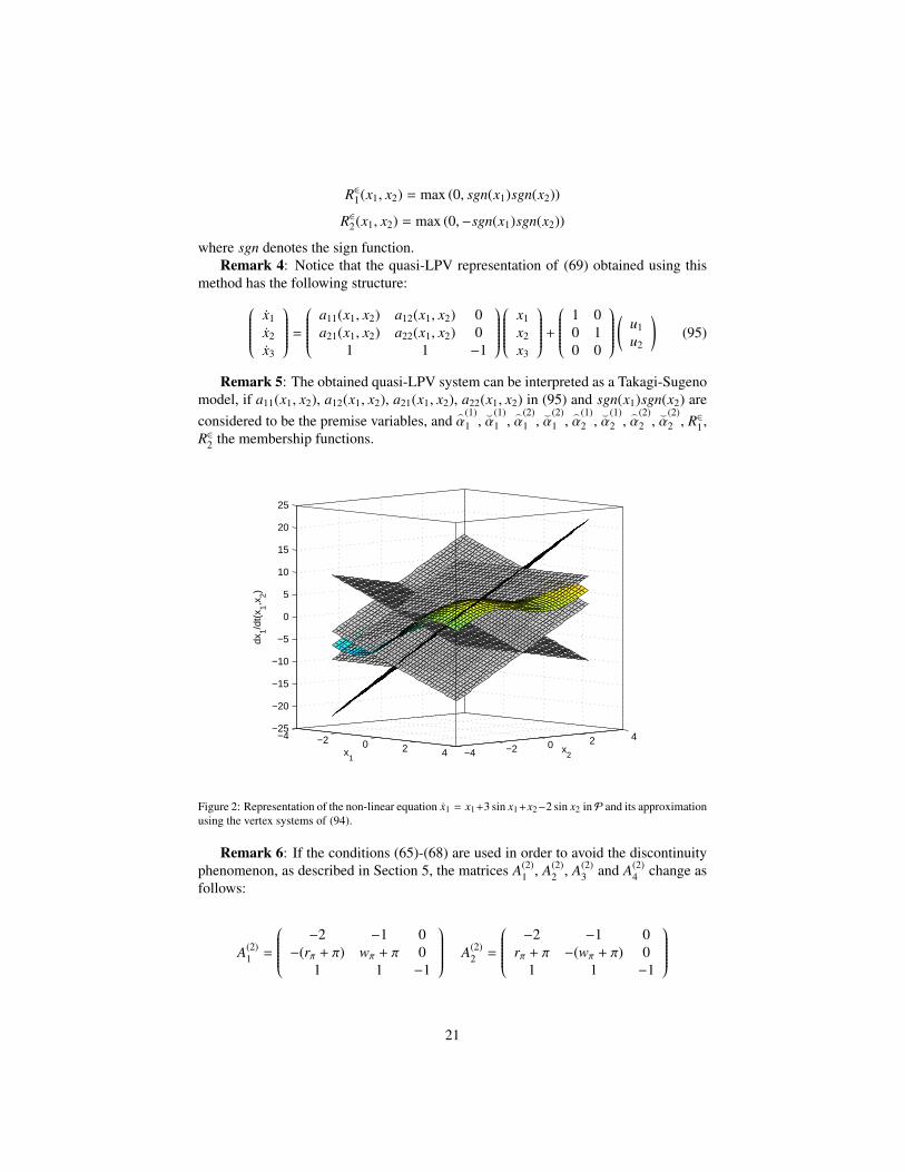
Figure 2: Representation of the non-linear equation x1 = x1+3 sin x1+x2−2 sin x2 inP and its approximationusing the vertex systems of (94).
Remark 6: If the conditions (65)-(68) are used in order to avoid the discontinuityphenomenon, as described in Section 5, the matrices A(2)
1 , A(2)2 , A(2)
3 and A(2)4 change as
follows:
A(2)1 =
−2 −1 0−(rπ + π) wπ + π 0
1 1 −1
A(2)2 =
−2 −1 0rπ + π −(wπ + π) 0
1 1 −1
21

A(2)3 =
4 3 0−(rπ + π) wπ + π 0
1 1 −1
A(2)4 =
4 3 0rπ + π −(wπ + π) 0
1 1 −1
6.3. Comparison
Hereafter, the comparison criteria between models described in Section 3 are ap-plied to the proposed example.
The subsets S 1 ⊂ X1 × X2 × X1 and S 2 ⊂ X1 × X2 × X2 are chosen as follows:
S 1 = [−π, π] × [−π, π] × [−7π, 7π] (96)
S 2 = [−π, π] × [−π, π] × [−hπ, hπ] (97)
with:
hπ = π2(2 + 2
√1 + π2 +
π2
√1 + π2
)so that:
V (S )1 = 56π3 V (S )
2 = 8π2hπ
The volumes Vi have been calculated using (15) on the basis of N = 16588 points4,generated randomly using a uniform distribution:
Model generated via non-linear embedding A(3)i :
V1
V (S )1
=5856 + 3.317916588 + 6.6358
= 0.35V2
V (S )2
=6178 + 3.3179
16588 + 6.6358= 0.37 M =
V1V2
V (S )1 V (S )
2
= 0.13
Model generated via non-linear embedding A(4)i :
V1
V (S )1
=5856 + 3.317916588 + 6.6358
= 0.35V2
V (S )2
=4866 + 3.3179
16588 + 6.6358= 0.29 M =
V1V2
V (S )1 V (S )
2
= 0.10
Model generated via sector non-linearity concept:
V1
V (S )1
=7546 + 3.317916588 + 6.6358
= 0.45V2
V (S )2
=9844 + 3.3179
16588 + 6.6358= 0.59 M =
V1V2
V (S )1 V (S )
2
= 0.27
Model generated via sector non-linearity concept (conservative):
V1
V (S )1
=7546 + 3.317916588 + 6.6358
= 0.45V2
V (S )2
=11197 + 3.317916588 + 6.6358
= 0.67 M =V1V2
V (S )1 V (S )
2
= 0.30
4This particular value of N is chosen using statistical reasoning, in order to guarantee that the semi-length of the 99% Agresti-Coull confidence interval will be less than 0.01 [51].
22
Hence, according to the measure of overboundedness (15), the best model is theone generated via non-linear embedding and described by the matrices A(4)
i . In general,models obtained via non-linear embedding tend to be less conservative than the onesobtained via sector non-linearity concept. This is probably due to the fact that the non-linear embedding method tries to find the maximum and minimum value of f (x)/xi,whereas the other method finds the maximum and minimum value of ∂ f (x)/∂xi. Then,according to the mean-value theorem, f (x)/xi is bounded by ∂ f (x)/∂xi, so that theextreme values of the former are smaller than those of the latter.
To conclude the comparison between the models, let us consider the measure basedon the region of attraction as introduced in Section 3.2, with controllers designed ap-plying Theorem 2 to the following LMI region:
D = {z ∈ C : Re(z) < −1} (98)
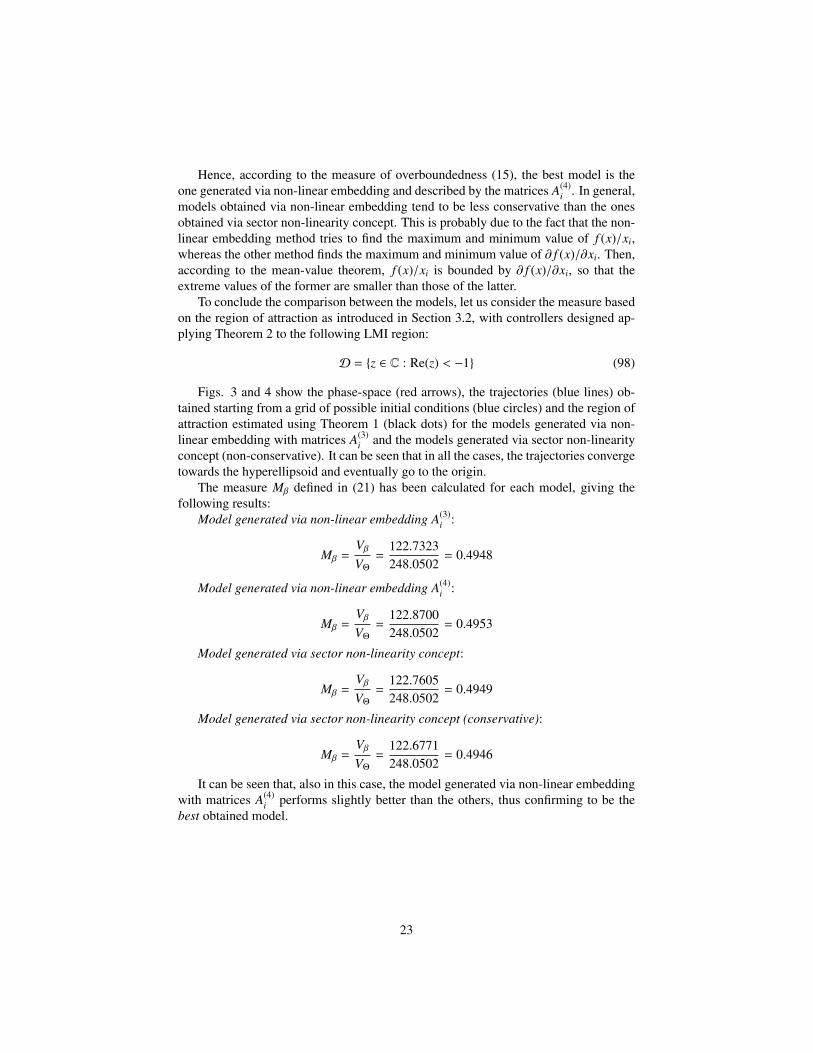
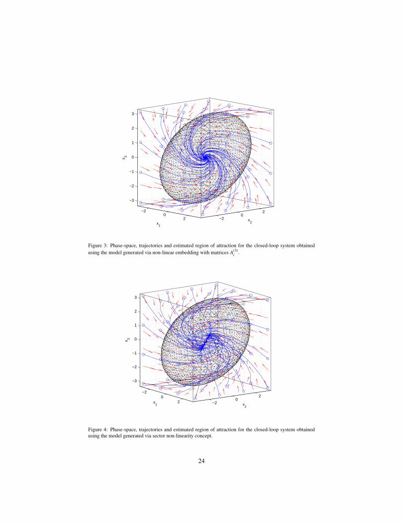
Figs. 3 and 4 show the phase-space (red arrows), the trajectories (blue lines) ob-tained starting from a grid of possible initial conditions (blue circles) and the region ofattraction estimated using Theorem 1 (black dots) for the models generated via non-linear embedding with matrices A(3)
i and the models generated via sector non-linearityconcept (non-conservative). It can be seen that in all the cases, the trajectories convergetowards the hyperellipsoid and eventually go to the origin.
The measure Mβ defined in (21) has been calculated for each model, giving thefollowing results:
Model generated via non-linear embedding A(3)i :
Mβ =Vβ
VΘ
=122.7323248.0502
= 0.4948
Model generated via non-linear embedding A(4)i :
Mβ =Vβ
VΘ
=122.8700248.0502
= 0.4953
Model generated via sector non-linearity concept:
Mβ =Vβ
VΘ
=122.7605248.0502
= 0.4949
Model generated via sector non-linearity concept (conservative):
Mβ =Vβ
VΘ
=122.6771248.0502
= 0.4946
It can be seen that, also in this case, the model generated via non-linear embeddingwith matrices A(4)
i performs slightly better than the others, thus confirming to be thebest obtained model.
23
−20
2 −20
2
−3
−2
−1
0
1
2
3
x2x
1
x 3
Figure 3: Phase-space, trajectories and estimated region of attraction for the closed-loop system obtainedusing the model generated via non-linear embedding with matrices A(3)
i .
−20
2 −20
2
−3
−2
−1
0
1
2
3
x2
x1
x 3
Figure 4: Phase-space, trajectories and estimated region of attraction for the closed-loop system obtainedusing the model generated via sector non-linearity concept.
24
7. Conclusions
In this paper, the presence of strong analogies between polytopic LPV and TSsystems and the automated generation of polytopic LPV and TS models have beenaddressed. In particular, it has been shown that the method for the automated gen-eration of LPV models by non-linear embedding can be easily extended to generateautomatically TS models from a given non-linear system. Analogously, a method al-ready used in the TS framework for finding a model that describes in a fuzzy way agiven non-linear function has been extended to the case of polytopic LPV descriptionof non-linear systems.
Results obtained with a mathematical example have been presented and it has beenshown, using an overboundedness measure, that the automatic generation via non-linear embedding provides less conservative models than the automated generation viasector non-linearity concept. Also, a measure based on the region of attraction esti-mates has been introduced for comparing the closed-loop performances of the differentmodels.
The overboundedness measure has shown to be an objective criterion that can beused to select which model can be considered the best. However, in the general case,which model is the best also depends on the context in which the model is used,i.e. whether it is used for stabilization or observation, and which structure of con-troller/observer is used for achieving the desired goal. Some information in this sensehas been provided by the measure based on the region of attraction estimates, that al-lows comparing the closed-loop performances obtained with the different models whenconsidering a quadraticD-stabilizing state-feedback controller in the design step. Theproposed measure could be easily extended to other controller structures, e.g. output-feedback controllers, and to the observation case. However, it has the limit of providingan indication of which model is the best only a posteriori. It seems clear that an im-portant path for future research is the development of a procedure that automaticallyselects the best model during the design step, taking into account what the model isused for and the used controller/observer structure.
Acknowledgment
This work has been funded by the Spanish Ministry of Science and Technologythrough the projects CICYT SHERECS (ref. DPI2011-26243) and CICYT ECO-CIS (ref. DPI2013-48243-C2-1-R), by the European Commission through contracti-Sense FP7-ICT-2009-6-270428, by UPC through the grant FPI-UPC E-01104, byAGAUR through the contracts FI-DGR 2013 (ref. 2013FIB00218) and FI-DGR 2014(ref. 2014FI B1 00172), and by the DGR of Generalitat de Catalunya (SAC groupRef. 2014/SGR/374). The work was also supported by the National Science Centre inPoland under the grant 2013/11/B/ST7/01110.
25

References
References
[1] D. J. Leith, W. E. Leithead, Survey of gain-scheduling analysis design, Interna-tional Journal of Control 73 (2000) 1001–1025.
[2] J. S. Shamma, Analysis and design of gain scheduled control systems, Ph.D. the-sis, Massachussets Institute of Technology, Department of Mechanical Engineer-ing, advised by M. Athans, 1988.
[3] J. S. Shamma, An overview of LPV systems, in: J. Mohammadpour, C. Scherer(Eds.), Control of linear parameter varying systems with applications, Springer,2012, pp. 3–26.
[4] P. C. Pellanda, P. Apkarian, H. D. Tuan, Missile autopilot design via a multi-channel LFT/LPV control method, International Journal of Robust and NonlinearControl 12 (2002) 1–20.
[5] V. Verdult, M. Lovera, M. Verhaegen, Identification of linear parameter varyingstate space models with application to helicopter rotor dynamics, InternationalJournal of Control 77 (2004) 1149–1159.
[6] D. Rotondo, F. Nejjari, V. Puig, Quasi-LPV modeling, identification and controlof a twin rotor MIMO system, Control Engineering Practice 21 (2013) 829–846.
[7] G. J. Balas, Linear parameter-varying control and its application to a turbofanengine, International Journal of Robust and Nonlinear Control 12 (2002) 763–796.
[8] F. D. Bianchi, R. J. Mantz, C. F. Christiansen, Gain scheduling control of variable-speed wind energy conversion systems using quasi-LPV models, Control Engi-neering Practice 13 (2005) 247–255.
[9] Z. Yu, H. Chen, P. Woo, Gain scheduled LPV H∞ control based on LMI approachfor a robotic manipulator, Journal of Robotic Systems 19 (2002) 585–593.
[10] P. Gaspar, I. Szaszi, J. Bokor, Active suspension design using linear parametervarying control, International Journal of Vehicle Autonomous Systems 1 (2003)206–221.
[11] B. Boulkroune, I. Djemili, A. Aitouche, V. Cocquempot, Robust nonlinear ob-server design for actuator fault detection in diesel engines, International Journalof Applied Mathematics and Computer Science 23 (2013) 557–569.
[12] S. Montes De Oca, V. Puig, M. Witczak, L. Dziekan, Fault-tolerant control strat-egy for actuator faults using lpv techniques: application to a two degree of free-dom helicopter, International Journal of Applied Mathematics and ComputerScience 22 (2012) 161–171.
26

[13] T. Takagi, M. Sugeno, Fuzzy identification of systems and its applications tomodeling and control, IEEE Transactions on Systems, Man, and CyberneticsSMC-15 (1985) 116–132.
[14] X.-H. Yuan, J.-C. Ren, Y.-J. He, F.-C. Sun, Synthesis of H2 guaranteed costfuzzy controller for missile altitude system via linear matrix inequalities, in:Proceedings of the 2004 American Control Conference, volume 3, pp. 2309–2313.
[15] Ł. Dziekan and M. Witczak and J. Korbicz, Active fault-tolerant control designfor Takagi-Sugeno fuzzy systems, Bulletin of the Polish Academy of Sciences,Technical Sciences 59 (2011) 93–102.
[16] H.-S. Ko and K. Jatskevich, Power quality control of wind-hybrid power gener-ation system using fuzzy-LQR controller, IEEE Transactions on Energy Conver-sion 22 (2007) 516–527.
[17] O. Begovich and E. N. Sanchez and M. Maldonado, Takagi-Sugeno fuzzy schemefor real-time trajectory tracking of an underactuated robot, IEEE Transactions onControl Systems Technology 10 (2002) 14–20.
[18] J. Cao and P. Li and H. Liu, An interval fuzzy controller for vehicle active suspen-sion systems, IEEE Transactions on Intelligent Transportation Systems 11 (2010)885–895.
[19] D. Khiar and J. Lauber and T. Floquet and G. Colin and T. M. Guerra and Y.Chamaillard, Robust Takagi-Sugeno fuzzy control of a spark ignition engine,Control Engineering Practice 15 (2007) 1446–1456.
[20] D. Ichalal and B. Marx and J. Ragot and D. Maquin, New fault tolerant controlstrategies for nonlinear Takagi-Sugeno systems, International Journal of AppliedMathematics and Computer Science 22 (2012) 197–210.
[21] P. M. Makila, P. Viljamaa, Convex parametric design, gain scheduling, and fuzzycomputing, Technical Report, Tampere, Tampere University of Technology, In-stitute of Automation and Control, 2002.
[22] P. M. Makila, P. Viljamaa, Linear programming based gain scheduling for LPVand PL systems, in: Proceedings of the 15th IFAC World Congress (2002).
[23] Q. Rong, G. W. Irwin, LMI-based control design for discrete polytopic LPVsystems, in: Proceedings of the 6th European Control Conference (2003).
[24] P. Bergsten, R. Palm, D. Driankov, Observers for Takagi-Sugeno fuzzy systems,IEEE Transactions on Systems, Man, and Cybernetics - Part B: Cybernetics 32(2002) 114–121.
[25] T. A. Johansen, R. Shorten, R. M. Smith, On the interpretation and identifica-tion of dynamic Takagi-Sugeno models, IEEE Transactions on Fuzzy Systems 8(2000) 297–313.
27

[26] E. G. Collins, Book Review: Fuzzy control systems design and analysis: a linearmatrix inequality approach, Automatica 39 (2003) 2011–2019.
[27] K. Tanaka, H. O. Wang, Fuzzy control systems design and analysis: A linearmatrix inequality approach, John Wiley and Sons, Inc., 2001.
[28] K. Tanaka, H. Ohtake, H. O. Wang, Recursive pointwise design for nonlinearsystems, in: Proceedings of the 2004 American Control Conference, volume 1,pp. 470–475.
[29] R. Toth, Modeling and identification of linear parameter-varying systems,Springer, 2010.
[30] A. Kwiatkowski, M.-T. Boll, H. Werner, Automated generation and assessmentof affine LPV models, in: Proceedings of the 45th IEEE Conference on Decisionand Control, San Diego, CA, USA (2006), pp. 6690–6695.
[31] H. Ohtake, K. Tanaka, H. O. Wang, Fuzzy modeling via sector nonlinearity con-cept, Integrated Computer-Aided Engineering 10 (2003) 333–341.
[32] P. Apkarian, P. Gahinet, G. Becker, Self-scheduled H∞ control of linearparameter-varying systems: A design example, Automatica 31 (1995) 1251 –1261.
[33] J. S. Shamma, J. R. Cloutier, Gain-scheduled missile autopilot design using linearparameter varying transformations, Journal of Guidance, Control, and Dynamics16 (1993) 256–263.
[34] M. Witczak, V. Puig, S. Montes De Oca, A fault-tolerant control strategy for non-linear discrete-time systems: application to the twin-rotor system, InternationalJournal of Control 86 (2013) 1788–1799.
[35] J. Bernoulli, Ars conjectandi, opus posthumum. Accedit Tractatus de seriebusinfinitis, et epistola gallice scripta de ludo pilae reticularis, Basel: ThurneysenBrothers, 1713.
[36] D. C. Montgomery, G. C. Runger, Applied statistics and probability for engineers,Wiley-Interscience, 1999.
[37] P. Apkarian, P. Gahinet, A convex characterization of gain-scheduled H∞ con-trollers, IEEE Transactions on Automatic Control 40 (1995) 853–864.
[38] P. Gahinet, P. Apkarian, M. Chilali, Affine parameter-dependent Lyapunov func-tions and real parametric uncertainty, IEEE Transactions on Automatic Control41 (1996) 436–442.
[39] F. Bruzelius, S. Pettersson, C. Breitholtz, Region of attraction estimates for LPV-gain scheduled control systems, in: Proceedings of the 7th European ControlConference.
[40] H. Khalil, Nonlinear systems, Prentice-Hall, Inc, Upper Saddle River, 1996.
28

[41] G. Becker, A. Packard, Robust performance of linear parametrically varyingsystems using parametrically-dependent linear feedback, Systems and ControlLetters 23 (1994) 205–215.
[42] M. Chilali, P. Gahinet, H∞ design with pole placement constraints: An LMIapproach, IEEE Transactions on Automatic Control 41 (1996) 358–367.
[43] B. A. Francis, A course in H∞ Control Theory, Lecture Notes in Control andInformation Sciences, no. 88. Berlin: Springer-Verlag, 1987.
[44] S. Gutman, E. I. Jury, A general theory for matrix root clustering in subregionsof the complex plane, IEEE Transactions on Automatic Control AC-26 (1981)853–863.
[45] A. S. Ghersin, R. S. Sanchez-Pena, LPV control of a 6 DOF vehicle, IEEETransactions on Control Systems Technology 10 (2002) 883–887.
[46] D. Rotondo, F. Nejjari, V. Puig, A virtual actuator and sensor approach for faulttolerant control of LPV systems, Journal of Process Control 24 (2014) 203–222.
[47] T. M. Guerra, A. Kruszewski, J. Lauber, Discrete Tagaki–Sugeno models forcontrol: Where are we?, Annual Reviews in control 33 (2009) 37–47.
[48] R. A. Horn, C. R. Johnson, Matrix analysis, Cambridge University Press, 1990.
[49] X.-D. Sun, I. Postlethwaite, Affine LPV modelling and its use in gain-scheduledhelicopter control, in: UKACC International Conference on Control (1998), vol-ume 2, pp. 1504–1509.
[50] S. Kawamoto, K. Tada, A. Ishigame, T. Taniguchi, An approach to stabilityanalysis of second order fuzzy systems, in: Proceedings of the InternationalConference on Fuzzy Systems (1992), pp. 1427–1434.
[51] A. Agresti and B. A. Coull, Approximate is better than exact for interval estima-tion of binomial proportions, The American Statistician 52 (1998) 119–126.
29