Fuzzy model-based predictive control using Takagi–Sugeno ...bme2.aut.ac.ir/~towhidkhah/MPC/seminars-ppt/89/FUZZYMPC-Chares… · Takagi–Sugeno fuzzy models are suitable to model

Fuzzy model-based predictive control usingTakagi±Sugeno models

J.A. Roubos *, S. Mollov, R. Babu�ska, H.B. Verbruggen

Faculty of Information Technology and Systems, Delft University of Technology, Control

Laboratory, P.O. Box 5031, 2600 GA Delft, The Netherlands

Received 01 October 1998; accepted 01 February 1999

Abstract

Nonlinear model-based predictive control (MBPC) in multi-input multi-output

(MIMO) process control is attractive for industry. However, two main problems

need to be considered: (i) obtaining a good nonlinear model of the process, and

(ii) applying the model for control purposes. In this paper, recent work focusing on the

use of Takagi±Sugeno fuzzy models in combination with MBPC is described. First, the

fuzzy model-identi®cation of MIMO processes is given. The process model is derived

from input±output data by means of product-space fuzzy clustering. The MIMO model

is represented as a set of coupled multi-input, single-output (MISO) models. Next, the

Takagi±Sugeno fuzzy model is used in combination with MBPC. The critical element in

nonlinear MBPC is the optimization routine which is nonconvex and thus di�cult to

solve. Two methods to deal with this problem are developed: (i) a branch-and-bound

method with iterative grid-size reduction, and (ii) control based on a local linear model.

Both methods have been tested and evaluated with a simulated laboratory setup for a

MIMO liquid level process with two inputs and four outputs. Ó 1999 Elsevier Science

Inc. All rights reserved.

Keywords: Model-based predictive control (MBPC); Nonlinear control; MIMO

systems; Takagi±Sugeno fuzzy model

International Journal of Approximate Reasoning 22 (1999) 3±30

*Corresponding author. Tel.: +31-15-278-3371; fax: +31-15-278-6679; e-mail:

[email protected]

0888-613X/99/$ - see front matter Ó 1999 Elsevier Science Inc. All rights reserved.

PII: S 0 8 8 8 - 6 1 3 X ( 9 9 ) 0 0 0 2 0 - 1

1. Introduction

Model-based predictive control (MBPC) is a powerful tool for the control ofmultivariable systems. It has become a major research topic during the last fewdecades and, unlike many other advanced techniques, it has also been suc-cessfully applied in industry [1]. The main reason for this success is the abilityof MBPC to control multivariable systems under various constraints in anoptimal way. However, two major issues limit the possible application ofMBPC to nonlinear systems:1. a model must be made that predicts the process variables over the speci®ed

prediction horizon with su�cient accuracy, and2. given a nonlinear process model, a nonlinear (and usually nonconvex) opti-

mization problem must be solved for each sampling period.The ®rst factor hampers the application of MBPC to complex or partially

known systems, for which reliable analytical models cannot be obtained. Thesecond factor hampers the application to fast systems, where iterative opti-mization techniques cannot be used properly, due to short sampling periods. Inthis article we propose using fuzzy MBPC (FMBPC) to deal with both issues.

To avoid confusion, we explain the term FMBPC, because it has been givenseveral di�erent meanings in the literature. First, a fuzzy model can be used asa predictor in MBPC [2±4], second, the constraints or objective functions canbe fuzzy [5], and third, the optimizer, including the control strategy, can bebased on fuzzy rules [6]. In this article, the use of Takagi±Sugeno fuzzy models[7] in MBPC is investigated.

Model-based controllers use an internal model to predict future outputs.These future outputs can be calculated by means of di�erent optimizationmethods, depending on the system and objective functions. Generally, pref-erence is given to optimization problems that can be optimized by means ofconvex optimization methods. Two methods, which combine Takagi±Sugenomodels with MBPC are presented in this article: (i) a branch-and-boundmethod in combination with the nonlinear model, (ii) linear MBPC using eithera single or multiple linear models extracted from the Takagi±Sugeno fuzzymodel. The ®rst method is a standard MISO branch-and-bound algorithm thathas been extended to MIMO systems. Further, a major extension to reduce theassociated computational burden has been made. The second technique com-bines linear MBPC with local linear models that are extracted from theTakagi±Sugeno fuzzy model by a so-called `linearization'. It is not local line-arization around a working point (in the sense of Lyapunov). However, it isalso not `nonlinearity hiding'. The TS model can be seen as a linear model withtime-varying (in fact state-dependent) parameters. Like in certainty-equiva-lence adaptive control, one can `freeze' these parameters and use the current`linear' model in the MBPC optimization. This method is divided into single-step linearization and multi-step linearization, depending on whether the model

4 J.A. Roubos et al. / Internat. J. Approx. Reason. 22 (1999) 3±30

is extracted at the current point or at a sequence of points within the predictionhorizon. The resulting receding horizon controllers are used in the internalmodel control (IMC) scheme to eliminate control errors due to disturbancesand model mismatch.

The paper is organized as follows. Sections 2 and 3 provide the necessarybackground information on the Takagi±Sugeno fuzzy model and on MBPC.The main contribution of the paper is presented in Sections 4 and 5: Section 4describes nonlinear optimization based on the branch-and-bound method, andSection 5 deals with local linearization approaches. Section 6 presents acomplete MBPC scheme including an internal model which is used to elimi-nate control errors due to disturbances. Both developed methods have beentested and evaluated on a simulated laboratory setup. Results and a discussionare given in Section 7. Section 8 draws some conclusion from the presentedwork.

2. Fuzzy modeling

Takagi±Sugeno fuzzy models are suitable to model a large class of nonlinearsystems [8±10]. Fuzzy modeling and identi®cation from measured data aree�ective tools for the approximation of uncertain nonlinear systems. So far,most attention has been devoted to single-input, single-output (SISO) or multi-input, single-output (MISO) systems. Recently, also methods have been pro-posed to deal with multi-input, multi-output (MIMO) systems [11±13]. Mostarticles deal with various aspects of multivariable relational models, such as thedecomposition of fuzzy relations, simpli®cation of the models to avoid memoryoverload, etc. Relatively little attention has been devoted to the identi®cationof MIMO fuzzy models from input±output data. Babu�ska et al. [14] developeda MIMO identi®cation algorithm which uses input±output data. This algo-rithm is used to obtain MIMO Takagi±Sugeno models which can be used forcontrol purposes.

The fuzzy model is structured as follows. Consider a MIMO system with ni

inputs: u 2 U � Rni , and no outputs: y 2 Y � Rno . (Note that we use boldfaceletters to denote vectors and roman letters for matrices.) This system is ap-proximated by a collection of coupled MISO discrete-time fuzzy models. De-note by qÿ1 the backward shift operator: qÿ1y�k� �def y�k ÿ 1�, where y is a signalsampled at discrete time instants k. Denote by f and g polynomials in qÿ1, e.g.,f � a0 � a1qÿ1 � a2qÿ2 � � � �. Given two integers, m6 n, de®ne an ordered se-quence of delayed samples of the signal y as

fy�k�gnm �def�y�kÿm�; y�kÿmÿ 1�; . . . ; y�kÿmÿ n� 1��: �1�

The MISO models are of the input±output NARX type (Nonlinear AutoRegressive model with eXogenous inputs [15])

J.A. Roubos et al. / Internat. J. Approx. Reason. 22 (1999) 3±30 5

yl�k � 1� �Fl xl�k�� ; l � 1; 2; . . . ; no; �2�

where the regression vector xl�k� is given by

xl�k� �hfy1�k�gnyl1

0 ; . . . ; fyno�k�gnylno0 ;

fu1�k � 1�gnul1

ndl1; . . . ; funi�k � 1�gnulni

ndlni

i: �3�

Here ny and nu are matrices with the number of delays in each output andinput, respectively, and nd is the matrix with the numbers of pure (transport)delays from each input to the output. ny is an no � no matrix, and nu; nd areno � ni matrices. Fl are rule-based fuzzy models of the Takagi±Sugeno type [7].With the antecendent in the conjunctive form, the rules are

Rli : If xl1�k� is Xli1 and . . . and xlp�k� is Xlip

then yli�k � 1� � fliy�k� � gliu�k� � hli

i � 1; 2; . . . ;Kl: �4�Here xli is an element from the regression vector (Eq. 3), Xli is the ante-

cedent fuzzy set of the ith rule, f and g are vectors of polynomials and h is theo�set vector. Kl is the number of rules in the lth model. The fuzzy sets X can bede®ned by multivariate membership functions x�x�k�� : Rpl ! �0; 1�, wherepl �

Pnoj�1 nylj �

Pnij�1 nulj is the dimension of the antecedent space [8]. The

MIMO Takagi±Sugeno rules are estimated from input±output system data. AGustafson±Kessel clustering algorithm is used to obtain multivariatemembership functions. Thereafter Takagi±Sugeno rules are derived with aleast-squares algorithm. A description of the used method and the MATLABATLAB

software for automatic MIMO Takagi±Sugeno model extraction is givenin [14].

The choice of the right NARX structure is very important. One can usephysical knowledge to choose a proper structure (see Section 6). Anothermethod is a search through a (large) set of possible structures. The quality ofthe model depends to a great extent on the information content of the input±output data set. It is di�cult to design a good identi®cation signal, especiallyfor MIMO systems. Filtered random signals with additional white noise seemto be appropriate. These signals walk slowly through the whole control domainand continuously excite the system.

The performance of the obtained models is measured by the variance ac-counted for (VAF) index given by

VAF � 100% 1

�ÿ var�Y ÿ Ym�

var�Y ��; �5�

where Y is the true output and Ym is the simulated model output.


3. Basic elements of model based predictive control

MBPC is a general methodology for solving control problems in the timedomain. It is based on three main concepts [16]:1. Explicit use of a model to predict the process output.2. Computation of a sequence of future control actions by minimizing a given

objective function.3. The use of the receding horizon strategy: only the ®rst control action in the

sequence is applied, the horizons are moved one sample period towards thefuture, and optimization is repeated.Because of the optimization approach and the explicit use of the process

model, MBPC can realize multivariable optimal control, deal with nonlinearprocesses and handle constraints e�ciently. The three basic elements ofMBPC: (i) a model which describes the process, (ii) a goal, de®ned by an ob-jective function and constraints (optional), and (iii) an optimization procedure,are described in more detail in the sequal.

3.1. Process model

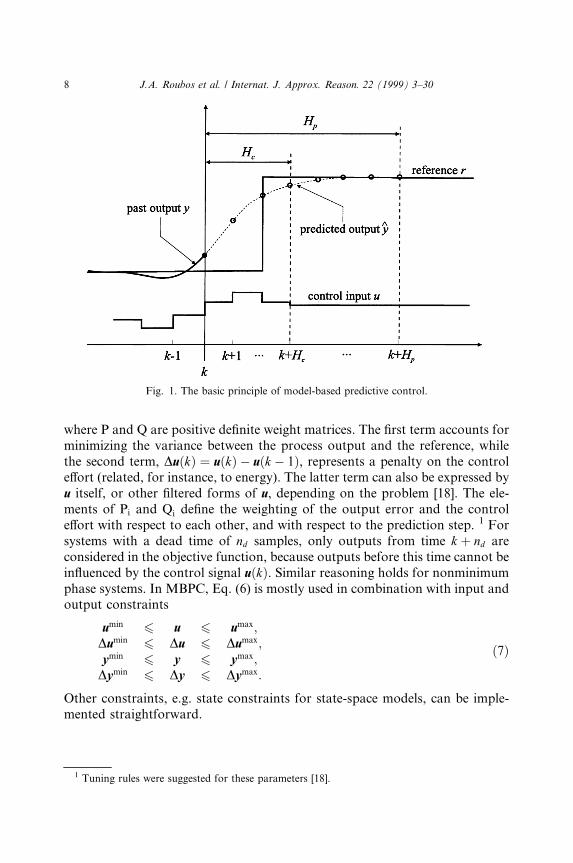
The model must describe the system well and it does not matter what type ofmodel is used to this end: a black-box, a gray-box, or a white-box one [17]. Thefuture process outputs y�k � i� for i � 1; . . . ;Hp, are predicted over the pre-diction horizon Hp using a model of the process. These values depend on thecurrent process state, and on the future control signals u�k � i� fori � 0; . . . ;Hc ÿ 1, where Hc6Hp is the control horizon. The control variable ismanipulated only within the control horizon and remains constant afterwards,i.e., u�k � i� � u�k � Hc ÿ 1� for i � Hc; . . . ;Hp ÿ 1 (see Fig. 1).

3.2. Objective function

The sequence of future control signals u�k � i� for i � 0; . . . ;Hc ÿ 1 iscomputed by optimizing a given objective (cost) function. The objectivefunction de®nes the process goal from time k � 1 to k � Hp. Often, a systemneeds to follow a certain reference trajectory de®ned through set points. Inmost cases, the di�erence between system outputs and a reference trajectory isused in combination with a cost function on the control e�ort. A general ob-jective function is the following quadratic form, mostly referred to as gener-alized predictive control (GPC) [16]

J �XHp

i�1

k�r�k � i� ÿ y�k � i��k2Pi�XHc

i�1

k�Du�k � iÿ 1��k2Qi; �6�


where P and Q are positive de®nite weight matrices. The ®rst term accounts forminimizing the variance between the process output and the reference, whilethe second term, Du�k� � u�k� ÿ u�k ÿ 1�, represents a penalty on the controle�ort (related, for instance, to energy). The latter term can also be expressed byu itself, or other ®ltered forms of u, depending on the problem [18]. The ele-ments of Pi and Qi de®ne the weighting of the output error and the controle�ort with respect to each other, and with respect to the prediction step. 1 Forsystems with a dead time of nd samples, only outputs from time k � nd areconsidered in the objective function, because outputs before this time cannot bein¯uenced by the control signal u�k�. Similar reasoning holds for nonminimumphase systems. In MBPC, Eq. (6) is mostly used in combination with input andoutput constraints

umin 6 u 6 umax;Dumin 6 Du 6 Dumax;ymin 6 y 6 ymax;Dymin 6 Dy 6 Dymax:

�7�

Other constraints, e.g. state constraints for state-space models, can be imple-mented straightforward.

1 Tuning rules were suggested for these parameters [18].

Fig. 1. The basic principle of model-based predictive control.


3.3. The Optimization Problem

The combination of the model and the objective function de®nes the opti-mization problem. It is well known [19] that with Eq. (6):· For a linear, time-invariant model, and in the absence of constraints, an ex-

plicit analytic solution of the above optimization problem can be obtained.· With constraints, the above optimization problem is a Quadratic-Program-

ming (QP) problem, which can e�ectively be solved numerically (AppendixA).

· In the presence of a nonlinear model, a nonconvex optimization problemmust be solved at each sampling period. This hampers the application ofnonlinear MBPC to fast systems where iterative optimization techniquescannot be properly used, due to short sampling periods and extensive com-putation times. Moreover, iterative optimization algorithms, such as theNelder±Mead method or sequential QP, usually converge to local minima,which results in poor solutions of the optimization problem. Two alternativeapproaches are investigated in this paper; (1) a branch-and-bound method incombination with the Takagi±Sugeno fuzzy model, (2) linear MBPC usinglocal linearizations of a Takagi±Sugeno fuzzy model.

4. Branch-and-bound method

The nonlinear MBPC optimization problem can be formulated as a searchin the discrete space of control actions. A discrete optimization method is usedto ®nd an optimal control action. The branch-and-bound method is a struc-tured search technique that belongs to a general class of combinatorialprogramming methods [20,21]. The branch-and-bound method solves aproblem by dividing it into smaller subproblems, using a tree structure. Thismethod is based on the fact that, in general, only a small number of thepossible solutions actually need to be enumerated, so the remaining solutionsare eliminated through the application of bounds, i.e., upper and lower boundsfor the objective (cost) function are used to decide whether a branch is furtherexamined or not. Di�erent search strategies for branch-and-bound arediscussed in [22]. Further, several extensions are described which mainlyconcern the reduction of the computational e�ort arising from the use ofMIMO system models.

Fig. 2 illustrates the principle of the branch-and-bound method. y�k� andu�k� are the output and the input at time step k, respectively. The input u�k�takes values from a discrete set B,

B � U1 � � � � �Uni; �8�Ui � fui;min; . . . ; ui;maxg: �9�


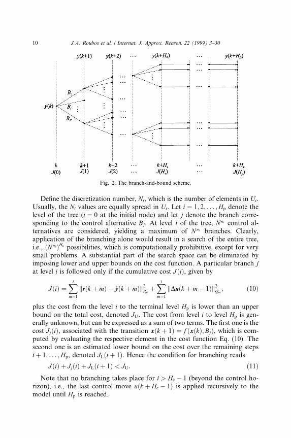
De®ne the discretization number, Ni, which is the number of elements in Ui.Usually, the Ni values are equally spread in Ui. Let i � 1; 2; . . . ;Hp denote thelevel of the tree (i � 0 at the initial node) and let j denote the branch corre-sponding to the control alternative Bj. At level i of the tree, Nni control al-ternatives are considered, yielding a maximum of N ni branches. Clearly,application of the branching alone would result in a search of the entire tree,i.e., �N ni�Hc possibilities, which is computationally prohibitive, except for verysmall problems. A substantial part of the search space can be eliminated byimposing lower and upper bounds on the cost function. A particular branch jat level i is followed only if the cumulative cost J�i�, given by

J�i� �Xi

m�1

kr�k � m� ÿ y�k � m�k2Pm�Xi

m�1

kDu�k � mÿ 1�k2Qm; �10�

plus the cost from the level i to the terminal level Hp is lower than an upperbound on the total cost, denoted JU. The cost from level i to level Hp is gen-erally unknown, but can be expressed as a sum of two terms. The ®rst one is thecost Jj�i�, associated with the transition x�k � 1� � f �x�k�;Bj�, which is com-puted by evaluating the respective element in the cost function Eq. (10). Thesecond one is an estimated lower bound on the cost over the remaining stepsi� 1; . . . ;Hp, denoted JL�i� 1�. Hence the condition for branching reads

J�i� � Jj�i� � JL�i� 1� < JU: �11�Note that no branching takes place for i > Hc ÿ 1 (beyond the control ho-

rizon), i.e., the last control move u�k � Hc ÿ 1� is applied recursively to themodel until Hp is reached.

Fig. 2. The branch-and-bound scheme.


The e�ciency of the bounding mechanism depends on the quality of thebound estimates. The upper bound should be as low as possible and the lowerbound as large as possible to decrease the number of branches. The availabilityof these estimates depends on the problem at hand. If no mechanism forcomputing the bounds is available, the upper bound is initially set to 1. The®rst path in the tree search exploits the `greedy' strategy of choosing thesmallest Jj�i� at each level i. When following a constant references or slowlychanging references, the terminal cost J�Hp� represents in most cases the op-timum, or a close upper limit of it. The upper bound is set to this value, i.e.,JU � J�Hp�. If at a later stage of the tree search, J�Hp�0 < JU is found, JU isreplaced by J�Hp�0. In the absence of a better estimate, the lower bound issimply set to JL�i� � 0 for all i � 1; 2; . . . ;Hc ÿ 1. Practical experience with thisalgorithm shows that even these `worst-case' estimates prevent the algorithmfrom exploring a large portion of the search space.

The branch-and-bound optimization technique applied to predictive controlhas three major advantages over other nonlinear optimization methods:

1. The global optimum (minimum in the above formulation) is always found(intrinsic property of the branch-and-bound method). This is a signi®cantadvantage, as it guarantees that the controller performs optimally in the dis-crete space of control alternatives, while no assumptions have to be madeabout the form of the cost function. Some issues connected with this discret-ization are discussed below.

2. The algorithm does not need any initial guess and hence its performancecannot be negatively in¯uenced by a poor initialization, as in the case of it-erative optimization methods.

3. The branch-and-bound method implicitly deals with constraints. In fact,the presence of constraints improves the e�ciency of bounding, as it restrictsthe search space by eliminating the control alternatives that result in violationof the constraints. Many other optimization techniques perform worse whentight constraints are imposed. The branch-and-bound technique also deals withdiscrete control alternatives in a natural way. In many industrial systems, someof the control variables are restricted to discrete values, which presents prob-lems for numerical techniques based on the computation or estimation ofgradients.This method has also two inherent disadvantages:

1. The computational e�ort is exponentially related to the search spacediscretization and the control horizon. In the case of MIMO processes, thesearch space increases very fast, e.g. for a 2� 2 MIMO systems with Hc � 5and a control discretization of n � 10, the number of possible control actions isalready �10�5��2 � 1010. This means that this method is generally not applicableto large systems in combination with a long control horizon.

2. The possible control actions are restricted to a set of discrete alternatives.Usually a large grid is used because of the related computational e�ort.However, the discretization of the control actions in branch-and-bound causes


a trade-o� between the number of discrete actions and the performance, i.e. a®ner grid gives a better approximation.In practice, several methods to reducethese disadvantages are proposed:

1. Iterative grid size re®nement [23], which has been successfully applied toDynamic Programming algorithms, is a method to reduce the computationale�ort when a small grid size is desirable, i.e., a small grid gives smoothercontrol signals and often a value of the optimum is found that is nearer to thereal optimum is found. A very rough grid size is chosen for discrete optimi-zation in order to reduce the computational e�ort. The obtained optimal set ofcontrol variables is used to initialize a new set B0, with a reduced grid aroundthe obtained optimal control. The grid size is reduced at every iteration bymeans of the grid size reduction factor c (%). The reduction factor c and thenumber of iterations nI , determine the ®nal grid size. SupposeB � f0; 2; 4; 6; 8; 10g, nI is 5, and c is 50, then the initial grid size is 2 andthe ®nal grid size is c�nI� � 2 � 0:55 � 0:03, which is 67 times smaller than at theinitialization. This method provides smooth control signals and prevents thesystem from oscillations between discrete alternatives due to a rough discret-ization. To gain maximal computational pro®t, one should ®nd an optimumbetween the number of discretizations, the reduction factor and the number ofiterations. A fast reduction will end up in a bad control around the one ob-tained after the ®rst iteration, while a slow reduction highly increases thecalculation e�ort.

2. A dynamic grid size is proposed by Sousa et al. [24] in order to keep thediscretization of the control low, while maintaining a good performance. Anadaptive set of discrete control alternatives, based on simple fuzzy criteria, isused. The adaptation is performed by a scaling factor multiplied by a dynamicset of control actions. In the proposed method fuzzy criteria are used for thepredicted error and the change of error. The aggregation of these criteria formsthe scaling factor. This method was able to calculate smooth control actionsand improve the performance for the simulation of a SIMO air-conditioningsystem. However, this method has not been extended for MIMO systems yet.

3. A `greedy' search often reduces the computational e�ort. After eachbranch, the objective function J�i� is calculated for all possible control actionsfor this step. These partial costs are sorted, such that the low cost possibilitiesare assigned a high priority during the search.

4. The last calculated sequence u�k; . . . ; k � Hp ÿ 1� at time k ÿ 1 is a goodestimate for the optimal sequence at time k when the reference trajectory isslowly changing. The output y�k � 1� can be calculated very fast for the esti-mated input and the accompanying J is used as Jmax in the branch-and-boundalgorithm.

5. E�cient computation of the objective value for several alternative inputs.The Takagi±Sugeno rule structure describes the in¯uence of the inputs on theoutputs. Often, several inputs are not included in the rules of some states.


Alternative inputs which are only di�erent in these variables will not in¯uencethe outcome of the state concerned. The computational load has been dimin-ished by detecting this type of rules and calculating the state only once.

The combination of methods 1, 2, 4 and 5 is used to reduce the computa-tional e�ort in the branch-and-bound algorithm that is being developed.Control results are presented in section 6.

5. Local linearization of Takagi±Sugeno model

Local linearization of Takagi±Sugeno fuzzy models is investigated in orderto extend the operating range of linear model-based predictive controllers [25].The fuzzy input±output model from Section 2 is linearized and rewritten into alinear time-varying state-space model. Here, the term `linearization' is used notin a Lyapunov sense but rather as freezing the time-varying components of theTakagi±Sugeno fuzzy model and thus obtaining a local linear model.

First, a single-step linearization approach is explained. Next, the single steplinearizing algorithm is extended with multiple linearizations in the predictionhorizon. Both algorithms lead to a time-varying incremental controller basedon LMBPC. First, the single-step linearization approach is explained.

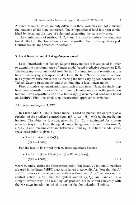
5.1. Linear state-space MBPC

In Linear MBPC [16], a linear model is used to predict the output y as afunction of the predicted control signal u�k; . . . ; k � Hp�, with Hp the predictionhorizon. The objective function, given by Eq. (6), is minimized for a givenreference trajectory. Here, the signal u may change over the control horizon Hc

�Hc6Hp� and remains constant between Hc and Hp. The linear model state-space description is given by

x�k � 1� � Ax�k� � Bu�k�;y�k� � Cx�k�: �12�

For the locally linearized system, these equations become

x�k � 1� � x�k� �A��x�k� ÿ x0� � B��u�k� ÿ u0�;y�k� � Cx�k� ; �13�

where x0 and u0 de®ne the linearization point. The local A�, B�, and C matricesare used in the linear MBPC algorithm (given in appendix A). Note that the A�

and B� matrices in the sequel are written without star (*). Constraints on thecontrol action �u;Du� and the system output (y;Dy� are handled in astraightforward way. The resulting QP problem can be solved e�ciently withthe MATLABATLAB function qp which is part of the Optimization Toolbox.


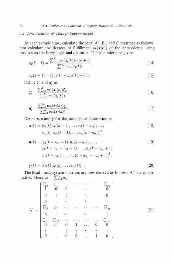
5.2. Linearization of Takagi±Sugeno model

At each sample time, calculate the local A�, B�, and C matrices as follows:®rst calculate the degrees of ful®llment xi�x�k�� of the antecedents, usingproduct as the fuzzy logic and operator. The rule inference gives:

yl�k � 1� �PKl

i�1 xli�xl�k��yli�k � 1�PKli�1 xli�xl�k��

; �14�

yli�k � 1� � �fliy�k� � gliu�k� � hli�: �15�De®ne f�l and g�l as:

f�l �PKl

i�1 xli�xl�k��fliPKli�1 xli�xl�k��

; �16�

g�l �PKl

i�1 xli�xl�k��gliPKli�1 xli�xl�k��

: �17�

De®ne x; u and y for the state-space description as:

x�k� � �x1�k�; x1�k ÿ 1�; . . . ; x1�k ÿ ny1�; . . . ; �18�xno�k�; xno�k ÿ 1�; . . . ; xno�k ÿ nyno��T;

u�k� � �u1�k ÿ nd1 � 1�; u1�k ÿ nd1�; . . . ; �19�u1�k ÿ nd1 ÿ nu1 � 1�; . . . ; uni�k ÿ ndni

� 1�;uni�k ÿ ndni

�; . . . ; uni�k ÿ ndniÿ nuni � 1��T;

y�k� � �x1�k�; x2�k�; . . . ; xno�k��T : �20�The local linear system matrices are now derived as follows: A� is a a1 � a1

matrix, where a1 �Pno

j�1 nyj:

A� �

f�1;1 f�1;2 . . . . . . . . . . . . f�1;a1

1 0 0 . . . 0

0 1 ... . .

.0

0 . . . . .. . .

. ...

f�2;1 f�2;2 . . . . . . . . . . . . f�2;a1

0 ... . .

. . .. ..

.

f�no;1f�no;2

. . . . . . . . . . . . f�no;a1

0 . . . 0 1 . . . 0 0

..

. ... ..

. . .. ..

. ...

0 . . . 0 0 . . . 1 0

2666666666666666664

3777777777777777775

; �21�


B� is a a2 � a2 matrix, where a2 �Pni

j�1 nuj:

B� �

g�1;1 g�1;2 . . . g�1;a2

0 . . . . . . 0

..

. ...

0 . . . . . . 0g�2;1 g�2;2 . . . g�2;a2

..

. . .. . .

. ...

g�no;1g�no;2

. . . g�no;a2

..

. . .. . .

. ...

266666666666664

377777777777775; �22�

and C is a no � a2 matrix:

C �1 0 . . . . . . . . . . . . 0

..

. . .. . .

. ...

0 . . . . . . 1 0 . . . 0

24 35: �23�

The C matrix is build as a zero-matrix where 1's are added such thatyl�k� � Cxl�k�.

5.3. Multi-step linearization

In the single-step linearization, a single linear model M�k� � fAk; Bk; Ckg isused over the entire prediction horizon at time instant k. For multiple-step-ahead control, however, the linear model may signi®cantly deteriorate from thenonlinear process and therefore negatively in¯uence the controllers perfor-mance. This can be overcome by using multiple linear models derived along theoperating trajectory within the prediction horizon, i.e. a sequence of modelsM�i� is obtained over i � k; . . . ; k � Hp. This procedure is called multi-steplinearization [26]. In the multi-step approach, it was not possible to use thesame time-invariant state-space representation as in the previous section. Thenew time-variant discrete state-space model is given by

x�k � 1� � x�k� �Ak�Dx�k�� Bk�Du�k��;y�k� � Ckx�k�; �24�

where x�k � 1� is the predicted state vector and Dx�k� and Du�k� are the changeof the state and input vector. Ak, Bk and Ck are time-variant state, input andoutput matrices of the model. This formulation can be written iteratively to aform in which predictions of the future process output can be done. At timeinstant k, both the state vector and future control increment sequence areknown. The future states are predicted by successive substitution:1. Use the already obtained linear model M�k� to compute the control signal

u�k� over the entire prediction horizon.


2. Take u�k� to compute ym�k � 1�.3. Linearize the Takagi±Sugeno model locally around ym�k � 1�; u�k�� to ob-

tain M�k � 1�.4. Use M�k� and M�k � 1�, to compute the new control sequence u over the en-

tire prediction horizon.5. Now take u�k� and u�k � 1� and compute ym�k � 2�.6. Linearize around ym�k � 2�; u�k � 1�� to obtain M�k � 2�.7. Use M�k�, M�k � 1� and M�k � 2� compute new control sequence u over the

entire prediction horizon.Steps 5±7 are to be repeated for i � k � 2; . . . ; k � Hp. Then, based on M�k�,M�k � 1�, . . ., M�k � Hp�, the ®nal control u is computed. There are two waysto calculate the control sequence u. At step 1, when only a model M�k� isavailable, u is obtained as in the single-step case. Hereafter a set of linearmodels fM�k � i�gHp

i�1 is used. The QP problem (Appendix A) is modi®ed asfollows:

minD~uf 1

2D~uTHD~u� cTDug; �25�

with

H � 2�RTu PRu �Q�;

c � 2�RTu PT�RxAkx�k� ÿ r��T; �26�

and the constraints on u, Du, and y:

KDu6x; �27�with

K �

IDu

ÿIDu

IHpm

ÿIHpm

Ru

ÿRu

Ru1

dRu

ÿRu1

ÿdRu

266666666666666664

377777777777777775; x �

umax ÿ Iuu�kÿ 1�ÿumin ÿ Iuu�kÿ 1�

Dumax

ÿDumin

ymax ÿRxAkx�k�ÿymin ÿRxAkx�k�

dymax ÿRx1Akx�k� � y�k�dymax 1 ÿ dRxAkx�k�

ÿdymin �Rx1Akx�k� ÿ y�k�ÿdymin 1 � dRxAkx�k�

2666666666666664

3777777777777775; �28�

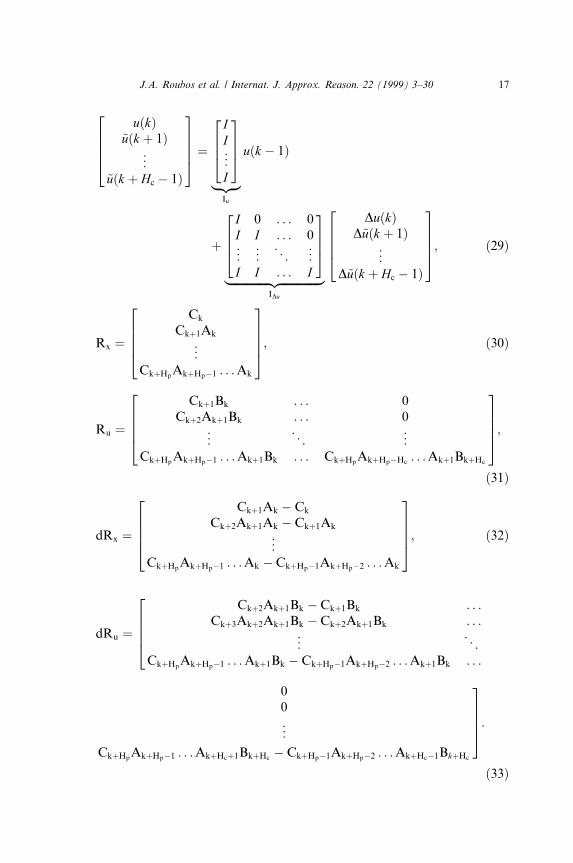
where IHpm is a �Hpm� Hpm� unity matrix. The matrices Iu; IDu;Rx;Ru; dRx anddRu, where ~u�k � i�, i � 1; . . . ;Hc ÿ 1 is the computed optimal control se-quence, are de®ned by:


u�k�~u�k � 1�

..

.

~u�k � Hc ÿ 1�

2666437775 �

II...

I

26643775

|�{z�}Iu

u�k ÿ 1�

�I 0 . . . 0I I . . . 0

..

. ... . .

. ...

I I . . . I

26643775

|��{z��}IDu

Du�k�D~u�k � 1�

..

.

D~u�k � Hc ÿ 1�

2666437775; �29�

Rx �Ck

Ck�1Ak

..

.

Ck�HpAk�Hpÿ1 . . . Ak

2666437775; �30�

Ru �Ck�1Bk . . . 0

Ck�2Ak�1Bk . . . 0

..

. . .. ..

.

Ck�HpAk�Hpÿ1 . . . Ak�1Bk . . . Ck�Hp

Ak�HpÿHc. . . Ak�1Bk�Hc

2666437775;�31�

dRx �Ck�1Ak ÿ Ck

Ck�2Ak�1Ak ÿ Ck�1Ak

..

.

Ck�HpAk�Hpÿ1 . . . Ak ÿ Ck�Hpÿ1Ak�Hpÿ2 . . . Ak

2666437775; �32�

dRu �Ck�2Ak�1Bk ÿ Ck�1Bk . . .

Ck�3Ak�2Ak�1Bk ÿ Ck�2Ak�1Bk . . .

..

. . ..

Ck�HpAk�Hpÿ1 . . . Ak�1Bk ÿ Ck�Hpÿ1Ak�Hpÿ2 . . . Ak�1Bk . . .

2666400

..

.

Ck�HpAk�Hpÿ1 . . . Ak�Hc�1Bk�Hc

ÿ Ck�Hpÿ1Ak�Hpÿ2 . . . Ak�Hcÿ1Bk�Hc

37775:�33�


The matrices dRx1 and dRu1 are de®ned as hypothetical ®rst rows in dRx anddRu: dRx1 � Ck and dRu1 � Ck�1Bk ÿ Ck.

6. IMC scheme

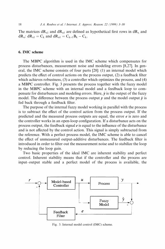
The MBPC algorithm is used in the IMC scheme which compensates forprocess disturbances, measurement noise and modeling errors [8,27]. In gen-eral, the IMC scheme consists of four parts [28]: (1) an internal model whichpredicts the e�ect of control actions on the process output, (2) a feedback ®lterwhich achieves robustness, (3) a controller which optimizes the process, and (4)a MBPC controller. Fig. 3 presents the process together with the fuzzy modelin the MBPC scheme with an internal model and a feedback loop to com-pensate for disturbances and modeling errors. Here, y is the output of the fuzzymodel. The di�erence between the process output y and the model output y isfed back through a feedback ®lter.

The purpose of the internal fuzzy model working in parallel with the processis to subtract the e�ect of the control action from the process output. If thepredicted and the measured process outputs are equal, the error e is zero andthe controller works in an open-loop con®guration. If a disturbance acts on theprocess output, the feedback signal e is equal to the in¯uence of the disturbanceand is not a�ected by the control action. This signal is simply subtracted fromthe reference. With a perfect process model, the IMC scheme is able to cancelthe e�ect of unmeasured output-additive disturbances. The feedback ®lter isintroduced in order to ®lter out the measurement noise and to stabilize the loopby reducing the loop gain.

Two basic properties of the ideal IMC are inherent stability and perfectcontrol. Inherent stability means that if the controller and the process areinput±output stable and a perfect model of the process is available, the

Fig. 3. Internal model control (IMC) scheme.


closed-loop system is input±output stable. If the system is not input±outputstable, but it can be stabilized by feedback, IMC can still be applied. Perfectcontrol means that if the controller is an exact inverse of the model, the controlis error-free.

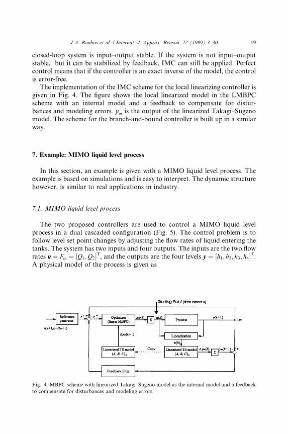
The implementation of the IMC scheme for the local linearizing controller isgiven in Fig. 4. The ®gure shows the local linearized model in the LMBPCscheme with an internal model and a feedback to compensate for distur-bances and modeling errors. ym is the output of the linearized Takagi±Sugenomodel. The scheme for the branch-and-bound controller is built up in a similarway.

7. Example: MIMO liquid level process

In this section, an example is given with a MIMO liquid level process. Theexample is based on simulations and is easy to interpret. The dynamic structurehowever, is similar to real applications in industry.

7.1. MIMO liquid level process

The two proposed controllers are used to control a MIMO liquid levelprocess in a dual cascaded con®guration (Fig. 5). The control problem is tofollow level set point changes by adjusting the ¯ow rates of liquid entering thetanks. The system has two inputs and four outputs. The inputs are the two ¯owrates u � Fin � Q1;Q2� �T, and the outputs are the four levels y � h1; h2; h3; h4� �T.A physical model of the process is given as

Fig. 4. MBPC scheme with linearized Takagi±Sugeno model as the internal model and a feedback

to compensate for disturbances and modeling errors.


_h �

ÿ S2;1

S1;1

��2gp

0 r3;1S2;3

S1;1

��2gp

r4;1S2;4

A1;1

��2gp

0 ÿ S2;2

S1;2

��2gp

r3;2S2;3

S1;2

��2gp

r4;2S2;4

A1;2

��2gp

0 0 ÿ S2;3

S1;3

��2gp

0

0 0 0 ÿ S2;4

S1;4

��2gp

26666664

37777775��hp

�

0 0

0 01

S1;30

0 1S1;4

266664377775Fin; �34�

where S1;j and S2;j are the inlet and the outlet area of tank j, g is the gravityconstant (equal to 9.81), ri;j is the restriction parameter from vessel i to vessel jand fin;j the water ¯ow into vessel j. In this case, the variables are chosen to be:

r3;1 r3;2

r4;1 r4;2

� �� 0:8 0:2

0:2 0:8

� �; �35�

S � 10ÿ3 10ÿ3 10ÿ3 10ÿ3

10ÿ6 10ÿ6 10ÿ6 10ÿ6

� �: �36�

Fig. 5. Liquid level process with four cascaded vessels.


The structure of the MIMO Takagi±Sugeno model is selected by using priorknowledge about the physical structure of the system as follows:

ny �1 0 1 10 1 1 10 0 1 00 0 0 1

26643775; nu �

0 00 01 00 1

26643775; nd �

0 00 01 00 1

26643775: �37�

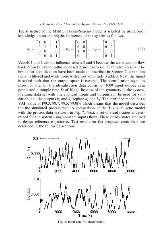
Vessels 1 and 2 cannot in¯uence vessels 3 and 4 because the water cannot ¯owback. Vessel 1 cannot in¯uence vessel 2, nor can vessel 3 in¯uence vessel 4. Theinputs for identi®cation have been made as described in Section 2: a randomsignal is ®ltered and white noise with a low amplitude is added. Next, the signalis scaled such that the output space is covered. The identi®cation signal isshown in Fig. 6. The identi®cation data consist of 1000 input±output datapoints and a sample time Ts of 10 (s). Because of the symmetry in the system,the same data set with interchanged inputs and outputs can be used for vali-dation, i.e., the outputs h1 and h3 replace h2 and h4. The identi®ed model has aVAF value of [99.3, 98.7, 99.5, 99.0]% which means that the model describesthe the simulated process well. A comparison of the Takagi±Sugeno modelwith the process data is shown in Fig. 7. Next, a set of steady states is deter-mined for the system using constant inputs ¯ows. These steady states are usedto design reference trajectories. Test results for the proposed controllers aredescribed in the following sections.

Fig. 6. Input data for identi®cation.


7.2. The branch-and-bound controller

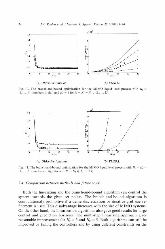
The branch-and-bound controller performance for the multi-tank systemusing a step-wise reference signal is shown in Fig. 8 and the correspondingcontrol input in Fig. 9. The used parameters are described in the caption ofthese ®gures. Figs. 10 and 11 show the in¯uence of the several parameters onthe performance. It can be seen that a discretization of 5 is necessary to obtainacceptable results. The computational load increases exponentially with thecontrol horizon. The control signal is ¯uctuates a great deal when a largediscretization is used without iterative grid size reduction. The result shown inFig. 9 is obtained when one uses iterative grid size reduction. The result is asmooth input signal. This option seems to be very powerful for systems withlong sample times. Second, it creates the possibility to calculate the maximalfeasible results o�-line for fast systems. These results can then be comparedwith other control methods, such as the local linearizing approach.

7.3. Local linearizing controller

Both linearization methods were tested in the proposed LMBPC structure.The controller is simulated for various set point changes with Hp � 5 and

Fig. 7. Comparison of the process output (solid line) with the fuzzy model (dashed±dotted line).


Hc � 3. First, a set of steady states is determined for the system using constantinputs. These steady states are used to make reference trajectories with setpoint changes. The feedback gain is set at 0.5. Simulation result for a referencetrajectory is given in Fig. 12(a). The weight matrices in Eq. (6) are P �diag��1; 1; 1; 1�� and Q � diag��0; 0��. The calculated control actions are givenin Fig. 12(b). The four outputs show that the controller using multi-step lin-earization performs better in all cases. The control signals are smoother as well.However, the computational load is Hp times higher than that of the single-stepmethod because the multi-step linearization method performs the linearizationaround each point within the prediction horizon.

Fig. 8. The branch-and-bound controller performance for a step-wise trajectory for the MIMO

liquid level process with Hp � Hc � 1;N � 3; c � 0:5 and nI � 5.

Fig. 9. Control input calculated by the branch-and-bound controller.


7.4. Comparison between methods and future work

Both the linearizing and the branch-and-bound algorithm can control thesystem towards the given set points. The branch-and-bound algorithm iscomputationaly prohibitive if a dense discretization or iterative grid size re-®nement is used. This disadvantage increases with the size of MIMO systems.On the other hand, the linearization algorithms also gave good results for largecontrol and prediction horizons. The multi-step linearizing approach givesreasonable improvement for Hc � 3 and Hp � 5. Both algorithms can still beimproved by tuning the controllers and by using di�erent constraints on the

Fig. 11. The branch-and-bound optimization for the MIMO liquid level process with Hp � Hc ��1; . . . ; 3� (numbers in ®g.) for N � N1 � N2 2 �2; . . . ; 25�.

Fig. 10. The branch-and-bound optimization for the MIMO liquid level process with Hp ��1; . . . ; 4� (numbers in ®g.) and Hc � 1 for N � N1 � N2 2 �2; . . . ; 25�.


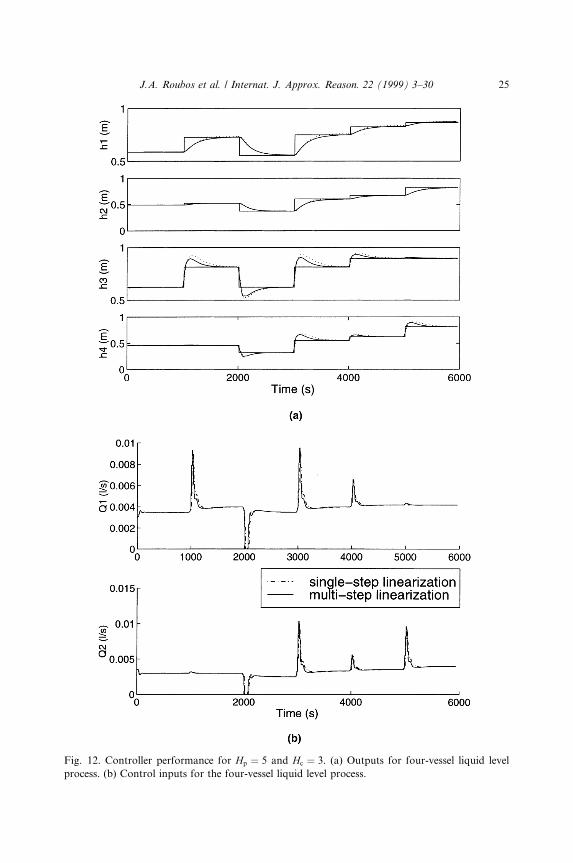
Fig. 12. Controller performance for Hp � 5 and Hc � 3. (a) Outputs for four-vessel liquid level

process. (b) Control inputs for the four-vessel liquid level process.


inputs and outputs. In the future, both methods will be tested at the two benchmarks of the FAMIMO project (see acknowledgements): (i) waste-watertreatment process, and (ii) direct-injection engine. The bench marks consist of areal system and a physical model simulation, which is used for the developmentof fuzzy control and fuzzy identi®cation algorithms. The waste-water treatmentprocess has two inputs and three states. Generally, the sample period is 15 min.Here, main problems are process disturbances and time-varying parameters.The second bench mark, the direct injection engine, has 3 inputs and 6 states.Here, a main problem is the short sample period of approximately 5 ms,necessary to control the system. Both methods will also be compared withother methods developed by partners in the FAMIMO project.

8. Conclusions

We have introduced the following optimization methods for MBPC withTakagi±Sugeno fuzzy models: (i) a branch-and-bound optimization strategy,and (ii) a local linear MBPC method. The linear MBPC method makes full useof the structure of the Takagi±Sugeno models (linear consequents) and is ef-®cient. The resulting QP optimization problem is being solved e�ciently whiletaking into account constraints on the output and control variables. This ap-proach shows good (but suboptimal) results for the presented examples. Thebranch-and-bound algorithm, on the other hand, always calculates the globaloptimum for the chosen discretization of the control space. Its major disad-vantage is the large computational power needed to arrive at the global solu-tion, especially for systems with many manipulated inputs. However, thebranch-and-bound method can always be used o�-line to calculate the maximalfeasible result. This solution can then be compared with other control methods,in this case the local linearizing approach.

Acknowledgements

This work has been done as part of the FAMIMO project funded by theEuropean Commission (ESPRIT LTR 21911). More information is availableat http://iridia.ulb.ac.be/FAMIMO/

Appendix A

Given the linear state-space system as described by Eq. (12) and the ob-jective function described by Eq. (6), the constrained Linear MBPC problemcan be solved by solving the quadratic program:


minD~uf 1

2D~uTHD~u� cTD~ug; �A:1�

with

H � 2�RTu PRu �Q�;

c � 2�RTu PT�RxA�k�x�k� ÿ r��T; �A:2�

and satisfying the constraints on u, Du, and y:

KD~u6x; �A:3�with

K �

IDu

ÿIDu

IHpm

ÿIHpm

Ru

ÿRu

26666664

37777775; x �

umax ÿ Iuu�kÿ 1�ÿumin ÿ Iuu�kÿ 1�

Dumax

ÿDumin

ymax ÿRxAx�k�ÿymin ÿRxAx�k�

26666664

37777775: �A:4�

IHpm is a �Hpm� Hpm� unity matrix. The matrices Rx;Ru; Iu; and RDu are de-®ned:

Rx �C

CA

..

.

CAHpÿ1

26643775; �A:5�

Ru �CB 0 . . . 0

CAB CB . . . 0

..

. ... . .

. ...

CAHpÿ1B CAHpÿ2B . . . CAHp ÿHcB

26643775; �A:6�

u�k�~u�k � 1�

..

.

~u�k � Hc ÿ 1�

2666437775 �

II...

I

26643775

|�{z�}Iu

u�k ÿ 1�

�I 0 . . . 0I I . . . 0

..

. ... . .

. ...

I I . . . I

26643775

|��{z��}IDu

�Du�k�

D~u�k � 1�...

D~u�k � Hc ÿ 1�

2666437775: �A:7�

Other constraints on u; y and x can be incorporated in a similar way [27].


Appendix B

Takagi±Sugeno rules for the four-vessel liquid level process:

Rules for output 1:1. If y1�k� is X11 and y3�k� is X12 and y4�k� is X13 then

y1�k � 1� � 9:68 � 10ÿ1y1�k� � 2:23 � 10ÿ2y3�k� � 5:81 � 10ÿ3y4�k� � 2:00 � 10ÿ3

2. If y1�k� is X21 and y3�k� is X22 and y4�k� is X23 then

y1�k � 1� � 9:76 � 10ÿ1y1�k� � 1:60 � 10ÿ2y3�k� � 3:33 � 10ÿ3y4�k� � 4:87 � 10ÿ3

3. If y1�k� is X31 and y3�k� is X32 and y4�k� is X33 theny1�k � 1� � 9:55 � 10ÿ1y1�k� � 3:46 � 10ÿ2y3�k� � 3:66 � 10ÿ3y4�k� ÿ 1:37 � 10ÿ4

Rules for output 2:1. If y2�k� is X11 and y3�k� is X12 and y4�k� is X13 then

y2�k � 1� � 9:66 � 10ÿ1y2�k� � 8:29 � 10ÿ3y3�k� � 2:76 � 10ÿ2y4�k� ÿ 1:37 � 10ÿ3

2. If y2�k� is X21 and y3�k� is X22 and y4�k� is X23 then

y2�k � 1� � 9:76 � 10ÿ1y2�k� � 4:91 � 10ÿ3y3�k� � 1:82 � 10ÿ2y4�k� � 7:74 � 10ÿ4

3. If y2�k� is X31 and y3�k� is X32 and y4�k� is X33 theny2�k � 1� � 9:46 � 10ÿ1y2�k� � 4:17 � 10ÿ3y3�k� � 6:66 � 10ÿ2y4�k� ÿ 1:48 � 10ÿ3

Rules for output 3:1. If y3�k� is X11 and u1�k� is X12 then

y3�k � 1� � 9:51 � 10ÿ1y3�k� � 9:43 � 103u1 �k� ÿ 5:15 � 10ÿ3

2. If y3�k� is X21 and u1�k� is X22 then

y3�k � 1� � 9:75 � 10ÿ1y3�k� � 9:24 � 103u1�k� ÿ 1:47 � 10ÿ2

3. If y3�k� is X31 and u1�k� is X32 theny3�k � 1� � 9:75 � 10ÿ1y3�k� � 8:72 � 103u1�k� ÿ 1:69 � 10ÿ2

Rules for output 4:1. If y4�k� is X11 and u2�k� is X12 then

y4�k � 1� � 9:36 � 10ÿ1y4�k� � 9:59 � 103u2�k� ÿ 3:60 � 10ÿ3

2. If y4�k� is X21 and u2�k� is X22 then

y4�k � 1� � 9:72 � 10ÿ1y4�k� � 9:19 � 103u2�k� ÿ 1:33 � 10ÿ2

3. If y4�k� is X31 and u2�k� is X32 theny4�k � 1� � 9:74 � 10ÿ1y4�k� � 9:37 � 103u2�k� ÿ 1:61 � 10ÿ2

References

[1] J. Richalet, Industrial applications of model based predictive control, Automatica 29 (1993)

1251±1274.

[2] J.M. Sousa, R. Babu�ska, H.B. Verbruggen, Fuzzy predictive control applied to an air-

conditioning system, Control Engineering Practice 5 (1997) 1395±1406.

[3] D.A. Linkens, S. Kadiah, Long-range predictive control using fuzzy process models, IChemE

74 (1996) 77±88.


[4] J. Valente de Oliveira, J.M. Lemos, Long-range predictive adaptive fuzzy relational control,

Fuzzy Sets and Systems 70 (1995) 337±357.

[5] U. Kaymak, J.M. Sousa, H.B. Verbruggen, A comparative study of fuzzy and conventional

criteria in model-based predictive control, in: FUZZ±IEEE, vol. 2, Barcelona, Spain, 1997,

pp. 907±914.

[6] Y.-Z. Lu, M. He, C.-W. Xu, Fuzzy modeling and expert optimization control for industrial

processes, IEEE Trans. Control Systems Technol. 5 (1997) 2±12.

[7] T. Takagi, M. Sugeno, Fuzzy identi®cation of systems and its application to modeling and

control, IEEE Trans. Systems, Man and Cybernetics 15 (1985) 116±132.

[8] B. Babu�ska, Fuzzy Modeling for Control, Kluwer Academic Publishers, Boston, 1998.

[9] B. Babu�ska, H.B. Verbruggen, Fuzzy set methods for local modeling and identi®cation, in:

R. Murray-Smith, T.A. Johansen, (Eds.), Multiple Model Approaches to Nonlinear Modeling

and Control, Taylor & Francis, London, 1997, pp. 75±100.

[10] M. Setnes, R. Babu�ska, H.B. Verbruggen, Rule-based modeling: Precision and transparency,

IEEE Trans. Systems, Man and Cybernetics, Part C: Applications & Reviews, 28(1) (1998)

165±167.

[11] I.M. Kouatli, A simpli®ed fuzzy multivariable structure in a manufacturing environment,

J. Intelligent Manufacturing 5 (1994) 365±387.

[12] Y.-Z. Lu, M. He, C.-W. Xu, Fuzzy modeling and expert optimization control for industrial

processes, IEEE Trans. Control Systems Technol. 5 (1997) 2±12.

[13] A. Gegov, Multilayer fuzzy control of multivariable systems by active decomposition, Int.

J. Intelligent Systems 12 (1997) 403±411.

[14] R. Babu�ska, J.A. Roubos, H.B. Verbruggen, Identi®cation of MIMO systems by input±output

TS fuzzy models, in: FUZZ±IEEE, vol. 1, Anchorage, Alaska, 1998, pp. 657±662.

[15] L. Ljung, System Identi®cation ± Theory for the User, Prentice-Hall, Englewood Cli�s, NJ,

1987.

[16] C.E. Garcia, D.M. Prett, M. Morari, Model predictive control: Theory and practice ± a survey,

Automatica 25 (1989) 335±348.

[17] J. Sj�oberg, Q. Zhang, L. Ljung, A. Benveniste, B. Delyon, P.-Y. Glorennec, H. Hjalmarsson,

A. Juditsky, Nonlinear black-box modeling in system identi®cation: A uni®ed overview,

Automatica 31 (1995) 1691±1724.

[18] R. Soeterboek, Predictive Control; A Uni®ed Approach, Prentice-Hall, Englewood Cli�s, NJ,

1992.

[19] E.F. Camacho, C. Bordons, Model Predictive Control in the Process industry, Springer,

Berlin, 1995.

[20] L.G. Mitten, Branch-and-bound methods: General formulation and properties, J. Oper. Res.

18 (1970) 315±344.

[21] Y. Nakagawa, A new method for discrete optimization problems, Electron. Comm. Jpn. 73

(11) (1990) 99±106.

[22] T. Ibaraki, Theoretical comparisons of search strategies in branch-and-bound algorithms, Int.

J. Comput. Inform. Sciences 5 (4) (1976) 315±344.

[23] R. Luus, Optimal control by dynamic programming using systematic reduction in grid size,

Int. J. Control 51 (1990) 995±1013.

[24] J.M. Sousa, M. Setnes, U. Kaymak, Adaptive decision alternatives in fuzzy predictive control,

in: FUZZ±IEEE, Vol. 1, Anchorage, Alaska, 1998, pp. 698±703.

[25] J.A. Roubos, R. Babu�ska, H.B. Verbruggen, Predictive control by local linearization

of a Takagi±Sugeno fuzzy model, in: FUZZ±IEEE, vol. 1, Anchorage, Alaska, 1998,

pp. 37±42.

[26] S. Mollov, R. Babu�ska, J.A. Roubos, H.B. Verbruggen, MIMO predictive control by multiple-

step linearization of Takagi±Sugeno fuzzy models, in: Proceedings on CD-ROM, AIRTC,

Arizona, USA, 1998.


[27] H.A.B. te Braake, Neural control of biotechnological processes, Ph.D. Thesis, Department of

Electrical Engineering, Delft University of Technology, Delft, The Netherlands.

[28] C.E. Garcia, M. Morari, Internal model control: A unifying review and some new results, Ind.

Eng. Chem. Process Des. Dev. 21 (1982) 308±323.


Documents

Fuzzy model-based predictive control using Takagi–Sugeno ...bme2.aut.ac.ir/~towhidkhah/MPC/seminars-ppt/89/FUZZYMPC-Chares… · Takagi–Sugeno fuzzy models are suitable to model