Western University Western University

Scholarship@Western Scholarship@Western

Electronic Thesis and Dissertation Repository

12-1-2011 12:00 AM

A System Dynamics Based Integrated Assessment Modelling of A System Dynamics Based Integrated Assessment Modelling of

Global-Regional Climate Change: A Model for Analyzing the Global-Regional Climate Change: A Model for Analyzing the

Behaviour of the Social-Energy-Economy-Climate System Behaviour of the Social-Energy-Economy-Climate System

Mohammad Khaled Akhtar, The University of Western Ontario

Supervisor: Slobodan P. Simonovic, The University of Western Ontario

A thesis submitted in partial fulfillment of the requirements for the Doctor of Philosophy degree

in Civil and Environmental Engineering

© Mohammad Khaled Akhtar 2011

Follow this and additional works at: https://ir.lib.uwo.ca/etd

Part of the Civil and Environmental Engineering Commons

Recommended Citation Recommended Citation Akhtar, Mohammad Khaled, "A System Dynamics Based Integrated Assessment Modelling of Global-Regional Climate Change: A Model for Analyzing the Behaviour of the Social-Energy-Economy-Climate System" (2011). Electronic Thesis and Dissertation Repository. 331. https://ir.lib.uwo.ca/etd/331

This Dissertation/Thesis is brought to you for free and open access by Scholarship@Western. It has been accepted for inclusion in Electronic Thesis and Dissertation Repository by an authorized administrator of Scholarship@Western. For more information, please contact wlswadmin@uwo.ca.

A SYSTEM DYNAMICS BASED INTEGRATED ASSESSMENT MODELLING OF GLOBAL-REGIONAL CLIMATE CHANGE: A MODEL FOR ANALYZING THE

BEHAVIOUR OF THE SOCIAL-ENERGY-ECONOMY-CLIMATE SYSTEM

(Spine title: System Dynamics Based Integrated Assessment Modelling)

(Thesis Format: Monograph)

by

Mohammad Khaled Akhtar

Graduate Program in Engineering Sciences Department of Civil and Environmental Engineering

A thesis submitted in partial fulfillment of the requirements for the degree of

Doctor of Philosophy

The School of Graduate and Postdoctoral Studies The University of Western Ontario

London, Ontario, Canada

© Mohammad Khaled Akhtar 2011

ii

THE UNIVERSITY OF WESTERN ONTARIO School of Graduate and Postdoctoral Studies

CERTIFICATE OF EXAMINATION

Supervisor ______________________________ Dr. Slobodan P. Simonovic

Examiners ______________________________ Dr. Craig Miller ______________________________ Dr. Clare Robinson ______________________________ Dr. Gordon McBean ______________________________ Dr. Evan Davies

The thesis by

Mohammad Khaled Akhtar

entitled:

A System Dynamics based Integrated Assessment Modelling of Global-Regional Climate Change: A Model for Analyzing the Behaviour of the Social-Energy-Economy-Climate System

is accepted in partial fulfillment of the requirements for the degree of

Doctor of Philosophy

______________________ _______________________________ Date Chair of the Thesis Examination Board

iii

ABSTRACT

The feedback based integrated assessment model ANEMI (version 2) represents the society-

biosphere-climate-economy-energy system of the earth and biosphere. The development of

the ANEMI model version 2 is based on the system dynamics simulation approach that (a)

allows for the understanding and modelling of complex global change and (b) assists in the

investigation of possible policy options for mitigating, and/or adapting to changing global

conditions within an integrated assessment modelling framework. This thesis presents the

ANEMI model version 2 and its nine individual sectors: climate, carbon cycle, land-use,

population, food production, hydrologic cycle, water demand, water quality, and energy-

economy. Two levels of the model are developed and presented here. The first one represents

the society-biosphere-climate-economy-energy system on a global scale (ANEMI version 2).

The second one is developed for a regional presentation of Canada (ANEMI_CDN). The

development of the Canada model is based on the top-down approach and various

disaggregation techniques. The disaggregation technique also extends the capability of the

ANEMI model version 2 in generating monthly data, while the model runs with yearly time

step. To evaluate market and nonmarket costs and benefits of climate change, the ANEMI

model integrates an economic approach, with a focus on the international energy stock and

fuel price, with climate interrelations and temperature change. The model takes into account

all major greenhouse gases (GHG) influencing global temperature and sea-level variation.

Several of the model sectors are built from the basic structure of the previous version of the

ANEMI model (version 1.2) developed by Davies (2009) and reported by Davies and

Simonovic (2010; 2011). However, they are integrated in a novel way, particularly the water

sectors. The integration of optimization within the simulation framework of the ANEMI

model version 2 is timely, as recognition grows of the importance of energy-based economic

activities in determining long-term Earth-system behaviour. Experimentation with different

policy scenarios demonstrates the consequences of these activities on future behaviour of the

society-biosphere-climate-economy-energy system through feedback based interactions. The

use of the model ANEMI version 2 and ANEMI_CDN improves both scientific

understanding and socio-economic policy development strategy.

iv

This thesis describes the model structure in detail and illustrates its use through the analysis

of three policy scenarios in both global and Canadian perspectives.

Keywords: system dynamics simulation; feedback; climate change; integrated assessment

modelling; society-biosphere-climate-economy-energy system; Earth-system model; water

resources management; disaggregation

v

DEDICATION

To my parents

vi

ACKNOWLEDGEMENTS

First of all, I would like to gratefully acknowledge my supervisor Professor Slobodan P.

Simonovic for his guidance and indispensable support in completing this research. I greatly

admire him for his accessibility and patience, his professionalism and scientific insight. I feel

honoured to have him as my supervisor. Thanks are also due to Professor Gordon McBean of

the Geography department and Professor Evan Davies of the University of Alberta for their

invaluable suggestions at different stages of my study period.

My special thanks go to our project partners from the Economics department at Western:

Ph.D. candidate Jacob Wibe, Professor Jim Davies and Professor Jim MacGee. We worked

together on the development of the energy-economy sector of the ANEMI model version 2

and without their support the research would not have reached this level.

I am grateful for the support of NSERC (Natural Sciences and Engineering Research Council

of Canada) through its Strategic Research Grant to Professor Slobodan P. Simonovic and his

collaborators, which funded development of the ANEMI model. I am gratified by my friends

in the FIDS office and in Civil and Environmental Engineering at Western, who provided

inspiration from time to time, and much-needed escapes from work: Shubhankar, Vasan,

Hyung, Pat, Shohan, Tarana, Dragan, Ponselvi, Angela, Lisa, Vladimir, Jordan, Dejan,

Samiran, Amin, and Abhishek. Thanks to my friends in London: Iftekhar, Shahed, Bahalul,

Zahid and Anis for helping me time to time which made my life easier.

I can not forget the support of my family and friends in Bangladesh who inspired me to

achieve my dreams. Deepest thanks to my younger brother and sister for their continuous

support as they are taking care of our parents in my absence. I can not also forget my mother-

in-law, whose visit to us eased our lonely life away from home. My deepest gratitude goes to

my parents for their unconditional sacrifice, encouragement, patience, continuous support

and prayer in every step of my life.

vii

I am absolutely convinced that I could not have completed my Ph.D. program without my

beloved wife and son. Their sacrifice, presence and smile have revived me every day for

tomorrow's struggles; they are the very reason why I am here and am striving.

Finally, I would like to acknowledge everybody who supported me and my family, and I

forgot to mention him/her. I pray to Allah, the mighty God, to make this work and the effort

of the past years fruitful for my family and me, here and in the day after. I, humbly, ask Him

for His forgiveness to the whole world.

viii

TABLE OF CONTENTS

CERTIFICATE OF EXAMINATION ........................................................................... ii

ABSTRACT ...................................................................................................................... iii

DEDICATION................................................................................................................... v

ACKNOWLEDGEMENTS ............................................................................................ vi

TABLE OF CONTENTS .............................................................................................. viii

LIST OF TABLES ......................................................................................................... xiii

LIST OF FIGURES ........................................................................................................ xv

CHAPTER 1 ...................................................................................................................... 1

1 INTRODUCTION ......................................................................................................... 1

1.1 Climate Change ....................................................................................................... 1

1.1.1 Global Climate Change ............................................................................... 2

1.1.2 Climate Change Research ........................................................................... 4

1.2 Global Climate Modelling ...................................................................................... 8

1.3 Regional Climate Modelling ................................................................................... 8

1.3.1 Benefits of Regional Climate Modelling .................................................... 9

1.3.2 Limitations of Regional Climate Modelling ............................................. 10

1.4 Climate Research in Support of Policy Development .......................................... 10

1.5 Research Objectives .............................................................................................. 13

1.6 Contributions of the Research ............................................................................... 15

1.7 Thesis Organization .............................................................................................. 16

CHAPTER 2 .................................................................................................................... 19

2 LITERATURE REVIEW............................................................................................. 19

2.1 Climate Change Modelling ................................................................................... 19

2.2 System Dynamics Simulation Modelling ............................................................. 22

ix

2.2.1 Brief History ............................................................................................. 25

2.2.2 Basics of System Dynamics Modelling .................................................... 26

2.2.3 Application of System Dynamics Modelling to Climate Policy Assessment

................................................................................................................... 28

2.2.4 Application of System Dynamics Modelling to Water Resources

Management .............................................................................................. 29

2.2.5 System Dynamics Modelling in Engineering ........................................... 32

2.3 Optimization ......................................................................................................... 35

2.3.1 Applications of Optimization .................................................................... 35

2.3.2 Most Used Optimization Energy-Economy Models ................................. 37

2.4 Integrated Assessment Modelling (IAM) ............................................................. 39

2.4.1 The Emergence of IAMs as a Science-Policy Interface ........................... 39

2.4.2 Classification of IAMs .............................................................................. 39

2.4.3 Application of Integrated Assessment Models ......................................... 40

2.4.4 Challenges for IAM Studies...................................................................... 49

CHAPTER 3 .................................................................................................................... 51

3 GLOBAL MODEL OF THE SOCIAL-ENERGY-ECONOMY-CLIMATE SYSTEM

...................................................................................................................................... 51

3.1 Description of Individual Model Sectors .............................................................. 52

3.1.1 The Climate Sector ................................................................................... 54

3.1.2 The Carbon Sector .................................................................................... 66

3.1.3 The Energy-Economy Sector .................................................................... 75

3.1.4 The Food Production Sector ..................................................................... 91

3.1.5 The Land-Use Sector ................................................................................ 98

3.1.6 The Population Sector ............................................................................. 103

3.1.7 The Water Resources Sectors ................................................................. 108

3.1.8 Sea-Level Rise ........................................................................................ 127

x

3.2 Feedbacks Between and Within Sectors ............................................................. 133

3.2.1 Feedbacks within the ANEMI Model Version 2 Water Sectors ............. 136

3.2.2 Feedbacks in the ANEMI Model Version 2 Non-Water Sectors ............ 140

3.2.3 Summary ................................................................................................. 144

CHAPTER 4 .................................................................................................................. 146

4 GLOBAL MODEL EXPERIMENTATION.............................................................. 146

4.1 ANEMI Model (version 2) Performance ............................................................ 146

4.1.1 Water Use................................................................................................ 148

4.1.2 Sea-Level Rise ........................................................................................ 150

4.1.3 Global Population ................................................................................... 151

4.1.4 Energy based CO2 Emissions and Energy Production ............................ 153

4.1.5 Gross Domestic Product (GDP) .............................................................. 157

4.1.6 Physical Characteristics of the Earth System.......................................... 158

4.1.7 Summary ................................................................................................. 167

4.2 ANEMI Model Version 2 Simulations ............................................................... 168

4.2.1 Carbon Tax Scenario............................................................................... 169

4.2.2 Increase Water Use Scenario .................................................................. 170

4.2.3 Food Production Increase Scenario ........................................................ 171

4.3 Global ANEMI Model (Version 2) Analyses Results ........................................ 172

4.3.1 Global Carbon Tax Scenario ................................................................... 172

4.3.2 Global Water Use Scenario ..................................................................... 179

4.3.3 Global Food Production Scenario ........................................................... 185

CHAPTER 5 .................................................................................................................. 192

5 REGIONAL MODEL OF THE SOCIAL-ENERGY-ECONOMY-CLIMATE

SYSTEM .................................................................................................................... 192

5.1 Description of Individual Sectors of the ANEMI_CDN Model ......................... 194

xi

5.1.1 The Population Sector ............................................................................. 194

5.1.2 The Land-Use Sector .............................................................................. 195

5.1.3 The Water Sectors ................................................................................... 196

5.1.4 The Food Production Sector ................................................................... 199

5.1.5 The Energy-Economy Sector .................................................................. 200

5.2 Disaggregation Procedure ................................................................................... 203

5.2.1 Temporal Disaggregation........................................................................ 203

5.2.2 Spatial Disaggregation ............................................................................ 205

5.2.3 Disaggregation Data Description ............................................................ 206

CHAPTER 6 .................................................................................................................. 209

6 REGIONAL MODEL EXPERIMENTATION ......................................................... 209

6.1 Regional ANEMI Model (ANEMI_CDN) Performance .................................... 209

6.1.1 Water Use................................................................................................ 209

6.1.2 Population ............................................................................................... 212

6.1.3 Land-Use ................................................................................................. 213

6.1.4 Energy-Economy .................................................................................... 214

6.2 Regional ANEMI Model (ANEMI_CDN) Analyses .......................................... 215

6.2.1 Canada Carbon Tax Scenario .................................................................. 216

6.2.2 Canada Water Use Scenario .................................................................... 219

6.2.3 Canada Food Production Increase Scenario ........................................... 223

6.3 Summary ............................................................................................................. 228

CHAPTER 7 .................................................................................................................. 230

7 OPTIMIZATION AND SIMULATION FOR THE INTEGRATED ASSESSMENT

MODELLING ............................................................................................................ 230

7.1 Optimization Simulation Model ......................................................................... 231

7.1.1 Optimization Problem Definition ........................................................... 232

xii

7.1.2 Model Structure and Application ............................................................ 234

7.1.3 Mathematical Formulation of the Optimization-Simulation Problem in

ANEMI Version 2 ................................................................................... 237

7.2 Limitations .......................................................................................................... 248

CHAPTER 8 .................................................................................................................. 250

8 DISAGGREGATION FOR REGIONALIZATION OF ANEMI MODEL .............. 250

8.1 Disaggregation Modelling .................................................................................. 252

8.1.1 Temporal Disaggregation........................................................................ 253

8.1.2 Spatial Disaggregation ............................................................................ 262

8.2 Performance Evaluation ...................................................................................... 263

CHAPTER 9 .................................................................................................................. 266

9 CONCLUSIONS ........................................................................................................ 266

9.1 Representation of the Past ................................................................................... 267

9.2 How the Future May Look Under Various Policy Choices ................................ 269

9.2.1 Carbon Tax Implementation ................................................................... 270

9.2.2 Increased Water Consumption ................................................................ 270

9.2.3 Increased Food Production ..................................................................... 271

9.3 Optimization Simulation of ANEMI Model ....................................................... 272

9.4 Regionalization ................................................................................................... 273

9.5 Adjudication ........................................................................................................ 274

9.6 Recommendations for Future Research .............................................................. 275

REFERENCES ............................................................................................................... 278

APPENDIX A: Important Definitions from Economics ................................................ 303

APPENDIX B: Atmosphere-Ocean Global Climate Models ......................................... 306

APPENDIX C: Data Processing of GCM‘s .................................................................... 315

CURRICULUM VITAE ................................................................................................. 332

xiii

LIST OF TABLES

Table 2.1: List of Integrated Assessment Models (most used) ............................................... 43

Table 3.1: Initial temperatures and configuration of ocean layers (°C and m, respectively) . 66

Table 3.2: Parameters of the flow through the terrestrial biosphere ....................................... 72

Table 3.3: Initial carbon stock and base surface density of NPP, σ(NPPj)0, values ............... 72

Table 3.4: Initial fossil fuel reserve (in trillion GJ) ................................................................ 90

Table 3.5: Transfer matrix of area between ecosystems (Mha yr-1

) in 1980 ........................ 100

Table 3.6: Major stocks of water, and values used in the ANEMI model version 2 (in km3)

............................................................................................................................................... 110

Table 3.7: Hydrologic flows and initial flow values used in the ANEMI model version 2 (in

km3 yr

-1) ................................................................................................................................ 111

Table 3.8: Treated wastewater reuse allocations to water use sectors (after Davies, 2007) . 122

Table 3.9: Summary of the ANEMI model modifications ................................................... 145

Table 4.1: Assessed global water withdrawals and consumption (in km3/yr) ...................... 149

Table 4.2: Projected global water withdrawals and consumption (in km3/yr) ...................... 149

Table 4.3: Comparison of historical global population (in billions) ..................................... 152

Table 4.4: Comparison of future global population (in billions) .......................................... 152

Table 4.5: Comparison of historical industrial emissions (in Gt C/yr) ................................. 155

Table 4.6: Simulated industrial emissions (in Gt C/yr) ........................................................ 157

Table 4.7: Global surface temperature change (in oC) .......................................................... 160

Table 4.8: Future global surface temperature change (in oC) .............................................. 161

xiv

Table 4.9: Global atmospheric CO2 concentration (ppm) .................................................... 163

Table 4.10: Future global atmospheric CO2 concentration (ppm) ........................................ 164

Table 4.11: Historical net primary productivity (NPP), 1980-2005 .................................... 166

Table 4.12: Future net primary productivity (NPP) .............................................................. 167

Table 5.1: Population by age-group of 1980 (DESA, 2011) ................................................ 195

Table 5.2: Initial land transfer matrix for Canada (Mha yr-1

, in 1980) ................................ 196

Table 5.3: Initial value for irrigated area and electricity production (1980) ........................ 198

Table 5.4: Assumed future fossil fuel discovery (Canada) in billion GJ .............................. 202

Table 5.5: GCM models used for the regionalization of the temperature and rainfall data . 208

Table 8.1: Monthly average temperature (Kelvin) of Canada .............................................. 264

Table 8.2: Comparison of the average temperature (Kelvin), Canada ................................. 265

xv

LIST OF FIGURES

Figure 3.1: ANEMI model version 2 structure ....................................................................... 54

Figure 3.2: Model structure of the comprehensive climate sector .......................................... 56

Figure 3.3: Model structure of the simplified climate sector (after Nordhaus, 1994) ............ 57

Figure 3.4: Causal loop diagram of the comprehensive climate sector .................................. 58

Figure 3.5: Causal loop diagram of the simplified climate sector .......................................... 59

Figure 3.6: Model structure of the ANEMI model version 2 carbon sector ........................... 67

Figure 3.7: CO2 solubility of ocean water (after Larryn et al., 2003) ..................................... 68

Figure 3.8: Causal loop diagram of the ANEMI version 2 carbon sector .............................. 69

Figure 3.9: Causal loop diagram of ANEMI energy-economy sector .................................... 77

Figure 3.10: Yearly food production (billion veg-eq-kg) ....................................................... 93

Figure 3.11: Model structure of the ANEMI version 2 food production sector ..................... 94

Figure 3.12: Causal loop diagram of the ANEMI version 2 food production sector.............. 96

Figure 3.13 Model structure of the ANEMI version 2 land-use sector .................................. 99

Figure 3.14: Causal loop diagram of the ANEMI version 2 land-use sector ........................ 101

Figure 3.15: Model structure of the ANEMI version 2 population sector ............................ 104

Figure 3.16: Causal loop structure of the ANEMI version 2 population sector ................... 105

Figure 3.17: Model structure of the ANEMI version 2 hydrologic cycle sector .................. 110

Figure 3.18: Causal loop diagram of the ANEMI hydrologic cycle sector .......................... 112

Figure 3.19: Model structure of the ANEMI version 2 water demand sector ...................... 115

xvi

Figure 3.20: Causal loop diagram of the ANEMI model version 2 water demand sector .... 117

Figure 3.21: Model structure of the ANEMI version 2 water quality sector ........................ 121

Figure 3.22: Causal loop diagram of the ANEMI model version 2 water quality sector ..... 123

Figure 3.23: ANEMI model version 2 structure ................................................................... 135

Figure 3.24: Feedback loops within ANEMI model version 2 water sectors ....................... 137

Figure 4.1: Comparison of global population projection ...................................................... 153

Figure 4.2: Comparison of heat energy production .............................................................. 154

Figure 4.3: Comparison of electric energy production ......................................................... 154

Figure 4.4: Comparison of industrial carbon emissions ....................................................... 156

Figure 4.5: Comparison of GDP per capita .......................................................................... 158

Figure 4.6: Comparison of atmospheric CO2 concentration ................................................. 165

Figure 4.7: Energy used to produce electricity ..................................................................... 172

Figure 4.8: Energy used to produce heat energy................................................................... 173

Figure 4.9: Global energy consumption................................................................................ 174

Figure 4.10: Global CO2 emissions from fossil fuel ............................................................. 174

Figure 4.11: Global atmospheric CO2 concentration ............................................................ 175

Figure 4.12: Global atmospheric temperature change .......................................................... 176

Figure 4.13: Global sea-level rise ......................................................................................... 176

Figure 4.14: Global population ............................................................................................. 177

Figure 4.15: Global food production .................................................................................... 178

xvii

Figure 4.16: Global water-stress ........................................................................................... 178

Figure 4.17: Global GDP change .......................................................................................... 179

Figure 4.18: Global available surface water ......................................................................... 180

Figure 4.19: Global water-stress ........................................................................................... 181

Figure 4.20: Global food production .................................................................................... 181

Figure 4.21: Global population ............................................................................................. 182

Figure 4.22: Global CO2 emissions from fossil fuel ............................................................. 183

Figure 4.23: Global atmospheric CO2 concentration ............................................................ 183

Figure 4.24: Global GDP ...................................................................................................... 184

Figure 4.25: Global atmospheric temperature ...................................................................... 184

Figure 4.26: Global sea-level rise ......................................................................................... 185

Figure 4.27: Global food production .................................................................................... 186

Figure 4.28: Global available surface water ......................................................................... 187

Figure 4.29: Global water-stress ........................................................................................... 187

Figure 4.30: Global population ............................................................................................. 188

Figure 4.31: Global CO2 emissions from fossil fuel ............................................................. 189

Figure 4.32: Global GDP ...................................................................................................... 189

Figure 4.33: Global atmospheric CO2 concentration ............................................................ 190

Figure 4.34: Global atmospheric temperature ...................................................................... 191

Figure 4.35: Sea-level rise .................................................................................................... 191

xviii

Figure 5.1: Map showing Canada and ROW with 10 by 10 degree grid size ...................... 207

Figure 6.1: Domestic water withdrawals (Canada) validation.............................................. 210

Figure 6.2: Industrial water withdrawals (Canada) validation.............................................. 211

Figure 6.3: Agricultural water withdrawals (Canada) validation ......................................... 211

Figure 6.4: Population of Canada (validation results) .......................................................... 212

Figure 6.5: Forest area (Canada) validation .......................................................................... 213

Figure 6.6: Cultivated area (Canada) validation ................................................................... 214

Figure 6.7: Real GDP per capita for Canada ........................................................................ 215

Figure 6.8: GDP per capita (Canada) .................................................................................... 217

Figure 6.9: Total energy used in the production of aggregate energy services (Canada) ..... 218

Figure 6.10: Industrial emissions from fossil fuel (Canada)................................................. 219

Figure 6.11: Available surface water (Canada) .................................................................... 220

Figure 6.12: Water-stress (Canada) ...................................................................................... 220

Figure 6.13: Food production (Canada) ................................................................................ 221

Figure 6.14: Population (Canada) ......................................................................................... 222

Figure 6.15: CO2 emissions from fossil fuel (Canada) ......................................................... 222

Figure 6.16: GDP (Canada) .................................................................................................. 223

Figure 6.17: Food production (Canada) ................................................................................ 224

Figure 6.18: Available surface water (Canada) .................................................................... 225

Figure 6.19: Water-stress (Canada) ...................................................................................... 225

xix

Figure 6.20: Population (Canada) ......................................................................................... 226

Figure 6.21: CO2 emissions from fossil fuel (Canada) ......................................................... 227

Figure 6.22: GDP (Canada) .................................................................................................. 227

Figure 7.1: Basic computational flow chart of the energy-economy sector of the ANEMI

model (ANEMI version 2 and ANEMI_CDN) ..................................................................... 237

Figure 7.2: Schematic view of simulation based optimization scheme ................................ 238

Figure 8.1: Monthly temperature comparison between analyzed and simulated data .......... 265

1

CHAPTER 1

1 INTRODUCTION

This thesis presents the ANEMI version 2 and the ANEMI_CDN: nine-sector global and

regional versions of an integrated assessment model that combines a system dynamics-

based simulation with a non-linear optimization procedure. (―ANEMI‖ is an ancient

Greek term for the four winds, heralds of the four seasons; here ANENI links physical

system such as the climate and hydrological- and carbon cycles with the socio-economic

systems that change them: the economy, land-use, population change, and water use and

quality). In representing the social-energy-economy-climate system, the two versions of

this model function to clarify the fundamental feedbacks among the system‘s interrelated

sectors. Hence the model helps to increase our knowledge of climate change and its range

of impacts, and to assist in the adaption of suitable policy strategies. The disaggregation

modelling approach that we have adopted allows the global model of the ANEMI version

2 to be converted into a regional version for Canada. The ANEMI_CDN can thus support

the attempts to achieve environmental and economic benefits for all Canadians.

1.1 Climate Change

The term climate usually brings to mind an average regime of weather. Here we are not

so much interested in particular climates as we are in the Earth‘s climatic system as a

whole. The climatic system consists of those properties and processes that are responsible

for any given climate and its variations. According to Berkofsky et al. (1981), the

properties of the climatic system can be broadly classified as thermal, which include the

temperature of the air, water, ice, and land; kinetic, which include the wind and ocean

currents, together with the associated vertical motions, and the motion of ice masses;

aqueous, which include the air‘s moisture or humidity, the cloudiness and cloud water

content, groundwater, lake levels, and water content of snow, land and sea ice; and static,

2

which include the pressure and density of the atmosphere and ocean, the composition of

the (dry) air, the oceanic salinity, and the geometric boundaries and physical constants of

the system. The complete climatic system therefore consists mainly of five physical

components: the atmosphere, hydrosphere, cryosphere, lithosphere, and biosphere.

The earth‘s climates have always been changing, and the magnitude of these changes has

varied from place to place and from time to time. In some places, the yearly changes are

so small as to be of minor interest, while in others the changes can be catastrophic. The

increasing evidence from paleoclimatic specimens shows that the earth‘s climates have

undergone long series of complex natural changes in the past. The further realization that

human activities could expedite the process has aroused great interest in the problems

related to climate change and variation.

The last twenty years has witnessed a growing scientific consensus that global warming

is underway. Within the scientific community, it is largely accepted that climate change

will have significant- and mostly negative- consequences for humankind.

1.1.1 Global Climate Change

Climate change has been a subject of intellectual interest for many years. What compels

our interest is the growing awareness of the relationship between climate change and our

social and economical stability. As the climate is always changing, scientific research

focuses on such questions as how large these future changes will be, and where and how

rapidly they will occur.

The atmosphere is a global commons that responds to many types of emissions and many

other kinds of changes from the surface beneath it. In turn, the economic and social

3

structures of human civilizations are sensitive to atmospheric changes. A major climate

change could conceivably destabilize a civilization‘s economic and social structure.

Civilizations depend on such factors as food production and water availability and these

factors implicitly depend on the climate. Unfortunately, our climate system is in trouble,

having warmed by over 0.7 degree Celsius in the last 100 years (Hare, 2009). Most of the

warming since at least the mid-twentieth century is very likely due to human activities.

Even after 20 years of international attention, emissions (GHGs, particularly CO2) from

fossil fuel burning and land-use change continue to grow rapidly. As a result, the

concentration of CO2 has not only increased; it now exceeds any value after continuous

instrumental measurement. This current trend of rising CO2 concentration in turn

increases the atmospheric temperature rapidly through radiative forcing.

Modern climate change appears to be on the point of exceeding the threshold of natural

variability. This is largely a result of human-induced changes in atmospheric composition

(Karl and Trenberth, 2003). The sources of these atmospheric perturbations include

emissions associated with energy use, urbanization and land-use changes. While many

uncertainties remain about the rate of climate change, it is indubitable that these changes

will be increasingly manifested in important and tangible ways: extremes of temperature

and precipitation, decreases of seasonal and perennial snow and ice extent, and sea-level

rise.

The climate system evolves in time under the influence of its own internal dynamics and

due to changes in external factors that affect climate (called ‘forcings’). External forcing

include natural phenomena such as volcanic eruptions and solar variations, as well as

human-induced changes in atmospheric composition. Solar radiation powers the climate

system. There are three fundamental ways to change the radiation balance of the Earth:

1) by changing the incoming solar radiation (e.g., by changes in Earth’s orbit or in the

Sun itself); 2) by changing the fraction of solar radiation that is reflected (called

‘albedo’; e.g., by changes in cloud cover, atmospheric particles or vegetation); and 3) by

4

altering the longwave radiation from Earth back towards space (e.g., by changing

greenhouse gas concentrations). Climate, in turn, responds directly to such changes, as

well as indirectly, through a variety of feedback mechanisms (Le Treut et al., 2007).

There is no doubt that the earth‘s climates have changed in the past and will change in the

future. Along with an extended database, climate change theory and dynamical models of

climate change must focus more on the determination of the climate‘s predictability.

1.1.2 Climate Change Research

For more than a decade, climate change has been the focus of much research and

analysis. Although we have considerable knowledge of the broad characteristics of the

climate, we are still having difficulties in understanding the major processes of climate

change. This compels climate change researchers not only to study each individual

component of the climatic system but also the world‘s oceans, the ice masses, the

exposed land surface and importantly, the socio-economic system. Only through such

studies can an integrated modelling approach make significant advances in understanding

the indefinable and complex process of climatic change. Despite the global implications

of the problem, the overwhelming majority of the researchers involved worldwide in

studying the problem and its possible solutions are from industrialized countries.

Participation of lesser-industrialized countries has been limited.

The Panel on International Meteorological Cooperation of the Committee on

Atmospheric Science first stated the need for an increased understanding of the physical

basis of the climate in 1966. This panel resulted in the formation of the Global

Atmospheric Research Program (GARP), which is devoted both to the study of the

physical basis of the climate and the task of extending weather forecasts with the

assistance of numerical models. GARP organized several important field experiments

including GARP Atlantic Tropical Experiment in 1974 and the Alpine Experiment

5

(ALPEX) in 1982. These field experiments contributed to major improvements in

Numerical Weather Prediction. GARP operates under the auspices of the World

Meteorological Organization and the International Geodetic and Geophysical Union.

In order to improve our understanding of the complex interactions between the climate

system, ecosystems and human activities, the research community develops and uses

scenarios. These scenarios are intended to plausibly portray the future state of

socioeconomic, technological and environmental conditions, the emissions of greenhouse

gases and aerosols, and the climate. The model-based scenarios used in climate change

research are developed using a sequential process focused on a step-by-step and time-

consuming delivery of information between separated scientific disciplines (Moss et al.,

2010). Currently, climate change researchers from different disciplines deal primarily

with four scenarios of future radiative forcing, where radiative forcing refers to the

change in the balance between incoming and outgoing radiation to the atmosphere caused

by changes in atmospheric constituents, such as carbon dioxide.

The General Circulation Model (GCM) is almost the same as a Global Circulation Model,

but it is used when dealing specifically with global climate change (CLIMAP, 2011). The

General Circulation Model takes into account the atmosphere, ocean movement and

many other chemical and biological factors that can be employed for weather forecasting,

understanding climate and predicting climate change. The two main types of General

Circulation Models are Atmospheric and Ocean models, but putting those together

produces a complete climate model. The connected complete system is often called as

'coupled' model. Scenarios are the future prediction by the coupled atmosphere-ocean

General Circulation Models (AOGCMs). In many cases AOGCMs are capable of

predicting regional climate change, at least to some extent.

6

It is the intersectoral aspects of climate change, at once socio-economic and

environmental, that makes it such a complex problem. Thus the economics of climate

change are even less well-understood than climate science, and in the latter uncertainties

remain in transport modelling of the greenhouse gas (GHG) pollutants through the

atmosphere and the effect of GHGs on the atmospheric components (atmospheric

temperature, ocean temperature, rainfall, and etc.). Nowadays, many aspects of climate

change are under studied in isolation. But at the same time many researchers are currently

combining the socio-economic part of climate change with the scientific aspect of climate

change for policy option analysis under projected climatic (climate change) conditions.

Such models are known as integrated assessment models (IAMs). Kelly & Kolstad

(1999) broadly define an integrated assessment model as any model that combines

scientific and socio-economic aspects of climate change primarily for the purpose of

assessing policy options for climate change control. Some examples are: Dowlatabadi

and Morgan (1995; 1993a), Kolstad (1996), Lempert et al. (1996), Manne, Mendelsohn,

and Richels (1995), Nordhaus (1994), and Peck and Teisberg (1992).

According to Weyant et al. (1996), an integrated assessment model is one that draws on

knowledge from research in multiple disciplines. Weyant et al. (1996) mentioned three

purposes of such models: (1) to assess climate change control policies (for example, the

computation of the optimal climate control policy), (2) to constructively force multiple

dimensions of the climate change problem into the same framework (for example, in

identifying the driving forces behind climate change by identifying to which sectors

climate change is most sensitive), and (3) to quantify the relative importance of climate

change in the context of other environmental and non-environmental problems facing

humankind (for example, in ranking the benefits of climate change control with

improving sanitation or improving medicine in developing countries).

Policy evaluation integrated assessment models consider the policy options on the socio-

economic, biospheric and climatic systems. These are also known as simulation models.

7

The other type of IAM is an optimization model. The IAM serves two purposes: (a) to

find the optimal policy which trades off expected costs and benefits of climate change

control or the policy which minimizes costs of achieving a particular goal, and (b) to

simulate the effect of an efficient level of carbon abatement on the world economy (Kelly

& Kolstad, 1999). Usually, policy evaluation models deal with a single exogenous

specified policy and estimate the effect of that policy on individual sectors, as well as the

combined effect on the projected future. In contrast, policy optimization models search

for optimal policy. While this is a complex process, these models produce simpler

representations at the sectoral level. So, the advantage of a policy evaluation model over

an optimization model is in its detailed description of the physical, economic and social

aspects of the very complex climate change problem. Therefore, these types of IA models

very much depend on the skill of the modeler in taking into account how consumers and

producers behave. Such models could face problems when dealing with scarce resources

or environmental constraints. On the other hand, an optimization model deals with

complex policies that are dependent on state variables and economic growth. The

optimization model therefore allows producers and consumers to determine

endogenously the optimal mix of GHG intensive and non-GHG intensive fuels given a

climate change control policy, while in the policy evaluation model requires the modeler

to specify exogenously the mix of fuel used.

In such a situation, a model that combines both optimization and simulation in a single

modelling environment can wipe out the disadvantages of these two different types of

modelling approaches. In this research, such a combined model, the ANEMI (ANEMI

version 2 and ANEMI_CDN), is developed to model feedback in the society-biosphere-

climate system.

8

1.2 Global Climate Modelling

Global climate is a result of the complex interactions between the atmosphere,

cryosphere (ice), hydrosphere (oceans), lithosphere (land), and biosphere (life), fueled by

the non-uniform spatial distribution of incoming solar radiation (Stute et al., 2001).

A general circulation model is developed on the basis of fluid dynamics and

thermodynamics and it describes the atmosphere and ocean in an explicit way. GCMs

(see Appendix B) provides a great opportunity to study the past, present and future

climatic system, including global ocean circulation (Stute et al., 2001).

Understanding historical events and processes (paleoclimatic period) is essential to

understand the interrelationship among different components of the biospheric system

and their feedbacks. This acquired knowledge forms the basis of the model development,

on which future climate forecasting is carried out.

The global modelling deals with the whole globe rather than only a part of the sphere and

acts like a big brother or a big picture thinker to the regional model, by providing it with

boundary conditions.

1.3 Regional Climate Modelling

Global climate models (GCMs) are the fundamental tools for understanding the climatic

system, whereas the regional climate models (RCMs) are developed to study more

9

detailed processes of regional to local conditions. The relatively high resolution and

details construction of RCMs enables the researcher to visualize key input to climate

impact studies and to deal with possible damages and opportunities related to climate

variability and change. Nowadays, regional climate models are used by a wide range of

scientific communities around the world. Both the regional and global models have more

or less the same objective of regional and global weather forecasting. Over the past 20

years, the development of regional climate models has led to increased resolution and

longer model runs. Applications of regional climate models span both the past and

possible future climates, facilitating climate impact studies, information and support to

climate policy, and adaptation.

As the climate doesn‘t have any geographic boundary, the climate in any one region is

affected by the rest of the globe. Boundary conditions consist of the information

produced when the large-scale circulation impinges on regional model domain. Where

the large-scale circulation is directed out of the domain, boundary conditions absorb the

regional climate models (RCMs) information. (Typically, a regional model does not

provide information back to a GCM.) These lateral boundary conditions apply along the

sides of the regional domain (Rummukainen, 2010).

1.3.1 Benefits of Regional Climate Modelling

The main potential of regional modelling is fine resolution. Higher resolution improves

the representation of any specific area such as a water body, rainfall, surface temperature,

mountain ranges, lakes, and estuaries, as well as other surface features. These give rise to

local or regional circulation and precipitation features, temperature modifications, winds,

and so on. Such higher resolution is beneficial for synoptic and mesoscale systems

analysis, the study of the climatic process, and providing input for impact studies.

10

1.3.2 Limitations of Regional Climate Modelling

The quality of a regional climate model is not only dependent on the boundary condition

but also the quality of the model itself. GCMs have the skill, but suffer from systematic

biases (Rummukainen, 2010). A systematic error in GCMs can easily hinder the model

improvement because of non-local processes. RCM evaluation is often done with so-

called perfect boundary condition simulations, where the boundary conditions are derived

from global meteorological analyses or reanalyses that are compilations of observed,

rather than simulated conditions.

Availability of suitable observational data limits model evaluation. Even though regional

climate models are run at relatively high resolution, they still suffer from resolution

(scale) problems, as point data sets are collected at meteorological stations, ocean buoys,

and such. This is a complication particularly for the evaluation of many kinds of

extremes, as climate data generated by RCMs (gridded data) are more homogenous in

space compared to observations (Rummukainen, 2010). Another important limitation is

the relatively high demand of computational resources which can put a limit on the

number, resolution, or length of RCM runs.

1.4 Climate Research in Support of Policy Development

The development of environmental policies is not an easy process. It requires an effective

science-policy interface. Without an effective link between the two domains, sound

evidence-based policies are difficult to achieve. The importance of science in policy is

specifically recognized in the Canadian federal government context. In A Framework for

Science and Technology Advice: Principles and Guidelines for the Effective Use of

Science and Technology Advice in Government Decision Making, it is stated:

11

Science advice has an important role to play by contributing to government decisions

that serve Canada’s strategic interests and concerns in areas such as public health and

safety, food safety, environmental protection, sustainable development, innovation, and

national security. The effective use of science advice may also contribute to Canada’s

ability to influence international solutions to global problems (Government of Canada,

2000).

At a national level, the development of science and policy linkages requires (at a

minimum) the perception among policy makers that a particular issue is of importance. In

both developing and developed countries, long-term global environmental issues have

typically been overshadowed by more pressing national and international issues. The de-

emphasis in political dialogue on climate change is therefore very common in many

countries and regions. Because of the lack of political interest in the issue, the progress in

our knowledge of climate has been due to diligence of the large number of climate

researchers.

From a scientific perspective, the development of the ANEMI model version 2

contributes to an increased understanding of climate change. It improves the

representations of the physical processes involved in the climate system and the carbon

cycle, and includes the socio-economic sectors and activities that govern interactions with

the biophysical system, especially those that influence or control anthropogenic

emissions. It applies the system dynamics simulation methodology, since it can both deal

with long term delays, multiple feedback processes, and other elements of dynamic

complexity and also provide for easy integration of scientific concepts of social, natural

and engineering sciences.

From a decision-making perspective, the ANEMI model version 2 and ANEMI_CDN

allow policymakers to test multiple policy-dependent scenarios in order to evaluate the

12

impact of the variables that a policy can affect. This will help policymakers (a) to

determine the beneficial effects of different climate change policies, (b) to improve the

ability of society to adapt to the detrimental effects of climate change, and (c) to avoid

the worst possible outcomes.

As per Popovich et al. (2010), the innovative aspects of the research on science policy

communication include the process by which the research team collected policy-related

information and how it interacted with the policy domain. While the technical model

development proceeded at the University of Western Ontario, key partners in the

Canadian federal government were involved from the departments of Environment,

Finance, Natural Resources, Fisheries and Oceans and Agriculture. These partners

remained engaged throughout the entire process of both the model (ANEMI version 2,

ANEMI_CDN) development and have provided useful guidance and feedback. Science

policy dialogue was established through the consultation sessions, workshops and direct

interviews (see Popovich et al., 2010).

The development of both ANEMI model version 2 and ANEMI_CDN, the system

dynamics simulation based integrated assessment model for analyzing behavior of the

social-energy-economy-climate system, relied heavily on policy interaction. Direct

communication with policy partners from the government was not only useful for

developing the technical aspects of the model, but also for demonstrating the value in

science-policy interaction. By establishing a two-way dialogue, both domains were better

able to understand the other‘s approaches, and to foster a synergy that led to the creation

of a useful policy tool.

13

1.5 Research Objectives

The global climate has been changing due to human activities and is projected to keep

changing even more rapidly. The consequences of climate change could be devastating,

with increased atmospheric greenhouse gas concentrations resulting in large-scale, high-

impact, non-linear, and potentially abrupt and irreversible changes in physical and

biological systems (Mitchell, 2009).

Global climate models offer the best approach to understanding the physical climate

system. At various resolutions, they capture the basic behaviour of the physical processes

that drive the climate. However, these models focus only on natural systems, and do not

represent socio-economic systems that affect and are affected by natural systems. The

most common approach to combining socio-economic and biophysical systems involves

applying projected trends (scenarios) to ‗drive‘ the climate model. But such an approach

disregards the existing dynamic feedbacks. This research tries to bridge such gaps by

deploying an integrated assessment modelling approach within a system dynamics

simulation framework.

The very first objective of this research work is to represent our social-energy-economy-

climate system through the ANEMI model version 2 development. This research aims to

provide improved representations of the physical processes involved in the climate

system and the carbon cycle compared to ANEMI model version 1, representations that

also include the socio-economic sectors and activities that govern interactions with the

biophysical system, especially those that influence or control anthropogenic emissions.

This will help to identify the importance of nonlinearities and feedbacks in determining

the behaviour of the social-energy-economy-climate system. The first question to be

addressed in this research is: How do the paths of climate, environmental, social and

economic variables appear when new sectors of food production, energy-economy, and

14

population are incorporated in the ANEMI model version 2 and feedbacks between the

energy-economy and the environment are more fully modeled?

The earlier version of the ANEMI model version 1 (developed by Davies (2007; 2009)

and later reported by Davies and Simonovic (2008; 2010)) runs at a global scale, where

the climate related regional impact assessment and resource management is not an option.

Under such condition a regional integrated assessment model ANEMI_CDN is developed

from the ANEMI model version 2 with disaggregation approach. Hence the second

objective is to provide the Canadian government with a scientifically credible tool useful

for policy: a system dynamics based model, connecting science, governance, economy,

energy, and the environment. Under this objective a more particular research question is

raised: What would the future path of the major variables of the socio-energy-economy-

climate system in Canada under different policy options and will they differ much from

the global perspective?

The previous version of the ANEMI model (version 1) was facing challenges in defining

better policy-oriented decision making regarding energy consumption. This difficulty was

related to the absence of a market clearing mechanism (see Appendix A) in the energy-

economy sector. For a dependable ANEMI model version 2, the integration of such a

mechanism becomes necessary, and this turns out to be the third objective of this research

work.

Finally, the fourth objective is related to the development of a methodology, which can

bring-in a time series downscaling (both temporal and spatial) capability in the

ANEMI_CDN model. Since the climate, carbon and part of the hydrologic cycle in

global scale, the regional model (ANEMI_CDN), which is specifically focused on

Canada, requires some kind of mechanism to connect those global sectors with its

regional sectors, so as to maintain the continuous feedback links throughout the

simulation period. A time series modelling approach, disaggregation modelling, is

15

implemented to explore the suitability, as well as to enhance the regionalization process

of the ANEMI_CDN model.

1.6 Contributions of the Research

In general, my research is focused on the development of an integrated assessment model

of the social-energy-economy-climate system. In this connection an earlier version of the

ANEMI model (version 1.2) structure has been utilized with the incorporation of new

important sectors along with required modification of the existing sectors. Moreover, a

regional version of ANEMI model (ANEMI_CDN) is developed specifically for Canada

in context of local climate change study. More specifically, my research contributions

are divided into several areas that include:

a) Nine-sector integrated assessment model (ANEMI version 2) for the

social-energy-economy-climate system

Integrated assessment research provides a useful foundation for the new generation of

climate change science. Even though current integrated assessment models have offered

an incredible value to date, evolving climate issues present new, substantial challenges.

The emerging decision environment now demands expanded tools that integrate all of

these historical considerations with explorations of the intersections with climate impacts

and adaptation. Recently, many integrated assessment models have shared a broad,

interdisciplinary approach to modelling global change that mostly focused on feedbacks

between their subsystems. These models: ANEMI (version 2), and ANEMI_CDN

however, consists of nine individual sectors with several elements, thousands of

interconnections (feedbacks), and some of the sectors are very new: energy-economy,

food production, and population. With such a versatile and wide range of sectors along

with enormous feedback linkage, these two ANEMI models provide a balanced,

comprehensive approach towards integrated assessment modelling.

16

b) Integration of optimization within the system dynamics simulation

framework

Apart from the simulation modelling, the optimization model is generally used in

analyzing complex decision making processes. The main advantage of an optimization

model is its ability to deal with hundreds of possibilities and figure out the optimal

decision within a short span of time and resources. The ANEMI version 2 and

ANEMI_CDN model introduces the integration of an optimization scheme within a

system dynamics simulation structure, where the optimal plan/path is updated at each

time step of the simulation interval. Therefore, with the introduction of such unique

integration approach (simulation based optimization) in the field of integrated assessment

modelling, both the ANEMI version 2 and ANEMI_CDN models are becoming more

robust and reliable.

c) Implementation of a suitable disaggregation technique within the system

dynamics simulation framework

The basic goal of disaggregation modelling is to allow the preservation of statistical

properties at more than one level. The important properties that are always desirable to

preserve at all levels are means, variables, the probability distribution of values, and some

covariances. The regionalization approach of the ANEMI_CDN model is basically a top-

down approach (also known as step-wise design), where both spatial and temporal

disaggregation is possible. Inclusions of such a disaggregation modelling technique offers

the ANEMI_CDN model an ambitious future in regionalizing the global model.

1.7 Thesis Organization

Chapter 1 presents an introduction to climate change, climate change research and

climate change modelling in both global and regional perspectives. The second part of

17

this chapter describes the research goal, as well as the contribution of the research under

feedback based integrated assessment modelling framework. An argument is made that

most climate change modelling is gradually moving towards this newer, more integrative

approach, as awareness grows of the need for a more comprehensive approach towards

global change research

Chapter 2 brings a narrative description of the different type of modelling, including

climate change modelling, system dynamics modelling, integrated assessment modelling

and optimization, along with their applications.

Chapter 3 explains all the important sectors of the global ANEMI model version 2. This

chapter also focuses on the feedback based interaction between and within different

sectors.

Chapter 4 includes ANEMI model version 2 experimentation including: performance

investigation, scenario formulation, simulation and analyses of simulated results.

Chapter 5 describes all the regionalized sectors of the regional model ANEMI_CDN

along with a brief description of the disaggregation procedure.

Chapter 6 deals with the regional model ANEMI_CDN experimentations through model

performance investigation, simulation and analyses of simulated results.

Considering the broad sectoral representation and level of complexity of the model two

additional chapters (Chapters 7 and 8) are added to deliver a clear understanding of the

research work.

Chapter 7 introduces the optimization procedure within the system dynamics simulation

framework. Therefore, with this integration approach many of the advantages of the

optimization are now incorporated into the system dynamics based simulation framework

of the ANEMI model.

Chapter 8 reviews the disaggregation methods and techniques. With such disaggregation

it becomes possible to disaggregate the time series data. In this research both spatial and

18

temporal disaggregation is carried out to regionalize the global rainfall and temperature

data for the regional model ANEMI_CDN.

Chapter 9 concludes the dissertation. It describes the overall success of the research in

addressing the objectives and related questions. The last part provides a set of

recommendations for future research.

Three appendices are included in the dissertation. Appendix A provides some important

definitions relevant to this research. A brief description on the atmosphere-ocean global

climate models are stated under Appendix B. Appendix C contains programming codes

for re-scaling (up-scaling the spatial data resolution) the temperature and rainfall data.

19

CHAPTER 2

2 LITERATURE REVIEW

This chapter reviews some of the literature related to climate change modelling, system

dynamics modelling, integrated assessment modelling and optimization procedures.

Nowadays there are numerous climate change models; they function to predict future

changes in climatic conditions and to help formulate mitigation policies. Integrated

assessment models are especially useful in these regards, since they can provide insight

into the interaction between different sectors of a larger system. The component models

of individual sciences (natural or social) cannot do this.

Integrated assessment models for the study of climate change developed within the field

of system dynamics modelling. A brief description of this development follows later in

this chapter. We will also review some existing optimization models for the energy-

economy sector. It is necessary to elucidate the application of optimization procedures

while selecting the set of decision variables in maximizing/minimizing the objective

function.

2.1 Climate Change Modelling

The scientific consensus on climate change is unambiguous; climate change is an

observable phenomenon with the potential for catastrophic impacts (IPCC, 2007a).

Climate change modelling is a scientific branch that developed through mathematically-

based formulations to enhance the understanding and prediction of future climate change.

Currently the global circulation model (GCM), with its detailed and extensive description

20

of physical processes, has acquired a good reputation within the scientific community.

GCMs are used to assess strategies for climate change mitigation and adaptation. A large

range of other models are used for estimating future warming and its impacts, costs of

climate change mitigation and the role of technology, as well as policy analyses: energy

models, integrated assessment models, and Earth system models.

The Integrated Assessment Society defines the integrated assessment (IA) ‗as the

scientific ‗‗meta-discipline‘‘ that integrates knowledge about a problem domain and

makes it available for societal learning and decision making processes‘ (TIAS, 2011).

Predicting future global climate change requires an interdisciplinary outlook that takes

into account the physical, social, and political sciences. So the sectors required to

understand climate science are: oceanography, atmospheric dynamics, vulcanology, solar

physics, carbon cycle analysis, radiation calculations, ice sheet modelling,

paleoclimatology, and atmospheric chemistry. Such a large number of sectoral

representations can help us to derive real policy-relevant insights (Harremoes and Turner,

2001; Hope, 2005; Schneider, 1997; Weyant et al., 1996).

In order to understand anthropogenic climate forcing (human-induced climate change)

and its effects on natural and human systems, the researcher must coordinate the

knowledge from numerous disciplines or fields of inquiry, including economics,

engineering, energy, agriculture, health sciences, epidemiology, ecosystems, water

resource management, coastal processes, fisheries, and coral reef ecology (Sarofim and

Reilly, 2011). Economists also employ multi-equation computer models in their approach

to climate change.

To the present day, the atmospheric dynamics community has largely employed highly

resolved GCMs that could not internally calculate how emissions would lead to

increasing concentrations, and that therefore required exogenous concentration pathways.

21

For a single 100-year projection, these models require roughly few months to complete

(Sarofim and Reilly, 2011). Integrated assessment model (IAM) developers are therefore

concerned with bringing together the different earth system components. Such models

should also need to be computationally efficient to solve 100-year integrations within a

few minutes.

As IAMs aim to integrate different disciplines, they run the risk of becoming extremely

complex (van Vuuren, 2011). The most obvious remedy for such excessive complexity is

to simplify the climate system and the carbon cycle, which in many IAMs consists of

only a few equations (Goodess et al., 2003). Despite the potential drawbacks, IAMs are

used to explore the socioeconomic and technological drivers of greenhouse gas emissions

and the policies for constraining these emissions from a long-term, global perspective.

Parson et al. (1997) mentions that the 1974 Climatic Impacts Assessment Program

(CIAP) was one of the first IAs in the global environmental field. It is a combined study

by six interdisciplinary teams of the chemical, societal, biological, and economic impacts

of stratospheric supersonic transport. Prominent integrated assessment models based in

the United States include EPRI's MERGE model, PNNL's MiniCAM model (currently

known as GCAM), and MIT's EPPA-IGSM (or just IGSM). Other commonly used

integrated assessment models are the AIM model (Japan), the IMAGE model (the

Netherlands), and the MESSAGE model (Austria). These models are designed to produce

estimates of global average greenhouse gas concentrations and temperature change that

are consistent with the full Earth system models, but with minimal computing

requirements and little regional detail. Among the economic focused models, DICE

(Hulme and Mahony, 2010) was the first (in 1979) to include a simple climate model, but

many others have since followed (Sarofim and Reilly, 2011). DICE coupled an economic

model to a simple carbon cycle model. While exploring the potentials of future climate

policies, the DICE model is then calibrated against GCMs along with a quadratic damage

function based on global mean temperature change.

22

Researchers also include both the biophysical and economic systems in their cost

assessments of climate protection. In IAMs this is done first by combining the important

components of biophysical and economic systems, and then converting them into a single

integrated system. Such an approach is capable of delivering a suitable framework that

can combine knowledge from a wide range of disciplines. As per IPCC (2001), ―these

models strip down the laws of nature and human behaviour to their essentials to depict

how increased GHGs in the atmosphere affect temperature, and how temperature change

causes quantifiable economic losses‖.

2.2 System Dynamics Simulation Modelling

A system is a combination of components, which act together in achieving a specific

objective. A component is a single functioning unit of a system (Ogata, 2004). Systems

are not limited to physical ones; the concept of a system can be extended to abstract

dynamic phenomena, such as those encountered in economics, transportation, population

growth, biology, and climate science.

A system is considered dynamic if its present output depends on past input. If it does not,

the system is considered static. System dynamics is a method of learning complex

processes. Like many other disciplines, system dynamics has witnessed various changes

in its philosophy, strategy, and technique, in the course of its ongoing evolution. Sterman

(2000) states:

'System Dynamics is fundamentally interdisciplinary. Because we are concerned with the

behaviour of complex systems, system dynamics is grounded in the theory of nonlinear

dynamics and feedback control developed in mathematics, physics, and engineering.

Because we apply these tools to the behaviour of human as well as physical and technical

systems, system dynamics draws on cognitive and social psychology, economics, and

23

other social sciences. Because we build system dynamics models to solve important real

world problems, we must learn how to work effectively with groups of busy policy makers

and how to catalyse sustained change in organizations’ (pp. 4-5).

The use of system dynamics modelling has been expanding at a faster rate, because of its

unique ability to represent the real world by drawing complex, non-linear feedback loops

between social and physical systems.

According to Pruyt (2006), ―system dynamics is not a philosophy, methodology or

method, and that it is more than just a theory of structure, set of techniques or tools.‖

A model is simply a representation or reconstruction of the real world, or, in other words,

a conceptual construction of an issue under investigation. The modeler is an observer

who, by the act of modelling, creates ‗a new world‘ (Schwaninger et al., 2008). By

compromising among adequacy, time, and cost of further improvement, it is possible to

achieve only a degree of confidence in a model. Forrester (1994) states that the mental

model that people operating in the real system almost always fall back on is the

competitive model. In his opinion, a system dynamics model creates much more clarity

and unity than prior mental models, and that the "adequacy" decision usually generates

little controversy among real-world operators who are constrained by time and budget.

It is obvious that an attempt to design a system should start with a prediction of its

performance before the system itself can be designed in drawing or actually built (Ogata,

2004). System dynamics modelling is based on a continuous feedback mechanism,

incorporating the hypothesis of causal connections of parameters and variables as a

functional form, which should be fully transparent rather than of the black box type. The

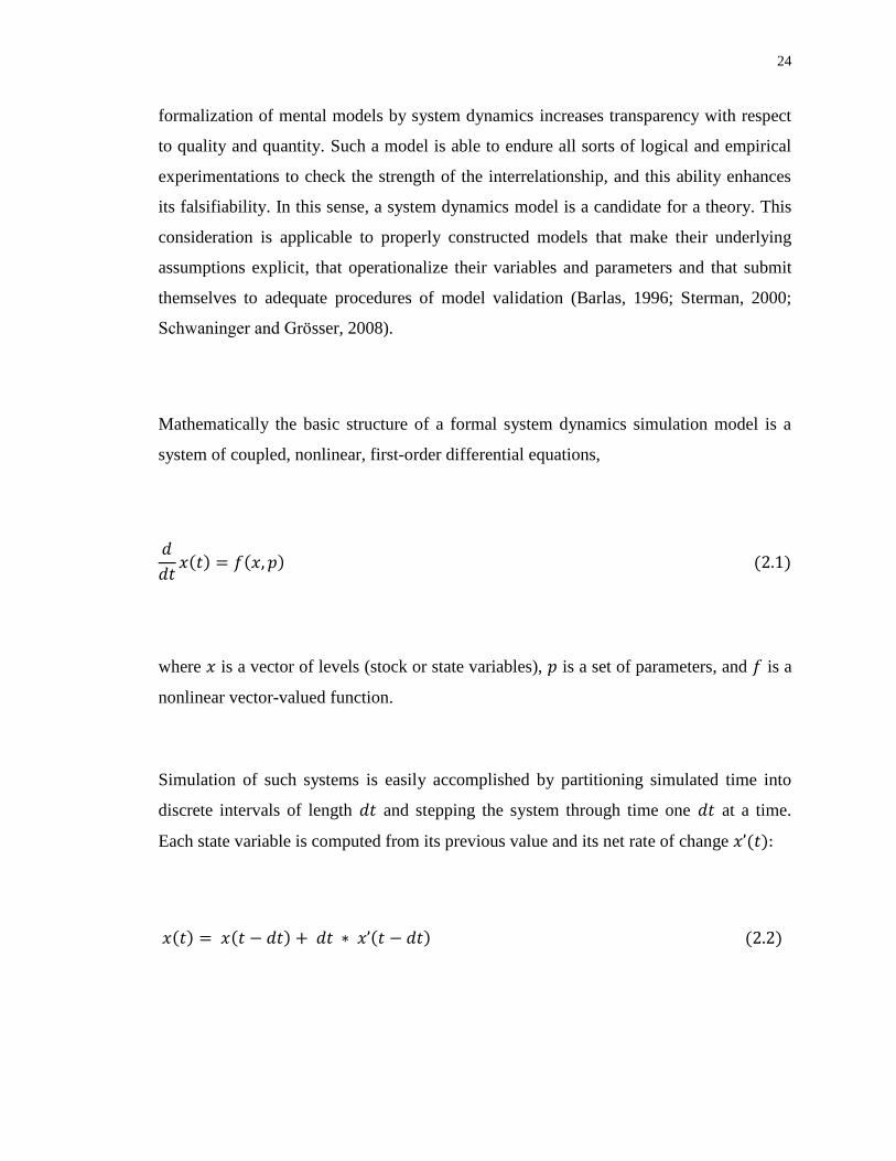
24

formalization of mental models by system dynamics increases transparency with respect

to quality and quantity. Such a model is able to endure all sorts of logical and empirical

experimentations to check the strength of the interrelationship, and this ability enhances

its falsifiability. In this sense, a system dynamics model is a candidate for a theory. This

consideration is applicable to properly constructed models that make their underlying

assumptions explicit, that operationalize their variables and parameters and that submit

themselves to adequate procedures of model validation (Barlas, 1996; Sterman, 2000;

Schwaninger and Gr sser, 2008).

Mathematically the basic structure of a formal system dynamics simulation model is a

system of coupled, nonlinear, first-order differential equations,

where is a vector of levels (stock or state variables), is a set of parameters, and is a

nonlinear vector-valued function.

Simulation of such systems is easily accomplished by partitioning simulated time into

discrete intervals of length and stepping the system through time one at a time.

Each state variable is computed from its previous value and its net rate of change

25

System dynamics modelling is engaged in building quantitative and qualitative models of

complex problems and then experimenting and analyzing the behaviour of these models

over time. Such models are often able to reflect the influence of unappreciated causal

relationships, dynamic complexity and structural delays which could lead to counter-

intuitive outcomes of less-informed efforts to improve the situation. The motivational and

perceptional scope of system dynamics modelling helps to manage engineering projects

in a more efficient and transparent way.

2.2.1 Brief History

System dynamics started at the Massachusetts Institute of Technology (MIT), Cambridge,

around 1958, under the pioneering leadership of Forrester (1958). Disappointed by the

prevailing approach and method of management science, which tended to view

management issues as isolated problems in isolated points in time, Forrester investigated

the question of how one could apply the concepts and ideas of Control Theory and

Control Engineering to management (Dash, 1994). It was a "remarkable leap of intellect"

(Coyle, 1989) when Forrester observed that these concepts and ideas can be made to

apply to management, and more generally to socioeconomic problems, in the same spirit

with which they are applied to designed physical systems, which constituted the original

subject matter of Control Theory. Industrial Dynamics (Forrester, 1961), Forrester's first

book, suggested the birth of system dynamics modelling as a discipline in its own right,

envisaging a considerable augmentation of the analytical strengths in the socioeconomic

field (Dash, 1994).

The field of application of system dynamics has changed since its initial development for

company policy making. Today, system dynamics methodology is used for other

problems as well. The modelling tools were originally developed with the clear intention

of facilitating the interplay between the manager‘s mental models and the analyst‘s

formal model. With time it seems that a huge opening has occurred in which system

26

dynamics modelling has become a prominent useful tool in the area of public policy.

According to Randers (1976), the continued prominence and usefulness of system

dynamics modelling may require that the special characteristics of the public policy scene

are recognized and allowed to influence the way in which policy studies are organized

and carried out.

2.2.2 Basics of System Dynamics Modelling

Much of the art of system dynamics modelling is discovering and representing the

feedback process, with stock and flow structures, time delays, and nonlinearities to help

determine the dynamics system (Sterman, 2000).

Feedback

Feedback is a process that occurs when the output of an event depends on the event‘s past

or future. Therefore, when any event is a part of a cause-and-effect chain and works as a

loop, the event is called a ―feedback‖ into itself (Simonovic, 2009). A feedback system

should have a closed-loop structure that brings results from the past action of the system

back to control future action. The basic example of a feedback system is a simple

thermostat that functions to maintain a constant temperature. The thermostat senses a

difference between desired and actual room temperature, and activates the heating unit.

The addition of extra heat helps to achieve the desired temperature and after achieving

the required level, the heating is turned off automatically until the room temperature

again falls below the desired one.

The actions of system actors can be basically of two kinds, which can be referred to as

negative and positive feedback effects. Those actions that attempt to control an

organization by introducing a balancing mode are called negative feedback (or self-

correcting) effects, and those that attempt to initiate growth in a reinforcing pattern are

27

called positive feedback (self-reinforcing) effects. Every system, from the very simple to

the most complex, consists of a network of positive and negative feedback. A system‘s

behaviour arises from the combined effect or interaction of these loops. Therefore, the

way that organizations respond to such actions is very important in developing and

understanding the system dynamics model.

Delay

Delays are a critical source of dynamics in nearly all systems. Some delays breed danger

by creating instability and oscillation. Others provide a clear light by filtering out

unwanted variability and enabling managers to separate signals from noise. Delays are

pervasive and take time to measure and report information. Sterman (2000) defines delay

as a process whose output lags behind its input in some fashion. The time delay is the

delay between the decision and its effects on the state of the system. Delay in the

feedback loops may create instability.

Stocks and Flows

Stocks are also called accumulations or states or levels. Stocks characterize the state of

the system and generate the information upon which decisions and actions are based.

Stocks give system inertia but also create a delay. A stock variable is measured at one

specific time, and represents a quantity existing at that point in time, which may have

accumulated in the past. Stocks change only over time and the value they possess at any

time depends on the value they have had on previous times.

28

The flow variables are also known as rates. A flow variable is measured over an interval

of time. Therefore, a flow is measured per unit of time. Flow is roughly similar to rate or

speed in this sense and is directly changing the levels/stocks. Flows are essentially the

same as auxiliaries and differ only in the way they are used in a model.

2.2.3 Application of System Dynamics Modelling to Climate Policy Assessment

The impact of IPCC in developing effective policies to combat climate change has been

marginal. This is because of the reliance on general equilibrium macroeconomic models

in the assessment of climate policies. In general the equilibrium approach is not capable

of capturing the dynamic feedback process. It also ignores other important aspects of

globalization, such as widespread poverty and growing rich-poor inequities associated

with migration pressures and increases in conflict potential. All of these aspects of

globalization need to be connected with the problem of global climate change.

The EU worked on the networking project ―Global Systems Dynamics and Policies‖ to

overcome the above mentioned deficiency by engaging itself in a network of researchers

cooperating in the development of a new generation of integrated assessment models

based on dynamical agent-based models. Specifically, the project's purpose was to review

how complex systems analysis can be applied to policy decisions, with a particular focus

on climate change, sustainable cities, risk, energy and social problems. Therefore, the

program aimed to connect the building of different methodologies of multi-physics

modelling, engineering systems, dynamics, economics and organizations modelling.

The standard general equilibrium paradigm of main-stream neo-liberal economics is

based on Adam Smith‘s famous ―invisible hand‖ in the Theory of Moral Sentiments. This

theory maintains that although the economy is governed by the diverse actions of

innumerable competing players, the net outcome is nevertheless an optimal equilibrium

29

state in which the integrated welfare of all players is maximized. Almost all the sectors of

the earlier version of ANEMI model (Davies and Simonovic, 2008; 2010) considered as a

nonlinear system with many degrees of freedom that is inherently chaotic, exhibiting

random fluctuations and heavily linked with feedback system. The inherent dynamics of

the socio-economic system and the important role of governments become particularly

relevant in the context of climate change.

It is also essential to understand the interrelations between climate change, energy and

climate change policies. This requires the application of a feedback-based system

dynamics model to simulate the behaviour of the key socio-economic factors. For an

effective communication between scientists and policymakers, the models should also

simplify their representations, making them easily understandable without looking at the

very inner equations. However, the implementation of the market clearance mechanism

in the economic sector demands the optimization approach. In such a situation, a

simulation based optimization model seems to be the only reliable tool to deal with the

implications of the assumptions regarding human behaviour and future technological

developments that are unavoidable in making climate policy decisions.

2.2.4 Application of System Dynamics Modelling to Water Resources Management

Over the last 50 years, system dynamics applications in Water Resource Management

(WRM) have branched off in many directions. Simonovic (2009) and Winz et al. (2009)

categorized these by their main problem foci: regional analysis and river basin planning,

urban water, flooding, irrigation and pure process models. So, the implementation of a

system dynamics methodology in finding a reasonable solution to a water resources

management related problem is not very new. The first comprehensive watershed model

(The Stanford Watershed Model) was developed by Crawford and Linsly in 1966.

However, Hamilton also developed the Susquehanna River Basin Model in the 1960‘s,

which was intended to describe the interdependencies between water resources and their

30

management on the one hand and quantifiable social and economic factors on the other

(Hamilton, 1969). Such a vast extension with respect to complexity and intersectoral

representation made the model very unique while costing increased data aggregation,

larger spatial scale, and computational time.

With time, the demand for regional analyses became a priority. In many cases, the

applications in regional analysis had a strong economic focus, examining feedback

relationships with industry but not much with available water resources. The use of

system dynamics as a tool for integrated regional analysis has been a continuing research

focus to the present. While discussing on the spatial scale Winz et al. (2009), mentioned:

Spatial scales have shifted from regional (Camara et al., 1986; Cartwright and Connor,

2003; Cohen and Neale, 2006; Connor et al., 2004; Den Exter, 2004; Den Exter and

Specht, 2003; Guo et al., 2001; Leal Neto et al., 2006; Passell et al., 2003; Sehlke and

Jacobson, 2005; Xu, 2001; Xu et al., 2002) to national (Simonovic and Fahmy, 1999;

Simonovic and Rajasekaram, 2004) to global (Simonovic, 2002a, b), so too have the

number of socio-economic factors included, mirroring improved computer capabilities as

well as changing problem foci (global water crisis and social impacts). Simonovic and

Rajasekaram (2004) note a recent trend in the reduction of spatial scales to basin and

watersheds with the aim of identifying regional and local solutions.

With increasing population and floodplain encroachment, the frequency of urban

flooding has increased. Water demand has started to increase as well. These factors pose

pressure for the management of urban water resources. The very strong and immediate

concerns of urban water resources management demands more model complexity and

thus the challenges facing model developers have increased. Due to the complex nature

of water transfer it is difficult for the modeler to define a spatial boundary. Moreover, the

integration of groundwater with surface water (Roach, 2007; Tidwell and Brink, 2008)

and irrigation practice took the flood management work one step ahead. In these areas of

31

research, models increasingly aim to investigate spatial outcomes (Ahmad and

Simonovic, 2004) and operational planning over shorter temporal scales.

Emerging in the late 1980‘s integrated water resource management (Bowden and

Glennie, 1986; Da Cunha, 1989; Rogers, 1993) not only acknowledges the integrated

nature of water resource problems but also the need to incorporate multiple objectives

and involve multiple stakeholders in the decision making process (Winz et al., 2009). As

Winz et al. report (2009), system dynamics model projects during the 1990s increasingly

incorporated participatory methods, particularly in the areas of regional analysis, and

regional and urban watershed management. Requests for participative adaptive

management were increasingly pronounced and legislation, such as the European Water

Directive, now prioritizes stakeholder participation in water management (European

Union, 2007). System dynamics models can be extremely helpful in facilitating

stakeholder participation.

Ahmad and Simonovic (2006) describe the development of a simulation tool for flood

management in the Red River basin near Winnipeg, Canada. Their intelligent decision

support system is intended for use as both a training tool for entry-level flood managers

and as an interactive problem-solving and advisory tool for experienced managers. In the

application, system dynamics constitutes one part of the overall modelling framework,

which also includes artificial neural networks, hydrological models, and geographic

information systems (GIS). Sehlke and Jacobson (2005) have also used system dynamics

to explore watershed management options for the Bear River basin, which runs through

Idaho, Wyoming, and Utah, in the North-western United States.

32

2.2.5 System Dynamics Modelling in Engineering

The objective of an engineering analysis of a dynamic system is to predict its behaviour

and performance. Real world dynamic systems are quite complex and often their exact

representation and analysis is not possible. However, making simplifying assumptions,

one can reduce the system model to an idealized version whose behaviour or performance

approximates that of the real system. The process by which a real physical system is

simplified to obtain a mathematically tractable situation is called the mathematical model

or simply the model of the system. System dynamics deals with the mathematical

modelling of dynamic systems in order to understand the dynamic nature of the system

and improve system performance.

System dynamics evolved from the field of systems science and control engineering. This

may give an impression that the field of control engineering is close in philosophy and

practice to system dynamics and system dynamics modelling. However, there is a

philosophical difference between control engineering and system dynamics; the concrete

applications and practice of the two fields appear totally different. In most cases, control

engineering is narrowly focused, whereas system dynamics are broad. In many cases

effective communication between managers and modelers are essential to develop

insights and implement system changes. Unfortunately, these participants in the

modelling and analysis are often unable to understand or use mathematical models.

System dynamics has a unique capability to overcome such constraints by its tools and

methods, which are effective with non-technical participants, as well as experienced

modelers.

Until now system dynamics has been applied in many complex social, environmental and

engineering systems (Lee et al., 2006), to model their respective problems. Much of the

early work of the group was concentrated in the field of production distribution system

design pioneered by Forrester (1961).

33

System dynamics is used in the power generation industry to understand the signals that

drive the installation of power generation capacity (Kadoya et al., 2005). Dyson and

Chang (2005) and Shelley et al. (2001) applied system dynamics to solid waste

management. Dyson and Chang (2005) also used it to develop a set of models for the

prediction of solid waste generation in a fast-growing urban setting.

Hughes (1971) studied the planning problem of a manufacturer of an item for the

Christmas market; because of the extreme seasonality of demand, the item had to be

produced throughout the year. Barnett (1973) considered the problem of how an oil

company should best develop a new oil field given that the initial development plans

were based on rather inaccurate estimates of basic parameters such as field size. The

Chemical Plant Investment cycle is one of a number of such cycles that is generally

recognized and whose effects on supplying industry are quite marked. Hill (1972)

constructed a preliminary model of the interactions between the chemical industry and

the design contractors and hardware suppliers that arise through chemical investment.

The first model of Coyle (1970) was an aggregate industry model designed to explore the

possibility of copper producers stabilizing prices via their production and stockholding

policies. It was found that the model of the existing production system gave rise to price

instabilities similar to those observed in practice. In his second model (1972), Coyle

examined the policies that an individual mining company might follow in order to

survive and grow in existing unstable markets.

System dynamics is also applicable in the construction industry. The system dynamics

based ‗change management system‘ of Lee et al. (2006) models the effects of

construction errors and plan changes on project durations. Ogunlana et al. (2003) also

used system dynamics to improve the organization and efficiency of large-scale, complex

construction projects in developing countries.

34

The trade cycle has a marked impact on demand for paper products, and the amplitude of

the cycle appears to increase as it moves up the chain from end user through the

merchants to the bulk producer. The paper industry is a major importer of costly and

scarce wood pulp. At the same time an increasing proportion of its raw material is drawn

from recycled waste paper. A Department of Industry funded project used a system

dynamics model to assess the impact of changes in technology on the industry and the

changes in management policies required to obtain the maximum benefit from them

(Price, 1975). System dynamics is also applicable in the shipping industry—disclosing,

for example, that the orders for new ships show a very marked cycle with a pronounced

boom, which generally lags increases in freight rates, followed by a long slump in which

very few orders are placed (Taylor, 1976a; Taylor, 1976b; Raiswell, 1976). Thus, system

dynamics models help to inform management in decision-making, in the capacity of what

Ahmad and Simonovic (2006) term decision support systems. It may be mentioned at this

point that the system dynamics is not just useful for resource management applications,

but has also been applied to improve understanding of basic physical characteristics and

processes.

According to Stave (2003: 304), the system dynamics approach is so broadly applicable

because it clarifies the problem under study, the behaviour of the resulting model, and the

real-world effects of potential solutions. The process of creating a simulation model helps

clarify the resource management problem and makes modellers‘ assumptions about the

way the system works explicit. Explaining the necessity of this kind of tool, Forrester

(1987) pointed out that while people are good at observing the local structure of a system,

they are not good at predicting how complex, interdependent systems will behave. Sehlke

and Jacobson (2005: 722) explain that system dynamics models allow the user to conduct

multi-scenario, multi-attribute analyses that resulting in relative comparisons over time of

many alternative management strategies.

35

Essentially, system dynamics is most useful for engineering applications where the

physical systems of interest are subject to strong social or economic influences (Xu et al.,

2002). From the above discussion it can be concluded that system dynamics is useful in a

variety of engineering fields: solid waste management, power generation, production,

shipping, utility planning, design, construction, and mining industry.

2.3 Optimization

The procedure of selecting the set of decision variables that maximizes/minimizes the

objective function subject to the system constraints is called the optimization procedure

(Simonovic, 2009). Until now, there has not been a single method that could be

applicable for solving all types of optimization problem in an effective way. Therefore,

various methods of optimization have been developed based on the characteristic of the

problem. Rao (1996) mentioned that the foundations of the calculus of variations, which

deals with the minimization of functionals, were laid by Bernoulli, Euler, Lagrange, and

Weirstrass. The optimum seeking methods are also known as mathematical

programming techniques and are generally studied as a part of operations research, a

branch of mathematics dealing with the application of scientific methods and techniques

to establish the best or optimal solutions (Rao, 1996). Operations research actually started

during World War II, when the British military was having problem in allocating their

limited resources (fighter planes, submarines, etc.).

2.3.1 Applications of Optimization

Optimization methodologies are being widely used in formulating energy system models.

An energy system optimization model can describe a large number of technical

components and can be used to find the best possible way to design and operate.

36

Linear programming has long been used as an optimization tool for energy system

modelling. In 1975, Singpurwalla used a LP model to minimize the system cost subject to

each energy source and air quality policy constraints (Jebaraj and Iniyan, 2006).

MARKAL is a linear programming model used to analyze minimum discounted cost

configurations for the Australian energy system during the period 1980–2020. Another

linear optimized model was used by Zhen (1993) to study long-term changes of the

system to a village level in the North China Plain. A linear programming model of an

integrated energy system for industrial estates (IESIE) was also developed around the

same time as a prefeasibility tool (Jebaraj and Iniyan, 2006). Macchiato et al. (1994)

developed a LP model for the planning of emissions abatement with a cost minimization

objective. Because of China‘s massive energy production from coal, Xie and Kuby

(1997) developed a strategic-level network based investment-planning optimization

model for a coal and electricity delivery system.

Taking the advantages of multidimensional optimization problems, Kaboudan (1989)

built up a non-linear dynamics econometric forecasting model to predict the electricity

consumption in Zimbabwe. Lai and Chen (1996) developed a MILP based model for

planning coal import strategies in Taiwan. Rozakis et al. (2001) also developed an

integrated micro-economic, multi-level mixed integer linear programming (MILP)

staircase model to estimate the aggregate energy supply at the national level.

Hoog and Hobbs (1993) proposed a multi-objective linear programming (MLP) model to

discuss issues including utility costs, emissions, regional economic effects, and net values

to customers. Another MLP model for energy capacity expansion was developed by

Climaco et al. (1995) where three conflicting objectives were considered, including net

present cost of expansion plans, reliability of the supply system, and environmental

impacts. Chedid et al. (1999) built up a fuzzy MLP model to deal with energy resources

allocation issues.

37

Bowe et al. (1990) introduced the use of a stochastic programming Markov model for

engineering-economic planning. Groscurth (1995) developed a model that describes

regional and municipal energy systems in terms of data-flow networks. A stochastic

version of the dynamics linear programming model was presented by Messner et al.

(1996). Davide et al. (2004) employed a stochastic method to establish a decision support

system for regional energy planning. In the following year Floros and Vlachou (2005)

developed a theoretical TSP model for analyzing energy demand and the effects of

carbon taxes on energy-related CO2 emissions.

2.3.2 Most Used Optimization Energy-Economy Models

There are many available optimization models that deal with the energy-economy sector.

A few of these are used in various long term projections undertaken in the international

community. These include the Model for Analysis of Energy Demand (MAED), PRIMES

energy system model, the Market Allocation (MARKAL) family of models, the Model of

Energy Supply Strategy Alternatives and their General Environmental Impacts

(MESSAGE), the World Energy Model (WEM), Modelling to Generate Alternatives

(MGA) and so on.

PRIMES energy system model was developed by the National Technical University of

Athens, Greece. It focuses on the market-related mechanisms that influence the evolution

of energy demand and supply, as well as the context for technology penetration in the

market. The PRIMES model is now used for projections, scenario construction and policy

impact analysis, with a forecasting horizon up to 2030 (Capros et al., 1998).

The Model for Analysis of Energy Demand (MAED) was originally developed by

Chateau and Lapillonne at the University of Grenoble, France. MAED provides a

38

methodical accounting framework for evaluating the effect on energy demand as a result

of changes in the technological and socio-economic system under analysis (IAEA, 2006).

The Market Allocation (MARKAL) family of models has contributed to energy-

environment planning since the 1980‘s. MARKAL is a widely used modelling tool and

its recognition relies on the fact that there are more than 150 teams in more than 50

countries using it (Mundaca et al., 2009).

The Model of Energy Supply Strategy Alternatives and their General Environmental

Impacts (MESSAGE) was developed at the International Institute for Applied Systems

Analysis (IIASA) in connection with its Environmentally Compatible Strategies (ECS)

programme (Mundaca et al., 2009). The model calculates an optimal and feasible energy

supply technology mix that requires the least total costs and meets a given useful or final

energy demand. In other words, MESSAGE determines the optimal solution

(Schrattenholzer, 2004).

Modelling to generate alternatives (MGA) can work as a way to flex energy models and

systematically explore the feasible, near-optimal solution space in order to develop

alternatives that are maximally different in decision space but perform well with regard to

the modelled objectives (DeCarolis, 2011). The MGA method allows modelers and

decision-makers to probe the decision space quickly and efficiently in order to identify

plausible alternative options.

The World Energy Model (WEM) has been utilized since 1993 by IEA for long-term

energy projections, mostly through the World Energy Outlook publication. The WEM

model has been coupled with a top-down General Equilibrium Model (GEM) called

IMACLIM-R to develop a hybrid modelling framework (Roques and Sassi, 2008). To

39

support the development of alternative policy scenarios, the IEA has built a database

containing more than 3,000 policies in OECD and non-OECD countries.

2.4 Integrated Assessment Modelling (IAM)

2.4.1 The Emergence of IAMs as a Science-Policy Interface

With the immense enhancement in computer technology, integrated modelling surfaced

in the mid-1980s as a new paradigm for interfacing science and policy concerning

complex environmental issues such as climate change. In the second half of the eighties,

it was believed that integrated modelling would be the optimal way to interface science

with policy. According to Parson (1994): ―To make rational, informed social decisions on

such complex, long-term, uncertain issues as global climate change, the capacity to

integrate, reconcile, organize, and communicate knowledge across domains - to do

integrated assessment - is essential.‖ Therefore, integrated assessment models are

believed to produce insights that cannot be easily derived from the individual natural or

social science component models that have been developed in the past (Weyant, 1994).

2.4.2 Classification of IAMs

Nowadays IAMs are capable of reflecting a range of modelling approaches that aim to

provide policy‐relevant information, and most can be summarized by: (i) policy

optimization that seeks optimal policies and (ii) policy evaluation models that assess

specific policy measures. The complexity of optimization models is limited, however,

because of the requirement of a large number of numerical algorithms in optimization.

Therefore these models tend to be based on compact representations of both the socio-

economic and natural science systems. They thus contain a relatively small number of

equations, with a limited number of geographic regions. Apart from policy optimization,

policy evaluation models tend to be descriptive and can contain much greater modelling

40

detail on bio-/geo-physical, economic or social aspects. These models are often referred

to as simulation models, and are designed to calculate the consequences of specific

climate policy strategies in terms of a suite of environmental, economic, and social

performance measures. An early example of this type of model is the Integrated Model to

Assess the Greenhouse Effect (IMAGE) by Rotmans (1990).

Other policy evaluation models include AIM, MESSAGE, etc. These models are not

subject to the constraints of optimization models, and therefore can incorporate greater

complexity in their representations of natural and social processes at the regional scale

without losing detail. Thus, they are generally applied to comparisons of the

consequences (e.g., regional economic and environmental impacts) of alternative

emissions scenarios. But even with these detailed descriptive capabilities, they are not

appropriate to optimize the economic activities of the energy-economy sector.

2.4.3 Application of Integrated Assessment Models

Integrated Assessment Modelling is usually comprehensive, but it produces less detailed

models than conventional climate- or socio-economic-centred approaches. It is based on

an understanding that feedbacks and interconnections in the society-biosphere-climate

system drive its evolution over time (Davies and Simonovic, 2008). Rotmans et al.

(1997b: 36), state that integrated assessments ―are meant to frame issues and provide a

context for debate. They analyze problems from a broad, synoptic perspective.‖

Integrated assessment modelling is not a new concept; it rather has a long history of

being applied to many problems. Over the past decade or so, integrated assessment

models (IAMs) have been widely utilized to analyze the interactions between human

activities and the global climate (Weyant et al., 1996). The first IPCC report referenced

two IAMs, the Atmospheric Stabilization Framework from US Environmental Protection

41

Agency (EPA) and the Integrated Model for the Assessment of the Greenhouse Effect

(IMAGE) model from the Netherlands (van Vuuren et al., 2006). These were employed

to assess the factors controlling the emissions and concentrations of GHGs over the next

century. MAGICC was then developed to account ocean heat transport and a carbon

cycle component to respond the land-use change; it is a multi-box energy balance model

(Meinshausen et al., 2008). Later, MAGICC modelling framework became a foundation

for the IPCC process, as it can easily show the climate implications of different emissions

scenarios and can be benchmarked to have climate responses that mimics those of any of

the GCMs.

Rotmans et al. (1997b) mention that the integrated assessment approach allows for an

exploration of the interactions and feedbacks between subsystems, and provides flexible

and fast simulation tools. It also identifies and ranks major uncertainties, and supplies

tools for communication between scientists, the public, and policy makers. Davies (2007)

provides some examples of integrated assessment models including the Integrated Model

to Assess the Greenhouse Effect, IMAGE 2.0 (Alcamo et al., 1994), the Asian Pacific

Integrated Model, AIM (Matsuoka et al., 1995), the Model for Evaluating Regional and

Global Effects of GHG reduction policies, MERGE (Manne et al., 1995), the Tool to

Assess Regional and Global Environmental and health Targets for Sustainability,

TARGETS (Rotmans and de Vries, 1997), the Integrated Global System Model, IGSM

(Prinn et al., 1999), Integrated Climate Assessment Model, ICAM (Dowlatabadi, 2000),

the Dynamics Integrated Climate-Economy model, DICE (Nordhaus and Boyer, 2000),

the Feedback-Rich Energy-Economy model, FREE (Fiddaman, 1997; Fiddaman, 2002),

and World3 (Meadows et al., 2004).

In Canada, an IAM platform evolved from a sub-basin or lake-ecosystem assessment tool

called RAISON (Regional Analysis by Intelligent Systems ON a microcomputer). Unlike

the policy driven IAM platforms such as RAINS, the Canadian version of IAM attempts

to balance the economy with the environment, or policy with science (Lam et al., 1994;

42

Lam et al., 1998). The Canadian IAM platform has been used as a decision-support

framework for basin management strategies on nutrient abatement, effluent limits, waste

disposal, dredging and other cleanup options in the Great Lakes 2000 program.

Information on hydrology, water quality, geology, fisheries, forestry, transportation,

urban development, socio-economy and health has been integrated in support of

watershed ecosystem research studies such as the Grand River Eco-Research Project.

Internationally, the RAISON system has been used for watershed modelling and lake

hydrodynamics for the Lerma-Chapala basin (Mexico) and the Lake Caohu basin in

China (Lam et al., 1994; Lam et al., 1998).

It has been predicted that global climate change will have significant impacts on society

and the economy, and that the adoption measures to tackle global climate change will

force the region to carry a very large economic burden. It is estimated that the greenhouse

gas emissions will increase to over one-half of total global emissions by the end of the

next century. The Integrated Assessment Model (IAM) provides a convenient framework

for combining knowledge from a wide range of disciplines; it is one of the most effective

tools to increase the interaction among these groups. A list of the important and widely

used IAMs is mentioned in the Table 2.1, followed by a brief description of each

individual model:

43

Table 2.1: List of Integrated Assessment Models (most used)

Model

Name

Author Type Field

AIM Morita et al. (1994) Evaluation Climate, water, agriculture, pollution,

socio-economic

DICE Nordhaus, W. D. (1994) Optimization capital, carbon, climate, population

FREE Fiddaman, T.S. (1997) Optimization Energy, economy, climate, carbon

ICAM Dowlatabadi & Morgan (1995) Evaluation Climate, energy, economy

IMAGE Alcamo (1994) Evaluation Landuse, climate, energy, sea-level

IGSM Prinn et al. (1999) Evaluation Economics, Climate, land ecosystems

MiniCAM Edmonds et al. (1994, 1996a) Optimization

& Evaluation

Energy, economy, agriculture, climate,

landuse

RICE Nordhaus & Yang (1996) Optimization Regional version of DICE model

TARGETS Rotmans et al. (1994, 1997b) Evaluation Population, energy, landuse, water,

economy

ANEMI

version-1

Davies and Simonovic (2008;

2010; 2011)

Evaluation Population, economy, landuse, water,

climate, carbon

AIM

The Asian-Pacific Integrated Model (AIM) is a dedicated Asia-Pacific regional model for

scenario analyses of greenhouse gas (GHG) emissions and the impacts of global

warming. Originally this large scale model was developed mainly to examine the global

warming response in the Asian-Pacific region, but later it became linked with a global

model to provide global estimates. The AIM is an integrated 'top-down and bottom-up'

model and comprises three main models: the greenhouse gas emissions model, the global

climate change model and the climate change impact model (Morita et al., 1994;

Matsuoka et al., 2001). The AIM model‘s time horizon is from 1990 to 2100 and consists

of nine regions: USA, Western Europe OECD and Canada, Pacific OECD, Eastern

Europe and Former Soviet Union, China and Central Planned Asia, South and East Asia,

the Middle East, Africa, Central and South America.

DICE

The DICE model, developed by William Nordhaus, is a dynamic integrated model of

climate change in which a single world producer-consumer makes choices between

44

current consumption, investing in productive capital, and reducing emissions to slow

climate change. Population growth and technological change yielding productivity

growth are both externally assumed to decline asymptotically to zero, eventually yielding

a stabilized population and productivity (Parson et al., 1997). The single consumer

maximizes the discounted present value of utility of consumption, which is subject to a

Cobb-Douglas production function that includes damages from climate change (CIESIN,

1995).

FREE

The FREE model is a single-region dynamic, disequilibrium model that includes learning

curves, economies of scale, and embodiment of technology and energy intensity

attributes in capital stocks. The FREE model represents the global energy-economy

system and, in a more limited fashion, global biogeophysical processes, where the

majority of the structure of the model is endogenous. Generation of economic output,

investment, energy supply and demand, depletion, and energy technology development

are tightly coupled to one another (Fiddaman, 2002). The FREE model is equipped with

endogenous carbon and energy tax policies, which is not very common in the IAMs.

However, non-energy based emissions (in this case CO2) and radiative forcing from other

greenhouse gases are treated exogenously.

ICAM

The Integrated Climate Assessment Model (ICAM) was developed to understand and

explore the interactions of different components of global atmospheric, economic and

demographic components, including energy resources. The ICAM model divides the

entire globe into 17 regions, each with its own population, economy, and policies for

responding to climate change (Dowlatabadi and Morgan 1993a; Dowlatabadi and Morgan

1993b; Lave and Dowlatabadi 1993). In many cases system dynamics based long-range

model projections might go beyond plausible results because of a lack in a sufficient

45

number of negative feedback loops. Such issues are dealt with in ICAM by incorporating

adaptive agents (entities that try to fulfill a set of goals in a complex, dynamic

environment).

IMAGE

Major land-use changes can influence bio-geochemical cycles. In this connection, the

Integrated Model to Assess the Greenhouse Effect (IMAGE) was developed under the

leadership of Jan Rotmans. Rotmans' determination and skill led to one of the first

integrated models of climate change, one that coupled calculations of energy, emissions,

climatic consequences and sea-level rise within a single framework. A second model,

IMAGE 2.0, evolved from developments in global change modelling that took place

during the 1980s at the International Institute for Applied System Analysis, Laxenburg,

Austria. In particular, the BIOME model (Prentice et al., 1992) and the RAINS (Regional

Air Pollution INformation and Simulation) model (Alcamo et al., 1990) contributed ideas

about rule-based simulations, process-based models applied on a geographic scale, and

spatial mapping, which led to the geographically explicit calculations of IMAGE 2.0.

IGSM

IGSM is an integrated global system model that is based on a set of coupled sub-models

of economic development, emissions, natural biochemical cycles, natural ecosystem and

the climate system (Prinn et al., 1999). One of the objectives of this model development

was to connect science and policy. In order to answer questions related to climate

uncertainties and climate feedbacks, and to examine a wide variety of policies, the model

attempts to address the major anthropogenic impacts and natural processes involved in

climate change (Schneider, 1992; Prinn and Hartley, 1992; IPCC, 1996).

46

Chemistry, atmospheric circulation, and ocean circulation are the essential components of

this model. IGSM consists of all the fundamental ecosystem processes in 18 globally

distributed terrestrial ecosystems. As per Prinn et al. (1999), IGSM has sufficient

biogeochemical and spatial detail to study both the impacts of changes in climate and

atmospheric composition on ecosystems, and the relationships between ecosystems and

chemistry, climate and natural emissions. The chemistry-climate treatment in IGSM

differs from other available assessment model frameworks. It incorporates highly

parameterized models of the climate system that do not explicitly predict circulation,

precipitation or detailed atmospheric chemistry, such as the MAGICC model (Wigley and

Raper, 1993; Hulme et al., 1995), the AIM model (Matsuoka et al., 1995), and the

IMAGE 2 model.

MiniCAM/ GCAM

The Mini Climate Assessment Model (MiniCAM), currently known as GCAM (Kim et

al., 2006), is a rapidly running Integrated Assessment Model that estimates global

greenhouse emissions with the Edmonds, Reilly and Barns (ERB) model (Edmonds et al.,

1994; 1996a) and the agriculture, forestry and land-use model (ALM) (Edmonds et al.,

1996b). The energy demand module initially estimates demands for three categories of

energy services (residential/commercial, industrial, and transportation) as a function of

price and income. For energy, emissions of CO2, CH4, and N2O reflect fossil fuel use by

type of fuel, while for agriculture, emissions of these gases reflect land-use change, the

use of fertilizer, and the amount and type of livestock produced. MiniCAM was first

developed with 11 regions but now includes 14 regions that provide complete world

coverage: USA, Canada, Western Europe, Japan, Australia and New Zealand, Eastern

Europe, Former Soviet Union, Latin America, Africa, Mid-East, China, India, South

Korea, Rest of South and East Asia.

47

RICE

The Regional Integrated model of Climate and the Economy (RICE) is a regional,

dynamic, general-equilibrium model of the economy that integrates economic activity

with the sources, emissions, and consequences of greenhouse-gas emissions and climate

change (Nordhaus and Yang, 1996). The RICE model takes a positive point of view by

asking how nations would in practice choose climate change policies in light of economic

trade-offs and national self-interests. In the RICE model, the world is divided into 10

different regions, but for the sake of simplicity they are often aggregated according to the

requirement. Each begins with an initial capital stock, population, and technology.

Population and technology grow exogenously, while capital accumulation is determined

by optimizing the flow of consumption over time. Output is produced by a Cobb-Douglas

production function in capital, labour, and technology. The major contribution of the

integrated approaches like the RICE model is to integrate the climate-related sectors with

the economic model (Nordhaus and Yang, 1996).

TARGETS

The Tool to Assess Regional and Global Environmental and health Targets for

Sustainability is TARGETS. This model includes five interlinked "horizontal" modules

representing population and health, energy and economics, biophysics, land and soils,

and water. TARGETS (Rotmans and de Vries, 1997) is a direct descendent of IMAGE. It

serves as a long term exploration of the at least partially unknowable dynamics of global

change that may shape the earth system over the next 100 years. The TARGETS

integrated framework basically consists of a population and health model, a

resources/economy model, a biophysics model, a land model and a water model, all of

which are interlinked (CIESIN, 1995).

The TARGETS model is not a traditional model insofar as it assumes that incremental

changes in parts of the global change system will cause gradual and incremental changes

in the system as a whole. The real world does not function in such a simple, linear way.

48

Therefore, TARGETS is a composite framework of simple systems (represented by

metamodels) that may show nonlinear and complex, perhaps even chaotic, behaviour

(Rotmans et al., 1994). This means that incremental changes in conditions of the

subsystems may result in considerable changes in the result of the overall system, which

may not always be predictable beforehand.

ANEMI (version 1)

ANEMI is a horizontally integrated assessment model that links climate change, water

resources and other physical and socio-economic issues to represent a larger society-

biosphere-climate system. It is based on circular references or ―feedbacks.‖ Such a basis

constitutes the major advantage of system dynamics modelling. In many isolated natural

science- or economically-based models, feedbacks are often treated as external qualities.

Thus, economic output and industrial emissions have been treated as extrinsic by natural

science models; climate change and the carbon cycle have been treated as extrinsic by

economically-based models; and population growth has been treated as extrinsic by both.

ANEMI explicitly models all of its feedbacks.

Originally introduced in 2007, the model underwent a moderate modification in 2009

(Davies, 2007; Davies and Simonovic, 2008; Davies and Simonovic, 2010). One can thus

make the distinction between version 1.1 and version 1.2. In version 1.1, the model

reproduces the major structural attributes of eight key components climate, carbon cycle,

economy, land-use, population, natural hydrological cycle, water use, and water quality

systems. (Davies, 2007; Davies and Simonovic, 2008). Version 1.2 adds an energy sector,

so as to include representations of the dynamics of energy supply and demand and carbon

emissions.

49

Analyzing the output from ANEMI version 1.2 is relatively straightforward. In terms of

modelling capabilities, it can simulate such effects in the climate and carbon systems as

changes in climate sensitivity parameters, as well as such effects in the land use and

economic sectors as the rate of land use change or the total factor productivity. However,

even with the energy sector, the ANEMI model version 1.2 has its limitations. With a

relatively simple representation of the macro-economic system, it cannot simulate

changes in primary and secondary energy supply and demand and it therefore lacks the

capacity to project a reasonable industrial emissions path.

2.4.4 Challenges for IAM Studies

The foremost challenge for IAM Studies is the integration of the natural and socio-

economic systems in order to better model the relationship between human activities and

the global environment. To the present, many integrated assessment models share the

same basic framework. Whether current IAMs have reached a level of development

where they can serve as the adequate basis for judgments in formulating actual global

environmental measures is debatable. Modellers appear to agree, however, that for the

most part the framework itself is acceptable. The integrated assessment of global

environmental issues from the perspectives of the natural and social sciences is not a field

of learning involving the pursuit of truth. Rather, it is a practical science that aims at

providing useful guidance to policy makers seeking to establish rules and policies that

help smooth the relationships between natural rule, the global environment and humanity.

Conventionally, it is possible to encapsulate the relationships between such practical

scientific studies and the real world in a relatively simple framework.

Any attempt to represent fully a complex issue and its numerous interlinkages with other

issues in a quantitative modelling framework is doomed to failure (Rotmans et al., 2001).

However, even a simplified integrated assessment model can provide valuable insight

into certain aspects of complex issues. Through their intersectoral links and

communication facilities, IAMs can provide more accurate representations of such

50

problems as climate change than those studies based a conventional modelling

framework. IAMs thus remain a very useful tool for decision makers, scientists–

especially in the field of climate change studies.

51

CHAPTER 3

3 GLOBAL MODEL OF THE SOCIAL-ENERGY-ECONOMY-CLIMATE SYSTEM

This chapter presents ANEMI version 2, the second version of a dynamic integrated

assessment model of the social-economic-climatic system. This model is an integrated

assessment model; it describes the major characteristics of the climate, carbon cycle,

land-use, water demand, water quality, natural hydrologic cycle, food production, energy-

economy, and population subsystems of the larger society-biosphere-climate-energy-

economy system.

ANEMI model version 2 builds on the ANEMI model version 1 (Davies, 2007; Davies

and Simonovic, 2008; 2009; 2010; 2011). It has been developed with the utilization of the

feedback based system dynamics simulation package, Vensim DSS (Ventana System,

2010a). New sectors have been incorporated (food production and population), while

existing sectors have been modified (water quality, water demand and climate). In the

ANEMI model version 2, a very significant modelling change has thus been implemented

in order to integrate a new economy-energy sector with other model sectors. The use of a

system dynamics simulation with embedded optimization makes ANEMI version 2 an

original integrated assessment tool. The integration process is supported through the use

of MATLAB (Math Works, 2011) and Visual studio (Microsoft, 1998) programming

tools.

In ANEMI version 2, the simulated values are based on the spatially aggregated

behaviour of the model components. Moreover, the key processes of all the sectors,

whether socio-economic or physical, are modeled at the global scale. Caution is therefore

required in downscaling simulated aggregate behaviour to local or regional scales. For

52

example, ANEMI model represents temperature change and atmospheric carbon dioxide

concentration as global variables. Important regional or local differences may thus elude

capture.

Each individual sector or sub-sector of the model describes the relevant dynamics of

individual system elements. ANEMI version 2 then links the individual model sectors

through mathematical feedbacks in order to describe the important existing dynamics of

the Earth-system as a whole.

The model simulation period ranges from 1980 to 2100. The model computational time

step is one year. This provides a long-term view of the feedback effects of global change,

albeit at the expense of daily and seasonal variation. Several components of the model are

original and several are based on available relevant models.

3.1 Description of Individual Model Sectors

The ANEMI model combines different sectors through feedback mechanisms in order to

capture the behavioural complexity of the socio-economic-climatic system. The

representation of all these sectors follows a structured approach. The model reproduces

the important elements or processes of the physical system in question rather than

simulating its behaviour through mathematical, pattern-matching type behaviour. This

structural approach allows for a more scientific representation of the feedback

relationships.

53

Version 2 of the ANEMI model represents each sector either in zero-dimensional or one-

dimensional form. Here, dimensionality refers to the degree of aggregation in a sector.

Zero-dimensional sectors model important characteristics and processes at a global-

aggregate level, while one-dimensional sectors have one spatial direction. For example,

the food production and population sectors produce single, global-aggregate values, and

so they are considered zero-dimensional. The oceans are modeled using vertical layers,

and the terrestrial biomes are separated into six components, and so they constitute one-

dimensional sectors.

The ANEMI model version 2 consists of nine sectors: climate, carbon cycle, energy-

economy, land-use, food production, population, hydrologic cycle, water demand, and

water quality. These sectors are of varying complexity. The land-use and population

sectors are relatively simple, while the carbon cycle and water-related sectors have much

more complex structures. Most importantly, a very sophisticated energy-economy sector

makes the ANEMI version 2 quite different from other, more conventional integrated

assessment models.

Figure 3.1 shows all of the sectors of the ANEMI model. The subsequent sections then

provide detailed descriptions of each sector.

54

Figure 3.1: ANEMI model version 2 structure

3.1.1 The Climate Sector

The climate sector of the ANEMI model version 2 simulates the atmospheric and oceanic

temperature changes caused by the increase in anthropogenic CO2 concentration. There

are two versions of climate sector in the ANEMI model version 2: one is the modified

form of ANEMI version 1 (for details see Davies, 2007; Davies and Simonovic. 2008),

basically based on the upwelling-diffusion energy-balance model (UD/EBM) that builds

on the Box Advection-Diffusion (BAD) model of Harvey and Schneider (1985a). The

second version of climate sector is based on the Nordhaus (1994) DICE model, which is

much simpler than BAD model.

Land Use

Energy-

Economy

Carbon

Climate

Hydrologic

Cycle

Population

+

WaterDemand

+

+

+

+

-

+

++

Land UseEmission

Clearing andBurning

Consumptionand Labour

Water Stress

Temperature

AtmosphericCO2

Industrial Emission

Total WaterDemand

WaterConsumption Surface Water

Availability

Water UseIntensity

Temperature

Water UseIntensity

Energy DemandIntensity

WaterQuality

WastewaterTreatment

WastewaterReuse

-

+

+

-

FoodProduction

+

Arable Land

+

Allocation forAgriculture

Water Stress

- Emission index

-

per capitafood

+-

Pollutionindex

Allocation forFertility control

-

++

Temperaturefeedback

-

+

Arable Land

Irrigationrequirement

55

According to Davies and Simonovic (2008), the main difference between the ANEMI

model version 1 (with its system dynamics based stock-and-flow structure) and the

original BAD model is the conversion of the climate sector from Harvey and Schneider‘s

(1985a) temperature based equations, using dT/dt, to an energy-based approach, with

energy stocks and flows, or E and dE/dt, measured in Joules, and Joules yr-1

.

The climate sector of the ANEMI model version 2 has a ‗switch‘, by which the modeler

can choose the complexity of the climate sector setup. The comprehensive setup is

adopted from the BAD model and includes detailed information on longwave radiation,

shortwave radiation, the temperature at different depths of the ocean, latent heat fluxes

and so on (Figure 3.2). Where, is the atmospheric heat capacity, is latent heat

flux, is climate sensitivity, is diffusivity constant, is the density of sea water,

is upward emittedsurface longwave radiation, is the downward emitted

longwave radiation, is the long wave radiation emitted to the space from top of the

atmosphere, is the shortwave (solar) radiation absorbed by the atmosphere, and

solar radiation absorbed by the Earth‘s surface.

56

Figure 3.2: Model structure of the comprehensive climate sector

The simplified setup of the climate sector (Figure 3.3) is based on the DICE model

(Nordhaus, 1994), and is used for computing atmospheric and oceanic temperatures.

Nordhaus used a second-order, linear system with three negative feedback loops. The

first loop describes the warming of the ocean while the remaining two describe the

transmission of heat from the atmosphere and ocean surface respectively.

As the ocean has a large heat capacity, deep ocean warming is a slow process. In this

model structure, radiative forcing from CO2 is expressed as a logarithmic function of the

atmospheric CO2 concentration. Forcing‘s from other gases are considered as exogenous

variables, based on the IPCC assumptions from the DICE model (Nordhaus, 1994). The

equilibrium temperature response to a change in radiative forcing is determined by the

radiative forcing coefficient and the climate feedback parameter.

OceanHeat

Diffusive Flow

K climate rho

Oceanic Mass

box depth

Ocean SurfaceArea

cp

AtmosphereHeat

Qs

Qa

L up L downLE and S

Heat

L out

Ra

Earth SurfaceArea

CurrentAtmosphericTemperature

RadiativeForcing

Advective Flow

Solar Constantchange

ForcingCalculation

Current OceanTemperature

57

Figure 3.3: Model structure of the simplified climate sector (after Nordhaus, 1994)

Causal Structure of the ANEMI Model Climate Sector

The causal loop diagram for the climate sector is presented in Figure 3.4 (comprehensive

version) and Figure 3.5 (simplified version).

In the ANEMI model version 2, the comprehensive climate structure computes the

atmospheric temperature from three sources: the radiation absorbed by the earth‘s

surface, latent heat flux, and upward surface radiation. In this setup the ocean has 20

layers and the heat is transmitted through advective processes (heat flowing through

global water upwelling) and diffusive processes (heat flowing downwards into colder

parts).

The simpler structure of the climate sector uses temperature gradient and the heat

absorption capacity of the deep ocean to represent the transmission of heat from the

AtmosphericUpper OceanTemperatur

Temperature difference

Feedback cooling

Climate feedback paramater

Heat transfer

Atmosphere and upper ocean heat capacity

Heat transfer coefficient

Radiative forcing

Deep OceanTemperature

Change in the atmosphere and upper ocean temperature

Change in deep ocean temperature

Deep ocean heat capacity

Heat capacity ratio

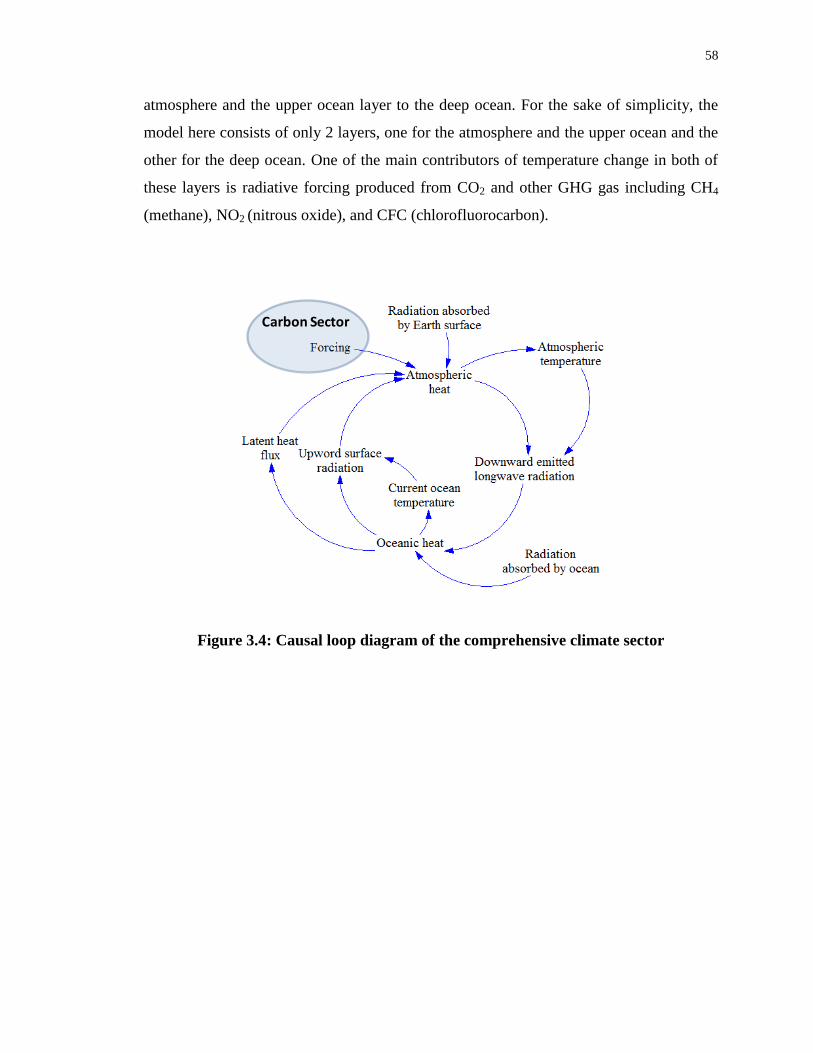
58

atmosphere and the upper ocean layer to the deep ocean. For the sake of simplicity, the

model here consists of only 2 layers, one for the atmosphere and the upper ocean and the

other for the deep ocean. One of the main contributors of temperature change in both of

these layers is radiative forcing produced from CO2 and other GHG gas including CH4

(methane), NO2 (nitrous oxide), and CFC (chlorofluorocarbon).

Figure 3.4: Causal loop diagram of the comprehensive climate sector

Carbon Sector

59

Figure 3.5: Causal loop diagram of the simplified climate sector

Mathematical Description of the ANEMI Version 2 Climate Sector

This section provides the major equations of the ANEMI version 2 climate sector, and

their associated parameters. Based on Harvey and Schneider (1985a) and later adopted

by Davies (2007), the key equations of this climate sector are: heat content of the

atmosphere (Equation 3.1), longwave radiation (Equations 3.2 to 3.4), sensible and latent

heat fluxes (Equations 3.5 and 3.6), heat balance of the mixed-layer and each ocean

layers (Equation 3.7 and 3.8), advective and diffusive flows between adjacent isothermal

layers (Equation 3.9 and 3.10). For the detailed description readers are advised to see

Davies and Simonovic (2008).

where is the heat content of the atmosphere (Joules), shortwave (solar) radiation

absorbed by the atmosphere, QA*, the upward emitted surface longwave (planetary)

Carbon Sector

60

radiation, L↑, the downward emitted longwave radiation, L↓, the longwave radiation

emitted to space from the top of the atmosphere, Lout, and the turbulent sensible heat

fluxes, H, latent heat fluxes, LE, and radiative forcing from anthropogenic greenhouse

gases, F.

For the downward longwave radiation emitted by the atmosphere,

where σ is the Stefan-Boltzman constant, TA is the current atmospheric temperature in

Kelvin, and ea is the atmospheric vapour pressure.

The upward longwave radiation calculation is modelled as the blackbody radiation from

the Earth‘s surface, where TS is the surface temperature.

The longwave radiation to space,

61

where, A, B, C are constant having values -251 W/m2, 1.8 W/(m

2 K), and 1.73 W/(m

2 K)

respectively. FCL represents the area-weighted mean annual cloud amount and ΔTS,CL is

the surface to cloud-top temperature difference.

The sensible and latent heat fluxes are,

where C1 and C2 equals 12.57 W/(m2 K) and 11.75 W/m

2 per mbar respectively. Here, es

is the surface saturation vapour pressure, TS surface temperature, and ea is the

atmospheric vapour pressure.

The heat balance of the mixed-layer is,

where, the solar radiation absorbed at the Earth‘s surface, QS*, the upward advective heat

flow in the oceans, Fadv, and the downward diffusive heat flow in the oceans, Fdiff.

62

The heat balance for each ocean layer in the model is given by,

where HO(h) is the heat content of the selected oceanic layer, h.

Advective flows between adjacent isothermal layers take the following general form,

where w is the constant advection velocity, is the oceanic temperature at the current

depth, h, and is the constant temperature of ‗bottom water‘.

Diffusive flows between adjacent isothermal layers can be expressed as,

where K is a diffusivity constant

63

It has been already mentioned that there is a switch in the climate sector by which

modeler can choose the level of complexity of the sector. The above equations are

adopted from the BAD model, which has a higher level of complexity. The remaining

section describes the simplified version of the climate model, adopted from Nordhaus

(1994).

The transformation of GHGs (specifically CO2) to equivalent temperature is calculated

by,

where refers to equilibrium temperature, is atmospheric CO2 concentration,

is preindustrial atmospheric CO2 concentration, is radiative forcing coefficient (4.1

watt/meter/meter), and λ is climate feedback parameter (1.41 watt/m2 °C).

Unlike the BAD-based comprehensive model, the simplified version consists of only two

layers from which the modeler can compute temperature: 1) the atmosphere and upper

ocean, and 2) the deep ocean. The temperature of the atmosphere and upper ocean is

given by

64

where temperature of the atmosphere and upper ocean is expressed as TAUO , and CTAUO

is the change in the atmosphere and upper ocean temperature.

Deep ocean temperature is calculated by Nordhaus (1994) as

where TDO is the temperature of the deep ocean and CTDO is the change of temperature in

deep ocean.

On one hand, the temperature change of the first layer (the atmosphere and upper ocean)

is computed with the help of radiative forcing, heat transfer and the heat capacity of the

atmosphere and upper ocean:

where CTAUO is the temperature change at the atmosphere and upper ocean, F is radiative

forcing, fH is the feedback from heating, HT is for heat transfer from the atmosphere and

upper ocean to the deep ocean, and HCAUO denotes the heat capacity at atmosphere and

upper ocean.

65

On the other hand, the temperature change of the deep ocean depends upon the heat

capacity of the deep ocean and the heat transfer rate between the atmosphere & upper

ocean and the deep ocean

where CTDO is the temperature change in deep ocean, HT is the heat transfer from the

atmosphere and upper ocean to the deep ocean, and HCDO is the heat capacity of the deep

ocean.

Heat capacity of the deep ocean is calculated by the following equation

where HCDO is the heat capacity of the deep ocean, RHC is the heat capacity ratio and CHT

stands for heat transfer coefficient.

The heat transfer between the two layers (the atmosphere and upper ocean and the deep

ocean) mainly depends on the temperature gradient, the heat transfer coefficient and the

deep ocean‘s heat absorption capacity. Heat transfer between the layers is thus computed

by

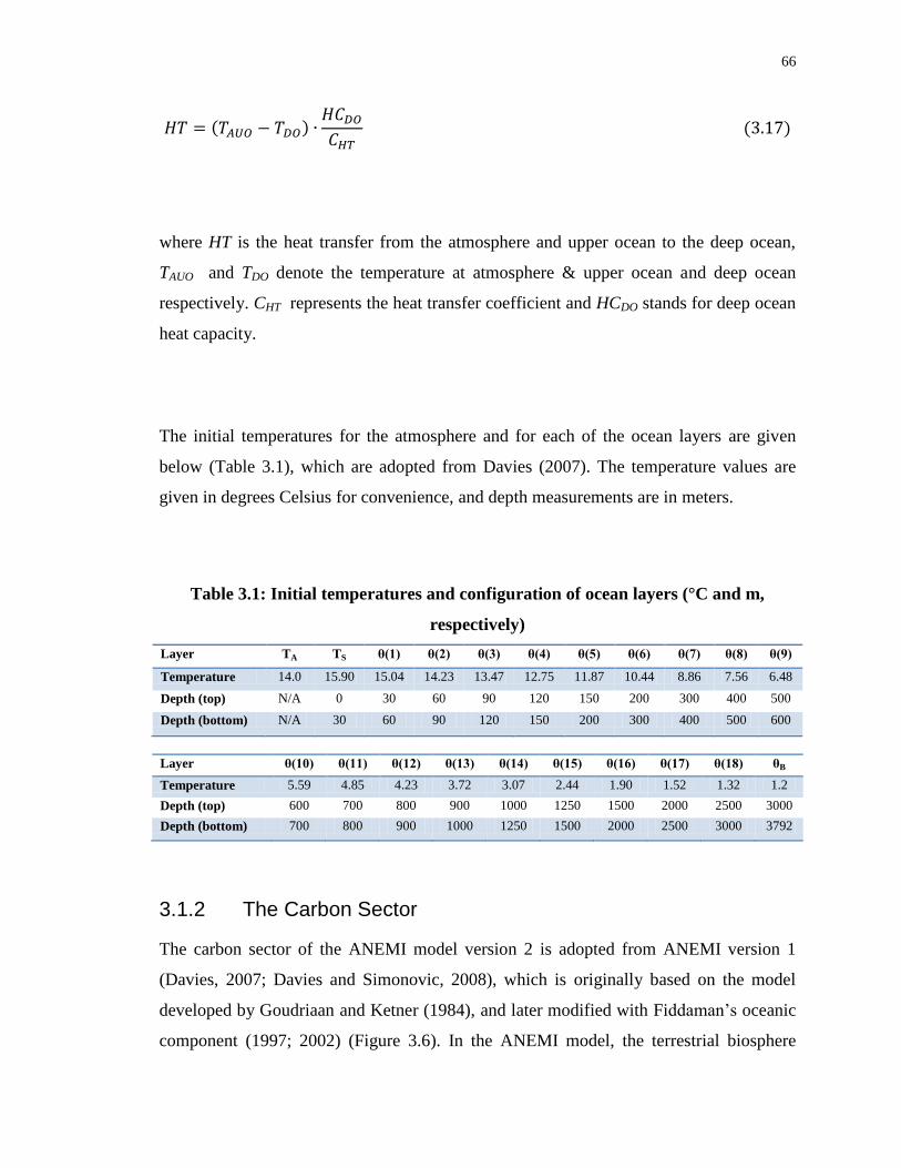
66

where HT is the heat transfer from the atmosphere and upper ocean to the deep ocean,

TAUO and TDO denote the temperature at atmosphere & upper ocean and deep ocean

respectively. CHT represents the heat transfer coefficient and HCDO stands for deep ocean

heat capacity.

The initial temperatures for the atmosphere and for each of the ocean layers are given

below (Table 3.1), which are adopted from Davies (2007). The temperature values are

given in degrees Celsius for convenience, and depth measurements are in meters.

Table 3.1: Initial temperatures and configuration of ocean layers (°C and m,

respectively)

Layer TA TS θ(1) θ(2) θ(3) θ(4) θ(5) θ(6) θ(7) θ(8) θ(9)

Temperature 14.0 15.90 15.04 14.23 13.47 12.75 11.87 10.44 8.86 7.56 6.48

Depth (top) N/A 0 30 60 90 120 150 200 300 400 500

Depth (bottom) N/A 30 60 90 120 150 200 300 400 500 600

Layer θ(10) θ(11) θ(12) θ(13) θ(14) θ(15) θ(16) θ(17) θ(18) θB

Temperature 5.59 4.85 4.23 3.72 3.07 2.44 1.90 1.52 1.32 1.2

Depth (top) 600 700 800 900 1000 1250 1500 2000 2500 3000

Depth (bottom) 700 800 900 1000 1250 1500 2000 2500 3000 3792

3.1.2 The Carbon Sector

The carbon sector of the ANEMI model version 2 is adopted from ANEMI version 1

(Davies, 2007; Davies and Simonovic, 2008), which is originally based on the model

developed by Goudriaan and Ketner (1984), and later modified with Fiddaman‘s oceanic

component (1997; 2002) (Figure 3.6). In the ANEMI model, the terrestrial biosphere

67

consists of six biomes: 1) tropical forests, 2) temperate (or boreal) forests, 3) grasslands,

4) agricultural lands, 5) deserts/ and tundra, and 6) settled areas. Living biomass is

divided into leaves, branches, stems and roots. Dead biomass is divided into three soil-

carbon pools, litter, humus, and charcoal or decay-resistant humus (Davies and

Simonovic, 2008). In this model, the carbon circulates through the atmosphere, the

terrestrial biosphere, and the oceans.

Figure 3.6: Model structure of the ANEMI model version 2 carbon sector

Carbon dioxide is easily dissolved in seawater, and its solubility is temperature

dependent. Colder water can dissolve more CO2, while higher water temperature reduces

the solubility according to Henry‘s Law. Henry‘s Law states that CO2 is in equilibrium

between air and water at 25 0C when approximately 1/50 of the gas is in the air and the

remaining gas is dissolved in the water. If 50 units of gas are added to the air 49 units will

thus be dissolved into the water.

Biomass

Litter

Humus

StableHumus andCharcoal

Carbon in Atmosphere

NPP

Litterfall

Decay tohumus

Decayfromlitter

Decayfrom

humus

Carbonization

Humification

Decayfrom

charcoal

Unburnt wood

Biomass tocharcoal

Litter tocharcoal

BurntBiomass

Burnt litter

Internal humusflows

Internalcharcoal flows

CumulativeEmissionsFossil fuel

burning

Carbon inMixed Layer

Carbon inDeepOcean

Diffusion flux

Concentration

Equilibrium carbon in mixed layer

Mixing time

Flux atmsphereto ocean

Turn On humanland use

Atmospheric CO2concentration

Biome area

Carbonemissions

Turn on humanemissions

Decay ofroots

New industrialcarbon emissions

Temperature effecton solubility

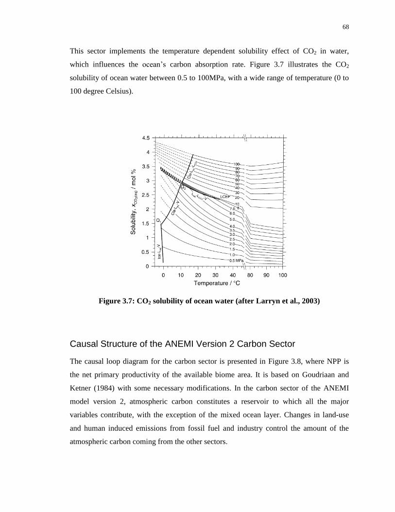
68

This sector implements the temperature dependent solubility effect of CO2 in water,

which influences the ocean‘s carbon absorption rate. Figure 3.7 illustrates the CO2

solubility of ocean water between 0.5 to 100MPa, with a wide range of temperature (0 to

100 degree Celsius).

Figure 3.7: CO2 solubility of ocean water (after Larryn et al., 2003)

Causal Structure of the ANEMI Version 2 Carbon Sector

The causal loop diagram for the carbon sector is presented in Figure 3.8, where NPP is

the net primary productivity of the available biome area. It is based on Goudriaan and

Ketner (1984) with some necessary modifications. In the carbon sector of the ANEMI

model version 2, atmospheric carbon constitutes a reservoir to which all the major

variables contribute, with the exception of the mixed ocean layer. Changes in land-use

and human induced emissions from fossil fuel and industry control the amount of the

atmospheric carbon coming from the other sectors.

69

Biomass is converted to litter when leaves fall from the plants. A fraction of the litter

returns back to the atmosphere by root decay and forest burning. The remaining litter is

converted to stable humus and charcoal. Humus both stores and releases carbon. It

collects and stores carbon from the biomass and litter (from forest burning and unburnt

wood), and it releases carbon into the atmosphere through decay and the carbonization

process.

Figure 3.8: Causal loop diagram of the ANEMI version 2 carbon sector

Mathematical Description of the ANEMI Version 2 Carbon Sector

This section provides all the equations of the carbon cycle, and their associated

parameters, beginning with the atmosphere. The mathematical formulation of the carbon

sector of ANEMI model version 2 is adopted from Davies (2007) with minor

adjustments, where equations for the terrestrial biosphere and the atmosphere are based

Energy-EconomySector

70

on Goudriaan and Ketner (1984), and the oceanic carbon absorption rate is based on

Fiddaman (1997; 2002).

Carbon is incorporated in several different stocks and expressed as follows: accumulation

of carbon in the atmosphere (Equation 3.18), accumulation of biomass (Equation 3.21),

litter stock (Equation 3.22), humus stock (Equation 3.23), charcoal stock (Equation 3.24),

mixed-layer oceanic carbon stock (Equation 3.25), and deep oceans carbon stock

(Equation 3.26). For further details see Davies and Simonovic (2008).

The accumulation of carbon in the atmosphere is expressed as,

where NPP is the net primary productivity. DB, DL, DH, and DK are the transfer of

decomposing organic matter from the terrestrial biomass, litter, humus, and charcoal to

the atmosphere, respectively. BB and BL are the biomass burning from land-use and land-

use change, E is the industrial emissions, and FO is the carbon absorption by the oceans.

However, in the ANEMI model version 2, industrial emission is calculated in more

comprehensive way compared to ANEMI version 1 (see section 3.1.3).

Net primary productivity can be computed as,

71

where NPPjk refers to the biome type (j) and the biomass component (k), pjk is the fraction

of biomass partitioned to component k of biome j. pjk, along with other parameters of the

carbon flows through the terrestrial biosphere, are given in Table 3.2, which has been

reproduced from Table 3.1 of Goudriaan and Ketner (1984: 178).

The equation for the variable surface density of net primary productivity σ(NPPj), is,

Where β is the CO2-fertilization factor, s CA and CA0 are respectively the current and

initial carbon dioxide concentrations in the atmosphere. Values for σ(NPPj)0 are given in

Table 3.3 (after Davies, 2007).

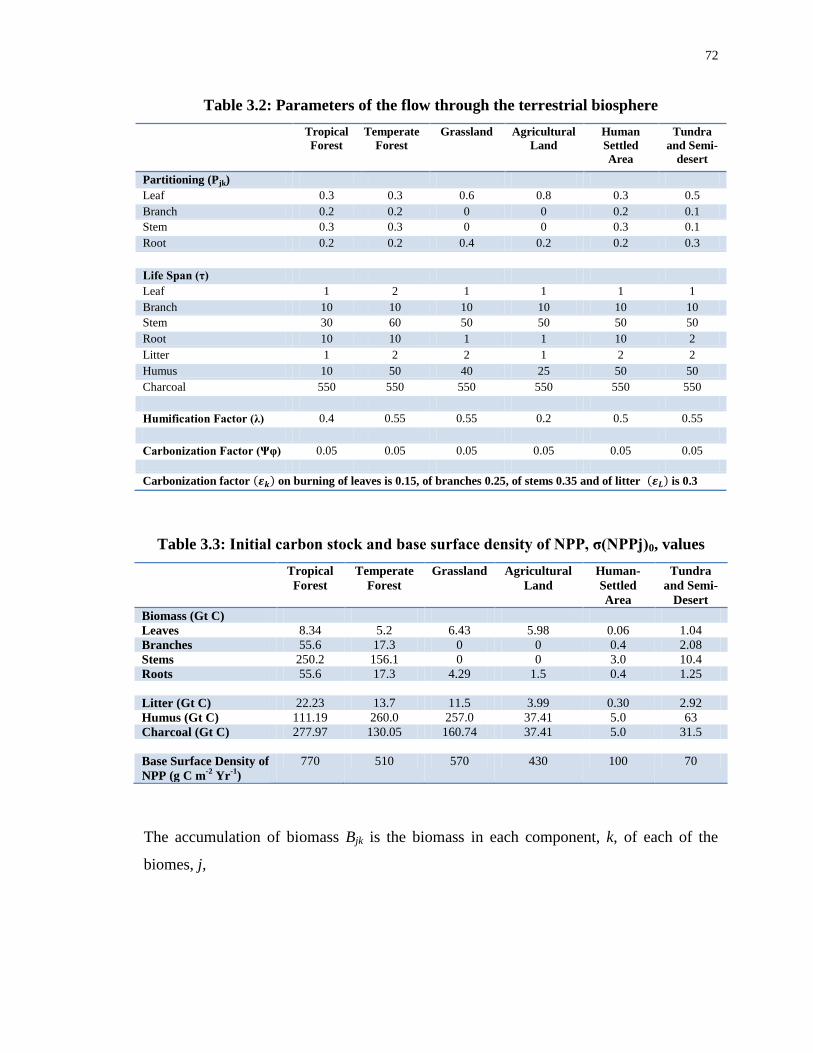
72

Table 3.2: Parameters of the flow through the terrestrial biosphere

Tropical

Forest

Temperate

Forest

Grassland Agricultural

Land

Human

Settled

Area

Tundra

and Semi-

desert

Partitioning (Pjk)

Leaf 0.3 0.3 0.6 0.8 0.3 0.5

Branch 0.2 0.2 0 0 0.2 0.1

Stem 0.3 0.3 0 0 0.3 0.1

Root 0.2 0.2 0.4 0.2 0.2 0.3

Life Span (τ)

Leaf 1 2 1 1 1 1

Branch 10 10 10 10 10 10

Stem 30 60 50 50 50 50

Root 10 10 1 1 10 2

Litter 1 2 2 1 2 2

Humus 10 50 40 25 50 50

Charcoal 550 550 550 550 550 550

Humification Factor (λ) 0.4 0.55 0.55 0.2 0.5 0.55

Carbonization Factor (Ψυ) 0.05 0.05 0.05 0.05 0.05 0.05

Carbonization factor on burning of leaves is 0.15, of branches 0.25, of stems 0.35 and of litter is 0.3

Table 3.3: Initial carbon stock and base surface density of NPP, σ(NPPj)0, values

Tropical

Forest

Temperate

Forest

Grassland Agricultural

Land

Human-

Settled

Area

Tundra

and Semi-

Desert

Biomass (Gt C)

Leaves 8.34 5.2 6.43 5.98 0.06 1.04

Branches 55.6 17.3 0 0 0.4 2.08

Stems 250.2 156.1 0 0 3.0 10.4

Roots 55.6 17.3 4.29 1.5 0.4 1.25

Litter (Gt C) 22.23 13.7 11.5 3.99 0.30 2.92

Humus (Gt C) 111.19 260.0 257.0 37.41 5.0 63

Charcoal (Gt C) 277.97 130.05 160.74 37.41 5.0 31.5

Base Surface Density of

NPP (g C m-2

Yr-1

)

770 510 570 430 100 70

The accumulation of biomass Bjk is the biomass in each component, k, of each of the

biomes, j,

73

where FLBjk is the amount of litter falling from the biomass to the litter layer, FHBjk is the

decay of biomass to humus, FKBjk is the burning of biomass, BBjk is the burning of

biomass from human land-use, and UBjk is the unburned remainder of biomass.

The equation of the litter stock Lj is,

where ΣFLB jk is the total litter fall, DLj is the flow of carbon from litter to the atmosphere,

FHLj is the decomposition of litter into humus, BLj is the carbon flow from litter to the

atmosphere, and FLKj is the carbon flow from litter directly to charcoal.

The humus stock Hj can be expresses as,

where ΣFHBjk is the decay of biomass to humus, FHLj is the decomposition of litter to

humus, FKHj is the decomposition of humus to charcoal, DHj is the decay of humus to the

74

atmosphere, ΣUBjk is the unburned remainder of biomass, and FHHj is an internal flow of

humus.

The mass of charcoal stock Kj has the following form,

where FKHj is the flow of carbon from humus to charcoal; DKj is the decay of charcoal,

ΣFKBjk is the burning of biomass, FKLj is the carbon flow from litter to charcoal, and FKKj

is an internal flow of charcoal from one biome to another. Initial values for each of the

terrestrial stocks are provided in Table 3.3, based on Table 3.2 of Goudriaan and Ketner

(1984: 178).

For the mixed-layer carbon stock (CML),

=

where FOA is the absorption of carbon dioxide by the mixed-layer from the atmosphere,

and DFO(0) is the diffusive flow of carbon dioxide to the deep ocean.

For the deep ocean carbon stock CO(h) in layer h is,

75

where DFO(h) is the diffusive flow of carbon from the layer above to the current layer h,

and DFO(h+1) is the diffusive flow to the layer below from the current layer. In this

model, the ocean is divided into ten layers of unequal depth, with each of the top five

layers having a thickness of 200 m, and the bottom five layers having a thickness of 560

m each.

3.1.3 The Energy-Economy Sector

The energy-economy sector of the ANEMI model version 2 describes the world‘s energy

resources, as well as how prices move to reflect the global demand and supply of energy.

It‘s an extension of the traditional (Solow) neoclassical growth model (see Appendix A).

The novel part of the model is the energy price is governing the allocation of energy

production across fossil fuels, hydro, nuclear, and alternative energy sources.

The model follows the common macroeconomic assumption that the global economy

consists of a representative household and a representative firm. The household displays

preferences over an aggregate consumption good, and it supplies labour services

inelastically to the firm each period. The firm takes labour, capital, and energy services as

inputs in a Cobb-Douglas production function (see Appendix A), and produces the final

good which is used for consumption and investment. Investment is determined by a

Solow rule where a fraction of output is invested into new capital each period. There is

no trade in the model.

76

‗Energy services‘ comprise a composite good that is aggregated from heat energy and

electric energy. Heat energy is produced from fossil fuels and alternative energy sources.

Electric energy is produced from fossil fuels, nuclear, and hydro power.

The production of output is negatively affected by climate damages. The global mean

temperature represents a negative impact to the economic system from industrial

emissions through climate damages.

The energy data for the global energy economy is from the U.S. Energy Information

Administration (EIA) and the World Bank‘s World Development Indicators (WDI).

Fossil fuel reserves, fossil fuel discoveries, the total energy produced from fossil fuel and

the total electricity produced from nuclear and hydro power data are respectively

collected from the EIA database (EIA, 2006). The WDI database

(http://databank.worldbank.org, last accessed August 2011) is used to collect data on the

production of electricity from fossil fuels.

One very important input into the model regards the future paths of oil and natural gas

extraction. The uncertainty associated with the size of undiscovered reserves in the Arctic

is but one factor. Another, perhaps greater uncertainty is the future development and

price of technology that may allow for extraction of resources considered unrecoverable

today. The U.S. Geological Survey estimates that there are about 3.4 trillion barrels of

heavy oil in the world; however, only 450 billion barrels are recoverable given today‘s

technology and price level. As a benchmark calibration, it is assumed that future

‗discoveries‘ will be around 1.3 trillion barrels. A similar assumption is made for natural

gas. The implicit assumption is that higher fossil fuel prices will motivate technological

progress and make extraction of heavy oil and shale gas economically viable.

77

Causal Structure of the ANEMI Version 2 Energy-Economy Sector

The causal structure diagram for the energy-economy sector is presented in Figure 3.9. In

the ANEMI model version 2, the energy-economy sector takes global mean temperature

and population as inputs. The climate damage relationship is from Nordaus (2000); it is

represented by a quadratic function in global mean temperature. Changes in population

levels and demographics impact the productive capacity of the economy, as the labour

input for the firm is assumed to be the working age share of the world population.

In this model, the available energy resources are primitives. The available fossil fuel

reserves and the technology available to produce nuclear, hydro, and alternative energy

are presumed. The output produced from the energy-economy sector includes industrial

emissions and the world‘s gross domestic product. Industrial emissions are calculated

from the burning of fossil fuels in producing energy services. The gross domestic product

is equal to final output, and depends on the world‘s capital stock, labour force, and

energy resources. It may be noted that in the model energy production is an intermediate

good.

Figure 3.9: Causal loop diagram of ANEMI energy-economy sector

78

Mathematical Description of the ANEMI Version 2 Energy-Economy Sector

This sub-section presents a detailed description of the variables and equations of the

energy-economy sector. It also presents the assumptions made about the representative

household, the representative firm, and the choices available to them, given the world‘s

energy resources.

The world‘s population is assumed to be represented by a stand-in household whose

preferences can be represented by the utility function

where is a generic consumption good. The household supplies labour, , inelastically to

the market. It is assumed that the household owns the world‘s capital stock and natural

resources. Thus, the consumer rents the capital to the firm, earning income , where is

the interest rate and is the aggregate capital stock in the economy. The consumer also

sells energy services to the firm, earning income , where E is the aggregate of energy

services, and is the price of aggregate energy services. Earning income from the

labour force , where is the wage rate.

Investment, , is assumed to follow a Sollow investment rule where a fraction s of output,

, is invested into new capital each period. Given prices, the household tries to maximize

the utility subject to its budget constraints. Each period the household‘s optimization

problem is:

79

The world‘s production of final output is represented by a stand-in firm that employs a

Cobb-Douglas production technology. The firm hires labour, capital, and energy services

from the stand-in household and produces generic consumption goods for it.

The aggregate production function is:

where , is total factor productivity (TFP), is the aggregate capital stock in the

economy, is the labour force, and is the Nordhaus damage coefficient. and are

the parameters of damage function. The damage coefficient is a function of , global

mean temperature. TFP is assumed to increase at a decreasing rate. TFP growth in 2005

is 1.6%, 0.9% in 2050, and 0.6% in 2100. The sum of the share parameters from the

aggregate production function, and , are assumed to decrease over time. This

assumption implies that the share of energy services in final output is decreasing. That is,

80

consistent improvements in technology reduce the energy intensity of the economy as a

whole.

The formulation used in this thesis assumed that there is a government in the model that

can implement carbon taxes on energy consumption. The government is exogenous to the

model, and tax revenues are transferred as a lump-sum to the household. We assume a set

of fuel specific taxes, , that depend on the emissions intensity of each fuel type i.

Finally, is the sum of tax revenues from carbon emissions. Then, is the

household‘s income from selling energy services to the firm net of taxes.

It is assumed that representative firms produce heat energy and electric energy from CES

production functions. Aggregate energy services, E, is modeled as a composite good

produced from heat energy and electric energy.

Electric energy is produced from fossil fuels, nuclear and hydro power. Here, nuclear and

hydro power are assumed policy variables, and are exogenous to the firm. For each

period the representative firm solves the following optimization problem:

subject to

given.

81

where

.

and

, for i=1,2,3.

That is, given the capital stocks for fossil fuels and the nuclear and hydro power

available, the representative firm chooses to minimize the

average total cost of electricity. Here, is a productivity term specific to electricity

production, is the fuel input used for fuel type in electricity production, is

the average total cost of electric energy, is the threshold value for electric energy,

is the price of electric energy and is the CES elasticity parameter (which implies

elasticity of substitution of .

The functions , for the fossil fuels, are decreasing in the fuel-to-capital ratio. Within a

given period this assumption implies diminishing returns, as capital is a fixed factor. The

parameters and are fixed. The parameters and are used to calibrate the relative

levels of fossil fuels in electricity production.

The structure for the production of heat energy is symmetric to the production of electric

energy. It is assumed that heat energy is produced from fossil fuels and alternative energy

sources. In each period, the representative firm solves the following optimization

problem:

82

subject to

where,

There is no capital in the heat energy sector. The capital for heat energy comprises part of

the aggregate capital for the economy. The firm chooses

to minimize the average total cost of heat energy. Here,

is a productivity term specific to heat energy production, is the input of fuel type

i for heat energy production, is the CES weight for fuel type i, is the average

total cost of heat energy, is the threshold value for heat energy, is the heat energy

service, is the price of heat energy services, and is the CES elasticity parameter.

and are assumed to grow linearly. Implicit productivity increases are reflected in

the respective assumptions of fossil fuel discoveries, the price function of alternative heat

energy, and the share parameters in the aggregate production function. Currently, and

are arbitrarily set equal to 0.5.

The fossil fuel price functions are increasing in the ratio of the reserve value at its base

year relative to its current value.

83

where subscripts i and t refer to the fossil fuel type and the year respectively. is the

fuel price, is the fuel specific carbon tax, is the price of fuel at the base year

(1980), is the current reserve level, , is the base year reserve level, and is

the new discovery value. and

are the extractions of fuel for electricity and heat

energy production respectively. is an elasticity parameter.

It is clear that the price of fossil fuel decreases when the current reserve value falls

relative to the base year. That is, the more fuel extracted the higher the price becomes.

New discoveries of fossil fuel reduce the price of fossil fuel, holding everything else

constant. The paths for new fossil fuel discoveries are prescribed. The elasticity

parameter for the fossil fuel price functions, , is set to -0.4. A lower value would make

fossil fuel prices more responsive to the depletion of fossil fuel reserves. The parameter

value and the functional form for the price functions are from the ANEMI version 1.2

energy-economy sector (Davies and Simonovic, 2009).

The price of alternative heat energy is represented by the function:

where is the price, and is the quantity of alternative fuel used in heat energy

production. and are parameters. It is assumed that they are decreasing, representing

decrease of the alternative fuel price over time.

84

The initial values for the parameters for the alternative energy price function, and ,

are assumed equal to 3 and 5 respectively. The parameters decrease linearly over time,

representing a decrease in the price of alternative energy over time as technology

improves. For the calibration we had a target of 3% alternative heat energy in 2005. The

energy demand side is derived from the aggregate production function.

For one period problem the capital and labour inputs are fixed. Demand for aggregate

energy services can be expressed as:

where is the representative firm‘s demand for aggregate energy services, is aggregate

capital, is the world‘s labour force, and is the price of aggregate energy services.

and are the share parameters from the aggregate production function.

Heat energy and electric energy are combined into aggregate energy services by a CES

function:

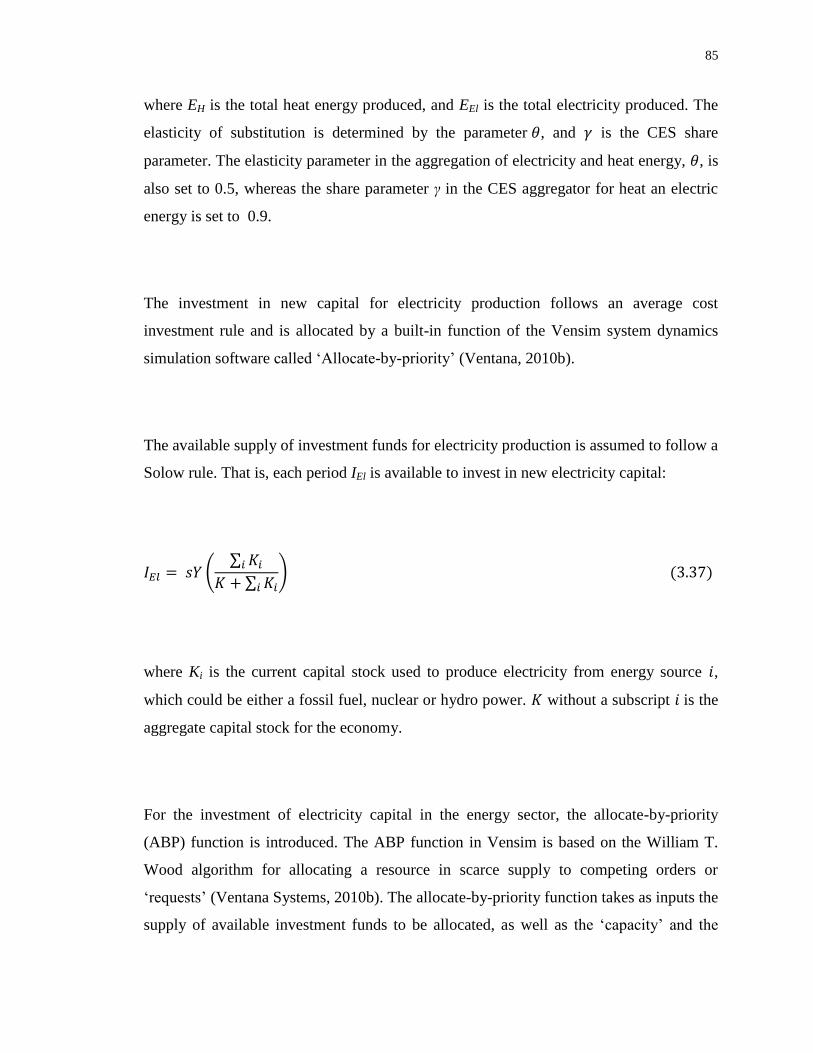
85

where EH is the total heat energy produced, and EEl is the total electricity produced. The

elasticity of substitution is determined by the parameter , and is the CES share

parameter. The elasticity parameter in the aggregation of electricity and heat energy, , is

also set to 0.5, whereas the share parameter γ in the CES aggregator for heat an electric

energy is set to 0.9.

The investment in new capital for electricity production follows an average cost

investment rule and is allocated by a built-in function of the Vensim system dynamics

simulation software called ‗Allocate-by-priority‘ (Ventana, 2010b).

The available supply of investment funds for electricity production is assumed to follow a

Solow rule. That is, each period IEl is available to invest in new electricity capital:

where Ki is the current capital stock used to produce electricity from energy source ,

which could be either a fossil fuel, nuclear or hydro power. without a subscript is the

aggregate capital stock for the economy.

For the investment of electricity capital in the energy sector, the allocate-by-priority

(ABP) function is introduced. The ABP function in Vensim is based on the William T.

Wood algorithm for allocating a resource in scarce supply to competing orders or

‗requests‘ (Ventana Systems, 2010b). The allocate-by-priority function takes as inputs the

supply of available investment funds to be allocated, as well as the ‗capacity‘ and the

86

‗priority‘ of each order, which respectively represent the size and competitiveness of the

orders.

The ABP function has a ‗width‘ parameter that determines how exclusively the available

investment funds will be allocated. The width-parameter can take any positive value. The

lower the value of the width, the more responsive the allocation to differences in order

priority will be. For example, if two orders have similar capacitates and priorities, then a

high width will produce a very even allocation. On the other hand, as the width parameter

decreases, the allocation of investment funds will be shifted towards the order with the

higher priority.

Given the fixed quantity of investment funds available inside a period, the market

allocation depends on (a) the size of the request, (b) the relative priority given to each

sector, and (c) the width parameter. After testing multiple approaches, we decided to set

the priorities for the sectors equal to each other, and only focus on the request dimension.

With this decision, we intended to simplify the calibration and to make the investment

function more transparent. More information about the ABP function in Vensim can be

found in the Vensim manual and the supporting documentation online

(http://www.vensim.com/allocp.html, last accessed August 2011).

The demand for new investment funds for each energy source of electricity production is

based on an average cost investment rule, where the allocation is determined by the ABP

function. Given a fixed priority across energy sources, the ‗request‘ function takes the

following form:

87

The request for new investment funds ( ) is a function of both ‗replacement capital‘

and the current capital share of the sector scaled by its relative average total cost. In each

period, a share of existing capital depreciates, and an assumption is made that all

sectors will ask for that capital to be replaced. The parameter is a weighting factor that

will reduce the request for replacement capital if the average total cost exceeds some

threshold value. The second term is the relative size of the current capital stock (Ki) for

energy source multiplied by its relative average cost. This implies that sectors with a

lower average cost will have higher requests. is the average total cost of

electricity, and is the average total cost of energy source .

The value of φ is set to 0.5; this means that if the condition is true, then the request for

replacement capital is only half of the depreciated capital. With this parameter, the idea is

to improve the adjustment process of the capital stock in electricity production from

fossil fuels in response to average cost changes.

Note that as the path for nuclear and hydro power is given exogenously, the capital stock

used in production of nuclear and hydro power is also prescribed. The amount needed for

new capital for nuclear and hydro power is first subtracted from the total amount

available for investment into electricity capital; what is left over is allocated to the fossil

fuel capital stocks using the ABP function.

In the ANEMI model, the consumed portion of fossil fuel energy resources is converted

into the respective carbon emissions mass. This approach dovetails with the IPCC‘s

recommendations for calculating tier one emissions (IPCC, 2006: Vol. 2, Ch. 2, Pg.

2.11).

88

Carbon emissions are calculated as follows:

Coal:

On average, the energy content of coal is 21.213 GJ tcoal-1

; this means that the combustion

of 1 ton of coal releases:

1. 0.518 tons of carbon, for an emission factor of 0.518 tC tcoal -1

(EIA, 2008); or

2. 0.541 tons of carbon, for an emission factor of 0.541 tC tcoal -1

(IPCC, 2008 [using

26 tC TJ-1

, 98% combustion].

where is the emission for the coal, is the combustion amount out of 1 unit,

is the emission factor of coal. represents the amount of coal depleted from

the reserve, i.e. the amount used in energy production.

Oil:

On average, the energy content of oil is 6205 MJ bbl-1

; this means that the combustion of

1 barrel of crude oil releases;

1. 0.119 tons of carbon, for an emission factor of 0.119 tC bbl-1

(EIA, 2008); or

2. 0.125 tons of carbon, for an emission factor of 0.125 tC bbl-1

(IPCC, 2008) [using

20.5 tC TJ-1

, 99% combustion].

89

where is the emission for the oil, is the combustion amount out of 1 unit,

is the emission factor of oil. represents the amount of oil depleted from the

reserve or used in energy production.

Natural gas:

On average, the energy content of natural gas is 38.264 MJ m-3

, and this means that the

combustion of 1 m3 of natural gas releases

1. 5.246 x 10-4 tons of carbon, for an emission factor of 0.0005246 tC m-3

(EIA,

2008); or

2. 5.796 x 10-4 tons of carbon, for an emission factor of 0.0005796 tC m-3

(IPCC,

2008) [using 15.3 tC TJ-1

, 99% combustion].

where is the emission for the Natural Gas, is the combustion amount out

of 1 unit, is the emission factor of Natural Gas. represents the

amount of natural gas depleted from the reserve or used in energy production.

The ANEMI model version 2 used the first-listed emissions factors for each of the three

fossil fuels. These factors give the closest correspondence to historical emissions values,

as we will show in the next section. The combustion factor states that the combustion

process uses 99% of the fuel, and this also corresponds to the data.

90

For the sake of simplicity, it is assumed that future fossil fuel discoveries are known at

the beginning of the time horizon. The sum of the total discoveries is added to the initial

reserve value in the base year. This assumption makes global fossil fuel price movement

smooth, which is helpful as the price paths are used as inputs to the energy-economy

sector of the Canada regional model.

Table 3.4 lists the initial reserve values for the base year. The first column shows the

initial reserve value used in the baseline model. This value is calculated as the sum of

observed 1980 reserves, observed discoveries from 1980-2005 of EIA (2006), and

assumed discoveries after 2006.

Table 3.4: Initial fossil fuel reserve (in trillion GJ)

1980

Assumed Initial

Reserves

1980 Reserves

(EIA)

1980-2005

Discoveries (EIA)

2006 -

Assumed

Discoveries

Coal 20 20 - -

Oil 21 3.9 6.8 10.3

Natural Gas 18 2.7 5.7 9.6

Numerical Solution of the ANEMI Version 2 Energy-Economy Sector

The ANEMI model version 2 was developed using Vensim system dynamics simulation

software (Ventana Systems, 2010a). The model structure allows for the analyses of

numerous feedback relationships within each sector and between different sectors.

However, the energy-economy sector presented above involves optimization of problems

in Equations (3.53), (3.56) and (3.57). In macroeconomics, the most common way to

solve these optimization problems computationally is by employing various iterative

nonlinear optimization algorithms.

91

Vensim‘s scope for optimization is limited. As a consequence, the energy-economy

sector employs a MATLAB software optimization package subroutine. In each

simulation time step, Vensim sends information to MATLAB, which solves the one-

period optimization problem for the energy-economy. More specifically, at each time-

step Vensim sends MATLAB the global mean temperature, the capital stocks of energy

production, and the population data. MATLAB is then used to solve a non-linear system

of equations, a system that represents the optimal solution to the one-period optimization

problem in the energy-economy sector. The solution to that problem is the production

allocation, the optimal energy use across energy sources in production. The production

allocation is then sent back to the Vensim simulation model. (For further details, see

Chapter 7). Based on the energy consumption it calculates, Vensim can run the next time-

step, and calculate emissions. These emissions are in turn used to calculate global mean

temperature. This last value is then used by other sectors of the ANEMI model.

The current modelling approach allows for a market clearing mechanism in the energy-

economy, where energy prices move to equate supply and demand. The main drawback

of this approach is the increase in the model‘s computation time.

3.1.4 The Food Production Sector

With respect to the food production sector, the fundamental assumption is that the global

amount of food that can be produced each year is limited. It is proven that the proper

allocation of physical resources (water, fertilizer, suitable land, etc.) can enhance food

production. However, these resources are not abundant. One can argue that the

technological innovations may lead to a very high yield within the same agricultural area.

But it has become evident that there are decreasing returns to technology‘s ability to

increase land yield by diverting the input of other limited resources into the agriculture

sector (Meadows et al., 1974; Gilbert et al., 1991).

92

Arable, cultivated land is at present the most important source of food production for

human consumption. But it is not the only one. Other sources of food production include

the oceans and the world‘s grazing lands. However, the analyses of FAO data

(AQUASTAT, 2010) established that only 7.4% of the total amount of food produced

comes from animal product (Figure 3.10).

The current and potential food output from both fisheries and grazing land is thus very

small compared to the food output from the cultivation of arable land (Meadows et al.,

1992). Hence we decided not to take into account the food obtained from oceans and

grazing lands in the ANEMI model version 2. The world‘s grazing lands, for example,

currently cover 3.6 billion hectares, an area somewhat larger than the potentially arable

land of 3.2 billion hectares. The average carrying capacity of the world‘s grazing lands is

roughly 1 animal unit per 20 hectares, where 1 animal unit is equivalent to the production

of 100 kilograms of meat per year (Meadows et al., 1974). If it is assumed that 7

kilograms of vegetable crops are needed to produce 1 kilogram of meat, this yields the

amount of 35 vegetable-equivalent kilograms per hectare per year. Thus the vegetable-

equivalent food yield from grazing lands is low in comparison to the traditional yield of

600 vegetable-equivalent kilograms per hectare-year that can typically be obtained from

arable land without the use of modern agricultural inputs. The grazing land yield is only

about 2 percent of the world average cultivated land yield of around 2,000 vegetable-

equivalent kilograms per hectare-year. In short, the food output from grazing land is of

relatively lower importance (Meadows et al., 1974).

93

Figure 3.10: Yearly food production (billion veg-eq-kg)

The food production sector of the ANEMI model version 2 (Figure 3.11) is based on the

WORLD3 model (Meadows et al., 1974). In this latter model, the capital investments in

agriculture can increase total food production in two ways: (a) by increasing the stock of

arable land through land development, and (b) by increasing land yield through the

application of modern agricultural inputs.

The agriculture sector also distinguishes between two phenomena that can reduce overall

food production. The first one is ‗land erosion‘: an irreversible centuries-long process

that physically removes land from production. The rate at which land erodes can be large

or small, depending on the human actions taken to control the erosion rate, but it is

assumed that the direction of land movement cannot be changed. The erosion rate could

be zero, but it will never become negative. The second phenomenon that can reduce land

yield and thus food production is ‗lower land fertility‘, that is, by a reduction in the

humus and nutrient content of the soil. This is a reversible process, since the degradation

of the land‘s fertility occurs only when insufficient resources are allocated to the

1000

1500

2000

2500

3000

3500

4000

1960 1970 1980 1990 2000 2010

Fo

od

Pro

du

ctio

n (

Bil

lio

n.

veg

-eq

-kg

)

Time

Yearly Food Production

Total food production

Food production (without animal product)

94

enhancement of the natural soil‘s regeneration mechanisms. In lower land fertility, the

soil‘s regenerative forces do not manage to keep up with the ongoing forces of

degradation.

In the ANEMI model version 2 all types of arable land are included in a single stock, so

the model reflects in a single quantity, the aggregate of all different lands with the

varying cultivation characteristics.

Figure 3.11: Model structure of the ANEMI version 2 food production sector

Technological change affects relationships in the agriculture sector in a variety of ways.

Some of the effects of advances in technological capability are included endogenously in

the food production sector. For instance, it is assumed that the allocation of more

investment to increasing land yield will have roughly the same success in the total global

agricultural system. Such an assumption implies that the regional variations posed by

different soils, climates, and traditional cultivation procedures will be eliminated by the

Emissionindex Land fertility

degradation rate

Land FertilityLand fertilityregeneration

Land fertilitydegradation

Inherent landfertility

Land fertilityregain time

Fraction of inputsallocated for land

maintenance

Food ratio

Food storageperception delay

Food percapita

Food

Processingloss

Land fractionharvested

Land yield

PerceivedFood RatioChange percived

food ratio

Agricultural inputper hectare

Land yieldmultiplier cap

Total ErodabeLand Land erosion

rate

Average life ofland

Land life multiplierfrom land yield1

Net arableland

Land life multiplierfrom land yield

Food productionper hectare

Impacted agriculturalarea for sea level rise (ha)

95

advancement of technology. In the same manner it is also assumed that the investment in

land maintenance, regeneration of land fertility, will always succeed.

Causal Structure of the ANEMI Version 2 Food Production Sector

The causal loop diagram for the food production sector is presented in Figure 3.12. It is

based on the WORLD3 model of Meadows et al. (1974). This figure represents a

simplified representation of the causal loop structure of the food production sector. The

complex land yield is obtained from the variables of land fertility, water-stress, and

capital investment. All of these variables are connected with positive polarity. The total

amount of food produced depends on such factors as land yield, availability of the

agricultural land, availability of the water for irrigation, and so on. In this diagram, the

food ratio works like a thermostat, by which extra investment is pumped in the food

production sector, when the ratio is below the threshold level. The extra investment is

used to improve land fertility, while technological development is used to enhance the

food production by increasing the land yield. Unplanned agricultural activity increases

the land erosion and decreases the land fertility. The forces of degradation are controlled

by a decrease in such activity.

The two most essential parameters of this sector are those of water-stress and arable land.

These come from the other sectors of the ANEMI model version 2. Population, which is

the product of the population sector, is used in the computation of the per capita food

production to assess the requirements for further investment.

96

Figure 3.12: Causal loop diagram of the ANEMI version 2 food production sector

Mathematical Description of the ANEMI Version 2 Food Production Sector

The important equations of the food production sector, and the values of their associated

parameters, are provided in this section. The food production sector description is based

on the work of Meadows et al. (1974).

The total annual food production is assumed to be the function of cultivated land and land

yield. It is assumed that there will not be any shortage of labour force. Hence labour force

is not included in this calculation. Indeed technological improvement means that labour

force requirements will steadily decrease over time. Thus the food output is calculated

simply as the output per hectare of harvested land times the total cultivated land area.

Energy-Economy Sector

Population Sector

Water Quality Sector

97

where is the amount of food production, is the land yield. The net arable land, land

fraction under harvesting, and processing loss are denoted by , and respectively.

Here, the processing loss is assumed as 10%.

The land yield Ly is the average total weight of crop production on a hectare of land per

year. In the ANEMI model version 2 land yield is partly computed by land fertility,

defined as the weight of crop that land will produce using only traditional inputs such as

human or animal energy and natural fertilizers, such as manure. The land yield, Ly, can be

increased significantly above the land fertility by the use of modern agricultural inputs.

where is the land yield factor, is the land fertiality, and is the land yield

multiplier from capital. Availability of water resources is a vital component of the land

yield, therefore Equation (3.68) also introduces water-stress to land yield factor ( ).

The land fertility ( ) is the average ability of one hectare of net arable land ( ) to

produce crops without the use of modern agricultural input. The fertility of the land is a

complex function of the organic and inorganic content of the soil, the climate, and the

incident solar radiation. Any process that interferes with soil chemistry, or the water

holding capacity of the soil, is likely to change the soil fertility. There are many such

processes, some with positive influence tending to regenerate soil fertility and some

tending to degrade it. In a simplified way the land fertility can be defined as:

98

where and stand for land fertility regeneration and land fertility degradation,

respectively.

The calculation of net arable land combines different inputs, including impacted

agricultural land due to sea-level rise. It represents the net cultivated area that is

dedicated directly to human food production. Therefore, it excludes the land area used for

the production of fodder and animal crop ( ), and can be expressed as:

where and respectively represent arable land and net erodible land. An obstacle

to land conversion is defined as and impacted agricultural land is denoted as .

3.1.5 The Land-Use Sector

Land-use change can be considered one of the factors contributing to the increase in CO2

concentration in the atmosphere. It therefore plays a key role in determining the

atmospheric level of carbon dioxide over long periods of time. It is estimated that an

added extra 1.6 ± 0.8 Gt C/year was released in the atmosphere in the 1990s due to

conversion of forests to agricultural land (Watson et al., 2000; Davies, 2007).

Anthropogenic greenhouse emissions contributed 6.7 Gt C (Marland et al, 2008) in 2000.

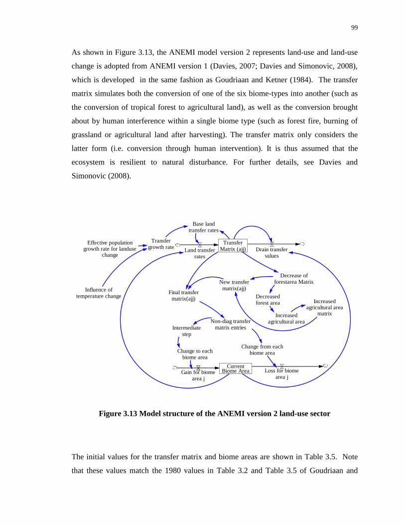
99

As shown in Figure 3.13, the ANEMI model version 2 represents land-use and land-use

change is adopted from ANEMI version 1 (Davies, 2007; Davies and Simonovic, 2008),

which is developed in the same fashion as Goudriaan and Ketner (1984). The transfer

matrix simulates both the conversion of one of the six biome-types into another (such as

the conversion of tropical forest to agricultural land), as well as the conversion brought

about by human interference within a single biome type (such as forest fire, burning of

grassland or agricultural land after harvesting). The transfer matrix only considers the

latter form (i.e. conversion through human intervention). It is thus assumed that the

ecosystem is resilient to natural disturbance. For further details, see Davies and

Simonovic (2008).

Figure 3.13 Model structure of the ANEMI version 2 land-use sector

The initial values for the transfer matrix and biome areas are shown in Table 3.5. Note

that these values match the 1980 values in Table 3.2 and Table 3.5 of Goudriaan and

TransferMatrix (ajj)Land transfer

rates

CurrentBiome Area

Non-diag transfermatrix entries

Change from eachbiome area

Intermediatestep

Change to eachbiome area

Transfergrowth rate

Base landtransfer rates

Drain transfervalues

Final transfermatrix(ajj)

New transfermatrix(ajj)

Decreasedforest area

Increasedagricultural area

Increasedagricultural area

matrix

Decrease offorestarea Matrix

Influence oftemperature change

Effective populationgrowth rate for landuse

change

Gain for biomearea j

Loss for biomearea j

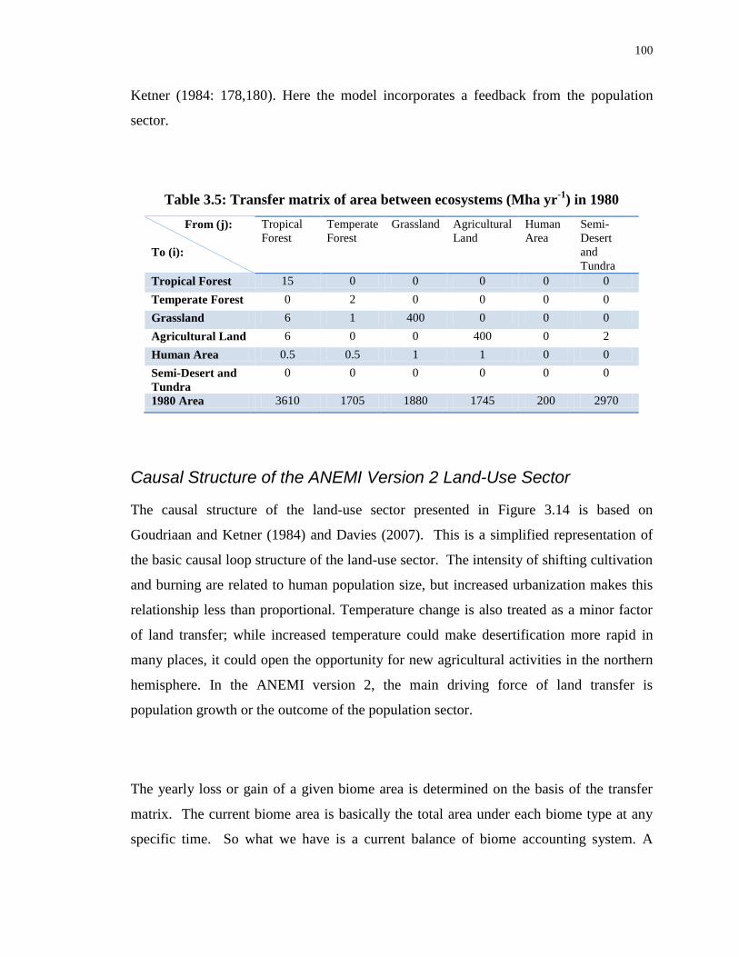
100

Ketner (1984: 178,180). Here the model incorporates a feedback from the population

sector.

Table 3.5: Transfer matrix of area between ecosystems (Mha yr-1

) in 1980

From (j):

To (i):

Tropical

Forest

Temperate

Forest

Grassland Agricultural

Land

Human

Area

Semi-

Desert

and

Tundra

Tropical Forest 15 0 0 0 0 0

Temperate Forest 0 2 0 0 0 0

Grassland 6 1 400 0 0 0

Agricultural Land 6 0 0 400 0 2

Human Area 0.5 0.5 1 1 0 0

Semi-Desert and

Tundra

0 0 0 0 0 0

1980 Area 3610 1705 1880 1745 200 2970

Causal Structure of the ANEMI Version 2 Land-Use Sector

The causal structure of the land-use sector presented in Figure 3.14 is based on

Goudriaan and Ketner (1984) and Davies (2007). This is a simplified representation of

the basic causal loop structure of the land-use sector. The intensity of shifting cultivation

and burning are related to human population size, but increased urbanization makes this

relationship less than proportional. Temperature change is also treated as a minor factor

of land transfer; while increased temperature could make desertification more rapid in

many places, it could open the opportunity for new agricultural activities in the northern

hemisphere. In the ANEMI version 2, the main driving force of land transfer is

population growth or the outcome of the population sector.

The yearly loss or gain of a given biome area is determined on the basis of the transfer

matrix. The current biome area is basically the total area under each biome type at any

specific time. So what we have is a current balance of biome accounting system. A

101

current biome area thus serves as a checking mechanism for unrealistic land transfer;

when a biome type reaches almost zero value, it completely converts to another.

Figure 3.14: Causal loop diagram of the ANEMI version 2 land-use sector

Mathematical Description of the ANEMI Version 2 Land-Use Sector

The land-use sector is represented by a very simple model structure. As indicated before,

the land transfer matrix (provided by Goudriaan and Ketner, 1984) is only influenced by

population growth. Temperature change is of minor impact.

It is assumed that the land transfer rate outside the diagonal direction of the transfer

matrix (see Table 3.5) is proportional to the population growth rate, while burning and

shifting cultivation (represented by the diagonal direction) grow with the square root of

the ‗population growth rate‘. Therefore, the land transfer rate can be expressed as:

102

where is the land transfer rate in non-diagonal direction, is the

transfer matrix, and denotes population growth rate.

In case of land transfer along diagonal direction, the transfer rate ( ) can be

describes as:

The transfer matrix works as a reservoir where inflow is land transfer rate and outflow is

drain transfer value ( . The drain transfer value is used in the model to avoid any

negative term. The following equation represents the generic form of the ‗transfer matrix‘

calculation. It can be used for both diagonal and non-diagonal matrix entities.

The area Aj of ecosystem j changes as:

where is the area of ecosystem j, is the rate of transition of area from ecosystem j

to ecosystem i.

103

3.1.6 The Population Sector

Two basic dynamics of the society-biosphere-climate-economy-energy system of the

Earth and biosphere are exhibited in a) the tendency in all human populations towards

exponential growth, and b) the long delay in the adaptive response of a population to

changing external conditions (Meadows et al., 1974). The actual rate of growth, the

nature of the adaptive response, and the length of delay all vary, depending on many

different factors in the total system.

When any biological population grows, the pattern of growth over time tends to be

exponential. In the twentieth century, rapid exponential growth has been exhibited not

only by the global human population but by nearly every national and regional population

as well (Meadows et al., 1974). The total increase in the global population during any

time period is determined at least partially by the size of the population of reproductive

age in that time period. For the global population, migration is not a factor, as there is no

consideration of spatial distribution of the population.

There is often significant delay in demographic responses to new external conditions

brought about by changes in the birth and death rates. The two major sources of the delay

are the age structure of the population and the inherent slowness of social change. It takes

at least 15 years for a newborn child to mature and become a parent (Figure 3.15). There

is a delay of more than 50 years before the child reaches the age of highest probability of

death. The long delays inherent in the biological processes of maturation and aging give

every human population a strong momentum, the tendency to keep following the same

dynamic behaviour that it has followed in the past (Meadows et al., 1974). Because of

the momentum, a population that has been growing rapidly will continue to grow for

decades, even after fertility has fallen to the equivalent of two surviving children per

married couple. Similarly, a population that has experienced a fertility rate that is lower

104

than the replacement level may continue to decrease in size for some time after the

fertility rate has again risen to the replacement level.

Figure 3.15: Model structure of the ANEMI version 2 population sector

The population sector includes a four-level population model, which means the

population is divided into 4 age groups (0 to 14 yr; 15 to 44yr; 45 to 64yr; and 65 to 65

plus). For initial stocks values, the UN data (DESA, 2011) of 1980 is used.

Causal Structure of the ANEMI Version 2 Population Sector

The population sector of the ANEMI model version 2 is based on the WORLD3

population model (Meadows et al., 1974). It represents continuous dynamic interactions

among the human population, climate and global resources (Figure 3.16). The population

sector model contains numerous feedback loops representing demographic and

technological-economic means of achieving a favourable balance between the population

size and the supply of resources. In this model crowding, pollution, availability of food,

Population:age 0 to 14

Population:age 15 to 44

Population:age 45 to 64

Population:age 65 plus

births Matured 14 to15

Matured 44 to45

Matured 64 to65

Deaths65 plus

Deaths 45 to64

Deaths 15 to44

Deaths 0 to 14

Deaths

Reproductivelifetime

Mortality 45to 64 Mortality 65

plus

Mortality 15to 44

Mortality 0 to14

Total fertility

Population

Birth rate<Life expectancy>

Total temperaturerelated death 65+

Populationgrowth rate

Total temperaturerelated death 0-14

105

and household income affect average life expectancy. Life expectancy and extreme

temperature determine the population death rate. Fertility is determined by a number of

factors, including fertility control effectiveness, capital allocation, and desired family

size. Birth and death rates are the only two direct variables used in the population

computation.

Figure 3.16: Causal loop structure of the ANEMI version 2 population sector

Mathematical Description of the ANEMI Version 2 Population Sector

Many factors affect the population‘s average level of health or life expectancy, and it is

by no means easy to assess the role of each particular factor or how each one interacts

with the others. Sometimes one variable of interest appears to depend on a number of

others, and in such cases one can use statistical interface techniques to find out the

relative importance of the variables in question. In the case of life expectancy, Kusukawa

(1967) carried out just such a statistical analysis. Here, however, the empirical

Energy- EconomySector

Carbon Sector

Food Production Sector

Population

Deaths

Lifeexpectancy

Pollution

Crowding

Food percapita

Births

Fertility

Fertility controleffectiveness

Desired totalfertility

Maximum totalfertility

Need for fertilitycontrol

Family planningservice per capita

GDP

Foodproduction

water stress

extremetemperature

Water QualitySector

Climate Sector

106

relationship between food per capita and life expectancy is adopted from both Meadows

et al. (1974) and Keyfitz and Flieger (1971).

Four factors: (i) food, (ii) health services, (iii) crowding, and (iv) pollution are

incorporated in the equation for life expectancy as modifiers, or multipliers, of a ‗normal‘

life expectancy. The normal life expectancy can be set at any arbitrary value as long as

the four multipliers are all defined properly with respect to that value.

where LE is the life expectancy, LEN is the life expectancy normal, and LMF is the lifetime

multiplier from food. Lifetime multiplier from health service, persistent pollution, and

crowding are respectively represented as LMHS, LMP, and LMC.

In the population sector the number of deaths per year is expressed as the total

number of people of a specific age group multiplied by the mortality of

the same group.

where mortality is a function of life expectancy. This functional relationship is expressed

in Meadows et al. (1974, page 170-172) as:

107

The thermal stress related mortality should increase due to the climate change. It has

been established that 16 to 30 degree Celsius is the comfortable temperature zone. A 1

percent increase in the death rate could happen for 1 degree drop in temperature below 16

degree Celsius. On the other hand a 1.4 percent increase in the death rate may be

experienced per degree temperature rise above 30 degree Celsius (Martens, 1998). As

children and the elderly (people above 65 years of age) are mainly vulnerable to extreme

climate, so temperature related death is incorporated in the ANEMI model version 2 for

two age categories (0-14 and 65 plus). The Equation (3.75) therefore changes as follows:

The Equation (3.51) is still valid for the population between 15 to 64 years of age. The

number of births per year is calculated from (i) a purely demographic factor, (ii)

from the number of fertile women in the population (half of the total population between

the 15 to 44 age group), and (iii) from a socio-economic factor, the average number of

births per women per year.

where is the total fertility, is the reproductive lifetime of 30 years, and

is the total population between age 15 and 44.

108

Total fertility is computed from the maximum total fertility , desired total

fertility and fertility control effectiveness :

3.1.7 The Water Resources Sectors

The representation of global water resources in the ANEMI model version 2 includes

hydrologic cycle, water demand, and water quality sectors. Global hydrologic cycle and

water demand sectors can be found in many models: for example, WaterGAP2 (Alcamo

et al., 2003a), Water balance model (Vörösmarty, 2002b), Macro-PDM (Arnel, 1999a)

and etc. Simonovic (2002b) enhanced the existing WORLD3 (Medows et al., 1992) by

adding these water sectors. But despite such improvements, the water sectors of such

models are not dynamic in nature. For the first time, Davies and Simonovic (2008)

successfully introduced a detailed water resources component in the ANEMI model

version 1.1. The ANEMI model version 2 extends the work of Davies and Simonovic

(2009; 2010; 2011), and attempts to capture the dynamics of global water resources with

respect to both quality and quantity of water.

3.1.7.1 Hydrologic Cycle Sector

Water is the only natural resource that exists in three forms: liquid, solid (snow, ice) and

gas (clouds). Unlike most natural resources, it is renewable. Water reservoirs in the

global hydrologic cycle include the oceans, the land surface, groundwater, ice sheets, and

the atmosphere. They can thus be separated into marine and terrestrial components

(Chahine, 1992). Through the processes of evaporation and evapotranspiration,

advection, precipitation, snow and ice melting, percolation and base flow from aquifers,

and surface runoff to the oceans (Chahine, 1992; Gleick, 2000b; Shiklomanov, 2000), the

109

water is transferred from one reservoir/stock to another and thus hydrological cycle

continues.

The hydrologic cycle has no specific beginning or ending. Rather, liquid water from the

Earth‘s surface, particularly the oceans, is evaporated into a gaseous form and enters the

atmosphere as water vapour (clouds). The atmospheric moisture is eventually returned to

the Earth‘s surface in the form of rain or snow. The liquid fresh water moves over the

land surface on its journey back to the ocean (Figure 3.17). During its overland journey, it

creates rivers, lakes, wetlands and/or groundwater aquifers. This cycle comprises nature‘s

method of replenishing, redistributing and purifying the world‘s natural water resources

(Williams, 2001).

The ANEMI model version 2 reaches a steady-state at the stock and flow values provided

in Table 3.6 and Table 3.7 (adopted from Davies and Simonovic, 2008), which lie within

the acceptable range considering Shiklomanov and Rodda (2003: 13), Gleick (2000b: 21)

and Chahine (1992).

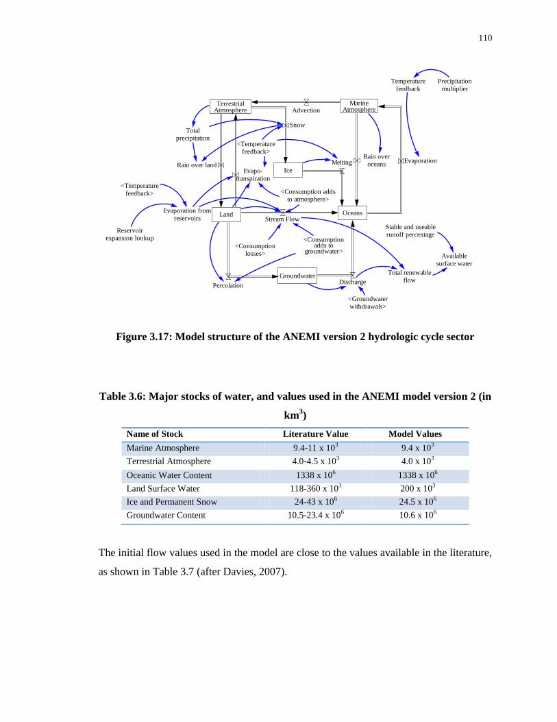
110

Figure 3.17: Model structure of the ANEMI version 2 hydrologic cycle sector

Table 3.6: Major stocks of water, and values used in the ANEMI model version 2 (in

km3)

Name of Stock Literature Value Model Values

Marine Atmosphere 9.4-11 x 103 9.4 x 10

3

Terrestrial Atmosphere 4.0-4.5 x 103 4.0 x 10

3

Oceanic Water Content 1338 x 106 1338 x 10

6

Land Surface Water 118-360 x 103 200 x 10

3

Ice and Permanent Snow 24-43 x 106 24.5 x 10

6

Groundwater Content 10.5-23.4 x 106 10.6 x 10

6

The initial flow values used in the model are close to the values available in the literature,

as shown in Table 3.7 (after Davies, 2007).

TerrestrialAtmosphere

MarineAtmosphere

Ice

OceansLand

Groundwater

Advection

Evapo-transpiration

Rain over land

Snow

MeltingRain over

oceansEvaporation

Stream Flow

PercolationDischarge

Totalprecipitation

Precipitationmultiplier

Temperaturefeedback

<Temperaturefeedback>

Evaporation fromreservoirs

<Temperaturefeedback>

Reservoirexpansion lookup

Stable and useablerunoff percentage

Availablesurface water

Total renewableflow

<Groundwaterwithdrawals>

<Consumption addsto atmosphere>

<Consumptionadds to

groundwater><Consumption

losses>

111

Table 3.7: Hydrologic flows and initial flow values used in the ANEMI model

version 2 (in km3 yr

-1)

Name of Flow Literature Value Model Values

Rainfall over Land 107000-180151 115019

Terrestrial Evapotranspiration 71000-126631 73320

Snowfall over Ice Sheets 2474 2625

Advection (Marine to Terrestrial) 36000-53520 45375

Precipitation over Oceans 398000-481680 489825

Evaporation from Oceans 434000-535200 535200

Melting of Ice Sheets (to Oceans) 2474 2625

Percolation to Groundwater Not available 2312

Groundwater Discharge Not available 2002

Streamflow 36000 39090

Total Renewable Flow 42750 41091

Causal Structure of the ANEMI Version 2 Hydrologic Cycle Sector

The ocean is a vast reservoir of water that works as a collector. It receives water by

rainfall, snow melt, surface flow and ground water discharge from the marine

atmosphere, land ice, land surface and ground water reserve (Figure 3.18). Ocean also

releases water to the marine atmosphere through the evaporation process. This water

travels to the terrestrial atmosphere through the advection process. While traveling over

the land the water vapour condense and produce either snow or rainfall. Over the years

the snow hardens and converts into ice. On the other hand, after touching the land surface

raindrops flow over the land into the river as a surface flow. Some part of the rainwater is

absorbed by the soil through a percolation process and recharges the groundwater

reserve. However, a portion of the rainfall is stored in low-lying areas and reservoirs.

Plants also use water for food production and release the excess water through

transpiration. Through evaporation some water returns to the atmosphere mainly from

open water bodies.

112

Figure 3.18: Causal loop diagram of the ANEMI hydrologic cycle sector

Mathematical Description of the Hydrologic Cycle Sector of ANEMI Model Version 2

The hydrologic cycle sector of the ANEMI model version 2 is adopted from the ANEMI

version 1(Davise, 2007; Davies and Simonovic, 2008), with the addition of sea level rise

and other minor modifications. Therefore, only the main stocks of the natural hydraulic

cycle has been set forth, this section lists the major stock and flow equations of the

hydrologic cycle sector, such as: atmospheric water contents over the ocean and land

(Equations 3.56 and 3.57), water storage in the terrestrial environment, oceans and

ground water (Equations 3.58 to 3.60), and ice storage (Equation 3.61). All flow

equations along with their description are available in Davies (2007).

The equations for the atmospheric water content over the ocean (AM) and land (AL) are

expressed as,

Climate Sector

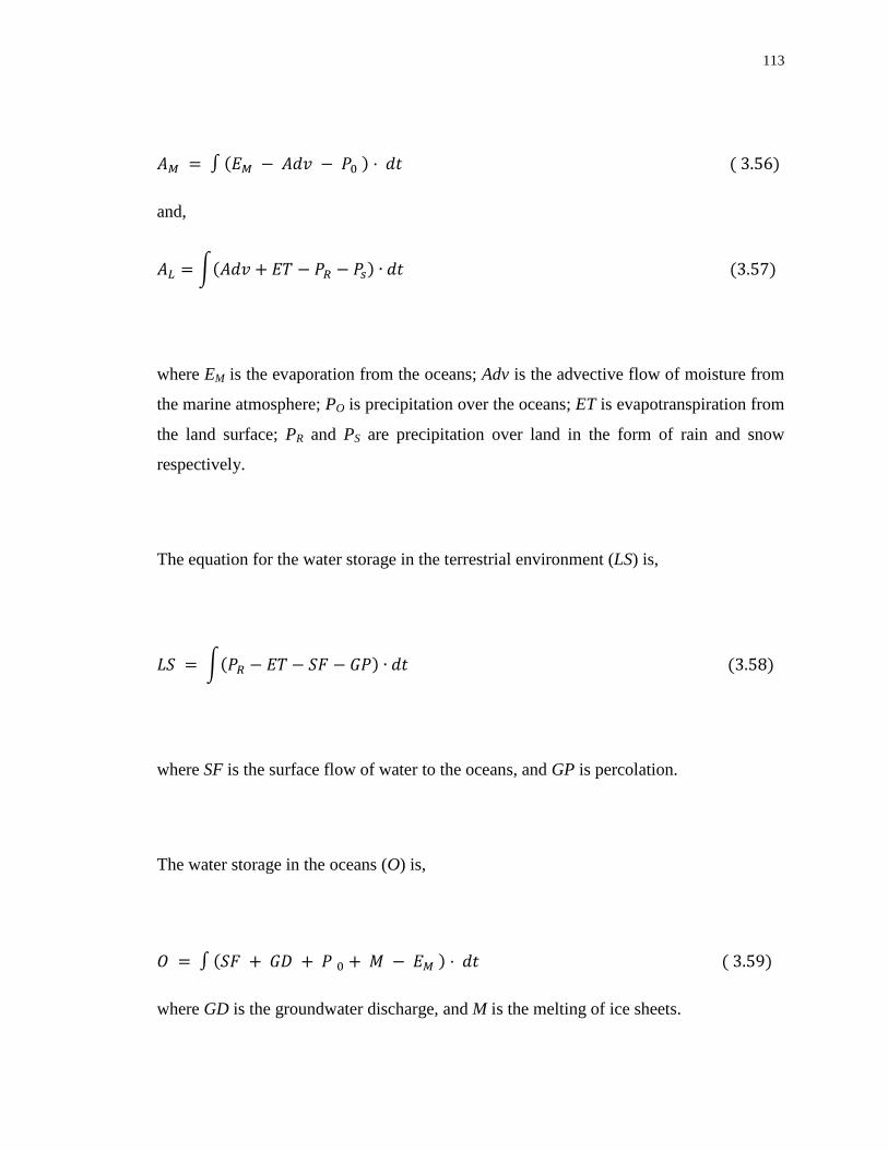
113

and,

where EM is the evaporation from the oceans; Adv is the advective flow of moisture from

the marine atmosphere; PO is precipitation over the oceans; ET is evapotranspiration from

the land surface; PR and PS are precipitation over land in the form of rain and snow

respectively.

The equation for the water storage in the terrestrial environment (LS) is,

where SF is the surface flow of water to the oceans, and GP is percolation.

The water storage in the oceans (O) is,

where GD is the groundwater discharge, and M is the melting of ice sheets.

114

Groundwater storage (GS) and ice storage (IS) are expresses as,

and

(3.61)

3.1.7.2 Water Demand Sector

Primarily surface water availability dominates the anthropogenic water withdrawals and

consumption. As per Davies and Simonovic (2008), the first requirement in computing

anthropogenic water use is to determine a stable or steady-state runoff that occurs at some

fraction of the total average runoff. According to available literature Shiklomanov

(2000), Simonovic (2002b), Alcamo et al. (2003a) came out with different values but

they are within a very close range. Shiklomanov (2000: 18) considers the steady-state

value as 37% of the total volume; the other two researchers choose less than

Shiklomanov (2000:18) but almost same value as one another (Simonovic (2002b) 33%

and Alcamo et al. (2003a) 32%). In this model (ANEMI version 2), available surface

water is chosen as 37%, which is same as Shiklomanov (2000).

In the ANEMI model version 2, human water use is classified as water withdrawals and

water consumption according to Gleick (2000b: 41). In the ANEMI model version 1,

Davies and Simonovic (2008) stressed that returnable water, i.e. the water returned to the

surface flows after it has been used, may cause surface water to become polluted.

Therefore, such an effect is carefully considered in the ANEMI model version 2.

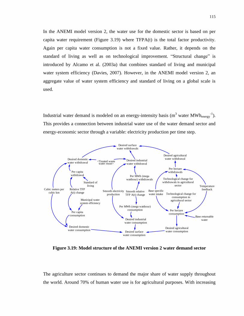
115

In the ANEMI model version 2, the water use for the domestic sector is based on per

capita water requirement (Figure 3.19) where TFPA(t) is the total factor productivity.

Again per capita water consumption is not a fixed value. Rather, it depends on the

standard of living as well as on technological improvement. ―Structural change‖ is

introduced by Alcamo et al. (2003a) that combines standard of living and municipal

water system efficiency (Davies, 2007). However, in the ANEMI model version 2, an

aggregate value of water system efficiency and standard of living on a global scale is

used.

Industrial water demand is modeled on an energy-intensity basis (m3 water MWhenergy

-1).

This provides a connection between industrial water use of the water demand sector and

energy-economic sector through a variable: electricity production per time step.

Figure 3.19: Model structure of the ANEMI version 2 water demand sector

The agriculture sector continues to demand the major share of water supply throughout

the world. Around 70% of human water use is for agricultural purposes. With increasing

Desired surfacewater withdrawals

Desired domesticwater withdrawal

Desired industrialwater withdrawal

Desired agriculturalwater withdrawal

Desired surfacewater consumption

Desired domesticwater consumption

Desired industrialwater consumption

Desired agriculturalwater consumption

Per capitawithdrawal

Per capitaconsumption

Municipal watersystem efficiency

Standard ofliving

Cubic meters percubic km

Per MWh (mega watthour)consumption

Per MWh (megawatthour) withdrawals

Base specificwater intake

Base returnablewater

Per hectareconsumption

Per hectarewithdrawals

Temperaturefeedback

<Treated wastewater reuse>

Relative TFPA(t) change

Technological change forwithdrawals in agricultural

sector

Technological change forconsumption in

agricultural sector

Smooth electricityproduction

Smooth relativeTFP A(t) change

116

population size and climate change, the fresh water used for the agriculture sector is

becoming increasingly scarce. While water-stress appears as a somewhat localized

problem, agricultural water consumption is far reaching and global in its impact.

In this model, the main drivers of agricultural water use are 1) total irrigated area, 2)

change in temperature and 3) technological change. The total irrigated area in both

developed and developing nations expanded rapidly between the 1950s and 1970s. After

the 1970s, the expansion slowed down, because of such factors as the very high cost of

irrigation system construction, soil salinization, depletion of water resources, and

environmental protection problems (Davies and Simonovic, 2008). According to Postel

(1999: 60), ―irrigation has simply begun to reach diminishing returns. In most areas, the

best and easiest sites are already developed.‖

Anthropogenic climate change affects not only available water resources but also water

demand. Using a new global irrigation model with a spatial resolution of 0.50 by 0.5

0,

Döll (2002) carried out the first global analysis of the impact of climate change and

climate variability on irrigation water requirements. This work shows that the computed

long-term average irrigation requirements might change between the 2020s and the

2070s, and that these changes relate back to the variations in irrigation requirements

caused by long-term and interannual climate variability in the 20th century. Döll‘s study

shows clearly that there is every possibility of increased irrigation water requirements

with the projected climate change scenarios.

The last agricultural driver is technological change. According to Davies and Simonovic

(2008), technological change affects the specific water intake value or base irrigation

water requirement per hectare of irrigated land (Shiklomanov, 2000) and their

recommendation present overall efficiency of irrigation worldwide as close to 40%.

117

Causal Structure of the ANEMI Version 2 Water Demand Sector

We have established that surface water use can be classified in terms of consumption and

withdrawal. After Alcamo et al. (2003a), Simonovic (2002b) and Vörösmarty et al.

(2000), we have also assumed that both water withdrawal and water consumption take

place across three sectors – domestic, industrial, and agricultural. In the domestic sector,

water withdrawals and consumption depend on such factors as technological efficiency,

GDP and population (Figure 3.20). In the industrial sector, the ‗intensity‘ of water use is

bound up with the structural and technological changes in energy production.

Figure 3.20: Causal loop diagram of the ANEMI model version 2 water demand

sector

Energy-Economy Sector

Land-Use Sector Climate Sector

Population Sector

118

Mathematical Description of the Water Demand Sector of ANEMI Model Version 2

Desired surface water withdrawal ( ) is the total withdrawal by all three types of water

usage. In this case, desired domestic, industrial and agricultural water withdrawal are

denoted by , , and respectively.

The desired surface water consumption is calculated in the same fashion as Equation

(3.100).

where is desired domestic water consumption, is industrial water consumption,

and is agricultural water consumption.

Domestic water withdrawals and consumption are both dependent on the population size

( ) and its water requirement. However, the amount of desired industrial water

withdrawal is reduced by the reuse of treated water ( ) and desalinated water

( ).

119

where and represents the per capita water withdrawal and consumption

respectively.

Desired industrial water withdrawal and consumption are basically dependent on the

industrial structural water intensity (ISWI), technological change and a function of

electricity production . However, for the calculation of ‗industrial water withdrawal‘,

treated industrial water for reuse ) needs to be subtracted.

Desired agricultural water withdrawal and consumption are calculated based on the

irrigated land ( ), per hectare water withdrawal ( ) and consumption ( ). In

the case of agricultural activities, a significant portion of water comes from treated

wastewater ( ), as well as from ground water withdrawal ( ).

120

where desired agricultural water withdrawal and consumption are denoted by , and

respectively.

3.1.7.3 Water Quality Sector

In the ANEMI model version 2, we have mainly considered surface water in the

modelling of water quality and water availability. Domestic, industrial and agriculture

uses are counted as the main sources of wastewater and water pollution (Figure 3.21).

Shiklomanov (2000) stated that every cubic meter of contaminated wastewater

discharged into the water bodies and streams renders eight to ten cubic meters of clean

water unsuitable for use. Falkenmark (2005), Miller (2006), and Gleick (2000a) also

recognized the importance of including polluted water in the determination of surface

water availability. According to Simonovic (2002b: 263), water pollution is the most

important future water issue on the global scale.‖ It is important to keep the different

characteristics of each water use type in mind when considering the effects of wastewater

on surface water availability (Davies and Simonovic, 2008). A more detailed description

is available in Davies and Simonovic (2008), as a significant portion of the water quality

sector in ANEMI version 2 is adopted from ANEMI version 1.

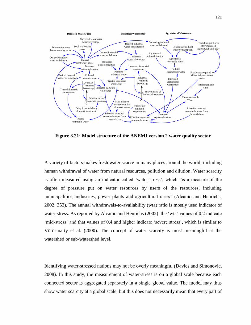
121

Figure 3.21: Model structure of the ANEMI version 2 water quality sector

A variety of factors makes fresh water scarce in many places around the world: including

human withdrawal of water from natural resources, pollution and dilution. Water scarcity

is often measured using an indicator called ‗water-stress‘, which ―is a measure of the

degree of pressure put on water resources by users of the resources, including

municipalities, industries, power plants and agricultural users‖ (Alcamo and Henrichs,

2002: 353). The annual withdrawals-to-availability (wta) ratio is mostly used indicator of

water-stress. As reported by Alcamo and Henrichs (2002) the ‗wta‘ values of 0.2 indicate

‗mid-stress‘ and that values of 0.4 and higher indicate ‗severe stress‘, which is similar to

Vörösmarty et al. (2000). The concept of water scarcity is most meaningful at the

watershed or sub-watershed level.

Identifying water-stressed nations may not be overly meaningful (Davies and Simonovic,

2008). In this study, the measurement of water-stress is on a global scale because each

connected sector is aggregated separately in a single global value. The model may thus

show water scarcity at a global scale, but this does not necessarily mean that every part of

Wastewaterdillution

requirement

Treatedreturnable water

Untreatedreturnable waterEffective untreated

returnable water

Desired domesticwater withdrawal

Desired industrialwater withdrawal

Desired agriculturalwater withdrawal

Industrialpolluted fraction

Agriculturalpolluted fraction

Polluteddomestic water

Pollutedindustrial water

Pollutedagricultural water

Desired domesticwater consumption

Desired industrialwater consumption Desired agricultural

water consumption

Domesticreturnable water

Industrialreturnable water Agricultural

returnable water

Untreatedagriculturalwastewater

Treated domesticwastewater

Untreated domesticwastewater

Treated industrialwastewater

Untreated industrialwastewater

Total returnablewater

Clean returnableWater

Treatedwastewater reuse

Wastewater reusebreakdown by sector

Total wastewaterreuse

Domestic Wastewater Industrial Wastewater Agricultural Wastewater

DomesticTreatmentPercentage

Increase rate ofdomestic treatment

Delay in establishingdomestic treatment

IndustrialTreatmentPercentage

Increase rate ofindustrial treatment

Corrected wastewaterreuse percentage

Max. dilutionrequirement fordomestic water

Freshwater required todilute irrigated waste

water

Effective untreatedreturnable water from

Industrial useEffective untreatedreturnable water from

domestic use

<Total irrigated areaafter increased

agricultural land use>

122

the globe is under water-stress. This inability to distinguish between regional variations

in water-stress is one of the limitations of the global version of the ANEMI model. One

of its unique advantages, however, is the way it takes into account the fresh water

requirement to dilute polluted water in each individual sector.

As previous studies have determined (Gleick, 2000a; Gleick, 2000b; Simonovic, 2002b),

water reuse reduces the water-stress in many of regions of the world, including the

United States, Southern Africa, Israel, and the Middle East (Davies and Simonovic,

2008). The ANEMI model version 2 has adopted a water reuse mechanism or water-

stress indicator into its modelling structure in the same way as ANEMI version 1 does..

In the ANEMI model version 2, the amount of treated wastewater reuse increases over

time, with the rate of increase dependent on (a) the level of global water-stress, (b) the

parameter that represents a real-world infrastructure, and (c) the decision-based delay.

Allocation of the treated wastewater use is originally collected form Gleick (200b), and

presented in Table 3.8.

Table 3.8: Treated wastewater reuse allocations to water use sectors (after Davies,

2007)

Parameter Name Sector Source

Domestic Industrial Agricultural

Treated Wastewater Reuse 10% 30% 60% Gleick (2000b)

Causal Structure of the ANEMI Version 2 Water Quality Sector

Water-stress measures the level of pressure on water resources. In other words, it

expresses how much water is left for ecosystem health. It accounts for the water

withdrawal as well as the return of unused water to the water resources (Figure 3.22). It

123

also considers the amount of fresh water required to dilute the wastewater, so that the

discharged water quality can be within the acceptable range.

Figure 3.22: Causal loop diagram of the ANEMI model version 2 water quality

sector

Mathematical Description of the Water Quality Sector of ANEMI Model Version 2

The water-stress calculation in ANEMI model version 2 considers pollution and follows

the procedures adopted by ANEMI version 1, which are stated in Equations 3.70 and

3.71.

Water Demand Sector

Hydrologic Cycle Sector

124

where is the actual surface water withdrawal and (SF+GD) is the total surface runoff

available for human use. The other option to calculate the water-stress is by reducing

fraction of the total runoff, called ; this can be expressed as,

Where is the effective surface water withdrawal.

Incorporation of the Green Water Consumption

Green water consumption in the global agriculture sector is incorporated to reflect the

water quality effects on water-stress for rainfed cropland runoff. The ANEMI model

version 2 computes the volume of runoff from rainfed cropland and pasture as an area-

weighted fraction of the total runoff from the land surface. Later, the fresh water

requirement to dilute agrochemicals (which are used on the rainfed cropland) is computed

by multiplying the ―rainfed cropland runoff‖ with the ―green water‖ dilution multiplier.

In some regions, food production almost entirely depends on the green water (>95% in

sub-Saharan Africa). Green water is also important for irrigated land, as blue water is

supplied there only to the amount that precipitation water is not sufficient for ensuring

optimal crop growth. Hence, the global agricultural water consumption is much higher

than suggested by figures that refer to blue water only. The outstanding importance of

green water is demonstrated by Rost et al. (2008). Their work strengthens the need for

including green water flows in the assessments of global water resources and water

scarcity.

125

Green water can be broadly classified into green crop water and green pasture water.

Green crop water is basically the overland flow/runoff that comes from agricultural areas

which are not under irrigation (rain feed agricultural area). Green pasture water is the

flow from pasture land.

In a simple way, the rainfed crop land ( ) can be computed by deducting the irrigated

area ( ) from the total agricultural land ( ) as,

while for computing the rainfed cropland runoff, area-weighted method is chosen

considering the equal distribution of runoff over the total biome area. Therefore, the

rainfed cropland runoff ( ) is

where is the total renewable flow, and is the total biome area.

The green crop water dilution requirement is the amount of fresh water required to dilute

polluted crop water. On the basis of the studies done by Chapagain et al. (2006) and

Dabrowski et al. (2009), the dilution requirement of the green crop water is assumed to

be 1:1. So, the green crop water dilution requirement ( ) can be formulated as

follows,

126

Since, as mentioned earlier, the green crop water dilution requirement factor ( is

considered as 1, the above equation can be rewritten as

However, the computation of green water from pasture land is not as straightforward as it

is from rainfed cropland. This is due to the complexity in determining total pasture land.

In the ANEMI model version 2 pasture land is calculated based on the requirements for

increased animal production as a portion of the food supply for the growing population.

Pasture land productivity is therefore a function of the increase in human food production

( ) and Pasture area ( ) calculation for animal product takes the following form

where is the average yield from pasture land.

Runoff over pasture land is computed in a similar fashion as it is for crop land. So the

simplified form of the pasture land runoff ( ) calculation formula is

127

where is the total renewable flow, and is the total biome area.

The green pasture water is relatively less polluted than the runoff from the crop land. In

this study it is assumed to be 1/10 of the crop land. The green pasture water dilution

requirement ( ) can be then written as

As the green crop water dilution requirement is assumed only 10% of the (

polluted water, so the dilution requirement ( will be 0.1 and the simplified form of

the above equation will be

3.1.8 Sea-Level Rise

In order to deal with global water resources, the ANEMI model version 2 incorporates

another important water-related sector: sea-level rise. This sector is introduced into the

ANEMI model version 2 in order to understand more clearly the feedback relationships

between climate, water, and land-use sectors.

128

There are processes in several nonlinearly coupled components of the Earth system that

contribute to sea-level change. It is of great importance to understand them. The climate

change on decadal and longer time scales alters the volume of water in the global ocean

by: (i) thermal expansion, and (ii) the exchange of water between oceans and other

reservoirs (glaciers and ice caps, ice sheets and other land water reservoirs) (IPCC,

2007c). Vertical land movements such as glacial isostatic adjustment, tectonics,

subsidence and sedimentation may influence local sea-levels, but they do not alter ocean

water volume.

The global sea-level rose by about 120m during the several millennia of the last ice age

(approximately 21,000 years ago), and stabilized between 3000 and 2000 years ago

(IPCC, 2007c). Indicators such as marine deposits and lower boundary of mangrove

growth show that the global sea-level did not subsequently change in any significant way

until the late 19th

century. Estimates for the 20th

century showed that the global average

sea-level rose at a rate of about 1.7 mm/yr. It is believed that over the period from 1961

to 2003, thermal expansion contributed on average to about half of the observed sea-level

rise, while melting of the land ice accounted for less than half. Granted, there is some

uncertainty in these estimates.

Understanding global sea-level change is a rather difficult scientific problem. It includes

complex mechanisms and a large number of feedback relationships. Significant

uncertainties persist, even in the projection of thermal expansion. In such a situation, a

semi-empirical model provides a pragmatic alternative to estimate the sea-level response.

In the ANEMI model version 2, the global average near surface air temperature is

considered as the driver for sea-level change. Following Rahmstorf (2007), the sea-level

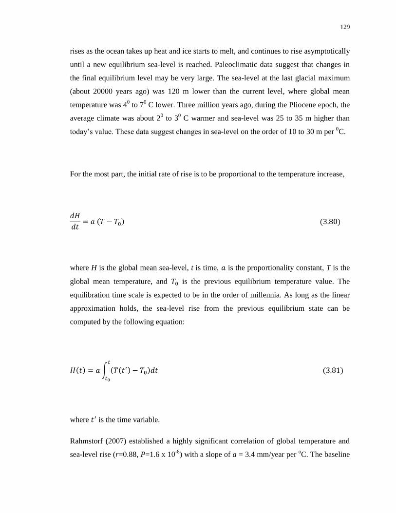
129

rises as the ocean takes up heat and ice starts to melt, and continues to rise asymptotically

until a new equilibrium sea-level is reached. Paleoclimatic data suggest that changes in

the final equilibrium level may be very large. The sea-level at the last glacial maximum

(about 20000 years ago) was 120 m lower than the current level, where global mean

temperature was 40 to 7

0 C lower. Three million years ago, during the Pliocene epoch, the

average climate was about 20 to 3

0 C warmer and sea-level was 25 to 35 m higher than

today‘s value. These data suggest changes in sea-level on the order of 10 to 30 m per 0C.

For the most part, the initial rate of rise is to be proportional to the temperature increase,

where H is the global mean sea-level, t is time, is the proportionality constant, T is the

global mean temperature, and is the previous equilibrium temperature value. The

equilibration time scale is expected to be in the order of millennia. As long as the linear

approximation holds, the sea-level rise from the previous equilibrium state can be

computed by the following equation:

where is the time variable.

Rahmstorf (2007) established a highly significant correlation of global temperature and

sea-level rise (r=0.88, P=1.6 x 10-8

) with a slope of a = 3.4 mm/year per oC. The baseline

130

temperature T0, at which sea-level rise is zero, is 0.5 0C below the mean temperature of

the period 1951-1980.

To date, only a few research groups have worked on the impact analysis of sea-level rise

at a global scale utilizing satellite and remote sensing data in GIS environment. On one

hand, Nicholls et al. (1999), Nicholls (2002 and 2004), and Nicholls and Tol (2006) have

examined the potential impacts of global sea-level rise on coastal flooding. Their

analyses are at the scale of coastal countries and are limited by the assumptions that the

coastal country polygons have a constant slope and that the population distribution within

the polygons is uniform. Dasgupta et al. (2009) on the other hand, considered only 84

developing countries in their impact analyses, leaving developed countries out of their

calculations. A short while later, Xingong et al. (2009) published their research paper

about sea-level rise on a global scale. Using the best available global datasets, they used

GIS methods to assess and visualize the global impacts of potential inundation.

Inundated Area by the Sea-Level Rise

Sea-level rise (SLR) due to climate change is a serious threat to low lying countries with

densely populated coastal regions and significant levels of economic activity. Geographic

Information System (GIS) software is used to overlay the best available, spatially

disaggregated global population and land-use, with the inundation zones corresponding to

projected for 1- 6 m sea-level rise. The inundation data sets are collected from the Center

for Remote Sensing of Ice Sheets (CReSIS), a Science and Technology Center

established by the National Science Foundation (NSF) in 2005

(https://www.cresis.ku.edu/, last accessed August 2011 ).

In order to calculate an inundation area, CReSIS used the Global Land One-km Base

Elevation (GLOBE) digital elevation model (DEM), a raster elevation dataset covering

131

the entire world. Cells in GLOBE have a spatial resolution of 30 arc seconds of latitude

and longitude (approximately one kilometer at the equator), with each land cell in the

grid assigned an elevation value (meters) in whole number increments. The computation

of potentially inundated areas is based on elevation and proximity to the current ocean

shoreline. To determine an inundation area for a sea-level increase of one meter above

the current sea-level, all cells in the DEM that are adjacent to the ocean and that have a

value less than or equal to one are selected and converted to water. In other words, these

cells are inundated in the resulting output.

Impact on Agricultural Land

Agricultural area coverage data is collected from the International Centre for Tropical

Agriculture (CIAT), as well as the overlaid CReSIS based inundation map. The data are

in ARC GRID format, in decimal degrees and datum WGS84 (World Geodetic System).

They are derived from the NASA SRTM data (http://www2.jpl.nasa.gov/srtm/, last

accessed August 2011). The International Centre for Tropical Agriculture (CIAT) has

processed this data to provide seamless continuous topographical surfaces. Areas with

regions with no data in the original SRTM data have been filled in using interpolation

methods.

There is a widespread perception that there is very little new land to bring under

agricultural production. This perception may hold true for specific land-scarce locations

such as Japan, South Asia and the Near East/North Africa. However, it may be wrong for

other parts of the world. There are large tracts of land with varying degrees of agricultural

potential in several countries, most of them in Sub-Saharan Africa and Latin America,

and some in East Asia. In reality, expansion of agricultural land takes place all the time in

countries with growing needs for food production. At the same time, it is also evident that

most of the low laying coastal areas with fertile land are already used for agricultural

132

activities. Thus, the overall rate of increase in agricultural area is very small, even though

global expansion may not be insignificant.

This small rate of increase in agricultural area restricted the reliance of the ANEMI

model version 2 on the forecasted global average agricultural land expansion rate. The

modelling process involved selecting 1990 as the base year for estimating total

agricultural land use. After 1990, the expansion of agricultural land in the low lying

coastal belt is considered negligible.

Impact on Population

Using an innovative approach with the Geographic Information System and remote

sensing data, the Oak Ridge National Laboratory (ORNL) produced the LandScan

population distribution database of the global population distribution

(http://www.ornl.gov/sci/landscan/, last accessed August 2011). The model uses annual

mid-year sub-national population estimates from the US Bureau of Census‘s Geographic

Studies Branch to allocate population counts within administrative units. The LandScan

model uses spatial data and imagery analysis technologies and a multi-variable

dasymetric modelling approach to disaggregate census counts within an administrative

boundary. Since no single population distribution model can account neither for the

differences in spatial data availability, quality, scale, and accuracy, nor the differences in

cultural settlement practices, LandScan population distribution models are tailored to

match the data conditions and geographic nature of each individual country and region.

The binary raster format dataset is used for this analysis. It consists of 20,880 rows and

43,200 columns covering North 84 degrees to South 90 degrees and West 180 degrees to

East 180 degrees. The values of the cells are integer population counts representing an

average population distribution. The dataset has a spatial resolution of 30 arc-seconds

133

and is output in a geographical coordinate system - World Geodetic System (WGS) 84

datum. The 30 arc-second cell, or 0.008333333 decimal degrees, represents

approximately 1 km2 near the equator. Since the data is in a spherical coordinate system,

cell width decreases in a relationship that varies with the cosine of the latitude of the cell.

Thus a cell at 60 degrees latitude would have a width that is half that of a cell at the

equator (cos60 = 0.5). The height of the cells does not vary. Since the cells vary in size,

their values are integer population counts, not population density.

3.2 Feedbacks Between and Within Sectors

In recent years, both water and energy resources management have received an

increasing amount of attention due to their role in socio-economic development, energy

security and the fight against global warming. It became clear, though, that water and

energy resources cannot be evaluated independently of other economic and social

processes. Hence the ANEMI model version 2 considers it important to understand

intersectoral feedback effects.

Integrated Assessment Models (IAMs) have recently been employed in order to study the

effects of climate change policy options. These models help unveil direct and indirect

feedback effects of certain policy choices across various model sectors. The ANEMI

model version 2 is thus well suited for the study of the complex society-biosphere-

climate-energy-economy system. It contains many closed-loop feedback relationships

among its nine model sectors. All of the major elements of the system are endogenous or

included explicitly, so that the dynamic behaviour of the model arises from the system

structure rather than input data.

134

In Figure 3.23, each arrow indicates the connection between the two model sectors. The

title associated with the arrow identifies the element or elements by which those sectors

are connected. The positive and negative polarity associated with each arrow specifies the

direction of change in the sectors connected by the arrow. Here, a positive sign represents

a change of connected variables in the same direction (increase/decrease in one variable

causes an increase/decrease in the other). In the case of a negative sign, the change occurs

in the opposite directions (increase in one variable causes a decrease in the other).

Briefly, the connections between different sectors of the ANEMI model version 2 are:

The carbon and climate sectors through atmospheric CO2 concentrations;

The carbon and food production sectors through emissions index;

The carbon and population sectors through population index;

The climate and hydrologic cycle sectors through surface temperature change;

The climate and energy-economy sectors through surface temperature change;

The climate and population sectors through surface temperature change;

The hydrologic cycle and water demand sectors through surface water

availability;

The hydrologic cycle and population sectors through water-stress;

The water demand and hydrologic cycle sectors through water consumption;

The water demand and water quality sectors through wastewater treatment;

The hydrologic cycle and food production sectors through water-stress;

The water quality and water demand sectors through wastewater reuse;

The population and water demand sectors through total water demand;

The population and land-use sectors through forest and grassland clearing and

burning;

The population and energy-economy sectors through consumption per capita and

labour;

The energy-economy and water demand sectors through economic output (GDP),

water use efficiency and electricity production;

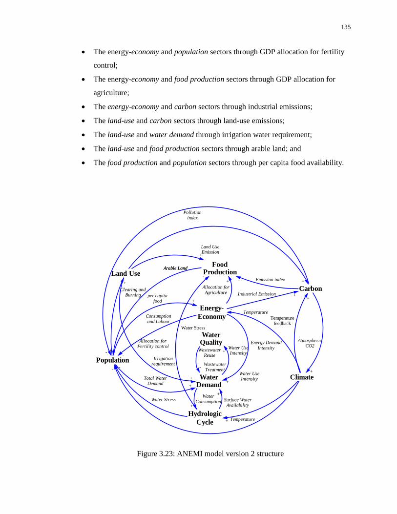
135

The energy-economy and population sectors through GDP allocation for fertility

control;

The energy-economy and food production sectors through GDP allocation for

agriculture;

The energy-economy and carbon sectors through industrial emissions;

The land-use and carbon sectors through land-use emissions;

The land-use and water demand through irrigation water requirement;

The land-use and food production sectors through arable land; and

The food production and population sectors through per capita food availability.

Figure 3.23: ANEMI model version 2 structure

Land Use

Energy-

Economy

Carbon

Climate

Hydrologic

Cycle

Population

+

WaterDemand

+

+

+

+

-

+

++

Land UseEmission

Clearing andBurning

Consumptionand Labour

Water Stress

Temperature

AtmosphericCO2

Industrial Emission

Total WaterDemand

WaterConsumption Surface Water

Availability

Water UseIntensity

Temperature

Water UseIntensity

Energy DemandIntensity

WaterQuality

WastewaterTreatment

WastewaterReuse

-

+

+

-

FoodProduction

+

Arable Land

+

Allocation forAgriculture

Water Stress

- Emission index

-

per capitafood

+-

Pollutionindex

Allocation forFertility control

-

++

Temperaturefeedback

-

+

Arable Land

Irrigationrequirement

136

The following two sub-sections are divided according to the feedback descriptions of

water and non-water sectors, since the water demand, water quality, and hydrologic cycle

(water quantity) sectors are interdependent and essentially inseparable.

3.2.1 Feedbacks within the ANEMI Model Version 2 Water Sectors

The hydrologic cycle, water demand, and water quality sectors are very tightly linked

with each other through total available water, water consumption and withdrawal,

polluted waste water and water-stress, and waste water treatment and reuse. Thus they

form a closed loop system with following feedback relations:

High intensity of water use requires high amount of water withdrawal from the

available water sources;

Increased evaporation reduces the amount of available water from soil and open

water bodies;

Decrease of snowmelt can lead to less stream flow and therefore a lower amount

of available water;

Decrease in the amount of available water and high water withdrawals lead to

higher water-stress;

High water-stress leads to alternative choices such as larger groundwater

withdrawals, introduction of desalination, and wastewater treatment and reuse.

As shown in Figure 3.24, the tight structure of the water sectors requires the introduction

of more feedback relationships than one finds in the other sectors of the model. The

major links of each sector are discussed further.

137

Figure 3.24: Feedback loops within ANEMI model version 2 water sectors

Water-stress is a measure of water scarcity, and is calculated as the ratio between the

effective withdrawal (including effective blue water withdrawal and withdrawals for

dilution requirement) and the total renewable flow.

where represents the total water withdrawal for domestic, industrial and agricultural

use along with the water required for dilution purpose. is the total renewable flow for

human use, measured in km3 yr

-1, which is the sum of the global annual surface flow and

groundwater discharge.

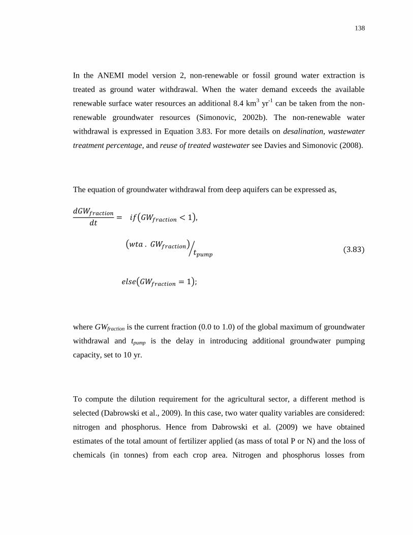
138

In the ANEMI model version 2, non-renewable or fossil ground water extraction is

treated as ground water withdrawal. When the water demand exceeds the available

renewable surface water resources an additional 8.4 km3 yr

-1 can be taken from the non-

renewable groundwater resources (Simonovic, 2002b). The non-renewable water

withdrawal is expressed in Equation 3.83. For more details on desalination, wastewater

treatment percentage, and reuse of treated wastewater see Davies and Simonovic (2008).

The equation of groundwater withdrawal from deep aquifers can be expressed as,

where GWfraction is the current fraction (0.0 to 1.0) of the global maximum of groundwater

withdrawal and tpump is the delay in introducing additional groundwater pumping

capacity, set to 10 yr.

To compute the dilution requirement for the agricultural sector, a different method is

selected (Dabrowski et al., 2009). In this case, two water quality variables are considered:

nitrogen and phosphorus. Hence from Dabrowski et al. (2009) we have obtained

estimates of the total amount of fertilizer applied (as mass of total P or N) and the loss of

chemicals (in tonnes) from each crop area. Nitrogen and phosphorus losses from

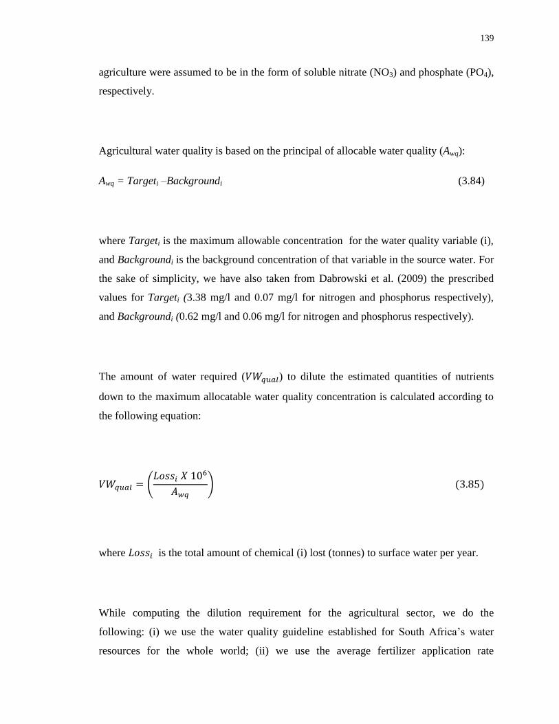
139

agriculture were assumed to be in the form of soluble nitrate (NO3) and phosphate (PO4),

respectively.

Agricultural water quality is based on the principal of allocable water quality (Awq):

Awq = Targeti –Backgroundi (3.84)

where Targeti is the maximum allowable concentration for the water quality variable (i),

and Backgroundi is the background concentration of that variable in the source water. For

the sake of simplicity, we have also taken from Dabrowski et al. (2009) the prescribed

values for Targeti (3.38 mg/l and 0.07 mg/l for nitrogen and phosphorus respectively),

and Backgroundi (0.62 mg/l and 0.06 mg/l for nitrogen and phosphorus respectively).

The amount of water required ( ) to dilute the estimated quantities of nutrients

down to the maximum allocatable water quality concentration is calculated according to

the following equation:

where is the total amount of chemical (i) lost (tonnes) to surface water per year.

While computing the dilution requirement for the agricultural sector, we do the

following: (i) we use the water quality guideline established for South Africa‘s water

resources for the whole world; (ii) we use the average fertilizer application rate

140

(computed for maize, wheat, sugarcane and citrus) for all types of crops; and (iii) we take

into account only the irrigated agricultural areas while calculating the dilution

requirement. These assumptions are introduced due to the unavailability of information

related to total fertilizer use in agriculture.

3.2.2 Feedbacks in the ANEMI Model Version 2 Non-Water Sectors

The carbon sector has two major feedbacks producing radiative forcing that leads to

increase in temperature. In climate sector atmospheric CO2 is translated in the radiative

forcing with the forcing equation. The other sources of radiative forcing are computed

from other gases: methane, nitrous oxide, chlorofluorocarbons and other Montreal

protocol gases. All the forcings are then added together to feed into the climate sector as

an input variable.

where is for total forcing in W m-2

; , ,and stand for radiative forcing

from carbon-dioxide, chlorofluorocarbon and nitrous oxide respectively. represents

Montreal Protocol and other gases; while CA and CA0 denote the current and the initial

atmospheric carbon dioxide concentrations respectively.

141

The climate sector plays a very important role in the ANEMI model version 2. Its product

and temperature change impact almost all the sectors of the model. The population, food

production, hydrologic cycle, land-use, water demand, and water quality sectors are

connected with the climate sector through the global temperature. In many cases the

temperature rise may have more negative than positive effects. Increased temperature

could boost the evaporation from a water body and increase the water-stress by lowering

the stock of available water. However, there is a chance that if the temperature change

takes place, some countries of the northern hemisphere (Canada included) could be able

to expand their agricultural areas further north. Granted, the increase in temperature could

potentially increase the irrigation demand, which may then act as a constraint for

agricultural land expansion.

For estimating the impact of the current trend in climate change on the energy-economic

sector, the climate damage function is introduced. The climate damage function assumes

a relationship between economic damage and the extent of warming. According to

Nordhaus and Boyer (2000), the specific relationship between global temperature

increase and income loss is expressed by damage function in quadratic form:

(3.89)

where is the damage from climate change, as a fraction of output and atmospheric

temperature increase (in degree Celsius) over year 1900 level, and are parameters

of the damage function.

142

The increase in temperature affects the global hydrologic cycle by changing the intensity

of evaporation, precipitation pattern, starting day of snow melt, and so on. The simplest

way of introducing the effect of temperature change in the hydrologic cycle is by defining

a fixed temperature multiplier. In many cases, this linear relationship may not be valid

because of non-linear feedback effects. The current understanding of Arctic ice melt

provides an interesting example of this. Light covered surfaces such as ice and snow

reflect the incoming solar radiation back into outer space, while dark covered surfaces

such as oceans and land absorb the incoming radiation, which increases the temperature

and contributes to further warming. The higher global temperature triggers the melting of

Arctic sea-ice and as the sea-ice melts there is less ice to reflect the incoming solar

radiation and more open ocean to absorb the solar energy. This absorbed energy triggers

a positive feedback that warms the ocean further causing more ice to melt faster.

Huntington (2006) stated that global precipitation is energy limited rather than moisture

limited, and so precipitation is expected to rise by 3.4% per 1 surface temperature

increase. This leads to the following functional relationship, which is extracted from

Davies and Simonovic (2008):

where is the temperature multiplier, which takes its value from , the

precipitation multiplier is measured in Kelvin, which denotes the change in surface

temperature; is a fixed value of 3.4% K-1

.

143

This simple relationship is used to establish feedback links between climate, water use,

water demand, and evaporation calculation. To model the effects of climate change on

irrigation water requirements, the ―per hectare water withdrawals‖ and ―per hectare water

consumption‖ are multiplied by the same ‗temperature multiplier‘. The carbon sector of

the ANEMI model version 2 deals with the total carbon balance at the global scale, even

though a significant portion of carbon is produced in the energy-economy sector.

The population sector is linked to the land-use sector in the same way as Davies (2007),

which followed the approach of Goudriaan and Ketner (1984). For further details readers

are directed to Davies and Simonovic (2008).

The emissions from the energy-economy sector are directly imported and added to the

carbon sector. Carbon emissions from each type of energy source are calculated based on

energy consumption and carbon content. The following equation computes the CO2

emissions in 106 tons C.

where = annual production in 106 tons of fossil fuel equivalent ( approx. 11.2%), FOi

stands for effective fraction oxidized in the year of production and Ci for carbon content

in tons C per ton coal equivalent/ tons C per thousand 1012

joules. The conversion factor

used for 1 ppmv of atmosphere CO2 = 2.13 Gt C.

Each of the three water related sectors is linked with both food production and population

sectors through the ‗water-stress‘ variable. The link between water and social

144

development is reflected in the water impacts on health. Without safe drinking water,

humans cannot survive. Waterborne diseases are amongst the most common causes of

illness and death, and the majority of people affected by them are living in developing

countries. With the steady increase in population, people must find a way to add a huge

amount of water to the global water supply every year. Moreover, some areas are

expected to get a lower amount of rainfall due to climate change, and therefore these

areas will face an alarming level of ‗water-stress‘. Human life expectancy is therefore

expressed as an inverse function of ‗water-stress‘ level.

The agricultural sectors of many regions in the world fully depend on water supply, and

this supply is limited. Irrigation continues to play a crucial role in the agricultural sector,

but the limitation in water availability serves as one of the constraints for increase of the

agricultural land. The agricultural sector is also inversely related to water-stress.

3.2.3 Summary

In this chapter, we have distinguished between two types of feedbacks: the intersectoral

feedbacks within the water sectors and the intersectoral feedbacks within rest of the

sectors. The overall intention of the chapter was thus to help the reader trace the effects

of a change in a variable in one sector and the subsequent reactions and changes that

occur in other sectors.

Figure 3.1 and Figure 3.24 facilitate the understanding of the basic structure of the model.

They can guide the reader through the identification of feedback polarity, as well as the

polarity of feedback loops that connect the different sectors of the model.

145

In order to present a clear view of the structural difference of the ANEMI model version

2 and version 1, Table 3.9 summarizes the improvements and new additions that are

made in the ANEMI model version 2. The first column of the table states all the sectors

of the ANEMI model version 2, while the second describes the type of changes (whether

it is new, old or modified compared to ANEMI version 1), followed by a brief description

of the corresponding changes are mentioned in the third column.

Table 3.9: Summary of the ANEMI model modifications

Sectors Change between version 1 and 2 Description of change Climate added a simplified climate sector

and modified the old one, so that user can have option to choose between old and new according to the complexity of the work

Introduction of the simplified climate sector Addition of the radiative forcing from other GHGs

Carbon Modified Introduction of the temperature effect on CO2 solubility in ocean

Hydrologic Cycle

Modified Incorporation of sea-level rise

Water Demand

Modified Industrial water demand is linked with the electricity production

Water Quality Modified New dilution factor based on the type of water usage and pollutant concentration

Population Replaced New 4 age-group population sector Feedback from carbon sector by pollution index Feedback from climate sector Feedback from food production sector

Land-use No change No change

Food Production

New New sector

Energy-Economy

Replaced Introduction of the optimization simulation scheme to reflect general equilibrium theory of economics The simulation is carried out till 2100, whereas ANEMI version1 can be simulated up 2010

146

CHAPTER 4

4 GLOBAL MODEL EXPERIMENTATION

This chapter deals with model experimentation, and covers a wide range of activities:

from model calibration to result analyses. First, we set forth a performance analysis of the

ANEMI model version 2, comparing the results of its simulation with historical

observations. Then we provide a descriptive introduction to the model‘s scenario

formulation, implementation and simulation. Finally, the chapter concludes model

analysis results.

4.1 ANEMI Model (version 2) Performance

Traditional model calibration is a process that consists of changing the values of model

input parameters to match observed behaviour in accordance with some acceptable

criteria. However, in the context of global change research, the process of model

calibration faces a key limitation: there is only one Earth, and therefore only one set of

globally-aggregated data available. Our model calibration therefore proceeded in several

steps: 1) parameters were first adjusted in individual sectors, 2) the individually-

calibrated sectors were checked against historical data and against data from other

models, and 3) the sectors were integrated and model output was again tested against

other sources. The ANEMI model version 2 is based on previous modelling work. Hence

many of its sectors use the same parameter values as other models. In cases where the

parameters derived from well-established, quantifiable, and measurable characteristics,

we checked the values obtained against real-world data. However, in cases where the

147

parameters had no strong physical basis, we checked the effects of parameter variations

on whole-model behaviour through sensitivity analysis.

In order to validate a model, one must compare the estimated variables to historical data.

The validation process describes the model‘s underlying mechanics, in order to determine

the logic and accuracy of the modeler‘s representation of the real world situation. Model

validation therefore determines how adequately the model‘s underlying fundamental

rules and relationships are able to capture the targeted emergent behaviour, as specified

within the relevant theory and as demonstrated by field data.

The calibration or validation of a model‘s performance requires both qualitative and

quantitative measures. These measures involve graphical comparisons and statistical

tests. Based on data availability, a satisfactory number of yearly comparisons have been

performed on the ANEMI model version 2. Simulated values in Table 4.1 to Table 4.12

provide information on the model‘s performance.

As stated above, the individual sectors are developed and calibrated before combining all

the sectors together. An individual sector must first demonstrate a satisfactory

performance with reasonable parameter values before the next step of integration can take

place. During the isolated runs, the intersectoral feedbacks are not activated. Rather, the

related variables from other sectors are predefined. With the establishment of the

feedback relationships, the model showed a deviation from the performance obtained

through the simulation of individual sectors. Hence further adjustments of model

parameters were required.

It is worthwhile to mention that this model of the society-biosphere-climate-energy-

economy system is not meant to predict the future. Rather, it aims to help one understand

148

the behavior of the system and to understand the behavioural consequences of various

policy options.

The rest of section 4.1 presents the performance of a feedback based fully integrated

society-biosphere-climate-economy-energy system through the analyses of the model‘s

base run. The individual sectors of the fully integrated version of the ANEMI model are

thus tested against measurements and literature data from 1980 to 2010 (Table 4.1 to

Table 4.12). Even with a small number of exogenous inputs (mainly future fossil fuel

discovery), this comprehensive feedback based integrated modelling system proves its

superiority by producing a very close agreement with the real world data.

4.1.1 Water Use

In the last one hundred years, water use has been growing rapidly as a result of increasing

water demand and population growth. For the most part, this enormous (nearly fivefold)

increase in water use is a result of an expanding agricultural sector. In the ANEMI model

version 2, water consumption and withdrawal are calculated for three individual groups

(domestic, industrial and agricultural). The model results are compared to IHP (2000)

data, projections by Simonovic (2002b), Alcamo et al. (2003b), and Cosgrove and

Rijsberman (2000). The calibrated ANEMI model version 2 agrees well with both the

historical data (Table 4.1) and the projections available in the literature (Table 4.2).

149

Table 4.1: Assessed global water withdrawals and consumption (in km3/yr)

Year 1980 1990 1995

IHP(2000)

Domestic Withdrawals 219 305 344

Domestic Consumption 38.3 45.0 49.8

Industrial Withdrawal 713 735 752

Industrial Consumption 70.9 78.8 82.6

Agricultural Withdrawal 2112 2425 2504

Agricultural Consumption 1445 1691 1753

Simulated Value

Domestic Withdrawals 210 315 349

Domestic Consumption 39 48 53

Industrial Withdrawal 560 570 615

Industrial Consumption 57 62 70

Agricultural Withdrawal 2100 2600 2800

Agricultural Consumption 1440 1880 1980

Table 4.2: Projected global water withdrawals and consumption (in km3/yr)

Year 2000 2010 2025

IHP(2000)

Domestic Withdrawals 384 472 607

Domestic Consumption 52.8 60.8 74.1

Industrial Withdrawal 776 908 1170

Industrial Consumption 84 120 167

Agricultural Withdrawal 2605 2817 3189

Agricultural Consumption 1834 1987 2252

Simonovic (2002b)

Domestic Withdrawals - - 723

Industrial Withdrawals - - 520

Agricultural Withdrawals - - 3554

Cosgrove and Rijsberman(2000)

Domestic Withdrawals - - 900

Domestic Consumption - - 100

Industrial Withdrawal - - 900

Industrial Consumption - - 120

Agricultural Withdrawal - - 2300

Agricultural Consumption - - 1700

Simulated Values

Domestic Withdrawals 413 572 752

Domestic Consumption 62 80 93

Industrial Withdrawal 690 880 987

Industrial Consumption 80 90 105

Agricultural Withdrawal 2900 3100 3300

Agricultural Consumption 2070 2210 2350

150

4.1.2 Sea-Level Rise

Inundated Area by Sea-Level Rise

For the global inundated land area calculation, Xingong et al. (2009) used the GLOBE

dataset because of its improved version of the GTOPO30 data. This data was compiled

from the best global and regional raster and vector elevation datasets available at the time

of compilation (Hastings and Dunbar, 1998). Dasgupta et al. (2009) used NASA‘s WVS

(World Vector Shoreline) dataset

(http://gcmd.nasa.gov/records/GCMD_WVS_DMA_NIMA.html, last accessed Aug,

2011). In order to calculate the total inundated area from changes in sea-level rise, the

ANEMI model version 2 uses the lookup table produced from Xingong et al. (2009).

With this table, the ANEMI model version 2 show that the sea-level may rise by one

meter by 2092-93 and that 1,098,000 Km2

area will be inundated at the end of 21st

century when the sea-level rises to 1.15 meter.

Sea-Level Rise Impact on Agricultural Land

In order to calculate the impact of sea-level rise on agricultural land, the ANEMI model

version 2 requires the percentage value of impacted agricultural land extracted from

Dasgupta et al. (2009). Simulated results show that the total impacted agricultural area

would be 46,679 Km2 at the end of 21

st century.

Sea-Level Rise Impact on Population

In the ANEMI model version 2, the computation of the effect of sea-level rise on human

population is done exogenously because of insufficient data and the global nature of the

population structure in the model (i.e. no spatial distribution along the coast lines). To

overcome this constraint, a combined approach is carried out where an average

percentage of impacted population is computed from Dasgupta et al. (2009) and Xingong

151

et al. (2009). This process is carried out for each level of sea-level rise. The computed

value of 134 million impacted people is obtained for 1-meter sea-level rise.

Nicholls (2002) estimated that the number of people exposed to flooding by storm surges

in 2100 would range between 503 and 755 million people at 96 cm sea-level rise. The

ANEMI model version 2 does not consider storm surges; it considers sea-level rise only

as a consequence of ocean thermal expansion and ice melt.

4.1.3 Global Population

The United Nations (UN) Population Division provides population data over the period

of 1950 to 2050, out of which projected data started from 2005. The UN Population

Division is under the United Nations Department of Economic and Social Affairs

(UNESA); it is responsible for the monitoring and appraisal of the broad range of areas in

the field of population. The International Institute for Applied Systems Analysis (IIASA)

also provides a 100 year population projection. This projection was last revised in 2007.

The IIASA is an international research organization that conducts policy-oriented

research into problems that are too large or too complex to be solved by a single country

or academic discipline. Other scenarios that provide projections of future population

growth include Nakicenovic and Swart (hereafter, IPCC 2000), Alcamo et al. (1996) and

RCPs (Moss et al., 2008). Nordhaus (2007) used the DICE model to simulate future

population growth, and the results have been well accepted by the integrated assessment

modelling communities.

As the historical global population comparison (Table 4.3) attests, the global ANEMI

model version 2 is capable of generating a trend in population growth close to the

historical data (UNESA, 2006). The simulated population value from the ANEMI version

1 (Davies and Simonovc, 2008) is also included for comparison.

152

A comparison of the simulated future population values is performed using data from a

variety of other projection scenarios (Table 4.4, and Figure 4.1 ). In a few cases, the total

global population starts to decline after 2075, but in most of the projections only the

population growth rate declines, not the total population. The simulated result from the

ANEMI model version 2 shows the same tendency of lower population growth rate.

Table 4.3: Comparison of historical global population (in billions)

Year 1980 1985 1990 1995 2000 2005

UNESA (2006) 4.45 4.86 5.30 5.72 6.12 6.51

ANEMI version 1 (Davies

and Simonovic, 2008)

4.51 4.91 5.31 5.7 6.09 6.47

ANEMI version 2 simulated

population

4.44 4.75 5.13 5.52 5.91 6.32

Table 4.4: Comparison of future global population (in billions)

Year 2010 2025 2050 2075 2100

UNESA (2006) 6.91 8.01 9.15

IPCC (2000) Scenario A1B - 7.66 8.70 - 7.10

IPCC (2000) Scenario A2 - 8.81 11.3 - 15.10

IPCC (2000) Scenario B1 - 7.82 8.70 - 7.00

RCP8.5 (Riahi et al.,2007) 7.0 8.30 10.2 11.80 12.02

RCP6 (Fujino et al., 2006; and Hijioka et al.,

2008)

7.0 7.95 9.04 9.095 9.09

RCP4.5 (Clarke et al., 2007; Smith et al.,

2006; and Wise et al., 2009)

7.0 7.95 9.01 9.030 9.025

RCP3-PD (van Vuuren et al., 2006; 2007) 7.0 7.95 8.095 9.00 8.060

Alcamo et al. (1996), Base A 7.11 - 10.10 - 11.50

Alcamo et al. (1996), Base B 6.70 - 7.84 - 6.43

Fiddaman (1997) 7.23 8.41 9.98 11.10 11.80

Nordhaus and Boyer (2000) 6.88 7.96 9.29 10.20 10.70

DICE_2007 (Nordhaus, 2007) 6.93 8.02 8.55 8.67 8.69

ANEMI version 1 (Davies and Simonovic,

2008)

6.84 7.87 9.36 10.60 11.70

IIASA (low) 6.74 7.44 7.78 7.15 6.16

IIASA (medium) 6.82 7.79 8.75 8.87 8.39

IIASA (high) 6.88 8.16 9.90 10.80 11.05

ANEMI version 2 simulated population 6.77 7.98 9.32 9.97 10.53

153

Figure 4.1: Comparison of global population projection

4.1.4 Energy based CO2 Emissions and Energy Production

In this study the energy production is computed considering the individual energy

sources: coal, oil, natural gas, hydro, nuclear and alternative. However, the net demand of

energy is divided into two categories; 1) heat energy demand, and 2) electric energy

demand. According to IEA (2007:25), about 78% of the world‘s energy demand comes

from heat-energy, while the remaining 22% is from electric-energy. Non-renewable

energy resources, mainly fossil fuels are used in the heat energy production. The relative

costs of heat energy versus electric energy determine the mix of sources used in future

production, reserve, as well as overall energy use.

The available energy production data for both heat and electric are extracted with unit

adjustment from the Energy Information Administration (EIA) database (available at

http://www.eia.gov/countries/data.cfm#undefined, last accessed December, 2011). Comparison

plots in Figure 4.2 and Figure 4.3 show a satisfactory match between the observed and

simulated data. However, it should be mentioned at this point that while calibrating the model,

2.0

4.0

6.0

8.0

10.0

12.0

14.0

1980 2000 2020 2040 2060 2080 2100

Po

pu

lati

on

(b

illi

on

)

Time

Global Population

ANEMI version 2

IPCC (median)

DICE_2007

ANEMI version 1

154

one of the objectives was to match the observed data perfectly so that the parameter values of the

energy production could be computed properly.

Figure 4.2: Comparison of heat energy production

Figure 4.3: Comparison of electric energy production

0

1

2

3

4

5

6

1980 2000 2020 2040 2060 2080 2100

Ene

rgy

(10

11

GJ)

Time

Energy Used for Heat Energy Production

ANEMI version 2

EIA data

0

1

2

3

4

5

6

1980 2000 2020 2040 2060 2080 2100

Ene

rgy

(10

11

GJ)

Time

Energy Used for Electricity pruction

ANEMI version 2

EIA data

155

The two main sources of CO2 emissions are energy production and land-use change

(which affects radiative forcing). The emissions from the fossil fuel burning represent

the most significant contribution. Therefore, the extent of future climate change is

heavily dependent on the fossil fuel burning rate for both heat and electric energy

production. The ANEMI model version 2 is extremely sensitive to fossil fuel prices and

follows a market clearing mechanism. The concept of a market clearing mechanism is a

simplifying assumption set forth by the new classical or neoliberal school of economics:

it is the assumption that markets tend toward prices that ensure the clearance of all

surpluses, or that the quantity supplied will always eventually equal the quantity

demanded. The IPCC (2000) and Marland et al. (2008) data show a good match with the

ANEMI version 2 simulated results, with some level of overestimation from 1980 to

2000 (Table 4.5 and Figure 4.4).

Table 4.5: Comparison of historical industrial emissions (in Gt C/yr)

Year 1980 1985 1990 1995 2000 2005

IPCC (2000) Scenario A1B - - 6.0 - - -

IPCC (2000) Scenario A2 - - 6.0 - - -

IPCC (2000) Scenario B1 - - 6.0 - - -

Marland et al. (2008) 5.35 5.44 6.16 6.4 6.75 7.99

ANEMI version 1 (Davies and

Simonovic, 2008)

5.11 - 5.96 6.32 6.77 -

ANEMI version 2 simulated

emissions

5.38 5.78 6.21 6.68 7.21 7.86

In case of simulated future emissions, the model behaves in a logical fashion till 2050.

The results are compliant with most of the projections from IPCC (2000), Alcamo et al.

(1996), Nordhaus and Boyer (2000), Goudriaan and Ketner (1984) and RCPs (Moss et

al., 2008). After 2050, the emissions generation from the energy sector starts to decline

and emissions follow a very different path than other projections available in the

literature. For example, the 2007 version of DICE model (Nordhaus, 2007) shows

incrementally increasing rates of emissions till the end of this century (Figure 4.4). But

156

the ANEMI version 2 simulation results show that in comparison to the current state there

will be almost zero increase in emissions by then (Table 4.6). However, there will be a

peak in the industrial emissions around the mid of the 21st century. Such behaviour is not

unexpected, since in-depth investigation reveals that if the present extraction trend

continues the world would be out of available known fossil fuel reserves by 2100. Hence

the industrial emissions increment rate approach zero value. It is assumed that nuclear,

hydro and alternative energy sources will take care of future energy demand, thereby

leaving almost zero fossil fuel energy based emissions in the atmosphere.

Figure 4.4: Comparison of industrial carbon emissions

0.0

2.0

4.0

6.0

8.0

10.0

12.0

14.0

16.0

18.0

20.0

1980 2000 2020 2040 2060 2080 2100

Ind

ust

rial

Em

issi

on

s (G

t C

/yr)

Time

Industrial Carbon Emissions

ANEMI version 2IPCC (B1)IPCC (A1B)DICE_2007ANEMI version 1

157

Table 4.6: Simulated industrial emissions (in Gt C/yr)

Year 2010 2020 2025 2030 2050 2075 2100

IPCC (2000) Scenario A1B - 12.1 - - 16.0 - 13.1

IPCC (2000) Scenario A2 - 11.0 - - 16.5 - 28.9

IPCC (2000) Scenario B1 - 10 - - 11.7 - 5.2

RCP8.5 (Riahi et al.,2007) 8.926 11.538 - 13.839 20.205 26.684 28.740

RCP6 (Fujino et al., 2006; and

Hijioka et al., 2008)

8.512 8.95 - 9.995 13.044 16.894 13.753

RCP4.5 (Clarke et al., 2007;

Smith et al., 2006; and Wise

et al., 2009)

8.607 9.872 - 10.953 11.031 5.65 4.203

RCP3-PD (van Vuuren et al.,

2006; 2007)

8.821 9.288 - 7.157 3.186

Alcamo et al. (1996), Base A 11 13 - 14 15.5 18.0 22.0

Alcamo et al. (1996), Base B 8 10 - 9.5 9.0 8.0 8.0

Goudriaan and Ketner (1984),

Low Emission

- - - 8.9 - - -

Goudriaan and Ketner (1984),

High Emission

- - - 16.2 - - -

DICE _2007 (Nordhaus,

2007)

8.2 9.5 10.0 10.7 13.0 16.0 19.0

ANEMI version 1 (Davies

and Simonovic, 2008)

7.54 8.19 - 8.82 10.11 11.93 13.98

ANEMI version 2 simulated

emissions

8.18 8.82 9.4 9.92 10.49 7.35 8.3

4.1.5 Gross Domestic Product (GDP)

The gross domestic product (GDP) is the most commonly used indicator to express

economic wealth at a global or regional scale. Although it is usually calculated on an

annual basis, GDP can represent the monetary value of all finished goods and services

produced within a country‘s borders in any specific time period. It thus includes at any

given time all private and public consumption, government outlays, investments and

exports less imports that occur within a defined territory. Nordhaus (2007) used the DICE

model to simulate the future GDP and produced a well-accepted result by the global

modelling community. As shown in Figure 4.5, the simulated GDP of the ANEMI model

version 2 is not too apart from the Nordhaus value, thereby proving its acceptable

representation of the global energy-economy sector.

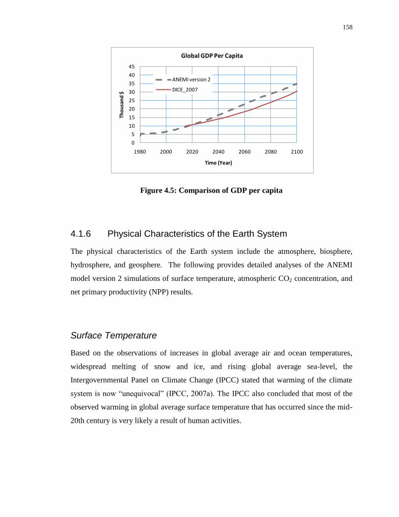
158

Figure 4.5: Comparison of GDP per capita

4.1.6 Physical Characteristics of the Earth System

The physical characteristics of the Earth system include the atmosphere, biosphere,

hydrosphere, and geosphere. The following provides detailed analyses of the ANEMI

model version 2 simulations of surface temperature, atmospheric CO2 concentration, and

net primary productivity (NPP) results.

Surface Temperature

Based on the observations of increases in global average air and ocean temperatures,

widespread melting of snow and ice, and rising global average sea-level, the

Intergovernmental Panel on Climate Change (IPCC) stated that warming of the climate

system is now ―unequivocal‖ (IPCC, 2007a). The IPCC also concluded that most of the

observed warming in global average surface temperature that has occurred since the mid-

20th century is very likely a result of human activities.

0

5

10

15

20

25

30

35

40

45

1980 2000 2020 2040 2060 2080 2100

Tho

usa

nd

$

Time (Year)

Global GDP Per Capita

ANEMI version 2

DICE_2007

159

Vinnikov et al. (2006) analyzed the satellite data and concluded that the global surface

temperatures changed by 0.2°C per decade between 1978 and 2004. This value is also

consistent with the studies by Brohan et al. (2006) and Smith and Reynolds (2005). They

calculated temperature anomalies in degrees Celsius based on the deviation from a long-

term 1961-1990 temperature average. Nordhaus and Boyer (2000) calculated their

temperature anomaly based on the pre-industrial average surface temperature, so that

their starting, 1995 value for the temperature anomaly is 0.43°C. Davies and Simonovic

(2008) corrected that by subtracting 0.15°C from their calculated values, since 1960 was

roughly 0.15°C warmer than 1900. Davies and Simonovic (2008) also used the ANEMI

model version 1.1 results to calculate the temperature anomaly based on the difference

between the simulated values for the years in question (1960, 1970, and so on) and the

simulated 1961-1990 average surface temperature.

In the late 1970s, James Hansen defined the basic Goddard Institute for Space Studies

(GISS) temperature analysis scheme. Prior temperature analyses covered only 20-90°N

latitudes. The first results that Hansen et al. published with NASA (1981) showed that,

contrary to impressions from the northern latitudes, global cooling after 1940 was small,

and that there was a net global warming of about 0.4°C between the 1880s and 1970s.

Certain improvements were made in subsequent analyses (Hansen et al. 1999; 2001):

these include the use of satellite-observed night lights to determine which stations in the

United States are located in urban and pre-urban areas, and the manner in which the long-

term trends of those stations are adjusted to agree with the long-term trends of nearby

rural stations. In the ANEMI model version 2, the calculation of the average global

surface temperature (14.0066 0C) is based on the NASA data (from 1961 to 1990), as the

model simulation starts from 1980 (http://data.giss.nasa.gov/gistemp/, last accessed Aug,

2011). The model produced higher values than those provided by Davies and Simonovic

(2008). This is because the ANEMI model version 1 considered radiative forcing from

CO2 alone. The ANEMI model version 2 considers the radiative forcing of other gases as

well (Table 4.7).

160

Table 4.7: Global surface temperature change (in oC)

Year 1980 1985 1990 1995 2000 2005

Brohan et al (2006) 0.05 - 0.15 0.25 0.35 0.45

Smith and Reynolds (2005) 0.10 - 0.18 0.25 0.38 0.45

Nordhause and Boyer (2000) - - - 0.28 - 0.34

NASA 0.17 0.04 0.36 0.36 0.32 0.61

ANEMI version 1 (Davies and

Simonovic, 2008)

0.01 - .07 .11 .14 .19

ANEMI version 2 simulated

values

-0.01 0.10 0.21 0.33 0.44 0.56

IPCC models estimated that the Earth will warm between two and six degree Celsius over

the next century, depending on how fast carbon dioxide emissions increases. The

scenarios that provide estimates at the upper end of the temperature range assume that

people will burn more and more fossil fuel. The scenarios that gave lower temperature

predictions assume that greenhouse gas emissions will grow more slowly. Based on the

Fourth Assessment Report of the IPCC, Meehl et al. (2007) produced an ‗average climate

period‘ of 1980-1999 and presented 20 year averages of surface temperature anomalies

over three periods of 21st century: 2011-2030, 2046-2065, and 2080-2099. These are used

to verify the performance ANEMI model version 2.

The anomalous future values that the ANEMI model version 2 calculated are in

agreement with the published values (Table 4.8). However, these values are not unusual,

since fossil fuel based energy consumption would remain high until the middle of the 21st

century.

161

Table 4.8: Future global surface temperature change (in oC)

Year 2011 – 2030 2046 – 2065 2080 - 2099

Meehl et al. (2007), SRES A2 0.64 1.65 3.13

Meehl et al. (2007), SRES A1B 0.69 1.75 2.65

Meehl et a. (2007), SRES B1 0.66 1.29 1.79

Alcamo et al. (1996), Base A 0.80 1.60 2.60

Alcamo et al. (1996), Base B 0.50 1.10 1.45

Nordhaus and Boyer (2000) 0.34 1.05 1.76

ANEMI version 1 (Davies and

Simonovic, 2008)

0.27 0.70 1.28

ANEMI version 2 simulated anomaly 0.85 1.7 2.5

Atmospheric Carbon Dioxide Concentration

Carbon dioxide (CO2) is emitted into the atmosphere both through the natural carbon

cycle and through human activities like the burning of fossil fuels. In the carbon cycle,

billions of tons of atmospheric CO2 are absorbed from the atmosphere by the oceans and

forests, and then discharged back into the atmosphere through natural processes. Under

balanced conditions, the total carbon dioxide emissions remain roughly equal with the

total carbon dioxide removals. Ice core analyses data reveal that for the last millennium

atmospheric CO2 remained fairly stable at levels between 270 and 290 ppm. Since 1880,

however, the levels have begun to increase. The 1994 value of 358 ppm is higher than

any CO2 level observed over the past 220,000 years (Schimel et al., 1994).

The concentration of carbon dioxide in the atmosphere is at the core of climate change

theory and policy, because of carbon dioxide‘s large share in radiative forcing. The

scientific consensus is that we must limit the release of carbon dioxide and similar

greenhouse gases if we are going to reduce the anthropogenic impacts on the climate.

Granted, human activity is not the only source of atmospheric CO2 concentration. But

even if human activity is not the only factor, it is more than enough to upset the delicate

balance. The rise of atmospheric CO2 closely parallels the history of fossil fuel emissions

and land-use changes (Schimel et al., 1994). The average annual increase in CO2 went up

from about 0.9 ppm/year during the 1960s to about 1.5 ppm/year during the 1980s.

162

The CO2 concentrations generated by the ANEMI model version 2 can be verified

through a comparison with the observed and projected CO2 concentrations reported in the

literature. Our results compare positively with those generated at the Mauna Loa

Observatory (MLO), a premier atmospheric research facility that has been continuously

monitoring and collecting data related to atmospheric change since the 1950's

(http://www.esrl.noaa.gov/gmd/obop/mlo/livedata/livedata.html, last accessed Aug,

2011). The undisturbed air, remote location, and minimal influences of vegetation and

human activity at MLO are ideal for monitoring constituents in the atmosphere that can

cause climate change. We have also compared our results with those of Alcamo et al.

(1994), Nordhaus and Boyer (2000), Goudriaan and Ketner (1984) and Davies and

Simonovic (2008). As Table 4.9 shows, the ANEMI model version 2 produced results

that closely match available observations and the published values in the literature (Table

4.9).

As determined from ice core samples, the atmospheric carbon dioxide concentration has

ranged between 180 and 300 ppm for the last 650,000 years (IPCC, 2007a). The

atmospheric concentration of carbon dioxide in 2005 far exceeds these values. As fossil

fuel is the main source of CO2 emissions, it is expected that future CO2 emissions levels

will depend primarily on total energy consumption and the structure of energy supply. In

the ANEMI model version 2, the total energy consumption is driven by population size,

technological development, environmental concerns, and other factors. The composition

of energy supply is determined by the fossil fuel reserves, price and efficiency. Emissions

from gas flaring and cement production are much lower in comparison with energy-

related emissions. In 1990, for example, the global emissions from cement production

made up about 2.5% of the total global CO2 emissions (Houghton et al., 1995).

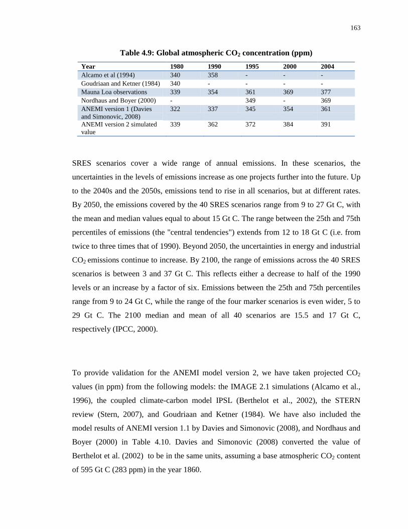
163

Table 4.9: Global atmospheric CO2 concentration (ppm)

Year 1980 1990 1995 2000 2004

Alcamo et al (1994) 340 358 - - -

Goudriaan and Ketner (1984) 340 - - - -

Mauna Loa observations 339 354 361 369 377

Nordhaus and Boyer (2000) - 349 - 369

ANEMI version 1 (Davies

and Simonovic, 2008)

322 337 345 354 361

ANEMI version 2 simulated

value

339 362 372 384 391

SRES scenarios cover a wide range of annual emissions. In these scenarios, the

uncertainties in the levels of emissions increase as one projects further into the future. Up

to the 2040s and the 2050s, emissions tend to rise in all scenarios, but at different rates.

By 2050, the emissions covered by the 40 SRES scenarios range from 9 to 27 Gt C, with

the mean and median values equal to about 15 Gt C. The range between the 25th and 75th

percentiles of emissions (the "central tendencies") extends from 12 to 18 Gt C (i.e. from

twice to three times that of 1990). Beyond 2050, the uncertainties in energy and industrial

CO2 emissions continue to increase. By 2100, the range of emissions across the 40 SRES

scenarios is between 3 and 37 Gt C. This reflects either a decrease to half of the 1990

levels or an increase by a factor of six. Emissions between the 25th and 75th percentiles

range from 9 to 24 Gt C, while the range of the four marker scenarios is even wider, 5 to

29 Gt C. The 2100 median and mean of all 40 scenarios are 15.5 and 17 Gt C,

respectively (IPCC, 2000).

To provide validation for the ANEMI model version 2, we have taken projected CO2

values (in ppm) from the following models: the IMAGE 2.1 simulations (Alcamo et al.,

1996), the coupled climate-carbon model IPSL (Berthelot et al., 2002), the STERN

review (Stern, 2007), and Goudriaan and Ketner (1984). We have also included the

model results of ANEMI version 1.1 by Davies and Simonovic (2008), and Nordhaus and

Boyer (2000) in Table 4.10. Davies and Simonovic (2008) converted the value of

Berthelot et al. (2002) to be in the same units, assuming a base atmospheric CO2 content

of 595 Gt C (283 ppm) in the year 1860.

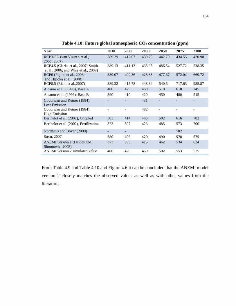
164

Table 4.10: Future global atmospheric CO2 concentration (ppm)

Year 2010 2020 2030 2050 2075 2100

RCP3-PD (van Vuuren et al.,

2006; 2007)

389.29 412.07 430.78 442.70 434.55 420.90

RCP4.5 (Clarke et al., 2007; Smith

et al., 2006; and Wise et al., 2009)

389.13 411.13 435.05 486.54 527.72 538.35

RCP6 (Fujino et al., 2006;

and Hijioka et al., 2008)

389.07 409.36 428.88 477.67 572.04 669.72

RCP8.5 (Riahi et al.,2007) 389.32 415.78 448.84 540.54 717.63 935.87

Alcamo et al. (1996), Base A 400 425 460 510 610 745

Alcamo et al. (1996), Base B 390 410 420 450 480 515

Goudriaan and Ketner (1984),

Low Emission

- - 431 - - -

Goudriaan and Ketner (1984),

High Emission

- - 482 - - -

Berthelot et al. (2002), Coupled 383 414 445 502 616 782

Berthelot et al. (2002), Fertilization 373 397 426 485 573 700

Nordhaus and Boyer (2000) - - 502

Stern, 2007 380 405 420 490 578 675

ANEMI version 1 (Davies and

Simonovic, 2008)

373 393 415 462 534 624

ANEMI version 2 simulated value 400 420 450 502 553 575

From Table 4.9 and Table 4.10 and Figure 4.6 it can be concluded that the ANEMI model

version 2 closely matches the observed values as well as with other values from the

literature.

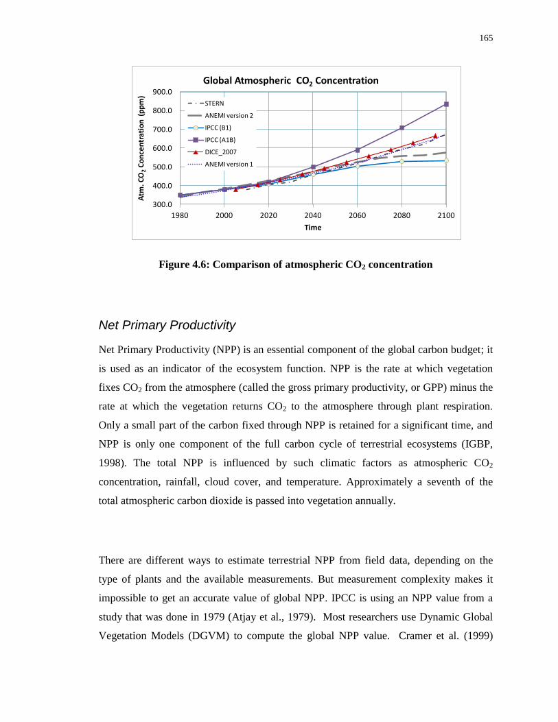
165

Figure 4.6: Comparison of atmospheric CO2 concentration

Net Primary Productivity

Net Primary Productivity (NPP) is an essential component of the global carbon budget; it

is used as an indicator of the ecosystem function. NPP is the rate at which vegetation

fixes CO2 from the atmosphere (called the gross primary productivity, or GPP) minus the

rate at which the vegetation returns CO2 to the atmosphere through plant respiration.

Only a small part of the carbon fixed through NPP is retained for a significant time, and

NPP is only one component of the full carbon cycle of terrestrial ecosystems (IGBP,

1998). The total NPP is influenced by such climatic factors as atmospheric CO2

concentration, rainfall, cloud cover, and temperature. Approximately a seventh of the

total atmospheric carbon dioxide is passed into vegetation annually.

There are different ways to estimate terrestrial NPP from field data, depending on the

type of plants and the available measurements. But measurement complexity makes it

impossible to get an accurate value of global NPP. IPCC is using an NPP value from a

study that was done in 1979 (Atjay et al., 1979). Most researchers use Dynamic Global

Vegetation Models (DGVM) to compute the global NPP value. Cramer et al. (1999)

300.0

400.0

500.0

600.0

700.0

800.0

900.0

1980 2000 2020 2040 2060 2080 2100

Atm

. CO

2C

on

cen

trat

ion

(p

pm

)

Time

Global Atmospheric CO2 Concentration

STERN

ANEMI version 2

IPCC (B1)

IPCC (A1B)

DICE_2007

ANEMI version 1

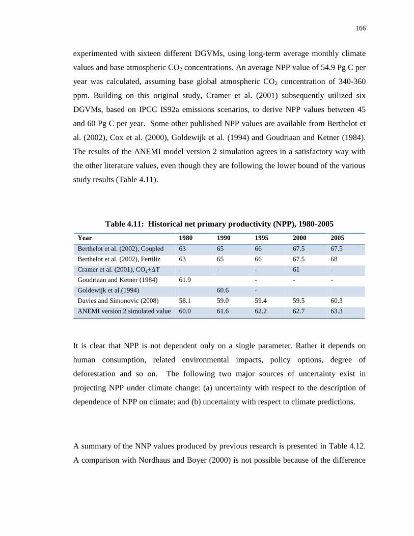
166

experimented with sixteen different DGVMs, using long-term average monthly climate

values and base atmospheric CO2 concentrations. An average NPP value of 54.9 Pg C per

year was calculated, assuming base global atmospheric CO2 concentration of 340-360

ppm. Building on this original study, Cramer et al. (2001) subsequently utilized six

DGVMs, based on IPCC IS92a emissions scenarios, to derive NPP values between 45

and 60 Pg C per year. Some other published NPP values are available from Berthelot et

al. (2002), Cox et al. (2000), Goldewijk et al. (1994) and Goudriaan and Ketner (1984).

The results of the ANEMI model version 2 simulation agrees in a satisfactory way with

the other literature values, even though they are following the lower bound of the various

study results (Table 4.11).

Table 4.11: Historical net primary productivity (NPP), 1980-2005

Year 1980 1990 1995 2000 2005

Berthelot et al. (2002), Coupled 63 65 66 67.5 67.5

Berthelot et al. (2002), Fertiliz 63 65 66 67.5 68

Cramer et al. (2001), CO2+ΔT - - - 61 -

Goudriaan and Ketner (1984) 61.9 - - -

Goldewijk et al.(1994) 60.6 -

Davies and Simonovic (2008) 58.1 59.0 59.4 59.5 60.3

ANEMI version 2 simulated value 60.0 61.6 62.2 62.7 63.3

It is clear that NPP is not dependent only on a single parameter. Rather it depends on

human consumption, related environmental impacts, policy options, degree of

deforestation and so on. The following two major sources of uncertainty exist in

projecting NPP under climate change: (a) uncertainty with respect to the description of

dependence of NPP on climate; and (b) uncertainty with respect to climate predictions.

A summary of the NNP values produced by previous research is presented in Table 4.12.

A comparison with Nordhaus and Boyer (2000) is not possible because of the difference

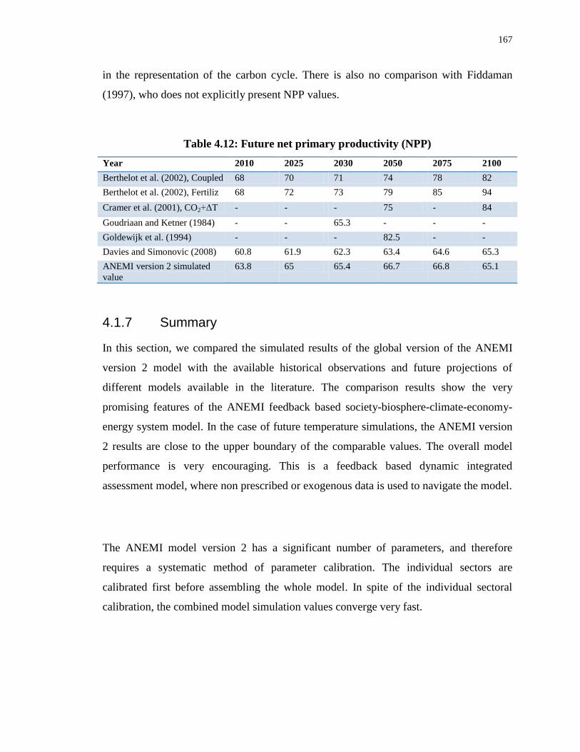
167

in the representation of the carbon cycle. There is also no comparison with Fiddaman

(1997), who does not explicitly present NPP values.

Table 4.12: Future net primary productivity (NPP)

Year 2010 2025 2030 2050 2075 2100

Berthelot et al. (2002), Coupled 68 70 71 74 78 82

Berthelot et al. (2002), Fertiliz 68 72 73 79 85 94

Cramer et al. (2001), CO2+ΔT - - - 75 - 84

Goudriaan and Ketner (1984) - - 65.3 - - -

Goldewijk et al. (1994) - - - 82.5 - -

Davies and Simonovic (2008) 60.8 61.9 62.3 63.4 64.6 65.3

ANEMI version 2 simulated

value

63.8 65 65.4 66.7 66.8 65.1

4.1.7 Summary

In this section, we compared the simulated results of the global version of the ANEMI

version 2 model with the available historical observations and future projections of

different models available in the literature. The comparison results show the very

promising features of the ANEMI feedback based society-biosphere-climate-economy-

energy system model. In the case of future temperature simulations, the ANEMI version

2 results are close to the upper boundary of the comparable values. The overall model

performance is very encouraging. This is a feedback based dynamic integrated

assessment model, where non prescribed or exogenous data is used to navigate the model.

The ANEMI model version 2 has a significant number of parameters, and therefore

requires a systematic method of parameter calibration. The individual sectors are

calibrated first before assembling the whole model. In spite of the individual sectoral

calibration, the combined model simulation values converge very fast.

168

The developed model also provides good simulation results of the system‘s future

behaviour. The satisfactory reproduction of the historical behaviour and the reasonable

future simulations together prove the model‘s robustness for use in climate change policy

analyses. We anticipate that the developed model will be able to handle different

policy/scenario analyses quite successfully, by revealing its feedback mechanism while

mimicking the near real-world system behaviour. This modelling effort is intended to

capture the system‘s future behaviour under changing climate conditions, but not to

forecast the exact magnitude of change.

4.2 ANEMI Model Version 2 Simulations

The term scenario refers to any projected course of action that is used in this research to

understand the different ways the future social-energy-economy-climate system may

come to look like. Scenario development is used in policy planning: it is a complex

process designed to test strategies against the uncertain future impact of climate change.

Therefore, scenario analysis is used to formulate flexible long-term plans by a strategic

planning method. As previously stated, the purpose of the ANEMI model is not to

forecast the future but to assist in understanding the complexity of the whole system and

to provide insight in the possible behavior of the system and its components under

changing climate conditions.

For this purpose, the ANEMI model (ANEMI version 2, ANEMI_CDN) can be used to

analyze the consequences of different policy scenarios. A given scenario may be related

to energy price, energy consumption, water use, water quality, irrigation practice,

population dynamics, land-use change or other issues. Every given issue can be addressed

by the analyses of nine model sectors.

169

While a scenario analysis does not need to be too precise, it does need to be realistic.

Accordingly, our scenarios do not attempt to represent any real situation in all its

complexity. They are always based on a variety of simplifying assumptions.

The ANEMI model (ANEMI version 2, ANEMI_CDN) provides policymakers and

scientists with a tool that can answer many ‗what if‘ questions. These partners were

engaged throughout the entire process of the model development and they provided

useful guidance and feedback. Policy dialogue was established through the consultation

sessions, workshops and direct interviews. An elaborate report on scenario development

is available in Popovich et al (2010). A detailed process of communication with the

climate change policy community (represented by the project partners) resulted in the

identification of seven policy scenarios. In the second phase of the ANEMI model

(ANEMI version 2 and ANEMI_CDN) implementation these scenarios were aggregated

into three general scenarios presented in following sections.

4.2.1 Carbon Tax Scenario

The assessment reports from the Intergovernmental Panel on Climate Change (IPCC,

2007b; Trenberth et al., 2007; Schneider et al., 2001) have identified the key potential

impacts of climate change. Furthermore, these reports point to human-induced increases

in the atmospheric concentration of greenhouse gasses (GHGs) as a likely cause of

climate change. There is a relatively strong consensus in the scientific community that

GHGs emissions need to be cut in order to reduce the impacts of climate change.

Various policy options are available to reduce GHG emissions (Popovich et al., 2010).

Three of them are tested with the ANEMI model (ANEMI version 2 and ANEMI_CDN).

The first policy to implement is a carbon tax. In the energy-economy sector, the carbon

tax is implemented as a tax per unit of CO2 emissions, effectively raising the price of

170

fossil fuel. Selected results from the carbon tax scenario are presented later in this

chapter. The carbon tax is implemented in 2012 and is slowly ramped up to $100 per

tonne of CO2 emissions over 30 years. Moreover, carbon capture and storage mechanism

is activated when carbon tax exceeds $75 per tonne of CO2 emissions from Coal. The

carbon tax has a significant impact on energy input into heat energy production as it is

primarily produced from fossil fuel. The impact on electricity production is less severe,

since the carbon tax does not impact nuclear and hydro power.

4.2.2 Increase Water Use Scenario

Water is crucial for human survival. Not only do our bodies require it; it is also a

necessary component in a growing economy. With an increasing population and rising

global temperature, the total demand for water rises irrespective of the individual water

uses (domestic, industrial and agricultural). Such an increase in water demand results in

the demand for additional infrastructure (dams, reservoirs, and diversions). Many

watersheds now have their water resources fully allocated, and greater irrigation

efficiency will be required if the total irrigated area is to expand in the future while

maintaining acceptable stream flows for other uses. Decreasing water availability,

declining water quality, and growing water demand are posing significant challenges to

human population and the health of ecosystems as well. The Intergovernmental Panel on

Climate Change (Kundzewicz et al., 2007) states that global warming will lead to

―changes in all components of the freshwater system,‖ and concludes that ―water and its

availability and quality will be the main pressures on, and issues for, societies and the

environment under climate change‘‘ (Bates et al., 2008). In areas where crops are now

receiving insufficient water for optimum growth, improved irrigation efficiencies may

actually dictate an increase in irrigation water used per unit of land. For example, in

Alberta and British Columbia, studies of irrigation system practices found that for some

crops, producers were under-irrigating and could improve production by increasing the

amount of water applied. At the same time, continued improvement in irrigation and

conveyance efficiency will free up some water for other uses.

171

Climate change projections for Canada indicate a 37% increase in irrigation water

demand in the Okanagan Valley, B.C. (Neilsen et al., 2001). In addition, global warming

may necessitate an increase in crop irrigation in the Prairies, Ontario, Quebec and the

Atlantic Provinces as well. Therefore, the second policy scenario included in this research

focuses on increased water use. The ANEMI model thus tested an assumed amount of

15% increase across all water uses.

4.2.3 Food Production Increase Scenario

In a recent news release, the Food and Agriculture Organization of the United Nations

stated that ―Producing 70 percent more food for an additional 2.3 billion people by 2050

while at the same time combating poverty and hunger, using scarce natural resources

more efficiently and adapting to climate change are the main challenges world agriculture

will face in the coming decades‖ (FAO, 2009).

This scenario is closely related to the previous one, in which the demand for water is

expected to increase. Whereas the water usage scenario experiments with the impact of

increasing irrigation to cope with rising food demand, the food production scenario tests

the impact of redistributing land-use, by converting more land from forest to agriculture.

It also uses both global and regional versions of the ANEMI model (ANEMI version 2,

ANEMI_CDN), drawing a broader set of conclusions regarding the world‘s capacity to

meet global food demand. Finally, the scenario also shows the sink capacity of the land,

and produces output in various sectors—namely, population, hydrologic cycle, water

quality, energy-economy, climate, carbon, and food production.

172

4.3 Global ANEMI Model (Version 2) Analyses Results

The following three sections present the main results of ANEMI version 2 simulations of

the three policy scenarios introduced above.

4.3.1 Global Carbon Tax Scenario

The carbon tax is implemented in 2012 and slowly ramped up to $100 per tonne of CO2

over 30 years. Figure 4.7 and Figure 4.8 show how the implementation of the carbon tax

affects electric and heat energy production. The dashed line in these two figures shows

the ANEMI version 2 simulation results without the carbon tax, and the full line shows

the results with the carbon tax in place. The carbon tax has a significant impact on heat

energy production, which relies on fossil fuel as an energy input. However, the carbon

tax has less of an effect on electricity production, which rather relies on nuclear and

hydro power.

Figure 4.7: Energy used to produce electricity

0

1

2

3

4

5

6

1980 2000 2020 2040 2060 2080 2100

10

11

GJ

Time

Energy Used for Electricity Production

Base

With Tax

173

Figure 4.8: Energy used to produce heat energy

The implemented carbon-tax policy restricts the amount of carbon emissions in the

production of each unit amount of energy. This creates significant pressure on fossil fuel

pricing. Following the elasticity of substitution, the share of each fossil fuel type is

automatically adjusted to produce low cost energy. The result is not only the production

of cost effective energy via a certain combination of coal, oil and natural gas. More

importantly, there is a dramatic drop in energy consumption that changes the whole

dynamics of the global energy-economy sector (Figure 4.9). An initial reduction of fossil

fuel based energy consumption immediately follows the implementation of the carbon-

tax, and this helps to maintain a relatively stable supply of fossil fuel based energy

throughout the 21st century. Such behaviour is driven by the availability of the fossil fuel

reserve. In the base simulation, fossil fuel prices started to climb up as the reserves

started to decline, and by 2080 the world had mostly run out of fossil fuel to produce heat

and electric energy. Under the carbon tax scenario, however, the initial reduction in

energy consumption saves a significant portion of fossil fuel to burn later. As the fossil

fuel based energy consumption decreases significantly, so the fossil fuel based emissions

0

1

2

3

4

5

6

1980 2000 2020 2040 2060 2080 2100

10

11

GJ

Time

Energy Used for Heat Energy Production

With Tax

Base

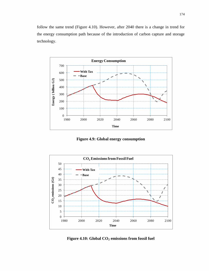
174

follow the same trend (Figure 4.10). However, after 2040 there is a change in trend for

the energy consumption path because of the introduction of carbon capture and storage

technology.

Figure 4.9: Global energy consumption

Figure 4.10: Global CO2 emissions from fossil fuel

0

100

200

300

400

500

600

700

1980 2000 2020 2040 2060 2080 2100

En

erg

y (

bil

lio

n G

J)

Time

Energy Consumption

With Tax

Base

0

5

10

15

20

25

30

35

40

45

50

1980 2000 2020 2040 2060 2080 2100

CO

2em

issi

on

s (G

t)

Time

CO2 Emissions from Fossil Fuel

With Tax

Base

175

The main source of anthropogenic emissions is the burning of fossil fuel and forest

cutting/burning. Under this scenario, fossil fuel based emissions are reduced by almost

half, significantly lowering the atmospheric CO2 concentration increment rate. By 2100,

the global atmospheric concentration could thus be well below 500ppm (Figure 4.11).

Atmospheric CO2 concentration is considered as one of the sources of increased radiative

forcing; that is, it works as a driving force for the increase in global temperature. The

model also shows a drop of around 0.5 0C in atmospheric temperature by 2100, compared

to the base condition (Figure 4.12). Due to its positive correlation, the sea-level rising

rate slows down relative to the base run with no carbon tax (Figure 4.13).

Figure 4.11: Global atmospheric CO2 concentration

300

350

400

450

500

550

600

1980 2000 2020 2040 2060 2080 2100

CO

2co

nce

ntr

ati

on

(p

pm

)

Time

Atmospheric CO2 Concentration

With Tax

Base

176

Figure 4.12: Global atmospheric temperature change

Figure 4.13: Global sea-level rise

Following the implementation of the carbon tax policy, the suitable temperature and

decreased pollution result in an increase in human life expectancy. The global population

14.0

14.5

15.0

15.5

16.0

16.5

17.0

17.5

1980 2000 2020 2040 2060 2080 2100

Tem

per

atu

re (

0C

)

Time

Atmospheric Temperature

With Tax

Base

0

30

60

90

120

150

1980 2000 2020 2040 2060 2080 2100

Sea

-lev

el r

ise(

mm

)

Time

Sea-Level Rise

With Tax

Base

177

thus increases by almost 10% over the following 50 years in comparison to the base

condition (Figure 4.14). This population increase demands more food production (Figure

4.15), and this leads to a higher water demand for irrigation. As more irrigation produces

higher water pollution, the water-stress starts to increase as more fresh water is required

for dilution (Figure 4.16). This eventually acts as a negative feedback force in the food

production and population sectors. The global GDP also exhibits 13% increase from the

base conditions in 2100 (Figure 4.17).

Figure 4.14: Global population

4

5

6

7

8

9

10

11

12

13

14

1980 2000 2020 2040 2060 2080 2100

Po

pu

lati

on

(B

illi

on

)

Time

Global Population

With Tax

Base

178

Figure 4.15: Global food production

Figure 4.16: Global water-stress

0

4000

8000

12000

16000

20000

1980 2000 2020 2040 2060 2080 2100

Fo

od

(tr

illi

on

kil

oca

lori

e/y

r)

Time

Food Production

With Tax

Base

0.30

0.35

0.40

0.45

0.50

0.55

0.60

0.65

0.70

1980 2000 2020 2040 2060 2080 2100

Wa

ter

Str

ess(

dim

ensi

on

less

)

Time

Water Stress

With Tax

Base

179

Figure 4.17: Global GDP change

The impact of the carbon tax on GDP per capita is the first negative (albeit minor)

impact, because of the distortion created by the tax policy (Figure 4.17). Eventually all

the benefits from the reduction of climate damage and the price effects for fossil fuel

suppress the tax distortion effect. As stated above, the price effect for fossil fuel shows

some benefit in delaying the depletion of the reserves. In the ANEMI model version 2,

fossil fuel prices are a function of the reserve level relative to the base year. That is, when

reserves decrease, the price starts to increase, and the benefits from delaying the price

increase are significant.

4.3.2 Global Water Use Scenario

The ANEMI model version 2 tested a second scenario involving a 15% increase in water

use throughout the domestic, industrial and agricultural sectors. The intention of this

scenario is not to forecast the future, but to identify the probable impacts of increased

water use on other sectors of the model and find how the multiple feedbacks determine

the system response.

0

100

200

300

400

500

1980 2000 2020 2040 2060 2080 2100

GD

P (

tril

lio

n $

)

Time

GDP

With Tax

Base

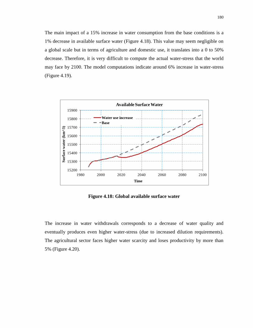
180

The main impact of a 15% increase in water consumption from the base conditions is a

1% decrease in available surface water (Figure 4.18). This value may seem negligible on

a global scale but in terms of agriculture and domestic use, it translates into a 0 to 50%

decrease. Therefore, it is very difficult to compute the actual water-stress that the world

may face by 2100. The model computations indicate around 6% increase in water-stress

(Figure 4.19).

Figure 4.18: Global available surface water

The increase in water withdrawals corresponds to a decrease of water quality and

eventually produces even higher water-stress (due to increased dilution requirements).

The agricultural sector faces higher water scarcity and loses productivity by more than

5% (Figure 4.20).

15200

15300

15400

15500

15600

15700

15800

15900

1980 2000 2020 2040 2060 2080 2100

Su

rfa

ce w

ate

r (k

m^

3)

Time

Available Surface Water

Water use increase

Base

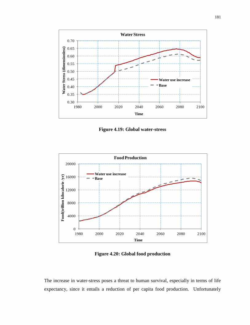
181

Figure 4.19: Global water-stress

Figure 4.20: Global food production

The increase in water-stress poses a threat to human survival, especially in terms of life

expectancy, since it entails a reduction of per capita food production. Unfortunately

0.30

0.35

0.40

0.45

0.50

0.55

0.60

0.65

0.70

1980 2000 2020 2040 2060 2080 2100

Wa

ter

Str

ess

(dim

ensi

on

less

)

Time

Water Stress

Water use increase

Base

0

4000

8000

12000

16000

20000

1980 2000 2020 2040 2060 2080 2100

Fo

od

(tri

llio

n k

ilo

calo

rie

/yr)

Time

Food Production

Water use increase

Base

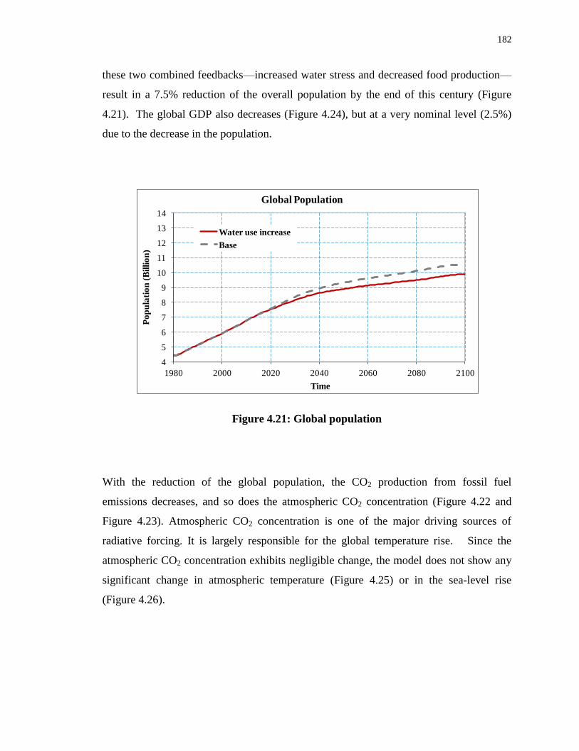
182

these two combined feedbacks—increased water stress and decreased food production—

result in a 7.5% reduction of the overall population by the end of this century (Figure

4.21). The global GDP also decreases (Figure 4.24), but at a very nominal level (2.5%)

due to the decrease in the population.

Figure 4.21: Global population

With the reduction of the global population, the CO2 production from fossil fuel

emissions decreases, and so does the atmospheric CO2 concentration (Figure 4.22 and

Figure 4.23). Atmospheric CO2 concentration is one of the major driving sources of

radiative forcing. It is largely responsible for the global temperature rise. Since the

atmospheric CO2 concentration exhibits negligible change, the model does not show any

significant change in atmospheric temperature (Figure 4.25) or in the sea-level rise

(Figure 4.26).

4

5

6

7

8

9

10

11

12

13

14

1980 2000 2020 2040 2060 2080 2100

Po

pu

lati

on

(B

illi

on

)

Time

Global Population

Water use increase

Base

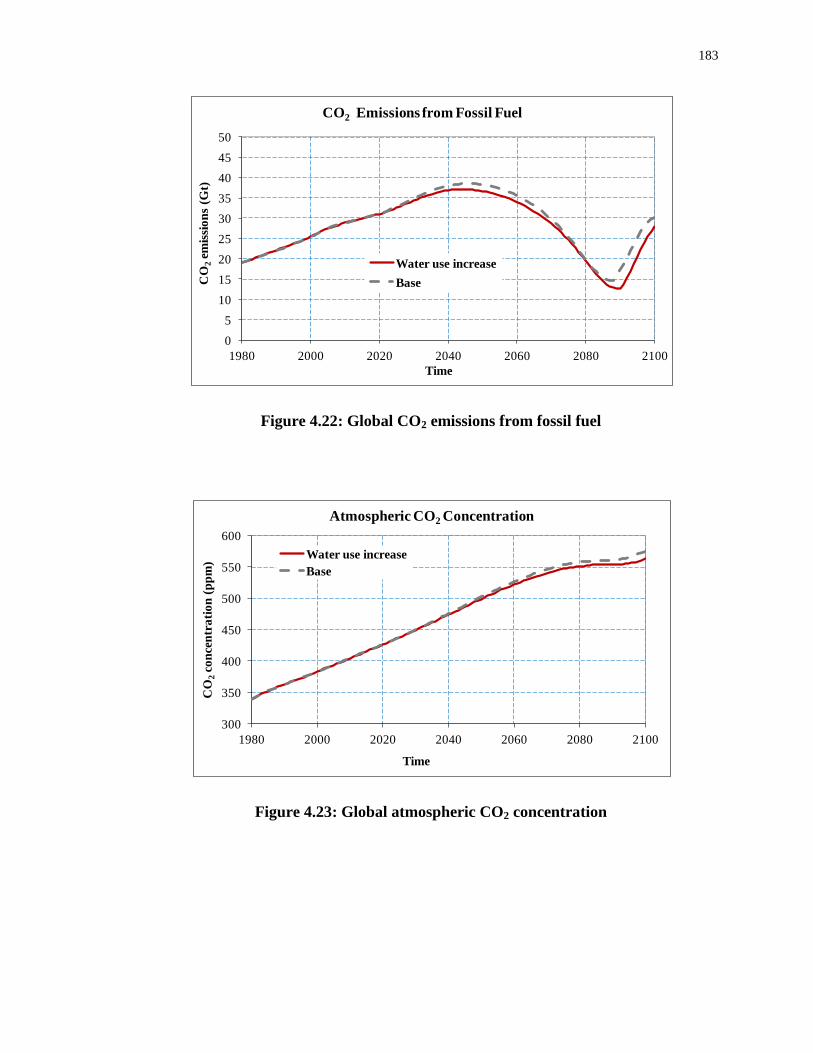
183

Figure 4.22: Global CO2 emissions from fossil fuel

Figure 4.23: Global atmospheric CO2 concentration

0

5

10

15

20

25

30

35

40

45

50

1980 2000 2020 2040 2060 2080 2100

CO

2em

issi

on

s (G

t)

Time

CO2 Emissions from Fossil Fuel

Water use increase

Base

300

350

400

450

500

550

600

1980 2000 2020 2040 2060 2080 2100

CO

2co

nce

ntr

ati

on

(p

pm

)

Time

Atmospheric CO2 Concentration

Water use increase

Base

184

Figure 4.24: Global GDP

Figure 4.25: Global atmospheric temperature

0

100

200

300

400

500

1980 2000 2020 2040 2060 2080 2100

GD

P (

tril

lio

n $

)

Time

GDP

Water use increase

Base

14.0

14.5

15.0

15.5

16.0

16.5

17.0

17.5

1980 2000 2020 2040 2060 2080 2100

Tem

per

atu

re (

0C

)

Time

Atmospheric Temperature

Water use increase

Base

185

Figure 4.26: Global sea-level rise

4.3.3 Global Food Production Scenario

The simulations of the third scenario attempt to determine how an increase in agricultural

land will affect global food production. In the ANEMI model version 2, the land

conversion rate (from forest to agriculture) is increased by 15% to allow for an increase

in food production. This will also allow the model to identify the probable impacts on

other sectors. For this investigation, we analyze such important parameters and variables

as food production, available surface water, water-stress, global population, and CO2

concentration.

The simulation results (Figure 4.27) demonstrate that a 15% increase in agricultural land

conversion results in a 1% increase in food production at the beginning of the policy

implementation period. However, the extra production slowly starts to decline because of

the water shortage. Moreover, after 2090, the total food production ultimately falls below

the base conditions (no increase in land conversion) (Figure 4.27).

0

30

60

90

120

150

1980 2000 2020 2040 2060 2080 2100

Sea

-lev

el r

ise(

mm

)

Time

Sea-Level Rise

Water use increase

Base

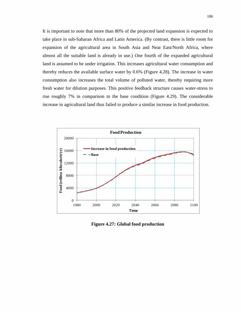
186

It is important to note that more than 80% of the projected land expansion is expected to

take place in sub-Saharan Africa and Latin America. (By contrast, there is little room for

expansion of the agricultural area in South Asia and Near East/North Africa, where

almost all the suitable land is already in use.) One fourth of the expanded agricultural

land is assumed to be under irrigation. This increases agricultural water consumption and

thereby reduces the available surface water by 0.6% (Figure 4.28). The increase in water

consumption also increases the total volume of polluted water, thereby requiring more

fresh water for dilution purposes. This positive feedback structure causes water-stress to

rise roughly 7% in comparison to the base condition (Figure 4.29). The considerable

increase in agricultural land thus failed to produce a similar increase in food production.

Figure 4.27: Global food production

0

4000

8000

12000

16000

20000

1980 2000 2020 2040 2060 2080 2100

Fo

od

(tr

illi

on

kil

oca

lori

e/y

r)

Time

Food Production

Increase in food production

Base

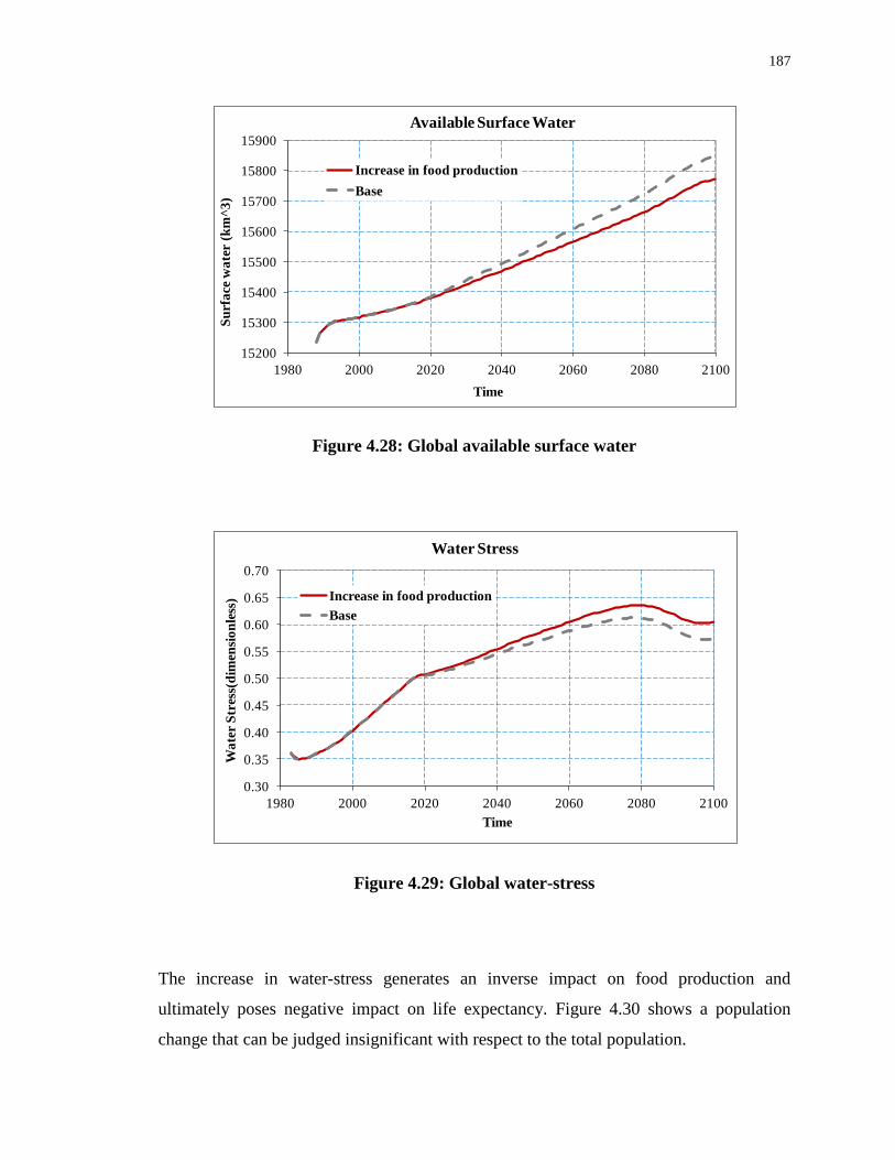
187

Figure 4.28: Global available surface water

Figure 4.29: Global water-stress

The increase in water-stress generates an inverse impact on food production and

ultimately poses negative impact on life expectancy. Figure 4.30 shows a population

change that can be judged insignificant with respect to the total population.

15200

15300

15400

15500

15600

15700

15800

15900

1980 2000 2020 2040 2060 2080 2100

Su

rfa

ce w

ate

r (k

m^

3)

Time

Available Surface Water

Increase in food production

Base

0.30

0.35

0.40

0.45

0.50

0.55

0.60

0.65

0.70

1980 2000 2020 2040 2060 2080 2100

Wa

ter

Str

ess(

dim

ensi

on

less

)

Time

Water Stress

Increase in food production

Base

188

Figure 4.30: Global population

CO2 emissions from fossil fuel and GDP are directly related to the population. The

simulated results show very small changes in this case (Figure 4.31 and Figure 4.32).

However, the model results show a nearly 1% increase in global CO2 concentration

(Figure 4.33). This may be a significant finding. In reality, the atmospheric concentration

of CO2 does not originate solely in fossil fuel burning. A significant portion of carbon

also comes from changes in land-use. In this simulation, the extra amount of atmospheric

CO2 concentration is the consequence of 15% increase in land conversion (specifically

forest cutting/burning) to expand the agricultural land.

4

5

6

7

8

9

10

11

12

13

14

1980 2000 2020 2040 2060 2080 2100

Po

pu

lati

on

(B

illi

on

)

Time

Global Population

Increase in food production

Base

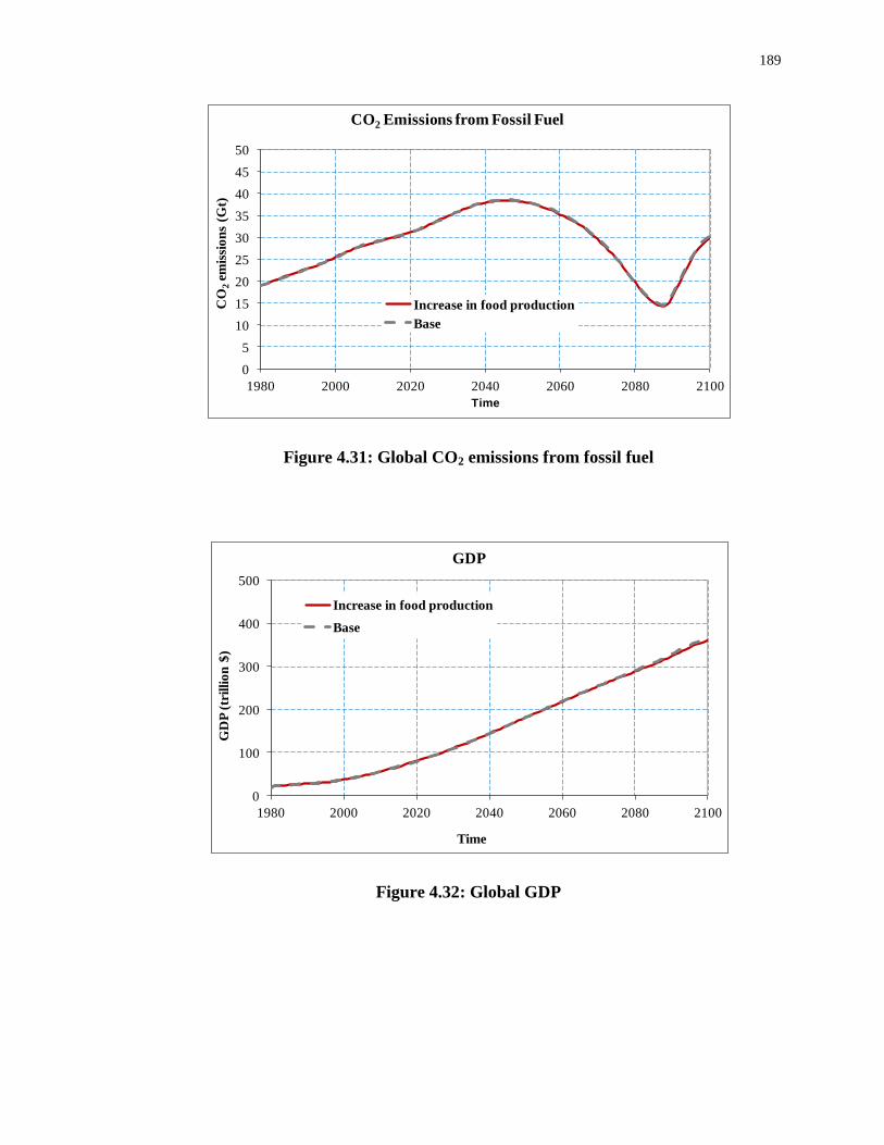
189

Figure 4.31: Global CO2 emissions from fossil fuel

Figure 4.32: Global GDP

0

5

10

15

20

25

30

35

40

45

50

1980 2000 2020 2040 2060 2080 2100

CO

2em

issi

on

s (G

t)

Time

CO2 Emissions from Fossil Fuel

Increase in food production

Base

0

100

200

300

400

500

1980 2000 2020 2040 2060 2080 2100

GD

P (

tril

lio

n $

)

Time

GDP

Increase in food production

Base

190

Figure 4.33: Global atmospheric CO2 concentration

A minor change in atmospheric CO2 concentration contributes to a small increase in

radiative forcing that affects the global temperature change (Figure 4.34). As the forcing

from solar radiation and other gases remain unchanged, the effect of only 1% increases in

CO2 concentration dampens further. Since sea-level change is only a function of

temperature, the model produces the same trend for sea-level change (Figure 4.35).

300

350

400

450

500

550

600

1980 2000 2020 2040 2060 2080 2100

CO

2co

nce

ntr

ati

on

(p

pm

)

Time

Atmospheric CO2 Concentration

Increase in food production

Base

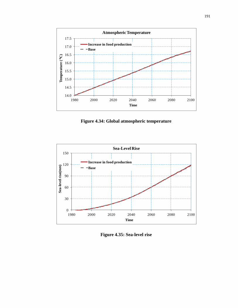
191

Figure 4.34: Global atmospheric temperature

Figure 4.35: Sea-level rise

14.0

14.5

15.0

15.5

16.0

16.5

17.0

17.5

1980 2000 2020 2040 2060 2080 2100

Tem

per

atu

re (

0C

)

Time

Atmospheric Temperature

Increase in food production

Base

0

30

60

90

120

150

1980 2000 2020 2040 2060 2080 2100

Sea

-lev

elri

se(m

m)

Time

Sea-Level Rise

Increase in food production

Base

192

CHAPTER 5

5 REGIONAL MODEL OF THE SOCIAL-ENERGY-ECONOMY-CLIMATE SYSTEM

Using a system dynamics simulation approach, the ANEMI model combines simplified

representations of the socioeconomic determinants of greenhouse gas emissions with

representations of the atmosphere and oceans in order to determine the global impact of

human activities on the Earth‘s ecosystem. Version 2 of ANEMI model has nine major

sectors, all of which interact with one another through feedback relationships. With

respect to its global scale, the ANEMI model version 2 shares important characteristics

with other climate-economy models, integrated assessment models and hydrologic

models.

The major limitation of the ANEMI model version 1 is that it cannot model on a regional

or local scale. In order to develop suitable mitigation strategies for different regions of

the world, a model must be able to describe regional and local impacts of climate change.

This requires an appropriate degree of spatial resolution. A model cannot attain this

degree of resolution if it can only represent globally. Hence the second objective of the

work presented in this thesis has been the regionalization of the global ANEMI model

version 2.

The regionalization of the ANEMI model is important because it allows modelers and

policy makers to investigate the effects of global climate change on regional water

resources, energy supply and demand, population and land-use, and economic

performance. Hence the regional model allows policy makers to assess regional policy

options for stabilizing global climate.

193

With the ANEMI version 2, we chose Canada as the particular regional emphasis. This

regional ANEMI model (ANEMI_CDN) thus separates Canada from the rest of the world

(ROW). As the climate, carbon and a portion of the hydrologic cycle related sectors deal

with global processes, they have remained on a global scale.

There are two different approaches that can be used for downscaling a global model to a

regional scale: bottom-up and top-down. The typical bottom-up approach focuses on

individual sectors, not on the relationships within the combined system. Therefore, the

implementation of such a model is relatively simple. The top-down modelling approach

considers the system as a whole, irrespective of the number of sectors and subsectors. It

thus counts different inputs across the model domain. For the regionalization of the

ANEMI model version 2, we took the top-down approach.

The following sections provide detailed explanations of the structure of each regionalized

sector. The regionalized sectors include 1) population, 2) land-use, 3) hydrologic cycle,

4) water demand, 5) water quality, 6) food production, and 7) energy-economy. This

presentation of the regional model (ANEMI_CDN) focuses only on the main concepts

and feedbacks. The rest of the details are already provided in the global model

description. However, we must also address the matter of the integration of the global

sectors with the regionalized ones. Hence we also provide a presentation of the

disaggregation procedure that we implemented for this purpose.

194

5.1 Description of Individual Sectors of the ANEMI_CDN Model

5.1.1 The Population Sector

The population sector represents the growth or decline of regional population under the

influence of other sectors. The population change is derived from birth rate, death rate,

and migration. In this model, death rate is influenced my extreme temperature and life

expectancy is affected by water-stress, per capita food production, and pollution. GDP,

which is the output of the energy-economy sector, plays a significant role by allocating

the required amount of funding to the family planning services.

The simulations of the regional ANEMI model (ANEMI_CDN) start from 1980, and thus

we required the initial regional distribution of the global population. We obtained this

regional value from the UN population data for 1980 (DESA, 2011). We based the

calculations of the initial population growth rates for the two ANEMI model regions,

Canada and ROW, on the population growth from 1975 to 1980.

The regionalized population sector simulates population distribution that matches UN

predictions up to 2050. International migration (between Canada and ROW) is also

incorporated in the ANEMI_CDN model, since the population migrating to Canada

constitutes a vital source of labour force. (The model also has the capability of handling

the environmental refugee/migration inflow based on the Canadian immigration policy.)

The structure for the population sector in the ANEMI_CDN model is exactly the same as

that of the global model. (See section 3.1.6). Hence the same governing equations and

195

most of the parameter values are valid for both versions of the model. The initial values

of the population in 1980 are shown in Table 5.1.

Table 5.1: Population by age-group of 1980 (DESA, 2011)

Age group (year) 0-14 15-44 45-64 65 to 65+

Canada (population in millions) 5.575 12.00 4.637 2.305

Rest of the world (population in millions) 1560 1940 6520 259

5.1.2 The Land-Use Sector

The land-use sector is highly influenced by the population sector. In other words, the land

transfer rate is proportional to population growth. Forest clearing and burning activities

thus reflect the demands of a growing population. Land-use policies reflect an awareness

of this relationship, as well as an awareness of various other environmental issues. In this

model, however, population growth is taken as the lone variable that affects changes in

existing land-use patterns.

Since population is taken as the main determining factor in land-use, the ANEMI_CDN

requires the regionalization of the land transfer matrix. The regional transfer matrix is

derived from the global value (provided by Goudrian and Ketner, 1994) and the available

land area for each region. In the regionalization of the land-use sector, the simple

assumption is thus that the land transformation rate is only the function of the given

region‘s total land area. Admittedly, this type of regionalization has its setbacks, as the

data limitation at the regional scale introduces uncertainty into the land transfer matrix.

However, the reduction in uncertainty can be obtained through multiple attempts at

calibrating the model output.

196

In the ANEMI_CDN, the land-use model structure and parameter values remain

unchanged from the global model (as presented in section 3.1.5), with the exception of

the initial transfer matrix (given in Table 5.2). This matrix is calculated based on the ratio

of land area of Canada and the rest of the world. The land transfer matrix for the ROW is

thus obtained by deducting the land transfer value in Table 5.2 from the value in Table

3.5.

Table 5.2: Initial land transfer matrix for Canada (Mha yr-1

, in 1980)

From( j):

To (i):

Tropical

Forest

Temperate

Forest

Grassland Agricultural

Land

Human

Area

Semi-

Desert and

Tundra

Tropical Forest 0 0 0 0 0 0

Temperate Forest 0 0.814148 0 0 0 0

Grassland 0 0.05 21.7106 0 0 0

Agricultural Land 0 0.12 0 21.7106 0 0.015

Human Area 0 0.01 0.04828 0.04828 0 0

Semi-Desert and

Tundra

0 0 0 0 0 0

5.1.3 The Water Sectors

One of the main strengths of the ANEMI model is the presence of three water sectors that

(a) link climate change with other socio-economic sectors and (b) provide for the

assessment of impacts caused by water deficiency and water quality degradation on

population, industrial output and food production. The three major water sectors that the

ANEMI model incorporates to deal with global and regional water resources are (a) the

hydrologic cycle, (b) water demand, and (c) water quality.

5.1.3.1 Hydrologic Cycle

The sector represents the hydrologic cycle describes the interactions among land, water

and atmosphere. The sector‘s objective is to estimate the balance between water supply

and water demand within a given region, and to determine the effects of water deficiency

197

on other sectors. The current version of the ANEMI_CDN model is not well equipped to

address the effects of excess water (flooding) on the other socio-economic sectors.

The atmospheric and oceanic portions of the hydrologic cycle are the same as in the

global version of the model. Only precipitation is regionalized. In other words, the

regionalization of this sector is not able to produce regional atmospheric water content,

but it is definitely able to disaggregate regional discharge and surface water availability

through long term observations of rainfall and land characteristics. As one cannot

separate the atmospheric water content and temperature of Canada from ROW, one must

perform the disaggregation based on the historical data. The rainfall and temperature are

disaggregated using outputs of 17 GCM models (see section 5.3). However, the

ANEMI_CDN model is not able to capture the expected shifting of global rainfall

patterns at a desirable spatial resolution.

5.1.3.2 Water Demand

Industrial use, agricultural use and municipal use comprise the main sources of water

demand. Thus, the population, energy-economy and hydrologic cycle sectors each

contribute to the factors of water demand, consumption, water use intensity, water

quality, wastewater treatment and water availability.

The regionalization of the water demand sector is carried out in a simple way. In regions

where water is a scarce resource, waste-water treatment and desalination capacity play

important roles in the water demand sector. The regional distribution of the desalinated

water supply capacity for ROW is obtained from the World‘s Water 2006-2007 (Pacific

Institute, 2007). While distributing the capacity, we consider only those countries/regions

that possess more than one percent of the world‘s desalination capacity. Waste water

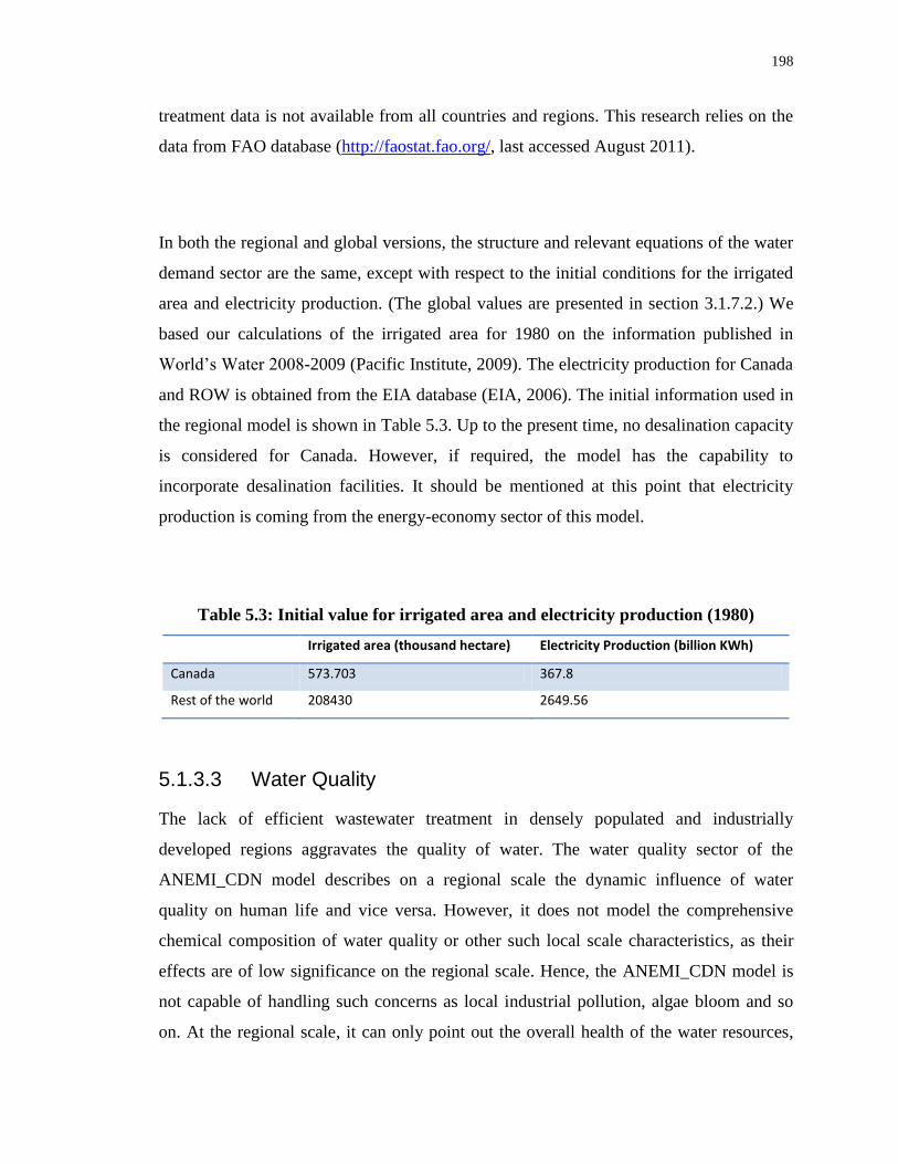
198

treatment data is not available from all countries and regions. This research relies on the

data from FAO database (http://faostat.fao.org/, last accessed August 2011).

In both the regional and global versions, the structure and relevant equations of the water

demand sector are the same, except with respect to the initial conditions for the irrigated

area and electricity production. (The global values are presented in section 3.1.7.2.) We

based our calculations of the irrigated area for 1980 on the information published in

World‘s Water 2008-2009 (Pacific Institute, 2009). The electricity production for Canada

and ROW is obtained from the EIA database (EIA, 2006). The initial information used in

the regional model is shown in Table 5.3. Up to the present time, no desalination capacity

is considered for Canada. However, if required, the model has the capability to

incorporate desalination facilities. It should be mentioned at this point that electricity

production is coming from the energy-economy sector of this model.

Table 5.3: Initial value for irrigated area and electricity production (1980)

Irrigated area (thousand hectare) Electricity Production (billion KWh)

Canada 573.703 367.8

Rest of the world 208430 2649.56

5.1.3.3 Water Quality

The lack of efficient wastewater treatment in densely populated and industrially

developed regions aggravates the quality of water. The water quality sector of the

ANEMI_CDN model describes on a regional scale the dynamic influence of water

quality on human life and vice versa. However, it does not model the comprehensive

chemical composition of water quality or other such local scale characteristics, as their

effects are of low significance on the regional scale. Hence, the ANEMI_CDN model is

not capable of handling such concerns as local industrial pollution, algae bloom and so

on. At the regional scale, it can only point out the overall health of the water resources,

199

including the availability of sufficient water supply for human survival within the ‗water-

stress‘ parameter. In general the ‗water quality‘ sector concerns itself with the necessary

requirements that a region must fulfill in order to maintain standard water quality. A good

example of such requirements is fresh water dilution.

The water quality sector is connected with the water demand sector by negative causal

relationship. Domestic, industrial and agricultural wastewater values thus serve as

components of the sector. The initial irrigated area for each region (Canada and ROW in

1980) is calculated from the World Bank online database

(http://databank.worldbank.org/, last accessed August 2011).

The structure of the ANEMI_CDN model water quality sector remains the same as the

global model (See section 3.1.7.3.). In the regional model, most of the parameter values

also remain the same as those of the global model, except for the initial treatment

percentage. The assumed initial values for Canada are 55% for domestic waste and 65%

industrial waste. To derive these values, we took the simulated global results of the

ANEMI version 1.2 for the year 1980 and increased them by 20% to represent Canada.

We assumed that, as a first world country, Canada would have more treatment facilities

than the global average. Such an assumption is supported by Environment Canada‘s

statement that ―As of 1994, 81% of Canadians were served by some level of treatment,

whereas < 56% of Canadians were served in 1980‖ (EC, 2008). The values for the ‗rest

of the world‘ are the same as in the global model of ANEMI version 1.2: 35% for

domestic waste and 45% for industrial waste.

5.1.4 The Food Production Sector

The food production sector of the regional ANEMI model (ANEMI_CDN) is connected

to a large number of other sectors, making it more interactive and complex. And yet the

200

regionalization of this sector is not very complex, since most of the inputs that it obtains

from other sectors are already regional values. Its structure therefore remains the same as

that of its global counterpart (presented in section 3.1.4), and the parameter values that it

obtains from connected sectors determine its behaviour. Other initial stocks such as the

‗initial total erodible land‘ do not require regionalization. They start with zero value.

5.1.5 The Energy-Economy Sector

The energy-economy sector of the ANEMI_CDN model takes into account both Canada

and ROW. As a region, Canada is considered a small open economy that takes energy

prices and the global mean temperature as given. In other words, fossil fuel prices and the

global mean temperature are exogenous to the region‘s energy-economy sector.

Conversely, they are endogenous variables in the ROW region.

It is assumed that energy consumption and energy based CO2 emissions in the Canada

region do not significantly impact the world, since Canada contributes about 2% of total

global greenhouse gas emissions (calculated from WDI database, last accessed November

2011). The structure of the Canada region is almost identical to the global energy

economy sector. The main difference is that the regional energy economy allows for a

simple representation of trade in fossil fuels.

In the regional energy-economy sector, extraction decisions are based on the fossil fuel

price functions of the global version of the ANEMI (ANEMI version 2) model‘s energy

sector. As we presume the price of fossil fuel to be exogenous to Canada, the desired

amount of fossil fuel to extract is obtained through the inverse of the price functions:

201

where is the total extraction of fossil fuel type at time , given the current world

price

. is the current reserve value, is the reserve value at the base year,

is new discoveries, and is the world price of fossil fuel at the base year.

is an elasticity parameter, and is a calibration parameter adjusting the level of

extraction.

It is assumed that the difference between demand and total extraction each period yields

the net exports of fossil fuel i, , is the difference between demand and total

extraction each period. That is, the net exports of fossil fuel type i equal the total

extraction minus the fuel used for the production of heat and electric energy:

The structure for the production of energy in the regional model is exactly the same as in

the global model. (See section 3.1.3.) The regional model thus uses the same production

functions for heat energy and electricity production, and the aggregation into total energy

services.

The demand for fossil fuels is derived in relation to their exogenous world price. Since

the price for fossil fuels is exogenous, there is no mechanism to clear the market for fossil

fuels in the regional energy-economy sector. Demand and supply are determined

202

separately. If supply is greater than demand, the excess is exported. Conversely, if

demand is greater than supply, the excess is imported.

In the regional model of ANEMI (ANEMI_CDN), many of the parameter values for the

production functions of energy and energy aggregation are the same as in the global

model. However, some differences occur in the reserve values, the discoveries of fossil

fuel sources and the price functions for fossil fuel sources. The assumed future discovery

of fossil fuels in Canada is presented in Table 5.4.

Table 5.4: Assumed future fossil fuel discovery (Canada) in billion GJ

1980

Assumed Initial

Reserves

1980 Reserves

(EIA & Statistics

Canada)

1980-2005

Discoveries (EIA &

Statistics Canada)

2006 -

Assumed

Discoveries

Coal 140 90 50 -

Oil 2500 40 1180 1280

Natural Gas 400 77 133 190

Canada has a vast reserve of oil sands. But economic, political, and technological

constraints make it very difficult to predict what share of the oil sands will actually be

extracted. In 2007, for example, the Alberta Energy and Utilities Board estimated that

with the then current economic conditions and technological restraints about 10% of the

oil was recoverable. Given such constraints, we make the assumption that the total

recoverable oil in Canada is about 410 billion barrels, approximately 25% of the oil

estimated to be in the Alberta‘s oil sands (conversion factor from the EIA is 1 barrel of

oil = 6.119 GJ). We make a similar assumption about natural gas: discovery and

extraction depend upon technological improvements and the increase in price.

203

5.2 Disaggregation Procedure

Climate change processes take place over various temporal and spatial scales. One of the

main requirements of an integrated assessment model is to model the various impacts of a

given process across different scales. And nowadays, one of the main methods to assist

in the transference of information across scales is disaggregation. Harms and Campbell

(1967) were among the first researchers to formalize the disaggregation approach and

apply it to the temporal disaggregation of streamflow. Lane (1979) was among the first to

transfer the same disaggregation principles into the spatial domain. The regionalization of

the ANEMI model requires the disaggregation of spatial and temporal information. The

implemented procedures are described in the following sections.

5.2.1 Temporal Disaggregation

The main objective of any disaggregation technique is to maintain the statistical

properties of a given set of data at more than one level. For example, disaggregation

maintains the statistical properties of annual streamflow data as it generates monthly

streamflow data for water resources management purposes. Desirable statistical

properties in this type of disaggregation approach can include mean, variances,

probability distribution and covariance. Disaggregation can also reduce the parameters of

a generated set of data with little or no corresponding loss of its desirable properties.

Disaggregation is more complex than such basic time series approaches as autoregressive

(AR) modelling. Hence its application is more difficult. However, the disaggregation

process eliminates many common problems that practitioners encounter with

stochastically generated data. The added benefits make the required effort worthwhile

(Salas et al., 2009).

204

The disaggregation process generates new time series out of a previously established data

series. The generation of a disaggregated series (for example, monthly or daily data from

annual data) may be done with the help of a linear model that functions to preserve

important statistical properties of the original series. Disaggregation can be implemented

in time and space.

In general all disaggregation models can be articulated in terms of a linear dependence

model as:

where is the current observation of the time series that will be generated, is the

original series or independent series, ε represents the current value from a completely

random series (stochastic term). and are matrices of parameters.

It should be noted that in this approach each of the time series that make up and must

follow the normal distribution with zero mean. This condition could be secured by taking

the original data series and transforming the individual values to normally distributed

values and then subtracting the mean from the transformed values. The stochastic terms

in matrix ε are assumed to be normal with zero mean and a variance of one. The

advantage of this disaggregation model is its very clean structure.

Mejia et al. (1976) introduced the following form of temporal disaggregation procedure:

205

where is a parameter matrix with the same dimensions as , is a column matrix

containing monthly values from the previous year.

From the above equation, Lane (1979) developed a condensed form of disaggregation

model, where numbers of parameters are reduced by declaring zero value to the

unimportant parameters. The condensed model can be expressed as:

where and denotes the current time and immediate previous year respectively.

5.2.2 Spatial Disaggregation

Disaggregation provides an easy and very efficient method for developing high resolution

data (regional level) for the analysis of the impacts of climate change. Hay et al. (1992),

for example, proposed such an approach. Generally speaking, disaggregation methods are

able to maintain the overall patterns of the global data. The ANEMI version 2 is a lumped

model with a sophisticated climate sector. It is not easy to apply in regional impacts and

policy experimentation.

In the regionalization of ANEMI model, we used the disaggregation approach of Lane

(1979) in order to establish a link between the global and regional scales. The

mathematical description of the disaggregation process is:

206

where V is a column matrix of regional values being generated, U is a column matrix of

current global values, W is a column matrix of the previous regional values. E, F, and G

are parameter matrices.

The approach is designed to preserve three sets of moments: lag-zero moments among

the regions, lag-one moments among the regions, and lag-zero moments between the

global and regional values (Salas et al., 2009). Like the temporal disaggregation

approach, the spatial disaggregation can be staged in different steps. The global value can

thus be disaggregated into a regional value in the first step, and then that value can be

further disaggregated into a local value. More details are provided in Chapter 8.

5.2.3 Disaggregation Data Description

The climate sector of the regional ANEMI model (ANEMI_CDN) remains global. Hence

the current version of the model is not able to provide regional temperature change. Both

regional rainfall and temperature change thus need to be computed, since they are the

driving force for such sectors as the energy-economy, the hydrologic cycle, and food

production. Unfortunately, there is a scarcity of regional long term historical

observations. We thus attempted to establish a relationship between global and regional

temperature and rainfall data based on the outputs of seventeen GCM models (see Table

5.5). (More details on the different GCMs used in this research are available in Appendix

B.)

207

As Table 5.5 makes clear, each GCM comes with its own resolution. This makes the

analysis difficult. To avoid these resolution discrepancies, we chose a course resolution

(10.0° long, 10.0° lat). At the very beginning, all of the data from the seventeen GCMs is

averaged over 10°X10° grid size (Figure 5.1). It can thus represent the common grid area,

with a time span of 99 years (from 1901 to 1999). PHP HTML (Achour et al., 2011) and

MySQL (MySQL, 2011) are respectively used for the front end coding and the database

management. (The codes are provided in Appendix C.) The ensemble mean for each of

the individual cells (10°X10°) is then computed, by averaging the 17 sets of data. The

whole process reduces 17 sets of individual datasets in to a single (ensemble mean)

10°X10° dataset. Since the objective of the whole disaggregation process is to produce

representative data sets for Canada and ROW (rest of the world), rainfall and temperature

for the 2 regions need to be separated. A Thiessen polygon method is thus implemented

over the ensemble mean data to calculate the weight of each of the cells located within

Canada and ROW. For further analysis, an average data for the two individual regions is

computed for ninety-nine years.

Figure 5.1: Map showing Canada and ROW with 10 by 10 degree grid size

Equation 5.6 represents the basic model equation for the spatial disaggregation

modelling, where the parameter matrices E, F, G and Ɛ are generated with the help of R

statistical software (http://www.r-project.org/, last accessed July, 2011), which is a

208

language and environment for statistical computing and graphics. The customized model

under R software is capable of handling both the temporal and spatial data sets, and the

associated programming codes are available in the ANEMI User‘s Manual (Akhtar et al.,

2011). For the temporal disaggregation (yearly temperature to monthly temperature), the

parameter matrices A, B, C and Ɛ are likewise generated with the help of customized R

software.

Table 5.5: GCM models used for the regionalization of the temperature and rainfall

data

Originating Group Country ID Additional

info.(grid size)

National Center for Atmospheric Research USA CCSM3 2.8X2.8

Canadian Centre for Climate Modelling &

Analysis

Canada CGCM3.1(T47)

2.8X2.8

Canadian Centre for Climate Modelling &

Analysis

Canada CGCM3.1(T63)

1.9X1.9

CSIRO Atmospheric Research Australia CSIRO-

CCSM3Mk3.0

1.9X1.9

CSIRO Atmospheric Research Australia CSIRO-Mk3.5 1.9X1.9

Max Planck Institute for Meteorology

Meteorological Institute of the University of

Bonn

Germany ECHAM5/MPI-

OM

1.9X1.9

Meteorological Research Institute of KMA,

and Model and Data group

Germany/Korea ECHO-G 3.9X3.9

US Dept. of Commerce / NOAA /

Geophysical Fluid Dynamics Laboratory

USA GFDL-CM2.0 2.5long, 2.0lat

NASA / Goddard Institute for Space Studies USA GISS-AOM 4.0long, 3.0lat

NASA / Goddard Institute for Space Studies USA GISS-EH 5.0long, 4.0lat

NASA / Goddard Institute for Space Studies USA GISS-ER 5.0long, 4.0lat

Institute for Numerical Mathematics Russia INM-CM3.0 5.0long, 4.0lat

Institute Pierre Simon Laplace France IPSL-CM4 3.75long, 2.5lat

Meteorological Research Institute Japan MRI-

CGCM2.3.2

2.8X2.8

National Center for Atmospheric Research USA PCM 2.8X2.8

Hadley Centre for Climate Prediction and

Research / Met Office

UK UKMO-

HadCM3

3.75long, 2.75lat

Hadley Centre for Climate Prediction and

Research / Met Office

UK UKMO-

HadGEM1

1.875long, 1.25

lat

209

CHAPTER 6

6 REGIONAL MODEL EXPERIMENTATION

This chapter presents the results of the ANEMI_CDN model experimentation. It is

divided into two parts. First, we compare the performances of the regional model with the

historical observation; and secondly, we present the model analyses of the three selected

scenarios. The chapter ends with a brief summary.

6.1 Regional ANEMI Model (ANEMI_CDN) Performance

We developed the regional model ANEMI_CDN to evaluate the driving feedback

structure and policy scenarios within the nine sectors of the model. The validation of the

regional model is achieved by comparing the values of the model simulations with the

values derived from historical observation. The time horizon of the simulation is from

1980 until 2100. The model performance evaluation period covers the first 30 years of

this horizon (i.e. from 1980 to 2010). There is a scarcity of continuous data; hence in

certain cases we considered single or multiple discrete observations in the evaluation of

the model‘s performance.

6.1.1 Water Use

In the ANEMI_CDN, the main processes comprising the water sector are the hydrologic

cycle, water demand and water quality. We derived the regional values of these processes

through temporal and spatial disaggregation modelling.

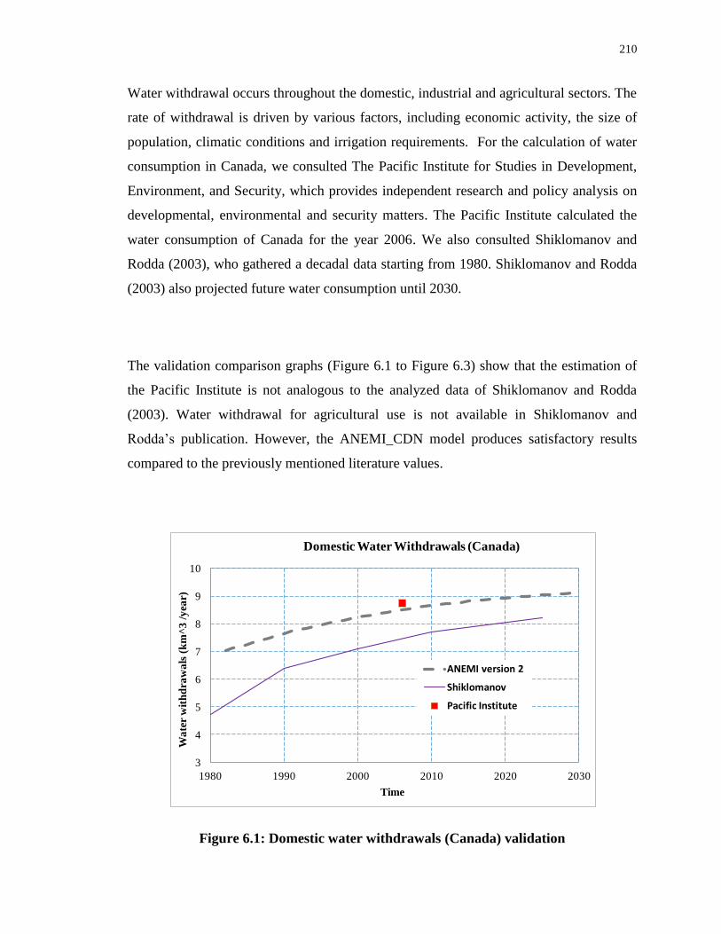
210

Water withdrawal occurs throughout the domestic, industrial and agricultural sectors. The

rate of withdrawal is driven by various factors, including economic activity, the size of

population, climatic conditions and irrigation requirements. For the calculation of water

consumption in Canada, we consulted The Pacific Institute for Studies in Development,

Environment, and Security, which provides independent research and policy analysis on

developmental, environmental and security matters. The Pacific Institute calculated the

water consumption of Canada for the year 2006. We also consulted Shiklomanov and

Rodda (2003), who gathered a decadal data starting from 1980. Shiklomanov and Rodda

(2003) also projected future water consumption until 2030.

The validation comparison graphs (Figure 6.1 to Figure 6.3) show that the estimation of

the Pacific Institute is not analogous to the analyzed data of Shiklomanov and Rodda

(2003). Water withdrawal for agricultural use is not available in Shiklomanov and

Rodda‘s publication. However, the ANEMI_CDN model produces satisfactory results

compared to the previously mentioned literature values.

Figure 6.1: Domestic water withdrawals (Canada) validation

3

4

5

6

7

8

9

10

1980 1990 2000 2010 2020 2030

Wa

ter

wit

hd

raw

als

(k

m^

3 /

yea

r)

Time

Domestic Water Withdrawals (Canada)

ANEMI version 2

Shiklomanov

Pacific Institute

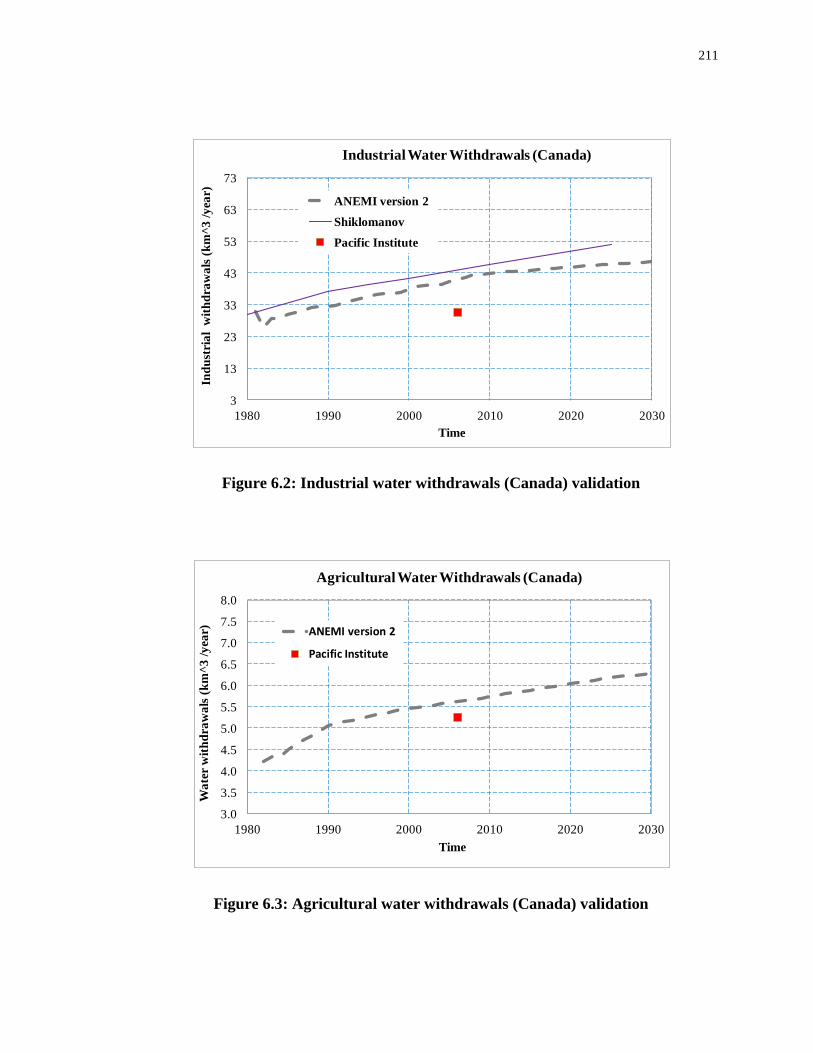
211

Figure 6.2: Industrial water withdrawals (Canada) validation

Figure 6.3: Agricultural water withdrawals (Canada) validation

3

13

23

33

43

53

63

73

1980 1990 2000 2010 2020 2030

Ind

ust

ria

l w

ith

dra

wa

ls (

km

^3

/y

ear)

Time

Industrial Water Withdrawals (Canada)

ANEMI version 2

Shiklomanov

Pacific Institute

3.0

3.5

4.0

4.5

5.0

5.5

6.0

6.5

7.0

7.5

8.0

1980 1990 2000 2010 2020 2030

Wa

ter

wit

hd

raw

als

(k

m^

3 /

yea

r)

Time

Agricultural Water Withdrawals (Canada)

ANEMI version 2

Pacific Institute

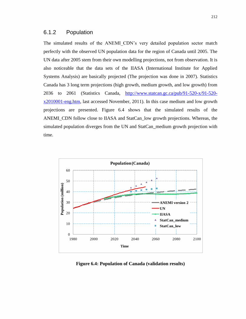
212

6.1.2 Population

The simulated results of the ANEMI_CDN‘s very detailed population sector match

perfectly with the observed UN population data for the region of Canada until 2005. The

UN data after 2005 stem from their own modelling projections, not from observation. It is

also noticeable that the data sets of the IIASA (International Institute for Applied

Systems Analysis) are basically projected (The projection was done in 2007). Statistics

Canada has 3 long term projections (high growth, medium growth, and low growth) from

2036 to 2061 (Statistics Canada, http://www.statcan.gc.ca/pub/91-520-x/91-520-

x2010001-eng.htm, last accessed November, 2011). In this case medium and low growth

projections are presented. Figure 6.4 shows that the simulated results of the

ANEMI_CDN follow close to IIASA and StatCan_low growth projections. Whereas, the

simulated population diverges from the UN and StatCan_medium growth projection with

time.

Figure 6.4: Population of Canada (validation results)

0

10

20

30

40

50

60

1980 2000 2020 2040 2060 2080 2100

Po

pu

lati

on

(m

illi

on

)

Time

Population (Canada)

ANEMI version 2

UN

IIASA

StatCan_medium

StatCan_low

213

6.1.3 Land-Use

Canada contains over one-third of the world‘s boreal forest, one-fifth of the world‘s

temperate rainforest, and one-tenth of the total global forest cover. These relatively

undisturbed forest areas are sufficiently large to maintain all of their native biodiversity.

However, they are increasingly being converted into either agricultural land or human

settlements. The land-use sector of the ANEMI_CDN model has the capability to

generate a land conversion rate based on the population growth. Two validation graphs

(Figure 6.5 and Figure 6.6) are presented to show future land-use change (i.e. conversion

of forest area to cultivated/agricultural area). The simulated results are also compared

with the WDI database (World Development Indicators, The World Bank,

http://databank.worldbank.org, last accessed, August 2011). The ANEMI_CDN

performance shows a good agreement with the observations. Unlike the observed data,

the ANEMI_CDN simulations show a rising trend in agricultural land use. Such a result

is expected by the majority of the scientific community.

Figure 6.5: Forest area (Canada) validation

250

260

270

280

290

300

310

320

330

340

350

1980 2000 2020 2040 2060 2080 2100

Are

a (

M. h

a)

Time

Forest Area (Canada)

ANEMI version 2

WDI Forest Area

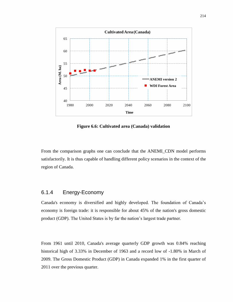
214

Figure 6.6: Cultivated area (Canada) validation

From the comparison graphs one can conclude that the ANEMI_CDN model performs

satisfactorily. It is thus capable of handling different policy scenarios in the context of the

region of Canada.

6.1.4 Energy-Economy

Canada's economy is diversified and highly developed. The foundation of Canada‘s

economy is foreign trade: it is responsible for about 45% of the nation's gross domestic

product (GDP). The United States is by far the nation‘s largest trade partner.

From 1961 until 2010, Canada's average quarterly GDP growth was 0.84% reaching

historical high of 3.33% in December of 1963 and a record low of -1.80% in March of

2009. The Gross Domestic Product (GDP) in Canada expanded 1% in the first quarter of

2011 over the previous quarter.

40

45

50

55

60

65

1980 2000 2020 2040 2060 2080 2100

Are

a (

M. h

a)

Time

Cultivated Area (Canada)

ANEMI version 2

WDI Forest Area

215

It seems difficult to find any reliable projections of GDP for Canada. Most projections

report a 1% change relative to baseline for policy experimentation. The simulated result

of ANEMI_CDN seems close to the WDI data from the World Bank

(http://databank.worldbank.org, last accessed, August 2011). (In this data, GDP is

expressed in constant 2005 international dollar value. However, the model does not have

money or inflation. All prices are in terms of real goods, so there is no need to adjust for

the value of a dollar across time.) The results thus satisfy the calibration of the energy-

economy sector of the Canada model (Figure 6.7).

Figure 6.7: Real GDP per capita for Canada

6.2 Regional ANEMI Model (ANEMI_CDN) Analyses

As stated previously, one of the main objectives of this study was to develop a regional

model for Canada that can help with the analysis of national climate change policies. In

0

5

10

15

20

25

30

35

40

45

50

1980 1985 1990 1995 2000 2005 2010 2015

Th

ou

san

d $

Time

GDP Per Capita (Canada)

ANEMI version 2

WDI_2005 int$

216

light of this objective, we used the ANEMI_CDN to analyze three selected policy

scenarios. The following sections present the results.

6.2.1 Canada Carbon Tax Scenario

In this section, we present some selected results of the regional model‘s analysis of the

first scenario—the implementation of a carbon tax in 2012. Each of the following figures

includes the baseline (no carbon tax applied) and the carbon-tax policy alternatives. The

carbon-tax policy simulations assume that Canada and the rest of the world (ROW)

implement the same policy: a carbon tax that begins in 2012 and slowly ramps up to $100

per tonne of CO2 over 30 subsequent years.

Figure 6.8 shows the GDP per capita for the baseline run and the carbon tax scenario. As

in the global model, the tax distortion initially reduces Canada‘s GDP. However, the

reduction in climate damages and the change in fossil fuel prices slowly take combined

effect and the GDP increases relative to the baseline. Granted, the benefit from the carbon

tax is somewhat offset in the regional model, since fossil fuel exports decrease under the

tax policy.

217

Figure 6.8: GDP per capita (Canada)

Figure 6.9 shows the total energy input that Canada would use in the production of

aggregate energy services. For the baseline (no tax implemented), the hump shape in the

total energy input is a result of increasing fossil fuel prices, which are given exogenously

from the global model. With the carbon tax, there is a significant impact on energy

consumption in the regional model. This effect is also visible in the simulations of the

global model.

0

10

20

30

40

50

60

70

80

1980 2000 2020 2040 2060 2080 2100

Tho

usa

nd

$

Time

GDP Per Capita (Canada)

With Tax

Base

218

Figure 6.9: Total energy used in the production of aggregate energy services

(Canada)

Figure 6.10 shows the total industrial emissions from the ANEMI_CDN model. These

emissions are closely linked with the total energy consumption. Similar to the global

model‘s simulation results, the carbon tax has a significant impact on fossil fuel

consumption and industrial emissions.

0

2

4

6

8

10

12

14

16

1980 2000 2020 2040 2060 2080 2100

10

9G

J

Time

Total Energy Used in the Production of Aggregate Energy

Services (Canada)

With Tax

Base

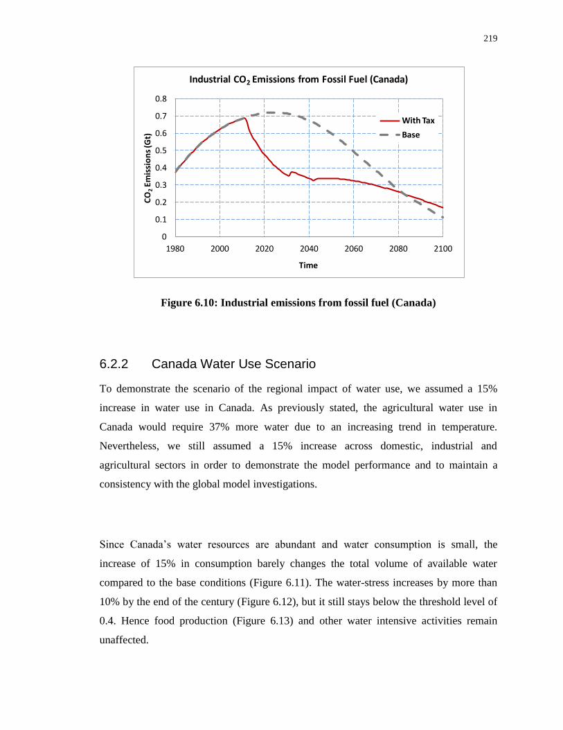
219

Figure 6.10: Industrial emissions from fossil fuel (Canada)

6.2.2 Canada Water Use Scenario

To demonstrate the scenario of the regional impact of water use, we assumed a 15%

increase in water use in Canada. As previously stated, the agricultural water use in

Canada would require 37% more water due to an increasing trend in temperature.

Nevertheless, we still assumed a 15% increase across domestic, industrial and

agricultural sectors in order to demonstrate the model performance and to maintain a

consistency with the global model investigations.

Since Canada‘s water resources are abundant and water consumption is small, the

increase of 15% in consumption barely changes the total volume of available water

compared to the base conditions (Figure 6.11). The water-stress increases by more than

10% by the end of the century (Figure 6.12), but it still stays below the threshold level of

0.4. Hence food production (Figure 6.13) and other water intensive activities remain

unaffected.

0

0.1

0.2

0.3

0.4

0.5

0.6

0.7

0.8

1980 2000 2020 2040 2060 2080 2100

CO

2Em

issi

on

s (G

t)

Time

Industrial CO2 Emissions from Fossil Fuel (Canada)

With Tax

Base

220

Figure 6.11: Available surface water (Canada)

Figure 6.12: Water-stress (Canada)

400

500

600

700

800

900

1000

1980 2000 2020 2040 2060 2080 2100

Su

rfa

ce w

ate

r (

km

^3)

Time

Available Surface Water (Canada)

Water use increase

Base

0.00

0.05

0.10

0.15

0.20

0.25

0.30

0.35

0.40

0.45

1980 2000 2020 2040 2060 2080 2100

Wa

ter

Str

ess(

dim

ensi

on

less

)

Time

Water Stress (Canada)

Water use increase

Base

221

Figure 6.13: Food production (Canada)

We know that increased water-stress seriously threatens human survival. Fortunately, for

the duration of the twenty-first century, the water-stress in Canada appears to remain

below the critical level. The region‘s large water resources and plentiful food stock thus

provide favorable conditions to sustain a very stable population up to the year 2100

(Figure 6.14).

Since the population of Canada remains almost unchanged (0.5% increase) with the 15%

increase in water consumption, the CO2 emissions from fossil fuel and GDP also remains

nearly unchanged (Figure 6.15 and Figure 6.16).

0

50

100

150

200

250

1980 2000 2020 2040 2060 2080 2100

Fo

od

(tri

llio

n k

ilo

calo

rie

/yr)

Time

Food Production (Canada)

Water use increase

Base

222

Figure 6.14: Population (Canada)

Figure 6.15: CO2 emissions from fossil fuel (Canada)

20

25

30

35

40

45

1980 2000 2020 2040 2060 2080 2100

Po

pu

lati

on

(M

illi

on

)

Time

Population (Canada)

Water use increase

Base

0

0.1

0.2

0.3

0.4

0.5

0.6

0.7

0.8

1980 2000 2020 2040 2060 2080 2100

CO

2em

issi

on

s (G

t)

Time

CO2 Emissions from Fossil Fuel (Canada)

Water use increase

Base

223

Figure 6.16: GDP (Canada)

6.2.3 Canada Food Production Increase Scenario

Over the past 40 years, the number of farms in Canada has declined. The remaining

farms, however, have become larger and more productive. A variety of factors has

contributed to this increase in food production: greater use of mechanization, mineral

fertilizers and pesticides, new and better crop varieties, and other innovative farming

practices. Granted, some of these advances have clearly compromised environmental

health, including water quality. The agricultural impact on water resources arise from the

need for additional water (semi-arid landscapes), the use of additional nutrients, the use

of pesticides, and so on.

It is expected that Canada would remain sufficiently capable of providing food for its

population the end of the twenty-first century. However, as a responsible member of the

global community, Canada may have to produce more food to meet the needs of the rest

of the world. In this scenario, the agricultural land conversion rate in Canada is increased

by 15% (the same rate as in global analyses). This regional increase allows for a

0

500

1000

1500

2000

2500

3000

3500

1980 2000 2020 2040 2060 2080 2100

GD

P (

bil

lio

n $

)

Time

GDP (Canada)

Water use increase

Base

224

demonstration of the model‘s utility, as well as a comparison with the results of the

global model.

In this scenario, the results of simulations are not the same at the regional and global

scales. For Canada, an increase of 15% in land conversion provides for a roughly 13%

increase in food production (Figure 6.17). At the global scale, however, the increase was

only around 1%. A 15% increase in agricultural land of course requires more water.

High water availability and low water demand in Canada still make the effect of

increased water consumption barely noticeable (Figure 6.18). Even though it increases

around 7% by the end of this century (Figure 6.19), water stress remains below the

critical threshold level.

Figure 6.17: Food production (Canada)

0

50

100

150

200

250

300

350

1980 2000 2020 2040 2060 2080 2100

Fo

od

(tri

llio

n k

ilo

calo

rie/

yr)

Time

Food Production(Canada)

Increase in food production

Base

225

Figure 6.18: Available surface water (Canada)

Figure 6.19: Water-stress (Canada)

Freshwater is essential for human survival, healthy ecosystems and sustainable

development. Fortunately, Canada has plenty of freshwater resources to support its

population. And yet surprisingly the regional model results do not show any visible

400

500

600

700

800

900

1000

1980 2000 2020 2040 2060 2080 2100

Su

rfa

ce w

ate

r (k

m^

3)

Time

Available Surface Water (Canada)

Increase in food production

Base

0.00

0.05

0.10

0.15

0.20

0.25

0.30

0.35

0.40

0.45

1980 2000 2020 2040 2060 2080 2100

Wa

ter

Str

ess(

dim

ensi

on

less

)

Time

Water Stress (Canada)

Increase in food production

Base

226

population growth (Figure 6.20). (The global population, on the other hand, slightly

increases by the end of this century.) This tiny increase in population growth in the region

of Canada can be explained by sufficient food production and/or the optimum availability

of per capita food-energy. A further increase in per capita food production does not

change the life expectancy in Canada.

Figure 6.20: Population (Canada)

The total population in Canada remains almost unchanged, even with the 13% increase in

food production. With negligible change in population, there is also no increase in human

induced fossil fuel based emissions, and no visible increase in GDP. Both the GDP and

fossil fuel based emissions thus remain almost unchanged (Figure 6.21 and Figure 6.22).

20

25

30

35

40

45

1980 2000 2020 2040 2060 2080 2100

Po

pu

lati

on

(M

illi

on

)

Time

Population (Canada)

Increase in food production

Base

227

Figure 6.21: CO2 emissions from fossil fuel (Canada)

Figure 6.22: GDP (Canada)

0

0.1

0.2

0.3

0.4

0.5

0.6

0.7

0.8

1980 2000 2020 2040 2060 2080 2100

CO

2em

issi

on

s (G

t)

Time

CO2 Emissions from Fossil Fuel (Canada)

Increase in food production

Base

0

500

1000

1500

2000

2500

3000

3500

1980 2000 2020 2040 2060 2080 2100

GD

P (

bil

lio

n $

)

Time

GDP (Canada)

Increase in food production

Base

228

6.3 Summary

In this chapter, we compared the results of the ANEMI_CDN model simulations with the

available historical observations and literature values. The comparisons show that the

ANEMI_CDN performs satisfactorily as a feedback based society-biosphere-climate-

economy-energy system model for Canada. Such a performance proves that the

regionalized ANEMI model (ANEMI_CDN) can be used for the analyses of future

climate change scenarios.

We simulated three different climate change policy scenarios using the ANEMI_CDN

model. These scenarios were either related to emerging problems (shortage in food

production, shortage in water availability, etc.) or to preventive climate change mitigation

measures such as emissions reductions. They allowed us to test the model‘s capacity to

deal with the behaviours of a complex system. For each of these scenarios, we selected

arbitrary quantitative values to test the model performance. The scenarios we investigated

were the following:

o Implementation of carbon tax as well as carbon capture and storage technology

o 15% increase in overall water use; and

o 15% increase in agricultural land conversion.

The simulations of the same scenarios do not show the same results on global and local

scales. We may attribute this to the spatial distribution of resources and climate impacts.

The increased water use scenario revealed an alarming rise in global water-stress levels,

coupled with a sharp reduction in food production. Such unfavorable results would

threaten current population growth, and would indeed lead to a small decrease in the

future population. In Canada, however, the population would not decrease. Even with the

extra pressure on Canada‘s water resources, the water-stress level would remain far

229

below the critical threshold. The related changes in GDP, atmospheric CO2

concentration, and atmospheric temperature would likewise be insignificant.

In the land increase scenario, the 15% conversion rate to agricultural land leads to a mere

1% increase in food production at the global scale. A closer investigation reveals that the

extra agricultural activities would (a) add more pressure on the already scarce water

resources and (b) would increase the fresh water demand for dilution. Given the feedback

structure of the model, water scarcity thus restricts food productivity. In Canada, on the

other hand, the added agricultural land leads to a 13% increase in food production. This

contrasting value is due to a much lower level of water-stress in Canada. Other related

model sectors also show only minor changes. The only visible change is in atmospheric

CO2 concentration, which is a result of the clearing and burning of forests required for the

development of new agricultural land.

In the case of the carbon tax scenario, the carbon capture and storage technology is

introduced. After implementing a moderate tax policy, the model shows a significant

reduction in CO2 emissions from fossil fuel and a stabilization of the atmospheric CO2

concentration. Carbon capture and storage technology can thus be implemented to lower

the atmospheric CO2 concentration below 500 ppm level. These combined efforts lower

the global temperature and the sea-level rise when compared to current policy

environment. The carbon tax implementation does not significantly affect any of the

other sectors of the model.

Taken together, these analyses amply demonstrate the robustness of the model and its

readiness to be applied in the investigation of various climate change mitigation and

adaptation policy options.

230

CHAPTER 7

7 OPTIMIZATION AND SIMULATION FOR THE INTEGRATED ASSESSMENT MODELLING

The ANEMI model version 1.2 is a system dynamics simulation model that integrates

nine sectors, including an economic sector. However, the economic variables in that

version of the model are formulated in an overly simplified fashion. Indeed the price and

demand calculation procedures are not capable of fulfilling the classical macroeconomic

principle of the fundamental equilibrium between supply and demand. Hence the

investment funds allocated to generate electric energy are endogenous (prescribed).

Davies and Simonovic (2009) characterized the economic sector of the ANEMI model

version 1.2 as myopic, since the decisions are based on historical behaviour.

Supply and Demand model is the most important model in free market economics. It

asserts that free markets can allocate resources without instructions from a central

authority. In macroeconomics, the most common way to solve the problems of supply

and demand is computationally, by employing various iterative algorithms. In order to

develop a concrete energy-economy sector for the ANEMI model, it is thus necessary to

incorporate a market clearing mechanism to attain the fundamental equilibrium between

supply and demand. The ANEMI model version 2 involves energy-economic agents

maximizing their objective function under various constraints. This increases the

complexity and sophistication of the model.

The optimization capability of the Vensim software is very limited. The discrete nature of

the energy-economy sector constitutes an added complexity with respect to software

integration and program computational time. Consequently, in each simulation time step

the model must call in an outside optimization program for the solution of important

231

variables within the energy-economy sector. Such a complex mathematical formulation

and multifaceted mechanism demands this, separate, Chapter on optimization and

simulation for the integrated assessment modelling.

7.1 Optimization Simulation Model

A simulation model can be defined as a mathematical model or representation of a

physical, biological or informational system or process. Simulation models include key

inputs that affect the model as well as corresponding outputs. Simulation models are

supposed to accurately predict a system‘s response to a given design configuration and

provide an in-depth analysis of that response. The simulation predicts the outcome of a

single, specified set of design or policy variables.

Of course, the space of suitable design and policy variable values is practically infinite.

As important tools for managing systems, simulation models do not identify or narrow

the search area for design and policy alternatives; they provide only localized information

regarding the response of the system to one particular design alternative at a time. Still,

optimization models can screen the alternatives and thus reduce the number that need to

be simulated in detail. They search the space of possible design variable values and

identify an optimal design and/or operating policy for a given system design objective

and set of constraints. Optimization models are thus generally used for the preliminary

evaluation or screening of alternatives. They thus identify important data needs prior to

extensive data collection and simulation modelling activities (McKinney and Savitsky,

2003). The objective of any optimization process is to coordinate the simulation of a

sequence of system configurations, where each configuration corresponds to particular

settings of the decision variables. Therefore, a system configuration is ultimately

obtained that provides an optimal or near optimal solution (Law and McComas, 2000).

232

As stated above, the ANEMI model version 1.2 represented economic variables and

decisions in an overly simplified way. In it, investment funds for electricity generation

are prescribed and then allocated; therefore, the total investment is dynamic only in the

sense that it meets the demand, which rises over time through economic development.

Because of its simulation based structure, the energy demand is also represented in a

simple fashion that does not adequately capture historical changes in behaviour.

Moreover, the economic output is not tied to energy demand or prices, and this leads to

the dramatic rise and fall of energy prices without affecting the economic system.

In light of these shortcomings, this research has striven to develop an improved energy-

economy sector for the ANEMI model (ANEMI version 2 and ANEMI_CDN), in which

the missing links between the energy and economy subsectors can be restored and the

fundamental equilibrium between supply and demand can be satisfied. The most useful

method to satisfy such criteria involves the use of various iterative methods, where

optimization is overwhelmingly utilized throughout the macroecomic field. Hence in this

newer version of the system dynamics simulation model ANEMI (ANEMI version 2 and

ANEMI_CDN), optimization is integrated in the energy-economy sector and

optimization techniques are used to search the space of possible variable values and to

identify an optimal design and/or operating policy.

7.1.1 Optimization Problem Definition

The main elements of any constrained optimization problem are:

• Decision variables - are unknown at the beginning of the optimization process and the

goal is to find the best values that can produce the most desired objective function. A

decision variable can be instantiated only in the context of a given model instance.

233

• Objective function - is a mathematical expression that combines the variables to express

the goal. It indicates how much each variable contributes to the value to be optimized in

the problem. The objective function takes the following general form:

,

Subject to:

where is the objective function coefficient corresponding to the jth

variable, and is

the jth

decision variable, represents the technological coefficient, is the right-hand

side coefficient, is the total number of constraints, and is the total number of

decision variables. The coefficients of the objective function indicate the contribution to

the value of the objective function of one unit of the corresponding variable. For

example, if the objective function is to maximize the present value of a project, and is

the jth

possible activity in the project, then (the objective function coefficient

corresponding to ) gives the net present value generated by one unit of activity . As

another example, if the problem is to minimize the cost of achieving some goal, might

be the amount of resource j used in achieving the goal. In this case, would be the cost

of using one unit of resource .

• Constraints - are conditions that a solution to any optimization problem must satisfy.

These are mathematical expressions that combine the variables to express limits on the

234

possible solutions. There are two types of constraints: equality constraints and inequality

constraints.

• Variable bounds – are the extreme points after which the solutions are not acceptable in

the optimization process. For example, zero and 100 might bound the production

capacity of a particular machine.

7.1.2 Model Structure and Application

Until the end of the last millennium, optimization and simulation were kept largely

separate in practice. Kasperska et al. (2000; 2001) embedded optimization procedures in

their system dynamics simulation models, while optimizing the dynamics balance of a

production process. They dealt with two methods of embedding optimization procedures

in the simulations of models type SD. The first way they undertook the problem was in

relation to Legras’s idea regarding the so-called "pseudosolution" of equation:

, which minimizes the norm of these differences. Here, is a vector of a known

coefficient, represents the vector of variables, and is a (known) matrix coefficient. In

the second way that they approached the problem, they took advantage of the Linear

Programming optimization. They called this approach "embedding linear programming

in System Dynamics" (Kasperska et al., 2003).

Taking into account the non-linear nature of the energy-economy sector, the ANEMI

model version 2 and ANEMI_CDN choose a nonlinear system of equations as an

optimization tool, which utilizes the trust-region method (with dogleg algorithm). As

these models have a significant number of nonlinear equations to solve, the Gauss-

Newton method with a line search is not a robust choice.

235

It is clear from a review of the available literature that simulation based optimization has

been used primarily in computer and chemical engineering for supply chain management

(Truong and Azadivar, 2003; Hung et al., 2004; Erdem and Sancarin, 2006; Almeder and

Margaretha, 2007; Amodeno et al., 2009). However, side by side simulation based

optimization techniques have also attracted water resources management researchers

(Bhattacharjya and Datta, 2005; Fedra and Harmancioglu, 2005; Pulido-Velazquez et al.,

2006; Cetinkaya et al., 2008; Safavi et al., 2009; Bashi-Azghadi et al., 2010; Singh,

2011). Apart from these, such approaches have also been well accepted in other

computational arenas, such as risk management (Better et al., 2008) and fishery

management (Azadivar et al., 2002).

For the last ten years, only a few optimization based simulation models have been

available in the field of integrated assessment modelling. These include MERGE (Manne

et al., 1995), REMIND (Luderer et al., 2009; Leimbach et al., 2010), and MiniCAM

(Calvin et al., 2009). MERGE solves in each period the optimal emissions prices that

meet a long-term target. So at each point in time, supply and demand are equilibrated

through the price of the internationally traded commodities: oil, gas, coal, carbon

emissions rights and a numeraire good (composite of all items produced outside the

energy sector). REMIND is a global energy-economy-climate model that uses inter-

temporal optimization. It is actually an optimal growth model in which inter-temporal

global welfare is optimized according to equilibrium constraints. MiniCAM is a

recursive partial equilibrium model with a long-term time horizon that runs in 15-year

time steps. In the MiniCAM model, the focus is on energy and agriculture, i.e. the

clearing of energy and agricultural goods.

The ANEMI version 2 and ANEMI_CDN differ from the above mentioned IAMs. Their

uniqueness stems from the way they merge a system dynamics approach with a neo-

classical growth model in which feedbacks keep the model in a very dynamic state. Other

models can only focus on long term problems for which they have known resource paths.

236

Optimization is carried out to distribute the investment optimally over time. Because of

its unique system dynamics based feedback structure, however, our new version of the

ANEMI model is solving 1 time problem (such that optimization is carried out based on

the current state). MERGE has more detailed energy sector compared to the available

IAMs, except for the ANEMI model (ANEMI version 2, ANEMI_CDN). MERGE takes

into account different fossil fuel energy sources while computing the energy price. But in

calculating the energy price, new version of the ANEMI takes into account not only

known fossil fuel energy reserves; it also takes into account probable energy discoveries

(for each type of fossil fuel), availability of hydro and nuclear energy, and technological

changes.

Optimization Simulation Structure

Optimization and simulation are carried out side by side in the energy-economy sector

(Figure 7.1). The price of fuel and the capital stocks for energy production are simulated

based on the optimal value of GDP, energy production and energy use across different

sectors. In the ANEMI model (ANEMI version 2 and ANEMI_CDN), the optimal value

of these components are driven by the optimization scheme in relation to the population

and climate sectors as well as the energy sector. The optimization scheme of this ANEMI

model also requires two more variables from sectors outside of the energy-economy

complex: labour and climate damage function. The population sector supplies labour

force to the model, which is comprised of the total population between the ages of 15 and

64. The damage function here stands for the economic damage due to sea-level rise,

flood, drought and so on; it is the consequence of global temperature change. The global

temperature is mostly influenced by radiative forcing: it is simulated within the climate

sector of the ANEMI model.

237

Figure 7.1: Basic computational flow chart of the energy-economy sector of the

ANEMI model (ANEMI version 2 and ANEMI_CDN)

7.1.3 Mathematical Formulation of the Optimization-Simulation Problem in ANEMI Version 2

In the current version of the ANEMI model (ANEMI version 2 and ANEMI_CDN), we

define such optimization criteria as the consumption of good and average total cost of

energy as objective functions comprising numerical measures that are used to compare

the model output (for example, fossil fuel consumption) with user specified targets at

each time step of the simulation. Based on the calculated objective functions, the

optimization algorithm selects new sets of control parameters to be evaluated. The

process is repeated for a number of times until no further improvement can be made. The

governing nonlinear system of equations under the optimization scheme is presented by

Equations 7.1 to 7.15. Equations 7.16 to 7.23 under the simulation environment are

mainly responsible for producing input data for the optimization scheme. The stated

238

equation numbers in Figure 7.2 represent the relevant equations that connect optimization

and simulation in the latest version of the ANEMI model.

Figure 7.2: Schematic view of simulation based optimization scheme

The world‘s population is assumed to be represented by a stand-in household whose

preferences can be represented by the utility function

where is a generic consumption good. The household supplies labour, , inelastically to

the market. We assume that the household owns the world‘s capital stock and natural

resources. Thus, the consumer rents the capital to the firm, so

where is the interest rate and is the aggregate capital stock in the economy. The

consumer also sells energy services to the firm, so

Real World Simulation Model

Computer Implementation (Optimization)

GDP,energy consumption

labour force, temperature,

energy reserve, capital

7.25, 7.28

7.267.34, 7.35

7.25, 7.28

7.27

7.30, 7.31

Equation number

239

where is aggregate energy services, and is the price of aggregate energy services.

The consumer also sells labour services to the firm, thus

where is the wage rate and is the labour force. Investment, , is assumed to follow a

Sollow investment rule where a fraction of output, , is invested into new capital each

period. Total investment is also equal to the sum of investment into aggregate capital ( )

and investment into electricity producing capital for coal, oil, natural gas, hydro power

and nuclear energy, which are denoted as ,

, ,

, and

and

Consumption is equal to the total output minus total investment

240

Total tax from the carbon emissions by fossil fuel consumption, , is the sum of tax

revenues from carbon emissions by fossil fuel consumption

where is the fuel specific emissions tax and is fossil fuel consumption for each

specific type.

Given prices, the objective of the household is to maximize utility subject to its budget

constraint. Each period the household‘s problem is:

Objective function of the household:

or

Budget constraints of the household:

or

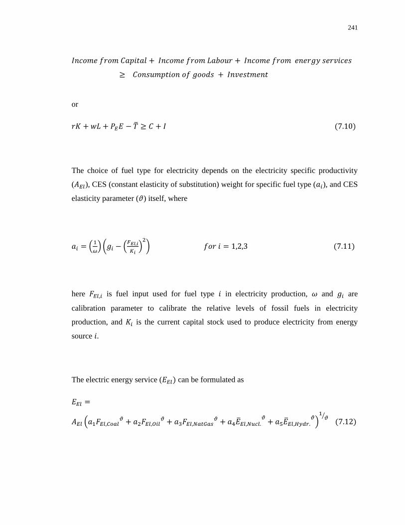
241

or

The choice of fuel type for electricity depends on the electricity specific productivity

( ), CES (constant elasticity of substitution) weight for specific fuel type ( ), and CES

elasticity parameter ( ) itself, where

here is fuel input used for fuel type in electricity production, and are

calibration parameter to calibrate the relative levels of fossil fuels in electricity

production, and is the current capital stock used to produce electricity from energy

source .

The electric energy service ( can be formulated as

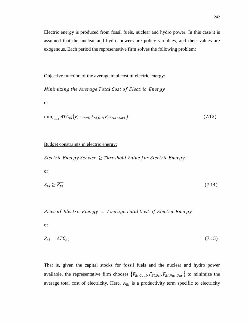
242

Electric energy is produced from fossil fuels, nuclear and hydro power. In this case it is

assumed that the nuclear and hydro powers are policy variables, and their values are

exogenous. Each period the representative firm solves the following problem:

Objective function of the average total cost of electric energy:

or

Budget constraints in electric energy:

or

or

That is, given the capital stocks for fossil fuels and the nuclear and hydro power

available, the representative firm chooses to minimize the

average total cost of electricity. Here, is a productivity term specific to electricity

243

production, is the fuel input used for fuel type in electricity production, and is the

CES elasticity parameter, where elasticity of substitution of

The functions , for the fossil fuels, are decreasing in the fuel-to-capital ratio. Inside a

period this assumption implies diminishing returns, as capital is a fixed factor. The

parameters and are fixed. The parameters and are used to calibrate the relative

levels of fossil fuels in electricity production.

The choice of fuel type for heat energy depends on the heat energy specific productivity

( ), CES weight for fuel type ( ), and CES elasticity parameter ( ) itself for heat

energy, where

There is no capital in the heat energy sector. The capital for heat energy comprises part of

the aggregate capital for the economy. The firm chooses

to minimize the average total cost of heat energy.

The structure for the production of heat energy is symmetric to the production of electric

energy. It is assumed that heat energy is produced from fossil fuels and alternative energy

sources. Each period the representative firm solves the following problem:

244

Objective function for average total cost of heat energy:

or

Budget constraints for heat energy:

Or

Or

The world‘s production of final output is represented by a stand-in firm which employs a

Cobb-Douglas production technology. The firm hires labour, capital, and energy services

from the stand-in household and produces the generic consumption of goods.

The aggregate production function is:

245

where,

here, is total factor productivity (TFP), are parameters for damage function,

and is the Nordhaus damage coefficient. The damage coefficient is a function of ,

global mean temperature.

The available supply of investments funds for electricity production is assumed to follow

a Solow rule. That is, each period is available to invest in new electricity capital:

here is the current capital stock used to produce electricity from energy source ,

which could be either a fossil fuel, nuclear or hydro power. without a subscript is the

aggregate capital stock for the economy, Investment, is the fraction of the output, , is

invested into new capital in each period.

For the one period problem the capital and labour inputs are fixed. Demand for aggregate

energy services can be expressed as:

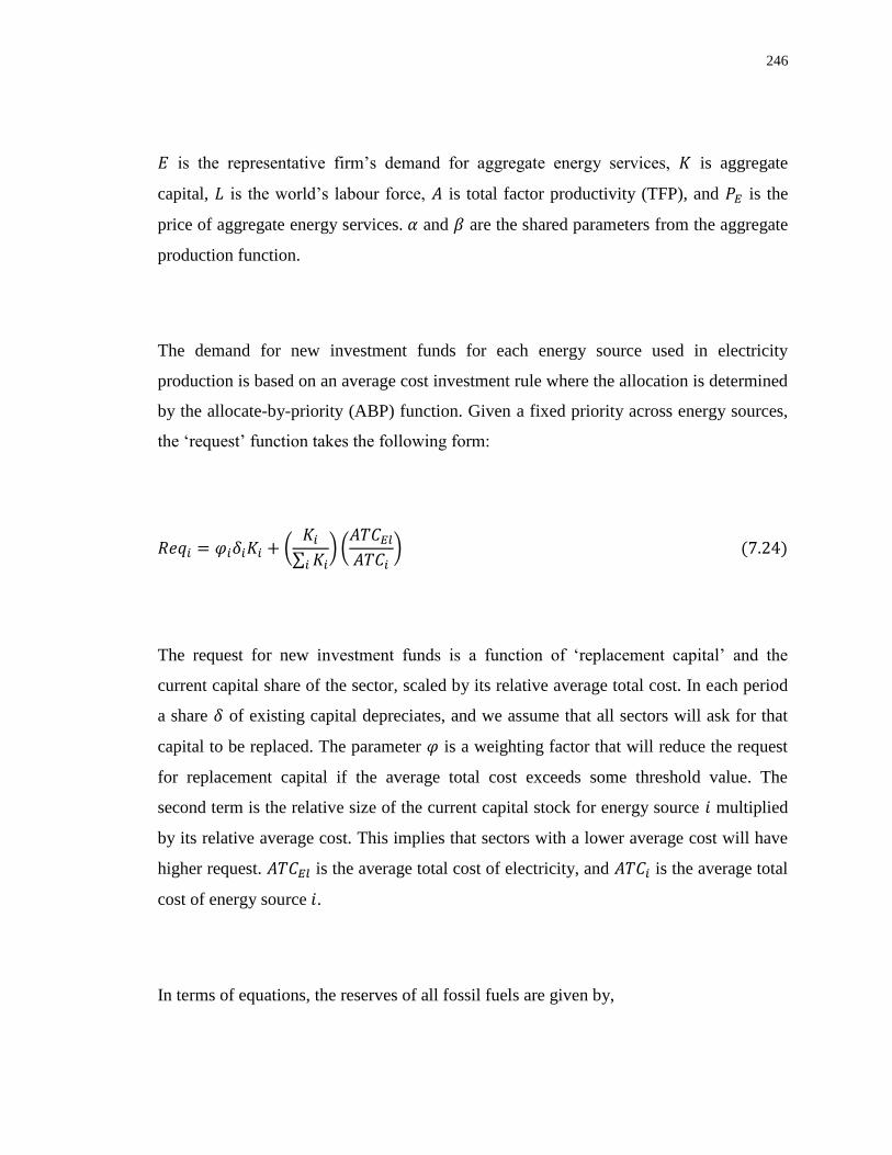
246

is the representative firm‘s demand for aggregate energy services, is aggregate

capital, is the world‘s labour force, is total factor productivity (TFP), and is the

price of aggregate energy services. and are the shared parameters from the aggregate

production function.

The demand for new investment funds for each energy source used in electricity

production is based on an average cost investment rule where the allocation is determined

by the allocate-by-priority (ABP) function. Given a fixed priority across energy sources,

the ‗request‘ function takes the following form:

The request for new investment funds is a function of ‗replacement capital‘ and the

current capital share of the sector, scaled by its relative average total cost. In each period

a share of existing capital depreciates, and we assume that all sectors will ask for that

capital to be replaced. The parameter is a weighting factor that will reduce the request

for replacement capital if the average total cost exceeds some threshold value. The

second term is the relative size of the current capital stock for energy source multiplied

by its relative average cost. This implies that sectors with a lower average cost will have

higher request. is the average total cost of electricity, and is the average total

cost of energy source .

In terms of equations, the reserves of all fossil fuels are given by,

247

where is the current energy source reserve, with initial values given in section (See

Table 3.4). is the resource discovery rate, and

is the calculated resource

depletion rate.

The total extraction of energy from any fossil fuel source or depletion has this form,

where is energy resource extraction for electricity production, and is non-electric

(heat) resource extraction.

Capital is the accumulation of the difference between investment and depreciation over

time, which can be written as

where is the total capital, is the investment, and is depreciation.

Capital for electric energy production ( ) has the same format as Equation (7.27), except

it considers investment and depreciation for electric energy

248

where and

are the investment and depreciation for electricity production in

respect to the source of fossil fuel type .

In this model, the price of fossil fuel mainly depends on the future fossil fuel reserve.

However, the elasticity parameter for fossil fuel price function ( ), base year price of

fossil fuel ( ), and their reserve, are all influencing the current fossil fuel price ( )

as well.

where is the base year reserve for each type of fuel. Equation 7.29, can be further

modified to take care of the carbon tax ( ) policy and can be rewritten as

7.2 Limitations

While optimization is supposed to have a considerable future in the simulation field, it

still suffers from the following limitations:

249

The optimization problem is complex. As optimization consists of nonlinear objective

functions, linear and nonlinear equalities and inequalities, it becomes difficult to define

the search region. Hence optimization requires a long computational time. Moreover, we

are also considering the implementation of the optimization techniques on some other

sectors of the ANEMI model. But this will add more complexity to the computational

scheme, and the chance of model break down will increase.

The energy-economy sector of the model is sensitive to changes in certain key parameters

because of the optimization approach in the modelling of electric energy production. The

problem occurs when a fossil fuel type starts to run low and its price becomes high

relative to the other fuel sources. As the capital stock does not adjust optimally, the

average total cost of electricity production for the fossil fuel type increases exponentially,

causing the model to break down. The problem is exacerbated by the functional form

chosen for the CES weights in the production function for electricity.

There are many ways of integrating optimizing processes within a simulation model. But

many of them have not been integrated, not only because they often require a

considerable amount of technical sophistication on the part of the user, but also because

of the aforementioned longer computational time.

250

CHAPTER 8

8 DISAGGREGATION FOR REGIONALIZATION OF ANEMI MODEL

Despite its improvements, the ANEMI model version 2 requires further enhancement in

one particular area. Its individual sectors represent socio- economic and natural processes

at a global scale, and therefore omit important regional processes. Therefore, we have

introduced a regional model (the ANEMI_CDN) that can test climate-change adaptation

and mitigation strategies for different regions of the world. For such strategies, of course,

the representation of regional effects is critical. A focus on regionalization allows the

modeler to investigate the differential effects of global climate change on regional water

resources, economic performance, energy supply and demand, land use, and energy.

Regional strategies can thus be based on more localized geographic and economic

factors.

As stated previously, the climate, the carbon cycle and a part of hydrological cycle will

remain at a global scale. In order to be combined together, these two different spatial

resolutions (global and regional) require some kind of mechanism to keep the feedback

loop active. Hence we introduced disaggregation modelling, which has the attractive

feature of being able to preserve most of the statistical properties while disaggregating

the global data into the regional one.

Disaggregation modelling has recently become one of the main techniques of hydrologic

time series modelling. Modelling rainfall and flow series at useful temporal and spatial

scales for various applications has been a difficult problem for a long time. Since the

1960s, researchers have been trying to resolve this issue, so that appropriate temporal and

251

spatial scales can be maintained without sacrificing the statistical characteristics (standard

deviation, skewness coefficient and lag-one correlation coefficient).

The first disaggregation approach was introduced by Harms and Campbell (1967). At that

stage, it was far less complex and sophisticated than it has come to be. At the initial stage

of disaggregation modelling, only a few models were developed. These included the H-C

model (Harms and Campbell, 1967), and the Box- Jenkins model (Box and Jenkins,

1970) but such models failed to fulfill the current simulation requirement.

Valencia and Schaake (1973) developed the first well-accepted disaggregation model by

developing the Valencia-Schaake technique (VLSH). Later, Mejia and Rouselle (1976)

modified the technique and developed another model, known as the Mejia and Rouselle

(MJRS) model. The periodic autoregressive (PRP) model (Salas et al., 1980) and the

periodic autoregressive and moving average (PARMA) model (Vecchia, 1985) have

proved viable options to model the seasonally varying correlation structure and to

preserve the stationary statistical properties within each season. In many cases, rainfall is

disaggregated/regionalized and applied in different contexts: such cases include Onof and

Wheater (1993), Onof et al. (1996), Wheater et al. (1999; 2005), Cowpertwait (1994),

Khaliq and Cunnane (1996), Verhoest et al. (1997), Gyasi-Agyei and Willgoose (1997),

Foufoula-Georgiou (1998), and Cowpertwait et al. (2002). Salas et al. (1980) mentioned

that this type of disaggregation is mostly applied in the temporal scale, but Lane (1979)

applied the same principal in the spatial domain. Burn (1997) introduced seasonality

measures as catchment similarity indices for regional flood frequency analysis (Pinault

and Allier, 2007).

The integration of the disaggregation model with the regional model ANEMI_CDN

proved quite difficult. However, in comparison to conventional autoregressive modelling,

the disaggregation model‘s added benefits made the required effort worthwhile. These

252

benefits include increased flexibility and a reduced number of parameters. Of course, in

dealing with such climate change related matters as weekly or monthly temperatures and

precipitation, the ANEMI_CDN faces not only the matter of spatial resolution, but also

the issue of the temporal scale.

8.1 Disaggregation Modelling

Salas et al. (1980) define disaggregation modelling as a process by which further time

series are generated from a time series already available. In the process of disaggregation

the original series is defined as the key series. A linear model is used to generate the

subseries from the key series. Such an approach helps to preserve the statistical properties

at both key and subseries levels, and to ensure the relationship between these two levels.

Disaggregation modelling can take two basic forms: temporal and spatial. An example of

the temporal kind would be the disaggregation of monthly rainfall from yearly rainfall.

Suitable examples of the spatial kind would include finding the tributary flow from a

natural flow of a river basin, and generating regional data from global data sets.

The attraction of disaggregation modelling is that it is not limited to only one level. This

method is initially capable of disaggregating yearly data into semi-annual time series, and

subsequently disaggregating the semi-annual time series into monthly values. The

disaggregation could continue further from monthly to weekly, maintaining the statistical

properties at a tolerable range.

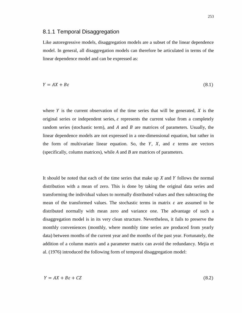
253

8.1.1 Temporal Disaggregation

Like autoregressive models, disaggregation models are a subset of the linear dependence

model. In general, all disaggregation models can therefore be articulated in terms of the

linear dependence model and can be expressed as:

where is the current observation of the time series that will be generated, is the

original series or independent series, represents the current value from a completely

random series (stochastic term), and and are matrices of parameters. Usually, the

linear dependence models are not expressed in a one-dimensional equation, but rather in

the form of multivariate linear equation. So, the , , and terms are vectors

(specifically, column matrices), while A and B are matrices of parameters.

It should be noted that each of the time series that make up and follows the normal

distribution with a mean of zero. This is done by taking the original data series and

transforming the individual values to normally distributed values and then subtracting the

mean of the transformed values. The stochastic terms in matrix are assumed to be

distributed normally with mean zero and variance one. The advantage of such a

disaggregation model is in its very clean structure. Nevertheless, it fails to preserve the

monthly conveniences (monthly, where monthly time series are produced from yearly

data) between months of the current year and the months of the past year. Fortunately, the

addition of a column matrix and a parameter matrix can avoid the redundancy. Mejia et

al. (1976) introduced the following form of temporal disaggregation model:

254

where is a parameter matrix with the same dimensions as , is a column matrix

containing monthly values from the previous year.

From the above equation, Lane (1979) developed a condensed form of the disaggregation

model, where the numbers of parameters are reduced by attributing zero value to the

unimportant parameters. The condensed model can be expressed as:

where and respectively denote the current time and immediate previous year.

Now, in a situation of disaggregating yearly rainfall, inputs are allocated into monthly

values: would have dimensions of 12 by 1 (12 monthly values), would have

dimensions of 1 by 1 (1 annual value for 1 station), would have dimensions of 12 by 1,

and the parameter matrices and B would have dimensions of 12 by 1 and 12 by 12,

respectively. Parameter is responsible to keep the linkage between the current month

and the previous month of the previous year (as for example in case of calculating the

rainfall of December 1980, will represent the rainfall of the November, 1979). So,

parameters and would have dimensions of 12 by 11 and 11 by 1, respectively.

It may be worthwhile to mention at this stage that time series modelling is not meant to

produce an exact result; rather, its aim is to produce an estimated value that should be

very close to a real one. The estimated model will therefore appear as following, where

the estimated value of , , , and are represented as , respectively.

255

Parameter Estimation

For this model, the following notations are used: the periodic (monthly) data are denoted

as ; ; and ; with being the year, and being the interval

(month) of the year. The limits and are represent respectively the total number of

years of data and the total number of intervals in the year.

The basic model has precisely the form of the linear dependence model. The parameter

estimates are exactly the same as the linear dependence model. is the matrix of

covariances among the monthly series; is the matrix of covariances between the

monthly and annual series; is the matrix of covariances among annual series, and so

on.

The estimates of the parameter matrices , and of the model equation are given from

(8.5)

and

Or equivalently

256

Note that the parameter estimate for is not given, but rather an estimate for is

stated in Equations 8.7 and 8.8. The following solution techniques will help in having an

estimate for B from

It requires the solution of the matrix equation . That is, given that the element of

the matrix D is known, it is necessary to find the element matrix B such that the product

of B times its transpose is equal to . To resolve this issue, the Choleskey

decomposition algorithm is used, which will be described later.

The estimation of parameter matrices , and as given Equations 8.5, 8.7 and 8.6

respectively require the sample covariance matrices , , , , ,and .

Where they can be expressed as:

(8.9)

(8.10)

Or

(8.11)

257

(8.12)

Or

(8.13)

Or

(8.14)

(8.15)

Or

(8.16)

Or

(8.17)

(8.18)

258

Or

(8.19)

(8.20)

Or

(8.21)

Or

(8.22)

The Choleski Decomposition

In linear algebra, the Cholesky decomposition or Cholesky triangle is a decomposition of

a Hermitian, positive-definite matrix into the product of a lower triangular matrix and its

conjugate transpose. André-Louis Cholesky formulated this method for real matrices (an

example of a square root of a matrix).

When the matrix is symmetric and positive definite, it is possible to perform the

symmetric decomposition

259

(8.23)

where

(8.24)

is a lower-triangular matrix. In fact, it is also possible to perform a Gauss elimination in a

symmetric fashion for symmetric positive definite matrices without pivoting for stability.

The Choleski algorithm (Wilkinson, 1965) is derived directly from Equation 8.23 as

(8.25)

Note that the summation runs only from 1 to the minimum of i to j due to the triangular

nature of . Thus

(8.26)

So that

(8.27)

Furthermore

(8.28)

So that we obtain

(8.29)

Considering the column of which is defined for by

260

(8.30)

With the diagonal element determined first by setting . It is clear that every element

in the right-hand side of Equation 8.30 comes from column ,....., ( ) of or from

column of .

Box-Cox transformation

In statistics, it is often necessary to transform the data to make the distribution close to

standard normal distribution for stabilizing variance. This improves the correlation

between variables. In this connection the Box–Cox transformation method was developed

by the statisticians George E. P. Box and David Cox in 1964 (Box and Cox, 1964). It is

one of the most useful data (pre)processing techniques.

Box-Cox transformation method finds the maximum likelihood estimates of the

parameters of the Box-Cox transform, the coefficients of the independent variables, and

the standard deviation of the normally distributed errors for a model in which a dependent

variable is regressed on independent variables. Any variable to be transformed must be

strictly positive. Depending on the requirement, the transformations can be classified as:

transformation of the dependent variables, which affects the relationship of the

dependent variable with all of the predictor variables in the model;

transformation of the individual predictor variables; and

transformation of both dependent and independent variables.

261

However, transformation may not be able to rectify all of the problems in the original

data; the regression analysis may still be suspect.

The parameter , possibly a vector, defining a particular transformation can be used for

the transformation of to .

(8.31)

The transformation (Equation 8.31) holds for Y> 0. Since an analysis of variance is

unchanged by a linear transformation (Equation 8.31) is equivalent to

(8.32)

the form (Equation 8.31) is slightly preferable for the theoretical analysis because it is

continuous at λ=0. In general, it is assumed that for each λ, is a monotonic function

of over the admissible range.

Steps in practical application

While formulating the basic disaggregation equations (Equations 8.3 and 8.33), it is

assumed that and are normally distributed. It is found that in the GCMs, the analyzed

data sets of precipitation and temperature are not normally distributed. Therefore, we

262

proceed with the Box-Cox transformation and then use a reverse transformation after the

disaggregation. The complete procedure is as follows:

1. At the first step and are transformed by Box-Cox method

2. To make the variable standardized, we subtract the respective mean and divide by

the standard deviation for each variable; thus, the new variables will have mean

‗zero‘ and standard deviation ‗one‘.

3. We estimate the disaggregation parameters using the new transformed variables

and therefore obtain estimated .

4. Lastly, to get with original mean and standard deviation, we carry out reverse

transformation.

8.1.2 Spatial Disaggregation

Disaggregation provides an easy and rapid method to undertake high resolution analyses

of climate change impacts at the regional level. This type of disaggregation method is

less likely to alter the original global data. In other words, it can retain their original

patterns. The ANEMI is a lumped model that has a complex and sophisticated climate

sector, and this makes it difficult for the modeler to deal with regional impacts and policy

experimentation for a particular area. For a better understanding of the actual process of

climate change at the regional level, the variation in the hydrologic and climatic condition

needs to be considered. Hay et al. (1992) proposed a disaggregation modelling approach

that can be used to study the regional impact of climate change.

In this research, such a disaggregation modelling approach can easily establish a link

between the global and regional scales of the model. Hence it is advantageous to use the

disaggregation models of Lane (1979) and (Salas et al., 1980).

263

where is a column matrix of current regional annual values being generated, is a

column matrix of current global annual value, is a column matrix of the previous

regional annual values, and , , are parameter matrix.

The model is designed to directly preserve three sets of moments: lag-zero moments

among the regions, lag-one moments among the regions and lag-zero moments between

the global values and regional values (Salas et al., 1980). Like the temporal

disaggregation approach, the spatial disaggregation can be staged in different steps. Thus,

the global value can be disaggregated into a regional level in the first step and then it can

be further disaggregated into a country level.

8.2 Performance Evaluation

This experiment is intended to show the performance of the newly developed

disaggregation model with the monthly ensemble temperature data sets. In this

experiment, the whole of Canada will be considered as the experimental area. Temporal

resolution of the datasets is at a monthly scale. However, temperature datasets on the

yearly scale are also generated from the GCMs, as the ANEMI model is not able to

produce global temperature in the monthly resolution.

For our purposes, outputs of 17 GCMs (Table 5.5) are averaged both in monthly and

yearly resolution. In the following table the monthly temperature value for the year 1950,

1951, 1960, 1961, 1970 and 1971 are chosen randomly, which are provided in Table 8.1.

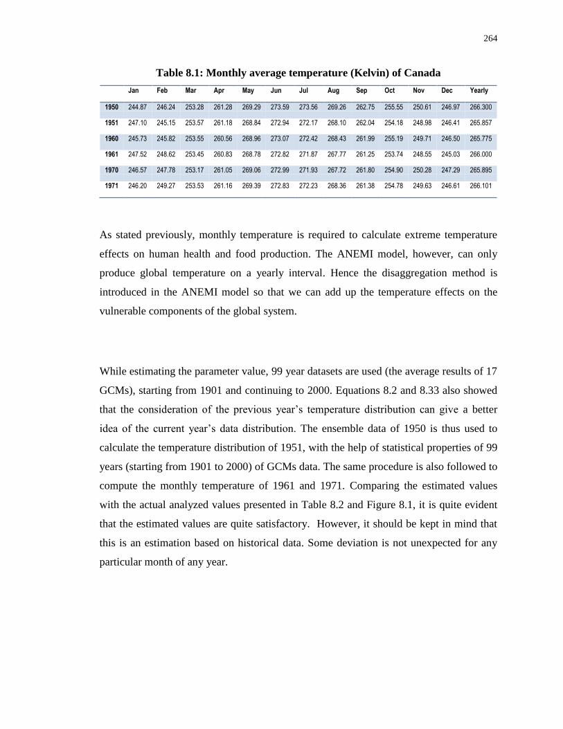
264

Table 8.1: Monthly average temperature (Kelvin) of Canada

Jan Feb Mar Apr May Jun Jul Aug Sep Oct Nov Dec Yearly

1950 244.87 246.24 253.28 261.28 269.29 273.59 273.56 269.26 262.75 255.55 250.61 246.97 266.300

1951 247.10 245.15 253.57 261.18 268.84 272.94 272.17 268.10 262.04 254.18 248.98 246.41 265.857

1960 245.73 245.82 253.55 260.56 268.96 273.07 272.42 268.43 261.99 255.19 249.71 246.50 265.775

1961 247.52 248.62 253.45 260.83 268.78 272.82 271.87 267.77 261.25 253.74 248.55 245.03 266.000

1970 246.57 247.78 253.17 261.05 269.06 272.99 271.93 267.72 261.80 254.90 250.28 247.29 265.895

1971 246.20 249.27 253.53 261.16 269.39 272.83 272.23 268.36 261.38 254.78 249.63 246.61 266.101

As stated previously, monthly temperature is required to calculate extreme temperature

effects on human health and food production. The ANEMI model, however, can only

produce global temperature on a yearly interval. Hence the disaggregation method is

introduced in the ANEMI model so that we can add up the temperature effects on the

vulnerable components of the global system.

While estimating the parameter value, 99 year datasets are used (the average results of 17

GCMs), starting from 1901 and continuing to 2000. Equations 8.2 and 8.33 also showed

that the consideration of the previous year‘s temperature distribution can give a better

idea of the current year‘s data distribution. The ensemble data of 1950 is thus used to

calculate the temperature distribution of 1951, with the help of statistical properties of 99

years (starting from 1901 to 2000) of GCMs data. The same procedure is also followed to

compute the monthly temperature of 1961 and 1971. Comparing the estimated values

with the actual analyzed values presented in Table 8.2 and Figure 8.1, it is quite evident

that the estimated values are quite satisfactory. However, it should be kept in mind that

this is an estimation based on historical data. Some deviation is not unexpected for any

particular month of any year.

265

Figure 8.1: Monthly temperature comparison between analyzed and simulated data

Table 8.2: Comparison of the average temperature (Kelvin), Canada

Year Jan Feb Mar Apr May Jun Jul Aug Sep Oct Nov Dec

1951

Analyzed 247.10 245.15 253.57 261.18 268.84 272.94 272.17 268.10 262.04 254.18 248.98 246.41

Simulated 246.38 247.97 253.04 261.05 268.83 273.74 273.08 269.25 262.40 254.40 248.66 245.78

1961

Analyzed 247.52 248.62 253.45 260.83 268.78 272.82 271.87 267.77 261.25 253.74 248.55 245.03

Simulated 247.09 247.54 253.12 260.96 268.63 273.14 272.56 268.98 262.08 254.34 249.24 246.71

1971

Analyzed 246.20 249.27 253.53 261.16 269.39 272.83 272.23 268.36 261.38 254.78 249.63 246.61

Simulated 247.87 249.28 253.57 261.14 268.51 272.91 272.10 268.50 261.89 254.31 249.57 247.20

240

250

260

270

280

290

300

220

230

240

250

260

270

280

Jan Feb Mar Apr May Jun Jul Aug Sep Oct Nov Dec

Tem

per

atu

re (

kel

vin

) in

19

51

Tem

per

atu

re (

kel

vin

) in

19

61

Month

Monthly Temperature Comparison

1961_analysed

1961_simulated

1951_analysed

1951_simulated

266

CHAPTER 9

9 CONCLUSIONS

Climate policy plays a key role in most integrated assessment models. A model should

therefore be capable of simulating the results of a proposed climate policy. In order to do

so, it is important that a model utilize an optimization procedure and have an energy

supply sector that takes into account the effects of non-renewable resource depletion.

This is what the ANEMI model version 2 does. Other integrated assessment models have

likewise utilized an optimization procedure and have incorporated energy sectors,

including FREE (Fiddaman, 1997; Fiddaman, 2002), TARGETS (Rotmans and de Vries,

1997), MESSAGE (Messner and Strubegger, 1995), and RICE (Nordhaus and Boyer,

2000). We can thus compare our ideas and the results of the ANEMI version 2 with these

previous models.

The ANEMI model has been developed and implemented on the global scale for the

study of ―Analyzing Behaviour of the Social-Energy-Economy-Climate System.‖ As it

combines a system dynamics-based simulation with a non-linear optimization procedure,

it can be described as a computer-based system hybrid model. It has a projection horizon

up to 2100. It provides an inclusive portrait of energy supply resources and technologies,

as well as a detailed picture of energy demand across several sectors. In the global

version of the model, it projects production, consumption, GDP and energy price. In the

regional version it is additionally able to produce import and export projections.

The model utilizes a one-period nonlinear optimization program for the energy–economy

sector, while a part of this sector is going through the simulation process. Similar to the

MESSAGE model (Messner and Strubegger, 1995), the ANEMI optimization process is

267

subject to constraints such as the availability of primary energy resources, the evolution

of energy conversion technologies and a set of useful energy demands in different end-

use sectors. The model calculates an optimal and feasible energy supply-technology mix

that requires the least total costs and meets a given useful or final energy demand.

This Chapter presents the methodology, algorithms and model results produced in

Chapters 3-8. The model results are applied on both global and local (Canada) scales.

First, the performance of the ANEMI version 2 and ANEMI_CDN model are evaluated

based on the available observational data. Then, the results of long term future simulation

under various policy scenarios are discussed in order to explore the consequences they

would have on the rest of the variables. Such experimentation aims to conceptualize the

impact of climate change on our socio-economic environment. Next, the methodology

and algorithm for the disaggregation modelling, as well as the embedded optimization

within the simulation scheme, are presented. Lastly, in conclusion, I briefly indicate the

future possibilities of expanding the robustness and scope of the ANEMI model in

capturing the future consequences of climate change on the social-energy-economy-

climate system.

9.1 Representation of the Past

The overall objective of this research is to represent our social-energy-economy-climate

system through ANEMI model development.

The first problem I confronted was how closely the ANEMI model could represent the

real world situation after the inclusion of new sectors and feedbacks.

268

This version of the ANEMI model (ANEMI version 2 and ANEMI_CDN) incorporates

three new major sectors (food production, population, and energy-economy) making it a

nine-sectoral model. The ANEMI model version 1.2 also contained population, energy,

and economy sectors in much simpler form. In the ANEMI version 2, they were

discarded and replaced with much more sophisticated representations. Hence we treat

these latter forms as new sectors. Other sectors have also been modified to a small extent.

For example, water quality and climate have incorporated different dilution requirements

based on their use, as well as radiative forcing from all GHGs, not only CO2 like in the

first version of ANEMI. The rest of the sectors have been subject to minor modifications.

As presented in Chapter 4, the global form of the ANEMI model version 2 produced

satisfactory results when compared to historical observations of water use, sea-level rise,

global population, CO2 emissions from the energy production, atmospheric CO2

concentration, GDP, net primary productivity, and global surface temperature. These

tested variables respectively represent most of the model‘s sectors. Thus, the satisfactory

comparison of our results and the historical data indicates the exactness, reliability and

improved formulations of the ANEMI version2 model.

In Chapter 6, we carried out a detailed comparative analysis of the regional ANEMI

model (ANEMI_CDN) in both graphical and tabular form. Water use for different types

of activities (domestic, agricultural, and industrial), land-use change (specifically, forest

and cultivable land), and per capita GDP were compared with the historical data. In the

case of the ANEMI_CDN model, the number of representing variables was less than the

global version. This is because many observations are simply not available on a regional

scale. (The climate and carbon sectors thus remained on a global scale and have already

been verified in Chapter 4.) Nevertheless, the comparison results prove the reliability of

the ANEMI_CDN, with acceptable deviations.

269

Therefore, both the ANEMI version 2 and the ANEMI_CDN perform satisfactorily and

are capable of handling different policy scenarios related to climate change.

9.2 How the Future May Look Under Various Policy Choices

As stated above, the first problem I confronted was how closely the ANEMI model could

represent the current situation of the social-energy-economy-climate system after the

inclusion of new sectors and feedbacks. The second problem concerned how the model

would represent the future behavior of the system, and how the state variables from the

different sectors would change under different climate-related risk mitigation policies.

This second problem immediately raised a further question: namely, whether one and the

same policy can work on both the global and regional scales. It was determined that some

policies that would work on the global scale would not be as effective on the regional

scale (i.e., in Canada).

When policy makers formulate their policies, they must assume various constraints

relevant to acceptable climate change impacts. A good climate policy demands the best

possible understanding of climate change and its subsequent impact on human life. While

it is almost impossible to find or develop a model that is capable of providing everything

accurately, an integrated assessment model must be able to provide credible output. The

ANEMI version 2 and ANEMI_CDN are designed to provide the most accurate and

credible results possible concerning the long-term impacts of policies on the social-

energy-economy-climate system. In this research we have selected three sets of

run/policy for both the global and regional (Canada) versions of the ANEMI model

experiment. These policy scenarios respond to real concerns of participating policy

makers, even though they do not include the real data and the policy implementation

timeframe. The three policy simulation results presented in the following subsections are

thus based on certain assumptions that we have used in this research to test the model.

270

9.2.1 Carbon Tax Implementation

One of the policy options that we explored was the implementation of a carbon tax in

2012. In this scenario, the carbon tax is presumed to be slowly ramped up to $100 per

tonne of CO2 emissions over the next 30 years. In Chapters 4 and 6, the carbon tax shows

a considerable influence on energy production, because fossil fuel based energy enjoys

the lion‘s share of total energy production. As the initial consumption declines, so the

reserves decline more slowly, ensuring more reserves in the future. Such decline also

lowers the fossil fuel based CO2 emissions, as it does the atmospheric temperature. Since

temperature is a directly related factor in sea-level rise, the latter also shows a lower

value. These favourable changes result in a more environmentally friendly situation that

subsequently invites an increase in population and thus more demand for food and water.

To meet this growing demand, more land area is required to be converted to irrigated

area. This leads to increased pressure on available water resources with respect to water

quantity and quality, which can be defined as water-stress. Increased water-stress works

as a negative feedback for further growth and leads to a more stable system. However,

with the introduction of carbon capture and storage technology, energy consumption will

slightly increase.

9.2.2 Increased Water Consumption

We also examined a 15% increase in water consumption in relation to other water uses,

so as to meet the growing water demand related to climate change. Such an increase in

consumption lowers the available surface water, resulting in a roughly 6% increase in

water-stress. The most affected sector in this case would be agriculture which could lose

more than 5% of its regular production. An increase in water-stress and a decrease in

food production would together threaten human average life expectancy. The population

would thus be expected to drop by 7.5%. The GDP would likewise drop, but only

nominally. With the reduced population, CO2 production from the burning of fossil fuel

decreases. However, there is little noticeable change in atmospheric temperature, since

271

the reduced amount of CO2 from the atmosphere is insignificant compared to total GHGs

equivalent.

Since Canada has the world‘s largest reserve of fresh water resources and a small

population, a 15% increase in water consumption hardly changes the total water reserve.

Nor does it introduce significant water-stress. As the water-stress remains within

tolerable range (0.4) till the end of this century, the ANEMI_CDN model shows the

ability of Canada‘s water resources to meet the extra demand with almost no negative

consequences on any of the model sectors. In this, it significantly differs from the global

model.

9.2.3 Increased Food Production

This policy scenario tests the impact of redistributing land-use, by converting 15% land

from forest to agriculture. The simulation results of Chapter 4 show that this expansion of

agricultural land is not able to increase food production in the long run. Rather, total food

production declines on the global scale. Both the extra irrigation demands from the newly

converted land and the increased population (at the initial stage) put great pressure on the

scarce water resources, increasing the water-stress beyond the tolerable range. Such a

stressful condition hampers food production, human life expectancy, and so on.

Moreover, even as the population declines, CO2 emissions continue to increase due to

land conversion (forest cutting/burning). Still, such an increase in CO2 emissions is not

able to increase the radiative forcing noticeably. So the atmospheric temperature and sea-

level rise remains almost unchanged.

The ANEMI_CDN model shows that a 15% land conversion leads to a roughly 13%

increase in food production. At the global scale, however, the initial increase is around

1% and then declines. The results can be explained by the sufficient availability of water

272

resources in Canada, which keeps the water-stress just below the threshold level.

Surprisingly, even with high per capita food production the life expectancy remained

almost same, probably because in general the Canadian population is already well-off.

Hence the further increase in per capita food production does not change anything except

total food production and water consumption.

9.3 Optimization Simulation of ANEMI Model

One of the research objectives of climate science in general and this thesis in particular is

to derive better policy and decision-making approaches to energy consumption while

keeping an eye on greenhouse gas emissions. By itself, the application of an optimization

procedure to a complex problem remains somewhat limited, since an efficient

optimization always requires the simplified representation of the problem to be

convergent. Such simplification can make it difficult to determine the accuracy of both

the assumptions and the results, and this holds back the actual implementation of

technically optimal solutions. In such a situation, a hybrid simulation-based optimization

can retain a sufficiently detailed, realistic description.

This research used simulation-based optimization as an integrated approach. We searched

the optimal setting of input parameters to minimize the simulation cost and to maximize

the advantages of simulation process. We embedded non-linear systems of equations for

the energy-economy sector of both the ANEMI version 2 and ANEMI_CDN, in order to

implement the market clearance mechanism, which utilizes the trust-region method

(Conn et al., 2000) with the dogleg algorithm (Fletcher and Powell, 1963).

The advantage of this method is that it is computationally efficient and probably

convergent (since it only has to solve one linear system of equations per iteration). It is

therefore more robust that the Gauss-Newton method. Furthermore, this method improves

273

the protection level by avoiding approximations or decompositions. At the same time, it

can include correlations among itineraries or correlations. Moreover, because of its

continuous nature, the ANEMI model bypasses the difficulties of working with finite-

difference estimates. With respect to computation time, robustness and model results

(presented in Chapters 3 to 6), the methodology of integrating an optimization scheme

within a system dynamics simulation environment works reasonably well, with only

minor difficulties. Finally, this integrated approach successfully showed its efficacy with

respect to computing the large, real-world networks with its simple implementation

procedure.

Therefore, the idea of embedding an optimization scheme in a simulation framework of a

feedback-based system dynamics model augments the applicability of the system

dynamics method in supporting the decision-making process in the context of the socio-

energy-economic-climate system.

9.4 Regionalization

In assessing the potential effects of climate change on the climatic system, and on water

resources in particular, it is important to incorporate predictions of future climatic trends

into hydrologic planning models (Firor et al., 1996). IPCC has been evaluating the impact

of global warming through global circulation models (GCMs). Many studies over the last

century have established different techniques while resolving the differences in both the

spatial and the temporal scales. Kim et al. (1984) used orthogonal functions and linear

regression to generate intermediate temperature and precipitation based on 30 years of

historical data. However, such techniques are not capable of preserving a requisite

statistical character (standard deviation, skewness coefficient and lag-one correlation

coefficient and so on).

274

The ANEMI version 2 and ANEMI_CDN both follow the approach of Salas et al. (1980),

who present a disaggregation model that generates time-series based on available

historical data, without sacrificing the statistical properties of standard deviation,

skewness coefficient and lag-one correlation coefficient. This disaggregation modelling

approach is verified by comparing simulated monthly temperature (generated from the

yearly average temperature) with the ensemble GCM monthly temperature. The

comparison indicates that the simplified disaggregation method could efficiently

reproduce average monthly temperature from the yearly average value.

This modelling approach proves its ability to produce reliable monthly and regional time-

series from the yearly global GCMs output (see Chapter 7). The same approach can be

applied to generate further local and weekly time series data. This disaggregation

technique thus exhibits a good potential in resolving the incongruity in both spatial and

temporal resolution between GCMs and the ANEMI_CDN model. It thereby facilitates

the capture of the hydrologic consequences of climate change.

9.5 Adjudication

We have developed the ANEMI version 2 and ANEMI_CDN as comprehensive system

dynamics simulation-based integrated assessment models with embedded optimization

schemes for analyzing the behaviour of the social-energy-economy-climate system in

order to advance climate science research and policy analysis. The power of an integrated

assessment model like ANEMI (ANEMI version 2, ANEMI_CDN) is shown in its

capacity to handle a multifaceted array of relevant constituent knowledge that is linked

across multiple sectors. Still, the ANEMI model cannot be used for all assessments. It is

built on a rich feedback linkage to provide near realistic representations, thereby

influencing the level of mitigation with the policies. More importantly, with the

introduction of the market clearance mechanism within the energy-economy sector, the

275

ANEMI model (ANEMI version 2, ANEMI_CDN) has become a general equilibrium

system dynamics simulation based integrated assessment model; and this makes it unique

in the field of integrated assessment modelling of climate change study.

9.6 Recommendations for Future Research

Integrated assessment modelling has the unique ability to unite the natural and social

sciences. In the last twenty years, it has developed to become an increasingly important

tool for climate change research.

The current energy-economy sector of the ANEMI model (ANEMI version 2,

ANEMI_CDN) may require changes in some of the key parameters. For one thing, the

approach taken in the modelling of electric energy production is myopic, as the simulated

investment decisions do not consider the future of the process. Moreover, the model

tends to break down when the total cost of electricity production for the fossil fuel type

rises exponentially, due to the inability of capital stock to adjust optimally. The inclusion

of the optimal capital stock adjustment mechanism in combination with the forward

looking behavior could therefore be the next step to have a more robust energy-economy

sector of the ANEMI model. The introduction of a ‗back-stop‘ technology (Kemfert,

2002), where at a threshold price a greenhouse gas free energy source could become

more cost-effective, could prove a very clever idea.

Future research should focus on investment decisions for the energy-economy sector, as

well as the addition of capital to electricity production. In case of regionalization, the rest

of the world (ROW) should, considering the data availability, be disaggregated into more

regions, preferably 11: USA, EU, Former USSR & E. Europe, China, Latin America, N.

Africa & Middle East, Sub-Saharan Africa, Indian Subcontinent, Japan & Asian Tigers,

276

SE Asia, and Oceania. In connection to such regionalization, the climate damage function

and a few other parameters need to be determined. Moreover, there is always room in the

ANEMI model to experiment with the implementation of new policy recommendations.

The land-use sector of the current version of the ANEMI model (ANEMI version 2,

ANEMI_CDN) is not sophisticated enough. The aggregate causes of land-use change

remain unclear. Experimentation with different drivers, including population, economic

output, and climatic effects could help in finding the missing links with the possible land-

use change pattern. An improvement in the understanding of both the causes and the

effects of the land-use change process at the global scale should therefore make the

results more convincing.

Water is the most valuable resource on the globe. It is the most basic need of human

survival, and it thus determines the overall prospects of a country. Unfortunately such an

important resource is not abundant all over the world. Indeed most areas are under water-

stressed conditions. Therefore water conservation is no longer an option. Anything scarce

and in demand commands a price; this is one of the basic principles of economics. Two

particular areas of water policy that has become increasingly subject to pricing principles

are those of public water supply and wastewater services. Water sectors in the ANEMI

model (ANEMI version 2, ANEMI_CDN) are not linked with the economy sector, so

performing water pricing policy endogenously is not a plausible solution. The

implementation of the market clearing mechanism for the water sectors will therefore

definitely guide the model along the path of environmental sustainability.

We have implemented the ANEMI model (ANEMI version 2, ANEMI_CDN) to

investigate a limited number of policy scenarios derived through discussion among a

narrow group of participating decision makers. But while this current group of partners

have provided important insights, further initiatives need to be considered. Many other

277

important questions raised in the course of this research remain unanswered. It is

therefore necessary to expand the group of partners across different departments in order

to accommodate a broader range of interests, according to a systems view of government.

In addition, further research on the international climate change related policy is required

to assess the consequences in global context.

278

REFERENCES

Achour, Mehdi, Friedhelm Betz, Antony Dovgal, Nuno Lopes, Hannes Magnusson, Georg

Richter, Damien Seguy, Jakub Vrana, (2011). PHP Manual. Available at:

http://www.php.net/manual/en/index.php, last accessed Oct. 01, 2011.

Ahmad, S., S. P. Simonovic, (2004). Spatial system dynamics: new approach for simulation of

water resources systems. J Comput Civ Eng, 18(4): 331–340.

Ahmad, S., S. P. Simonovic, (2006). An intelligent decision support system for management of

floods. Water Resour Manage, 20(3): 391–410.

Akhtar, M. K., S. P. Simonovic, J. Wibe, J. MacGee, and J. Davies, (2011). An integrated system

dynamics model for analyzing behaviour of the social-energy-economic-climatic system: User‘s

Manual. Water Resources Research Report no. 076, Facility for Intelligent Decision Support,

Department of Civil and Environmental Engineering, London, Ontario, Canada, 161 pages.

Alcamo J., R. Shaw, and L. Hordijk (eds), (1990). The RAINS Model of Acidification. Science

and Strategies in Europe. Dordrecht, Netherlands: Kluwer Academic Publishers.

Alcamo, J. and T. Henrichs (2002) Critical regions: A model-based estimation of world water

resources sensitive to global changes. Aquatic Sciences, 64: 352-362.

Alcamo, J., G. J. J. Kreileman, J. C. Bollen, G. J. van den Born, R. Gerlagh, M. S. Krol, A. M. C.

Toet and H. J. M. de Vries. (1996).Baseline scenarios of global environmental change. Global

Environmental Change, 6: 261-303.

Alcamo, J., G. J. J. Kreileman, M. S. Krol and G. Zuidema. (1994). Modeling the global society-

biosphere-climate system: Part 1: Model description and testing. Water, Air and Soil Pollution,

76: 1-35.

Alcamo, J., P. Döll, T. Henrichs, F. Kaspar, B. Lehner, T. Rösch and S. Siebert. (2003a).

Development and testing of the WaterGAP 2 global model of water use and availability.

Hydrologic Sciences Journal, 48: 317-337.

Alcamo, J., P. Döll, T. Henrichs, F. Kaspar, B. Lehner, T. Rösch and S. Siebert. (2003b). Global

estimates of water withdrawals and availability under current and future "business-as-usual"

conditions. Hydrologic Sciences Journal, 48: 339-348.

Alcamo, Joseph, (1994). Preface. Water, Air, & Soil Pollution, 76: 1-2.

Almeder, C., and P. Margaretha, (2007). A Hybrid Simulation Optimization Approach for Supply

Chains- Multimethod Simulation Software Tool AnyLogic. EUROSIM 2007, Ljubljana, Slovenia.

Amodeo, L., C. Prins, and D.R. Sánchezin, (2009). Comparison of Metaheuristic Approaches for

Multi-objective Simulation-Based Optimization in Supply Chain Inventory Management.

Applications of Evolutionary Computing EvoWorkshops 2009, Lecture Notes in Computer

Science, 5484: 798-807.

279

AQUASTAT, (2010). FAO's Information System on Water and Agriculture, Food and

Agriculture Organization of the Unites Nations. Available

fromhttp://www.fao.org/nr/water/aquastat/main /index.stm, last accessed December 12, 2010.

Arnell, N. W. (1999a). A simple water balance model for the simulation of streamflow over a

large geographic domain. Journal of Hydrology, 217: 314-335.

Arnell, N. W. (1999b). Climate change and global water resources. Global Environmental

Change, 9: S31-S49.

Atjay, G. L., P. Ketner and P. Duvigneaud. (1979). Terrestrial primary production and phytomass,

in The Global Carbon Cycle, edited by B. Bolin, E. T. Degens, S. Kempe and P. Ketner, pp. 129-

181, John Wiley and Sons, Chichester, U.K.

Azadivar, F., T. Truong, K. D. E. Stokesbury, and B. J. Rothschild, (2002). Simulation based

optimization in fishery management. Proceedings of the 2002 Winter Simulation Conference.

Citeseer.

Barlas, Y., (1996). Formal aspects of model validity and validation in system dynamics. System

Dynamics Review, 12(3): 183–210.

Barnett, B., (1973). A System Dynamics Model of an Oilfield's Development, Ph.D. Thesis,

University of Bradford.

Bashi-Azghadi, S. N., and R. Kerachian, (2010). Locating monitoring wells in groundwater

systems using embedded optimization and simulation models. Sci Total Environ, 408(10):2189-

2198.

Bates, B.C. , Z.W. Kundzewicz, S. Wu and J.P. Palutikof, Eds. (2008). Climate Change and

Water, Technical Paper VI of the Intergovernmental Panel on Climate Change, IPCC Secretariat,

Geneva, 210 pp.

Berkofsky, L., D. Faiman, J. Gale, (1981). Settling the Desert. New York: Gordon and Breach

Science Publishers.

Berthelot, M., P. Friedlingstein, P. Ciais, P. Monfray, J. L. Dufresne, H. Le Treut and L.

Fairhead, (2002). Global response of the terrestrial biosphere to CO2 and climate change using a

coupled climate-carbon cycle model. Global Biogeochemical Cycles, 16(4), 1084,

doi:10.1029/2001GB001827.

Better, M., F. Glover, G. Kochenberger, and H. Wang, (2008). Simulation Optimization:

Applications in Risk Management. International Journal of Information Technology & Decision

Making, 7(4): 571-587.

Bhattacharjya, R. K., and B. Datta, (2005). Optimal Management of Coastal Aquifers Using

Linked Simulation Optimization Approach. Water Resources Management, 19(3): 295-320.

Bowden, M. J., J. M. Glennie, (1986). Integrated water resource management on the central

plains: the need for irrigation. N Z Agric Sci, 20(1):18–22.

Bowe, TR., WD. Dapkus, and JB. Patton, (1990). Markov models. Energy, 15: 661–676.

280

Box, G. E. P., and D. R. Cox, (1964). An analysis of transformations, Journal of the Royal

Statistical Society, Series B (26): 211-252.

Box, G.E.P., and G. M. Jenkins, (1970). Time Series Analysis: Forecasting and Control, Holden-

Day Inc, San Francisco.

Brohan, P., J. J. Kennedy, I. Harris, S. F. B. Tett, and P. D. Jones (2006). Uncertainty estimates in

regional and global observed temperature changes: A new data set from 1850, Journal of

Geophysical Research, 111, D12106, doi:10.1029/2005JD006548

Buras, N. (1972). Scientific Allocation of Water Resources, Water Resources Development and

Utilization –A Rational Approach. American Elsevier. New York.

Burn, D. H. (1997), Catchments similarity for regional flood frequency analysis using seasonality

measures, J. Hydrol., 202: 212–230.

Calvin, K., J. Edmonds, B. Bond-Lamberty, L. Clarke, S.H. Kim, P. Kyle, S.J. Smith, A.

Thomson, and M. Wise (2009). 2.6: Limiting climate change to 450 ppm CO2 equivalent in the

21st century. Energy Economics, 31(Supplement 2): S107-S120.

Camara, A. S., M. G. Viegas, A. Amaro, (1986). Interfacing system dynamics and multiobjective

programming for regional water resources planning. Ann Reg Sci, 20(3):104–113.

Capros, P., L. Mantzos, D. Kolokotsas, N. Ioannou, T. Georgakopoulos, A. Filippopoulitis, Y.

Antoniou, (1998). The PRIMES Energy System Model–Reference Manual. National Technical

University of Athens. Document as peer reviewed by the European Commission, Directorate

General for Research.

Cartwright, L., J. Connor, (2003). Collaborative water supply planning: a shared vision approach

for the Rappanhannock Basin. In: Proceedings of the 2003 UCOWR meeting, Universities

Council on Water Resources, Washington, DC.

Center for International Earth Science Information Network (CIESIN). 1995. Thematic Guide to

Integrated Assessment Modeling of Climate Change [online]. Palisades, NY: CIESIN. Available

at http://sedac.ciesin.columbia.edu/mva/iamcc.tg/TGHP.html, last accessed Sept. 20, 2011.

Cetinkaya, C.P., O. Fistikoglu, K. Fedra, and N. B. Harmancioglu, (2008). Optimization methods

applied for sustainable management of water-scarce basins. Journal of Hydroinformatics, 10: 69–

95.

Chahine, Moustafa T., ( 1992). The Hydrologic Cycle and Its Influence on Climate, Review

Article, Nature, 359: 373 – 380.

Chapagain, AK, A.Y. Hoekstra, H.H.G. Savenije, and R. Gautam, (2006). The water footprint of

cotton consumption: An assessment of the impact of worldwide consumption of cotton products

on the water resources in the cotton producing countries, Ecological Economics, vol. 60, no. 1,

pp. 186-203.

Chedid, R., T. Mezher, and C. Jarrouche, (1999). A fuzzy programming approach to energy

resource allocation. Internal Journal Energy Research, 23(4), 303–317.

281

Clarke, L., J. Edmonds, H. Jacoby, H. Pitcher, J. Reilly, R. Richels, (2007). Scenarios of

Greenhouse Gas Emissions and Atmospheric Concentrations. Sub-report 2.1A of Synthesis and

Assessment Product 2.1 by the U.S. Climate Change Science Program and the Subcommittee on

Global Change Research. Department of Energy, Office of Biological & Environmental

Research, Washington, DC., USA, 154 pp.

Climaco, J., A. Henggeler, M. A. Gomes, and A. A. Traca, (1995). A Multiple Objective Linear

Programming Model for Power Generation Expansion Planning. International Journal of Energy

Research, 19: 419-432.

CLIMAP, (2011, June 01). General Circulation Models (GCMs), http://climap.net/general-

circulation-models-gcms, last accessed September 01, 2011.

Cohen, S., T. Neale, (2006). Participatory integrated assessment of water management and

climate change in the Okanagan Basin, British Columbia. Final report, Environment Canada and

University of British Columbia.

Conn, A. R., N. I. M. Gould, and P. L. Toint, (2000). Trust-Region Methods. Philadelphia, PA:

SIAM.

Connor, J., L. Cartwright, K. Stephenson, (2004). Collaborative water supply planning: a shared

vision approach for the Rappahannock Basin in Virginia. In: Sehlke G, Hayes DF, Stevens DK

(eds) Proceedings of the 2004 world water and environmental resources congress. Salt Lake

City, Utah, USA, pp 1–9, 27 June–1 July 2004. Environmental and Water Resources Institute of

The American Society of Civil Engineers. doi:10.1061/40737(2004)323

Cosgrove, W. J. and F. R. Rijsberman. (2000). World Water Vision: Making Water Everybody's

Business. Earthscan Publications Ltd., London, U.K.

Cowpertwait, P. S. P. (1994), A generalised point process model for rainfall, Proc. R. Soc., 447:

23– 37.

Cowpertwait, P. S. P., C. G. Kilsby, and P. E. O‘Connell (2002), A spacetime Neyman-Scott

model of rainfall: Empirical analysis of extremes, Water Resour. Res., 38(8): 1131,

doi:10.1029/2001WR000709

Cox, P. M., R. A. Betts, C. D. Jones, S. A. Spall and I. J. Totterdell, (2000). Acceleration of

global warming due to carbon-cycle feedbacks in a coupled climate model. Nature, 408: 184-187.

doi:10.1038/35041539

Coyle, R. G., (1970). A Dynamic Model of the Copper Industry-some preliminary results. Proc.

9th International Conference on Computers in the Mineral Industry, 53-60.

Coyle, R. G., (1972). Dynamic Control of a Mining Enterprise. Proc. 10th International Conf. on

Computers in the Mineral Industry, 357-360.

Coyle, R. G., (1989). System dynamics: The next ten years. In Flood, R. L., Jackson, M. C., and

Keys, P. (eds.), Systems Prospects: The Next Ten Years of Systems Research, Plenum Press, New

York.

282

Cramer, W., A. Bondeau, F. I. Woodward, I. C. Prentice, R. A. Betts, V. Brovkin, P. M. Cox, V.

Fisher, J. A. Foley, A. D. Friend, C. Kucharik, M. R. Lomas, N. Ramankutty, S. Sitch, B. Smith,

A. White and C. Young-Molling, (2001). Global response of terrestrial ecosystem structure and

function to CO2 and climate change: Results from six dynamic vegetation models. Global

Change Biology, 7: 357-373.

Cramer, W., D. W. Kicklighter, A. Bondeau, B. Moore, C. Churkina, B. Nemry, A. Ruimy and A.

L. Schloss, (1999). Comparing global models of terrestrial net primary productivity (NPP):

overview and key results. Global Change Biology, 5(Suppl. 1): 1-15.

Crawford, N. H., R. K. Linsley, (1966). Digital simulation in hydrology: Stanford Watershed

Model IV. Technical Report 39, Civil Engineering Deptartment, Stanford University, California.

Da Cunha, L.V., (1989). Water resources situation and management in the EEC. Hydrogeology,

2:57–69

Dabrowski, J.M., K. Murray, P.J. Ashton, J.J. Leaner (2009). Agricultural impacts on water

quality and implications for virtual water trading decisions. Ecological Economics, 68: 1074-

1082.

Dasgupta, S., B. Laplante, C. Meisner, D. Wheeler, and J. Yan, (2009). The impact of sea level

rise on developing countries: a comparative analysis, Climatic Change, 93:379–388.

Dash, D.P., (1994). System Dynamics: Changing Perspectives, Systems Practice, 7(1): 87-98.

Davide, F., M. Riccardo, R. Michela, R. Mauro, S. Roberto, and T. Angela, (2004). Optimizing

forest biomass exploitation for energy supply at a regional level, Biomass and Bioenergy, 26: 15–

25.

Davies, E. G. R. (2007). Modelling Feedback in the Society-Biosphere-Climate System. Ph.D.

thesis. Department of Civil and Environmental Engineering, the University of Western Ontario,

London, Ontario, Canada.

Davies, E. G. R. and S. P. Simonovic, (2008). An Integrated System Dynamics Model for

Analyzing Behaviour of the Social-Economic-Climatic System: Model Description and Model

Use Guide. Water Resources Research Report no. 059, Facility for Intelligent Decision Support,

Department of Civil and Environmental Engineering, London, Ontario, Canada, 233 pages.

ISBN: (print) 978-0-7714-2679-7; (online) 978-0-7714-2680-3.

Davies, E. G. R. and S. P. Simonovic, (2009). Energy Sector for the Integrated System Dynamics

Model for Analyzing Behaviour of the Social-Economic-Climatic Model. Water Resources

Research Report no. 063, Facility for Intelligent Decision Support, Department of Civil and

Environmental Engineering, London, Ontario, Canada, 191 pages. ISBN: (print) 978-0-7714-

2712-1; (online) 978-0-7714-2713-8.

Davies, Evan G. R. and S. P. Simonovic, (2010). ANEMI: A new model for integrated

assessment of global change. Interdisciplinary Environmental Review, 11(2/3): 127-161.

Davies, E. G. R. and S. P. Simonovic, (2011) Global water resources modeling with an integrated

model of the social-economic-environmental system. Advances in Water Resources, 34(6): 684-

700.

283

DeCarolis, Joseph F., (2011). Using modeling to generate alternatives (MGA) to expand our

thinking on energy futures. Energy Economics, 33: 145–152.

Den Exter, K., (2004). Integrating environmental science and management: the role of system

dynamics modelling. PhD thesis, CRC Sustainable Tourism School of Environmental Science

andManagement, Southern Cross University, Queensland, Australia.

Den Exter, K., A. Specht, (2003). Assisting stakeholder decision making using system dynamics

group model-building. In: Extending extension: beyond traditional boundaries, methods and ways

of thinking!. Proceedings of the 2003 APEN national forum, Hobart.

Deng, G., (2007). Simulation-based optimization. Ph.D. thesis, University of Wisconsin, 2007.

Döll, P., (2002). Impact of climate change and variability on irrigation requirements: A global

perspective. Climatic Change, 54: 269-293.

Dowlatabadi, H., (2000). Bumping against a gas ceiling, Climatic Change, 46(3): 391–407.

Dowlatabadi, H., and M. G. Morgan, (1993a). A Model Framework for Integrated Studies of the

Climate Problem, Energy Policy, 21(3): 209-221.

Dowlatabadi, H., and M. G. Morgan, (1993b). Integrated Assessment of Climate Change.

Science, 259(5103): 1813-1932

Dowlatabadi, H., and M. G. Morgan, (1995). A Model Framework for Integrated Assessment of

the Climate Problem, mimeo, Department of Engineering and Public Policy, Carnegie Mellon

University.

Dyson, B., and N. B. Chang, (2005). Forecasting municipal solid waste generation in a fast-

growing urban region with system dynamics modeling. Waste Management, 25: 669-679.

Edmonds, J., M. Wise, and C. MacCracken., (1994). Advanced Energy Technologies and Climate

Change: An Analysis Using the Global Change Assessment Model (GCAM), PNL-9798, UC-402.

Pacific Northwest Laboratory, Richland, WA 99352.

Edmonds, J., M. Wise, R. Sands, R. Brown, and H. Kheshgi, (1996b). Agriculture, Land-Use,

and Commercial Biomass Energy: A Preliminary Integrated Analysis of the Potential Role of

Biomass Energy for Reducing Future Greenhouse Related Emissions. PNNL-11155. Pacific

Northwest National Laboratories, Washington, DC.

Edmonds, J., Wise, M., Pitcher, H., Richels, R., Wigley, T., and MacCracken, C., (1996a). "An

Integrated Assessment of Climate Change and the Accelerated Introduction of Advanced Energy

Technologies: An Application of MiniCAM 1.0," Mitigation and Adaptation Strategies for

Global Change, 1(4):311-339.

Energy Information Administration (EIA), (2006). Official Energy Statistics from the U.S.

Government. U.S. Department of Energy, Washington, D.C. Available at

http://www.eia.doe.gov/emeu/international/contents.html, last accessed Oct. 21, 2010.

284

Energy Information Administration (EIA), (2008). Carbon Dioxide Emission Factors (1980 -

2006). U.S. Department of Energy, Washington, D.C. Available at

http://www.eia.doe.gov/oiaf/1605/ggrpt/excel/CO2_coeff.xls, last accessed July, 2011.

Environment Canada (EC), (October 08, 2008). Municipal Wastewater Status in Canada.

Available from http://www.ec.gc.ca/eu-ww/default.asp?lang=En&n=6E4ACEEE-1 , last accessed

October 01, 2011.

Erdem, A. S., and U. A. Sancarin, (2006). A Simulation Based DSS Design for Supply Chain

Management. Technology Management for the Global Future PICMET 2006 Conference, 6(c):

2741-2747.

European Union, (2007). The EU Water Framework Directive - integrated river basin

management for Europe. http://ec.europa.eu/environment/water/water-framework/index_en.html,

last accessed March 27, 2011.

Falkenmark, M., (2005). Water usability degradation – Economist wisdom or societal madness?

Water International, 30: 136-146.

Falkowski, P., R. J. Scholes, E. Boyle, J. Canadell, D. Canfield, J. Elser, , N. Gruber, K. Hibbard,

P. Hoegberg, S. Linder, F.T. Mackenzie, B. Moore III, T. Pedersen, Y. Rosenthal, S. Seitzinger,

V. Smetacek and W. Steffen, (2000). The global carbon cycle: A test of our knowledge of earth

as a system. Science, 290: 291-296.

FAO (2009). Global agriculture towards 2050, High Level Expert Forum - How to Feed the

World in 2050 Office of the Director, Agricultural Development Economics Division Economic

and Social Development Department, Rome, Italy. Available from

http://www.fao.org/fileadmin/templates/wsfs/docs/Issues_papers/HLEF2050_Global_Agriculture

.pdf, Last accessed May.30, 2011.

Fauresa, J. M., J. Hoogeveena, and J. Bruinsmab (2003). The FAO Irrigated Area Forecast for

2030, FAO, Rome, Italy. Available from http://www.anafide.org/doc/HTE%20125/125-3.pdf, last

accessed May.30, 2011.

Fedra, K., and N. B. Harmancioglu, (2005). A web-based water resources simulation and

optimisation system, in: D. Savic, G. Walters, R. King and A.-T. Khu (Eds.), Proc. of CCWI 2005

on Water Management for the 21st Century, Center of Water Systems, Univ. of Exeter., V(II):

167–172.

Fiddaman, T. S., (1997). Feedback complexity in integrated climate-economy models. Ph.D.

thesis. Alfred P. Sloan School of Management, Massachusetts Institute of Technology, Boston,

Massachusetts, U.S.A.

Fiddaman, T. S., (2002). Exploring policy options with a behavioral climate-economy model.

System Dynamics Review, 18: 243-267.

Firor, Susan E., Brad A. Finney, Robert WiIlis, and John A. Dracup, (1996). Disaggregation

Modeling Process for Climate Time Series, Journal of Water Resources Planning and

Management, 122(3): 205-212.

Fletcher, R., and M.J.D. Powell, (1963). A Rapidly Convergent Descent Method for

Minimization. Computer Journal, 6: 163-168.

285

Floros, N., and A. Vlachou, (2005). Demand and energy-related CO2 emissions in Greek

manufacturing: Assessing the impact of a carbon tax. Energy Economics, 27(3): 387-413.

Forrester, J. W., (1958). Industrial dynamics: A major breakthrough for decision makers. Harvard

Bus. Rev. 36: 37-66.

Forrester, J. W., (1961). Industrial Dynamics, MIT Press, Cambridge, Mass.

Forrester, J. W., (1987). Lessons from system dynamics modeling. System Dynamics Review,

3(2): 136–149.

Forrester, J. W., (1994). System dynamics, systems thinking and soft OR, System Dynamics

Review, 10(2): 245-256.

Forster, P. M. d. F., and J. M. Gregory. (2006). The climate sensitivity and its components

diagnosed from Earth radiation, Journal of Climate, 19: 39-52.

Foufoula-Georgiou, E., (1998). On scaling theories of space-time rainfall: Some recent results

and open problems, in Stochastic Methods in Hydrology, edited by O. Barndorff-Nielsen et al.,

pp. 25– 72, World Sci., Hackensack, N. J.

Fujino, J., R. Nair, M. Kainuma, T. Masui, Y. Matsuoka, (2006). Multi-gas mitigation analysis on

stabilization scenarios using AIM global model. Multigas Mitigation and Climate Policy. The

Energy Journal, Special Issue #3.

Geider, R. J., E. H. Delucia, P. G. Falkowski, A. C. Finzi, J. P. Grime, J. Grace, T. M. Kana, J. La

Roche, S. P. Long, B. A. Osborne, T. Platt, I. C. Prentice, J. A. Raven, W. H. Schlesinger, V.

Smetacek, V. Stuart, S. Satyendranath, R. B. Thomas, T. C. Vogelmann, P. Williams and F. I.

Woodward. (2001). Primary productivity of planet Earth: Biological determinants and physical

constraints in terrestrial and aquatic habitats. Global Change Biology, 7: 849-882.

Gleick, P. H. (2000a). The changing water paradigm: A look at twenty-first century water

resources development. Water International, 25: 127-138.

Gleick, P. H. (2000b). The world's water: the biennial report on freshwater resources. Island

Press, Washington, D.C., U.S.A.

Goldewijk, K. K., J. G. van Minnen, G. J. J. Kreileman, M. Vloedbeld and R. Leemans. (1994).

Simulating the carbon flux between the terrestrial environment and the atmosphere. Water, Air

and Soil Pollution, 76: 199-230.

Goodess, CM, C. Hanson, M. Hulme, T. J. Osborn, (2003). Representing climate and extreme

weather events in integrated assessment models: a review of existing methods and options for

development. Integr Assess, 4:145–171.

Goudriaan, J. and P. Ketner. (1984). A simulation study for the global carbon cycle, including

man's impact on the biosphere. Climatic Change, 6: 167-192.

Government of Canada, (2000). A Framework for Science and Technology Advice: Principles

and Guidelines for the Effective Use of Science and Technology Advice in Government Decision

Making (Ottawa), http://dsp-psd.pwgsc.gc.ca/Collection/C2- 500-2000E.pdf, last accessed July

16, 2011.

286

Groscurth, H. M., Th Bruckner, R. Kummel, (1995). Modelling of energy-services supply

systems. Energy, 20: 941–58.

Guo, H.C., L. Liu, G.H. Huang, G.A. Fuller, R. Zou, Y.Y. Yin, (2001). A system dynamics

approach for regional environmental planning and management: a study for the Lake Erhai Basin.

J Environ Manag, 61(1):93–111, January. doi:10.1006/jema.2000.0400

Gyasi-Agyei, Y., and G. Willgoose (1997), A hybrid model for point rainfall modelling, Water

Resour. Res., 33: 1699–1706.

Hamilton, H.R., (1969). Systems simulation for regional analysis: an application to river-basin

planning. MIT, Cambridge. ISBN: 0262080303

Hansen, J.E., D. Johnson, A. Lacis, S. Lebedeff, P. Lee, D. Rind, and G. Russell,( 1981). Climate

impact of increasing atmospheric carbon dioxide. Science, 213: 957-966,

doi:10.1126/science.213.4511.957.

Hansen, J.E., R. Ruedy, J. Glascoe, and Mki. Sato, (1999): GISS analysis of surface temperature

change. Journal of Geophysical Research, 104(D24): 30997-31022.

Hansen, J.E., R. Ruedy, Mki. Sato, M. Imhoff, W. Lawrence, D. Easterling, T. Peterson, and T.

Karl, (2001). A closer look at United States and global surface temperature change. Journal of

Geophysical Research, 106: 23947-23963.

Hansen, M.C., and B. Reed, (2000). A comparison of the IGBP DISCover and University of

Maryland 1km global land-cover products, International Journal of Remote Sensing, 21:1365–

1373.

Hare, W.L. (2009). ‗A Safe Landing for the Climate’, in Worldwatch Institute Into a Warming

World, State of the World Report 2009, pp. 13–29. New York: W.W. Norton & Co.

Harms, A. A., and T. H. Campbell, (1967). An extension to the Thomas- Fiering model for the

sequential generation of stream flow, Water Resour. Res., 3(3): 653–661.

Harremoes, P., R.K. Turner, (2001). Methods for integrated assessment. Reg Environ Change,

2:57–65.

Harvey, D., J.M.Gregory, M. Hoffert, A.Jain, M.Lal, R.Leemans, S.Raper, T.M.L.Wigley, and

J.de Wolde, (1997). An introduction to simple climate models used in the IPCC Second

Assessment Report. IPCC Technical Paper II, Intergovernmental Panel on Climate Change,

Geneva, Switzerland, 47pp.

Harvey, L. D. D. (2000). Box models of the terrestrial biosphere, in The Carbon Cycle, edited by

T. M. L. Wigley and D. S. Schimel, pp. 238-247, Cambridge University Press, Cambridge, U.K.

Harvey, L. D. D. and S. H. Schneider. (1985a). Transient climate response to external forcing on

100–10

4 year time scales. Part I: Experiments with globally averaged, coupled, atmosphere and

ocean energy balance models. Journal of Geophysical Research, 90(D1): 2191-2205.

Harvey, L. D. D. and S. H. Schneider. (1985b). Transient Climate Response to External Forcing

on 100–10

4 Year Time Scales. Part 2: Sensitivity Experiments With a Seasonal, Hemispherically

287

Averaged, Coupled Atmosphere, Land, and Ocean Energy Balance Model. Journal of

Geophysical Research, 90(D1): 2207–2222.

Harvey, L. D. D. and Z. Huang. (2001). A quasi-one-dimensional coupled climate-change

carbon-cycle model 1. Description and behaviour of the climate component. Journal of

Geophysical Research, 106(C10): 22339-22353.

Hastings, D.A. and P.K. Dunbar, (1998). Development and assessment of the Global Land One-

km Base Elevation Digital Elevation Model (GLOBE). International Society of Photogrammetry

and Remote Sensing, Archives, 32: 218-221.

Hay, L., G. McCabe Jr., D. Wolock, and M. Ayers (1992). Use of weather types to disaggregate

general circulation model predictions, Journal of Geophysical Research, 97(D3): 2781-2790.

Hay, L.E., G. J. Jr. McCabe, D.M. Wolock, and M.A. Ayers, (1992). Use of weather types to

disaggregate general circulation model predictions. J. Geophys. Res. 97(D3): 2781-2790.

Hijioka, Y., Y. Matsuoka, H. Nishimoto, M. Masui, and M. Kainuma, (2008). Global GHG

emissions scenarios under GHG concentration stabilization targets. Journal of Global

Environmental Engineering, 13: 97-108.

Hill, G.W., (1972). A Dynamic Model of Investment by the Chemical (and Petrochemical)

Industry, M.Sc. Dissertation, University of Bradford.

Hoekstra, A. Y., A. H. W. Beusen, H. B. M. Hilderink and M. B. A. van Asselt. (1997). Water in

crisis?, in Perspectives on Global Change: The TARGETS Approach, edited by J. Rotmans and B.

de Vries, pp. 291-317. Cambridge University Press, Cambridge, U.K.

Hoffert, M. I., A. J. Callegari and C. T. Hsieh (1981). A box-diffusion carbon dioxide model with

upwelling, polar bottom water formation and a marine biosphere, in Carbon Cycle Modelling,

edited by B. Bolin, pp. 287-305. John Wiley and Sons, Chichester, U.K.

Hoog, D.T., B.F. Hobbs, (1993). An Integrated Resource Planning Model Considering Customer

Value, Emissions, and Regional Economic Impacts. Energy, 18: 1153-1160.

Hope, C., (2005). Integrated assessment models. In: Helm D (ed) Climate change policy. Oxford

University Press, Oxford.

Houghton, J. T., Y. Ding, D. J. Griggs, M. Noguer, P. J. van der Linden, X. Dai, K. Maskell and

C. A. Johnson. (2001). Climate Change 2001: The Scientific Basis. Contribution of Working

Group I to the Third Assessment Report of the Intergovernmental Panel on Climate Change.

Cambridge University Press, Cambridge, U.K.

Houghton, J. T., G.J. Jenkins, J.T. Ephraums, (1990). Climate Change: The IPCC Scientific

Assessment, Cambridge University Press, Cambridge, UK.

Houghton, J.T., L.G. Meira Filho, J. Bruce, Hoesung Lee, B. A. Callander, E. Haites, N. Harris,

and K. Maskell (eds.), (1995). Climate Change 1994: Radiative Forcing of Climate Change and

an Evaluation of the IPCC IS92 Emissions Scenarios. Cambridge University Press, Cambridge.

Hughes, K., (1971). A Dynamic Model of a System subject to extreme seasonal cycles. M.Sc.

dissertation, University of Bradford.

288

Hulme, M., M. Mahony, (2010). Climate change: what do we know about the IPCC? Prog Phys

Geogr, 34:705–718.

Hulme, M., S. C. B.Raper, and T. M. L. Wigley, (1995). An Integrated Framework to Address

Climate Change (ESCAPE) and Further Developments of the Global and Regional Climate

Modules (MAGICC). Energy Policy, 23: 347–355.

Hung, W.Y., S. Kucherenko, N.J. Samsatli, N. Shah, (2004). A flexible and generic approach to

dynamic modeling of supply chains. J. Operat. Res. Soc., 55: 801-813.

Huntington, T. G. (2006). Evidence for intensification of the global water cycle: Review and

synthesis. Journal of Hydrology, 319: 83-95.

IAEA (2006). Model for Analysis of Energy Demand (MAED-2). User‘s Manual, Computer

Manual Series No. 18, International Atomic Energy Agency, Vienna.

IGBP Terrestrial Carbon Working Group, (1998). The terrestrial carbon cycle: implications for

the Kyoto Protocol. Science, 280: 1393–1394.

Intergovernmental Panel on Climate Change (IPCC), (2000). Emissions Scenarios - A Special

Report of Working Group III of the Intergovernmental Panel on Climate Change [N. Nakicenovic

and R. Swart (eds.)], Cambridge: Cambridge University Press, 599 pp.

Intergovernmental Panel on Climate Change (IPCC), (2001). A Report of Working Group III:

Costing Methodologies. Cambridge University Press, Cambridge.

Intergovernmental Panel on Climate Change (IPCC), (2007a). Climate Change 2007: The

Physical Science Basis. Contribution of Working Group I to the Fourth Assessment Report of the

Intergovernmental Panel on Climate Change [Solomon, S., D. Qin, M. Manning, Z. Chen, M.

Marquis, K.B. Averyt, M. Tignor and H.L. Miller (eds.)]. Cambridge University Press,

Cambridge, United Kingdom and New York, NY, USA, 996 pp.

Intergovernmental Panel on Climate Change (IPCC), (2007b). Summary for Policymakers. In:

Climate Change 2007: Impacts, Adaptation and Vulnerability. Contribution of Working Group II

to the Fourth Assessment Report of the Intergovernmental Panel on Climate Change, M.L. Parry,

O.F. Canziani, J.P. Palutikof, P.J. van der Linden and C.E. Hanson, Eds., Cambridge University

Press, Cambridge, UK, 7-22.

Intergovernmental Panel on Climate Change (IPCC), (2007c). Climate Change 2007: Synthesis

Report. Contribution of Working Groups I, II and III to the Fourth Assessment Report of the

Intergovernmental Panel on Climate Change [Core Writing Team, Pachauri, R.K and Reisinger,

A. (eds.)]. IPCC, Geneva, Switzerland, 104 pp.

Intergovernmental Panel on Climate Change (IPCC), (2008). Database on greenhouse gas

emission factors. National Greenhouse Gas Inventories Programme, Institute for Global

Environmental Strategies, Hayama, Kanagawa, Japan. Available at http://www.ipcc-

nggip.iges.or.jp/efdb/main.php, last accessed Aug. 10, 2011.

International Energy Agency (IEA) (2007). Energy Use in the New Millennium: Trends in IEA

Countries. Organization for Economic Co-operation and Development, Paris, France.

289

International Hydrologic Programme (IHP) (2000). World Freshwater Resources, CD-ROM

prepared by I.A. Shiklomanov, International Hydrologic Programme, UNESCO International, 25:

11-32.

IPCC, (1996). Climate Change 1995: The Science of Climate Change, Cambridge University

Press, Cambridge, U.K., p. 572.

IPCC, (2006). 2006 IPCC Guidelines for National Greenhouse Gas Inventories, Prepared by the

National Greenhouse Gas Inventories Programme, Eggleston H.S., Buendia L., Miwa K., Ngara

T., and Tanabe K. (eds). Published: IGES, Japan.

J.A. Renwick, M. Rusticucci, B. Soden and P. Zhai, (2007). Observations: Surface and

Atmospheric Climate Change. In: Climate Change 2007: The Physical Science Basis.

Contribution of Working Group I to the Fourth Assessment Report of the Intergovernmental

Panel on Climate Change [Solomon, S., D. Qin, M. Manning, Z. Chen, M. Marquis, K.B. Averyt,

M. Tignor and H.L. Miller (eds.)]. Cambridge University Press, Cambridge, United Kingdom and

New York, NY, USA.

Jebaraj, S., S. Iniyan, (2006). A review of energy models. Renewable and Sustainable Energy

Reviews, 10: 281–311.

Joos, F., J. C. Orr, and U. Siegenthaler. (1997). Ocean carbon transport in a box-diffusion versus

a general circulation model. Journal of Geophysical Research, 102(C6): 12367-12388.

Kaboudan, M., (1989). An econometric model for Zimbabwe‘s future electricity consumption.

Energy, 1: 75–85.

Kadoya, T., T. Sasaki, S. Ihara, E. Larose, M. Sanford, A. K. Graham, C. A. Stephens and C. K.

Eubanks. (2005). Utilizing system dynamics modeling to examine impact of deregulation on

generation capacity growth. Proceedings of the IEEE, 93: 2060- 2069.

Karl, T. R., K. E. Trenberth, (2003). Modern global climate change. Science, 302: 1719-1723.

Kasperska, E., and D. Slota, (2003). Two different methods of embedding the optimization in

simulation on model DYNBALANCE(2–2). Proc. 21 International Conference of the System

Dynamics Society, P.I. Davidsen, E. Mollona, eds., SDS, New York.

Kasperska, E., E. Mateja-Losa, and D. Slota, (2000). Some extension of System Dynamics

method - theoretical aspects. In: M. Deville and R. Owens (eds). Proc. 16th IMACS World

Congress. IMACS: Lausanne, 718-10, 1-6.

Kasperska, E., E. Mateja-Losa, and D. Slota, (2001). Some dynamics balance of production via

optimization and simulation within System Dynamics method, In: J. H. Hines, V. G. Diker, R. S.

Langer and J. I. Rowe (eds). Proc. 19th International Conference of the System Dynamics

Society. SDS: Atlanta, 1-18.

Kelly, D. and Kolstad, C., (1999). Integrated Assessment Models For Climate Change Control.

In: Folmer H, Tietenberg T (eds) International yearbook of environmental and resource

economics 1999/2000: a survey of current issues. Edward Elgar, pp. 171–197.

290

Kemfert Clausia, (2002). An Integrated Assessment Model of Economy-Energy-Climate – The

Model Wiagem. Integrated Assessment, 3(4): 281–298.

Keyfutz, N., W. Flieger , (1971). Population: facts and methods of demography. W.H. Freeman,

San Franciso.

Khaliq, M., and C. Cunnane (1996), Modelling point rainfall occurrences with the modified

Bartlett-Lewis rectangular pulses model, J. Hydrol., 180: 109– 138.

Kim, J.W., J.T. Chang, N. L. Baker, D. S. Wilks, and W. L. Gates, (1984). The statistical problem

of climate inversion: Determination of the relationship between local and large-scale climate,

Mon. Weather Rev., 112: 2069-2077.

Kim, S.H., J. Edmonds, J. Lurz, S. Smith, M. Wise, (2006). The Object-oriented Energy Climate

Technology Systems (ObjECTS) Framework and Hybrid Modeling of Transportation in the

MiniCAM Long-Term, Global Integrated Assessment Model. The Energy Journal Special Issue:

Hybrid Modeling of Energy-Environment Policies: Reconciling Bottom-up and Top-down: 63-91.

Kolstad, Charles D., (1996). "Learning and Stock Effects in Environmental Regulation: The Case

of Greenhouse Gas Emissions," Journal of Environmental Economics and Management, 31:1-18.

Kundzewicz, Z.W., L.J. Mata, N.W. Arnell, P. Döll, P. Kabat, B. Jiménez, K.A. Miller, T. Oki, Z.

Sen and I.A. Shiklomanov, (2007): Freshwater resources and their management. Climate Change

2007: Impacts, Adaptation and Vulnerability. Contribution of Working Group II to the Fourth

Assessment Report of the Intergovernmental Panel on Climate Change, M.L. Parry, O.F.

Canziani, J.P. Palutikof, P.J. van der Linden and C.E. Hanson, Eds., Cambridge University Press,

Cambridge, UK, 173-210.

Kusukawa, A., (1967). Social and Economic Factors in Mortality in Developing Countries. In

United Nations, Department of Economic and Social Affairs, Proceedings of the World

Population Conference, 2:337. New York.

Lai, Jeng-Wen and Chia-Yon Chen, (1996). A cost minimization model for coal import strategy.

Energy Policy, 24(12): 1111-1117.

Lam, D.C.L., C.I. Mayfield, D. A. Swayne, K. Hopkins, (1994). A prototype information system

for watershed management and plan- mining. J. Biol. Sys., 2 (4): 499–517.

Lam, D.C.L., K.J. Puckett, I. Wong, M.D. Moran, G. Fenech, D.S. Jeffries, M.P. Olson, D.M.

Whelpdale, D. McNicol, Y.K.G. Mariam and C.K. Minns., (1998). An Integrated Acid Rain

Assessment Model for Canada: from Source Emission to Ecological Input. Water Qual. Res. J.

Canada. 33(1):1-17.

Lambin, E. F., B. L. Turner, H. J. Geist, S. B. Agbola, A. Angelsen, J. W. Bruce, O. T. Coomes,

R. Dirzo, G. Fischer, C. Folke, P. S. George, K. Homewood, J. Imbernon, R. Leemans, X. B. Li,

E. F. Moran, M. Mortimore, P. S. Ramakrishnan, J. F. Richards, H. Skanes, W. Steffen, G. D.

Stone, U. Svedin, T. A. Veldkamp, C. Vogel and J. C. Xu. (2001). The causes of land-use and

land-cover change: moving beyond the myths. Global Environmental Change, 11: 261-269.

Lane, W. L., (1979). Applied stochastic techniques (LAST computer package), user manual.

Division of Planning Technical Services, Bureau of Reclamation, Denver, Colorado.

291

Lane, W. L., (1979). Applied stochastic techniques (LAST computer package), user manual.

Division of Planning Technical Services, Bureau of Reclamation, Denver, Colorado.

Law, A.M., M.G. McComas, (2000). Simulation-Based Optimization. Proceedings of the 2000

Winter Simulation Conference. Orlando, USA.

Larryn, W. Diamond, and Nikolay N. Akinfiev, (2003). Solubility of CO2 in water from -1.5 to

100 °C and from 0.1 to 100 MPa: evaluation of literature data and thermodynamic modelling,

Fluid Phase Equilibria, 208 (1-2): 265-290.

Le Treut, H., R. Somerville, U. Cubasch, Y. Ding, C. Mauritzen, A. Mokssit, T. Peterson and M.

Prather, 2007: Historical Overview of Climate Change. In: Climate Change 2007: The Physical

Science Basis. Contribution of Working Group I to the Fourth Assessment Report of the

Intergovernmental Panel on Climate Change [Solomon, S., D. Qin, M. Manning, Z. Chen, M.

Marquis, K.B. Averyt, M. Tignor and H.L. Miller (eds.)]. Cambridge University Press

Cambridge, United Kingdom and New York, NY, USA.

Leal Neto A de C, Legey LFL, Gonzalez-Araya MC, Jablonski S (2006) A system dynamics

model for the environmental management of the Sepetiba Bay watershed, Brazil. Environ

Manage, 38(5):879–888.

Lave, L.B., and H. Dowlatabadi, (1993). Climate Change: The Effect of Personal Beliefs and

Scientific Uncertainty. Environmental Science and Technology, 27 (10): 1962-72.

Lee, S., F. Pena-Mora, M. Park, (2006). Web-enabled system dynamics model for error and

change management on concurrent design and construction projects. Journal of Computing in

Civil Engineering, 20: 290-300.

Leimbach, M., N. Bauer, L. Baumstark, M. Lüken, and O. Edenhofer (2010). Technological

change and international trade – Insights from REMIND-R. Energy Journal, 31(Special Issue):

109-136.

Lempert, R.J. ; Schlesinger, M.E.; and Banks, S.C., (1996). When We Don‘t Know the Costs or

Benefits: Adaptive Strategies for Abating Climate Change, Climatic Change, 33:235-274.

Lowe, P. R. (1977). An approximating polynomial for the computation of saturation vapour

pressure. Journal of Applied Meteorology, 16: 100-103.

Luderer, G., V. Bosetti, J. Steckel, H. Waisman, N. Bauer, E. Decian, M.Leimbach, O. Sassi, M.

Tavoni, (2009). The Economics of Decarbonization – Results from the RECIPE model

intercomparison. Available online at http://www.pik-potsdam.de/recipe, last accesses September

23, 2011.

Macchiato, M.F., C. Cosmi, M. Ragosta, G. Tosato, (1994). Atmospheric Emission Reductions

and Abatement Costs in Regional Environmental Planning. Journal of Environmental

Management, 41: 141-156.

Manabe, S., and R. J. Stouffer, (1980). Sensitivity of a global climate model to an increase of CO2

concentration in the atmosphere. Journal of Geophysical Research, 85: 5529-5554.

292

Manne, A.S., R. Mendelsohn, R. Richels, (1995). MERGE -- A Model for Evaluating Regional

and Global Effects of GHG Reduction Policies. Energy Policy, 23(1):17-34.

Manne, Alan, R. Mendelsohn, R. Richels, (1995). MERGE : A model for evaluating regional and

global effects of GHG reduction policies. Energy Policy, 23(1): 17-34.

Marland, G., T. A. Boden and R. J. Andres (2008). Global, Regional, and National CO2

Emissions. In Trends: A Compendium of Data on Global Change. Carbon Dioxide Information

Analysis Center, Oak Ridge National Laboratory, U.S. Department of Energy, Oak Ridge , Tenn.,

U.S.A.

Martens, W.J.M.,(1998). Climate change, thermal stress and mortality changes. Soc. Sci. Med.,

46(3): 331-344

Math Works,(2011). MATLAB® 7, Getting Started Guide (on line). The Math Works, Inc.,

Natick, MA. Available from http://www.mathworks.com/help/pdf_doc/matlab/getstart.pdf. Last

accessed June 20, 2011.

Matsuoka, Y., M. Kainuma, T. Morita, (1995). Scenario analysis of global warming using the

Asian-Pacific Integrated Model (AIM), Energy Policy, 23(4–5): 357–371.

Matsuoka, Y., T. Morita, M. Kainum, (2001). Integrated Assessment Model of Climate Change:

The AIM Approach. In: Present and Future of Modeling Global Environmental Change: Toward

Integrated Modeling, Eds., T. Matsuno and H. Kida, pp. 339–361.

McGuffie, K. and A. Henderson-Sellers. (2005). A Climate Modelling Primer, 3rd Edition. John

Wiley and Sons, Ltd., Chichester, U.K.

McKinney, D., A. Savitsky, (2003). Basic Optimization Models for Water and Energy

Management. Prepared under USAID Contract No. Washington D.C.

Meadows, D. H., D. Meadows and J. Randers, (1992). Beyond the Limits: Confronting Global

Collapse, Envisioning a Sustainable Future. Chelsea Green Publishing Company, Mills,

Vermont, U.S.A.

Meadows, D.H., J. Randers, D. Meadows, (2004). Limits to Growth: The Thirty Year Update,

Chelsea Green Publishing Company, White River Junction, Vermont, United States.

Meadows, Dennis L., William W. Behrens, Donella H. Meadows, Roger F. Naill, Jorgen

Randers, and Erich K. O. Zahn, (1974). Dynamics of Growth in a Finite World. Wright-Allen

Press, Inc. Cambrigde, Massachusetts.

Meehl, G. A., T. F. Stocker, W. D. Collins, P. Friedlingstein, A. T. Gaye, J. M. Gregory, A.

Kitoh, R. Knutti, J. M. Murphy, A. Noda, S. C. B. Raper, I. G. Watterson, A. J. Weaver and Z.-C.

Zhao. (2007). Global climate projections, in Climate Change 2007: The Physical Science Basis.

Contribution of Working Group I to the Fourth Assessment Report of the Intergovernmental

Panel on Climate Change, edited by S. Solomon, D. Qin, M. Manning, Z. Chen, M. Marquis, K.

B. Averyt, M. Tignor and H. L. Miller, pp. 747-846. Cambridge University Press, Cambridge,

U.K.

293

Meinshausen, M., S. C. B. Raper, T. M. L. Wigley, (2008). Emulating IPCC AR4 atmosphere-

ocean and carbon cycle models for projecting global-mean, hemispheric and land/ocean

temperatures: MAGICC 6.0. Atmos. Chem. Phys. Discuss., 8: 6153–6272.

Mejia, J.M., and J. Rousselle (1976). Disaggregation Models in Hydrology Revisited, Water

Resources Research, 12(2): 185–186.

Messner, S. and Strubegger, M., 1995: User’s Guide for MESSAGE III, WP-95-69. International

Institute for Applied Systems Analysis, Laxenburg, Austria.

Messner, S., A. Golodnikov, A. Gritsevskii, (1996). A stochastic version of the dynamic linear

programming model message III. Energy, 21(9):775–784.

Messner, S., M. Strubegger, (1995). User's Guide for MESSAGE III, WP-95-69, International

Institute for Applied Systems Analysis, Laxenburg, Austria.

Metcalf and Eddy Inc. (2003). Wastewater engineering: treatment and reuse. 4th Edition.

McGraw-Hill, Boston.

Meyer, R.F., E. D. Attanasi, and P. A.Freeman, (2007). Heavy oil and natural bitumen resources

in geological basins of the world, U.S. Geological Survey Open-File Report 2007-1084, available

online at http://pubs.usgs.gov/of/2007/1084/.

Microsoft, (1998). Guide to Visual Studio 6.0(professional edition), Visual Studio: Developing

for Windows and the Web. Microsoft Corporation, USA.

Miller, G. W. (2006). Integrated Concepts in Water Reuse: Managing Global Water Needs.

Desalination, 187: 65-75.

Mitchell, Alanna, (2009). Sea Sick: the global ocean in crisis. McClelland and Stewart, Toronto.

Morita, T., Y. Matsuoka, M. Kainuma, and H. Harasawa, (1994). AIM - Asian Pacific integrated

model for evaluating policy options to reduce GHG emissions and global warming impacts. In

Global Warming Issues in Asia, S. Bhattacharya et al. (eds.), AIT, Bangkok, pp. 254-273.

Moss, R. H., Jae A. Edmonds, Kathy A. Hibbard, Martin R. Manning, Steven K. Rose, Detlef P.

van Vuuren, Timothy R. Carter, Seita Emori, Mikiko Kainuma, Tom Kram, Gerald A. Meehl,

John F. B. Mitchell, Nebojsa Nakicenovic, Keywan Riahi, Steven J. Smith, Ronald J. Stouffer,

Allison M. Thomson, John P. Weyant & Thomas J. Wilbanks, (2010). The next generation of

scenarios for climate change research and assessment, Nature, 463: 747-756.

Moss,R., Mustafa Babiker, Sander Brinkman, Eduardo Calvo, Tim Carter, Jae Edmonds , Ismail

Elgizouli, Seita Emori, Lin Erda, Kathy Hibbard, Roger Jones, Mikiko Kainuma, Jessica

Kelleher, Jean Francois Lamarque, Martin Manning, Ben Matthews, Jerry Meehl, Leo Meyer,

John Mitchell, Nebojsa Nakicenovic, Brian O‘Neill, Ramon Pichs, Keywan Riahi, Steven

Rose,Paul Runci, Ron Stouffer, Detlef van Vuuren, John Weyant, Tom Wilbanks, Jean Pascal

van Ypersele, and Monika Zurek, (2008). Towards New Scenarios for Analysis of Emissions,

Climate Change, Impacts, and Response Strategies. Technical Summary. Intergovernmental

Panel on Climate Change, Geneva, 132 pp.

Mundaca, Luis, L. Neij, (2009). Energy-economy models and energy efficiency policy evaluation

for the household sector: An analysis of modelling tools and analytical approaches. The

294

internation institute for industrial environmental economics, Lund University, Sweden. Web:

http://lup.lub.lu.se/luur/download?func=downloadFile&recordOId=1529624&fileOId=1579775,

last accessed Sept 17, 2011.

MySQL, (2011). MySQL 5.0 Reference Manual. Available at:

http://dev.mysql.com/doc/refman/5.0/en/index.html, last accessed Oct. 01, 2011.

Neilsen, D., S. Smith, W. Koch, G. Frank, J. Hall and P. Parchomchuk, (2001). Impact of climate

change on crop water demand and crop suitability in the Okanagan Valley, British Columbia.

Technical Bulletin 01-15. Pacific Agri-Food Research Centre, Summerland, BC 32 p. Available

from http://www.obwb.ca/obwrid/docs/005_2001_Climate_Change_on_Crop_Water.pdf, last

accessed July.30, 2011.ork.

Nicholls, R.J., (2002). Analysis of global impacts of sea-level rise: A case study of flooding.

Physics and Chemistry of the Earth, 27:1455–1466.

Nicholls, R.J., (2004). Coastal flooding and wetland loss in the 21st century: Changes under the

SRES climate and socioeconomic scenarios, Global Environmental Change, 14:69–86.

Nicholls, R.J., and R.S.J. Tol, (2006). Impacts and responses to sea-level rise: A global analysis

of the SRES scenarios over the twenty-first century, Philosophical Transactions of the Royal

Society A, 364:1073–1095.

Nicholls, R.J., F.M.J. Hoozemans, and M. Marchand, (1999). Increasing flood risk and wetland

losses due to global sea-level rise: regional and global analyses, Global Environmental Change,

9:S69–S87.

Nordhaus W. D. (2007). The Challenge of Global Warming: Economic Models and

Environmental Policy. New Haven, CT: Yale University. Available at

http://nordhaus.econ.yale.edu/dice_mss_072407_all.pdf, last accessed July 10, 2011.

Nordhaus, W. D. (1994), Managing the Global Commons: The Economics of Climate Change,

MIT Press, Cambridge, Mass.

Nordhaus, W. D. and J. Boyer, (2000). Warming the world: Economic models of global warming.

The MIT Press, Cambridge, Massachusetts, U.S.A.

Nordhaus, W.D., Z. Yang, (1996). A Regional Dynamic General-Equilibrium Model of

Alternative Climate-Change Strategies. The American Economic Review, 86(4): 741-765.

NRC (National Research Council (NRC), (2006). Surface Temperature Reconstructions for the

Last 2,000 Years. National Academy Press, Washington, DC.

Ogata, Katsuhiko, (2004). System Dynamics. Prentic Hall, New Jersey.

Ogunlana, S. O., H. Li, F. A. Sukhera. (2003). System dynamics approach to exploring

performance enhancement in a construction organization. Journal of Construction Engineering

and Management-ASCE, 129: 528-536.

Onof, C., and H. S. Wheater (1993), Modelling of British rainfall using a random parameter

Bartlett-Lewis rectangular pulse model, J. Hydrol., 149: 67– 95.

295

Onof, C., P. Northrop, H. S. Wheater, and V. Isham (1996), Spatiotemporal storm structure and

scaling property analysis for modeling, J. Geophys. Res., 101(D21): 26415– 26425.

Pacific Institute, (2007). World’s Water 2006-2007: The Biennial Report on Freshwater

Resources. Island Press, Washington.

Pacific Institute, (2009). The World’s Water 2008-2009: The Biennial Report on Freshwater

Resources. Island Press, Washington.

Parson, E. A., (1994). Searching for integrated assessment: a preliminary investigation of

methods and projects in the integrated assessment of global climatic change. Paper presented to

the third meeting of the Harvard-CIESIN Commission on Global Environmental Change

Information Policy, NASA Headquarters, Washington, DC.

Parson, E.A., K. Fisher-Vanden, (1997). Integrated assessment models of global climate change.

Annu Rev Energ Environ, 22:589–628.

Passell H.D., V. C. Tidwell, S. H. Conrad, R. P. Thomas, J. Roach, (2003). Cooperative water

resources modeling in the Middle Rio Grande Basin. Technical report, Sandia National

Laboratories, Albuquerque.

Peck, S.C. and Teisberg, T.J. (1992). CETA: A Model for Carbon Emissions Trajectory

Assessment, Energy Journal, 13(1):55-77.

Pinault, J. L. and D. Allier, (2007). Regionalization of rainfall for broad-scale modeling: An

inverse approach, Water Resources Research, VOL. 43, W09422, doi:10.1029/2006WR005642

Popovich, C.J., S. P. Simonovic and G. A. McBean (2010). ―Use of an Integrated System

Dynamics Model for Analyzing Behaviour of the Social-Economic-Climatic System in Policy

Development‖. Water Resources Research Report no. 067, Facility for Intelligent Decision

Support, Department of Civil and Environmental Engineering, The University of Western

Ontario, 37 pages. ISBN: (print) 978-0-7714-2838-8; (online) 978-0-7714-2839-5.

Postel, S., (1999). Pillar of Sand: can the irrigation miracle last? W. W. Norton, New York,

U.S.A.

Prentice, I. C., W. Cramer, S.P. Harrison, R. Leemans, A.M. Solomon, (1992). A Global biome

model based on plant physiology and dominance, soil properties and climate. Journal of

Biogeography, 19: 117-134.

Price, D.H.R., (1975). Natural Resource Usage in the U.K.-a preliminary review. Dynamica,

2:17-23.

Prinn, R.. and D.E. Hartley, (1992). Atmosphere, Ocean and Land: Critical Gaps in Earth System

Models‘, in Ojima, D. (ed.), Modeling the Earth System, UCAR, Boulder, CO, pp. 9–38.

Prinn, R., H. Jacoby, A. Sokolov, C. Wang, X. Xiao, Z. Yang, R. Eckhaus, P. Stone, D. Ellerman,

J. Melillo, J. Fitzmaurice, D. Kicklighter, G. Holian, and Y. Liu, (1999). Integrated global

system model for climate policy assessment: Feedbacks and sensitivity studies, Climatic Change,

41(3–4): 469–546.

296

Pruyt, E., (2006). What is system dynamics? A paradigmatic inquiry. In Proceedings of the 2006

Conference of the System Dynamics Society, Nijmegen.

Pulido-Velazquez, M., J. Andreu, J., and A. Sahuquillo, (2006). Economic Optimization of

Conjunctive Use of Surface Water and Groundwater at the Basin Scale. Journal of Water

Resources Planning and Management, 132(6): 454-467.

Quillet, A., C. Peng, and M. Garneau, (2010). Toward dynamic global vegetation models for

simulating vegetation–climate interactions and feedbacks: recent developments, limitations, and

future challenges. Environmental Reviews, 18: 333-353.

Rahmstorf Stefan, (2007). A Semi-Empirical Approach to Projecting Future Sea-Level Rise,

Science, 315: 368-370.

Raiswell, J.E., (1976). The problems of Pricing Strategy in Shipbuilding, Dynamica, 2: 95-106.

Randers, Jørgen, (1976). Elements of the System Dynamics Methods: A Modeling Procedure for

Public Policy. Massachusetts: The MIT Press. (Page292-312)

Rao, S. S., (1996). Engineering Optimization: Theory and Practice. John Wiley & Sons, Inc.,

New York.

Rao, Singiresu S., (2009). Engineering Optimization Theory and Practice. Hoboken, New Jersey:

John Wiley & Sons, Inc.

Raper, S.C.B., T.M.L. Wigley, R.A. Warrick, (1996). Global sea-level rise: past and future. In:

Sea-Level Rise and Coastal Subsidence, J.D. Milliman and B.U. Haq (Eds). Kluwer Academic

Publishers. pp. 11–46.

Riahi, K., A. Grübler, and N. Nakicenovic, (2007). "Scenarios of long-term socio-economic and

environmental development under climate stabilization". Technological Forecasting and Social

Change, 74(7): 887-935.

Roach, J., (2007). Integrated surface water groundwater modeling in the Upper Rio Grande in

support of scenario analysis. PhD thesis, The University of Arizona. ISBN: 9780549080121 1322

Rogers, P., (1993) Integrated urban water resources management. Nat Resour Forum, 17(1):33–

42.

Roques, F., O. Sassi, (2008). A hybrid modelling framework to incorporate expert judgment in

integrated economic and energy models – The IEA WEM-ECO model. Available from

http://www.iea.org/weo/docs/weo2008/WEM-ECO_Methodology.pdf, last accessed Sept. 20,

2011.

Rost, S., D. Gerten, A. Bondeau, W. Luncht, J. Rohwer, and S. Schaphoff, (2008), Agricultural

green and blue water consumption and its influence on the global water system, Water Resour.

Res., 44, W09405, doi:10.1029/2007WR006331.

Rotmans, J, and Van Asselt, Marjolein B.A., (2001). Uncertainty management in integrated

assessment modeling: Towards a pluralistic approach. Environmental Monitoring and

Assessment, 69: 101–130.

297

Rotmans, J., (1990). IMAGE An Integrated Model to Assess the Greenhouse Effect, PhD Thesis,

Rijksuniversiteit Limburg, 295 pp.

Rotmans, J., and B. de Vries, (1997). Perspectives on Global Change: The Targets Approach.

Cambridge: Cambridge Univ. Press.

Rotmans, J., M. B. A. van Asselt, B. J. M. de Vries, A. H. W. Beusen, M. G. J. den Elzen, H. B.

M. Hilderink, A. Y. Hoekstra, M. A. Janssen, H. W. Köster, L. W. Niessen and B. J. Strengers.

(1997b). The TARGETS model, in Perspectives on Global Change: The TARGETS Approach,

edited by J. Rotmans and B. de Vries, pp. 33-54. Cambridge University Press, Cambridge, U.K.

Rotmans, J., van Asselt, M.B.A.; A.J. de Bruin; M.G.J. den Elzen; J. de Greef; H. Hilderink; A.Y.

Hoekstra; M.A. Janssen; H.W. Köster; W.J.M. Martens; L.W. Niessen; and H.J.M. de Vries,

(1994).Global Change and Sustainable Development: a modelling perspective for the next

decade. Global Dynamics & Sustainable Development Programme GLOBO Report Series no. 4,

National Institute of Public Health and Environmental Protection (RIVM), the Netherlands.

Rozakis, S., Sourie, J. and Vanderpooten, D. (2001). Integrated micro-economic modeling and

multi-criteria methodology to support public decision-making: the case of liquid bio-fuels in

France. Biomass Bioenergy, 20: 385–398.

Rummukainen, M., (2010). State-of-the-art with regional climate models. Wiley Interdisciplinary

Reviews: Climate Change, 1: 82–96. doi: 10.1002/wcc.8

Safavi, H. R., F. Darzi, and M. A. Mariño, (2009). Simulation-Optimization Modeling of

Conjunctive Use of Surface Water and Groundwater. Water Resources Management, 24(10):

1965-1988.

Salas, J. D., J. W. Delleur, V. Yevjevich, and W. L. Lane, (1980). Applied Modeling of

Hydrological Time Series. Water Resources Publication. Michigan.

Salas, J.D., J.W.Delleur, V. Yevjevich and W.L.Lane, (2009). Applied Modelling of Hydrologic

Time Series. Water Resources Publications, LLC. Michigan, USA.

Sarofim, Marcus C., and John M. Reilly, (2011). Applications of integrated assessment modeling

to climate change. Clim Change, 2: 27–44.

Schimel, D., I.G. Enting, M. Heimann, T.M.L. Wigley, D. Raynaud, D. Alves, and U.

Siegenthaler, (1994). CO2 and the Carbon Cycle. In: J.T. Houghton , L.G.M. Filho, J. Bruce, H.

Lee, B.A. Callander, E. Haites, N. Harris, and K. Maskell (eds.). Climate Change 1994: Radiative

Forcing of Climate Change and An Evaluation of the IPCC IS92 Emission Scenarios. Cambridge

University Press, Cambridge, UK.

Schneider, S. H., (1992). Introduction to Climate Modeling‘, in Trenberth, K. (ed.), Climate

System Modeling, Cambridge University Press, Cambridge, U.K., pp. 3–26.

Schneider, S, J. Sarukhan, J. Adejuwon , C. Azar, W. Baethgen, C. Hope, R. Moss, N. Leary, R.

Richels, J.P. van Ypersele, (2001). Overview of Impacts, Adaptation, and Vulnerability to

Climate Change. In: Climate Change 2001: Impacts, Adaptation and Vulnerability. Contribution

of Working Group II to the Third Assessment Report of the Intergovernmental Panel on Climate

Change. Cambridge University Press, Cambridge, United Kingdom and New York, NY, USA.

298

Schneider, SH., (1997). Integrated assessment modeling of global climate change: transparent

rational tool for policy making and opaque screen hiding value-laden assumptions? Environ

Model Assess, 2: 229–249.

Schrattenholzer, L., A. Miketa, K. Riahi, R. A. Roehrl, (2004). Achieving a sustainable global

energy system – Identifying possibilities using long-term energy scenarios. Cheltenham, UK:

Edward Elgar.

Schwaninger, Markus, Stefan Gr sser, (2008). System Dynamics as Model-Based Theory

Building. Systems Research and Behavioral Science, Syst. Res., 25: 447-465.

Sehlke G, Jacobson J (2005) System dynamics modeling of transboundary systems: the Bear

River basin model. Ground Water, 43(5):722–730. doi:10.1111/j.1745-6584. 2005.00065.x

Shelley, M. L., W. B. Nixon, C. A. Bleckmann, P. A. Colborn and B. D. Benter. (2001). Dynamic

simulation of landfill waste stabilization. Journal of Environmental Engineering-ASCE, 127:

1100-1110.

Shiklomanov, I. A., and J. Rodda., (2003). World water resources at the beginning of the 21st

century. Cambridge University Press, Cambridge, U.K.

Shiklomanov, I. A., (2000). Appraisal and assessment of world water resources. Water

International, 25(1): 11-32.

Siegenthaler, U., and F. Joos., (1992). Use of a simple model for studying oceanic tracer

distributions and the global carbon cycle. Tellus, 44B: 186-207.

Simonovic, S. P., (2002). World water dynamics: Global modeling of water resources, Journal of

Environmental Management, 66(3): 249-267.

Simonovic, S.P., (2002a). Global water dynamics: issues for the 21st century. Water Sci Technol,

45(8): 53–64.

Simonovic, S.P., (2002b). World water dynamics: global modeling of water resources. J Environ

Manag, 66: 249–267. doi:10.1006/jema.2002.0585

Simonovic, S.P., (2009). Managing Water Resources: Methods and Tools for a systems

Approach. UNESCO Publishing, Paris.

Simonovic, S.P., H. Fahmy, (1999). A new modeling approach for water resources policy

analysis. Water Resour Res, 35(1): 295–261.

Simonovic, S.P., and V. Rajasekaram, (2004). Integrated analyses of Canada‘s water resources: a

system dynamics approach. Can Water Resour J, 29(4): 223–250.

Singh, R., (2011). Design of Barrages with Genetic Algorithm Based Embedded Simulation

Optimization Approach . Water Resources Management, 25(2): 409-429.

Smith, S.J. and T.M.L. Wigley, (2006). Multi-Gas Forcing Stabilization with the MiniCAM.

Energy Journal, 27(Special Issue: 3): 373-391.

299

Smith, T. M. and R. W. Reynolds, (2005). A global merged land-air-sea surface temperature

reconstruction based on historical observations (1880-1997), Journal of Climate, 18: 2021-2036.

Stave, K. A., (2003). A system dynamics model to facilitate public understanding of water

management options in Las Vegas, Nevada. Journal of Environmental Management, 67: 303-313.

Sterman, JD. (2000). Business Dynamics. Systems Thinking and Modeling for a Complex World.

Irwin McGraw- Hill: Boston, MA.

Stern, Nicholas (2007). The Economics of Climate Change: The Stern Review. Cambridge, UK:

Cambridge University Press. Available from http://www.hm-

treasury.gov.uk/independent_reviews/stern_review_economics_climate_change/sternreview_inde

x.cfm, last accessed August 12, 2011.

Stute, M., A. Clement, G. Lohmann, (2001). Global climate models: Past, present, and future.

PNAS, 98 (19): 10529–10530.

Taylor, A.J., (1976a). System Dynamics in Shipping, Opl Res. Q., 27: 41-56.

Taylor, A.J., (1976b). The Dynamics of Supply and Demand in Shipping, Dynamica, 2: 62-70.

The Integrated Assessment Society (TIAS), (2011). Defining Integrated Assessment. Available at:

http://www.tias.uni-osnabrueck.de/integrated_assessment.php, last accessed September 21, 2011.

Thompson, S. L., and S. H. Schneider, (1979). A seasonal zonal energy balance climate model

with an interactive lower layer, Journal of Geophysical Research, 84: 2401-2414.

Tidwell, V.C., C. van den Brink, (2008). Cooperative modeling: linking science, communication,

and ground water planning. Ground Water, 46(2):174–182. doi:10.1111/j.1745-

6584.2007.00394.x

Trenberth, K.E., P.D. Jones, P. Ambenje, R. Bojariu, D. Easterling, A. Klein Tank, D. Parker, F.

Rahimzadeh, J.A. Renwick, M. Rusticucci, B. Soden and P. Zhai, (2007). Observations: Surface

and Atmospheric Climate Change. In: Climate Change 2007: The Physical Science Basis.

Contribution of Working Group I to the Fourth Assessment Report of the Intergovernmental

Panel on Climate Change [Solomon, S., D. Qin, M. Manning, Z. Chen, M. Marquis, K.B. Averyt,

M. Tignor and H.L. Miller (eds.)]. Cambridge University Press, Cambridge, United Kingdom and

New York, NY, USA.

Truong, T.H., and F. Azadivar, (2003). Simulation based optimization for supply chain

configuration design . WSC '03 Proceedings of the 35th conference on Winter simulation: driving

innovation, 2: 1268-1275.

United Nations Department of Economic and Social Affairs (UNESA), (2006). World Population

Prospects: the 2006 Revision Population Database (on line), UNESA Population Division, New

York, New York, U.S.A. Available from http://esa.un.org/unpp, last accessed Nov. 1, 2007.

United Nations Department of Economic and Social Affairs, Population Division (DESA),

(2011). World Population Prospects: The 2010 Revision, CD-ROM Edition. Available from

http://esa.un.org/unpd/wpp/Excel-Data/population.htm, last accessed July 10, 2011.

300

Valencia, R.D., and J. C. Schaake, (1973). Disaggregation processes in stochastic Hydrology.

Water Resources Research, 9(3): 580-585.

van Vuuren, D., M. den Elzen, P. Lucas, B. Eickhout, B. Strengers, B. van Ruijven, S. Wonink,

R. van Houdt, (2007). Stabilizing greenhouse gas concentrations at low levels: an assessment of

reduction strategies and costs. Climatic Change, 81(2): 119-159.

van Vuuren, D.P., B. Eickhout, P. Lucas, M.G.J. den Elzen, (2006). Long-termmulti-gas

scenarios to stabilise radiative forcing— exploring costs and benefits within an integrated

assessment framework. Energy J (Special Issue), 3:201–234.

van Vuuren, D.P., B. Eickhout, P.L. Lucas, and M.G.J. den Elzen, (2006). Long-term multi-gas

scenarios to stabilise radiative forcing - Exploring costs and benefits within an integrated

assessment framework. Energy Journal, 27(Special Issue: 3): 201-233.

van Vuuren, Detlef P. ; Lowe , Jason; Stehfest, Elke; Gohar, Laila; Hof, Andries F.; Hope, Chris;

Warren, Rachel; Meinshausen, Malte; and Plattner, Gian-Kasper, (2011). How well do integrated

assessment models simulate climate change? Climatic Change, 104(2): 255–285.

Vassolo, S. and P. Döll. (2005). Global-scale gridded estimates of thermoelectric power and

manufacturing water use, Water Resources Research, 41, W04010, doi:10.1029/2004WR003360.

Vecchia, A.V. (1985). Maximum Likelihood Estimation for Periodic Autoregressive Moving

Average Models. Technometrics, 27(4): 375-384.

Veldkamp, A. and E. F. Lambin. (2001). Predicting land-use change. Agriculture, Ecosystems

and Environment, 85: 1-6.

Ventana Systems. (2010a). Vensim DSS Software (on line). Ventana Systems, Inc., Harvard,

Massachusetts, U.S.A. Available from http://www.vensim.com/documentation.html. last accessed

April.20, 2011.

Ventana Systems. (2010b). Vensim Reference Manual (on line). Ventana Systems, Inc., Harvard,

Massachusetts, U.S.A. Available from http://www.vensim.com/documentation.html, last accessed

January 12, 2011.

Verhoest, N., P. Troch, and F. de Troch, (1997). On the applicability of Bartlett-Lewis

rectangular pulses models for calculating design storms at a point, J. Hydrol., 202: 108– 120.

Vinnikov, K. Y., N. C. Grody, A. Robock, R. J. Stouffer, P. D. Jones and M. D. Goldber,. (2006).

Temperature trends at the surface and in the troposphere. Journal of Geophysical Research, 111,

D03106, doi:10.1029/2005JD006392.

Vörösmarty, C. J., (2002a). Global change, the water cycle, and our search for Mauna Loa.

Hydrologic Processes, 16: 135-139.

Vörösmarty, C. J., (2002b). Global water assessment and potential contributions from Earth

Systems Science. Aquatic Sciences, 64: 328-351.

Vörösmarty, C. J., P. Green, J. Salisbury and R. B. Lammers, (2000). Global water resources:

Vulnerability from climate change and population growth. Science, 289: 284-288.

301

Warrick, R.A. and H. Oerlemans, (1990). Sea Level Rise, pp. 257-282 in J.T. Houghton, G.J.

Jenkins, and J.J. Ephraums, eds., Climate Change: The IPCC Scientific Assessment, Cambridge

University Press, Cambridge, UK.

Watson, R. T., I. R. Noble, B. Bolin, N. H. Ravindranath, D. J. Verardo and D. J. Dokken, (2000).

Land Use, Land-Use Change, and Forestry. Cambridge University Press, Cambridge, U.K.

Weyant J, Davidson O, Dowlatabadi H, Edmonds J, Grubb M, Richels R, Rotmans J, Shukla P,

Cline W, Fankhauser S, Tol R (1996) Integrated assessment of climate change: an overview and

comparison of approaches and results. In: Bruce JP, Lee H, Haites EF (eds) Climate change

1995–economic and social dimensions of climate change. Contribution of working group III to

the second assessment report of the intergovernmental panel on climate change (IPCC).

Cambridge University Press, Cambridge.

Weyant, J. P., O. Davidson, H. Dowlatabadi, J. A. Edmonds, M. J. Grubb, E. A. Parson, R. G.

Richels, J. Rotmans, P. R. Shukla, R. S. J. Tol, W. R. Cline, and S. Fankhauser, (1996).

Integrated Assessment of Climate Change: An Overview and Comparison of Approaches and

Results, pp. 367-439, In J. P. Bruce, et. al. (eds), Climate Change 1995: Economic and Social

Dimensions of Climate Change, Cambridge University Press, Cambridge.

Weyant, J.P., (1994). Integrated Assessment of Climate Change: A Overview and Comparison of

Modeling Approaches, paper for the writing team 6/7 of working III Intergovernmental Panel on

Climate Change Lead Authors Meeting, Geneva.

Wheater, H. S., R. E. Chandler, C. J. Onof, V. S. Isham, E. Bellone, C. Yang, D. Lekkas, G.

Lourmas, and M. L. Segond (2005), Spatialtemporal rainfall modelling for flood risk estimation,

Stoch. Environ. Res. Risk Assess., 19: 403– 416.

Wheater, H. S., T. J. Jolley, C. Onof, N. Mackay, and R. E. Chandler, (1999). Analysis of

aggregation and disaggregation effects for grid-based hydrological models and the development

of improved precipitation disaggregation procedures for GCMs, Hydrol. Earth Syst. Sci., 3: 95–

108.

Wigley, T.M.L. and S.C.B. Raper, (1993). Future Changes in Global-Mean Temperatue and Sea

Level, in Climate and Sea Level Change: Observations, Projections and Implications, R.A.

Warrick, E. Barrow, and T.M.L. Wigley (eds.), pp.111-133. Cambridge University Press,

Cambridge, 424pp.

Wigley. T.M. L., and S. C. B. Raper, (1987). Thermal expansion of sea water associated with

global warming, Nature, 330: L 127-131.

Wilkinson, James Hardy, (1965). The Algebraic Eigenvalue Problem. Oxford University Press.

ISBN 0198534183

William D. Williams, (2001). Lakes and Reservoirs, the Watershed: Water from the Mountains

into the Sea. Volume: 2, United Nations Environment Programme, Division of Technology,

Industry and Economics. Available from

http://www.unep.or.jp/ietc/publications/short_series/lakereservoirs-2/2.ASP, last accessed July12,

2011.

302

Winz, Ines, G. Brierley, S. Trowsdale, (2009). The Use of System Dynamics Simulation in Water

Resources Management, Water Resour Manage, 23: 1301–1323.

Wise, MA, KV Calvin, AM Thomson, LE Clarke, B Bond-Lamberty, RD Sands, SJ Smith, AC

Janetos, JA Edmond, ( 2009). Implications of Limiting CO2 Concentrations for Land Use and

Energy. Science. 324:1183-1186.

Xie, Z., and M. Kuby, (1997). Supply-side-demand side optimization and cost-environment

tradeoffs for China‘s coal and electricity system. Energy Policy, 25: 313–326.

Xingong Li, Rex J. Rowley, John C. Kostelnick, David Braaten, Joshua Meisel, and Kalonie

Hulbu, (2009). GIS Analysis of Global Impacts from Sea Level Rise, Photogrammetric

Engineering & Remote Sensing, 75(7): 807–818.

Xu, H.G., (2001). Exploring effective policies for underground water management in artificial

oasis: a system dynamics analysis of a case study of Yaoba Oasis. J Environ Sci—China 13(4):

476–480.

Xu, Z. X., K. Takeuchi, H. Ishidaira and X. W. Zhang. (2002). Sustainability analysis for Yellow

River water resources using the system dynamics approach. Water Resources Management,

16(3): 239-261.

Zhen, F., (1993). A model of the energy-supply and demand system at the village level. Energy,

18(4): 365–369.

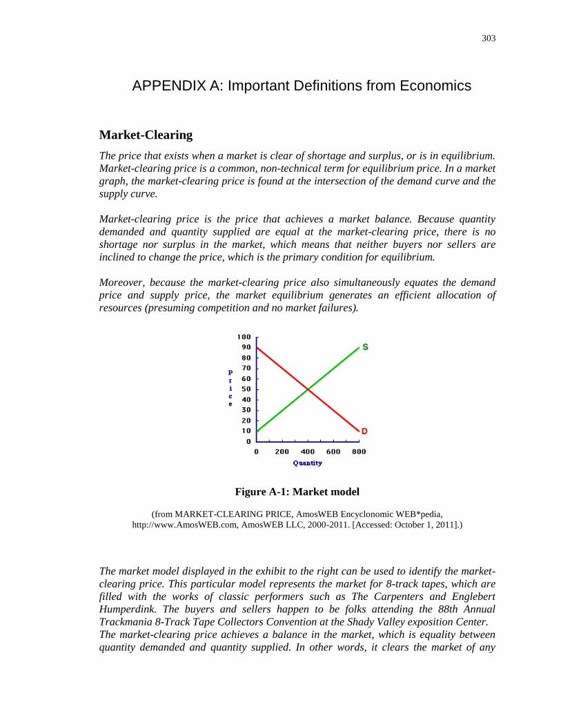
303

APPENDIX A: Important Definitions from Economics

Market-Clearing

The price that exists when a market is clear of shortage and surplus, or is in equilibrium.

Market-clearing price is a common, non-technical term for equilibrium price. In a market

graph, the market-clearing price is found at the intersection of the demand curve and the

supply curve.

Market-clearing price is the price that achieves a market balance. Because quantity

demanded and quantity supplied are equal at the market-clearing price, there is no

shortage nor surplus in the market, which means that neither buyers nor sellers are

inclined to change the price, which is the primary condition for equilibrium.

Moreover, because the market-clearing price also simultaneously equates the demand

price and supply price, the market equilibrium generates an efficient allocation of

resources (presuming competition and no market failures).

Figure A-1: Market model

(from MARKET-CLEARING PRICE, AmosWEB Encyclonomic WEB*pedia,

http://www.AmosWEB.com, AmosWEB LLC, 2000-2011. [Accessed: October 1, 2011].)

The market model displayed in the exhibit to the right can be used to identify the market-

clearing price. This particular model represents the market for 8-track tapes, which are

filled with the works of classic performers such as The Carpenters and Englebert

Humperdink. The buyers and sellers happen to be folks attending the 88th Annual

Trackmania 8-Track Tape Collectors Convention at the Shady Valley exposition Center.

The market-clearing price achieves a balance in the market, which is equality between

quantity demanded and quantity supplied. In other words, it clears the market of any

304

shortage or surplus. The only price that accomplishes this task is at the intersection of the

demand curve and supply curve. This intersection point, and the price that achieves it,

can be identified by clicking the [Market-Clearing Price] button in the exhibit.

Doing so reveals a market-clearing price of 50 cents. At this price, the demand curve and

supply curve intersect. The quantity demanded is 400 tapes and the quantity supplied is

400 tapes. The quantity demanded is equal to the quantity supplied. The buyers can buy

all that they want, so there is no shortage. The sellers can sell all that they want, so there

is no surplus. Neither buyers nor sellers are motivated to change the price. The forces of

demand and supply are in balance.

This is the ONLY price that achieves a balance between these two quantities. Best of all,

because this is equilibrium, the market-clearing price of 50 cents will not change and the

equilibrium quantity of 400 tapes will not change unless or until an external force

intervenes.

Source:

MARKET-CLEARING PRICE, AmosWEB Encyclonomic WEB*pedia,

http://www.AmosWEB.com, AmosWEB LLC, 2000-2011. Last accessed: October 1,

2011.

Neoclassical Growth Model

The neoclassical model of long-run economic growth, introduced by Robert Solow (b.

1924) and Trevor Swan (1918–1989) in 1956, analyzes the convergence of an economy to

a growth rate set by exogenous population increase and, as added the following year by

Solow (1957), an exogenous rate of technical change. Earlier growth models by R. F.

Harrod (1900–1978) in 1939 and Evsey Domar (1914–1997) in 1946 (both reprinted in

Stiglitz and Uzawa 1969) had assumed fixed coefficients in products, which the Solow-

Swan neoclassical model generalized to allow for substitution between capital and labor.

The term neoclassical reflected the model’s concern with long-run equilibrium growth of

potential output in a fully employed economy, abstracting from short-run Keynesian

issues of effective demand.

The neoclassical growth model assumes the existence of an aggregate production

function , where is aggregate output, is the capital stock, and is the

number of workers. The production function has constant returns to scale (if K and N

change in the same proportion, will also change in that proportion), with positive but

diminishing marginal products of capital and labor. Dividing by the number of workers

, output per capita is a function of the capital/labor ratio :

305

and , where is consumption per capita and is investment

per capita. The per capita consumption function is assumed to be — , where

is the marginal propensity to save and — is the marginal propensity to consume. In

equilibrium, (desired) investment is equal to saving, .

Source:

What-when-how, (2011). Neoclassical Growth Model (Social Science). Available at:

http://what-when-how.com/social-sciences/neoclassical-growth-model-social-science/,

last accessed October 1, 2011.

Cobb-Douglas Production Function In economics, the Cobb-Douglas functional form of production functions is widely used

to represent the relationship of an output to inputs. It was proposed by Knut Wicksell

(1851-1926), and tested against statistical evidence by Charles Cobb and Paul Douglas

in 1928.

In 1928 Charles Cobb and Paul Douglas published a study in which they modeled the

growth of the American economy during the period 1899 - 1922. They considered a

simplified view of the economy in which production output is determined by the amount

of labor involved and the amount of capital invested. While there are many other factors

affecting economic performance, their model proved to be remarkably accurate.

The function they used to model production was of the form:

where:

= total production (the monetary value of all goods produced in a year)

= labor input (the total number of person-hours worked in a year)

= capital input (the monetary worth of all machinery, equipment, and buildings)

= total factor productivity

and are the output elasticities of labour and capital, respectively. These values are

constants determined by available technology.

Output elasticity measures the responsiveness of output to a change in levels of either

labour or capital used in production, ceteris paribus. For example if = 0.15, a 1%

increase in labour would lead to approximately a 0.15% increase in output.

Source:

Bao Hong, Tan (2008). Cobb-Douglas Production Function. Available at:

http://docentes.fe.unl.pt/~jamador/Macro/cobb-douglas.pdf, last accessed October 1,

2011.

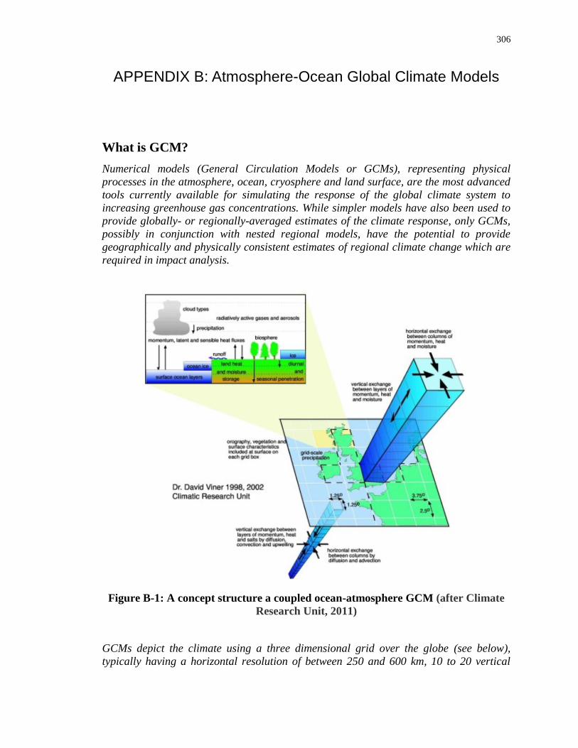
306

APPENDIX B: Atmosphere-Ocean Global Climate Models

What is GCM?

Numerical models (General Circulation Models or GCMs), representing physical

processes in the atmosphere, ocean, cryosphere and land surface, are the most advanced

tools currently available for simulating the response of the global climate system to

increasing greenhouse gas concentrations. While simpler models have also been used to

provide globally- or regionally-averaged estimates of the climate response, only GCMs,

possibly in conjunction with nested regional models, have the potential to provide

geographically and physically consistent estimates of regional climate change which are

required in impact analysis.

Figure B-1: A concept structure a coupled ocean-atmosphere GCM (after Climate

Research Unit, 2011)

GCMs depict the climate using a three dimensional grid over the globe (see below),

typically having a horizontal resolution of between 250 and 600 km, 10 to 20 vertical

307

layers in the atmosphere and sometimes as many as 30 layers in the oceans. Their

resolution is thus quite coarse relative to the scale of exposure units in most impact

assessments. Moreover, many physical processes, such as those related to clouds, also

occur at smaller scales and cannot be properly modelled. Instead, their known properties

must be averaged over the larger scale in a technique known as parameterization. This is

one source of uncertainty in GCM-based simulations of future climate. Others relate to

the simulation of various feedback mechanisms in models concerning, for example, water

vapour and warming, clouds and radiation, ocean circulation and ice and snow albedo.

For this reason, GCMs may simulate quite different responses to the same forcing, simply

because of the way certain processes and feedbacks are modelled.

Sources:

Data Distribution Centre, (May16, 2011). http://www.ipcc-

data.org/ddc_gcm_guide.html, last accesses October 1, 2011

Climate Research Unit, (2011). Available at: http://www.cru.uea.ac.uk/cru/info/modelcc/,

last accessed on October 1, 2011.

CCSM overview

The Community Climate System Model (CCSM) is a coupled climate model for

simulating the earth's climate system. Composed of four separate models simultaneously

simulating the earth's atmosphere, ocean, land surface and sea-ice, and one central

coupler component, the CCSM allows researchers to conduct fundamental research into

the earth's past, present and future climate states.

The CCSM project is a cooperative effort among US climate researchers. Primarily

supported by the National Science Foundation (NSF) and centered at the National Center

for Atmospheric Research (NCAR) in Boulder Colorado, the CCSM project enjoys close

collaborations with the US Department of Energy and the National Air and Space

Administration. Scientific development of the CCSM is guided by the CCSM working

groups, which meet twice a year. More information on the CCSM project, such as the

management structure, the scientific working groups, downloadable source code and

online archives of data from previous CCSM experiments, can be found on the CCSM

website: www.cesm.ucar.edu.

Source:

CCSM3.0 User's Guide, (June 25, 2004). Available at:

http://www.cesm.ucar.edu/models/ccsm3.0/ccsm/doc/UsersGuide/UsersGuide/node3.htm

l, last accesses October 1, 2011

308

CGCM 3.1 The third version of the Canadian Centre for Climate Modelling and Analysis (CCCma)

Coupled Global Climate Model (CGCM3), makes use of the same ocean component as

that used in the earlier The Second Generation Coupled Global Climate Model, but it

makes use of the substantially updated atmospheric component The Third Generation

Atmospheric General Circulation Model. The sea-ice component is a two-category model

(mean thickness and concentration) with cavitating fluid dynamics and thermodynamics

as in The First Generation Coupled Global Climate Model and The Second Generation

Coupled Global Climate Model.

CGCM3.1 is run at two different resolutions. The T47 version has a surface grid whose

spatial resolotion is roughly 3.75 degrees lat/lon and 31 levels in the vertical. The ocean

grid shares the same land mask as the atmsosphere, but has four ocean grid cells

underlying every atmospheric grid cell. The ocean resolution in this case is roughly 1.85

degrees, with 29 levels in the vertical.

The T63 version has a surface grid whose spatial resolution is roughly 2.8 degrees

lat/lon and 31 levels in the vertical. As before the ocean grid shares the same land mask

as the atmosphere, but in this case there are 6 ocean grids underlying every atmospheric

grid cell. The ocean resolution is therefore approximately 1.4 degrees in longitude and

0.94 degrees in latitude. This provides slightly better resolution of zonal currents in the

Tropics, more nearly isotropic resolution at mid latitudes, and somewhat reduced probles

with converging meridians in the Arctic.

Source:

EC, (May 19, 2010). Data: Canadian Centre for Climate Modelling and Analysis,

available at: http://www.cccma.ec.gc.ca/data/cgcm3/cgcm3.shtml, last accessed

October 1, 2011.

CSIRO-MK

Some time ago the Commonwealth Scientific and Industrial Research Organisation

(CSIRO) completed its submission to the IPCC AR4 Model database a set of experiments

simulating past, present and future climate with the Mk3 Climate System. The Mk3 model

has been in development and used for production climate runs for the best part of a

decade and is the end result of a significant commitment of financial and intellectual

resources from a relatively small group of developers and stakeholders.

CSIRO has a long history of being involved in the science of climate and weather and the

CSIRO Mk3 model is the latest in a series of models to be developed for a broad range of

scientific investigations and applications. The CSIRO model is one of about two dozen

recognised climate models operating around the world.

309

Output from two versions of the CSIRO Mk3 model were contributed to the CMIP3 these

are the Mk3.0 and Mk3.5. Briefly, the horizontal resolution of the Mk3.0 atmospheric

model is spectral T63 (approximately 1.875° latitude×1.875° longitude) with 18 vertical

levels (hybrid sigma-pressure vertical coordinate). Readers are further referred to

http://wwwpcmdi.llnl.gov/ipcc/model_documentation/CSIROMk3.0.pdf for a summary of

Mk3.0 model specifications on a standard template for ease of comparison with the other

CMIP3 participating models.

A number of physical parameterisation and numerical improvements were made to the

Mk3.0 model to produce the Mk3.5 version. These include a scheme to control the

strength of the ocean eddy-induced transport, vertical ocean mixing due to wind

generated turbulent kinetic energy, and an improved runoff and river routing method. See

http://wwwpcmdi.llnl.gov/ipcc/model_documentation/CSIROMk3.5.pdf for a summary of

Mk3.5 model specifications.

Source:

Collier, MA, MR Dix, and AC Hirst, (2007). CSIRO Mk3 climate system model and

meeting the strict IPCC AR4 data requirements, MODSIM07 International Congress on

Modelling and Simulation: Land, water & environmental management: integrated

systems for sustainability, Modelling and Simulation Society of Australia and New

Zealand, pp. 582-588. Availavle at:

http://www.mssanz.org.au/MODSIM07/papers/10_s61/CSIROmk3_s61_Collier_.pdf,

last accesses October 1, 2011.

ECHAM5 The 5

th -generation atmospheric general circulation model (ECHAM5) developed at the

Max Planck Institute for Meteorology (MPIM) is the most recent version in a series of

ECHAM models evolving originally from the spectral weather prediction model of the

European Centre for Medium Range Weather Forecasts.

The climate model ECHAM5 has been developed from the ECMWF operational forecast

model cycle 36 (1989) and a comprehensive parameterisation package developed at

Hamburg (therefore the abbreviation HAM). The part describing the dynamics of

ECHAM is based on the ECMWF documentation, which has been modified to describe

the newly implemented features and the changes necessary for climate experiments.

Compared to the previous version, ECHAM4, a number of substantial changes have been

introduced in both the numerics and physics of the model. These include a flux-form

semi-Lagrangian transport scheme for positive definite variables like water components

and chemical tracers, a new longwave radiation scheme, separate prognostic equations

for cloud liquid water and cloud ice, a new cloud microphysical scheme and a

prognostic-statistical cloud cover parameterization. The number of spectral intervals is

increased in both the longwave and shortwave part of the spectrum. Changes have also

been made in the representation of land surface processes, including an implicit coupling

310

between the surface and the atmosphere, and in the representation of orographic drag

forces. Also, a new dataset of land surface parameters has been compiled for the new

model. On the other hand, horizontal and vertical diffusion, cumulus convection and also

the spectral dynamics remain essentially unchanged.

Source:

Roeckner, E., G. Bäuml, L. Bonaventura, R. Brokopf, M. Esch, M. Giorgetta, S.

Hagemann, I. Kirchner, L. Kornblueh, E. Manzini, A. Rhodin, U. Schlese, U.

Schulzweida, A. Tompkins, (2003). The atmospheric general circulation model

ECHAM5: Model description, Report No. 349, Max Planck Institute for Meteorology,

Hamburg, 140 pages. Available at :

http://www.mpimet.mpg.de/fileadmin/publikationen/Reports/max_scirep_349.pdf, last

accessed October 1, 2011.

ECHO-G

ECHO-G is a global coupled atmosphere-ocean climate model whose component models

are the ECHAM atmosphere general circulation model and a global version of the

Hamburg Ocean Primitive Equation model, HOPE-G, which includes a dynamic-

thermodynamic sea-ice model with snow cover. ECHO-G can be used in numerical

studies of natural variability of the world climate and of climate changes on time-scales

ranging from the component models time steps to centuries. In high latitudes, the

interaction between ocean and atmosphere can be strongly affected by the sea-ice cover.

In particular, the heat flux through ice and that through leads and polynyas can differ by

an order of magnitude on horizontal scales much smaller than that of a grid-cell in

global climate models. ECHOG accounts for these effects by a separate calculation of

fluxes over ice and over water when a sub-grid-scale partial ice cover is present.

Source:

Modellberatungsgruppe, DKRZ, (1999). The Hamburg Atmosphere-Ocean Coupled

Circulation Model E C H O-G, Technical Report No. 18, Hamburg, 74 pages. Available

at: http://www.mad.zmaw.de/fileadmin/extern/documents/reports/ReportNo.18.pdf, last

accessed October 1, 2011.

GFDL CM2.0

In 2004, a new family of global coupled AOGCMs (the CM2.x family) was first used to

conduct climate research studies at NOAA’s Geophysical Fluid Dynamics Laboratory

(GFDL). The GFDL CM2.0 & CM2.1 models represent a clean break from previous

generations of GFDL climate models. All of the coupled model components (the

atmosphere, ocean, sea ice, and land surface models) were developed from new codes.

In both CM2.0 and CM2.1, the atmospheric model’s horizontal grid dimensions are 144

by 90 (about 2.5° longitude by 2.0

° latitude spacing). However, the exact horizontal grid

311

locations are not the same in the two models. Both have 24 vertical levels and use a

hybrid coordinate grid, in which sigma surfaces near the ground continuously transform

to pressure surfaces above 250 hP. The lowest model level is about 30m above the

surface. Two sets of 10 IPCC AR4 related simulations have been run; one using the

GFDL CM2.0 model and one using the GFDL CM2.1 model. Processed model output

files from the GFDL CM2.x simulations are available to researchers via both the

PCMDI/IPCC WGI Archive & the GFDL Data Portal.

Source:

Geographysical fluid dynamics laboratory, (June 10, 2010). GFDL CM2.X coupled

climate models, available at: http://nomads.gfdl.noaa.gov/CM2.X/CM2xHI.pdf, last

accessed October 1, 2011.

GISS

The global coupled Atmosphere-Ocean Model was designed at GISS for climate

predictions at decade to century time scales. Atmospheric Models at GISS have been

under continual development since 1970; the Ocean and Coupled Models since 1990.

The Atmosphere-Ocean Model is a computer program that simulates the Earth's climate

in three dimensions on a gridded domain. The Model requires two kinds of input,

specified parameters and prognostic variables, and generates two kinds of output,

climate diagnostics and prognostic variables. The specified input parameters include

physical constants, the Earth's orbital parameters, the Earth's atmospheric constituents,

the Earth's topography, the Earth's surface distribution of ocean, glacial ice, or

vegetation, and many others. The time varying prognostic variables include fluid mass,

horizontal velocity, heat, water vapor, salt, and subsurface mass and energy fields.

For the 1999 version of the Atmosphere-Ocean Model, six 150-year simulations were

run: C089 and C092 are control simulations with constant 1950 atmospheric

composition; C090 and C093 use observed greenhouse gases from 1950 to 1990 and

compounded annual .5% CO2 increases from 1991 to 2099; C091 and C094 use the

varying greenhouse gases plus tropospheric sulfate aerosol changes. Annual .5% CO2

increases after 1990 were chosen because they match the current radiative forcing

caused by all greenhouse gases.

Source:

Russell, Gary L., (February 2, 2011). General Information about 5x4 Atmosphere-Ocean

Model, available at: http://aom.giss.nasa.gov/general.html, last accessed October 2, 2011.

IPSL CM4

The IPSL CM4 model couples four components of the Earth system: LMDZ for

atmospheric dynamics and physics, OPA for ocean dynamics, LIM for sea ice dynamics

312

and thermodynamics, and ORCHIDEE for the land surface. Successive versions of the

global coupled model have been developed since 1995. Since the first version of the

coupled model, the goal was to design and develop a global coupled model with no flux

correction at the air–sea interface that can be used to study present, future and past

climates. Substantial development and analysis concerned the conservation of energy and

water, so that comprehensive analyses of heat and water budget and transport are

possible.

The first version of the model was built with the LMD 5.3 version of the LMD

atmospheric model, the OPA 7 version of the ocean model developed at LODYC, and a

simple sea ice component. The first coupled simulations exhibited a large drift in surface

air temperature, which has been attributed to an energetic imbalance of the atmospheric

model. Several adjustments were performed.

The next step of the model development consisted in implementing the complex IPSL

thermodynamic sea ice model. It was also coupled to a carbon cycle model, to perform

the first climate simulations (present and future) with an interactive carbon cycle.

The latest developments lead to a completely new model used for CMIP3, the multimodel

ensembles climate projections used in the intergovernmental panel on climate change

(IPCC) assessment report AR4 (IPCC 2007). The model climatology and the

representation of the interannual variability were greatly improved compared to the

previous generations, even though some biases are still present.

Source:

Marti, Olivier, P. Braconnot, J.-L. Dufresne, J. Bellier, R. Benshila, S. Bony, P.

Brockmann, P. Cadule, A. Caubel, F. Codron, N. de Noblet, S. Denvil, L. Fairhead, T.

Fichefet, M.-A. Foujols, P. Friedlingstein, H. Goosse, J.-Y. Grandpeix, E. Guilyardi, F.

Hourdin, A. Idelkadi, M. Kageyama, G. Krinner, C. Le´vy, G. Madec, J. Mignot, I.

Musat, D. Swingedouw, C. Talandier, (2010). Key features of the IPSL ocean atmosphere

model and its sensitivity to atmospheric resolution. CLIMATE DYNAMICS, 34(1): 1-

26, DOI: 10.1007/s00382-009-0640-6

MRI-CGCM

A new version of a global coupled atmosphere-ocean general circulation model (MRI-

CGCM2) has been developed at the Meteorological Research Institute (MRI). The model

can be used to explore climate change associated with anthropogenic forcings. It aimed

to reduce the drawbacks of the former version of the model (MRI-CGCM1) and achieve a

more realistic climatic mean and variability to predict climate changes with greater

accuracy.

In a preliminary analysis of the control run, the model showed generally good

performance in reproducing the mean climate (including seasonal variation) in

representative aspects; surface air temperature, precipitation, snow and sea ice

313

distribution, and ocean structure and circulation. The model is capable of making a

stable integration longer than 200 years.

Source:

Seiji Yukimoto, Akira Noda, Akio Kitoh, Masato Sugi, Yoshiteru Kitamura, Masahiro

Hosaka, Kiyotaka Shibata, Shuhei Maeda and Takao Uchiyama, (2000). The New

Meteorological Research Institute Coupled GCM (MRI-CGCM2)

Model Climate and Variability, Papers in Meteorology and Geophysics, 51(2): 47-88.

PCM

This is a joint effort to develop a DOE-sponsored parallel climate model between Los

Alamos National Laboratory (LANL), the Naval Postgraduate School (NPG), the US

Army Corps of Engineers' Cold Regions Research and Engineering Lab (CRREL) and the

National Center for Atmospheric Research (NCAR). It is coupled with the NCAR

Community Climate Model version 3, the LANL Parallel Ocean Program, and a sea ice

model from the Naval Postgraduate School together in a massively parallel computer

environment. This is Version 1 of the PCM (PCM1).

The atmospheric component is the massively parallel version of the NCAR Community

Climate Model version 3.2 (CCM3). This model includes the latest versions of radiation,

boundary physics, and precipitation physics and is a state-of-the-art atmospheric

component. The CCM3 also includes the land surface model (LSM) which takes into

account soil physics and vegetation.

The grid is 384 x 288 x 32, with an average resolution of 2/3 degree latitude and

longitude with increased latitudinal resolution near the equator of approximately 1/2

degree. This model is being spun up with observed surface and subsurface forcing in

preparation for coupling. The model in its present form yields an extraordinary

simulation of the Arctic Ocean, tropical Pacific, and boundary currents, such as the Gulf

Stream, with eddies solved in most basins. The PCTM ice model contains the same

physics as the 2001 version of the NCAR CCSM sea ice component, although the two

models have different adaptations for time-sequence in coupling to the other components

and for separate execution on parallel processors.

Source:

Parallet Climate Model, (August 26, 2004). Available at: http://www.cgd.ucar.edu/pcm/, last

accessed October 2, 2011.

HadCM3 HadCM3 (abbreviation for Hadley Centre Coupled Model, version 3) is a coupled

atmosphere-ocean general circulation model (AOGCM) developed at the Hadley Centre

314

in the United Kingdom. It was one of the major models used in the IPCC Third

Assessment Report in 2001. Unlike earlier AOGCMs at the Hadley Centre and elsewhere

(including its predecessor HadCM2), HadCM3 does not need flux adjustment (additional

"artificial" heat and freshwater fluxes at the ocean surface) to produce a good

simulation. The higher ocean resolution of HadCM3 is a major factor in this; other

factors include a good match between the atmospheric and oceanic components; and an

improved ocean mixing scheme (Gent and McWilliams). HadCM3 has been run to

produce simulations for periods of over a thousand years, showing little drift in its

surface climate. HadCM3 is composed of two components: the atmospheric model

HadAM3 and the ocean model (which includes a sea ice model). Simulations often use a

360-day calendar, where each month is 30 days. For more details see,

http://en.wikipedia.org/wiki/HadCM3.

Source:

UNIL (2011). Geocatalogue, available at:

http://www2.unil.ch/sig/geocatalog/gc_results.php?Sources%5B%5D=worldclim,future,h

adcm3 , last accessed October 02, 2011

HadGEM1

A new coupled general circulation climate model developed at the Met Office’s Hadley

Centre is presented, and aspects of its performance in climate simulations run for the

Intergovernmental Panel on Climate Change Fourth Assessment Report (IPCC AR4)

documented with reference to previous models. The Hadley Centre Global Environmental

Model version 1 (HadGEM1) is built around a new atmospheric dynamical core; uses

higher resolution than the previous Hadley Centre model, HadCM3; and contains several

improvements in its formulation including interactive atmospheric aerosols (sulphate,

black carbon, biomass burning, and sea salt) plus their direct and indirect effects. The

ocean component also has higher resolution and incorporates a sea ice component more

advanced than HadCM3 in terms of both dynamics and thermodynamics. The simulation

of present-day mean climate in HadGEM1 is significantly better overall in comparison to

HadCM3, although some deficiencies exist in the simulation of tropical climate and El

Niño variability. HadGEM1 is anticipated to be used as the basis both for higher-

resolution and higher-complexity Earth System studies in the near future.

Source:

T. C. Johns, C. F. Durman, H. T. Banks, M. J. Roberts, A. J. McLaren, J. K. Ridley, C. A.

Senior, K. D. Williams, A. Jones, G. J. Rickard, S. Cusack, W. J. Ingram, M. Crucifix, D.

M. H. Sexton, M. M. Joshi, B-W. Dong, H. Spencer, R. S. R. Hill, J. M. Gregory, A.B.

Keen, A. K. Pardaens, J. A. Lowe, A. Bodas-Salcedo, S. Stark, and Y. Searl, (2006). The

new Hadley Centre climate model HadGEM1: Evaluation of coupled simulations, J.

Climate, 19(7): 1327- 353.

315

APPENDIX C: Data Processing of GCM’s

Architecture of the system

Figure C-1: Architecture of the data processing system

Sample report:

Figure C-2: Snapshot of the parameter input window

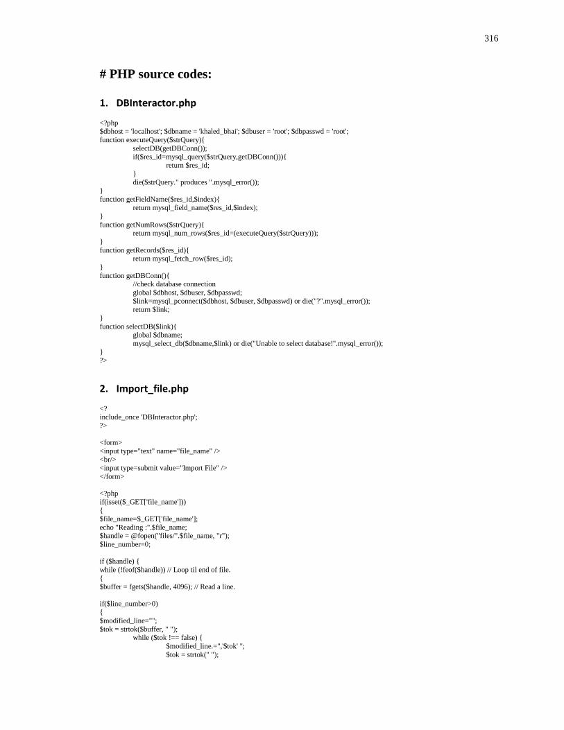
316

# PHP source codes:

1. DBInteractor.php

<?php $dbhost = 'localhost'; $dbname = 'khaled_bhai'; $dbuser = 'root'; $dbpasswd = 'root';

function executeQuery($strQuery){

selectDB(getDBConn()); if($res_id=mysql_query($strQuery,getDBConn())){

return $res_id;

} die($strQuery." produces ".mysql_error());

}

function getFieldName($res_id,$index){ return mysql_field_name($res_id,$index);

}

function getNumRows($strQuery){ return mysql_num_rows($res_id=(executeQuery($strQuery)));

}

function getRecords($res_id){ return mysql_fetch_row($res_id);

}

function getDBConn(){ //check database connection

global $dbhost, $dbuser, $dbpasswd;

$link=mysql_pconnect($dbhost, $dbuser, $dbpasswd) or die("?".mysql_error()); return $link;

}

function selectDB($link){ global $dbname;

mysql_select_db($dbname,$link) or die("Unable to select database!".mysql_error());

} ?>

2. Import_file.php

<? include_once 'DBInteractor.php';

?>

<form>

<input type="text" name="file_name" />

<br/> <input type=submit value="Import File" />

</form>

<?php

if(isset($_GET['file_name']))

{ $file_name=$_GET['file_name'];

echo "Reading :".$file_name; $handle = @fopen("files/".$file_name, "r");

$line_number=0;

if ($handle) {

while (!feof($handle)) // Loop til end of file.

{ $buffer = fgets($handle, 4096); // Read a line.

if($line_number>0) {

$modified_line="";

$tok = strtok($buffer, " "); while ($tok !== false) {

$modified_line.=",'$tok' ";

$tok = strtok(" ");

317

}

$modified_line=substr($modified_line,1,1000); $query="insert into monthly_data values ($modified_line);";

executeQuery($query);

} $line_number++;

}

fclose($handle); // Close the file. }

executeQuery("commit;");

echo $line_number." lines imported."; }

?>

3. Report.php

<?

include_once("DBInteractor.php");

if(getData('select count(*) from monthly_data where data_month in

("JAN","FEB","MAR","APR","MAY","JUN","JUL","AUG","SEP","OCT","NOV","DEC");')!=0) {

executeQuery('update monthly_data set data_month=1 WHERE data_month like "%JAN%"');

executeQuery('update monthly_data set data_month=2 WHERE data_month like "%FEB%"'); executeQuery('update monthly_data set data_month=3 WHERE data_month like "%MAR%"');

executeQuery('update monthly_data set data_month=4 WHERE data_month like "%APR%"');

executeQuery('update monthly_data set data_month=5 WHERE data_month like "%MAY%"'); executeQuery('update monthly_data set data_month=6 WHERE data_month like "%JUN%"');

executeQuery('update monthly_data set data_month=7 WHERE data_month like "%JUL%"');

executeQuery('update monthly_data set data_month=8 WHERE data_month like "%AUG%"'); executeQuery('update monthly_data set data_month=9 WHERE data_month like "%SEP%"');

executeQuery('update monthly_data set data_month=10 WHERE data_month like "%OCT%"');

executeQuery('update monthly_data set data_month=11 WHERE data_month like "%NOV%"'); executeQuery('update monthly_data set data_month=12 WHERE data_month like "%DEC%"');

}

?>

<table>

<form> <tr>

<td>

Start Year</td> <td>

<select name="startyear" id="startyear">

<? for($i=1901;$i<2000;$i++)

echo("<option value=".($i-1900)." > $i </option>");

?>

</select>

</td></tr> <tr>

<td>

Start Month </td>

<td>

<select name="startmonth" id="startmonth"> <option value='1'>JAN</option>

<option value='2'>FEB</option>

<option value='3'>MAR</option> <option value='4'>APR</option>

<option value='5'>MAY</option>

<option value='6'>JUN</option> <option value='7'>JUL</option>

<option value='8'>AUG</option>

<option value='9'>SEP</option> <option value='10'>OCT</option>

<option value='11'>NOV</option>

318

<option value='12'>DEC</option>

</select> </td>

</tr>

<tr> <td>

End Year</td>

<td> <select name="endyear" id="endyear">

<?

for($i=1901;$i<2000;$i++) echo("<option value=".($i-1900)." > $i </option>");

?>

</select>

</td>

</tr> <tr>

<td>

End Month

</td>

<td>

<select name="endmonth" id="endmonth"> <option value='1'>JAN</option>

<option value='2'>FEB</option>

<option value='3'>MAR</option> <option value='4'>APR</option>

<option value='5'>MAY</option> <option value='6'>JUN</option>

<option value='7'>JUL</option>

<option value='8'>AUG</option> <option value='9'>SEP</option>

<option value='10'>OCT</option>

<option value='11'>NOV</option> <option value='12'>DEC</option>

</select>

</td>

</tr>

<tr> <td>

X1

</td><td> <input type="text" name=x1 />

</td>

</tr> <tr>

<td>

X2 </td><td>

<input type="text" name=x2 />

</td> </tr>

<tr>

<td> Y1

</td><td>

<input type="text" name=y1 />

</td>

</tr>

<tr> <td>

Y2

</td><td> <input type="text" name=y2 />

</td>

</tr> <tr>

<td>

Report

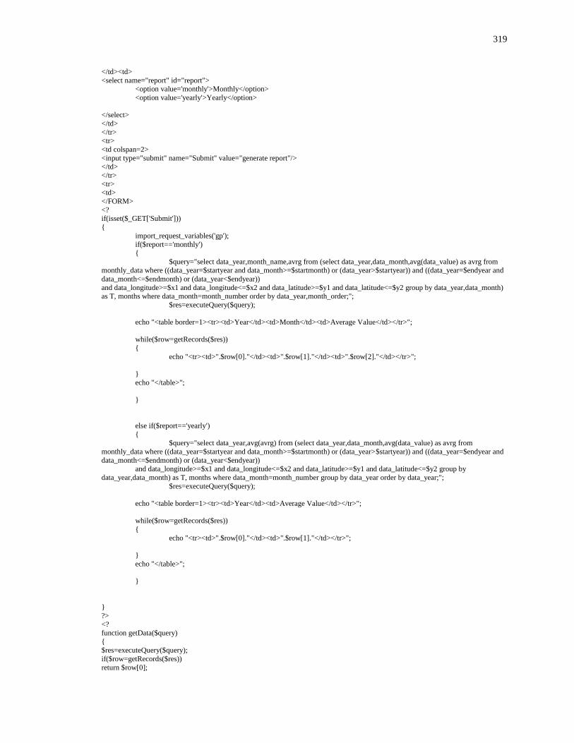
319

</td><td>

<select name="report" id="report"> <option value='monthly'>Monthly</option>

<option value='yearly'>Yearly</option>

</select>

</td>

</tr> <tr>

<td colspan=2>

<input type="submit" name="Submit" value="generate report"/> </td>

</tr>

<tr> <td>

</FORM>

<? if(isset($_GET['Submit']))

{

import_request_variables('gp');

if($report=='monthly')

{

$query="select data_year,month_name,avrg from (select data_year,data_month,avg(data_value) as avrg from monthly_data where ((data_year=$startyear and data_month>=$startmonth) or (data_year>$startyear)) and ((data_year=$endyear and

data_month<=$endmonth) or (data_year<$endyear))

and data_longitude>=$x1 and data_longitude<=$x2 and data_latitude>=$y1 and data_latitude<=$y2 group by data_year,data_month) as T, months where data_month=month_number order by data_year,month_order;";

$res=executeQuery($query);

echo "<table border=1><tr><td>Year</td><td>Month</td><td>Average Value</td></tr>";

while($row=getRecords($res))

{

echo "<tr><td>".$row[0]."</td><td>".$row[1]."</td><td>".$row[2]."</td></tr>";

}

echo "</table>";

}

else if($report=='yearly')

{ $query="select data_year,avg(avrg) from (select data_year,data_month,avg(data_value) as avrg from

monthly_data where ((data_year=$startyear and data_month>=$startmonth) or (data_year>$startyear)) and ((data_year=$endyear and

data_month<=$endmonth) or (data_year<$endyear)) and data_longitude>=$x1 and data_longitude<=$x2 and data_latitude>=$y1 and data_latitude<=$y2 group by

data_year,data_month) as T, months where data_month=month_number group by data_year order by data_year;";

$res=executeQuery($query);

echo "<table border=1><tr><td>Year</td><td>Average Value</td></tr>";

while($row=getRecords($res))

{

echo "<tr><td>".$row[0]."</td><td>".$row[1]."</td></tr>";

}

echo "</table>";

}

}

?> <?

function getData($query)

{ $res=executeQuery($query);

if($row=getRecords($res))

return $row[0];

320

return 0; }

?>

4. Report2.php

<? include_once("DBInteractor.php");

if(getData('select count(*) from monthly_data where data_value like "%Request%";')!=0)

executeQuery('delete from monthly_data where data_value like "%Request%";');

if(getData('select count(*) from monthly_data where data_month in

("JAN","FEB","MAR","APR","MAY","JUN","JUL","AUG","SEP","OCT","NOV","DEC");')!=0) {

executeQuery('update monthly_data set data_month=1 WHERE data_month like "%JAN%"');

executeQuery('update monthly_data set data_month=2 WHERE data_month like "%FEB%"'); executeQuery('update monthly_data set data_month=3 WHERE data_month like "%MAR%"');

executeQuery('update monthly_data set data_month=4 WHERE data_month like "%APR%"');

executeQuery('update monthly_data set data_month=5 WHERE data_month like "%MAY%"'); executeQuery('update monthly_data set data_month=6 WHERE data_month like "%JUN%"');

executeQuery('update monthly_data set data_month=7 WHERE data_month like "%JUL%"');

executeQuery('update monthly_data set data_month=8 WHERE data_month like "%AUG%"'); executeQuery('update monthly_data set data_month=9 WHERE data_month like "%SEP%"');

executeQuery('update monthly_data set data_month=10 WHERE data_month like "%OCT%"');

executeQuery('update monthly_data set data_month=11 WHERE data_month like "%NOV%"'); executeQuery('update monthly_data set data_month=12 WHERE data_month like "%DEC%"');

}

$sql="select * from (

select data_day,data_month,data_year,data_latitude,data_longitude,data_value, count(*) as counts from monthly_data group by data_day,data_month,data_year,data_latitude,data_longitude) as T where counts>1";

$res=executeQuery($sql);

while($rw=getRecords($res)) {

$data_day=$rw[0];

$data_month=$rw[1];

$data_year=$rw[2];

$data_latitude=$rw[3]; $data_longitude=$rw[4];

$data_value=$rw[5];

executeQuery("delete from monthly_data where data_day='$data_day' and data_month='$data_month' and data_year='$data_year' and

data_latitude='$data_latitude' and data_longitude='$data_longitude' ");

executeQuery("insert into monthly_data (data_day,data_month,data_year,data_latitude,data_longitude,data_value) values

('$data_day','$data_month','$data_year','$data_latitude','$data_longitude','$data_value')");

}

?>

<table border=0> <form>

<tr>

<td> Start Year</td>

<td>

<select name="startyear" id="startyear"> <?

for($i=1901;$i<2000;$i++)

echo("<option value=".($i-1900)." > $i </option>"); ?>

</select> </td></tr>

<tr>

321

<td>

Start Month </td>

<td>

<select name="startmonth" id="startmonth"> <option value='1'>JAN</option>

<option value='2'>FEB</option>

<option value='3'>MAR</option> <option value='4'>APR</option>

<option value='5'>MAY</option>

<option value='6'>JUN</option> <option value='7'>JUL</option>

<option value='8'>AUG</option>

<option value='9'>SEP</option> <option value='10'>OCT</option>

<option value='11'>NOV</option>

<option value='12'>DEC</option> </select>

</td>

</tr>

<tr>

<td>

End Year</td> <td>

<select name="endyear" id="endyear">

<? for($i=1901;$i<2000;$i++)

echo("<option value=".($i-1900)." > $i </option>"); ?>

</select> </td>

</tr>

<tr>

<td>

End Month </td>

<td>

<select name="endmonth" id="endmonth">

<option value='1'>JAN</option> <option value='2'>FEB</option>

<option value='3'>MAR</option>

<option value='4'>APR</option> <option value='5'>MAY</option>

<option value='6'>JUN</option>

<option value='7'>JUL</option> <option value='8'>AUG</option>

<option value='9'>SEP</option>

<option value='10'>OCT</option> <option value='11'>NOV</option>

<option value='12'>DEC</option>

</select>

</td>

</tr>

<tr>

<td>

longitude start

</td><td> <input type="text" name=x1 value="-180" />

</td> </tr>

<tr>

<td>

322

longitude end

</td><td> <input type="text" name=x2 value="180" />

</td> </tr>

<tr>

<td> longitude interval

</td><td>

<input type="text" name=xinterval /> </td>

</tr>

<tr> <td>

latitude start

</td><td> <input type="text" name=y1 value="-90" />

</td>

</tr>

<tr>

<td>

latitude end </td><td>

<input type="text" name=y2 value="90" />

</td> </tr>

<tr>

<td>

latitude interval </td><td>

<input type="text" name=yinterval />

</td> </tr>

<tr>

<td> Report

</td><td>

<select name="report" id="report"> <option value='monthly'>Monthly</option>

<option value='yearly'>Yearly</option>

</select> </td>

</tr>

<tr> <td colspan=2>

<input type="submit" name="Submit" value="generate report"/>

</td> </tr>

</FORM>

</table>

<br/>

<br/>

<?

if(isset($_GET['Submit']))

{

import_request_variables('gp');

if($report=='monthly') {

$data="";

for($xstart=$x1; $xstart<$x2; $xstart=$xstart+$xinterval)

{ $xend=$xstart+$xinterval;

for($ystart=$y1; $ystart<$y2; $ystart=$ystart+$yinterval)

323

{

$yend=$ystart+$yinterval;

$query="select data_year,month_name,avrg from (select data_year,data_month,avg(data_value) as avrg from monthly_data where ((data_year=$startyear and data_month>=$startmonth) or (data_year>$startyear)) and ((data_year=$endyear and

data_month<=$endmonth) or (data_year<$endyear))

and data_longitude>=$xstart and data_longitude<=$xend and data_latitude>=$ystart and data_latitude<=$yend group by data_year,data_month) as T, months where data_month=month_number order by data_year,month_order;";

$res=executeQuery($query);

$xav=($xstart+$xend)/2;

$yav=($ystart+$yend)/2;

while($row=getRecords($res))

{ $data[$row[0]][$row[1]][$xav][$yav]=$row[2];

}

}

} $query="select data_year,month_name,avrg from (select data_year,data_month,avg(data_value) as avrg from

monthly_data where ((data_year=$startyear and data_month>=$startmonth) or (data_year>$startyear)) and ((data_year=$endyear and

data_month<=$endmonth) or (data_year<$endyear)) and data_longitude>=$x1 and data_longitude<=$x2 and data_latitude>=$y1 and data_latitude<=$y2 group by data_year,data_month)

as T, months where data_month=month_number order by data_year,month_order;"; $res=executeQuery($query);

echo "<table border=1><tr><td>Year</td><td>Month</td>";

for($xstart=$x1; $xstart<$x2; $xstart=$xstart+$xinterval) {

$xend=$xstart+$xinterval;

for($ystart=$y1; $ystart<$y2; $ystart=$ystart+$yinterval) {

$yend=$ystart+$yinterval;

$xav=($xstart+$xend)/2;

$yav=($ystart+$yend)/2;

echo "<td>".$xav.",".$yav."</td>"; }

}

echo "<td>Average Value</td></tr>";

$query="select data_year,month_name,avrg from (select data_year,data_month,avg(data_value) as avrg from

monthly_data where ((data_year=$startyear and data_month>=$startmonth) or (data_year>$startyear)) and ((data_year=$endyear and data_month<=$endmonth) or (data_year<$endyear))

and data_longitude>=$x1 and data_longitude<=$x2 and data_latitude>=$y1 and data_latitude<=$y2 group by data_year,data_month)

as T, months where data_month=month_number order by data_year,month_order;"; $res=executeQuery($query);

while($row=getRecords($res)) {

echo "<tr><td>".$row[0]."</td><td>".$row[1]."</td>";

for($xstart=$x1; $xstart<$x2; $xstart=$xstart+$xinterval) {

$xend=$xstart+$xinterval;

for($ystart=$y1; $ystart<$y2; $ystart=$ystart+$yinterval)

{

$yend=$ystart+$yinterval;

$xav=($xstart+$xend)/2; $yav=($ystart+$yend)/2;

if($data[$row[0]][$row[1]][$xav][$yav]=="") echo "<td>0</td>";

else

echo "<td>".$data[$row[0]][$row[1]][$xav][$yav]."</td>";

324

}

} echo "<td>".$row[2]."</td></tr>";

}

echo "</table>"; }

else if($report=='yearly') {

$data=""; for($xstart=$x1; $xstart<$x2; $xstart=$xstart+$xinterval)

{

$xend=$xstart+$xinterval;

for($ystart=$y1; $ystart<$y2; $ystart=$ystart+$yinterval)

{

$yend=$ystart+$yinterval;

$query="select data_year,avg(avrg) from (select data_year,data_month,avg(data_value) as avrg from

monthly_data where ((data_year=$startyear and data_month>=$startmonth) or (data_year>$startyear)) and ((data_year=$endyear and

data_month<=$endmonth) or (data_year<$endyear)) and data_longitude>=$xstart and data_longitude<=$xend and data_latitude>=$ystart and data_latitude<=$yend group by

data_year,data_month) as T, months where data_month=month_number group by data_year order by data_year;";

$res=executeQuery($query);

$xav=($xstart+$xend)/2; $yav=($ystart+$yend)/2;

while($row=getRecords($res)) {

$data[$row[0]][$xav][$yav]=$row[1];

}

}

}

$query="select data_year,avg(avrg) from (select data_year,data_month,avg(data_value) as avrg from

monthly_data where ((data_year=$startyear and data_month>=$startmonth) or (data_year>$startyear)) and ((data_year=$endyear and

data_month<=$endmonth) or (data_year<$endyear)) and data_longitude>=$x1 and data_longitude<=$x2 and data_latitude>=$y1 and data_latitude<=$y2 group by

data_year,data_month) as T, months where data_month=month_number group by data_year order by data_year;";

$res=executeQuery($query);

echo "<table border=1><tr><td>Year</td>";

for($xstart=$x1; $xstart<$x2; $xstart=$xstart+$xinterval)

{ $xend=$xstart+$xinterval;

for($ystart=$y1; $ystart<$y2; $ystart=$ystart+$yinterval) {

$yend=$ystart+$yinterval;

$xav=($xstart+$xend)/2;

$yav=($ystart+$yend)/2;

echo "<td>".$xav.",".$yav."</td>"; }

}

echo "<td>Average Value</td></tr>";

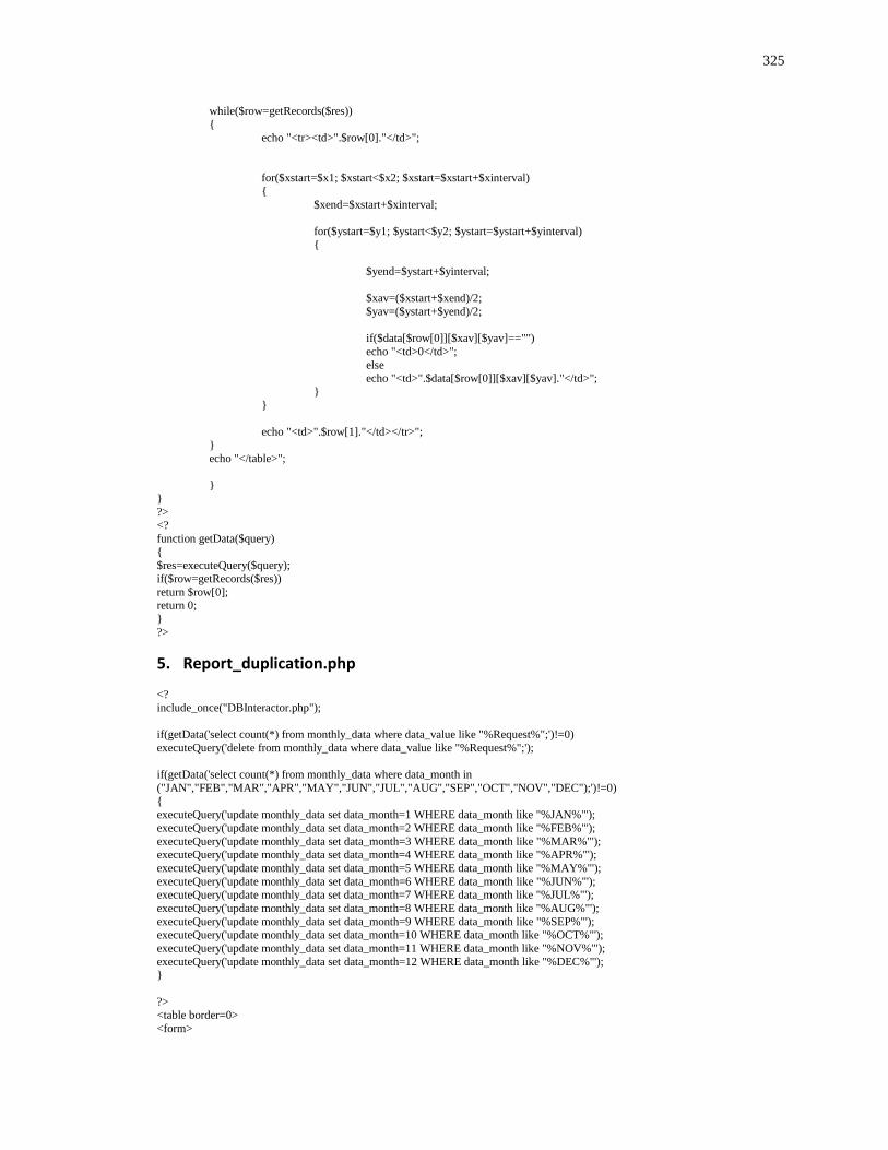
325

while($row=getRecords($res))

{ echo "<tr><td>".$row[0]."</td>";

for($xstart=$x1; $xstart<$x2; $xstart=$xstart+$xinterval)

{

$xend=$xstart+$xinterval;

for($ystart=$y1; $ystart<$y2; $ystart=$ystart+$yinterval)

{

$yend=$ystart+$yinterval;

$xav=($xstart+$xend)/2;

$yav=($ystart+$yend)/2;

if($data[$row[0]][$xav][$yav]=="")

echo "<td>0</td>";

else

echo "<td>".$data[$row[0]][$xav][$yav]."</td>";

}

}

echo "<td>".$row[1]."</td></tr>";

} echo "</table>";

}

}

?> <?

function getData($query)

{ $res=executeQuery($query);

if($row=getRecords($res))

return $row[0]; return 0;

}

?>

5. Report_duplication.php

<? include_once("DBInteractor.php");

if(getData('select count(*) from monthly_data where data_value like "%Request%";')!=0)

executeQuery('delete from monthly_data where data_value like "%Request%";');

if(getData('select count(*) from monthly_data where data_month in

("JAN","FEB","MAR","APR","MAY","JUN","JUL","AUG","SEP","OCT","NOV","DEC");')!=0)

{ executeQuery('update monthly_data set data_month=1 WHERE data_month like "%JAN%"');

executeQuery('update monthly_data set data_month=2 WHERE data_month like "%FEB%"');

executeQuery('update monthly_data set data_month=3 WHERE data_month like "%MAR%"'); executeQuery('update monthly_data set data_month=4 WHERE data_month like "%APR%"');

executeQuery('update monthly_data set data_month=5 WHERE data_month like "%MAY%"');

executeQuery('update monthly_data set data_month=6 WHERE data_month like "%JUN%"'); executeQuery('update monthly_data set data_month=7 WHERE data_month like "%JUL%"');

executeQuery('update monthly_data set data_month=8 WHERE data_month like "%AUG%"');

executeQuery('update monthly_data set data_month=9 WHERE data_month like "%SEP%"'); executeQuery('update monthly_data set data_month=10 WHERE data_month like "%OCT%"');

executeQuery('update monthly_data set data_month=11 WHERE data_month like "%NOV%"');

executeQuery('update monthly_data set data_month=12 WHERE data_month like "%DEC%"'); }

?> <table border=0>

<form>

326

<tr>

<td> Start Year</td>

<td>

<select name="startyear" id="startyear"> <?

for($i=1901;$i<2000;$i++)

echo("<option value=".($i-1900)." > $i </option>"); ?>

</select>

</td></tr> <tr>

<td>

Start Month </td>

<td>

<select name="startmonth" id="startmonth"> <option value='1'>JAN</option>

<option value='2'>FEB</option>

<option value='3'>MAR</option>

<option value='4'>APR</option>

<option value='5'>MAY</option>

<option value='6'>JUN</option> <option value='7'>JUL</option>

<option value='8'>AUG</option>

<option value='9'>SEP</option> <option value='10'>OCT</option>

<option value='11'>NOV</option> <option value='12'>DEC</option>

</select>

</td> </tr>

<tr>

<td> End Year</td>

<td>

<select name="endyear" id="endyear"> <?

for($i=1901;$i<2000;$i++)

echo("<option value=".($i-1900)." > $i </option>"); ?>

</select> </td>

</tr>

<tr>

<td>

End Month </td>

<td> <select name="endmonth" id="endmonth">

<option value='1'>JAN</option>

<option value='2'>FEB</option> <option value='3'>MAR</option>

<option value='4'>APR</option>

<option value='5'>MAY</option>

<option value='6'>JUN</option>

<option value='7'>JUL</option>

<option value='8'>AUG</option> <option value='9'>SEP</option>

<option value='10'>OCT</option>

<option value='11'>NOV</option> <option value='12'>DEC</option>

</select>

</td>

</tr>

<tr>

327

<td>

longitude start

</td><td> <input type="text" name=x1 value="-180" />

</td> </tr>

<tr>

<td> longitude end

</td><td>

<input type="text" name=x2 value="180" />

</td>

</tr>

<tr>

<td>

longitude interval

</td><td> <input type="text" name=xinterval />

</td> </tr>

<tr>

<td>

latitude start </td><td>

<input type="text" name=y1 value="-90" />

</td> </tr>

<tr>

<td> latitude end

</td><td>

<input type="text" name=y2 value="90" /> </td>

</tr>

<tr>

<td>

latitude interval </td><td>

<input type="text" name=yinterval />

</td>

</tr>

<tr>

<td>

Report </td><td>

<select name="report" id="report">

<option value='monthly'>Monthly</option>

<option value='yearly'>Yearly</option>

</select> </td>

</tr>

<tr> <td colspan=2>

<input type="submit" name="Submit" value="generate report"/>

</td> </tr>

</FORM>

328

</table>

<br/> <br/>

<?

if(isset($_GET['Submit']))

{ import_request_variables('gp');

if($report=='monthly')

{

$data="";

for($xstart=$x1; $xstart<$x2; $xstart=$xstart+$xinterval)

{

$xend=$xstart+$xinterval;

for($ystart=$y1; $ystart<$y2; $ystart=$ystart+$yinterval)

{

$yend=$ystart+$yinterval;

$query="select data_year,month_name,avrg from (select data_year,data_month,avg(data_value) as avrg from

monthly_data where ((data_year=$startyear and data_month>=$startmonth) or (data_year>$startyear)) and ((data_year=$endyear and

data_month<=$endmonth) or (data_year<$endyear)) and data_longitude>=$xstart and data_longitude<=$xend and data_latitude>=$ystart and data_latitude<=$yend group by

data_year,data_month) as T, months where data_month=month_number order by data_year,month_order;"; $res=executeQuery($query);

$xav=($xstart+$xend)/2;

$yav=($ystart+$yend)/2;

while($row=getRecords($res))

{

$data[$row[0]][$row[1]][$xav][$yav]=$row[2]; }

}

}

$query="select data_year,month_name,avrg from (select data_year,data_month,avg(data_value) as avrg from

monthly_data where ((data_year=$startyear and data_month>=$startmonth) or (data_year>$startyear)) and ((data_year=$endyear and

data_month<=$endmonth) or (data_year<$endyear)) and data_longitude>=$x1 and data_longitude<=$x2 and data_latitude>=$y1 and data_latitude<=$y2 group by data_year,data_month)

as T, months where data_month=month_number order by data_year,month_order;";

$res=executeQuery($query);

echo "<table border=1><tr><td>Year</td><td>Month</td>";

for($xstart=$x1; $xstart<$x2; $xstart=$xstart+$xinterval) {

$xend=$xstart+$xinterval;

for($ystart=$y1; $ystart<$y2; $ystart=$ystart+$yinterval)

{

$yend=$ystart+$yinterval;

$xav=($xstart+$xend)/2;

$yav=($ystart+$yend)/2;

echo "<td>".$xav.",".$yav."</td>";

} }

329

echo "<td>Average Value</td></tr>";

$query="select data_year,month_name,avrg from (select data_year,data_month,avg(data_value) as avrg from monthly_data where ((data_year=$startyear and data_month>=$startmonth) or (data_year>$startyear)) and ((data_year=$endyear and

data_month<=$endmonth) or (data_year<$endyear))

and data_longitude>=$x1 and data_longitude<=$x2 and data_latitude>=$y1 and data_latitude<=$y2 group by data_year,data_month) as T, months where data_month=month_number order by data_year,month_order;";

$res=executeQuery($query);

while($row=getRecords($res)) {

echo "<tr><td>".$row[0]."</td><td>".$row[1]."</td>";

for($xstart=$x1; $xstart<$x2; $xstart=$xstart+$xinterval)

{

$xend=$xstart+$xinterval;

for($ystart=$y1; $ystart<$y2; $ystart=$ystart+$yinterval) {

$yend=$ystart+$yinterval;

$xav=($xstart+$xend)/2; $yav=($ystart+$yend)/2;

if($data[$row[0]][$row[1]][$xav][$yav]=="") echo "<td>0</td>";

else

echo "<td>".$data[$row[0]][$row[1]][$xav][$yav]."</td>"; }

}

echo "<td>".$row[2]."</td></tr>";

}

echo "</table>";

}

else if($report=='yearly')

{

$data="";

for($xstart=$x1; $xstart<$x2; $xstart=$xstart+$xinterval)

{

$xend=$xstart+$xinterval;

for($ystart=$y1; $ystart<$y2; $ystart=$ystart+$yinterval)

{

$yend=$ystart+$yinterval;

$query="select data_year,avg(avrg) from (select data_year,data_month,avg(data_value) as avrg from

monthly_data where ((data_year=$startyear and data_month>=$startmonth) or (data_year>$startyear)) and ((data_year=$endyear and

data_month<=$endmonth) or (data_year<$endyear)) and data_longitude>=$xstart and data_longitude<=$xend and data_latitude>=$ystart and data_latitude<=$yend group by

data_year,data_month) as T, months where data_month=month_number group by data_year order by data_year;";

$res=executeQuery($query);

330

$xav=($xstart+$xend)/2;

$yav=($ystart+$yend)/2;

while($row=getRecords($res))

{ $data[$row[0]][$xav][$yav]=$row[1];

}

}

}

$query="select data_year,avg(avrg) from (select data_year,data_month,avg(data_value) as avrg from monthly_data where ((data_year=$startyear and data_month>=$startmonth) or (data_year>$startyear)) and ((data_year=$endyear and

data_month<=$endmonth) or (data_year<$endyear))

and data_longitude>=$x1 and data_longitude<=$x2 and data_latitude>=$y1 and data_latitude<=$y2 group by data_year,data_month) as T, months where data_month=month_number group by data_year order by data_year;";

$res=executeQuery($query);

echo "<table border=1><tr><td>Year</td>";

for($xstart=$x1; $xstart<$x2; $xstart=$xstart+$xinterval)

{

$xend=$xstart+$xinterval;

for($ystart=$y1; $ystart<$y2; $ystart=$ystart+$yinterval) {

$yend=$ystart+$yinterval;

$xav=($xstart+$xend)/2;

$yav=($ystart+$yend)/2;

echo "<td>".$xav.",".$yav."</td>"; }

}

echo "<td>Average Value</td></tr>";

while($row=getRecords($res))

{

echo "<tr><td>".$row[0]."</td>";

for($xstart=$x1; $xstart<$x2; $xstart=$xstart+$xinterval) {

$xend=$xstart+$xinterval;

for($ystart=$y1; $ystart<$y2; $ystart=$ystart+$yinterval)

{

$yend=$ystart+$yinterval;

$xav=($xstart+$xend)/2;

$yav=($ystart+$yend)/2;

if($data[$row[0]][$xav][$yav]=="") echo "<td>0</td>";

else

echo "<td>".$data[$row[0]][$xav][$yav]."</td>"; }

}

echo "<td>".$row[1]."</td></tr>";

331

}

echo "</table>";

}

}

?>

<? function getData($query)

{

$res=executeQuery($query);

if($row=getRecords($res)) return $row[0];

return 0;

}

?>

#mySQL structure:

CREATE TABLE `monthly_data` (

`data_day` int(11) DEFAULT NULL,

`data_month` varchar(5) DEFAULT NULL, `data_year` int(11) DEFAULT NULL,

`data_level` varchar(5) DEFAULT NULL,

`data_latitude` double DEFAULT NULL, `data_longitude` double DEFAULT NULL,

`data_value` varchar(50) DEFAULT NULL

) ENGINE=MyISAM DEFAULT CHARSET=latin1;

/*Table structure for table `months` */

CREATE TABLE `months` (

`month_number` int(11) DEFAULT NULL, `month_name` varchar(5) DEFAULT NULL,

`month_order` varchar(1) DEFAULT NULL

) ENGINE=MyISAM DEFAULT CHARSET=latin1;

332

CURRICULUM VITAE

Name: Mohammad Khaled Akhtar Education:

2006 M.Sc. in Water Science and Engineering

UNESCO-IHE, Delft, the Netherlands

1998 B.Sc. in Civil Engineering

Bangladesh University of Engineering & Technology

Dhaka, Bangladesh.

Honours and Awards:

2007-2011 Western Graduate Research Scholarship

2007-2010 Natural Science and Engineering Research Council of Canada (IPS

2) (Declined)

2004-2006 WaterMill Scholarship, the Netherlands

1993-1998 Technical Scholarship, Bangladesh University of Engineering &

Technology

1993-1997 Bangladesh Textile Mill‘s Scholarship

Related Work Experience:

2007-2011 Teaching Assistant

The University of Western Ontario

2003-2007 Junior Water Resources Specialist

Institute of Water Modelling, Bangladesh

1999-2003 Junior Water Resources Engineer

Institute of Water Modelling, Bangladesh

Publications:

Journal Publications

Akhtar, M.K., and S.P. Simonovic, (2011). Integrated simulation optimization model

on social-energy-economy-climate system. (In preparation.)

333

Akhtar, M.K., and S.P. Simonovic, (2011). Regionalization of the complex global

model of the social-energy-economy-climate system. (In preparation.)

Akhtar, M.K., G. A. Corzo, S. J. van Andel, and A. Jonoski, (2009). River flow

forecasting with artificial neural networks using satellite observed precipitation pre-

processed with flow length and travel time information: case study of the Ganges

river basin, Hydrol. Earth Syst. Sci., 13, 1607-1618

Major conference Paper and Specialized Publication

Davies, E.G.R., M.K. Akhtar, G. McBean, S. P. Simonovic, (2009). Integrated

assessment, water resources, and science-policy communication. 2nd Climate Change

Technology Conference, May 12-15, Hamilton, Canada.

Akhtar, M.K. and Salam, M.A., (2009). Mathematical modelling can be a pragmatic

tool in assessing the impact of drainage system due to changing land use. 8th Int.

Conference on Hydroinformatics, Chile.

Akhtar, M.K., F. Jakobsen, and A. E. Lasarte, (2009). An Attempt towards Improved

Flood Forecasting by Basin level Modelling, 8th Int. Conference on

Hydroinformatics, Chile.

Akhtar, M.K., and Slobodan P. Simonovic, (2008). Improvement of the Flood

Forecasting and Warning System of Bangladesh by Advanced Technological

Development, 4th International Symposium on Flood Defence, Toronto, Canada.

Akhtar, M.K., (2007). A step towards narrowing the gaps in the field of water

resources management by satellite estimated rainfall data. IPWG Workshop on the

Evaluation of High Resolution Precipitation Products, Geneva, CD version

van Griensven, A., M. K. Akhtar, Haguma, D., Sintayehu, R. Schuol, J. Abbaspour

K., Price, R., (2007). Catchment Modelling with Internet based Global Data, 4th

International SWAT conference, Delft, the Netherlands.

Akhtar, M.K., (2007). Application of Artificial Neural Network in Modelling Stage-

Discharge Relationship for the Jamuna River. ICWFM 2007. Vol-1, page 389-396.

Akhtar, M.K., (2007). Travel Time Calculation of Rainfall by Geographical

Information System. ICWFM 2007. Vol-2, page 567-574

Akhtar, M.K., (2006). Flood forecasting for Bangladesh with the remotely sensed

data of TRMM Satellite. 3rd Workshop of the IPWG, Melbourne, CD version

Akhtar, M.K., (2006). Natural disaster is a missing issue in MDGs. 4th International

Water Conference, Poster as well as oral Presentation, Session FT 1.27

Md. Mouludul Islam, M. K. Akhtar, and Md. Sohel Masud, (2006). Prediction of

Environmental Flow to Improve the Water Quality in the River Buriganga. 17th

IASTED International Conference on Modelling and Simulation -MS 2006, page 62-

67.

Akhtar, M.K., Md. Amirul Hossain, Wahiduzzaman, (2005). Use of Mathematical

Model for Water Resources Planning. 5th International R&D Conference on

Development and Management of Water and Energy Resources.

Md. Mouludul Islam, M. K. Akhtar, (2004). Prediction of hydro-morphological

consequences of channels offtaking from large braided alluvial river for dry season

flow augmentation.7th International River symposium, CD version.