A Study of Decline Curve

8/20/2019 A Study of Decline Curve

http://slidepdf.com/reader/full/a-study-of-decline-curve 1/23

SPE-169018-MS

A Study of Decline Curve Analysis in the Elm Coulee FieldSeth Harris, SPE, and W. John Lee, SPE, University of Houston

Copyright 2014, Society of Petroleum Engineers

This paper was prepared for presentation at the SPE Unconventional Resources Conference – USA held in The Woodlands, Texas, USA, 1-3 April 2014.

This paper was selected for presentation by an SPE program committee following review of information contained in an abstract submitted by the author(s). Contents of the paper have not beenreviewed by the Society of Petroleum Engineers and are subject to correction by the author(s). The material does not necessarily reflect any position of the Society of Petroleum Engineers, its officersor members. Electronic reproduction, distribution, or storage of any part of this paper without the written consent of the Society of Petroleum Engineers is prohibited. Permission to reproduce in print isrestricted to an abstract of not more than 300 words; illustrations may not be copied. The abstract must contain conspicuous acknowledgment of SPE copyright.

AbstractIn the last few years, the oil industry has turned its focus from shale gas exploration to shale oil/tight oil. Some of the

important plays under development include the Bakken, Eagle Ford, and Niobrara. New decline curve methods have beendeveloped as possible alternatives to the traditional Arps model for use in shale gas wells, but much less study has been done to

verify the accuracy of these methods in shale oil wells. There is a great amount of uncertainty about how to calculate reserves inshale reservoirs with long multi-fractured horizontals, since most of these wells of have not yet been produced to abandonment.

Although the Arps model can reliably describe conventional reservoir production decline, it is still uncertain which empirical

decline curve method best describes a shale oil well to get a rapid assessment of expected recovery.

The models on which we concentrated were Arps with a 5% minimum decline rate, the stretched exponential model (SEPD), and

the Duong model.

Our focus began in the oil window of the Eagle Ford, but we ultimately chose to study the Elm Coulee field (Bakken

formation) instead to see what lessons an older tight oil play could lend to newer plays such as the Eagle Ford. Contrary to the

assumption that these wells were still in linear flow, we found evidence from diagnostic plots that many horizontal wells in the

Elm Coulee that began producing in 2006 and 2007 have entered boundary-dominated flow. In order to accommodate boundary

flow we modified the Duong and SEPD methods such that once boundary-dominated flow begins the decline is described by an

Arps curve with a b-value of 0.3.

We found from hindcasting that using early production history, up to the first six months, is generally detrimental toaccurate forecasting in the Elm Coulee. This was particularly true for the Arps with 5% minimum decline or the Duong method.

Early production history often contains apparent bilinear flow or no discernible trend. There are many possible reasons for this,

such as the rapid decrease in bottomhole pressure and production of fracture fluid.

IntroductionShale oil or tight oil production has been a major focus of the oil industry for the past few years. One reason for this is

the transfer of technology used for shale gas extraction into oil rich low permeability formations such as the Bakken, Niobrara,

and Eagle Ford. The driving factor for this was the decline of natural gas prices concurrent with a rise in oil prices; this made

many shale gas plays uneconomic.

Low permeability shale gas wells with long horizontal laterals and many stages of fractures have characteristically long

periods of linear flow followed by fracture interference boundary-dominated flow (BDF). Since conventional decline curvemethods are designed for forecasting boundary-dominated flow, there has been much activity in developing decline curves that

model linear flow. An ideal decline curve for shale wells would be able to forecast linear flow followed by boundary-dominatedflow.

To assess the accuracy of decline curve analysis, or any forecasting technique, it is helpful to compare a hindcast to

actual production history. The trouble in applying decline curve techniques for shale oil wells is the lack of production history.

While our work does not account for the complex differences among various shale oil plays due to pressure-volume-temperature

(PVT) properties, geology, etc., we have attempted to use the production from horizontal wells in the Bakken formation as a study

of decline curve analysis that may be later modified and applied to other formations such as the Eagle Ford, Niobrara, etc.

The main reason for starting this study in the Bakken formation is the longer span of production history. The Elm Coulee

field, in the southwestern portion of the Bakken formation, was targeted early in the rapid development of the play that has

occurred in the past several years, partly due to the field having much higher permeability than other plays termed “shale oil.” Themiddle formation of the Elm Coulee Field has a permeability of about 0.05 to 0.1 milidarcies, much higher than other shale oil

plays such as the Eagle Ford or Niobrara (Walker et al. 2006). Drilling in this formation goes back to the 1980s, but was not

extensive until the mid-2000s (Luo et al. 2010).



2 SPE-169018-MS

The oldest horizontal multi-fractured wells in “shale” oil reservoirs are in the Bakken formation in the Elm Coulee field.

Kurtoglu et al. (2011), relate that no boundary-dominated flow is observed in any of the Elm Coulee wells. This compounds the

problem of using Arps’ decline model, as it is designed for boundary-dominated flow (BDF). Mangha et al. (2012) found that in

shale gas wells, no single decline curve method is ideal for all reservoirs. Diagnostic plots are critical for assessing flow regimes

in a well and determining which techniques to employ.

Forecasting production with a short period of data is problematic for any system. The Duong method appears to be a

good predictor of future production in shale wells if limited data is available (Joshi and Lee 2013). However, since the Duong

method assumes long term linear flow, it has a strong tendency to over predict reserves (Mangha et al. 2012).Researchers at Fekete proposed a linear flow model followed by BDF model (Arps’ equation). The onset of BDF is

determined by reservoir properties (Ambrose et al. 2011). This method is similar to the study done by Ilk et al. (2010), except that

Fekete’s model requires knowledge of reservoir properties in order to determine when BDF begins. Our access to data on these properties was limited so this would be somewhat difficult. In addition, basing decline curves on reservoir properties may be

problematic in reservoirs that are highly heterogeneous. Most of our study assumes that producing wells will switch to BDF at

approximately a 10% or 15% decline rate. This approach can be easily altered if better information is known about the well and

when BDF should be expected.

Chu et al. studied the non-stationarity and non-linearity of shale oil reservoir production, primarily the Bakken (2012).

Non-stationarity and non-linearity deal with the changing distributions of variables over time (heteroskedastic behavior) and

changing relationships between variables over time. This includes changes to pressure-volume-temperature (PVT) properties due

to pore throat size, pressure-dependent permeability, and multiple porous media caused by multi-stage fracturing. These non-

stationary or non-linear properties indicate that forecasting or simulation will be a difficult task. Chu et al. found that in the first 1

to 5 months the decline trend can be described as stimulated reservoir volume (SRV) boundary affected flow. This seems tocontradict the assumption that decline curves in shale wells only need to deal with two major flow periods (linear flow and

fracture interference boundary-dominated flow). While the majority of the life of a well occurs during either linear flow or boundary-dominated flow, a large percentage of the expected volume may be produced while affected by the SRV boundary. If

decline curves are to accurately fit a linear flow trend, data from the early part of the well’s production may obscure this trend.

Recovery estimation has been difficult to predict in this area. In the Bakken, linear flow is shown to last 18 years as

presented by V. Hough and McClurg (2011). It remains to be seen whether modern completions will follow a similar trend.

We believe that a study of the Elm Coulee field, which is not currently a major target of exploration, may give insight

into similar low permeability, oil rich plays that are currently receiving attention. As the permeability in the Elm Coulee field is

higher than most formations termed to be “shale” but much lower than conventional fields we expect to see boundary-dominated

flow somewhat earlier than in other “tighter” fields. Production decline will differ between formations due to geology and will

also differ between periods of time on account of technological advances.

Objectives

The objective of our study was to determine whether decline curve models that have been used in shale gas will work forliquid rich shales. This must be demonstrated by hindcasting production decline at several different times from the start of

production.

Other objectives:

Estimation of the likely error in cumulative production caused by incorrect prediction of BDF onset

Determination of the decline curve techniques that work best in shale oil formations, specifically the Elm

Coulee, including an examination of the following:

o Arps hyperbolic with 5% minimum decline

o Stretched exponential method (SEPD)

o Stretched exponential method (SEPD) with Arps hyperbolic tail for BDF

o Duong model

o Duong model with Arps hyperbolic tail for BDF

An estimate of the time and annual decline rate of boundary-dominated flow onset in the Elm Coulee field

Evaluation of the importance of pressure data correction in shale oil decline curves Determination of the effects of geology on boundary-dominated flow, particularly in the Elm Coulee field

Production decline modelsLinear and Boundary-Dominated Flow

J.J. Arps (1945) reported what has become the standard decline model for boundary-dominated flow regimes in

conventional reservoirs. High permeability reservoirs enter BDF very quickly (hours or days), so an equation fitting only one flow

regime is adequate for an accurate forecast.

The development of tight sand and shale gas reservoirs has led to the creation of new decline curve techniques. Thefundamental difference between forecasting conventional wells and low permeability wells is that low permeability wells have

much of their production history in transient flow (often transient linear flow) rather than boundary-dominated flow (BDF).



SPE-169018-MS 3

Whether or not early production in a well can be forecasted accurately during transient flow, there will be an increase in forecast

error later in the life of the well due to a change to boundary-dominated flow. The significance of this error is dependent on how

late in the life of the well this change occurs and how much will be produced during boundary-dominated flow before the

economic limit is reached.

To demonstrate the deviation caused by the switch to boundary-dominated flow we will show production rate versus

time for a perfect linear flow well and a well that begins with linear flow, fit with an Arps curve with a b-value of 2, that is

followed by boundary-dominated flow with an Arps b-value of 0.3 (consistent with typical solution gas drive wells).

Arps with 5% Minimum Decline (Terminal Decline)

The first method we employed in forecasting is the Arps equation with a 5% minimum decline, also called terminal

decline. This gives a hyperbolic decline fit to production rates with three variables; initial production (q i), initial decline (Di), andan exponent factor (b). These factors were calculated using a least squares fit and an Excel Solver. The hyperbolic decline Arps

equation is followed by an exponential decline Arps equation that begins when the annual production decline rate falls to 5%.

Hyperbolic decline flow rate:

() =

1+

1

............................................................................................. (1)

Exponential decline flow rate, 5% decline:

= ∗ [− ∗ ] ................................................................................................ (2)

This Arps curve with 5% minimum decline will be the baseline method for this study as it is the simplest deviation fromthe traditional Arps curve. The accuracy of this method varies greatly with the value of the minimum decline rate (McMillan,

2011). The minimum decline rate will mitigate the tendency of the Arps curve forecast to overestimate recovery. A shale oil well

is not expected to actually enter exponential decline since it is produced by a solution gas drive which has a characteristic

hyperbolic decline, with a b-value of 0.3 during boundary-dominated flow. It remains to be seen whether this will hold in very

low permeability reservoirs.

Stretched Exponential Method (SEPD)

The second decline curve method to be examined is the stretched exponential method or SEPD (Valko and Lee 2010). It is

similar to the Arps exponential equation, but time is divided by a factor and raised to the power n.

= −

∗ (

) ................................................................................................................... (3)

= ∗ exp [−

] ............................................................................................................. (4)

N p=

∗

*{[

]-

,

} ...................................................................................................... (5)

(x)= −1

−

∞

0 ......................................................................................................... (6)

Duong MethodThe Duong method (Duong 2010) was developed to more closely match linear flow. It is calculated by finding characteristic

parameters a and m and then determining q1.

= ∗ , ............................................................................................................ (7)

, =

∗ exp

∗

− 1 ........................................................................ (8)

=

∗ exp (

∗

− 1 ) ........................................................................................... (9)

a = intercept from a plot of log q/N p versus log time

m = slope from a plot of log q/N p versus log time

1 = flow rate at t=1 time unit

The Duong equation for production rate may include an intercept,

, such that = ∗ , +

. This intercept

represents the flow rate of the well as time approaches infinity. The value of

, was set to zero in our forecasts, as this parameter

was found to be problematic in obtaining accurate forecasts. In addition this method is more rigorous without the constant since itis not included in deriving Eq. 9 from Eq. 7.



4 SPE-169018-MS

Theoretical Forecasting of Wells Switching from Linear to Transient Flow

Figure 1: Deviation from linear flow

As demonstrated in Figure 1, there is a significant decrease in production rate due to the switch from linear to boundary-

dominated flow. A decline curve that fits the early production rates will overestimate the later production rates. While it is

impossible to fit a trend that doesn’t exist, this seems to be required to create an accurate forecast with only the early flow regime.We analyzed this issue by creating a theoretical well that begins in perfect linear flow and then switches to boundary-

dominated flow. This is an idealized case since wells often have several months at the beginning of production with the

appearance of bilinear flow or with no discernible trend. In this case we used a b value of 0.3 to match an oil well in solution gas

drive. We attempted to “match” this well by creating similar decline curves with the switch to BDF occurring at various points in

time from 5 to 20 years from the start of production.

Figure 2: Production rate, actual deviation from linear flow at 7.5 years



SPE-169018-MS 5

Figure 3: Cumulative production, deviation from linear flow at 7.5 years

The example well in Figure 2/Figure 3 switched to boundary-dominated flow after 7.5 years. The nearest curve to this

well switches to BDF after 10 years, with 4.47% difference in the thirty year total recovery. This compares to a 9.39% difference between the well and long term linear flow.

In contrast Figure 4/Figure 5 show production rates from a well that entered boundary-dominated flow after 2.5 years.After 30 years, the actual production is close to half of what perfect linear flow predicted. Estimating boundary-dominated flow

onset at 5 years still forecasts 30 year cumulative production to be 27% too high.

Figure 4: Production rate, deviation from linear flow at 2.5 years



6 SPE-169018-MS

Figure 5: Cumulative production, deviation from linear flow at 2.5 years

Table 1: 30 year EUR error for different BDF onset assumptions

Table 1 gives the error in 30 year recovery estimates for wells that begin in linear and switch to BDF at the time

specified. From this chart we understand that BDF onset error has much less of an effect on cumulative production forecasts if

BDF occurs late in the life of the well. This is what we would expect since earlier time periods have higher flow rates and

therefore an earlier error will affect the cumulative recovery more than a later error.This is also seen for wells that switch from linear flow to boundary-dominated flow late in the life of the well. In fact, for

wells that only experience boundary-dominated flow at the end of their production lives there is very little deviation from what

would be predicted with long term linear flow.

The switch to BDF is most significant if it occurs early. It becomes even more significant if economic production rate is

taken into account. If a well falls below the economic limit rate, it will be shut in, increasing the difference in ultimate recovery

with wells that experience boundary-dominated flow later and therefore stay above the economic limit rate for longer. Economic

rate of course is variable and dependent upon price and costs and is not covered in this study.

Elm Coulee Overview

The Elm Coulee formation has a long production history compared to most shale oil wells. Many horizontal wells were

completed in significant numbers from this formation starting in 2006. While technology has continually improved in horizontal

well stimulation, wells completed in 2006 are bound to the same concept as newer shale oil wells, production occurring primarily

through induced transverse fractures.The Elm Coulee formation is only slightly overpressured, compared to the rest of the Bakken (Kurtoglu et al. 2011). The

middle section of the Elm Coulee, 10-35 feet thick (Kurtoglu et al. 2011), is a dolostone rather than a true shale.

Also, the permeability of the Elm Coulee field is around 0.05 to 0.1 millidarcies (Walker et al. 2006). The advantage of

this in evaluating decline curve models is that boundary effects should appear much faster for a given fracture spacing. This

allows for analysis of periods of both linear and boundary-dominated flow in the first few years of production history.

An average of gas-oil ratios shows steady increases that slow after two years, seen in Figure 6. This is what we would

expect in a solution-gas drive reservoir. The water-oil ratio generally falls rapidly in the first few months and then stays flat, as

seen in Figure 7. This can likely be attributed to continued flowback of fracturing fluid, and is problematic for history matching.

2.5 years 7.5 years 12.5 years 17.5 years 22.5 years

5 years 26.54% -8.83% -14.66% -16.19% -16.59%

10 years 44.99% 4.47% -2.21% - 3.97% - 4.42%

15 years 50.04% 8.10% 1.19% -0.62% -1.10%

20 years 51.47% 9.13% 2.15% 0.32% -0.15%

linear flow 51.83% 9.39% 2.40% 0.56% 0.09%

Actual time of BDF onset

Error in 30 year EUR, linear flow followed by boundary dominated flow

Assumed BDF onset



SPE-169018-MS 7

Figure 6: Elm Coulee average GOR versus time

Figure 7: Elm Coulee average WOR versus time

Much of the fracture fluid flow back will occur in the first month, but in many wells high water production will last for

several months, for example well BR 11-27H 43 shown in Figure 8. The oil rate in this well is decreasing as well, but most of

the decrease in water production occurs in the first five months. After this point, water production is minimal.

Figure 8: Elm Coulee example well WOR

This contrasts with the production of the well Mondalin 2-10H, Figure 9. Water production is low for the life of the well,

except for a few spikes of production. It is obvious that in this case that fracture fluid cleanup is not a major factor in the well’s

production.



8 SPE-169018-MS

Figure 9: Elm Coulee example well WOR

Analysis of Field Data

Method of Production Forecasting

Early production data from shale oil formations can be erratic and may not follow a predictable flow trend. If this is thecase decline curves based on predicting either linear or boundary-dominated flow will not be able to predict future production

based on data that does not fit characteristic flow regimes.

We propose that the first 6 months of production history should be omitted from decline curve analysis in shale oil

formations, particularly when there are rapid changes in water-oil ratio and gas-oil ratio during the early transient period.

We performed hindcasts on 154 horizontal wells in the Elm Coulee formation with production histories of 4 to 7 years.

We assumed that most of these wells are hydraulically fractured. Some wells appear to have been recompleted and were omitted

from the set. Wells with months in which no oil was produced, i.e. shut-in wells, were omitted from the hindcasted data set.

All of the methods mentioned earlier were applied: Arps with 5% minimum decline, Stretched Exponential, Stretched

Exponential with Arps for boundary-dominated flow, Duong, and Duong with Arps for boundary-dominated flow.

The SEPD model was applied (Valko and Lee 2010) as discussed above. The Duong model (Duong 2010) was applied as

discussed above with q∞ set to zero.For the Arps model (Arps 1945) with 5% minimum decline, a three variable solver was used to determine initial

production, initial decline, and the b exponent, minimizing the least squares error for the fit history.The Arps tails for modifying SEPD and Duong are assumed to occur at a 10% minimum decline rate. A b-value of 0.3

was also assumed, which is representative of typical solution gas depletion drive wells. The 10% decline rate may not accurately

predict when boundary-dominated flow occurs, but is a reasonable value based on this study. New b-values were determined

using a solver if this minimum decline rate occurred during the history used. This decline rate generally occurs after the known

history in Elm Coulee wells, so further study should be done to assess the merit of this value. It would also be better to estimate

the time of boundary-dominated flow onset from depth of investigation equations if permeability and drainage area values are

known.

Comparison of Methods

From analyzing the average hindcast errors (Table 2/Figure 10 and Table 3/Figure 11), we have shown that hindcast

prediction accuracy generally increases with the length of time used to forecast. There is also a general increase in precision, seen

in Figure 12 and Figure 13. This is expected since there should be more statistical confidence in forecasts with an increasingnumber of data points. This may not be the case if there in increasing variance in the data (heteroskedasticity) or if the flow

regime changes and throws off the prediction.

Due to the lack of boundary-dominated flow during the known production histories, the SEPD and Duong methods are

very similar to their counterparts with the Arps curve modification. Further discussion of the Arps curve addition during

boundary-dominated flow will be presented later.



SPE-169018-MS 9

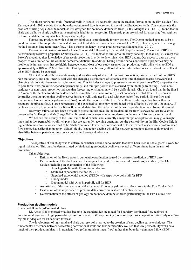
Table 2: Hindcast cumulative production error until end of known history

Table 3: Hindcast cumulative production error until end of known history, first six months omitted

Figure 10: Average hindcast error, including first six months

Forecast methods

18 months 24 months 30 months 36 months

Terminal decline -15.35% -16.73% -8.62% -10.22%

SEPD -6.73% -10.10% -6.04% -6.70%SEPD/Arps 10% Decline -6.93% -10.30% -6.81% -7.09%

SEPD/Arps 15% Decline -17.82% -15.37% -8.31% -7.57%

Duong 27.11% 14.12% 4.63% 6.12%

Duong/Arps 10% Decline 22.50% 11.28% 4.04% 6.27%


Time used for hindcast

Hindcast Individual Wells (Error to end of history), include first six months

Forecast methods


Terminal decline 0.48% 1.87% 0.01% 1.97%

SEPD -7.13% -5.35% -4.86% -2.86%



Duong 0.80% 5.29% 3.30% 7.66%


Duong/Arps 15% Decline -0.32% 4.87% 3.08% 6.05%

Time used for hindcast

Hindcast Individual Wells (Error to end of history), omit first six months



10 SPE-169018-MS

Figure 11: Average hindcast error, ignoring first six months

Figure 12: Standard deviation of hindcast error, including first six months



SPE-169018-MS 11

Figure 13: Standard deviation of hindcast error, ignoring first six months

Hindcasting with All Available Rate Data

First we will discuss hindcasts with the first six months included in the fit, as in Figure 14. The SEPD method is the most

accurate if only 18 months of data is used. However, the modified Duong method, with a switch to BDF at 15% decline, is the

most accurate if 24, 30, or 36 months of history is used in the fit. The Arps method with 5% terminal decline rate is the most

inaccurate method except in the case of using 18 months of history for the fit. The Arps method and the stretched exponential

method show a tendency to have too conservative a hindcast while the Duong method is too optimistic.

It can be seen that the average standard deviation in hindcast error decreases with the length of time used in the hind cast

except the 36 month hindcast. It is possible that this set of hindcasts has a greater variation in accuracy due to the beginning ofdeviation from linear flow.

Figure 14: Sample Elm Coulee well, hindcast beginning after two years

Hindcasting without First Six Months

Overall, we found that omitting the first six months of production history in a fit was beneficial, as in Figure 15. The

most dramatic difference caused by omitting the first six months of production history may be seen in early forecasts (18 to 24

months) using the Duong method. Later forecasts using the Duong method show a much less noticeable effect when ignoring the

first six months of data. With 36 months of production history available for the fit, omitting the first six months actually made the

hindcast a little worse than including it.



12 SPE-169018-MS

Figure 15: Sample Elm Coulee well, hindcast beginning after two years, first six months omitted

The Arps method with 5% minimum decline shows a dramatic increase in accuracy by omitting the first six months forall time periods studied, though not as much as the Duong method in early time. Without the first six months the SEPD and

SEPD/Arps hindcasts improved in most cases as well, but to a lesser extent than the other forecasting methods.

Similar to the hindcasts that included the first six months, the hindcasts that omitted this time period have an average

standard deviation in hindcast error that decreases with the length of time used in the hind cast up except in the case of the 36

month hindcast.

Grouped well hindcasts

We grouped production from all of the wells together and hindcasted on the data as if it were a single well. The grouped

well hindcast errors are, with or without using the first six months of production history, are shown in Table 4 and Table 5. We

summed the 154 well production data out to 59 months, the length of the shortest well history in the set. This is an effective way

of minimizing statistical and operational variation in wells that are expected to have similar production characteristics, based on

completion type, geology, pay thickness, produced fluids, etc. If there are enough wells in the Elm Coulee field, then groupingthem together should reduce statistical variation.

Since we are studying horizontal multi-fractured wells in the same formation, the wells should have similar decline

trends throughout the play. Grouping the data creates a smooth curve that can be fit more reliably. There is a great amount of

variation between wells, as has been seen, but there is less noticeable fluctuation between months of production.

Table 4: Elm Coulee grouped well hindcast, cumulative production error to the end of history

Forecast Methods


5% min. decline -23.46% -12.30% -9.09% -5.37%

SEPD -34.64% -6.68% -6.05% -2.57%

SEPD/Arps -34.64% -6.68% -6.05% -2.57%

Duong 34.63% 21.66% 13.95% 11.08%

Duong/Arps 34.63% 21.66% 13.95% 11.08%

Hindcast of Grouped wells (Error to end of history), include first six months

Time period used for hindcast



SPE-169018-MS 13

Table 5: Elm Coulee grouped well hindcast, cumulative production error to the end of history, first six months omitted

The grouped well hindcasts actually have more error than the average error for the individual well hindcasts. This may

be caused by the great variation in decline trends between wells. For the group hindcast, the Arps model with 5% minimum

decline did not have the lowest error, contrary to what was found in the single well hindcast results. Assuming the first six months

of history was omitted, the Duong method was the most accurate at 18 months of history and the SEPD method was the most

accurate method after that time. Even with hindcasting the wells as one group, using first six months of production history in thehindcast introduced significantly more error than if it was ignored, illustrated in the differences between Figure 16 and Figure 17.

Figure 16: Elm Coulee grouped well hindcast after first two years, ignoring first six months of history

Figure 17: Elm Coulee grouped well hindcast after first two years

Forecast Methods


5% min. decline 8.90% 9.00% 5.51% 6.26%

SEPD 5.90% 0.87% -5.10% -1.50%

SEPD/Arps 5.90% 0.87% -5.10% -1.50%

Duong 2.03% 7.56% 7.55% 8.94%

Duong/Arps 2.03% 7.56% 7.55% 8.94%

Hindcast of Grouped wells (Error to end of history), ignore first six months

Time period used for hindcast



14 SPE-169018-MS

Boundary-dominated flow analysis

While the previous hindcast study indicated how the decline curve methods may be applied to wells in transient flow, a

study of wells in boundary-dominated flow is necessary in order to determine how well the SEPD/Arps and Duong/Arps methods

work. Figure 18 shows production from lease Toni 2-17H, in the Elm Coulee field which we will use as an example.

Figure 18: TONI 2-17H , Rate versus time

Figure 19: TONI 2-17H, Production rate versus time plot

Figure 19 shows log-oil flow-rate versus log-time. The change is evident from negative half-slope, indicating linear flow,

to a negative unit slope of log-rate versus log-time, indicating boundary-dominated flow. It is unclear from this graph the exact

time at which the change occurs. There is a significant amount of scatter at the end of the production history, above and below the

expected trend. This obscures the trend somewhat. Since the production occurs both above and below the expected BDF trend, we

have assumed that boundary flow has occurred despite possible well interventions at the end.



SPE-169018-MS 15

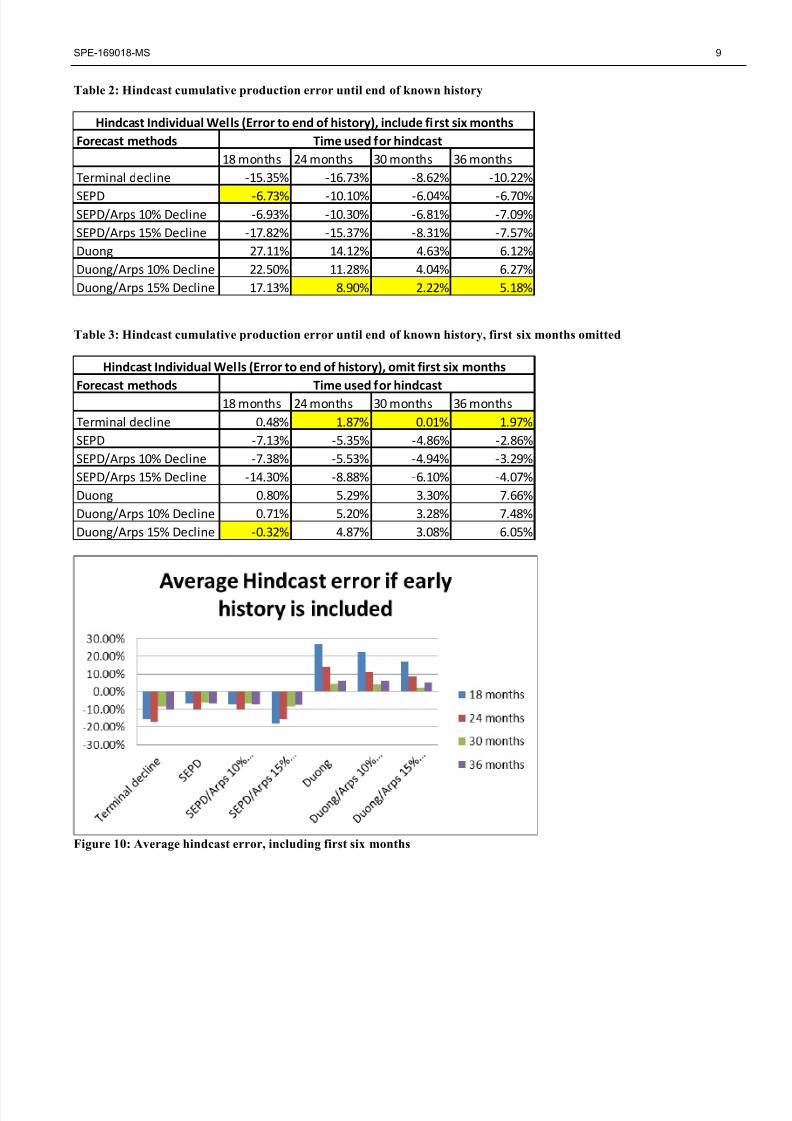
Figure 20: TONI 2-17H, Production rate versus material balance time diagnostic plot

The log-oil production rate versus material balance time plot in Figure 20 shows the onset of boundary-dominated flow

occurring around 132 N p/q months. This correlates to 61 months in actual time. This graph would be more accurate if bottomhole

pressure data were available to change rate into pressure-normalized rate.

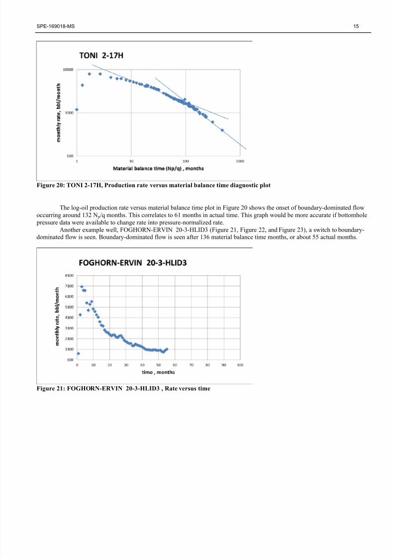
Another example well, FOGHORN-ERVIN 20-3-HLID3 (Figure 21, Figure 22, and Figure 23), a switch to boundary-dominated flow is seen. Boundary-dominated flow is seen after 136 material balance time months, or about 55 actual months.

Figure 21: FOGHORN-ERVIN 20-3-HLID3 , Rate versus time



16 SPE-169018-MS

Figure 22: FOGHORN-ERVIN 20-3-HLID3, Production rate versus time plot

Figure 23: FOGHORN-ERVIN 20-3-HLID3, Production rate versus material balance time diagnostic plot

Hindcasting with two years of data, the Duong method overestimates production while the terminal decline method

underestimates it. The SEPD method gives the closest hindcast. This is true whether the first six months are included or not.

Ignoring the first six months slightly increases the accuracy of the Duong method and slightly increases the error in the terminal

decline model as shown in Figure 24 and Figure 25.



SPE-169018-MS 17

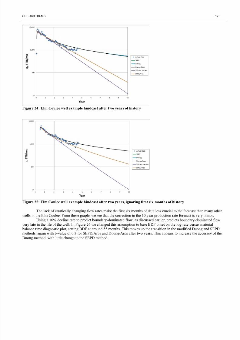
Figure 24: Elm Coulee well example hindcast after two years of history

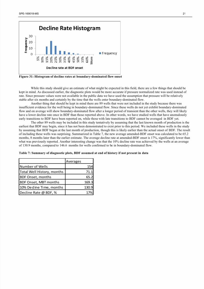
Figure 25: Elm Coulee well example hindcast after two years, ignoring first six months of history

The lack of erratically changing flow rates make the first six months of data less crucial to the forecast than many other

wells in the Elm Coulee. From these graphs we see that the correction in the 10 year production rate forecast is very minor.

Using a 10% decline rate to predict boundary-dominated flow, as discussed earlier, predicts boundary-dominated flow

very late in the life of the well. In Figure 26 we changed this assumption to base BDF onset on the log-rate versus material

balance time diagnostic plot, setting BDF at around 55 months. This moves up the transition in the modified Duong and SEPDmethods, again with b-value of 0.3 for SEPD/Arps and Duong/Arps after two years. This appears to increase the accuracy of the

Duong method, with little change to the SEPD method.



18 SPE-169018-MS

Figure 26: Elm Coulee well example hindcast after two years, ignoring first six months of history, BDF onset at 55 months

Figure 27: Elm Coulee well example hindcast after three years, ignoring first six months of history

Figure 28: Elm Coulee well example hindcast after three years, ignoring first six months, BDF onset at 55 months



SPE-169018-MS 19

Figure 25 shows the forecast without the predetermined BDF onset and Figure 26 shows BDF assumed to start at 55

months. Both the SEPD/Arps and the Duong/Arps create hindcasts that improve the accuracy of the SEPD or the Duong methods.

Figure 27 and Figure 28 similarly show BDF onset 10% decline and 55 months respectively, but begin the hindcast after 3 years.

We can postulate that rather than setting a decline rate at which to set the beginning of boundary-dominated flow, it

would be better to have an estimate of when boundary-dominated flow should occur based on reservoir and well properties, as

explained by Nobakht, et al, (2010). While these properties were not available for most wells in this study, operating companies

should have access to this data for their own wells and be able to use it rather than relying on decline rates to predict the start of

boundary-dominated flow.

Study of boundary-dominated flow onset in Elm Coulee field

We performed a further analysis on all of the wells used in the previous study of the Elm Coulee field. While there waslittle difference between the hindcasts that accounted for the switch to boundary-dominated flow (BDF) and those that did not, we

should expect this difference to increase later in the life of the wells.

We found that 65 of the 154 wells appear to have reached BDF by the end of known production history. In order to

diagnose BDF We used a log-production versus log-material balance time plot for each well. Material balance time is calculated

as cumulative production divided by production rate (N p/q). A negative half slope is indicative of linear flow, while a negative

unit slope is indicative of BDF, as shown in Figure 29.

Figure 29: Production rate versus material balance time diagnostic plot

In order to smooth the production data for our assessment we fit an Arps curve to the production data using an Excel

Solver. We omitted the first six months of production data, as we had found that this increased the accuracy of hindcasts. For this

exercise it is not important for the decline curve to model BDF, but should give a more accurate fit since the trend will mostly be

in linear flow until the time BDF begins. Not surprisingly, the Arps decline model in the Figure 30 does not fit the very early or

late data properly. The fit has a b-value of about 0.6.



20 SPE-169018-MS

Figure 30: Production rate versus material balance time diagnostic plot, fitted with Arps decline model

In many cases the onset of BDF may be seen clearly by visual inspection with a unit slope line. To create a moreconsistent analysis we fit an Arps curve to the production data, ignoring the first six months; we calculated the slope of the log-

production versus log-material balance time at each time, from that point until the end of the production history, including all

points in between. At the onset of BDF the log-log slope of all the following production data points should be approximately

equal to -1. Using this criteria we picked the point at which the calculated slope to the end of production began to be consistently

near -1 as the onset of boundary-dominated flow. In addition, boundary-dominated flow onset was assumed only if 1/3 of a log-

cycle of the well history showed a slope near -1. For this study we considered slopes of between -0.9 and -1.1 to be “near”

boundary-dominated flow. Since there is constant fluctuation in the production rate it is necessary to establish an interval during

which boundary-dominated flow is likely.

The results of this study, shown in Table 6, showed 65 wells in boundary-dominated flow. The wells produced for an

average of 71.2 months and boundary-dominated flow occurred at about 57.2 months, approximately a year before the end of

production. The time at which 10% decline was predicted to occur, according to the decline curve fit, was after an average of146.6 months, significantly later than shown by these wells. The actual decline rate at BDF onset averaged 22%.

Table 6: Summary of diagnostic plots

The 22% decline rate at BDF onset is much higher than the 10% that was assumed for the hindcast study. The histogram

below, Figure 31, shows that the most common decline rate for BDF onset was between 15% and 20%. There are several outliersthat entered BDF at continuous decline rates of up to 46% per year.

Averages

Number of wells in BDF 65

Total Well History, months 71.2

BDF Onset, months 57.2

BDF Onset, MBT months 169.8

10% Decline Time, months 146.6

Decline Rate @ BDF, % 22%



SPE-169018-MS 21

Figure 31: Histogram of decline rates at boundary-dominated flow onset

While this study should give an estimate of what might be expected in this field, there are a few things that should be

kept in mind. As discussed earlier, the diagnostic plots would be more accurate if pressure normalized rate was used instead of

rate. Since pressure values were not available in the public data we have used the assumption that pressure will be relatively

stable after six months and certainly by the time that the wells enter boundary-dominated flow.Another thing that should be kept in mind there are 89 wells that were not included in the study because there was

insufficient evidence for the well being in boundary-dominated flow. Since these wells do not yet exhibit boundary-dominated

flow and on average will show boundary-dominated flow after a longer period of transient than the other wells, they will likelyhave a lower decline rate once in BDF than those reported above. In other words, we have studied wells that have anomalously

early transitions to BDF have been reported on, while those with late transitions to BDF cannot be averaged in BDF yet.

The other 89 wells may be included in this study tentatively by assuming that the last known month of production is the

earliest that BDF may begin, since it has not been demonstrated to exist prior to this period. We included these wells in the study

by assuming that BDF began at the last month of production, though this is likely earlier than the actual onset of BDF. The result

of including these wells was surprising. Summarized in Table 7, the new average amended-BDF onset was calculated to be 65.2

months, 8 months later than the earlier estimate. The average decline rate at amended-BDF onset is 17%, significantly lower than

what was previously reported. Another interesting change was that the 10% decline rate was achieved by the wells at an average

of 130.9 months, compared to 146.6 months for wells confirmed to be in boundary-dominated flow.

Table 7: Summary of diagnostic plots, BDF assumed at end of history if not present in data

Averages

Number of Wells 154

Total Well History, months 71.1

BDF Onset, months 65.2

BDF Onset, MBT months 169.3

10% Decl ine Time, months 130.9

Decline Rate @ BDF, % 17%



22 SPE-169018-MS

Figure 32: Histogram of decline rates at boundary-dominated flow onset, amended study

While it is preferable to estimate the time when boundary-dominated flow begins from reservoir data, using a switch at a

certain decline rate can give an estimate of when this might occur. This will be important for economic considerations early in thedevelopment of a field. When there is high uncertainty in ultimate recovery it may be adequate to ask what is reasonable rather

than what is expected. Figure 32 shows that assuming decline rate at BDF will has a very wide range. It may be helpful to

quantify uncertainty for BDF onset to deal with the wide range of possible outcomes.

Unexpected deviations from linear flow

This study has assumed that the linear flow trend ends at the time that fracture interference begins. Another cause of boundary-dominated flow onset could occur in wells drilled near a fault or pinchout. In this case the radius of investigation from

the fracture may reach the boundary before the flow from different fractures interfere with each other. These cases should be rare,

but may skew assumptions of when fracture interference will occur.

Another cause for a unit slope to appear on the material balance time plot is a malfunction of the production equipment.

This will cause a sharp deviation from the assumed linear flow trend. This lowered rate will appear to be boundary-dominated

flow, creating a false assumption of fracture interference or a nearby boundary.

Conclusions

On average, the most accurate method found of fitting known production history in the Elm Coulee field is implementing

the Arps hyperbolic equation while ignoring the first six months of production.

The Duong method was the second most accurate method in fitting known data if the first six months are ignored. The

Duong method was also the most reliable method. Using the Duong method with an Arps modification for BDF may be

the best method for predicting production in these formations.

Methods used for shale gas forecasting have been shown to be applicable to shale oil or tight oil formations as well: Arps

method with 5% minimum decline, the stretched exponential method (SEPD), and the Duong method were found to be

useful in predicting transient flow production in shale oil wells as shown from hindcasts in the Elm Coulee field. The

Arps and Duong methods required that the early production history be removed from the fit in order to accurately model

linear flow.

Boundary-dominated flow was observed in diagnostic plots of wells in the Elm Coulee field in 65 wells out of the 154

wells studied. This was determined by finding at least 1/3 of a log cycle of data with negative unit slope on a rate versusmaterial balance time diagnostic plot.

The average decline rate at BDF onset of wells shown to be in boundary-dominated flow was about 22%. However,

since these were the early BDF onset cases, the actual average for all the wells in this field will likely be less than 17%.

Some occurrences of boundary-dominated flow may be due to production problems or wells near faults rather than

fracture interference.



SPE-169018-MS 23

References

Alexandre, C.S., Sonnenberg, S., and Sarg, J.F. 2012. Diagenesis of the Bakken Formation, Elm Coulee Field, Richland County,

Montana. In AAPG Annual Convention and Exhibition. Long Beach, California, USA: AAPG.

Ambrose, R.J., Clarkson, C.R., Youngblood, J.E. et al. 2011. Life-Cycle Decline Curve Estimation for Tight/Shale Reservoirs.

Paper presented at the SPE Hydraulic Fracturing Technology Conference, The Woodlands, Texas, USA. Society of

Petroleum Engineers SPE-140519-MS. DOI: 10.2118/140519-ms.

Arps, J.J. 1945. Analysis of Decline Curves. AIME 160: 228-247.Borglum, S.J. and Todd, B.J. 2012. An Investigation of Ancient Geological Events and Localized Fracturing on Current Bakken

Production Trends. Paper presented at the SPE Eastern Regional Meeting, Lexington, Kentucky, USA. Society of

Petroleum Engineers SPE-161331-MS. DOI: 10.2118/161331-ms.Chu, L., Ye, P., Harmawan, I.S. et al. 2012. Characterizing and Simulating the Nonstationariness and Nonlinearity in

Unconventional Oil Reservoirs: Bakken Application. Paper presented at the SPE Canadian Unconventional Resources

Conference, Calgary, Alberta, Canada. Society of Petroleum Engineers SPE-161137-MS. DOI: 10.2118/161137-ms.

Duong, A.N. 2010. An Unconventional Rate Decline Approach for Tight and Fracture-Dominated Gas Wells. Paper presented at

the Canadian Unconventional Resources and International Petroleum Conference, Calgary, Alberta, Canada. Society of

Petroleum Engineers 137748-MS.

Ilk, D., Currie, S.M., Symmons, D. et al. 2010. Hybrid Rate-Decline Models for the Analysis of Production Performance in

Unconventional Reservoirs. Paper presented at the SPE Annual Technical Conference and Exhibition, Florence, Italy.

Society of Petroleum Engineers 135616-MS.

Joshi, K. and Lee, W.J. 2013. Comparison of Various Deterministic Forecasting Techniques in Shale Gas Reservoirs. Paper presented at the 2013 SPE Hydraulic Fracturing Technology Conference, The Woodlands, Texas, USA. Society of

Petroleum Engineers SPE-163870-MS. DOI: 10.2118/163870-ms.Kurtoglu, B., Cox, S.A., and Kazemi, H. 2011. Evaluation of Long-Term Performance of Oil Wells in Elm Coulee Field. Paper

presented at the Canadian Unconventional Resources Conference, Alberta, Canada. Society of Petroleum Engineers

SPE-149273-MS. DOI: 10.2118/149273-ms.

Luo, S., Neal, L., Arulampalam, P. et al. 2010. Flow Regime Analysis of Multi-Stage Hydraulically-Fractured Horizontal Wells

with Reciprocal Rate Derivative Function: Bakken Case Study. Paper presented at the Canadian Unconventional

Resources and International Petroleum Conference, Calgary, Alberta, Canada. Society of Petroleum Engineers 137514-

MS.

Mangha, V.O., Ilk, D., Blasingame, T.A. et al. 2012. Practical Considerations for Decline Curve Analysis in Unconventional

Reservoirs --- Application of Recently Developed Rate-Time Relations. Paper presented at the SPE Hydrocarbon

Economics and Evaluation Symposium, Calgary, Alberta, Canada. Society of Petroleum Engineers SPE-162910-MS.

DOI: 10.2118/162910-ms.

Nobakht, M., Mattar, L., Moghadam, S. et al. 2010. Simplified yet Rigorous Forecasting of Tight/Shale Gas Production in LinearFlow. Paper presented at the SPE Western Regional Meeting, Anaheim, California, USA. Society of Petroleum

Engineers 133615-MS.

Tran, T., Sinurat, P.D., and Wattenbarger, B.A. 2011. Production Characteristics of the Bakken Shale Oil. Paper presented at the

SPE Annual Technical Conference and Exhibition, Denver, Colorado, USA. Society of Petroleum Engineers SPE-

145684-MS. DOI: 10.2118/145684-ms.

V. Hough, E. and McClurg, T. 2011. Impact of Geological Variation and Completion Type in the U.S. Bakken Oil Shale Play

Using Decline Curve Analysis and Transient Flow Character. In AAPG International Conference and Exhibit . Milan,

Italy.

Valko, P.P. and Lee, W.J. 2010. A Better Way to Forecast Production from Unconventional Gas Wells. Paper presented at the

SPE Annual Technical Conference and Exhibition, Florence, Italy. Society of Petroleum Engineers 134231-MS.

Walker, B., Powell, A., Rollins, D. et al. 2006. Elm Coulee Field Middle Bakken Member (Lower Mississippian/UpperDevonian) Richland County, Montana. In AAPG Rocky Mountain Section meeting . Billings, Montana: AAPG.

Documents

A Study of Decline Curve