A Structured Multiarmed Bandit Problemand the Greedy Policy

Adam J. MersereauKenan-Flagler Business School, University of North Carolina

ajm@unc.edu

Paat RusmevichientongSchool of Operations Research and Information Engineering, Cornell University

paatrus@cornell.edu

John N. TsitsiklisLaboratory for Information and Decision Systems, Massachusetts Institute of Technology

jnt@mit.edu

We consider a multiarmed bandit problem where the expected reward of each arm is a linear function of an

unknown scalar with a prior distribution. The objective is to choose a sequence of arms that maximizes the

expected total (or discounted total) reward. We demonstrate the effectiveness of a greedy policy that takes

advantage of the known statistical correlation structure among the arms. In the infinite horizon discounted

reward setting, we show that the greedy and optimal policies eventually coincide, and both settle on the

best arm. This is in contrast with the Incomplete Learning Theorem for the case of independent arms. In

the total reward setting, we show that the cumulative Bayes risk after T periods under the greedy policy

is at most O (logT ), which is smaller than the lower bound of Ω`log2 T

´established by Lai (1987) for a

general, but different, class of bandit problems. We also establish the tightness of our bounds. Theoretical

and numerical results show that the performance of our policy scales independently of the number of arms.

1. Introduction

In the multiarmed bandit problem, a decision-maker samples sequentially from a set of m

arms whose reward characteristics are unknown to the decision-maker. The distribution of

the reward of each arm is learned from accumulated experience as the decision-maker seeks

to maximize the expected total (or discounted total) reward over a horizon. The problem

has garnered significant attention as a prototypical example of the so-called exploration ver-

sus exploitation dilemma, where a decision-maker balances the incentive to exploit the arm

with the highest expected payoff with the incentive to explore poorly understood arms for

information-gathering purposes.

Nearly all previous work on the multiarmed bandit problem has assumed statistically inde-

pendent arms. This assumption simplifies computation and analysis, leading to multiarmed

bandit policies that decompose the problem by arm. The landmark result of Gittins and Jones

(1974), assuming an infinite horizon and discounted rewards, shows that an optimal policy

1

2

always pulls the arm with the largest “index,” where indices can be computed independently

for each arm. In their seminal papers, Lai and Robbins (1985) and Lai (1987) further show

that index-based approaches achieve asymptotically optimal performance in the finite horizon

setting when the objective is to maximize total expected rewards.

When the number of arms is large, statistical independence comes at a cost, because it

typically leads to policies whose convergence time increases with the number of arms. For

instance, most policies require each arm be sampled at least once. At the same time, statistical

independence among arms is a strong assumption in practice. In many applications, we expect

that information gained by pulling one arm will also impact our understanding of other

arms. For example, in a target marketing setting, we might expect a priori that similar

advertisements will perform similarly. The default approach in such a situation is to ignore

any knowledge of correlation structure and use a policy that assumes independence. This

seems intuitively inefficient because we would like to use any known statistical structure to

our advantage.

We study a fairly specific model that exemplifies a broader class of bandit problems where

there is a known prior functional relationship among the arms’ rewards. Our main thesis

is that known statistical structure among arms can be exploited for higher rewards and

faster convergence. Our assumed model is sufficient to demonstrate this thesis using a simple

greedy approach in two settings: infinite horizon with discounted rewards, and finite horizon

undiscounted rewards. In the discounted reward setting, we show that the greedy and optimal

policies eventually coincide, and both settle on the best arm in finite time. This differs from

the classical multiarmed bandit case, where the Incomplete Learning Theorem (Rothschild

1974, Banks and Sundaram 1992, Brezzi and Lai 2000) states that no policy is guaranteed

to find the best arm. In the finite horizon setting, we show that the cumulative Bayes risk

over T periods (defined below) under the greedy policy is bounded above by O(logT ) and is

independent of the number of arms. This is in contrast with the classical multiarmed bandit

case where the risk over T periods is at least Ω(log2 T ) (Lai 1987), and typically scales linearly

with the number of arms. We outline our results and contributions in more detail in Section

1.2.

Our formulation assumes that the mean reward of each arm is a linear function of an

unknown scalar on which we have a prior distribution. Assume that we have m arms indexed

by 1, . . . ,m, where the reward for choosing arm ` in period t is given by a random variable

X t` . We assume that for all t≥ 1 and for `= 1, . . . ,m, X t

` is given by

X t` = η` +u`Z +Et

` , (1)

3

where η` and u` are known for each arm `, and Z and Et` : t ≥ 1, ` = 1, . . . ,m are

random variables. We will assume throughout the paper that for any given `, the ran-

dom variables Et` : t≥ 1 are identically distributed; furthermore, the random variables

Et` : t≥ 1, `= 1, . . . ,m are independent of each other and of Z.

Our objective is to choose a sequence of arms (one at each period) so as to maximize either

the expected total or discounted total rewards. Define the history of the process, Ht−1, as the

finite sequence of arms chosen and rewards observed through the end of period t−1. For each

t≥ 1, let Ht−1 denote the set of possible histories up until the end of period t− 1. A policy

Ψ = (Ψ1,Ψ2, . . .) is a sequence of functions such that Ψt :Ht−1→1,2, . . . ,m selects an arm

in period t based on the history up until the end of period t− 1. For each policy Ψ, the total

discounted reward is given by

E

[∞∑t=1

βtX tJt

],

where 0< β < 1 denotes the discount factor, and the random variables J1, J2, . . . correspond

to the sequence of arms chosen under the policy Ψ, that is, Jt = Ψt(Ht−1). For every T ≥ 1,

we define the T -period cumulative regret under Ψ given Z = z, denoted by Regret(z,T,Ψ),

as follows

Regret(z,T,Ψ) =T∑t=1

E

[max

`=1,...,m(η` +u`z)− (ηJt +uJtz)

∣∣∣ Z = z

],

and the T -period cumulative Bayes risk of the policy Ψ by

Risk (T,Ψ) = EZ [Regret (Z,T,Ψ)] .

We note that maximizing the expected total reward over a finite horizon is equivalent to

minimizing Bayes risk.

Although this is not our focus, we point out an application of our model in the area of

dynamic pricing with demand learning. Assume that we are sequentially selecting from a

finite set P of prices with the objective of maximizing revenues over a horizon. When the

price p` ∈ P is selected at time t, we assume that sales St` are given by the linear demand

curve

St` = a− bp` + εt`,

where a is a known intercept but the slope b is unknown. The random variable εt` is a noise

term with mean zero. The revenue is then given by Rt` = p`S

t = ap`−p2`b−p`εt`, which is a spe-

cial case of our model. We mention this dynamic pricing problem as an example application,

4

though our model is more generally applicable to a range of control situations involving a lin-

ear function to be estimated. Example application domains include drug dosage optimization

(Lai and Robbins 1978), natural resource exploration, and target marketing.

1.1. Related Literature

As discussed in Section 1, work on the multiarmed bandit problem has typically focused on

the case where the arm rewards are assumed to be statistically independent. The literature

can be divided into two streams based on the objective function: maximizing the expected

total discounted reward over an infinite horizon and minimizing the cumulative regret or

Bayes risk over a finite horizon. Our paper contributes to both streams of the literature.

In the discounted, infinite horizon setting, the landmark result of Gittins and Jones (1974)

shows that an index-based policy is optimal under geometric discounting. Several alternative

proofs of the so-called Gittins Index result exist (Whittle 1980, Weber 1992, Tsitsiklis 1994,

Bertsimas and Nino-Mora 1996); see Frostig and Weiss (1999) for a summary and review. The

classical Gittins assumptions do not hold in our version of the problem because statistical

dependence among arms does not allow one to compute indices for each arm in a decomposable

fashion. In the discounted setting, it is known (Rothschild 1974, Banks and Sundaram 1992,

Brezzi and Lai 2000) that learning is incomplete when arms are independent. That is, an

optimal policy has a positive probability of never settling on the best arm.

A second stream of literature has sought to maximize the expected total undiscounted

reward or, equivalently, to minimize regret, defined as expected underperformance of a policy

relative to the policy that knows and always chooses the best arm. A full characterization

of an optimal policy given this objective appears to be difficult, and most authors have

concerned themselves with rates of convergence of particular policies. The seminal work of

Lai and Robbins (1985) gives an asymptotic Ω(logT ) lower bound on the regret as a function

of time. It also provides a policy based on “upper confidence bounds” on the arm rewards,

whose performance asymptotically matches the lower bound. Lai (1987) extends these results

and shows, among other things, that in a Bayesian finite horizon setting, and under a fairly

general set of assumptions, the cumulative Bayes risk must grow at least as fast as Ω(log2 T

).

Subsequent papers along this line include Agrawal et al. (1989), Agrawal (1996), and Auer

et al. (2002a).

Interest in bandit problems under an assumption of dependent arms has a long history.

Thompson (1933), in what is widely regarded as the original paper on the multiarmed bandit

problem, allows for correlation among arms in his initial formulation, though he only analyzes

5

a special case involving independent arms. Robbins (1952) formulates a continuum-armed

bandit regression problem that subsumes our model, but does not provide an analysis of

regret or risk. The formulation in Chapter 2 of Berry and Fristedt (1985) allows for correlation

among arms (though most of the book concerns cases with independent arms). There has

been relatively little analysis, however, of bandit problems with dependent arms. Feldman

(1962) and Keener (1985) consider two-armed bandit problems with two hidden states, where

the rewards for each arm depend on which of the underlying states prevails. Pressman and

Sonin (1990) formulate a general multiarmed bandit problems with an arbitrary number of

hidden states, and provide a detailed analysis for the case of two hidden states. Ginebra

and Clayton (1995) formulate “response surface bandits,” multiarmed bandit problems whose

arm rewards are linked through an assumed functional model, and they provide a simple

tunable heuristic. Pandey et al. (2007) study bandit problems where the dependence of the

arm rewards is represented via a hierarchical model. Tewari and Bartlett (2008) develop a

policy that aims to maximize the average reward in an irreducible (but unknown) Markov

decision process (MDP); their policy admits logarithmic regret but scales linearly with the

number of actions and states of the underlying MDP.

Our model can be viewed as a special case of an online convex optimization problem, by

considering randomized decisions. Let S = p∈ [0,1]m :∑m

`=1 p` = 1 denote an m-dimensional

simplex, where each p = (p1, . . . , pm) ∈ S can be interpreted as the probabilities of play-

ing the m arms. Given Z = z, the expected reward under a decision p ∈ S is given by∑m`=1 p` (η` +u`z), which is linear in p. For a bounded linear reward function on an m-

dimensional decision space, Kleinberg (2008) proposes a policy whose cumulative regret over

T periods is at most O(m5/3T 2/3

)(see also, McMahan and Blum 2004 and Dani and Hayes

2006). Kleinberg (2005) and Flaxman et al. (2005) further generalize this result to convex cost

functions, obtaining policies whose T -period regret is O(m T 3/4

). Nearly all of the work in

this area focuses on minimizing regret, and all known policies have regret that scales with the

dimension of the problem space (corresponding to the number of arms m in our setting). By

exploiting the specific structure of our reward function, however, we can get a stronger result

and obtain a policy whose cumulative regret over T periods is only O(√T ). Moreover, our

regret bound is independent of m (Theorem 3.1 in Section 3). We also consider the discounted

reward and cumulative Bayes risk criteria.

We presented in Section 1 an application of our model to dynamic pricing with learning.

Although this is not a focus of the current paper, we mention that there is a growing literature

6

on this specific topic. See Carvalho and Puterman (2004), Aviv and Pazgal (2005), Farias and

Van Roy (2006), and Besbes and Zeevi (2006) for examples of recent work. All of these models

are distinguished from ours in their objectives and in the specific demand and inventory

situations treated.

1.2. Contributions and Organization

We view our main contributions to be (1) a model of statistical dependence among the arm

rewards, (2) analysis of such a model under both expected discounted and undiscounted

reward objectives, and (3) demonstration that prior knowledge of the statistical dependence

of the different arms can improve performance and scalability. To the best of our knowledge,

this is the first paper to provide detailed theoretical analysis of a multiarmed bandit model

where the arm rewards are correlated through a continuous random variable with known prior

distribution.

Section 2 includes our analysis of the infinite-horizon setting with geometric discounting.

Theorem 2.1 establishes our main result on “complete learning.” When every arm depends

on the underlying random variable Z (that is, if u` 6= 0 for all `), the posterior mean of Z

converges to its true value. We also show that a greedy decision is optimal when the variance

of the posterior distribution is sufficiently small (Theorem 2.2). These two results together

imply that eventually the optimal policy coincides with the greedy policy, and both settle on

the best arm (Theorem 2.3). As mentioned previously, the latter result relies on the assumed

correlation structure among the arms and is in contrast to the Incomplete Learning Theorem

for the classical multiarmed bandit setting. We conclude Section 2 by examining the case

where some of the coefficients u` are allowed to be zero. We argue that the corresponding

arms can be interpreted as “retirement options,” and prove that when retirement options are

present, the optimal and greedy policies may never coincide, and that learning is generally

incomplete.

In Section 3, we analyze a similar greedy policy in the finite horizon setting, under the

expected reward, or equivalently, cumulative Bayes risk criterion. We focus first on measuring

the regret of the greedy policy. We show in Theorem 3.1 that the cumulative regret over T

periods admits an O(√T ) upper bound and that this bound is tight. Although this leads

to an immediate O(√T ) upper bound on the cumulative Bayes risk, we show that we can

achieve an even smaller, O(logT ), cumulative Bayes risk bound, under mild conditions on

the prior distribution of Z (Theorem 3.2). The O(logT ) risk bound is smaller than the

known Ω(log2 T ) lower bound of Lai (1987), and we explain why our framework represents an

7

exception to the assumptions required in Lai (1987). Theorem 3.2 also shows that Bayes risk

scales independently of the number of arms m. This result suggests that when the number of

arms is large, we would expect significant benefits from exploiting the correlation structure

among arms. Numerical experiments in Section 4 support this finding.

2. Infinite Horizon With Discounted Rewards

In this section, we consider the problem of maximizing the total expected discounted reward.

For any policy Ψ, the expected total discounted reward is defined as E[∑∞

t=1 βtX t

Jt

], where

0< β < 1 denotes the discount factor and Jt denotes the arm chosen in period t under the

policy Ψ. We make the following assumption on the random variables Z and Et`.

Assumption 2.1.

(a) The random variable Z is continuous, and E [Z2]<∞. Furthermore, for every t and`, we have E [Et

`] = 0 and γ2` := E

[(Et

`)2 ]<∞.

(b) We have u` 6= 0, for every `.

(c) If k 6= `, then uk 6= u`.

Assumption 2.1(a) places mild moment conditions on the underlying random variables, while

Assumption 2.1(b) ensures that the reward of each arm is influenced by the underlying random

variable Z. In Section 2.3, we will explore the consequence of relaxing this assumption and

allow some of the coefficients u` to be zero. Finally, Assumption 2.1(c) is only introduced

for simplicity and results in no loss of generality. Indeed, if the coefficient u` is the same for

several arms, we should only consider playing one with the largest value of η`, and the others

can be eliminated.

In the next section, we show that “complete learning” is possible, under Assumption 2.1.

In Theorem 2.1, we show that the posterior mean of Z converges to its true value, under any

policy. This result then motivates us to consider in Section 2.2 a greedy policy that makes

a myopic decision based only on the current posterior mean of Z. We establish a sufficient

condition for the optimality of the greedy policy (Theorem 2.2), and show that both the

greedy and optimal policies eventually settle on the best arm, with probability one (Theorem

2.3). In contrast, when we allow some of the coefficients u` to be zero, it is possible for the

greedy and optimal policies to disagree forever, with positive probability (Theorem 2.5 in

Section 2.3).

8

2.1. Complete Learning

Let us fix an arbitrary policy Ψ, and for every t, let Ft be the σ-field generated by the history

Ht, under that policy. Let Yt be the posterior mean of Z, that is,

Yt = E[Z∣∣ Ft] ,

and let Vt be the conditional variance, that is,

Vt = E[(Z −Yt)2 | Ft

]= Var (Z | Ft) .

The following result states that, under Assumption 2.1, we have complete learning, for every

policy Ψ.

Theorem 2.1 (Complete Learning). Under Assumption 2.1, for every policy Ψ, Yt con-

verges to Z and Vt converges to zero, almost surely.

Proof: Let us fix a policy Ψ, and let J1, J2, . . . be the sequence of arms chosen under Ψ. The

sequence Yt is a martingale with respect to the filtration Ft : t≥ 0. Furthermore, since

E [Z2] <∞, it is a square integrable martingale. It follows that Yt converges to a random

variable Y , almost surely, as well as in the mean-square sense. Furthermore, Y is equal to

E[Z | F∞], where F∞ is the smallest σ-field containing Ft for all t (Durrett 1996).

We wish to show that Y =Z. For this, it suffices to show that Z is F∞-measurable. To this

effect, we define

Yt =1t

t∑τ=1

XτJτ− ηJτuJτ

=Z +1t

t∑τ=1

EτJτ

uJτ.

Then,

Var(Yt−Z) =1t2

t∑τ=1

γ2Jτ

u2Jτ

≤ max`(γ2` /u

2`)

t.

It follows that Yt converges to Z in the mean square. Since Yt belongs to F∞ for every t, it

follows that its limit, Z, also belongs to F∞. This completes the proof of convergence of Yt

to Z.

Concerning the conditional variance, the definition of Vt implies that Vt =

E[(Z −Yt)2 | Ft

]= E [Z2 | Ft]− Y 2

t , so that Vt is a nonnegative supermartingale. Therefore,

Vt converges almost surely (and thus, in probability) to some random variable V . Since

limt→∞ E[Vt] = 0, Vt also converges to zero in probability. Therefore, V = 0 with probability

one.

9

In our problem, the rewards of the arms are correlated through a single random variable

Z to be learned, and thus, we intuitively have only a “single” arm. Because uncertainty is

univariate, we have complete learning under any policy, in contrast to the Incomplete Learning

Theorem for the classical multiarmed bandit problems. As a consequence of Theorem 2.1, we

will show in Section 2.2 (Theorem 2.3) that an optimal policy will settle on the best arm with

probability one.

2.2. A Greedy Policy

From Theorem 2.1, the posterior mean of Z, under any policy, converges to the true value

of Z almost surely. This suggests that a simple greedy policy – one whose decision at each

period is based solely on the posterior mean – might perform well. A greedy policy is a policy

whose sequence of decisions(JG1 , J

G2 , . . .

)is defined by: for each t≥ 1,

JGt = arg max`=1,...,m

η` +u`E

[Z | FGt−1

],

whereFGt : t≥ 1

denotes the corresponding filtration; for concreteness, we assume that ties

are broken in favor of arms with lower index. Note that the decision JGt is a myopic one, based

only on the conditional mean of Z given the past observations up until the end of period t−1.

Intuitively, the quality of the greedy decision will depend on the variability of Z relative

to the difference between the expected reward of the best and second best arms. To make

this concept precise, we introduce the following definition. For any µ, let ∆(µ) denote that

difference between the reward of the best and the second best arms, that is,

∆(µ) = max`=1,...,m

η` +µu`− max`=1,...,m: `6=πG(µ)

η` +µu` ,

where πG(µ) = arg max`=1,...,m η` +µu`. Figure 1 shows an example of the function ∆(·) in

a setting with 4 arms. Note that ∆(·) is a continuous and nonnegative function. As seen from

Figure 1, ∆(µ) may be zero for some µ. However, given our assumption that the coefficients

u` are distinct, one can verify that ∆(µ) has at most m− 1 zeros.

The next theorem shows that, under any policy, if the posterior standard deviation is small

relative to the mean difference between the best and second best arms, then it is optimal

to use a greedy policy. This result provides a sufficient condition for optimality of greedy

decisions.

10

µ

TexPoint fonts used in EMF.Read the TexPoint manual before you delete this box.: AAAAAAA

L1 : !1 +"u1L3 : !3 +"u3L2 : !2 +"u2L4 : !4 +"u4

Difference between SOLID and DOTTEDCurves corresponds to

Figure 1 An example of ∆(·) with 4 arms.

Theorem 2.2 (Optimality of Greedy Decisions). Under Assumption 2.1, there exists

a constant δ that depends only on β and the coefficients u`, with the following property. If

we follow a policy Ψ until some time t− 1, and if

∆(E[Z∣∣ Ft−1

])√Var[Z∣∣ Ft−1

] > δ ,

then it is optimal to apply the greedy policy in period t. (Here, Ft−1 is the σ-field generated

by the history Ht−1.)

Proof: Let us fix a policy Ψ and some t ≥ 1, and define µt−1 = E [Z | Ft−1], which is the

posterior mean of Z given the observations until the end of period t−1. Let J∗ and R∗ denote

the greedy decision and the corresponding reward in period t, that is,

J∗ = arg max`=1,...,m

η` +u`E [Z | Ft−1]= arg max`=1,...,m

η` +u`µt−1 and R∗ = ηJ∗ +uJ∗µt−1.

We will first establish a lower bound on the total expected discounted reward (from time t

onward) associated with a policy that uses a greedy decision in period t and thereafter. For

each s≥ t−1, let MGs = E

[Z | FGs

]denote the conditional mean of Z under this policy, where

FGs is the σ-field generated by the history of the process when policy Ψ is followed for up

to time t− 1, and the greedy policy is followed thereafter, so that FGt−1 = Ft−1. Under this

policy, the expected reward at each time s≥ t is

E

[max

`=1,...,mη` +u`M

Gs−1

∣∣∣ Ft−1

]≥ max

`=1,...,mE[η` +u`M

Gs−1

∣∣∣ Ft−1

]

11

= max`=1,...,m

η` +u`E

[Z∣∣ Ft−1

]=R∗,

where we first used Jensen’s inequality, and then the fact that the sequence MGs , s≥ t− 1,

forms a martingale. Thus, the present value at time t of the expected discounted reward under

a strategy that uses a greedy decision in period t and thereafter is at least R∗/(1−β).

Now, consider any policy that differs from the greedy policy at time t, and plays some arm

k 6= J∗. Let Rk = ηk + ukE [Z | Ft−1] = ηk + ukµt−1 denote the immediate expected reward in

period t. The future rewards under this policy are upper bounded by the expected reward

under the best arm. Thus, under this policy, the expected total discounted reward from t

onward is upper bounded by

Rk +β

1−βE

[max

`=1,...,mη` +u`Z

∣∣∣ Ft−1

]= Rk +

β

1−βE

[max

`=1,...,m

η` +u`µt−1 +u` (Z −µt−1)

∣∣∣ Ft−1

]≤ Rk +

β

1−βmax

`=1,...,mη` +u`µt−1+

β

1−βE

[max

`=1,...,mu` (Z −µt−1 )

∣∣∣ Ft−1

]= Rk +

β

1−βR∗+

β

1−βE

[max

`=1,...,mu` (Z −µt−1 )

∣∣∣ Ft−1

].

Note that

E

[max

`=1,...,mu` (Z −µt−1 )

∣∣∣ Ft−1

]≤(

max`=1,...,m

|u`|)

E[|Z −µt−1|

∣∣ Ft−1

]≤(

max`=1,...,m

|u`|)√

E[(Z −µt−1)

2∣∣ Ft−1

]=(

max`=1,...,m

|u`|)√

Var(Z∣∣ Ft−1

)Thus, under this policy the present value at time t of the total discounted reward is upper

bounded by

Rk +β

1−βR∗+

β

1−β

(max

`=1,...,m|u`|)√

Var(Z∣∣ Ft−1

)Recall that the total discounted reward under the greedy policy is at least R∗/(1 − β).

Moreover, for any arm k 6= J∗,

R∗

(1−β)=R∗+

β

1−βR∗ ≥ (ηk +ukµt−1) + ∆ (µt−1) +

β

1−βR∗ =Rk + ∆ (µt−1) +

β

1−βR∗

where the inequality follows from the definition of ∆(·). Thus, comparing the expected dis-

counted rewards of the two policies, we see that a greedy policy is better than any policy that

takes a non-greedy action if

∆(µt−1) >β

1−β

(max

`=1,...,m|u`|)√

Var(Z∣∣ Ft−1

),

12

which is the desired result.

As a consequence of Theorem 2.2, we can show that the greedy and optimal policies both

settle on the best arm with probability one.

Theorem 2.3 (Agreement Between Greedy and Optimal Polices). Under Assump-

tion 2.1, an optimal policy eventually agrees with the greedy policy, and both settle on the

best arm with probability one.

Proof: Let J∗ denote the best arm for each Z, that is, J∗ = arg max` η` +u`Z. Since Z is a

continuous random variable and ∆(·) = 0 at finitely many points, we can assume that J∗ is

unique.

For the greedy policy, since E[Z | FGt

]converges to Z almost surely by Theorem 2.1, it

follows that the greedy policy will eventually settle on the arm J∗ with probability one.

Consider an optimal policy Π∗. Let M ∗t = E [Z | F∗t ], where F∗t denotes the filtration under

Π∗. By Theorem 2.1, M ∗t converges to Z almost surely, and thus, ∆(M ∗

t ) converges to a

positive number, almost surely. Also, Var (Z | F∗t ) converges to zero by Theorem 2.1. Thus,

the condition in Theorem 2.2 is eventually satisfied, and thus Π∗ eventually agrees with the

greedy policy, with probability one.

2.3. Relaxing Assumption 2.1(b) Can Lead to Incomplete Learning

In this section, we explore the consequences of relaxing Assumption 2.1(b), and allow the

coefficients u` to be zero, for some arms. We will show that, in contrast to Theorem 2.3, there

is a positive probability that the greedy and optimal policies disagree forever. To demonstrate

this phenomenon, we will restrict our attention to a setting where the underlying random

variables Z and Et` are normally distributed.

When Z and all Et` are normal, the posterior distribution of Z remains normal. We can

thus formulate the problem as a Markov Decision Process (MDP) whose state is characterized

by (µ, θ)∈R×R+, where µ and θ denote the posterior mean and the inverse of the posterior

variance, respectively. The action space is the set of arms. When we choose an arm ` at state

(µ, θ), the expected reward is given by r ((µ, θ) , `) = η`+u`µ. Moreover, the updated posterior

mean µ′ ((µ, θ) , `) and the inverse of the posterior variance θ′((µ, θ) , `) are given by

θ′((µ, θ) , `) = θ+u2`

γ2`

and µ′((µ, θ) , `) =θ

θ+u2`/γ

2`

µ+u2`/γ

2`

θ+u2`/γ

2`

(X t` − η`u`

),

where X t` denotes the observed reward in period t. We note that these update formulas can

also be applied when u` = 0, yielding µ′((µ, θ), `) = µ and θ′((µ, θ), `) = θ. The reward function

13

r((·, ·) , ·) in our MDP is unbounded because the state space is unbounded. However, as shown

in the following lemma, there exists an optimal policy that is stationary. The proof of this

result appears in Appendix A.

Lemma 2.4 (Existence of Stationary Optimal Policies). When the random vari-

ables Z and Et` are normally distributed, then a deterministic stationary Markov policy is

optimal; that is, there exists an optimal policy π∗ : R×R+→1, . . . ,m that selects a deter-

ministic arm π∗(µ, θ) for each state (µ, θ).

It follows from the above lemma that we can restrict our attention to stationary policies. If

u` = 0 for some `, then there is a single such `, by Assumption 2.1(c), and we can assume that

it is arm `= 1. Since we restrict our attention to stationary policies, when arm 1 is played,

the information state remains the same, and the policy will keep playing arm 1 forever, for

an expected discounted reward of η1/(1− β). Thus, arm 1, with u1 = 0, can be viewed as a

“retirement option.”

Note that in this setting a greedy policy πG : R×R+→1, . . . ,m is defined as follows: for

every (µ, θ)∈R×R+,

πG(µ, θ) = arg max`η` +u`µ ,

with ties broken arbitrarily. We have the following result.

Theorem 2.5 (Incomplete Learning). If the random variables Z and Et` are normally

distributed, and if η1 > max`:u` 6=0η` + u`µ for some µ ∈ R, then the optimal and greedy

policies disagree forever with positive probability. Furthermore, under either the optimal or

the greedy policy, there is positive probability of retiring even though arm 1 is not the best

arm.

Proof: Under the assumption η1 > max`:u` 6=0η` + u`µ for some µ ∈ R, there is an open

interval I = (a, b) with a < b such that whenever µ ∈ I, the greedy policy must retire, that

is, πG(µ, θ) = 1 for all µ ∈ I and θ ∈ R+. Outside the closure of I, the greedy policy does

not retire. Outside the closure of I, an optimal policy does not retire either because higher

expected rewards are obtained by first pulling arm ` with η` + u`µ > η1. Without loss of

generality, let us assume that u` > 0 for some `. A similar argument applies if we assume

u` < 0 for some `.

Fix some ε∈ (0, b−a), and let Aε = (b−ε, b) be an open interval at the right end of I. There

exists a combination of sufficiently small ε0 and θ0 (thus, large variance) such that when we

consider the set of states (µ, θ) ∈ Aε0 × (0, θ0), the expected long-run benefit of continuing

14

exceeds the gain from retiring, as can be shown with a simple calculation. The set of states

Aε0 × (0, θ0) will be reached with positive probability. When this happens, the greedy policy

will retire. On the other hand, the optimal policy will choose to explore rather than retire.

Let Mt denote the posterior mean in period t under the optimal policy. We claim that

once an optimal policy chooses to explore (that is, play an arm other than arm 1), there is

a positive probability that all posterior means in future periods will exceed b, in which case

the optimal policy never retires. To establish the claim, assume that Mt0 > b for some t0.

Let τ be the stopping time defined as the first time after t0 that Mt ≤ b. We will show that

Prτ =∞> 0, so that Mt stays outside I forever, and the optimal policy never retires.

Suppose, on the contrary, that Prτ <∞= 1. Since Mt is a square integrable martingale,

it follows from the Optional Stopping Theorem that E [M τ ] = M t0, which implies that b <

M t0 = E [M τ ] = E [M τ ; τ <∞] ≤ b, where the last inequality follows from the definition of

τ . This is a contradiction, which establishes that Prτ =∞> 0, and therefore the greedy

policy differs from the optimal one, with positive probability.

For the last part of the theorem, we wish to show that under either the optimal or the

greedy policy, there is positive probability of retiring even though arm 1 is not the best arm.

To establish this result, consider the interval I ′ =(a+ (b−a)

3, a+ 2(b−a)

3

)⊂ I, representing the

middle third of the interval I. There exists θ′ sufficient large (thus, small variance) such that

when we consider the states (µ, θ) ∈ I ′ × [θ′,∞), the expected future gain from exploration

is outweighed by the decrease in immediate rewards. These states are reached with positive

probability, and at such states, the optimal policy will retire. The greedy policy also retires

at such states because I ′ ⊆ I. At the time of retirement, however, there is positive probability

that arm 1 is not the best one.

We note that when η1 ≤max`:u` 6=0η` + u`µ for all µ ∈ R, one can verify that, as long as

ties are never broken in favor of retirement, neither the greedy or the optimal policy will ever

retire, so we can ignore the retirement option.

3. Finite Horizon With Total Undiscounted Rewards

We now consider a finite horizon version of the problem, under the expected total reward

criterion, and focus on identifying a policy with small cumulative Bayes risk. As in Section

2, a simple greedy policy performs well in this setting. Before we proceed to the statement

of the policy and its analysis, we introduce the following assumption on the coefficients u`associated with the arms and on the error random variables Et

`.

15

Assumption 3.1.

(a) There exist positive constants b and λ such that for every ` and x≥ 0,

Pr(|Et

`| ≥ x)≤ be−λx,

(b) There exist positive constants u and u such that for every `,

u≤ |u`| ≤ u .

We view b, λ, u and u as absolute constants, which are the same for all instances of the problem

under consideration. Our subsequent bounds will depend on these constants, although this

dependence will not be made explicit. The first part of Assumption 3.1 simply states that the

tails of the random variables |Et`| decay exponentially. It is equivalent to an assumption that

all |Et`| are stochastically dominated by a shifted exponential random variable.

The second part of the Assumption 3.1 requires, in particular, the coefficients u` to be

nonzero. It is imposed because if some u` is zero, then, the situation is similar to the one

encountered in Section 2.3: a greedy policy may settle on a non-optimal arm, with positive

probability, resulting in a cumulative regret that grows linearly with time. More sophisticated

policies, with active experimentation, are needed in order to guarantee sublinear growth of

the cumulative regret, but this topic lies outside the scope of this paper.

We will study the following variant of a greedy policy. It makes use of suboptimal (in the

mean squared error sense) but simple estimators Yt of Z, whose tail behavior is amenable to

analysis. Indeed, it is not clear how to establish favorable regret bounds if we were to define

Yt as the posterior mean of Z.

Greedy Policy for Finite Horizon Total Undiscounted Rewards

Initialization: Set Y0 = 0, representing our initial estimate of the value of Z.

Description: For periods t= 1,2, . . .

1. Sample arm Jt, where Jt = arg max`=1,...,m η` +Yt−1u`, with ties broken arbitrarily.

2. Let X tJt

denote the observed reward from arm Jt.

3. Update the estimate Yt by letting

Yt =1t

t∑s=1

XsJs− ηJsuJs

.

Output: A sequence of arms played in each period Jt : t= 1,2, . . ..

16

The two main results of this section are stated in the following theorems. The first provides

an upper bound on the regret Regret (z,T,Greedy) under the Greedy policy. The proof is

given in Section 3.2.

Theorem 3.1. Under Assumption 3.1, there exist positive constants c1 and c2 that depend

only on the parameters b, λ, u, and u, such that for every z ∈R and T ≥ 1,

Regret (z,T,Greedy)≤ c1|z|+ c2√T .

Furthermore, the above bound is tight in the sense that there exists a problem instance

involving two arms and a positive constant c3 such that, for every policy Ψ and T ≥ 2, there

exists z ∈R with

Regret (z,T,Ψ)≥ c3√T .

On the other hand, for every problem instance that satisfies Assumption 3.1, and

every z ∈ R, the infinite horizon regret under the Greedy policy is bounded; that is,

limT→∞Regret (z,T,Greedy)<∞.

Let us comment on the relation and differences between the various claims in the statement

of Theorem 3.1. The first claim gives an upper bound on the regret that holds for all z and

T . The third claim states that for any fixed z, the cumulative regret is finite, but the finite

asymptotic value of the regret can still depend on z. By choosing unfavorably the possible

values of z (e.g., by letting z = 1/√T or z =−1/

√T , as in the proof in Section 3.2), the regret

can be made to grow as√t for t ≤ T , before it stabilizes to a finite asymptotic value, and

this is the content of the second claim. We therefore see that the three claims characterize

the cumulative regret in our problem under different regimes.

It is interesting to quantify the difference between the regret achieved by our greedy policy,

which exploits the problem structure, and the regret under a classical bandit algorithm that

assumes independent arms (see Foster and Vohra 1999, and Auer et al. 2002b, for notions of

relative or “external” regret). Theorem 3.1 shows that the cumulative regret of the greedy

policy, for fixed z, is bounded. Lai and Robbins (1985) establish a lower bound on the cumu-

lative regret of any policy that assumes independent arms, showing that the regret grows

as Ω(logT ). Thus, accounting for the problem structure in our setting results in a Ω(logT )

benefit. Similarly, the regret of our greedy policy scales independently of m, while typical

independent-arm policies, such as UCB1 (Auer et al. 2002a) or that of Lai (1987), sample each

arm once. The difference in cumulative regret between the two policies thus grows linearly

with m.

17

From the regret bound of Theorem 3.1, and by taking expectation with respect to Z,

we obtain an easy upper bound on the cumulative Bayes risk, namely, Risk(T,Greedy) =

O(√T ). Furthermore, the tightness results suggest that this bound may be the best possible.

Surprisingly, as established by the next theorem, if Z is continuous and its prior distribution

has a bounded density function, the resulting cumulative Bayes risk only grows at the rate

of O (logT ), independent of the number of arms. The proof is given in Section 3.3.

Theorem 3.2. Under Assumption 3.1, if Z is a continuous random variable whose density

function is bounded above by A, then there exist positive constants d1 and d2 that depend

only on A and the parameters b, λ, u, and u, such that for every T ≥ 1,

Risk (T,Greedy)≤ d1E [|Z|] + d2 lnT .

Furthermore, this bound is tight in the sense that there exists a problem instance with two

arms and a positive constant d3 such that for every T ≥ 2, and every policy Ψ,

Risk (T,Ψ)≥ d3 lnT .

The above risk bound is smaller than the lower bound of Ω(log2 T

)established by Lai

(1987). To understand why this is not a contradiction, let X` denote the mean reward associ-

ated with arm `, that is, X` = η` +u`Z, for all `. Then, for any i 6= `, Xi and X` are perfectly

correlated, and the conditional distribution PrX` ∈ · |Xi = xi of X` given Xi = xi is degen-

erate, with all of its mass at a single point. In contrast, the Ω(log2 T

)lower bound of Lai

(1987) assumes that the cumulative distribution function of X`, conditioned on Xi, has a

continuous and bounded derivative over an open interval, which is not the case in our model.

We finally note that our formulation and most of the analysis easily extends to a setting

involving an infinite number of arms, as will be discussed in Section 3.4.

3.1. Discussion of Assumption 3.1(a) and Implications on the Estimator

In this section, we reinterpret Assumption 3.1(a), and record its consequences on the tails of

the estimators Yt. Let x0 > 0 be such that b≤ eλx0. Then, Assumption 3.1(a) can be rewritten

in the form

Pr(|Et

`| ≥ x)≤min

1, e−λ(x−x0)

, ∀ `, ∀ x≥ 0.

Let U be an exponentially distributed random variable, with parameter λ, so that

Pr(U +x0 ≥ x) = min

1, e−λ(x−x0).

18

Thus,

Pr(|Et

`| ≥ x)≤Pr(U +x0 ≥ x),

which implies that each random variable Et` is stochastically dominated by the shifted expo-

nential random variable U + x0; see Shaked and Shanthikumar (2007) for the definition and

properties of stochastic dominance.

We use the above observations to derive an upper bound on the moment generating function

of Et`, and then a lower bound on the corresponding large deviations rate function, ultimately

resulting in tail bounds for the estimators Yt. The proof is given in Appendix B.

Theorem 3.3. Under Assumption 3.1, there exist positive constants f1 and f2 depending

only on the parameters b, λ, u, and u, such that for every t≥ 1, a≥ 0, and z ∈R,

maxPr (Yt− z > a |Z = z) ,Pr (Yt− z <−a |Z = z) ≤ e−f1ta + e−f1ta2

,

E[(Yt− z)2

∣∣∣ Z = z]≤ f2

t, E

[|Yt− z|

∣∣∣ Z = z]≤ f2√

t.

3.2. Regret Bounds: Proof of Theorem 3.1

In this section, we will establish an upper bound on the regret, conditioned on any particular

value z of Z, and the tightness of our regret bound. Consider a typical time period. Let z be

the true value of the parameter, and let y be an estimate of z. The best arm j∗ is such that

ηj∗ + uj∗z = max`=1,...,m η` + u`z Given the estimate y, a greedy policy selects an arm j such

that ηj + ujy = max`=1,...,m η` + u`y. In particular, ηj + ujy ≥ ηj∗ + uj∗y, which implies that

ηj∗−ηj ≤−(uj∗−uj)y. Therefore, the instantaneous regret, due to choosing arm j instead of

the best arm j∗, which we denote by r(z, y), can be bounded as follows:

r(z, y) = ηj∗ +uj∗z−ηj−ujz ≤−(uj∗−uj)y+uj∗z−ujz = (uj∗−uj)(z−y) ≤ 2u|z− y|, (2)

where the last inequality follows from Assumption 3.1.

At the end of period t, we have an estimate Yt of Z. Then, the instantaneous regret in

period t+ 1 is given by

E[r(z,Yt) |Z = z] ≤ 2uE[|z−Yt| |Z = z]≤ c4√t

for some constant c4, where the last inequality follows from Theorem 3.3. It follows that the

cumulative regret until time T is bounded above by

Regret(z,T,Greedy) =T∑t=1

E[r(z,Yt−1) |Z = z]≤ 2u|z|+ c4

T−1∑t=1

1√t

19

≤ 2u|z|+ 2c4√T ,

where the last inequality follows from the fact∑T−1

t=1 1/√t≤ 2

√T . We also used the fact that

the instantaneous regret incurred in period 1 is bounded above by 2u|z|, because Y0 = 0. This

proves the upper bound on the regret given in Theorem 3.1.

To establish the first tightness result, we consider a problem instance with two arms, and

parameters (η1, u1) = (0,1) and (η2, u2) = (0,−1), as illustrated in Figure 2. For this problem

instance, we assume that the random variables Et` have a standard normal distribution. Fix

a policy Ψ and T ≥ 2. Let z0 = 1/√T . By our construction,

maxRegret(z0, T,Ψ),Regret(−z0, T,Ψ)

= 2z0 max

T∑t=1

PrJt = 2

∣∣ Z = z0

,T∑t=1

PrJt = 1

∣∣ Z =−z0

≥ 2z0

T∑t=1

12

(PrJt = 2

∣∣ Z = z0

+ Pr

Jt = 1

∣∣ Z =−z0

), (3)

where the inequality follows from the fact that the maximum of two numbers is lower bound

by their average. We recognize the right-hand side in Eq. (3) as the Bayesian risk in a finite

horizon Bayesian variant of our problem, where Z is equally likely to be z0 or −z0. This can

be formulated as a (partially observable) dynamic programming problem whose information

state is Yt (because Yt is a sufficient statistic, given past observations). Since we assume

that the random variables Et` have a standard normal distribution, the distribution of Yt,

given either value of Z, is always normal, with mean Z and variance 1/t, independent of the

sequence of actions taken. Thus, we are dealing with a problem in which actions do not affect

the distribution of future information states; under these circumstances, a greedy policy that

myopically maximizes the expected instantaneous reward at each step is optimal. Hence, it

suffices to prove a lower bound for the right-hand side of Eq. (3) under the greedy policy.

Indeed, under the greedy policy, and using the symmetry of the problem, we have

2z0

T∑t=1

12

(PrJt = 2

∣∣ Z = z0

+ Pr

Jt = 1

∣∣ Z =−z0

)=

2√T

T∑t=1

PrJt = 2

∣∣ Z = z0

=

2√T

T∑t=1

Pr(Yt < 0 | Z = z0).

Since z0 = 1/√T , we have, for t≤ T ,

Pr(Yt < 0 | Z = z0) = Pr(z0 +W/√t < 0) = Pr

(W <−

√t√T

)≥Pr(W <−1)≥ 0.15 ,

20

η1+u1zη2+u2z

max η1+u1z, η2+u2z

z

Figure 2 The two-arm instance, with (η1, u1) = (0,1) and (η2, u2) = (0,−1), used to prove the tightness result in

Theorem 3.1.

where W is a standard normal random variable. It follows that Regret(z0, T,Greedy) ≥0.3√T . This implies that for any policy Ψ, there exists a value of Z (either z0 or −z0), for

which Regret(z,T,Ψ)≥ 0.3√T .

We finally prove the last statement in Theorem 3.1. Fix some z ∈ R, and let j∗ be an

optimal arm. There is a minimum distance d > 0 such that the greedy policy will pick an

inferior arm j 6= j∗ in period t+ 1 only when our estimate Yt differs from z by at least d (that

is, |z−Yt| ≥ d). By Theorem 3.3, the expected number of times that we play an inferior arm

j is bounded above by

∞∑t=1

Pr|z−Yt| ≥ d |Z = z ≤ 2∞∑t=1

(e−f1td + e−f1td

2)<∞ .

Thus, the expected number of times that we select suboptimal arms is finite.

3.3. Bayes Risk Bounds: Proof of Theorem 3.2

We assume that the random variable Z is continuous, with a probability density function

pZ(·), which is bounded above by A. Let us first introduce some notation. We define a reward

function g : R→R, as follows: for every z ∈R, we let

g(z) = max`=1,...,m

η` +u`z.

Note that g(·) is convex. Let g+(z) and g−(z) be the right-derivative and left-derivative of

g(·) at z, respectively. These directional derivatives exist at every z, and by Assumption 3.1,

max|g+(z)|, |g−(z)| ≤ u for all z. Both left and right derivatives are nondecreasing with

g+(−∞) = g−(−∞) = limz→−∞

g+(z) = limz→−∞

g−(z) = min`u`,

21

and

g+(∞) = g−(∞) = limz→∞

g+(z) = limz→∞

g−(z) = max`u`,

Define a measure ρ on R as follows: for any b∈R, let

ρ((−∞, b]

)= g+(b)− g+(−∞). (4)

It is easy to check that if a≤ b, ρ([a, b]) = g+(b)− g−(a). Note that this measure is finite with

ρ(R)≤ 2u.

Consider a typical time period. Let z be the true value of the parameter, and let y be an

estimate of z. The greedy policy chooses the arm j such that g(y) = ηj + ujy, while the true

best arm j∗ is such that g(z) = ηj∗ +uj∗z. We know from Equation (2) that the instantaneous

regret r(z, y), due to choosing arm j instead of the best arm j∗, is bounded above by

r(z, y)≤ (uj∗ −uj)(z− y)≤(g+(z ∨ y)− g−(z ∧ y)

)· |z− y|= ρ

([z ∧ y, z ∨ y]

)· |z− y| ,

where the second inequality follows from the fact that g−(y)≤ uj ≤ g+(y) and g−(z)≤ uj∗ ≤g+(z). The final equality follows from the definition of the measure ρ in Equation (4).

Consider an arbitrary time t+ 1 at which we make a decision based on the estimate Ytcomputed at the end of period t. It follows from the above bound on the instantaneous regret

that the instantaneous Bayes risk at time t+ 1 is bounded above by

E[(g+(Z ∨Yt)− g−(Yt ∧Z)) · |Z −Yt|

]= E

[(g+(Z)− g−(Yt))(Z −Yt)1lYt≤Z

]+E[(g+(Yt)− g−(Z))(Yt−Z)1lZ≤Yt

].

We will derive a bound just on the term E[(g+(Yt)− g−(Z))(Yt−Z)1lZ≤Yt]. The same bound

is obtained for the other term, through an identical argument. Since ρ([a, b]) = g+(b)− g−(a)

whenever a≤ b, we have

E[(g+(Yt)− g−(Z))(Yt−Z)1lZ≤Yt

]= E

[∫q∈[Z,Yt]

(Yt−Z)1lZ≤Yt dρ(q)]

= E[∫

1lZ≤q1lYt≥q(Yt−Z)1lZ≤Yt dρ(q)]

= E[∫

1lZ≤q1lYt≥q(Yt−Z)dρ(q)]

=∫

E[1lZ≤q1lYt≥q(Yt−Z)

]dρ(q).

The interchange of the integration and the expectation is justified by Fubini’s Theorem,

because 1lZ≤q1lYt≥q(Yt−Z)≥ 0. We will show that for any q ∈R,

E[1lZ≤q1lYt≥q(Yt−Z)]≤ d4

t,

22

for some constant d4 that depends only on the parameters u, u, b, and λ of Assumption 3.1.

Since∫dρ(q) = ρ(R)≤ 2u, it follows that the instantaneous Bayes risk incurred in period t+1

is at most 2ud4/t. Then, the cumulative Bayes risk is bounded above by

Risk(T,Greedy)≤ 2uE [|Z|] + 2ud4

T−1∑t=1

1t≤ 2uE [|Z|] + 4ud4 lnT,

where the last inequality follows from the fact that∑T−1

t=1 1/t≤ 2 lnT .

Thus, it remains to establish an upper bound on E[1lZ≤q1lYt≥q(Yt − Z)]. Without loss of

generality (only to simplify notation and make the argument a little more readable), let us

consider the case q= 0. Using Theorem 3.3 and the fact that, for v > 0, (v+ |Z|)2 ≥ v2 + |Z|2

in the inequality below, we have

E[1lZ≤01lYt≥0(Yt−Z)

]= E

[1lZ≤01lYt≥0Yt

]+ E[1lZ≤01lYt≥0|Z|

]= E

[1lZ≤0E

[1lYt≥0Yt |Z

]]+ E[1lZ≤0|Z|E

[1lYt≥0 |Z

]]= E

[1lZ≤0

∫ ∞0

Pr(Yt > v |Z)dv]

+ E[1lZ≤0|Z|Pr(Yt ≥ 0 |Z)

]≤ E

[1lZ≤0

∫ ∞0

e−f1(v+|Z|)t dv]

+ E[1lZ≤0

∫ ∞0

e−f1(v2+|Z|2)t dv]

+E[1lZ≤0|Z|e−f1|Z|t

]+ E[1lZ≤0|Z|e−f1Z

2t].

We will now bound each one of the four terms, denoted by C1, . . . ,C4, in the right-hand side

of the above inequality. We have

C1 = E[1lZ≤0e

−f1|Z|t]∫ ∞

0

e−f1vt dv≤∫ ∞

0

e−f1vt dv=1f1t

.

Furthermore,

C2 ≤∫ 0

−∞pZ(z)e−f1|z|

2t dz ·∫ ∞

0

e−f1v2tdv≤A

∫ 0

−∞e−f1|z|

2t dz ·∫ ∞

0

e−f1v2t dv=

Aπ

4f1t.

For the third term, we have

C3 ≤A∫ ∞

0

ze−f1zt dz =A

f 21 t

2≤ A

f 21 t.

Finally,

C4 ≤A∫ ∞

0

ze−f1z2t dz =

A

2f1t.

Since all of these bounds are proportional to 1/t, our claim has been established, and the

upper bound in Theorem 3.2 has been proved.

23

To complete the proof of Theorem 3.2, it remains to establish the tightness of our loga-

rithmic cumulative risk bound. We consider again the two-arm example of Figure 2(a), and

also assume that Z is uniformly distributed on [−2,2]. Consider an arbitrary time t≥ 2 and

suppose that z = 1/√t, so that arm 1 is the best one. Under our assumptions, the estimate

Yt is normal with mean z and standard deviation 1/√t. Thus, Pr(Yt < 0) = Pr(z +W/

√t <

0) = Pr(W <−1)≥ 0.15, where W is a standard normal random variable. Whenever Yt < 0,

the inferior arm 2 is chosen, resulting in an instantaneous regret of 2z = 2/√t. Thus, the

expected instantaneous regret in period t is at least 0.30/√t. A simple modification of the

above argument shows that for any z between 1/√t and 2/

√t, the expected instantaneous

regret in period t is at least d5/√t, where d5 is a positive number (easily determined from the

normal tables). Since Pr(1/√t≤ Z ≤ 2/

√t) = 1/(4

√t), we see that the instantaneous Bayes

risk at time t is at least d5/(4t). Consequently, the cumulative Bayes risk satisfies

Risk(T,Greedy)≥ d6 lnT,

for some new numerical constant d6.

For the particular example that we studied, it is not hard to show that the greedy policy is

actually optimal: since the choice of arm does not affect the quality of the information to be

obtained, there is no value in exploration, and therefore, the seemingly (on the basis of the

available estimate) best arm should always be chosen. It follows that that the lower bound

we have established actually applies to all policies.

3.4. The Case of Infinitely Many Arms

Our formulation generalizes to the case where we have infinitely many arms. Suppose that `

ranges over an infinite set, and define, as before, g(z) = sup`η` + u`z. We assume that the

supremum is attained for every z. With this model, it is possible for the function g to be

smooth. If it is twice differentiable, the measure µ is absolutely continuous and

g+(b)− g−(a) =∫ b

a

g′′(z)dz,

where g′′ is the second derivative of g. The proofs of the O(√T ) and O(lnT ) upper bounds

in Theorems 3.1 and 3.2 apply without change, and lead to the same upper bounds on the

cumulative regret and Bayes risk.

Recall that the lower bounds in Theorem 3.1 involve a choice of z that depends on the

time of interest. However, when infinitely many arms are present, a stronger tightness result

is possible involving a fixed value of z for which the regret is “large” for all times. The proof

is given in Appendix C.

24

Proposition 3.4. For every ε∈ (0,1/2), there exists a problem instance, involving an infinite

number of arms, and a value z ∈R such that for all T ≥ 2,

Regret(z,T,Greedy)≥ α(ε) ·T 0.5−ε,

for some function α(·).

4. Numerical Results

We have explored the theoretical behavior of the regret and risk, under our proposed greedy

policy, in Section 3. We now summarize a numerical study intended to quantify its perfor-

mance, compared with a policy that assumes independent arms. For the purposes of this

comparison, we have chosen the well-known independent-arm multiarmed bandit policy of

Lai (1987), to be referred to as “Lai87”. We note that Lai (1987) provides performance guar-

antees for a wide range of priors, including priors that allow for dependence between the

arm rewards. Lai87, however, tracks separate statistics for each arm, and thus does not take

advantage of the known values of the coefficients η` and u`. We view Lai87 as an example of

a policy that does not account for our assumed problem structure. We also implemented and

tested a variant of the UCB1 policy of Auer et al. (2002a), modified slightly to account for the

known arm variance in our problem. We found the performance of this UCB1-based policy to

be substantially similar to Lai87. Our implementation of Lai87 is the same as the one in the

original paper. In particular, Lai87 requires a scalar function h satisfying certain technical

properties; we use the same h that was used in the original paper’s numerical results.

We consider two sets of problem instances. In the first, all of thecoefficients η` and u` are

generated randomly and independently, according to a uniform distribution on [−1,1]. We

assume that the random variables Et` are normally distributed, with mean zero and variance

γ2` = 1. For m = 3,5,10, we generate 5000 such problem instances. For each instance, we

sample a value z from the standard normal distribution and compute arm rewards according

to equation (1) for T = 100 time periods. In addition to the greedy policy and Lai87, we also

compare with an optimistic benchmark, namely an oracle policy that knows the true value

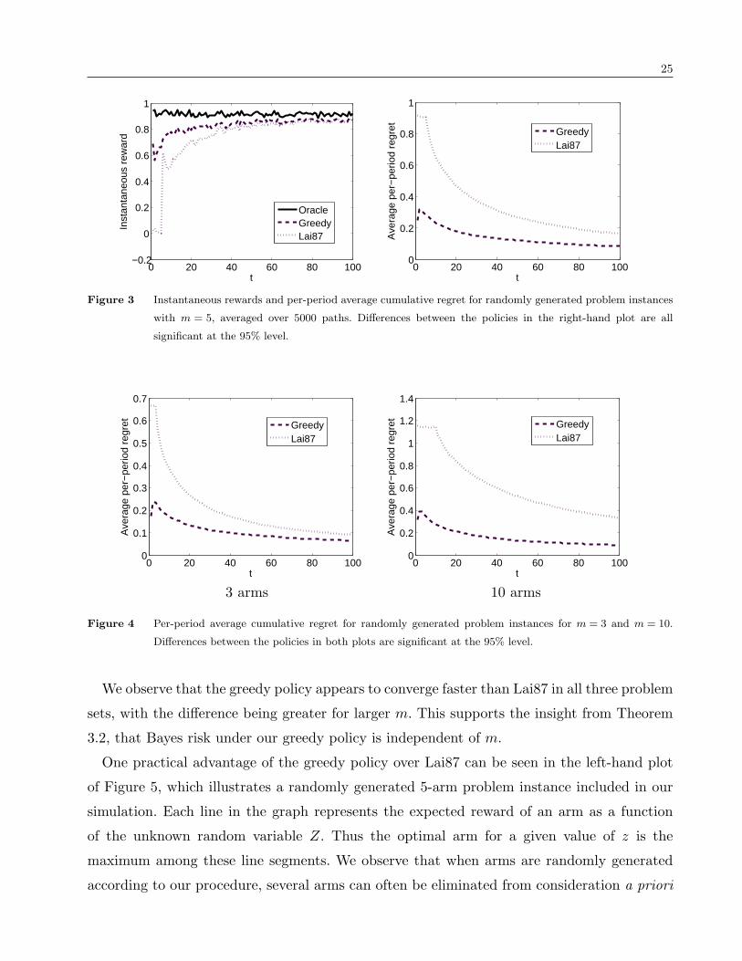
of z and always chooses the best arm. In Figure 3, we plot for the case m= 5, instantaneous

rewards X tJt

and per-period average cumulative regret,

1t

t∑s=1

(Xsoracle−Xs

Js),

both averaged over the 5000 paths. We include average cumulative regret plots for randomly-

generated 3- and 10-arm problems in Figure 4.

25

0 20 40 60 80 100−0.2

0

0.2

0.4

0.6

0.8

1

t

Inst

anta

neou

s re

war

d

OracleGreedyLai87

0 20 40 60 80 1000

0.2

0.4

0.6

0.8

1

t

Ave

rage

per

−pe

riod

regr

et

GreedyLai87

Figure 3 Instantaneous rewards and per-period average cumulative regret for randomly generated problem instances

with m = 5, averaged over 5000 paths. Differences between the policies in the right-hand plot are all

significant at the 95% level.

0 20 40 60 80 1000

0.1

0.2

0.3

0.4

0.5

0.6

0.7

t

Ave

rage

per

−pe

riod

regr

et

GreedyLai87

0 20 40 60 80 1000

0.2

0.4

0.6

0.8

1

1.2

1.4

t

Ave

rage

per

−pe

riod

regr

et

GreedyLai87

3 arms 10 arms

Figure 4 Per-period average cumulative regret for randomly generated problem instances for m = 3 and m = 10.

Differences between the policies in both plots are significant at the 95% level.

We observe that the greedy policy appears to converge faster than Lai87 in all three problem

sets, with the difference being greater for larger m. This supports the insight from Theorem

3.2, that Bayes risk under our greedy policy is independent of m.

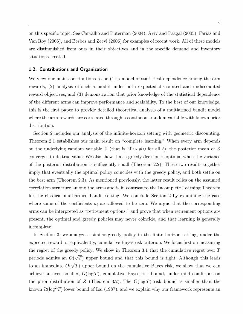
One practical advantage of the greedy policy over Lai87 can be seen in the left-hand plot

of Figure 5, which illustrates a randomly generated 5-arm problem instance included in our

simulation. Each line in the graph represents the expected reward of an arm as a function

of the unknown random variable Z. Thus the optimal arm for a given value of z is the

maximum among these line segments. We observe that when arms are randomly generated

according to our procedure, several arms can often be eliminated from consideration a priori

26

−2 −1 0 1 2−3

−2

−1

0

1

2

3

z

Exp

ecte

d R

ewar

ds

−2 −1 0 1 20

0.5

1

1.5

2

z

Exp

ecte

d R

ewar

ds

Figure 5 Mean reward of each arm as a function of z for a randomly generated problem (left) and a dynamic pricing

problem (right).

because they will never achieve the maximum for any realization of z. The greedy policy

will never choose such arms, though Lai87 may. On the other hand, recall that the greedy

policy’s performance is expected to depend on the constants u and u in Assumption 3.1,

which measure the magnitude and relative sizes of the slopes u`. (For example, the proof of

Theorem 3.1 indicates that the constants involved in the upper bound are proportional to

u/u.) For randomly selected problems, there will be instances in which the worst-case ratio

maxk,` |uk/u`| is large so that u/u is also large, resulting in less favorable performance bounds.

The second set of problem instances is inspired by the dynamic pricing problem formulated

in Section 1. We assume that the sales St` at time t under the price p` are of the form

St` = 2− p`b+ εt`, where b is normally distributed with mean µ = 1 and standard deviation

σ = 0.25. Thus, the revenue is Rt` = 2p`− p2

`b+ p`εt` = (2p`− p2

`µ)− σp`Z + p`εt`, where Z is a

standard normal random variable. We also assume that the errors εt` are normally distributed

with mean zero and variance 0.1. We set m = 5, corresponding to five prices: 0.75, 0.875,

1.0, 1.125, 1.25. The expected revenue as a function of z for each of the five arms/prices is

shown in the right-hand side plot of Figure 5. We see that in this instance, in contrast to

the randomly generated instance in the left-hand side plot, every arm is the optimal arm for

some realization of z.

We simulate 5000 runs, each involving a different value z, sampled from the standard normal

distribution, and we apply each one of our three policies: greedy, Lai87, and oracle. Figure 6

gives the instantaneous rewards and per-period average cumulative regret, both averaged over

the 5000 runs. Inspection of Figure 6 suggests that the greedy policy performs even better

relative to Lai87 in the dynamic pricing example than in the randomly generated instances.

27

0 20 40 60 80 1000.9

0.95

1

1.05

1.1

t

Inst

anta

neou

s re

war

d

OracleGreedyLai87

0 20 40 60 80 1000

0.02

0.04

0.06

0.08

0.1

0.12

t

Ave

rage

per

−pe

riod

regr

et

GreedyLai87

Figure 6 Per-period average cumulative regret for the dynamic pricing problem with 5 candidate prices. Differences

between the policies are significant at the 95% level.

Our greedy policy is clearly better able to take advantage of the inherent structure in this

problem.

5. Discussion and Future Research

We conclude by highlighting our main findings. We have removed the typical assumption made

when studying multiarmed bandit problems, that the arms are statistically independent, by

considering a specific statistical structure underlying the mean rewards of the different arms.

This setting has allowed us to demonstrate our main conjecture, namely, that one can take

advantage of known correlation structure and obtain better performance than if independence

were assumed. At the same time, we have specific results on the particular problem, with

univariate uncertainty, that we have considered. Within this setting, simple greedy policies

perform well, independent of the number of arms, for both discounted and undiscounted

objectives.

We believe that our paper opens the door to development of a comprehensive set of policies

that account for correlation structures in multiarmed bandit and other learning problems.

While correlated bandit arms are plausible in a variety of practical settings, many such

settings require a more general problem setup than we have considered here. Of particular

interest are correlated bandit policies for problems with multivariate uncertainty and with

more general correlation structures.

Acknowledgement

The authors would like to thank Hedibert Lopes, Gennady Samorodnitsky, Mike Todd, and

Robert Zeithammer for insightful discussions on problem formulations and analysis. The

28

first author thanks the University of Chicago Graduate School of Business for support. The

research of the second and third authors was supported in part by the National Science

Foundation through grants DMS-0732196 and ECCS-0701623, respectively.

A. Proof of Lemma 2.4

Proof: We will show that there exists a dominating function w : R×R+→R+ such that

sup(µ,θ)∈R×R+

|max` r(µ, θ, `)|w(µ, θ)

<∞,

and for each (µ, θ)∈R×R+,

max`

E [w (µ′(µ, θ, `), θ′(µ, θ, `))]≤w(µ, θ) +maxi |ui|

min|ui/γi| : ui 6= 0 .

The desired result then follows immediately from Theorem 1 in Lippman (1975).

Let η= max` |η`| and u= max` |u`|. For each (µ, θ)∈R×R, let

w(µ, θ) = η+ u

(|µ|+ 1√

θ

).

The first condition is clearly satisfied because for each state (µ, θ)∈R×R+ and arm `,

|r(µ, θ, `)|w(µ, θ)

≤ |η`|+ |u`||µ|w(µ, θ)

≤ 1.

To verify the second condition, note that if u` = 0, then µ′(µ, θ, `) = µ and θ′(µ, θ, `) = θ, with

probability one and the inequality is trivially satisfied. So, suppose that u` 6= 0. It follows

from the definition of w(·, ·) that

E [w (µ′(µ, θ, `), θ′(µ, θ, `))] = η+ uE |µ′(µ, θ, `)|+ u√θ′(µ, θ, `)

= η+ uE |µ′(µ, θ, `)|+ u√θ+u2

`/γ2`

≤ η+ uE |µ′(µ, θ, `)|+ u

min|ui/γi| : ui 6= 0

To establish the desired result, it thus suffices to show that E |µ′(µ, θ, `)| ≤ |µ|+ 1/√θ.

Since X t` = η` + u`Z +Et

`, Z ∼N (µ,1/θ), and Et` ∼N (0, γ2

` ), it follows that (X t` − η`)/u`

has the same distribution as µ+W√

1θ

+ γ2`

u2`, where W is an independent standard normal

random variable. It follows from the definition of µ′((µ, θ), `) that

E |µ′(µ, θ, `)|= E

∣∣∣∣∣∣µ+W(u2

`/γ2` )√

1θ

+ γ2`

u2`

θ+u2`/γ

2`

∣∣∣∣∣∣= E

∣∣∣∣∣µ+W

√u2`/γ

2`

θ2 + θu2`/γ

2`

∣∣∣∣∣≤ |µ|+ 1√θ,

29

where the second equality follows from the fact that

u2`

γ2`

√1θ

+ γ2`

u2`

θ+u2`/γ

2`

=u2`/γ

2`√

θ(u2`/γ

2` ) (θ+u2

`/γ2` )

=

√u2`/γ

2`

θ2 + θu2`/γ

2`

,

and the inequality follows from the facts that E|W |=√

2/π≤ 1 and√u2`/γ

2`

θ2 + θu2`/γ

2`

=1√θ

√u2`/γ

2`

θ+u2`/γ

2`

≤ 1√θ

B. Proof of Theorem 3.3

Proof: Fix some `, and let V be a random variable with the same distribution as Et`. For any

s∈R, let g`(s) = E[esV ]. Note that g`(0) = 1. Because of the exponential tails assumption on V ,

the function g`(s) is finite, and in fact infinitely differentiable, whenever |s|<λ. Furthermore,

its first derivative g′ satisfies g′`(0) = E[V ] = 0. Finally, its second derivative satisfies

g′′` (s) =d2

ds2E[esV ] = E

[V 2esV

].

(This step involves an interchange of differentiation and integration, which is known to be

legitimate in this context.)

It is well known that when a random variable |V | is stochastically dominated by another

random variable W , we have E[f(|V |)]≤ E[f(W )], for any nonnegative nondecreasing function

f . In our context, this implies that

g′′` (s) =E[V 2esV

]≤ E[V 2e|s|·|V |

]≤E[(U +x0)2e|s|(U+x0)].

The function on the right-hand side above is completely determined by b and x0. It is finite,

continuous, and bounded on the interval s ∈ [−b/2, b/2] by some constant f0 which only

depends on b and x0. It then follows that

g`(s)≤ 1 +f 2

0

2· s2, − b

2≤ s≤ b

2,

for all `.

We use the definition of Yt and the relation X tj = ηj +ujZ, to express Yt in the form

Yt =Z +1t

t∑τ=1

EτJτ

uJτ.

30

Let Dτ =EτJτ/uJτ . We will now use the standard Chernoff bound method to characterize the

tails of the distribution of the sum∑t

t=1Dτ .

Let Ft be the σ-field generated by Z and Ht, and note that Jt−1 is Ft−1-measurable. Let

also Qt(s) = E[esDt | Ft−1]. We observe that

Qt(s)≤ max`=1,...,m

E[esEt`/u`]≤ 1 +

f 20

2u2· s2 = 1 + f3s

2, − b2≤ s≤ b

2, (5)

where the last equality is taken as the definition of f3.

Now, note that

E

[es(D1+···+Dt)

Q1(s) · · ·Qt(s)

∣∣∣ Ft−1

]=

es(D1+···+Dt−1)

Q1(s) · · ·Qt−1(s).

It then follows (for example, by taking expectations and using induction) that

E

[es(D1+···+Dt)

Q1(s) · · ·Qt(s)

∣∣∣ Z]= 1.

Using the bound from Eq. (5), we obtain

E[es(D1+···+Dt) |Z]≤ (1 + f3s2)t, − b

2≤ s≤ b

2.

Fix some t≥ 1, a> 0, and z ∈R. We have, for any s∈ [−b/s, b/2],

Pr(Yt− z > a |Z = z) = Pr(D1 + · · ·+Dt > ta |Z = z)

≤ e−staE[es(D1+···+Dt) |Z = z]

≤ e−sta(1 + f3s2)t

= e−staet ln(1+f3s2)

≤ e−staef3s2t. (6)

Suppose first that a satisfies a≥ bf3. By applying inequality Eq. (6) with s= b/2, we obtain

Pr(Yt− z > a |Z = z)≤ e−(tba/2)+(tf3b2/4) ≤ e−(tba/2)+(tba/4) = e−tba/4.

Suppose next that a satisfies a < bf3. By applying inequality Eq. (6) with s= a/(2f3)< b/2,

we obtain

Pr(Yt− z > a |Z = z)≤ e−(ta2/2f3)+(tf3a2/4f23 ) = e−ta

2/4f3.

Since for every positive value of a one of the above two bounds applies, we have

Pr(Yt− z > a |Z = z)≤ e−f1at + e−f1a2t,

where f1 = minb/4,1/4f3. The expression Pr(Yt − z > a | Z = z) can be bounded by a

symmetrical argument, and the proof of the tail bounds is complete.

The bounds on the moments of Yt follow by applying the formula E[X2] = 2∫∞

0xPr(X >

x)dx− 2∫ 0

−∞ xPr(X <x)dx, and some straightforward algebra.

31

C. Proof of Proposition 3.4

Proof: We fix some ε > 0. Recall that the maximum expected reward function g is defined

by g(z) = max` η` +u`z, where the maximization ranges over all arms in our collection.

Consider a problem with an infinite number of arms where the function g(·) is given by:

g(z) =

−z, if z < 0,z+ z1+ε

1+ε, if 0≤ z ≤ 1,

2z− ε1+ε, if 1< z

Note that the function g is convex and continuous, and its derivative is given by:

g′(z) =

−1, if z < 0,1 + zε, if 0≤ z ≤ 1,2, if 1< z

In particular, u= 1 and u= 2. We assume that for each a ∈R, the error Eta associated with

arm a∈R is normally distributed with mean zero and variance (g′(a))2; then Assumption 3.1

is satisfied. We will consider the case where z = 0 and show that the cumulative regret over

T periods is Ω(T 0.5−ε).

Consider our estimate Yt of z at the end of period t, which is normal with zero mean and

variance 1/t. In particular,√tYt is a standard normal random variable. If Yt < 0, then the

arm chosen in period t+1 is the best one, and the instantaneous regret in that period is zero.

On the other hand, if 0≤ Yt ≤ 1, then the arm a chosen in period t+ 1 will be for which the

line ηa +uaz is the tangent of the function g(·) at Yt, given by

ht+1(x) = g′ (Yt)x−εY 1+ε

t

1 + ε,

where the choice of the intercept is chosen so that ht+1 (Yt) = g (Yt). If Yt > 1, the instantaneous

regret can only be worse than if 0≤ Yt ≤ 1. This implies that the instantaneous regret incurred

in period t+ 1 satisfies

r (z,Yt)≥1l (0<Yt < 1)g(z)−ht+1(z)= 1l (0<Yt < 1)εY 1+ε

t

1 + ε≥ 1l

(0<Yt <

1√t

)εY 1+ε

t

1 + ε,

where the equality follows from the fact that z = 0. Therefore, the instantaneous regret

incurred in period t+ 1 is lower bounded by

E [r (z,Yt) |Z = z] ≥ ε

1 + εE

[1l(

0<Yt <1√t

)·Y 1+ε

t |Z = z

]=

ε

(1 + ε) t(1+ε)/2E

[1l(

0<Yt <1√t

)·(√

tYt

)1+ε

|Z = z

]=

ε

(1 + ε) t(1+ε)/2E[1l (0<W < 1) ·W 1+ε

],

32

where W is a standard normal random variable. Therefore, the cumulative regret over T

periods can be lower bounded as follows:

Regret(z,T,Greedy) ≥T−1∑t=1

E [r (z,Yt) |Z = z]

=εE [1l (0<W < 1) ·W 1+ε]

1 + ε

T−1∑t=1

1t(1+ε)/2

= Ω(T (1−ε)/2),

where the last inequality follows, for example, by approximating the sum by an integral.

References

Agrawal, R. 1996. Sample mean based index policies with O(log n) regret for the multi-armed bandit problem.

Adv. Appl. Prob. 27 1054–1078.

Agrawal, R., T. Domosthenis, V. Anantharam. 1989. Asymptotically efficient adaptive allocation schemes. IEEE

T. Automat. Contr. 34(12) 1249–1259.

Auer, P., N. Cesa-Bianchi, P. Fischer. 2002a. Finite-time analysis of the multiarmed bandit problem. Mach.

Learn. 47 235–256.

Auer, P., N. Cesa-Bianchi, Y. Freund, P. Fischer. 2002b. The nonstochastic multiarmed bandit problem. SIAM

J. Comput. 32(1) 48–77.

Aviv, Y., A. Pazgal. 2005. Dynamic pricing of short life-cycle products through active learning. Working paper,

Olin School of Business, Washington University.

Banks, J. S., R. K. Sundaram. 1992. Denumerable-armed bandits. Econometrica 60 1071–1096.

Berry, D., B. Fristedt. 1985. Bandit Problems: Sequential Allocation of Experiments. Chapman and Hall,

London.

Bertsimas, D., J. Nino-Mora. 1996. Conservation laws, extended polymatroids and multi-armed bandit problems.

Math. Oper. Res. 21 257–306.

Besbes, O., A. Zeevi. 2006. Dynamic pricing without knowing the demand function: Risk bounds and near-

optimal algorithms. Working paper, Columbia University.

Brezzi, M., T. L. Lai. 2000. Incomplete learning from endogenous data in dynamic allocation. Econometrica

68(6) 1511–1516.

Carvalho, A., M. Puterman. 2004. How should a manager set prices when the demand function is unknown?

Working paper, University of British Columbia.

Dani, V., T. Hayes. 2006. Robbing the bandit: Less regret in online geometric optimization against an adaptive

adversary. Proceedings of the 17th Annual ACM-SIAM Symposium on Discrete Algorithms.

Durrett, R. 1996. Probability: Theory and Examples. Duxbury Press, Belmont.

33

Farias, V. F., B. Van Roy. 2006. Dynamic pricing with a prior on market response. Working paper, Stanford

University.

Feldman, D. 1962. Contributions to the “two-armed bandit” problem. Ann. Math. Stat. 33 847–856.

Flaxman, A., A. Kalai, H. B. McMahan. 2005. Online convex optimization in the bandit setting: Gradient descent

without a gradient. Proceedings of the 16th Annual ACM-SIAM Symposium on Discrete Algorithms.

Foster, D. P., R. Vohra. 1999. Regret in the on-line decision problem. Games and Economic Behavior 29 7–35.

Frostig, E., G. Weiss. 1999. Four proofs of Gittins’ multiarmed bandit theorem. Working paper, University of

Haifa.

Ginebra, J., M. K. Clayton. 1995. Response surface bandits. J. Roy. Stat. Soc. B 57(4) 771–784.

Gittins, J., D. M. Jones. 1974. A dynamic allocation index for the sequential design of experiments. J. Gani,

ed., Progress in Statistics. North-Holland, Amsterdam, 241–266.

Keener, R. 1985. Further contributions to the “two-armed bandit” problem. Ann. Stat. 13(1) 418–422.

Kleinberg, R. 2005. Nearly tight bounds fro the continuum-armed bandit problem. Advances in Neural Infor-

mation Processing Systems 17 .

Kleinberg, R. 2008. Online linear optimization and adaptive routing. J. Computer and System Sciences 74(1)

97–114. Extended abstract appeared in Proceedings of the 36th ACM Symposium on Theory of Computing

(STOC 2004).

Lai, T. L. 1987. Adaptive treatment allocation and the multi-armed bandit problem. Ann. Stat. 15(3) 1091–1114.

Lai, T. L., H. Robbins. 1978. Adaptive design in regression and control. Proc. Natl. Acad. Sci. 75(2) 586–587.

Lai, T. L., H. Robbins. 1985. Asymptotically efficient adaptive allocation rules. Adv. Appl. Math. 6 4–22.

Lippman, S. A. 1975. On dynamic programming with unbounded rewards. Manage. Sci. 21(11) 1225–1233.

McMahan, H. B., A. Blum. 2004. Online geometric optimization in the bandit setting against an adaptive

adversary. Proceedings of the 17th Annual Conference on Learning Theory .

Pandey, S., D. Chakrabarti, D. Agrawal. 2007. Multi-armed bandit problems with dependent arms. Proceedings

of the 24th International Conference on Machine Learning .

Pressman, E. L., I. N. Sonin. 1990. Sequential Control With Incomplete Information. Academic Press, London.

Robbins, H. 1952. Some aspects of the sequential design of experiments. Bull. Amer. Math. Soc. 58 527–535.

Rothschild, M. 1974. A two-armed bandit theory of market pricing. Journal of Economic Theory 9 185–202.

Shaked, M., J. G. Shanthikumar. 2007. Stochastic Orders. Springer, New York.

Tewari, A., P. L. Bartlett. 2008. Optimistic linear programming gives logarithmic regret for irreducible mdps.

Advances in Neural Information Processing Systems 20 .

Thompson, W. R. 1933. On the likelihood that one unknown probability exceeds another in view of the evidence

of two samples. Biometrika 25 285–294.

34

Tsitsiklis, J. N. 1994. A short proof of the Gittins index theorem. The Annals of Applied Probability 4(1)

194–199.

Weber, R. R. 1992. On the Gittins index for multiarmed bandits. Ann. Prob. 2 1024–1033.

Whittle, P. 1980. Multi-armed bandits and the Gittins index. J. Royal Stat. Soc. B 42 143–149.