Physica D ( ) –

Contents lists available at ScienceDirect

Physica D

journal homepage: www.elsevier.com/locate/physd

A Stokesian viscoelastic flow: Transition to oscillations and mixingBecca Thomases a,∗, Michael Shelley b, Jean-Luc Thiffeault ca Department of Mathematics, University of California, Davis, CA 95616, United Statesb Courant Institute of Mathematical Sciences, New York University, New York City, NY 10012, United Statesc Department of Mathematics, University of Wisconsin Madison, WI 53706, United States

a r t i c l e i n f o

Article history:Available online xxxx

Keywords:ViscoelasticityInstabilityMixingMicrofluidics

a b s t r a c t

To understand observations of low Reynolds number mixing and flow transitions in viscoelastic fluids,we study numerically the dynamics of the Oldroyd-B viscoelastic fluid model. The fluid is driven by asimple time-independent forcing that, in the absence of viscoelastic stresses, creates a cellular flow withextensional stagnation points. We find that at O(1) Weissenberg number, these flows lose their slavingto the forcing geometry of the background force, become oscillatory with multiple frequencies, and showcontinual formation and destruction of small-scale vortices. This drives flow mixing, the details of whichwe closely examine. These new flow states are dominated by a single-quadrant vortex, which may bestationary or cycle persistently from cell to cell.

© 2011 Elsevier B.V. All rights reserved.

1. Introduction

In the past several years, it has come to be appreciated thatin low Reynolds number flow the nonlinearities provided bynon-Newtonian stresses of a complex fluid can provide richdynamical behaviors more commonly associated with highReynolds number Newtonian flow. For example, experimentsby Steinberg and collaborators have shown that dilute polymersuspensions being sheared in simple flow geometries can exhibithighly time-dependent dynamics and efficient mixing [1–3]. Thecorresponding experiments using Newtonian fluids do not – andindeed cannot – show such nontrivial dynamics. One importantconstraint on the dynamics of a Stokesian Newtonian fluid isreversibility [4], which is lost when the fluid is viscoelastic [5,6].

Both mixing and irreversibility are complex phenomena buteven the understanding of elastic instabilities in viscoelastic fluidsis incomplete. Elastic instabilities in low Reynolds number fluids,where inertia is negligible, have been studied extensively for sometime; see [7–14]. Elastic instabilities are observed at low ormodestflow rates where inertial forces are negligible but elastic forces arestrong, and have been linked to the creation of secondary vortexflows [15] and increased flow resistance [16].

Extensional flows, such as the flow in a four-roll mill or flowin a cross-channel, can be more effective in locally stretchingand aligning polymers than a standard shear flow [17]. Asthe macroscopic flow depends on the microscopically generated

∗ Corresponding author. Tel.: +1 5305542988; fax: +1 5307526635.E-mail address: thomases@math.ucdavis.edu (B. Thomases).

stresses, a flow in an extensional geometry may exhibit aninstability more readily than a flow in a shearing geometry. Thismay be due to the fact that a shear flow can be decomposedinto an extensional flow and a rotational flow and the vorticityin the fluid tends to rotate the fluid microstructure away fromthe principal axes of stretching [18,13]. Experiments have shownthat polymer molecules are strongly stretched as they pass nearextensional points in amicro-channel cross flow [19,20]. Schroederet al. [19] visualized single-molecule stretching and bistability atstagnation points. In the work of Arratia et al. [20], molecularstretching is inferred and two flow instabilities, dependent onthe flow strain rate, are demonstrated. After the onset of thefirst instability, the flow becomes deformed and asymmetric butremains steady; at higher strain rates the velocity field fluctuatesin time and can produce mixing. The first transition appears to bea forward bifurcation to a bistable steady state; see also [21,22].In [23], (henceforth TS2009) these instabilities are demonstratednumerically for a 2D periodic flow, and these results are discussedin greater detail here. Xi and Graham [24] also found numericallyan oscillatory instability for sufficiently largeWeissenberg numberin an extensional flow geometry, and they suggest a possiblemechanism for the instability due to the concentration of stressnear the extensional point in the flow. In [25], Berti et al. shownumerically that flows with a 2D periodic shearing force can giverise to non-stationary dynamics.

In this paper, we study computationally a viscoelastic fluidin an extensional flow. As our flow model, we use the Oldroyd-B equations with polymer stress diffusion in the zero Reynoldsnumber (Stokes) limit. The Stokes–Oldroyd-B model is attractiveas it arises from a simple conception of the microscopic origin ofviscoelasticity [26,27]. The bulk fluid is composed of a Newtonian

0167-2789/$ – see front matter© 2011 Elsevier B.V. All rights reserved.doi:10.1016/j.physd.2011.06.011

2 B. Thomases et al. / Physica D ( ) –

(Stokesian) solvent with a dilute concentration of immersedpolymer chains, themselves modeled as Hookean springs. Thepolymer stress is proportional to the second moment of theconfiguration distribution function. One consequence of modelingthe response of a polymer coil as a linear Hookean spring is thatthe Oldroyd-B equations put no limit on the deformed lengthof a stretched coil. This yields unphysical infinite viscosities atfinite strain rates for viscometric straining flows [27]. In [28] thisdefect in the model was linked to the exponential growth of thepolymer stress at extensional stagnation points in the flow; seealso [29–32].

As part of the calibration of our model we compare it withthe standard Stokes–Oldroyd-B model and the FENE-P model(a modification of the Oldroyd-B model which enforces a finitepolymer extension length) for 2D periodic extensional flows (seeAppendix B). We show that adding a small amount of polymerstress diffusion yields structures qualitatively similar to FENE-Pwhile maintaining a bounded and smooth polymer stress field.This diffusion term is not added without physical justification,as some polymer stress diffusion can be justified from kinetictheory [26] and there aremany other proposedmodels which seekto incorporate it; see for example [33–35].

In a previous study [28] (henceforth TS2007) Thomases andShelley studied the standard Stokes–Oldroyd-B model in twodimensions. The relevant results from this study will be reviewedin Section 2. Here we add perturbations to the flows studiedin TS2007 and look at the dynamics that are introduced. Ourmain observation is that for sufficiently largeWeissenberg numberthe symmetric solutions obtained in TS2007 are not stableto asymmetric perturbations in the initial data. Rather, theseperturbations induce a symmetry-breaking transition which willlead to asymmetric states that are qualitatively different incharacter from the symmetric solutions found in TS2007 and fromsolutions at small Weissenberg number.

Furthermore it is shown that this transition to an asymmetricstate leads to enhanced mixing in the fluid across large regionsof the flow domain. For low Weissenberg number flows the four-roll mill flow topology is preserved and hence fluid particles neardistinct rollers do not mix. However, when the flow transitions tothe asymmetric state and then to a state with higher-frequencytime-dependent fluctuations there can be significant mixing.

In Section 2, the Stokes–Oldroyd-B equations with diffusionare described along with some basic properties. The numericalmethod used in the simulations is described in Appendix A, andthe choice and calibration of our model is discussed in Appendix B.We discuss the transitions in Section 3. In Section 3.1 we provide adetailed look at the first symmetry-breaking transition. Section 3.2gives results from perturbing the flow with initial data of randomstructure. There is a second transition which occurs in the flow(at higherWeissenberg number) andwe conjecture an explanationfor this second transition in Section 3.3. Section 4 is devoted to adiscussion of mixing in the fluid, including both demonstrationsof the phenomena and measures to quantify the level of mixing.We discuss the effective diffusion induced by the polymer stress inSection 4.2 and compute Lyapunov exponents in Section 4.3. Ourconclusions and further directions are discussed in Section 5.

2. Background

The 2d Stokes–Oldroyd-B system with polymer stress diffusionis given in dimensionless form by:

−∇p + u = −β∇ · S + f, ∇ · u = 0, (1)

S∇+ (W i)−1(S − I) = νpS, (2)

where the upper convected time derivative, S∇ , is defined by

S∇≡

∂S∂t

+ u · ∇S − (∇u S + S ∇uT ). (3)

The polymer stress, S, is a symmetric positive definite 2-tensorand its trace (S11 + S22) represents the mean-squared distensionof polymer coils. The Weissenberg number is given by W i = τp/τf ,with τp the polymer relaxation time and τf a typical time-scale ofthe fluid flow. Here, our external force, f, is used to drive the flow,and its dimensional scale F is used to set the flow time-scale asτf = µ/ρLF , where µ is the solvent viscosity, ρ the fluid density,and L the system size. This sets the dimensionless force, and thetime-scale of transport, to be order one. With the particular choicehere for f, τ−1

f is also the strain rate of extensional stagnationpoints in the induced Newtonian flow, which explains our use ofthe Weissenberg number rather than the Deborah number for thisdiscussion.

The parameter β = Gτf /µ measures the relative contributionof the polymer stress to the momentum balance, where G isthe isotropic stress induced by the polymer field in the absenceof flow. The parameter νp controls the polymer stress diffusion.Stress diffusion can arise when including the effect of center ofmass diffusion of polymer coils [36]. Here it is added to controlpolymer stress gradient growth as Eqs. (1)–(2) otherwise lack ascale-dependent dissipation (see also [33–35] for other modelsincorporating stress diffusion). In the following simulations wefix νp = 10−3; the calibration of this parameter is discussed inAppendix B.

The quantity β · W i is the ratio of the polymer viscosity tosolvent viscosity, so that given a particular working fluid the ratiois fixed independent of experimental conditions. As a useful pointof comparison, from the work of Arratia et al. [20] the solutionviscosity is 1.2 Pa s, while the solvent (97% glycerol/water) is 0.8 Pas, yielding β · W i = (1.2 − 0.8)/0.8 = 0.5. We keep the productβ · W i = 0.5 in our simulations.

The Stokes–Oldroyd-B equations with polymer stress diffusionalso have a relative strain energy for the distension of the polymerfield:

E(t) =12

Ω

trace (S − I) dx, (4)

which satisfies

E + W i−1E = −D + W, (5)

where

D = β−1

|∇u|2 dx

is the rate of viscous dissipation and

W = −β−1

f · u dx

is the power input by the forcing. Note that for fixed β , E(t) willdecay (for f ≡ 0) even in the limit of infinite W i owing to theviscous response of the Newtonian solvent.

The standard Stokes–Oldroyd-B equations are given by Eqs.(1)–(2) with νp = 0. In this case, the Newtonian Stokes equationsare recovered in the limit W i → 0, in which case the polymerstress is uniform and isotropic. In TS2007 the 2D Stokes–Oldroyd-B equations were simulated on a 2π-periodic domain, [−π, π]

2,with a steady background force of the form

f =

2 sin x cos y

−2 cos x sin y

. (6)

In a Newtonian Stokes flow with doubly periodic boundaryconditions this yields the velocity field u = −

12 f, which is a four-

roll mill flow with counter-rotating vortices of equal magnitude.

B. Thomases et al. / Physica D ( ) – 3

2.05

2.1

2.15

2.2

2.25

2.3

2.35

–1

–0.5

0

0.5

1

–1

–0.5

0

0.5

1

2.22.42.62.833.23.43.63.844.2

50

100

150

200

250

–0.8–0.6–0.4–0.200.20.40.60.8

Wi= 0.3 Wi= 0.6 Wi= 5.0a b c

d e f

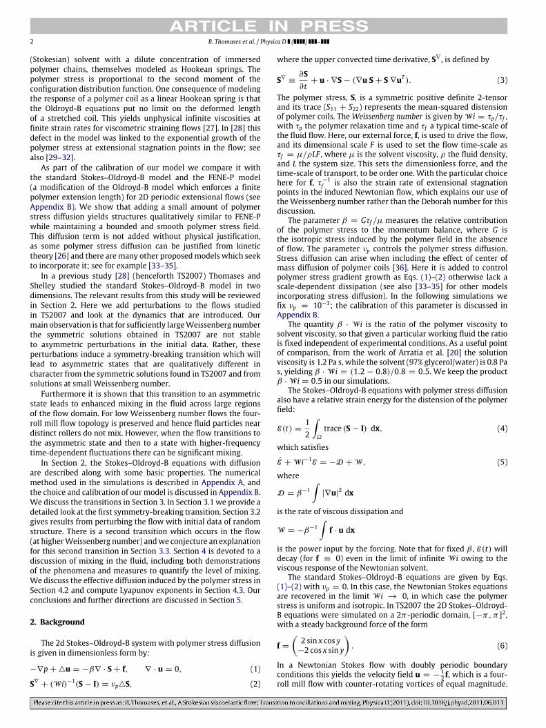
Fig. 1. Contour plots of components of velocity and polymer stress evolving from Stokes–Oldroyd-B equations without polymer stress diffusion and isotropic initial data att = 6. (a)–(c) Vorticity for W i = 0.3, 0.6, and 5 respectively. (d)–(f) tr S for W i = 0.3, 0.6, and 5 respectively. From TS2007 with permission.

This forcing fixes an extensional stagnation point at the origin(and (±π, 0), (0, ±π), and (±π, ±π)). The stagnation points aremaintained dynamically if the flow is not perturbed and the initialstress is isotropic, S(0) = I.

In TS2007 it was observed that for small Weissenberg number,W i < 0.5, the polymer stress reaches a smooth steady state rapidlyand the velocity field remains slaved to the background force;see Fig. 1(a). For 0.5 . W i . 1 the polymer stress convergesexponentially in time to a solution which has a singularity inthe first derivative, a cusp; see Fig. 1(e). However, the vorticityfield is qualitatively unchanged by this emerging singularity; seeFig. 1(b). However, for sufficiently large Weissenberg number,W i & 1, the polymer stress diverges exponentially in time; seeFig. 1(f). The vorticity field is shown in Fig. 1(c) where we see thatsmaller oppositely signed vortices emerge along the incoming andoutgoing streamlines of the extensional points in the flow.

The singular behavior in the polymer stress, and the criticalvalues for the transitions, was confirmed by constructing adynamical local solution which agrees very well with thesimulations near the extensional point in the flow; see also [37,32].For W i & 1, tr S concentrates on sets of exponentially decreasingmeasure along the streamlines associated with the extensionalstagnation point, which may in part be why the velocity fieldappears to reach a steady state where the polymer stress fieldis diverging exponentially. With isotropic initial data for S, thepolymer stress and velocity field remain symmetric, in particular,the S22 field is a rotation and translation of the S11 field, tr S has4-fold symmetry, and each component of the polymer stress andthe vorticity have 2-fold symmetry.

3. Instabilities

3.1. Symmetry breaking

With isotropic initial data, S(0) = I, Eqs. (1)–(2) are simulatedin a 2D periodic box [−π, π]

2 with steady background force fgiven by (6). The system is solved by a pseudo-spectral method(see Appendix A for details). With n2

= 2562 grid-points, thehigh-wavenumber part of the spatial Fourier spectrum isO(10−12)throughout the simulations, and doubling the spatial resolutiondoes not change the observed dynamics. For W i ≤ 10 and νp =

10−3 solutions converge to steady states which are reminiscent

of the solutions found in TS2007. The main difference is that thepolymer stress is cut off by diffusion, and now saturates, withS remaining smooth and bounded. Other features seen in thesolutions from TS2007 (Fig. 1) are quite similar: tr S concentratesin symmetric ‘‘stress islands’’ along the outgoing streamlines ofthe flow. There is a coil-stretch transition which occurs aroundW i ≈ 1, beyond which tr S grows rapidly initially and additionaloppositely signed vortices arise along the incoming and outgoingstreamlines of extensional points in the flow, similar to those seenin Fig. 1(c) and (f).

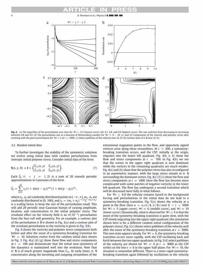
To investigate the stability of these steady symmetric solutionswe add small perturbations to symmetric steady solutions whichhave evolved from S(0) = I. We consider a state to be ‘‘converged’’if max |S(t + 1) − S(t)| < 10−7. For the symmetric solutionsS11(x, y) is an even function of both x and y, so we introducea small perturbation to the first odd Fourier mode in the yvariable. The perturbation is O(.05), and does not depend on theWeissenberg number or the extra stress diffusion. We focus on thefirst symmetry-breaking transition which occurs for W i ≈ 4.8.Here we try to pinpoint the critical value of W i beyond whichthis symmetry breaking will occur and the rate at which itoccurs. We plot the size of the perturbation in this mode as afunction of time for each W i. Fig. 2(a) shows the logarithm of theperturbation for 0 < t < 200 for W i = 4.5, 4.6, 4.7, 4.8, and 4.9,while Fig. 2(b) shows the computed perturbation decay/growthrate. The transition from a decaying perturbation to a growingperturbation occurs between W i = 4.8 and W i = 4.9. There doesappear to be a local maximum in the growth rate near W i = 9.

Fig. 2(c) and (d) show components of the flow for W i = 5 att = 1000, as a result of this initial perturbation. Fig. 2(c) showspathlines of the velocity field at a fixed time for somepoints locatednear the origin (the dot and dotted lines are at the origin, x = 0,and y = 0) and we see that the perturbation has caused the centralstagnation point (CSP) to move into the upper half-plane, losingeven symmetry in y. Similarly, Fig. 2(d) shows contour lines of tr Sin the perturbed state, again having lost symmetry in the y-variable(the dotted lines are at x = 0 and y = 0). When the perturbationsize is doubled or halved, the perturbation decay/growth rate doesnot change, nor does it change when the perturbation is made in adifferent Fourier mode. The transition W i also does not depend onthe size or location of the perturbation. When the perturbation isintroduced in the x-variable, the CSPmoves into the left half-plane,along the line x = 0, losing symmetry in this variable.

4 B. Thomases et al. / Physica D ( ) –

a b

c d

Fig. 2. (a) The logarithm of the perturbation over time for W i = 4.5 (lowest curve), 4.6, 4.7, 4.8, and 4.9 (highest curve). The rate switches from decreasing to increasingbetween 4.8 and 4.9. (b) The perturbation rate as a function of Weissenberg number for W i ≈ 4 − 10. (c) and (d) Components of the velocity and polymer stress afterevolving with the given perturbation for W i = 5 at t = 1000. (c) Select pathlines of the velocity near (0, 0) (d) Contour lines of tr S near (0, 0)..

3.2. Random initial data

To further investigate the stability of the symmetric solutionswe evolve using initial data with random perturbations fromisotropic initial polymer stress. Consider initial data of the form

S(x, y, 0) = I +S11(x, y) S12(x, y)S12(x, y) S22(x, y)

. (7)

Each Sij (i < j = 1, 2) is a sum of 20 smooth periodicapproximations to Gaussians of the form

Sij =

20k=1

ck(1 + sin(x − xk))mk(1 + sin(y − yk))nk ,

where xk, yk are randomly distributed points in [−π, π],mk, nk arerandomly distributed in [0, 100], and ck = (mk + nk)

−1/22−(mk+nk)

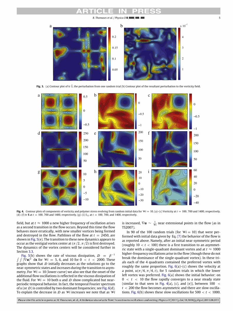
is a scaling factor to keep the size of the perturbation small. Thiswill add 20 periodic near-Gaussian bumps of varying amplitude,location, and concentration to the initial polymer stress. Theresultant effect on the velocity field is an O(10−3) perturbationfrom the four-roll mill geometry. For an example, a contour plotof the perturbation tr S is shown in Fig. 3(a) and a contour plot ofthe resultant perturbation to the vorticity is given in Fig. 3(b).

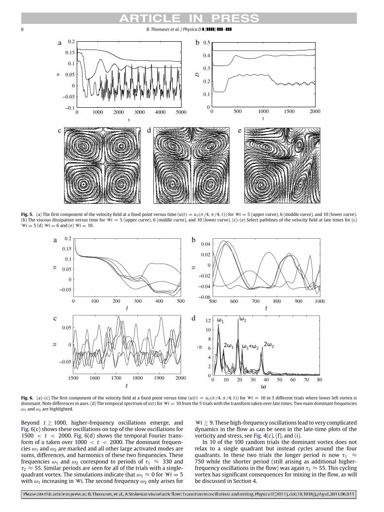
Fig. 4 shows the vorticity and polymer stress components bothbefore and after the onset of a symmetry-breaking transition forW i = 10. Solutions evolve from the random initial data shownin Fig. 3. Fig. 4(a) (d) (g) show these flow and stress componentsat t = 100 and demonstrate that the initial near-symmetry ofthe dynamics is maintained well into the evolution. Note thattr S is of much greater magnitude than S12. At early times, tr Sconcentrates along the incoming and outgoing streamlines of the

extensional stagnation points in the flow, and oppositely signedvortices arise along these streamlines. At t ≈ 200, a symmetry-breaking transition occurs, and the CSP, initially at the origin,migrates into the lower left quadrant. Fig. 4(b, e, h) show theflow and stress components at t = 700. In Fig. 4(b) we seethat the vortex in the upper right quadrant is now dominantwhile the vortices in the remaining quadrants are much weaker.Fig. 4(e) and (h) show that the polymer stress has also reconfiguredin an asymmetric manner, with the large stress islands in tr Ssurrounding the dominant vortex. Fig. 4(c) (f) (i) show the flow andstress components at t = 1400. Here the flow has become morecomplicated with some patches of negative vorticity in the lowerleft quadrant. The flow has undergone a second transition whichwill be discussed more fully in what follows.

For W i . 4.8 the velocity remains slaved to the backgroundforcing and perturbations in the initial data do not lead to asymmetry-breaking transition. Fig. 5(a) shows the velocity at apoint in the flow (here u = u1(π/4, π/4)) over 0 < t < 5000for W i = 5 (upper curve), W i = 6 (middle curve), and W i = 10(lower curve). Dynamically, what is observed forW i = 5 is that theonset of the symmetry-breaking transition is quite slow, with theCSP slowlymigrating into the upper right quadrant (the simulationshown here is for a different random initial configuration of thepolymer stress). Fig. 5(c) shows select pathlines of the velocitywellafter the onset of the symmetry-breaking transition at t = 3000.This new state appears steady. ForW i = 6, the symmetry-breakingtransition occurs more rapidly, with the CSP oscillating back andforth between the twoupper quadrants. In Fig. 5(d) select pathlinesof the velocity are shown for W i = 6 at t = 4000 as the CSPsettles on the line x = 0 in the upper half-plane. For W i = 10, thesituation is somewhat different. There is a more rapid symmetry-breaking transition again followed by oscillations in the velocity

B. Thomases et al. / Physica D ( ) – 5

a b

Fig. 3. (a) Contour plot of tr S, the perturbation from one random trial (b) Contour plot of the resultant perturbation to the vorticity field.

a b c

d e f

g h i

Fig. 4. Contour plots of components of vorticity and polymer stress evolving from random initial data for W i = 10. (a)–(c) Vorticity at t = 100, 700 and 1400, respectively.(d)–(f) tr S at t = 100, 700 and 1400, respectively. (g)–(i) S12 at t = 100, 700, and 1400, respectively.

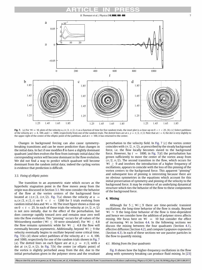
field, but at t ≈ 1000 a new higher frequency of oscillation arisesas a second transition in the flow occurs. Beyond this time the flowbehaves more erratically, with new smaller vortices being formedand destroyed in the flow. Pathlines of the flow at t = 2450, areshown in Fig. 5(e). The transition to these newdynamics appears tooccur as the vestigial vortex center at (π/2, π/2) is first destroyed.The dynamics of the vortex centers will be considered further inSection 3.3.

Fig. 5(b) shows the rate of viscous dissipation, D = β−1 |∇u|

2 dx for W i = 5, 6, and 10 for 0 < t < 2000. Thesegraphs show that D initially decreases as the solutions go to thenear-symmetric states and increases during the transition to asym-metry. For W i = 10 (lower curve) we also see that the onset of theadditional flow oscillations is reflected in the viscous dissipation ofthe fluid. For W i = 10 both u and D show complicated but near-periodic temporal behavior. In fact, the temporal Fourier spectrumof u (orD) is controlled by two dominant frequencies; see Fig. 6(d).To explain the decrease in D as W i increases we note that as W i

is increased, ∇u ∼1

W i near extensional points in the flow (as inTS2007).

In 90 of the 100 random trials (for W i = 10) that were per-formedwith initial data given by Eq. (7) the behavior of the flow isas reported above. Namely, after an initial near-symmetric period(roughly 10 < t < 100) there is a first transition to an asymmet-ric state with a single-quadrant dominant vortex and at t ≈ 1000higher-frequency oscillations arise in the flow (though these donotbreak the dominance of the single-quadrant vortex). In these tri-als each of the 4 quadrants contained the preferred vortex withroughly the same proportion. Fig. 6(a)–(c) shows the velocity ata point, u(π/4, π/4, t), for 5 random trials in which the lowerleft vortex was preferred. Fig. 6(a) shows the initial behavior: on0 < t < 10 the flow rapidly converges to a near steady state(similar to that seen in Fig. 4(a), (c), and (e)), between 100 <

t < 200 the flow becomes asymmetric and there are slow oscilla-tions. Fig. 6(b) shows these slow oscillations for 500 < t < 1000.

6 B. Thomases et al. / Physica D ( ) –

a b

c d e

Fig. 5. (a) The first component of the velocity field at a fixed point versus time (u(t) = u1(π/4, π/4, t)) for W i = 5 (upper curve), 6 (middle curve), and 10 (lower curve).(b) The viscous dissipation versus time for W i = 5 (upper curve), 6 (middle curve), and 10 (lower curve). (c)–(e) Select pathlines of the velocity field at late times for (c)W i = 5 (d) W i = 6 and (e) W i = 10.

a b

c d

Fig. 6. (a)–(c) The first component of the velocity field at a fixed point versus time (u(t) = u1(π/4, π/4, t)) for W i = 10 in 5 different trials where lower left vortex isdominant. Note differences in axes. (d) The temporal spectrum of u(t) forW i = 10 from the 5 trials with the transform taken over late times. Twomain dominant frequenciesω1 and ω2 are highlighted.

Beyond t & 1000, higher-frequency oscillations emerge, andFig. 6(c) shows these oscillations on top of the slow oscillations for1500 < t < 2000. Fig. 6(d) shows the temporal Fourier trans-form of u taken over 1000 < t < 2000. The dominant frequen-cies ω1 and ω2 are marked and all other large activated modes aresums, differences, and harmonics of these two frequencies. Thesefrequencies ω1 and ω2 correspond to periods of τ1 ≈ 330 andτ2 ≈ 55. Similar periods are seen for all of the trials with a single-quadrant vortex. The simulations indicate that ω1 ≈ 0 for W i = 5with ω1 increasing in W i. The second frequency ω2 only arises for

W i & 9. These high-frequency oscillations lead to very complicateddynamics in the flow as can be seen in the late-time plots of thevorticity and stress, see Fig. 4(c), (f), and (i).

In 10 of the 100 random trials the dominant vortex does notrelax to a single quadrant but instead cycles around the fourquadrants. In these two trials the longer period is now τ1 ≈

750 while the shorter period (still arising as additional higher-frequency oscillations in the flow) was again τ2 ≈ 55. This cyclingvortex has significant consequences for mixing in the flow, as willbe discussed in Section 4.

B. Thomases et al. / Physica D ( ) – 7

a

b c d

Fig. 7. (a) For W i = 10, plots of the velocity u1(π/2, π/2, t) as a function of time for five random trials, the inset plot is a close-up on 0 < t < 25. (b)–(c) Select pathlinesof the velocity at t = 4, 100, and t = 1000, respectively from one of the random trials. The dotted lines are at x, y = π/2, π/2. Note that at t = 4, the dot is very slightly tothe upper right of the center of the elliptic point of the pathlines, and at t = 100, it has returned to the center.

Changes in background forcing can also cause symmetry-breaking transitions and can be more predictive than changes inthe initial data. In fact if one modifies f to have a slightly dominantquadrant (and then evolves the flow from isotropic initial data) thecorresponding vortex will become dominant in the flow evolution.We did not find a way to predict which quadrant will becomedominant from the random initial data; indeed the cycling vortexis evidence that prediction is difficult.

3.3. Fixing of elliptic points

The transition to an asymmetric state which occurs as thehyperbolic stagnation point in the flow moves away from theorigin was discussed in Section 3.1. We now consider the behaviorof the flow at the vortex centers of the background forcelocated at (±π/2, ±π/2). Fig. 7(a) shows the velocity at u =

u1(π/2, π/2, t) on 0 < t < 1200 for 5 trials evolving fromrandom initial data andW i = 10. The inset figure shows a close-upon 0 < t < 25. In each of these trials the velocity at (π/2, π/2)is not zero initially, due to the effect of the perturbation, butdoes converge rapidly toward zero and remains near zero wellinto the flow evolution. This ‘‘pinning’’ occurs for all values of theWeissenberg number (W i ≤ 10 were simulated). For W i . 4.8the flow remains symmetric while for W i & 4.8 the flow willeventually become asymmetric. Additionally, beyond W i & 9 thevelocity eventually begins to oscillate beyond some critical time.Fig. 7(b)–(d) show select pathlines of the velocity at t = 4, 100,and 1000, respectively for one of the random trials shown in Fig. 7(a). The dotted lines on each figure are at x, y = π/2, with adot at (π/2, π/2). In Fig. 7(b) the center (or elliptic point) ofthe vortex is slightly perturbed away from the dot, due to theinitial perturbation given in the polymer stress and the resultant

perturbation to the velocity field. In Fig. 7 (c) the vortex centercoincideswith (π/2, π/2), as prescribed by the steady backgroundforce, i.e. the flow locally becomes slaved to the backgroundforce. However, by t = 1000, in Fig. 7(d) the perturbation hasgrown sufficiently to move the center of the vortex away from(π/2, π/2). The second transition in the flow, which occurs forW i & 9 and involves the introduction of a higher frequency ofoscillations, appears to coincide with the loss of this pinning of thevortex centers to the background force. This apparent ‘‘pinning’’and subsequent loss of pinning is interesting because there areno obvious symmetries in the equations which account for thisinitial preservation of symmetry and pinning of the velocity to thebackground force. It may be evidence of an underlying dynamicalstructure which ties the behavior of the flow to these componentsof the background force.

4. Mixing

Although for 5 . W i . 9 there are time-periodic transientoscillations, the long-time behavior of the flow is steady. BeyondW i ≈ 9 the long-time behavior of the flow is time-dependentand hence we consider how the addition of polymer stress affectsmixing. We focus here on W i = 10 but consider the effectof increasing W i in Section 4.4. In the following sections wediscuss the mixing between the four quadrants (Section 4.1),effective diffusion (Section 4.2), and compute Lyapunov exponents(Section 4.3). In each of these sections we use passive particles inthe flow to quantify mixing.

4.1. Mixing from the four quadrants

Fig. 8 shows how the higher-frequency oscillations in the flowalong with symmetry breaking can produce fluid mixing. In [23]

8 B. Thomases et al. / Physica D ( ) –

a b

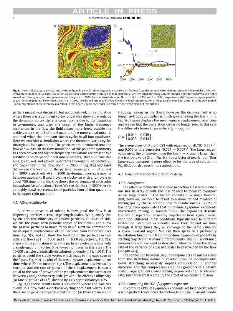
Fig. 8. 4-rollmillmixing: panels (a) and the inset figure in panel (b) show Lagrangian particle distributions from the numerical simulations (using 65,536 particles). Solutionsevolve from random initial data, simulation yields stable vortex rotating through all four quadrants. Particles originating in quadrants I (upper right) through IV (lower right)are colored blue, green, red, and yellow, respectively at t = 2000. Particle distribution for W i = 10 at t = 2150 and t = 3000, respectively. (b) The percentage of particlesof each color in quadrant I over time, 2000 < t < 3200. The dashed line at 1/4 shows the nearly equal representation of all quadrants over long times. τ1 is the slow period.(For interpretation of the references to colour in this figure legend, the reader is referred to the web version of this article.)

particle mixing was discussed, but not quantified, for a simulationwhere there was a dominant vortex, and it was shown that outsidethe dominant vortex there is some mixing due to the transitionto asymmetry, and after the onset of the higher-frequencyoscillations in the flow the fluid mixes more freely outside thestable vortex (i.e. in 3 of the 4 quadrants). A more global mixer isobtained when the dominant vortex cycles in all four quadrants.Here we consider a simulation where the dominant vortex cyclesthrough all four quadrants. The particles are introduced into theflow at t = 2000 in the flow simulation; at this point the symmetryhas been broken and higher-frequency oscillations are present.Wesubdivide the 2π-periodic cell into quadrants, label fluid particlesblue, green, red, and yellow (quadrants I through IV, respectively),and track them in the flow, for t > 2000. In Fig. 8(a) and inset(b) we see the location of the particle tracers at t = 2150 andt = 3000 respectively. At t = 2000 the dominant vortex is movingbetween quadrants II and I, cycling clockwise with a full cycle inabout 750 time units. Fig. 8(b) shows the percentage of each colorin quadrant I as a function of time.We see that for t & 3000 there isa roughly equal representation of particles from all four quadrantsin the upper right quadrant.

4.2. Effective diffusivity

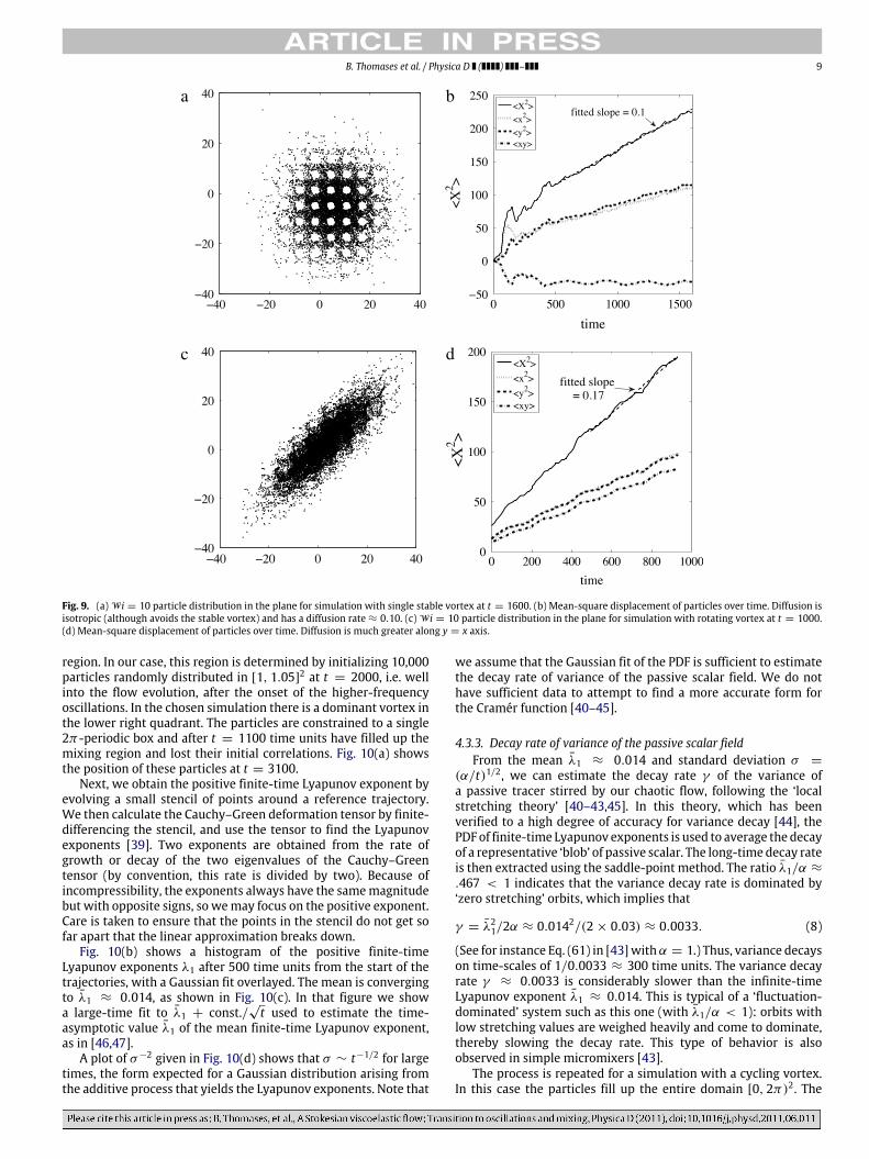
A relevant measure of mixing is how good the flow is atdispersing particles across large length scales. We quantify thisby the effective diffusivity of passive particles. To measure this,we tile the plane with periodic copies of the flow u and allowthe passive particles to move freely in R2. Next we compute themean-square displacement of the particles from the origin overtime. Fig. 9(a) and (c) show the location of the particles in twodifferent flows at t = 1600 and t = 1000 respectively. Fig. 9(a)arises from a simulation where the particles evolve in a flow witha single-quadrant vortex (the lower right one in this case). The10,000particles are initially distributed randomly in [1, 1.05]2. Theparticles avoid the stable vortex which leads to the gaps seen inthe figure. Fig. 9(b) is a plot of the mean-square displacement overtime, where ⟨X2

⟩ = mean(x2+y2). The displacement is eventuallyisotropic and the rate of growth of the x displacement is nearlyequal to the rate of growth of the y displacement; the correlationbetween x and y shows very little growth. The effective diffusivity(or rate of growth of ⟨X2

⟩, divided by 4) is approximately 0.025.Fig. 9(c) shows results from a simulation where the particles

evolve in a flow with a clockwise-cycling dominant vortex. Herethere are no gaps in the particle distribution (as there are no visible

trapping regions in the flow); however the displacement is nolonger isotropic, but rather is much greater along the line y = x.Fig. 9(d) again displays the mean-square displacement over timeand we see that the correlation ⟨xy⟩ is no longer zero. In this casethe diffusivity tensor D, given by 2Dij = ⟨xixj⟩, is

D =

0.044 0.0390.039 0.044

.

The eigenvalues of D are 0.083 with eigenvector (0.707 0.707)T ;and 0.005 with eigenvector (0.707 − 0.707)T . The larger eigen-value gives the diffusivity along the line y = x, and is larger thanthe isotropic value (from Fig. 9(a)) by a factor of nearly four. Thuslarge-scale transport is more effective for the type of solution inFig. 9(c), but also much more anisotropic.

4.3. Lyapunov exponents and variance decay

4.3.1. BackgroundThe effective diffusivity described in Section 4.2 is useful when

one has an array of rolls and it is desired to measure transportacross large scales. If the system consists of a single four-rollmill, however, we need to resort to a more refined measure ofmixing quality that is better suited to chaotic mixing [38,39]. Ithas long been appreciated that finite-time Lyapunov exponentscharacterize mixing in smooth flows. The exponents describethe rate of separation of nearby trajectories from a given initialcondition. Different initial conditions typically lead to differentfinite-time Lyapunov exponents, since they depend on time,though at large times they all converge to the same value fora given invariant region. We can then speak of a probabilitydistribution function (PDF) of finite-time Lyapunov exponents bystarting trajectories at many different points. This PDF is obtainednumerically and averaged as described below to obtain the decayrate of the variance of a passive scalar field advected by the flow(see [40–45]).

The connection between Lyapunov exponents andmixing arisesfrom the stretching nature of chaotic flows: in incompressibleflows stretching necessarily implies compression in anotherdirection, and this compression amplifies gradients of a passivescalar. Large gradients cause mixing to proceed at an acceleratedrate, since they greatly amplify the effect of molecular diffusion.

4.3.2. Computing the PDF of Lyapunov exponentsTo compute a PDFof Lyapunov exponents,we first need to select

a set of particle trajectories that belong to a single invariant chaotic

B. Thomases et al. / Physica D ( ) – 9

a b

c d

Fig. 9. (a) W i = 10 particle distribution in the plane for simulation with single stable vortex at t = 1600. (b) Mean-square displacement of particles over time. Diffusion isisotropic (although avoids the stable vortex) and has a diffusion rate ≈ 0.10. (c) W i = 10 particle distribution in the plane for simulation with rotating vortex at t = 1000.(d) Mean-square displacement of particles over time. Diffusion is much greater along y = x axis.

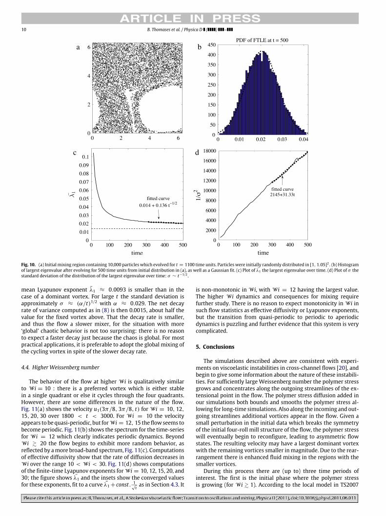
region. In our case, this region is determined by initializing 10,000particles randomly distributed in [1, 1.05]2 at t = 2000, i.e. wellinto the flow evolution, after the onset of the higher-frequencyoscillations. In the chosen simulation there is a dominant vortex inthe lower right quadrant. The particles are constrained to a single2π-periodic box and after t = 1100 time units have filled up themixing region and lost their initial correlations. Fig. 10(a) showsthe position of these particles at t = 3100.

Next, we obtain the positive finite-time Lyapunov exponent byevolving a small stencil of points around a reference trajectory.We then calculate the Cauchy–Green deformation tensor by finite-differencing the stencil, and use the tensor to find the Lyapunovexponents [39]. Two exponents are obtained from the rate ofgrowth or decay of the two eigenvalues of the Cauchy–Greentensor (by convention, this rate is divided by two). Because ofincompressibility, the exponents always have the samemagnitudebut with opposite signs, so wemay focus on the positive exponent.Care is taken to ensure that the points in the stencil do not get sofar apart that the linear approximation breaks down.

Fig. 10(b) shows a histogram of the positive finite-timeLyapunov exponents λ1 after 500 time units from the start of thetrajectories, with a Gaussian fit overlayed. The mean is convergingto λ1 ≈ 0.014, as shown in Fig. 10(c). In that figure we showa large-time fit to λ1 + const./

√t used to estimate the time-

asymptotic value λ1 of the mean finite-time Lyapunov exponent,as in [46,47].

A plot of σ−2 given in Fig. 10(d) shows that σ ∼ t−1/2 for largetimes, the form expected for a Gaussian distribution arising fromthe additive process that yields the Lyapunov exponents. Note that

we assume that the Gaussian fit of the PDF is sufficient to estimatethe decay rate of variance of the passive scalar field. We do nothave sufficient data to attempt to find a more accurate form forthe Cramér function [40–45].

4.3.3. Decay rate of variance of the passive scalar fieldFrom the mean λ1 ≈ 0.014 and standard deviation σ =

(α/t)1/2, we can estimate the decay rate γ of the variance ofa passive tracer stirred by our chaotic flow, following the ‘localstretching theory’ [40–43,45]. In this theory, which has beenverified to a high degree of accuracy for variance decay [44], thePDF of finite-time Lyapunov exponents is used to average the decayof a representative ‘blob’ of passive scalar. The long-time decay rateis then extracted using the saddle-point method. The ratio λ1/α ≈

.467 < 1 indicates that the variance decay rate is dominated by‘zero stretching’ orbits, which implies that

γ = λ21/2α ≈ 0.0142/(2 × 0.03) ≈ 0.0033. (8)

(See for instance Eq. (61) in [43]withα = 1.) Thus, variance decayson time-scales of 1/0.0033 ≈ 300 time units. The variance decayrate γ ≈ 0.0033 is considerably slower than the infinite-timeLyapunov exponent λ1 ≈ 0.014. This is typical of a ‘fluctuation-dominated’ system such as this one (with λ1/α < 1): orbits withlow stretching values are weighed heavily and come to dominate,thereby slowing the decay rate. This type of behavior is alsoobserved in simple micromixers [43].

The process is repeated for a simulation with a cycling vortex.In this case the particles fill up the entire domain [0, 2π)2. The

10 B. Thomases et al. / Physica D ( ) –

a b

c d

Fig. 10. (a) Initial mixing region containing 10,000 particles which evolved for t = 1100 time units. Particles were initially randomly distributed in [1, 1.05]2. (b) Histogramof largest eigenvalue after evolving for 500 time units from initial distribution in (a), as well as a Gaussian fit. (c) Plot of λ1 the largest eigenvalue over time. (d) Plot of σ thestandard deviation of the distribution of the largest eigenvalue over time: σ ∼ t−1/2 .

mean Lyapunov exponent λ1 ≈ 0.0093 is smaller than in thecase of a dominant vortex. For large t the standard deviation isapproximately σ ≈ (α/t)1/2 with α ≈ 0.029. The net decayrate of variance computed as in (8) is then 0.0015, about half thevalue for the fixed vortex above. That the decay rate is smaller,and thus the flow a slower mixer, for the situation with more‘global’ chaotic behavior is not too surprising: there is no reasonto expect a faster decay just because the chaos is global. For mostpractical applications, it is preferable to adopt the global mixing ofthe cycling vortex in spite of the slower decay rate.

4.4. Higher Weissenberg number

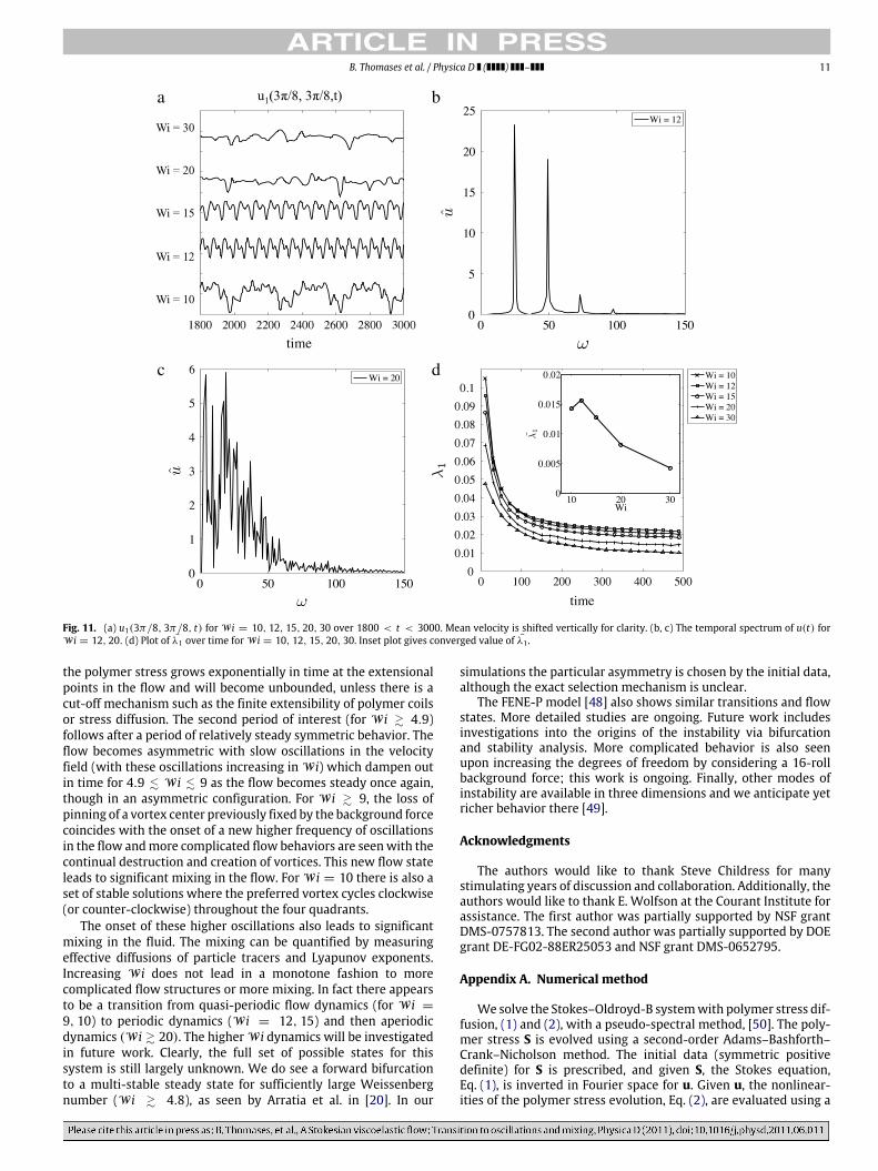
The behavior of the flow at higher W i is qualitatively similarto W i = 10 : there is a preferred vortex which is either stablein a single quadrant or else it cycles through the four quadrants.However, there are some differences in the nature of the flow.Fig. 11(a) shows the velocity u1(3π/8, 3π/8, t) for W i = 10, 12,15, 20, 30 over 1800 < t < 3000. For W i = 10 the velocityappears to be quasi-periodic, but forW i = 12, 15 the flow seems tobecome periodic. Fig. 11(b) shows the spectrum for the time-seriesfor W i = 12 which clearly indicates periodic dynamics. BeyondW i & 20 the flow begins to exhibit more random behavior, asreflected by amore broad-band spectrum, Fig. 11(c). Computationsof effective diffusivity show that the rate of diffusion decreases inW i over the range 10 < W i < 30. Fig. 11(d) shows computationsof the finite-time Lyapunov exponents forW i = 10, 12, 15, 20, and30; the figure shows λ1 and the insets show the converged valuesfor these exponents, fit to a curve λ1 + const. 1

√tas in Section 4.3. It

is non-monotonic in W i, with W i = 12 having the largest value.The higher W i dynamics and consequences for mixing requirefurther study. There is no reason to expect monotonicity in W i insuch flow statistics as effective diffusivity or Lyapunov exponents,but the transition from quasi-periodic to periodic to aperiodicdynamics is puzzling and further evidence that this system is verycomplicated.

5. Conclusions

The simulations described above are consistent with experi-ments on viscoelastic instabilities in cross-channel flows [20], andbegin to give some information about the nature of these instabili-ties. For sufficiently largeWeissenberg number the polymer stressgrows and concentrates along the outgoing streamlines of the ex-tensional point in the flow. The polymer stress diffusion added inour simulations both bounds and smooths the polymer stress al-lowing for long-time simulations. Also along the incoming and out-going streamlines additional vortices appear in the flow. Given asmall perturbation in the initial data which breaks the symmetryof the initial four-roll mill structure of the flow, the polymer stresswill eventually begin to reconfigure, leading to asymmetric flowstates. The resulting velocity may have a largest dominant vortexwith the remaining vortices smaller in magnitude. Due to the rear-rangement there is enhanced fluid mixing in the regions with thesmaller vortices.

During this process there are (up to) three time periods ofinterest. The first is the initial phase where the polymer stressis growing (for W i & 1). According to the local model in TS2007

B. Thomases et al. / Physica D ( ) – 11

a b

c d

Fig. 11. (a) u1(3π/8, 3π/8, t) for W i = 10, 12, 15, 20, 30 over 1800 < t < 3000. Mean velocity is shifted vertically for clarity. (b, c) The temporal spectrum of u(t) forW i = 12, 20. (d) Plot of λ1 over time for W i = 10, 12, 15, 20, 30. Inset plot gives converged value of λ1 .

the polymer stress grows exponentially in time at the extensionalpoints in the flow and will become unbounded, unless there is acut-off mechanism such as the finite extensibility of polymer coilsor stress diffusion. The second period of interest (for W i & 4.9)follows after a period of relatively steady symmetric behavior. Theflow becomes asymmetric with slow oscillations in the velocityfield (with these oscillations increasing in W i) which dampen outin time for 4.9 . W i . 9 as the flow becomes steady once again,though in an asymmetric configuration. For W i & 9, the loss ofpinning of a vortex center previously fixed by the background forcecoincides with the onset of a new higher frequency of oscillationsin the flow andmore complicated flow behaviors are seenwith thecontinual destruction and creation of vortices. This new flow stateleads to significant mixing in the flow. For W i = 10 there is also aset of stable solutions where the preferred vortex cycles clockwise(or counter-clockwise) throughout the four quadrants.

The onset of these higher oscillations also leads to significantmixing in the fluid. The mixing can be quantified by measuringeffective diffusions of particle tracers and Lyapunov exponents.Increasing W i does not lead in a monotone fashion to morecomplicated flow structures or more mixing. In fact there appearsto be a transition from quasi-periodic flow dynamics (for W i =

9, 10) to periodic dynamics (W i = 12, 15) and then aperiodicdynamics (W i & 20). The higher W i dynamics will be investigatedin future work. Clearly, the full set of possible states for thissystem is still largely unknown. We do see a forward bifurcationto a multi-stable steady state for sufficiently large Weissenbergnumber (W i & 4.8), as seen by Arratia et al. in [20]. In our

simulations the particular asymmetry is chosen by the initial data,although the exact selection mechanism is unclear.

The FENE-P model [48] also shows similar transitions and flowstates. More detailed studies are ongoing. Future work includesinvestigations into the origins of the instability via bifurcationand stability analysis. More complicated behavior is also seenupon increasing the degrees of freedom by considering a 16-rollbackground force; this work is ongoing. Finally, other modes ofinstability are available in three dimensions and we anticipate yetricher behavior there [49].

Acknowledgments

The authors would like to thank Steve Childress for manystimulating years of discussion and collaboration. Additionally, theauthors would like to thank E. Wolfson at the Courant Institute forassistance. The first author was partially supported by NSF grantDMS-0757813. The second author was partially supported by DOEgrant DE-FG02-88ER25053 and NSF grant DMS-0652795.

Appendix A. Numerical method

We solve the Stokes–Oldroyd-B systemwith polymer stress dif-fusion, (1) and (2), with a pseudo-spectral method, [50]. The poly-mer stress S is evolved using a second-order Adams–Bashforth–Crank–Nicholson method. The initial data (symmetric positivedefinite) for S is prescribed, and given S, the Stokes equation,Eq. (1), is inverted in Fourier space for u. Given u, the nonlinear-ities of the polymer stress evolution, Eq. (2), are evaluated using a

12 B. Thomases et al. / Physica D ( ) –

smooth filterwhich is applied in Fourier space before the quadraticterms aremultiplied in real space; see [51] for details. The polymerstress equation, Eq. (2), is considered in the form

∂tS = νpS + N(S,u),

where N(S,u) = −u · ∇S + (∇u S + S ∇uT ) −1

W i (S − I). Thepolymer stress is then discretized on the Fourier transform side

Sn+1− Sn

t= −νp|k|2

Sn+1+ Sn

2

+12[3N(Sn,un) − N(Sn−1,un−1)].

Note that νp ≡ 0 will yield the typical second-order Adams–Bashforth scheme.We find that positive definiteness ismaintainedin all of our simulations and the time-steppingwas verified to havesecond-order accuracy. For W i ≤ 10, with νp = 10−3 a spatialdiscretization of n2

= 2562 is sufficient to resolve the spatialaccuracy to O(10−12), for the long times necessary for this study.For W i > 10 we scale νp =

.01W i , and there is some loss of accuracy,

however for W i ≤ 30, the spatial accuracy is still resolved toO(10−4) with the diffusion scaled as above.

An additional component to our numerical study is the needto track particles in the flow. We use second-order spatialinterpolation to obtain the velocity field between grid cells, andupdate the particles with this velocity using a second-ordermethod.

Appendix B. Choice and calibration of model

In this studyweuse the Stokes–Oldroyd-B systemwith polymerstress diffusion given by Eqs. (1) and (2). This model differsfrom the standard Stokes–Oldroyd-B model by the addition ofthe polymer stress diffusion term νpS. In the derivation of theOldroyd-B model from kinetic theory [26] it is assumed that thespatial diffusion of the probability density function is quite smallcompared with the diffusion in phase space, and hence this termis usually ignored. It is included here in an approximate form.In [36] it was shown that a similar modification of the polymerstress equation can be justified from microscopic principles (atleast for steady solutions) and will yield smooth solutions for thepolymer stress as long as the polymer stress remains bounded. Inour simulations we see that the addition of this term keeps thepolymer stress bounded and smooth dynamically as well, whereasfor νp = 0 the polymer stress will grow at least exponentially atextensional points in the flow for sufficiently large Weissenbergnumber. We choose the size νp to so that the solutions to theStokes–Oldroyd-B model with polymer diffusion compare wellwith solutions which maintain finite extensibility. These solutionscome from the FENE-P model described below.

FENE (Finitely Extensible Nonlinear Elastic) models are amodelof viscoelastic fluids which incorporate finite extension of polymercoils in their derivation. In the FENE model [27] the response of apolymer coil is no longer a linear Hookean spring, as for Oldroyd-B,but is given by Warner’s force law [52]

F =κR

1 − (R2/ℓ2),

where κ is the spring constant, R is the end to end vectorrepresenting the polymer coil, and ℓ is the maximum allowedextension length. This force law penalizes distension of thepolymer coils (given by the end to end vector R). However, unlikeOldroyd-B, this model does not close under the macroscopicassumptions and therefore computations of the full FENE modelrequire a coupling of the microscopic scale, to simulate thepolymers, with themacroscopic flow field. These computations are

prohibitively expensive in general. A simple way to obtain a closedmacroscopic model is via pre-averaging, i.e. choosing a force lawof the form

F =κR

1 − (⟨R⟩2 /ℓ2)

,

where the brackets indicate taking the average over the probabilitydensity function of R. This yields the closed macroscopic FENE-Pmodel [48] which does give a finite extension length. This artificialcut-off of tr S, however does not smooth the polymer stresssufficiently to make long-time computations reasonable, [28].

Simulations of FENE-P were done in TS2007 in a 2D periodicextensional flow with the four-roll mill geometry, to compare di-rectly with the similar results for the standard Stokes–Oldroyd-B model. In these simulations tr S remained bounded for allWeissenberg number. However singularities still arise exponen-tially in time in the polymer stress gradient for sufficiently largeWeissenberg number. These singularities appeared as either cusps(1/2 . W i . 1) or corners (W i & 1). Although the FENE-P modeldoes maintain a finite polymer stress at all time, the singularitiesin the polymer stress gradients cause the same numerical difficul-ties as the Stokes–Oldroyd-B model for long-time simulations ofthe dynamic equations, which suggests a potentially non-physicalcut-off mechanism.

We note that the use of νp > 0 does not modify the polymerstress significantly outside a small region of the extensional pointsin the flow. In TS2007 it was observed that in the Oldroyd-Bmodelfor sufficiently large W i the polymer stress is diverging, but it wasalso noted that tr S gets large on a set of exponentially shrinkingmeasure. Outside of this set tr S does reach a steady state. Thewidth of the divergent region decreases exponentially in time andthe net force from this region also decreases in time. This mayexplain why the unsteady region (with νp = 0) has a decreasingeffect on the flow. Given this observation it seemsmore importantthat the polymer stress in the modified system (νp > 0) behavesqualitatively like the polymer stress from the Stokes–Oldroyd-Bsystem outside a small region near the stagnation point, than thatthe exact details of the polymer stress match very close to thestagnation point.

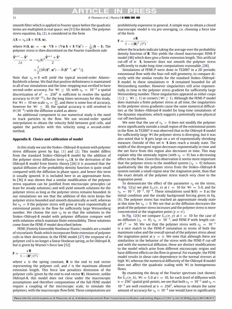
To demonstrate the effect of the parameter νp on the stress,in Fig. 12(a) we plot S11(π, x) at t = 10 for W i = 5.0, and forνp = 10−2, 10−3, 10−4. These simulations used S(0) = I as theinitial condition and the steady background forcing given in Eq.(6). The polymer stress has reached an approximate steady stateat this time for νp > 0. We see that as the diffusion decreases thepeak of the polymer stress increases and the polymer stress ismoreconcentrated at the stagnation point (y = π ).

In Fig. 12(b) we compare S11(π, y) at t = 10 for the case ofno diffusion (νp = 0), νp = 10−3, and FENE-P with length cut-off ℓ2

= 50. We see that the polymer stress with νp = 10−3

is a nice match to the FENE-P simulation in terms of both themaximum value and the overall spread of the polymer stress aboutthe stagnation point at y = π . We note that although there aresimilarities in the behavior of the stress with the FENE-P cut-offand with the numerical diffusion, these are distinct modificationsto the model which arise from different microscopic origins andhave different effects on the flow in general. For example; the FENEmodel results in shear-rate-dependence in the normal stresses athighW i, whereas the numerical diffusivity of the Oldroyd-Bmodeldoes not affect the quadratic scaling with W i in homogeneousflows.

By examining the decay of the Fourier spectrum (not shown)for S11(π, k), W i = 5.0 at t = 10, for each level of diffusion withn = 2562 spatial grid-points, we see that both νp = 10−2 and νp =

10−3 are well resolved at n = 2562, whereas to obtain the sameamount of accuracy for νp = 10−4 one would have to significantly

B. Thomases et al. / Physica D ( ) – 13

a b

Fig. 12. (a) Plot of S11(π, y) at steady state for W i = 5.0 comparing different amounts of diffusion, ranging from νp = 10−2, 10−3, 10−4 . (b) Plot of S11(π, y) at t = 10 forW i = 5.0 comparing no diffusion (νp = 0), FENE-P (with length cut-off ℓ2

= 50), and diffusion νp = 10−3..

increase n, and hence computation time. The long-time simula-tionswe are after can be accomplished reasonably using n2

= 2562

and hence the choice of νp = 10−3 is sufficient both for numericalconsiderations and for the favorable comparison with FENE-P.

References

[1] A. Groisman, V. Steinberg, Elastic turbulence in a polymer solution flow,Nature 405 (2000) 53–55.

[2] A. Groisman, V. Steinberg, Efficient mixing at low Reynolds numbers usingpolymer additives, Nature 410 (2001) 905–908.

[3] A. Groisman, V. Steinberg, Elastic turbulence in curvilinear flows of polymersolutions, New. J. Phys. 4 (2004) 74437.

[4] E.M. Purcell, Life at low Reynolds number, Amer. J. Phys. 45 (1977) 3–11.[5] A. Groisman, S. Quake, A microfluidic rectifier: anisotropic flow resistance at

low Reynolds numbers, Phys. Rev. Lett. 92 (2004) 094501.[6] J. Teran, L. Fauci, M. Shelley, Peristaltic pumping and irreversibility of a

Stokesian viscoelastic fluid, Phys. Fluids 20 (2008) 073101.[7] E. Shaqfeh, S.J.Muller, R.G. Larson, A purely elastic transition in Taylor–Couette

flow, Rheol. Acta 28 (1989) 499.[8] G.H. McKinley, J.A. Byars, R.A. Brown, R.C. Armstrong, Observations on the

elastic instability in cone-and-plate and parallel-plate flows of a polyisobuty-lene Boger fluid, J. Non-Newton. Fluid Mech. 40 (1991) 201.

[9] A. Oztekin, R.A. Brown, Instability of a viscoelastic fluid between rotatingparallel disks: analysis for the Oldroyd-B fluid, J. Fluid Mech. 255 (1993) 473.

[10] J.A. Byars, A. Öztekin, R.A. Brown, G.H. McKinley, Spiral instabilities in theflow of highly elastic fluids between rotating parallel disks, J. Fluid Mech. 271(1994) 173.

[11] Peyman Pakdel, GarethH.McKinley, Elastic instability and curved streamlines,Phys. Rev. Lett. 77 (12) (1996) 2459–2462.

[12] E. Shaqfeh, Purely elastic instabilities in viscometric flows, Annu. Rev. FluidMech. 28 (1996) 129.

[13] G.H. McKinley, T. Sridhar, Filament-stretching rheometry of complex fluids,Annu. Rev. Fluid Mech. 34 (2002) 375.

[14] R.G. Owens, T.N. Phillips, Computational Rheology, Imperial College Press,2002.

[15] N. Phan-Thien, Coaxial-disk flow of and Oldroyd-B fluid: Exact solution andstability, J. Non-Newton. Fluid Mech. 13 (1983) 325.

[16] J.J. Magda, R.G. Larson, A transition occurring in ideal elastic liquids duringshear flow, J. Non-Newton. Fluid Mech. 30 (1988) 1.

[17] D.E. Smith, H.P. Babcock, S. Chu, Single-polymer dynamics in steady shearflow, Science 283 (1999) 1724.

[18] J.P. Rothstein, G.H. McKinley, The axisymmetric contraction expansion: therole of extensional rheology on vortex growth dynamics and the enhancedpressure drop, J. Non-Newton. Fluid Mech. 98 (2001) 33.

[19] C. Schroeder, H. Babcock, E. Shaqfeh, S. Chu, Observation of polymer confor-mation hysteresis in extensional flow, Science 301 (2003) 1515.

[20] P.E. Arratia, C.C. Thomas, J. Diorio, J.P. Gollub, Elastic instabilities of polymersolutions in cross-channel flow, Phys. Rev. Letters 96 (2006) 144502.

[21] A. Groisman, M. Enzelberger, S. Quake, Microfluidic memory and controldevices, Science 300 (2003) 955.

[22] L.E. Rodd, T.P. Scott, D.V. Boger, J.J. Cooper-White, G.H. McKinley, The inertio-elastic planar entry flow of low-viscosity elastic fluids in micro-fabricatedgeometries, J. Non-Newton. Fluid Mech. 129 (2005) 1.

[23] B. Thomases, M. Shelley, Transition to mixing and oscillations in a Stokesianviscoelastic flow, Phys. Rev. Lett. 103 (2009) 094501.

[24] L. Xi, M. Graham, A mechanism for oscillatory instability in viscoelasticcross-slot flow, J. Fluid Mech. 622 (2009) 145–165.

[25] S. Berti, A. Bistagnino, G. Boffetta, A. Celani, S. Musacchio, Two-dimensionalelastic turbulence, Phys. Rev. E 77 (2008) 055306.

[26] M. Doi, S. Edwards, The Theory of Polymer Dynamics, Oxford University Press,New York, 1986.

[27] R.G. Larson, The Structure and Rheology of Complex Fluids, Oxford UniversityPress, 1998.

[28] B. Thomases, M. Shelley, Emergence of singular structures in Oldroyd-B fluids,Phys. Fluids 19 (2007) 103103.

[29] E.J. Hinch, Mechanical models of dilute polymer solutions in strong flows,Phys. Fluids 20 (1977) S22–S30.

[30] M. Chertkov, Polymer stretching by turbulence, Phys. Rev. Lett. 84 (20) (2000)4761–4764.

[31] Jean-Luc Thiffeault, Finite extension of polymers in turbulent flow, Phys. Lett.A 308 (5–6) (2003) 445–450.

[32] M. Renardy, A comment on smoothness of viscoelastic stresses, J. Non-NewtFluid Mech. 138 (2006) 204–205.

[33] C.-Y. Lu, P.D. Olmsted, R.C. Ball, Effects of nonlocal stress on the determinationof shear banding flow, Phys. Rev. Lett. 84 (2000) 642.

[34] E.J. Hinch, Uncoiling a polymer molecule in a strong extensional flow,J. Non-Newton. Fluid Mech. 54 (1994) 209.

[35] J.M. Rallison, Dissipative stresses in dilute polymer solutions, J. Non-Newton.Fluid Mech. 68 (1996) 61.

[36] A.W. El-Kareh, L.G. Leal, Existence of solutions for all Deborah numbers fora non-Newtonian model modified to include diffusion, J. Non-Newton. FluidMech. 33 (1989) 257.

[37] J.M. Rallison, E.J. Hinch, Do we understand the physics in the constitutiveequation? J. Non-Newt Fluid Mech. 29 (1988) 37–55.

[38] H. Aref, Stirring by chaotic advection, J. Fluid Mech. 143 (1984) 1–21.[39] J.M. Ottino, The Kinematics of Mixing: Stretching, Chaos, and Transport,

Cambridge University Press, Cambridge, UK, 1989.[40] T.M. Antonsen Jr., Z. Fan, E. Ott, E. Garcia-Lopez, The role of chaotic orbits in

the determination of power spectra, Phys. Fluids 8 (11) (1996) 3094–3104.[41] E. Balkovsky, A. Fouxon, Universal long-time properties of Lagrangian statis-

tics in the Batchelor regime and their application to the passive scalarproblem, Phys. Rev. E 60 (4) (1999) 4164–4174.

[42] J. Sukhatme, R.T. Pierrehumbert, Decay of passive scalars under the actionof single scale smooth velocity fields in bounded two-dimensional do-mains: from non-self-similar probability distribution functions to self-similareigenmodes, Phys. Rev. E 66 (November) (2002) 056032.

[43] Jean-Luc Thiffeault, Scalar decay in chaotic mixing, in: J.B. Weiss, A. Proven-zale (Eds.), Transport and Mixing in Geophysical Flows, in: Lecture Notes inPhysics, vol. 744, Springer, Berlin, 2008, pp. 3–35.

[44] Y.-K. Tsang, T.M. Antonsen Jr., E. Ott, Exponential decay of chaotically advectedpassive scalars in the zero diffusivity limit, Phys. Rev. E 71 (2005) 066301.

[45] P.H. Haynes, J. Vanneste, What controls the decay of passive scalars in smoothflows? Phys. Fluids 17 (2005) 097103.

[46] Xian Zhu Tang, Allen H. Boozer, Finite time Lyapunov exponent and advec-tion–diffusion equation, Physica D 95 (1996) 283–305.

[47] Jean-Luc Thiffeault, P.J. Morrison, The twisted top, Phys. Lett. A 283 (5–6)(2001) 335–341.

[48] R.B. Bird, P.J. Dotson, N.L. Johnson, Polymer solution rheology based on afinitely extensible bead-spring chain model, J. Non-Newt Fluid Mech. 7 (1980)213–235.

[49] R.G. Larson, S.J. Muller, E.S.G. Shaqfeh, A purely elastic instability in Tay-lor–Couette flow, J. Fluid Mech. 218 (1990) 573–600.

[50] Roger Peyret, Spectral Methods for Incompressible Viscous Flow, Springer,New York, 2002.

[51] T.Y. Hou, R. Li, Computing nearly singular solutions using pseudo-spectralmethods, J. Comput. Phys. 226 (2007) 379–397.

[52] H.R. Warner, Kinetic theory and rheology of dilute suspensions of finitelyextensible dumbbells, Ind. Eng. Chem. Fundam. 11 (1972) 379–387.