A sparse-response deep belief network based on rate distortion theory

Nan-Nan Ji, Jiang-She Zhang n, Chun-Xia ZhangSchool of Mathematics and Statistics, Xi'an Jiaotong University, Xi'an Shaanxi 710049, China

a r t i c l e i n f o

Article history:Received 26 April 2013Accepted 26 March 2014Available online 12 April 2014

Keywords:Deep belief networkKullback–Leibler divergenceInformation entropyRate distortion theoryUnsupervised feature learning

a b s t r a c t

Deep belief networks (DBNs) are currently the dominant technique for modeling the architectural depthof brain, and can be trained efficiently in a greedy layer-wise unsupervised learning manner. However,DBNs without a narrow hidden bottleneck typically produce redundant, continuous-valued codes andunstructured weight patterns. Taking inspiration from rate distortion (RD) theory, which encodesoriginal data using as few bits as possible, we introduce in this paper a variant of DBN, referred to assparse-response DBN (SR-DBN). In this approach, Kullback–Leibler divergence between the distributionof data and the equilibrium distribution defined by the building block of DBN is considered as adistortion function, and the sparse response regularization induced by L1-norm of codes is used toachieve a small code rate. Several experiments by extracting features from different scale image datasetsshow that our approach SR-DBN learns codes with small rate, extracts features at multiple levels ofabstraction mimicking computations in the cortical hierarchy, and obtains more discriminative represen-tation than PCA and several basic algorithms of DBNs.

& 2014 Elsevier Ltd. All rights reserved.

1. Introduction

Recent neuroscience findings [1–6] have provided insight intothe principles governing information representation in the mam-mal brain, leading to new ideas for designing systems to effectivelyrepresent information. One of the key findings is that the mammalbrain is organized in a deep architecture. Given an input percept,it is represented with multiple levels of abstraction, each levelcorresponding to a different area of cortex. By using these abstractfeatures learned through the deep architecture, human achievesperfect performance on many real-world tasks such as objectrecognition, detection, prediction, and visualization. In currentmachine learning community, how to imitate this hierarchicalarchitecture of mammal brain to obtain good representation ofdata in order to improve the performance of a learning algorithmhas become an essential issue.

Recently, deep learning has become the dominant technique tolearn good information representation that exhibits similar char-acteristics to that of the mammal brain. It has gained significantinterest for building hierarchical representations from unlabeleddata. A deep architecture consists of feature detector units arrangedin multiple layers: lower layers detect simple features and feed intohigher layers, which in turn detect more complex features. Inparticular, deep belief network (DBN), the most popular approach

of deep learning, is a multilayer generative model in which eachlayer encodes statistical dependencies among the units in the layerbelow, and it can be trained to maximize (approximately) thelikelihood of its training data. So far, there have been a great dealof DBN models being proposed. For example, Hinton et al. [7]proposed an algorithm based on learning individual layers of ahierarchical probabilistic graphical model from the bottom up.Bengio et al. [8] proposed a similar greedy algorithm on the basisof auto-encoders. Ranzato et al. [9] developed an energy-basedhierarchical algorithm, using a sequence of sparsified auto-enco-ders/decoders. Particularly, the model proposed by Hinton et al. is abreakthrough for training deep networks. It can be viewed as acomposition of simple learning modules, each of which is arestricted Boltzmann machine (RBM) that contains a layer of visibleunits representing observable data and a layer of hidden unitslearned to represent features that capture higher-order correlationsin the data [10]. Nowadays, DBNs have been successfully applied toa variety of real-world applications, including hand-written char-acter recognition [7,11], text representation [12], audio eventclassification, object recognition [13], human motion capture data[14,15], information retrieval [16], machine transliteration [17],speech recognition [18–20] and various visual data analysis tasks[21–23].

Although DBNs have demonstrated promising results in learn-ing good codes or representations, DBNs without constraints on thehidden layers may produce redundant, continuous-valued codesand unstructured weight patterns. Some scholars attempted tofurther improve DBNs' performance according to add constraints

Contents lists available at ScienceDirect

journal homepage: www.elsevier.com/locate/pr

Pattern Recognition

http://dx.doi.org/10.1016/j.patcog.2014.03.0250031-3203/& 2014 Elsevier Ltd. All rights reserved.

n Corresponding author.E-mail address: jszhang@mail.xjtu.edu.cn (J.-S. Zhang).

Pattern Recognition 47 (2014) 3179–3191

on the representations [24–30]. Among them, introducing thenotion of sparsity makes DBN present state-of-the-art resultsbecause sparse representation is able to obtain succinct codesand structured weight patterns. Given images, sparse DBN is ableto discover low-level structures such as edges, as well as high-levelstructures such as corners, local curvatures, and shapes.

Sparsity was first proposed as a model of simple cells in thevisual cortex [31]. Up to now, it has been a key element of DBNslearning through exploiting a variant of auto-encoders, RBM, orother unsupervised learning algorithms. In practice, there aremany ways to enforce some form of sparsity on the hidden layerrepresentation of a deep architecture. The first successful deeparchitecture exploiting sparsity of representation involved auto-encoders [9]. Sparsity was achieved with a so-called sparsifyinglogistic, by which the codes are obtained with a nearly saturatinglogistic whose offset is adapted to maintain a low average numberof times that the code is significantly non-zero. One year later thesame group introduced a somewhat simple variant [28] throughassigning a Student-t prior on the coders. In the past, the Student-tprior was used to obtain sparse MAP estimates for the codesgenerating an input [29] in computational neuroscience models ofthe V1 visual cortex area. Another approach also related tocomputational neuroscience involves two levels of sparse RBMs[24]. Sparsity is achieved with a regularization term that penalizesa deviation of the expected activation of hidden units from a fixedlow-level. One level of sparse coding of images results in filtersvery similar to those seen in V1. When training a sparse deepbelief network, the second level appears to detect visual featuressimilar to those observed in area V2 of visual cortex.

From the point of view of information theory, one of the majorprinciples for finding concise representations is rate distortion (RD)theory [32], which focuses on the problem of determining minimalamount of information that should be communicated over a channel,so that a compressed representation of the original data can beapproximately reconstructed at the output data without exceeding agiven distortion. Sparse coding methods can be interpreted as specialcases of RD theory [33]. For deep multi-layer neural networks,hidden layers without narrow bottleneck may result in redundantand continuous-valued codes [34]. We hold that incorporating theconstraint of a minimum rate of information flow into the trainingprocess of multi-layer neural networks is able to make networksobtain succinct representations. From this point of view, we proposein this paper a novel version of sparse DBNs for unsupervised featureextraction by taking inspiration from the idea of RD theory. In DBNs,activation probability of the hidden units over a data vector is alwaysregarded as its representation or code. Therefore, in our approach,a small code rate is achieved by adding a constraint on the activationprobability of hidden units. The used constraint is L1-norm of thisactivation probability. Meanwhile, Kullback–Leibler divergencebetween the distribution of data and the equilibrium distributiondefined by the building block of DBN is considered as a measurementof distortion. More specifically, the novel approach is implementedby a trade-off between the L1 regularizer and the Kullback–Leiblerdivergence. The novel approach has the advantages that representa-tions with small information rate can be automatically learnt and thehierarchical representations (which mimics computations in thecortical hierarchy) can be obtained. Furthermore, compared to PCAand several basic algorithms of DBN, the new approach learns morediscriminative representations.

The remainder of this paper is organized as follows. We firstdescribe the DBN's structure and building block, RBM, with theirlearning rules in Section 2. Section 3 introduces the novel sparseDBN based on RD theory, and provides its learning rule. In Section 5,the novel sparse DBN is compared with several methods qualita-tively (the hierarchical bases learned by algorithms) and quantita-tively (the classification performance of subsequently built

classifier, starting from the representations obtained by unsuper-vised learning). Finally, this paper is concluded with a summaryand some directions for further research in Section 6.

2. Deep belief network (DBN) and its building block

DBNs are probabilistic generative models that contain manylayers of hidden variables, in which each layer captures high-order-correlations between the activities of hidden features in thelayer below. A key feature of this algorithm is its greedy layer-by-layer training that can be repeated several times to learn a deep,hierarchical model. The main building block of a DBN is a bipartiteundirected graphical model called the Restricted BoltzmannMachine (RBM). In this section, we provide a brief technicaloverview of RBM and the greedy learning algorithm for DBNs.

2.1. Restricted Boltzmann machine (RBM)

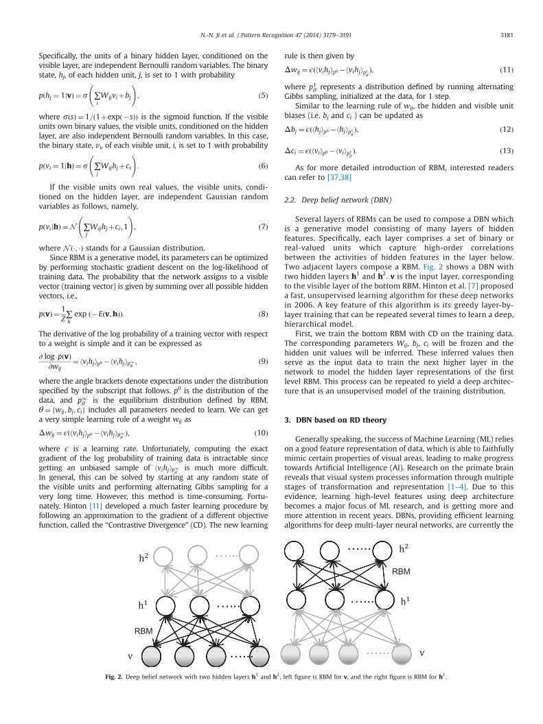
RBM [10,11,35,36] is a two-layer, bipartite, undirected graphicalmodel with a set of (binary or real-valued) visible units (randomvariables) v of dimension D representing observable data, and a setof binary hidden units (random variables) h of dimension Klearned to represent features that capture higher-order correla-tions in the observable data. These two layers are connected by asymmetrical weight matrix WARD�K , whereas there are no con-nections within a layer. Fig. 1 illustrates the undirected graphicalmodel of an RBM.

RBM can be viewed as a Markov random field that tries torepresent input data with hidden units. Here, the weights encode astatistical relationship between the hidden units and the visibleunits. The joint distribution over the visible and hidden units isdefined by

Pðv;hÞ ¼ 1Zexp ð�Eðv;hÞÞ; ð1Þ

Z ¼∑v∑hexp ð�Eðv;hÞÞ; ð2Þ

where Z is a normalization constant. Eðv;hÞ denotes the energy ofthe state ðv;hÞ. If the visible units are binary-valued, the energyfunction can be defined as

Eðv;hÞ ¼ � ∑D

i ¼ 1∑K

j ¼ 1viWijhj� ∑

K

j ¼ 1bjhj� ∑

D

i ¼ 1civi; ð3Þ

where bj and ci are respectively hidden and visible unit biases.If the visible units are real-valued, we can define the energyfunction by adding a quadratic term to make the distribution welldefined, that is,

Eðv;hÞ ¼ 12

∑D

i ¼ 1v2i � ∑

D

i ¼ 1∑K

j ¼ 1viWijhj� ∑

K

j ¼ 1bjhj� ∑

D

i ¼ 1civi: ð4Þ

From the energy function, we can see that the hidden units hj areindependent of each other when conditioning on v since there are nodirect connections between hidden units. Similarly, the visible unitsvi are also independent of each other when conditioning on h.

Fig. 1. Undirected graphical model of an RBM.

N.-N. Ji et al. / Pattern Recognition 47 (2014) 3179–31913180

Specifically, the units of a binary hidden layer, conditioned on thevisible layer, are independent Bernoulli random variables. The binarystate, hj, of each hidden unit, j, is set to 1 with probability

pðhj ¼ 1jvÞ ¼ s ∑iWijviþbj

!; ð5Þ

where sðsÞ ¼ 1=ð1þexpð�sÞÞ is the sigmoid function. If the visibleunits own binary values, the visible units, conditioned on the hiddenlayer, are also independent Bernoulli random variables. In this case,the binary state, vi, of each visible unit, i, is set to 1 with probability

pðvi ¼ 1jhÞ ¼s ∑jWijhjþci

!: ð6Þ

If the visible units own real values, the visible units, condi-tioned on the hidden layer, are independent Gaussian randomvariables as follows, namely,

pðvijhÞ ¼N ∑jWijhjþci;1

!; ð7Þ

where N ð�; �Þ stands for a Gaussian distribution.Since RBM is a generative model, its parameters can be optimized

by performing stochastic gradient descent on the log-likelihood oftraining data. The probability that the network assigns to a visiblevector (training vector) is given by summing over all possible hiddenvectors, i.e.,

pðvÞ ¼ 1Z∑hexp ð�Eðv;hÞÞ: ð8Þ

The derivative of the log probability of a training vector with respectto a weight is simple and it can be expressed as

∂ log pðvÞ∂wij

¼ ⟨vihj⟩p0 � ⟨vihj⟩p1θ ; ð9Þ

where the angle brackets denote expectations under the distributionspecified by the subscript that follows. p0 is the distribution of thedata, and p1θ is the equilibrium distribution defined by RBM.θ¼ fwij; bj; cig includes all parameters needed to learn. We can geta very simple learning rule of a weight wij as

Δwij ¼ ϵð⟨vihj⟩p0 � ⟨vihj⟩p1θ Þ; ð10Þ

where ϵ is a learning rate. Unfortunately, computing the exactgradient of the log probability of training data is intractable sincegetting an unbiased sample of ⟨vihj⟩p1θ is much more difficult.In general, this can be solved by starting at any random state ofthe visible units and performing alternating Gibbs sampling for avery long time. However, this method is time-consuming. Fortu-nately, Hinton [11] developed a much faster learning procedure byfollowing an approximation to the gradient of a different objectivefunction, called the “Contrastive Divergence” (CD). The new learning

rule is then given by

Δwij ¼ ϵð⟨vihj⟩p0 � ⟨vihj⟩p1θÞ; ð11Þ

where p1θ represents a distribution defined by running alternatingGibbs sampling, initialized at the data, for 1 step.

Similar to the learning rule of wij, the hidden and visible unitbiases (i.e. bj and ci ) can be updated as

Δbj ¼ ϵð⟨hj⟩p0 �⟨hj⟩p1θÞ; ð12Þ

Δci ¼ ϵð⟨vi⟩p0 � ⟨vi⟩p1θÞ: ð13Þ

As for more detailed introduction of RBM, interested readerscan refer to [37,38]

2.2. Deep belief network (DBN)

Several layers of RBMs can be used to compose a DBN whichis a generative model consisting of many layers of hiddenfeatures. Specifically, each layer comprises a set of binary orreal-valued units which capture high-order correlationsbetween the activities of hidden features in the layer below.Two adjacent layers compose a RBM. Fig. 2 shows a DBN withtwo hidden layers h1 and h2. v is the input layer, correspondingto the visible layer of the bottom RBM. Hinton et al. [7] proposeda fast, unsupervised learning algorithm for these deep networksin 2006. A key feature of this algorithm is its greedy layer-by-layer training that can be repeated several times to learn a deep,hierarchical model.

First, we train the bottom RBM with CD on the training data.The corresponding parameters Wij, bj, ci will be frozen and thehidden unit values will be inferred. These inferred values thenserve as the input data to train the next higher layer in thenetwork to model the hidden layer representations of the firstlevel RBM. This process can be repeated to yield a deep architec-ture that is an unsupervised model of the training distribution.

3. DBN based on RD theory

Generally speaking, the success of Machine Learning (ML) relieson a good feature representation of data, which is able to faithfullymimic certain properties of visual areas, leading to make progresstowards Artificial Intelligence (AI). Research on the primate brainreveals that visual system processes information through multiplestages of transformation and representation [1–4]. Due to thisevidence, learning high-level features using deep architecturebecomes a major focus of ML research, and is getting more andmore attention in recent years. DBNs, providing efficient learningalgorithms for deep multi-layer neural networks, are currently the

Fig. 2. Deep belief network with two hidden layers h1 and h2, left figure is RBM for v, and the right figure is RBM for h1.

N.-N. Ji et al. / Pattern Recognition 47 (2014) 3179–3191 3181

dominant technique for learning high-level features efficiently andeffectively.

However, DBNs without constraints on the hidden layers mayproduce redundant, continuous-valued codes and unstructuredweight patterns. From this point of view, a lot of theories andmethods in ML research have been developed for finding succinctcodes and structured weight patterns [9,24,28,39–44]. One of themajor principles in information theory for finding succinct codes israte distortion (RD) theory [32] which explores effective coding ofthe original data, that is, an encoding scheme using as few bits aspossible while maintaining the similarity between the originaldata and the decoded data within a certain allowable distortionlevel.

In this section, based on the idea of RD theory, we try toincorporate the learning of representation with a small code rateinto the training of DBNs by adding constraints on each hiddenlayer. Because DBN can be trained efficiently by a greedy layer-wise unsupervised learning procedure, i.e. one hidden layer istrained at a time by a RBM, incorporating constraints into thehidden layers of DBN can be carried out by adding constraint onthe hidden layer of each stacked RBM.

3.1. Rate distortion theory

RD theory is an information theoretic framework that findsconcise representations for input data such that the similaritybetween the original data and the decoded data falls into a certainallowable distortion level.

Let vARn be an input data and zARm be its representation orcode. Upper cases V and Z are used to represent the correspondingrandom variables. Given a distortion function d : Rn � Rm-R and adistortion upper limit D, the RD theory is formally stated as anoptimization problem with respect to the conditional probabilitypðZjVÞ:minpðZjVÞ

IðV;ZÞ

s:t: E½dðV;ZÞ�rD; ð14Þwhere IðV;ZÞ denotes the mutual information between V and Z,representing the rate of compression, i.e., code rate, and theexpectation E½dðV;ZÞ� is taken with respect to the joint distributionpðV;ZÞ. The dual formulation of this problem is

min E½dðV;ZÞ�s:t: IðV;ZÞrT ; ð15Þ

which is to find a coding scheme within a given rate such that theexpected distortion between the original data and the datadecoded from z is minimized.

3.2. Sparse-response RBM based on RD theory

Note that the mutual information IðV;ZÞ measures the informa-tion shared by the variables V and Z, and it can be calculated asIðV;ZÞ ¼HðZÞ�HðZjVÞ. Here, HðZÞ stands for the informationentropy of the random variable Z, and HðZjVÞ denotes the condi-tional entropy. Furthermore, if we consider a deterministic codingscheme v-z, then IðV;ZÞ ¼HðZÞ�HðZjVÞ ¼HðZÞ holds. As forRBMs, activation probability of the hidden units for a trainingvector is always regarded as its representation or code. Therefore,the code scheme obtained by RBM is deterministic. So, in ourapproach, we have IðV;ZÞ ¼HðZÞ, that is to say, minimum mutualinformation IðV;ZÞ in the RD theory can be transformed into theminimization of entropy HðZÞ.

In information theory, the entropy of the random variable Z,HðZÞ, is a measure of the uncertainty in Z. If some constraints areimposed on Z, then the uncertainty of this variable is reduced, and

the information entropy decreases. Based on the above analysis,we will reduce the information entropy of the random variable Zby a constraint, E½‖Z‖11�rη, that is, sparse representation is used toachieve a small code rate. Concretely, L1 regularization term on theactivation probability of hidden units (i.e. ‖Pðh¼ 1jvÞ‖1) isexploited to reduce the information entropy of representationslearn by RBM. In this way, the sparseness of representation,E½‖Z‖11�rη, corresponds to the small rate IðV;ZÞrT .

Distortion dðv; zÞ in the RD theory is considered as an errormeasure for representing the data v by the data decoded from z. Inmost cases, this distortion measure is defined as dðv; zÞ≔‖v�Bz‖2,where B is usually searched so that the reconstruction error isminimized. In our approach, because RBM is a probabilistic modeland can be viewed as a Markov random field, we will use theKullback–Leibler divergence, KLðp0 Jp1θ Þ, between the distributionof the data, p0, and the equilibrium distribution defined by a RBM,p1θ , to measure the error for representing the original data v by thedecoded data from the activation probability of hidden unitsPðh¼ 1jvÞ.

As described above, we consider the Kullback–Leibler diver-gence between the original data's distribution and the equilibriumdistribution defined by RBM as a distortion function, and use theL1-norm of the activation probability of hidden units to achieve asmall code rate. In doing so, the dual formulation of RD theorycorresponds to the following problem:

minfwij ;ci ;bjg

KLðp0 Jp1θ Þ

s:t: ∑m

l ¼ 1‖pðhðlÞjvðlÞÞ‖1rη; ð16Þ

which can be expressed in a trade-off form

minfwij ;ci ;bjg

KLðp0jjp1θ Þþλ ∑m

l ¼ 1‖pðhðlÞjvðlÞÞ‖1; ð17Þ

where λ is a regularization parameter that reflects the relativeimportance of the distortion with respect to the code rate. And, mrepresents the size of training data. This new problem will bereferred to as SR-RBM henceforth.

In principle, we can apply gradient descent to solve thisproblem. However, computing the gradient of the Kullback–Leiblerdivergence, KLðp0 Jp1θ Þ, is difficult because of the time required toapproach equilibrium. Fortunately, it is much more effective to usethe approximate gradient of the contrastive divergence,p0 Jp1θ �p1θ Jp

1θ , to replace the gradient of the Kullback–Leibler

divergence, KLðp0 Jp1θ Þ [11]. For an RBM, this approximate gradientis particularly easy to compute:

� ∂∂wij

ðp0 Jp1θ �p1θ Jp1θ Þ � ⟨vihj⟩p0 � ⟨vihj⟩p1

θ: ð18Þ

The detailed explanation for Eq. (18) can be found in [11]. In thisway, we can employ a CD learning algorithm (introduced inSection 2) to approximate the gradient of the Kullback–Leiblerdivergence, KLðp0 Jp1θ Þ, and then apply gradient descent to theregularization term, which is similar to the method used in [24].This means that in each iteration we can apply the CD update rule,followed by one step of gradient descent using the gradient of theregularization term, as summarized in Algorithm 1. Specifically,the gradient of the regularization term over the parameters is asfollows:

� ∂∂wij

∑m

l ¼ 1‖pðhðlÞjvðlÞÞ‖1 ¼ � ∑

m

l ¼ 1

∂∂wij

sigmoid bjþ∑iwijv

ðlÞi

!

¼ � ∑m

l ¼ 1pðlÞj ð1�pðlÞj ÞvðlÞi ð19Þ

N.-N. Ji et al. / Pattern Recognition 47 (2014) 3179–31913182

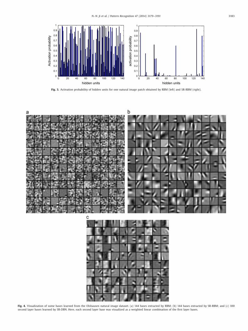
Fig. 4. Visualization of some bases learned from the Olshausen natural image dataset. (a) 144 bases extracted by RBM; (b) 144 bases extracted by SR-RBM; and (c) 100second layer bases learned by SR-DBN. Here, each second layer base was visualized as a weighted linear combination of the first layer bases.

0 20 40 60 80 100 120 1400

0.1

0.2

0.3

0.4

0.5

0.6

0.7

0.8

0.9

1

hidden units

Act

ivat

ion

prob

abili

ty

0 20 40 60 80 100 120 1400

0.1

0.2

0.3

0.4

0.5

0.6

0.7

0.8

0.9

1

hidden units

activ

atio

n pr

obab

ility

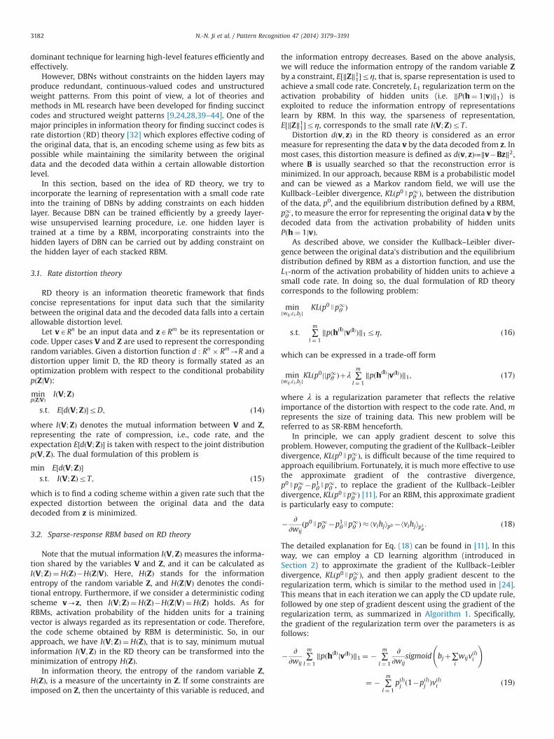
Fig. 3. Activation probability of hidden units for one natural image patch obtained by RBM (left) and SR-RBM (right).

N.-N. Ji et al. / Pattern Recognition 47 (2014) 3179–3191 3183

� ∂∂bj

∑m

l ¼ 1‖pðhðlÞjvðlÞÞ‖1 ¼ � ∑

m

l ¼ 1

∂∂bj

sigmoid bjþ∑iwijv

ðlÞi

!

¼ � ∑m

l ¼ 1pðlÞj ð1�pðlÞj Þ ð20Þ

where pðlÞj ¼ sigmoidð∑ivðlÞi wijþbjÞ, and sigmoidð�Þ stands for the

sigmoid function.In order to increase computational efficiency, in the gradient

step that tries to minimize the regularization term, we update onlythe bias terms bj's (which directly control the degree to which thehidden units are activated), instead of updating all the parametersbj and wij's.

Algorithm 1. SR-RBM learning algorithm.

1. Update the parameters using CD learning rule as follows:wij≔wijþϵð⟨vihj⟩p0 � ⟨vihj⟩p1

θÞ;

ci≔ciþϵð⟨vi⟩p0 � ⟨vi⟩p1θÞ;

bj≔bjþϵð⟨hj⟩p0 � ⟨hj⟩p1θÞ;

where ϵ is a learning rate, and ⟨ � ⟩p1θis an expectation over

the reconstruction data, estimated using one iteration ofGibbs sampling;

2. Update the parameters using the gradient of theregularization term by Eqs. (19) and (20);

3. Repeat Steps 1 and 2 until converge.

3.3. Learning deep belief network using SR-RBM

Similar to DBN's architecture, DBN based on the idea of RD theory,referred to as SR-DBN, is composed of several SR-RBMs. The corre-sponding learning algorithm is also greedy layer-by-layer. When thebottom SR-RBM is trained, the parameters wij, ci and bj are frozen andthe hidden unit values given the data are inferred by Eq. (5). Then,these inferred values serve as the “data” used to train the next higherlayer in the network, i.e. the next SR-RBM. This process can berepeated several times to learn a deep and hierarchical model.

4. Experiments

In this section, we carry out some experiments on four imagestimulus datasets (namely, natural images [32], MNIST dataset[45], NORB dataset [46] and CIFAR-10 dataset [47]) to evaluate andcompare the performance of our algorithm with that of severalother algorithms (i.e., PCA [48], RBM [10,11], DBN composed ofRBM [7], SparseRBM [24] and SparseDBN [24]) qualitatively andquantitatively. In all experiments, we initialized weights andbiases as some random numbers which come from a uniformdistribution. To speed-up the learning process, we divided eachdataset into mini-batches, and updated the weights after eachmini-batch. Moreover, we preprocessed each image patch bysubtracting the mean pixel value, and dividing the result by itsstandard deviation.

4.1. Natural image

We first tested our model's ability to learn hierarchical repre-sentations of natural images. Training data are a set of 12�12pixel natural image patches taken from ten 512�512 images ofnatural surroundings in the American northwest, made availableby Olshausen et. al [32]. We used 100,000 12�12 patchesrandomly sampled from these images, skipping over any patchwithin 1 pixel of the border of the image. Each subset of 200patches was used as a mini-batch.

First, we trained SR-RBM and RBM models with 144 visibleunits and 144 hidden units. Fig. 3 shows activation probability ofhidden units caused by one input data, i.e., representations of thisinput data obtained by RBM and SR-RBM. For other training data,representations obtained by these two models are similar to thoseillustrated in Fig. 3. From this figure, we can see that informationentropy of the representation obtained by SR-RBM is much smallerthan that obtained by RBM, because the values of most compo-nents of representation learnt by SR-RBM approximate to zeros(while the components corresponding to RBM spread over thewhole interval ð0;1Þ), which reduces uncertainty of the represen-tations obtained by SR-RBM over all training patterns.

Fig. 4(b) shows the learned bases corresponding to SR-RBM.It can be observed that they are oriented, gabor-like bases and

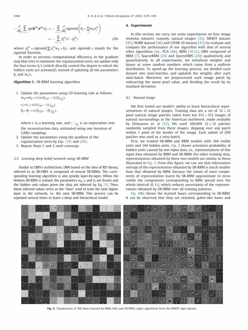
Fig. 5. Visualization of 196 bases learned by RBM (left) and SR-RBM (right) algorithms from the MNIST digit dataset.

N.-N. Ji et al. / Pattern Recognition 47 (2014) 3179–31913184

resemble the receptive fields of V1 simple cells. These results areconsistent with much previous work [3,9,24,32,49,50]. In contrast,the standard RBM results in bases that were neither oriented norlocalized, as shown in Fig. 4(a).

Thenwe learned a SR-DBN with two hidden layers by stacking oneSR-RBM on top of another, and 144 and 50 units were used in the firstand second hidden layers, respectively. The learned second layer baseswere visualized as weighted linear combination of the first layer bases,and were illustrated in Fig. 4(c). Note that this visualization methodwill also be used in next experiments. From Fig. 4(c), we can see thatmany bases responded selectively to contours, corners, angles, andsurface boundaries in the images. These results are qualitativelyconsistent with those reported in [24,51,52].

4.2. MNIST digit dataset

The MNIST digit dataset contains 60,000 training and 10,000test images of 10 handwritten digits (0–9), each image with size28�28 pixels [45]. In our experiments, to speed up the learningprocess, we sampled the first 2000 images per class to train ouralgorithm as well as other unsupervised feature extraction algo-rithms. The size of mini-batch was set to 200.

In order to qualitatively compare the bases obtained by SR-RBMand RBM, we first trained them with 784 visible units and 196hidden units. The learning rates for weights and biases were set to0.001. Although 196 is less than the input dimensionality of 784,the representation is still overcomplete because the effectivedimension of the digit dataset is considerably less than 784 aspointed out in [9]. Fig. 5 shows the resulted bases learnt by SR-RBM and RBM. It can be found that the majority of the bases learntby RBM appear to be local blob detectors, with only a few thatspecialize as little stroke detectors. Meanwhile, there were a fewbases remaining uninformative (i.e., almost uniform random greypatches). With SR-RBM, a much larger proportion of interesting

(visibly not random, blob detectors and with a clear structure)feature detectors were learnt. These include local oriented strokedetectors and detectors of digit parts such as loops. This result isconsistent with those obtained by applying different algorithms tolearn representations of this dataset [9,53]. The representations of

Table 1Error rate on MNIST training (with 100, 500 and 1000 samples per class) and testsets produced by a linear classifier trained on active probability of hidden unitsproduced by SparseRBM with several values of p, which is the target of sparsity ofSparseRBM. (λ is set to 2 which is chosen by try-and-error.)

p 100 Samples 500 Samples 1000 Samples

Trainingerrors

Testingerrors

Trainingerrors

Testingerrors

Trainingerrors

Testingerrors

0.005 0.07 10.34 2.86 4.91 3.53 4.600.01 0.06 9.98 2.80 4.92 3.49 4.510.02 0.05 9.17 2.68 4.64 3.33 4.410.03 0.05 9.44 2.69 4.84 3.51 4.56

Table 2Error rate on MNIST training (with 100, 500 and 1000 samples per class) and testsets produced by a linear classifier trained on active probability of hidden unitsproduced by SR-RBM with several values of λ.

λ 100 Samples 500 Samples 1000 Samples

Trainingerrors

Testingerrors

Trainingerrors

Testingerrors

Trainingerrors

Testingerrors

0.02 0.04 9.37 3.04 5.31 3.91 4.960.03 0.04 8.32 2.51 4.54 3.19 4.260.04 0.05 8.24 2.47 4.45 3.18 4.140.05 0.06 8.24 2.84 4.92 3.67 4.69

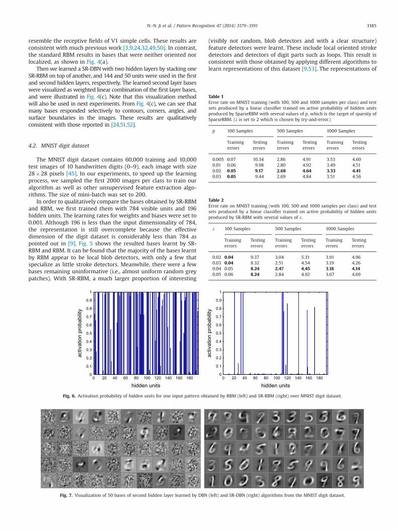
Fig. 7. Visualization of 50 bases of second hidden layer learned by DBN (left) and SR-DBN (right) algorithms from the MNIST digit dataset.

0 20 40 60 80 100 120 140 160 1800

0.1

0.2

0.3

0.4

0.5

0.6

0.7

0.8

0.9

1

hidden units

activ

atio

n pr

obab

ility

0 20 40 60 80 100 120 140 160 1800

0.1

0.2

0.3

0.4

0.5

0.6

0.7

0.8

0.9

1

hidden units

activ

atio

n pr

obab

ility

Fig. 6. Activation probability of hidden units for one input pattern obtained by RBM (left) and SR-RBM (right) over MNIST digit dataset.

N.-N. Ji et al. / Pattern Recognition 47 (2014) 3179–3191 3185

one input pattern learnt by RBM and SR-RBM models are shown inFig. 6.

Furthermore, in order to learn hierarchical features, we thentrained a second RBM and SR-RBM based on the activationprobability of hidden units produced by RBM and SR-RBM in theabove experiment. These stacked RBM and SR-RBM composed aDBN and a SR-DBN. Here, training was performed on 50 hidden

units and we decreased the code rate (increase the value of λ) forSR-DBN. The bases generated by the second hidden layer arevisualized in Fig. 7. These results indicate that the bases of thesecond hidden layer learnt by SR-DBN are more abstract thanthose obtained by DBN. It is obvious that they learned the digitsdistinctly. By contrast, the bases learnt by DBN remain uninterest-ing since they are almost uniform random grey patches. Therefore,SR-DBN is able to capture higher-order correlations among theinput pixel intensities.

100 200 300 4000

5

10

15

20

25

Number of hidden units

Err

or R

ate

100 samples

100 200 300 4002

4

6

8

10

12

14

16

Number of hidden units

Err

or R

ate

500 samples

100 200 300 4002

4

6

8

10

12

14

16

Number of hidden units

Err

or R

ate

1000 samples

RBML1: trainSparseRBM: trainPCA: trainRBML1: testSparseRBM: testPCA: test

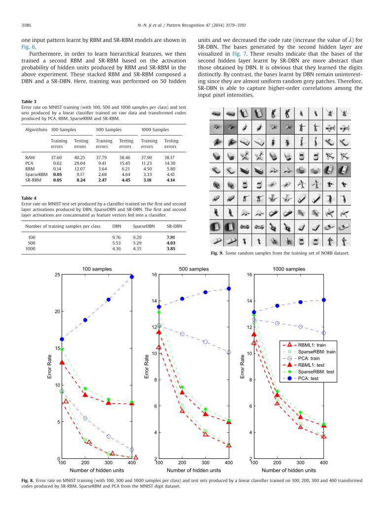
Fig. 8. Error rate on MNIST training (with 100, 500 and 1000 samples per class) and test sets produced by a linear classifier trained on 100, 200, 300 and 400 transformedcodes produced by SR-RBM, SparseRBM and PCA from the MNIST digit dataset.

Fig. 9. Some random samples from the training set of NORB dataset.

Table 4Error rate on MNIST test set produced by a classifier trained on the first and secondlayer activations produced by DBN, SparseDBN and SR-DBN. The first and secondlayer activations are concatenated as feature vectors fed into a classifier.

Number of training samples per class DBN SparseDBN SR-DBN

100 9.76 9.29 7.91500 5.53 5.29 4.03

1000 4.36 4.35 3.85

Table 3Error rate on MNIST training (with 100, 500 and 1000 samples per class) and testsets produced by a linear classifier trained on raw data and transformed codesproduced by PCA, RBM, SparseRBM and SR-RBM.

Algorithms 100 Samples 500 Samples 1000 Samples

Trainingerrors

Testingerrors

Trainingerrors

Testingerrors

Trainingerrors

Testingerrors

RAW 37.60 40.25 37.79 38.46 37.90 38.17PCA 0.62 29.04 9.41 15.45 11.23 14.30RBM 0.14 12.07 3.64 6.21 4.50 5.80SparseRBM 0.05 9.17 2.68 4.64 3.33 4.41SR-RBM 0.05 8.24 2.47 4.45 3.18 4.14

N.-N. Ji et al. / Pattern Recognition 47 (2014) 3179–31913186

To empirically verify the advantage of the representation learntby SR-RBM in terms of its discriminative power, we first executedSR-RBM and several other unsupervised feature extraction algo-rithms (i.e., PCA, RBM and SparseRBM) on 20,000 images (i.e. 2000images per class), then used their created representations as inputfor the same linear classifier. The number of hidden units for RBM,SparseRBM and SR-RBM was set to 500, and the number ofprincipal components for PCA was also set to 500. For theclassification process, we used representations of 100, 500 and1000 images per class to train a linear classifier. The representa-tions of remaining images were used for test. For each combina-tion of training data size and algorithm, we trained 50 classifierswith randomly chosen training sets and then used the averageclassification error to evaluate the performance of the correspond-ing algorithm. Note that SparseRBM and SR-RBM involve somehyper-parameter (i.e., λ and p for SparseRBM, λ for SR-RBM,the detailed algorithm of SparseRBM can be found in [24]),we took several values of these hyper-parameters to conductexperiments.

Table 1 displays the training and test error rates of a linearclassifier when providing the representations generated by aSparseRBM as its input. Table 2 reports the results for SR-RBM.In order to facilitate the comparison, the best results were high-lighted in bold. When compared with PCA and RBM, we chosenthe best results of SparseRBM and SR-RBM under each trainingsample size. In addition, the recognition ability based on raw datawas also considered. These comparison results were displayed in

Table 3. From Table 3, we can see that SR-RBM always achieves thebest recognition accuracy on the training and test sets when usinga different number of training samples. Furthermore, in order tocompare the representations learnt by DBN, SparseDBN and SR-DBN in terms of their discriminative power, we trained RBM,SparseRBM and SR-RBM with 100 hidden units again, by consider-ing the representations learnt by RBM, SparseRBM and SR-RBMmentioned above as visible data. We constructed representationfor each image by concatenating the first and second layeractivations, and trained the same classifier using these representa-tions. Table 4 displays the error rate on the test set.

Moreover, recognition ability of hidden representations whenthrowing out those units whose activation times were lower thana threshold was also tested. Specifically, we trained linear classi-fiers on the activation probabilities of 100, 200, 300 and 400hidden units among 500 units. These hidden units were activatedby the most input images. For each algorithm (i.e., SR-RBM,SparseRBM and PCA), Fig. 8 plots the training and test error ratesof a linear classifier as a function of the number of hidden units.From this figure, SR-RBM is seen to learn more discriminativehidden representations than SparseRBM and PCA. This advantageis more noticeable for small training datasets.

4.3. NORB dataset

NORB [46] is a considerably more difficult dataset than MNIST,which contains images of 50 different 3D toy objects with 10objects in each of five generic classes: cars, trucks, planes, animalsand humans. Each object is captured from different viewpointsand under various lighting conditions. The training set contains24,300 stereo image pairs of 25 objects, 5 per class, while the testset contains 24,300 stereo pairs of the remaining, different 25objects. Considering the computational cost, we subsampled theoriginal 2�108�108 stere-pair images to 2�32�32, and ran-domly sampled 10,000 images from the training set to train ouralgorithm and other unsupervised feature extraction algorithms.The size of mini-batch was set to 100. Some random samples usedin our experiments are shown in Fig. 9.

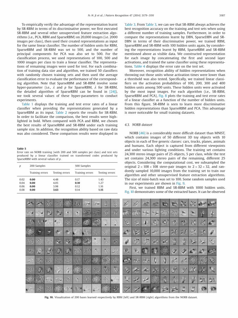
First, we trained RBM and SR-RBM with 1000 hidden units.Fig. 10 demonstrates some of the extracted bases. It can be observed

Fig. 10. Visualization of 200 bases learned respectively by RBM (left) and SR-RBM (right) algorithms from the NORB dataset.

Table 5Error rate on NORB training (with 200 and 500 samples per class) and test setsproduced by a linear classifier trained on transformed codes produced bySparseRBM with several values of p.

p 200 Samples 500 Samples

Training errors Testing errors Training errors Testing errors

0.02 0.00 4.48 0.17 1.430.04 0.00 4.05 0.10 1.270.06 0.00 3.98 0.12 1.160.08 0.00 3.63 0.14 1.15

N.-N. Ji et al. / Pattern Recognition 47 (2014) 3179–3191 3187

that most bases obtained by SR-RBM appear to be object-partdetectors and contour detectors. As for RBM, the majority of thebases appear to be local blob detectors and edge detectors, withonly a few that specialized as contour detectors. Therefore, SR-RBMis able to learn features that are more attractive.

In order to test the discriminative power of the representationslearnt by SR-RBM, it was compared with representations learnt byRBM, SparseRBM and PCA. Similar to the experiment done withthe MNIST dataset, we chose 200 and 500 samples per class astraining set size. For each combination of training data size andalgorithm, we trained 50 classifiers with randomly chosen trainingsets and then used the average classification error to evaluate theperformance of the corresponding algorithm. Table 5 displays thetraining and test error rates of a linear classifier when providingthe representations generated by a SparseRBM as its input. Table 6reports the results for SR-RBM. We chose the best results tocompare with RBM and PCA, as shown in Table 7. From this table,SR-RBM achieves the best recognition accuracy on the training andtest sets when using a different number of training samples.Furthermore, the discriminative power of the representationslearnt by DBN, SparseDBN and SR-DBN were also compared.Similar to MNIST, we then trained a second RBM, SparseRBMand SR-RBM to obtain the corresponding DBN, SparseDBN andSR-DBN, and constructed representations of images by concatenatingthe first and second layer activation probabilities. Table 8 displaysthe error rate on the test set obtained by using these representa-tions for classification.

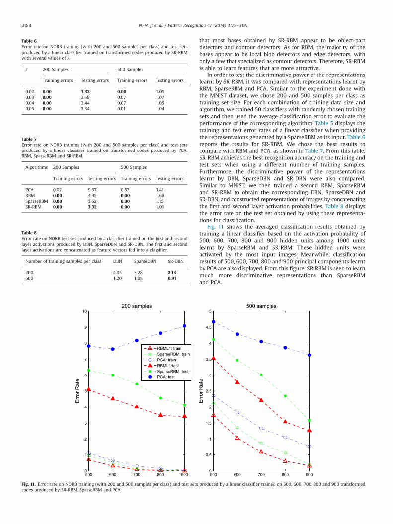
Fig. 11 shows the averaged classification results obtained bytraining a linear classifier based on the activation probability of500, 600, 700, 800 and 900 hidden units among 1000 unitslearnt by SparseRBM and SR-RBM. These hidden units wereactivated by the most input images. Meanwhile, classificationresults of 500, 600, 700, 800 and 900 principal components learntby PCA are also displayed. From this figure, SR-RBM is seen to learnmuch more discriminative representations than SparseRBMand PCA.

Table 8Error rate on NORB test set produced by a classifier trained on the first and secondlayer activations produced by DBN, SparseDBN and SR-DBN. The first and secondlayer activations are concatenated as feature vectors fed into a classifier.

Number of training samples per class DBN SparseDBN SR-DBN

200 4.05 3.28 2.13500 1.20 1.08 0.91

500 600 700 800 9000

1

2

3

4

5

6

7

8

9

10

Err

or R

ate

200 samples

500 600 700 800 9000

0.5

1

1.5

2

2.5

3

3.5

4

4.5

5

Err

or R

ate

500 samples

RBML1: trainSparseRBM: trainPCA: trainRBML1:testSparseRBM: testPCA: test

Fig. 11. Error rate on NORB training (with 200 and 500 samples per class) and test sets produced by a linear classifier trained on 500, 600, 700, 800 and 900 transformedcodes produced by SR-RBM, SparseRBM and PCA.

Table 7Error rate on NORB training (with 200 and 500 samples per class) and test setsproduced by a linear classifier trained on transformed codes produced by PCA,RBM, SparseRBM and SR-RBM.

Algorithms 200 Samples 500 Samples

Training errors Testing errors Training errors Testing errors

PCA 0.02 9.67 0.57 3.41RBM 0.00 4.95 0.00 1.68SparseRBM 0.00 3.62 0.00 1.15SR-RBM 0.00 3.32 0.00 1.01

Table 6Error rate on NORB training (with 200 and 500 samples per class) and test setsproduced by a linear classifier trained on transformed codes produced by SR-RBMwith several values of λ.

λ 200 Samples 500 Samples

Training errors Testing errors Training errors Testing errors

0.02 0.00 3.32 0.00 1.010.03 0.00 3.59 0.07 1.070.04 0.00 3.44 0.07 1.050.05 0.00 3.34 0.01 1.04

N.-N. Ji et al. / Pattern Recognition 47 (2014) 3179–31913188

4.4. CIFAR-10 dataset

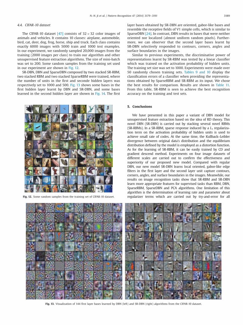
The CIFAR-10 dataset [47] consists of 32�32 color images ofanimals and vehicles. It contains 10 classes: airplane, automobile,bird, cat, deer, dog, frog, horse, ship and truck. Each class containsexactly 6000 images with 5000 train and 1000 test examples.In our experiment, we randomly sampled 20,000 images from thetraining (2000 images per class) to train our algorithm and otherunsupervised feature extraction algorithms. The size of mini-batchwas set to 200. Some random samples from the training set usedin our experiment are shown in Fig. 12.

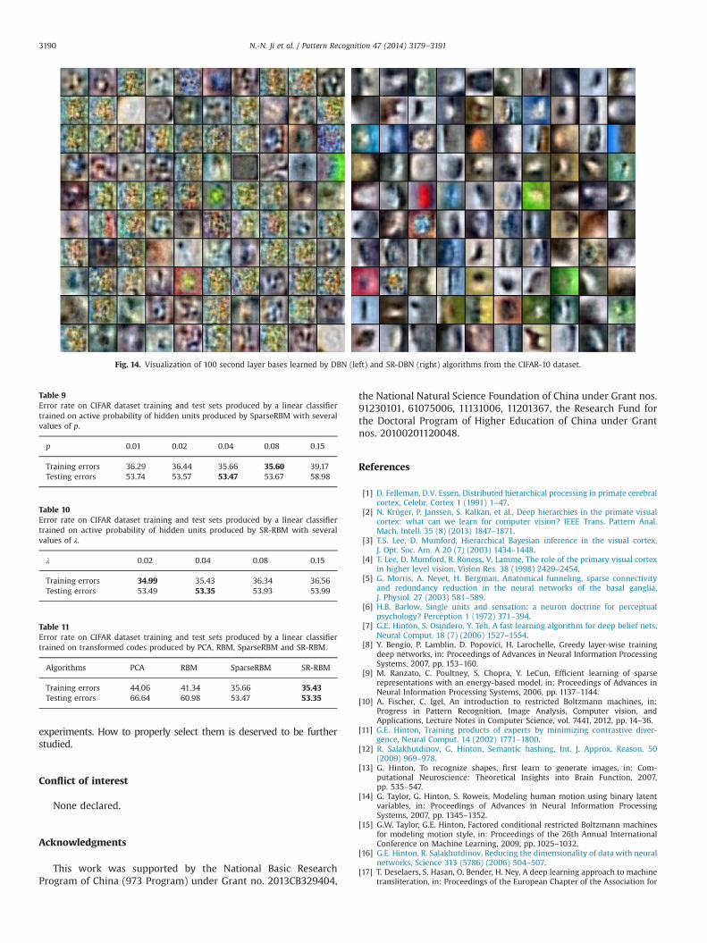
SR-DBN, DBN and SparseDBN composed by two stacked SR-RBM,two stacked RBM and two stacked SparseRBM were trained, wherethe number of units in the first and seconde hidden layers wasrespectively set to 1000 and 500. Fig. 13 shows some bases in thefirst hidden layer learnt by DBN and SR-DBN, and some baseslearned in the second hidden layer are shown in Fig. 14. The first

layer bases obtained by SR-DBN are oriented, gabor-like bases andresemble the receptive fields of V1 simple cells, which is similar toSparseDBN [24]. In contrast, DBN results in bases that were neitheroriented nor localized (almost uniform random pixels). Further-more, we can observer that the second layer bases learnt bySR-DBN selectively responded to contours, corners, angles andsurface boundaries in the images.

Similar to previous experiments, the discriminative power ofrepresentations learnt by SR-RBM was tested by a linear classifierwhich was trained on the activation probability of hidden units.The training set size was set to 1000. Experiments were made over50 randomly chosen training sets. Tables 9 and 10 display theclassification errors of a classifier when providing the representa-tions obtained by SparseRBM and SR-RBM as its input. We chosethe best results for comparison. Results are shown in Table 11.From this table, SR-RBM is seen to achieve the best recognitionaccuracy on the training and test sets.

5. Conclusions

We have presented in this paper a variant of DBN model forunsupervised feature extraction based on the idea of RD theory. Thisnovel DBN (SR-DBN) is carried out by stacking several novel RBMs(SR-RBMs). In a SR-RBM, sparse response induced by a L1 regulariza-tion term on the activation probability of hidden units is used toachieve small rate of codes. At the same time, the Kullback–Leiblerdivergence between original data's distribution and the equilibriumdistribution defined by the model is employed as a distortion function.As for the learning of SR-RBM, it can be easily trained by CD andgradient descend method. Experiments on four image datasets ofdifferent scales are carried out to confirm the effectiveness andsuperiority of our proposed new model. Compared with regularDBN, our new model SR-DBN learns local oriented, gabor-like edgefilters in the first layer and the second layer unit capture contours,corners, angles, and surface boundaries in the images. Meanwhile, ourresults on image recognition tasks show that SR-RBM and SR-DBNlearn more appropriate features for supervised tasks than RBM, DBN,SparseRBM, SparseDBN and PCA algorithms. One limitation of thisalgorithm is the determination of learning rate and parameter aboutregularizer terms which are carried out by try-and-error for allFig. 12. Some random samples from the training set of CIFAR-10 dataset.

Fig. 13. Visualization of 144 first layer bases learned by DBN (left) and SR-DBN (right) algorithms from the CIFAR-10 dataset.

N.-N. Ji et al. / Pattern Recognition 47 (2014) 3179–3191 3189

experiments. How to properly select them is deserved to be furtherstudied.

Conflict of interest

None declared.

Acknowledgments

This work was supported by the National Basic ResearchProgram of China (973 Program) under Grant no. 2013CB329404,

the National Natural Science Foundation of China under Grant nos.91230101, 61075006, 11131006, 11201367, the Research Fund forthe Doctoral Program of Higher Education of China under Grantnos. 20100201120048.

References

[1] D. Felleman, D.V. Essen, Distributed hierarchical processing in primate cerebralcortex, Celebr. Cortex 1 (1991) 1–47.

[2] N. Krüger, P. Janssen, S. Kalkan, et al., Deep hierarchies in the primate visualcortex: what can we learn for computer vision? IEEE Trans. Pattern Anal.Mach. Intell. 35 (8) (2013) 1847–1871.

[3] T.S. Lee, D. Mumford, Hierarchical Bayesian inference in the visual cortex,J. Opt. Soc. Am. A 20 (7) (2003) 1434–1448.

[4] T. Lee, D. Mumford, R. Roness, V. Lamme, The role of the primary visual cortexin higher level vision, Vision Res. 38 (1998) 2429–2454.

[5] G. Morris, A. Nevet, H. Bergman, Anatomical funneling, sparse connectivityand redundancy reduction in the neural networks of the basal ganglia,J. Physiol. 27 (2003) 581–589.

[6] H.B. Barlow, Single units and sensation: a neuron doctrine for perceptualpsychology? Perception 1 (1972) 371–394.

[7] G.E. Hinton, S. Osindero, Y. Teh, A fast learning algorithm for deep belief nets,Neural Comput. 18 (7) (2006) 1527–1554.

[8] Y. Bengio, P. Lamblin, D. Popovici, H. Larochelle, Greedy layer-wise trainingdeep networks, in: Proceedings of Advances in Neural Information ProcessingSystems, 2007, pp. 153–160.

[9] M. Ranzato, C. Poultney, S. Chopra, Y. LeCun, Efficient learning of sparserepresentations with an energy-based model, in: Proceedings of Advances inNeural Information Processing Systems, 2006, pp. 1137–1144.

[10] A. Fischer, C. Igel, An introduction to restricted Boltzmann machines, in:Progress in Pattern Recognition, Image Analysis, Computer vision, andApplications, Lecture Notes in Computer Science, vol. 7441, 2012, pp. 14–36.

[11] G.E. Hinton, Training products of experts by minimizing contrastive diver-gence, Neural Comput. 14 (2002) 1771–1800.

[12] R. Salakhutdinov, G. Hinton, Semantic hashing, Int. J. Approx. Reason. 50(2009) 969–978.

[13] G. Hinton, To recognize shapes, first learn to generate images, in: Com-putational Neuroscience: Theoretical Insights into Brain Function, 2007,pp. 535–547.

[14] G. Taylor, G. Hinton, S. Roweis, Modeling human motion using binary latentvariables, in: Proceedings of Advances in Neural Information ProcessingSystems, 2007, pp. 1345–1352.

[15] G.W. Taylor, G.E. Hinton, Factored conditional restricted Boltzmann machinesfor modeling motion style, in: Proceedings of the 26th Annual InternationalConference on Machine Learning, 2009, pp. 1025–1032.

[16] G.E. Hinton, R. Salakhutdinov, Reducing the dimensionality of data with neuralnetworks, Science 313 (5786) (2006) 504–507.

[17] T. Deselaers, S. Hasan, O. Bender, H. Ney, A deep learning approach to machinetransliteration, in: Proceedings of the European Chapter of the Association for

Fig. 14. Visualization of 100 second layer bases learned by DBN (left) and SR-DBN (right) algorithms from the CIFAR-10 dataset.

Table 9Error rate on CIFAR dataset training and test sets produced by a linear classifiertrained on active probability of hidden units produced by SparseRBM with severalvalues of p.

p 0.01 0.02 0.04 0.08 0.15

Training errors 36.29 36.44 35.66 35.60 39.17Testing errors 53.74 53.57 53.47 53.67 58.98

Table 10Error rate on CIFAR dataset training and test sets produced by a linear classifiertrained on active probability of hidden units produced by SR-RBM with severalvalues of λ.

λ 0.02 0.04 0.08 0.15

Training errors 34.99 35.43 36.34 36.56Testing errors 53.49 53.35 53.93 53.99

Table 11Error rate on CIFAR dataset training and test sets produced by a linear classifiertrained on transformed codes produced by PCA, RBM, SparseRBM and SR-RBM.

Algorithms PCA RBM SparseRBM SR-RBM

Training errors 44.06 41.34 35.66 35.43Testing errors 66.64 60.98 53.47 53.35

N.-N. Ji et al. / Pattern Recognition 47 (2014) 3179–31913190

Computational Linguistics Workshop on Statistical Machine Translation, 2009,pp. 233–241.

[18] A. Mohamed, G. Dahl, G. Hinton, Deep belief networks for phone recognition,in: Proceedings of Advances in Neural Information Processing Systems Work-shop Deep Learning for Speech Recognition and Related Application, 2009.

[19] G. Dahl, G.E. Hionton, Acoustic modeling using deep belief networks, IEEETrans. Audio Speech Lang. Process. 20 (2012) 14–22.

[20] G. Hinton, L. Deng, D. Yu, et al., Deep neural networks for acoustic modeling inspeech recognition: the Shared Views of Four Research Groups, IEEE SignalProcess. Mag. 29 (6) (2012) 82–97.

[21] E. Horster, R. Lienhart, Deep networks for image retrieval on large-scaledatabases, in: Proceedings of the 16th ACM International Conference onMultimedia, ACM, Vancouver British Columbia, Canada, 2008, pp. 643–646.

[22] E. Chen, X. Yang, H. Zha, R. Zhang, W. Zhang, Learning object classes fromimage thumbnails through deep neural networks, in: Proceedings of theInternational Conference on Acoustics, Speech and Signal Processing, 2008,pp. 829–832.

[23] Y. Liu, S. Zhou, Q.C. Chen, Discriminative deep belief networks for visual dataclassification, Pattern Recognit. 44 (10) (2011) 2287–2296.

[24] H. Lee, C. Ekanadham, A. Ng, Sparse deep belief net model for visual area V2,in: Proceedings of Advances in Neural Information Processing Systems, 2007,pp. 1416–1423.

[25] R. Salakhutdinov, I. Murray, On the quantitative analysis of deep beliefnetworks, in: Proceedings of the International Conference on Machine Learn-ing, ACM, Helsinki, Finland, 2008, pp. 872–879.

[26] P. Vincent, H. Larochelle, Y. Bengio, P. Manzagol, Extracting and composingrobust features with denoising autoencoders, in: Proceedings of the Interna-tional Conference on Machine Learning, ACM, Helsinki, Finland, 2008,pp. 1096–1103.

[27] R. Raina, A. Madhavan, A. Ng, Large-scale deep unsupervised learning usinggraphics processors, in: Proceedings of the International Conference onMachine Learning, ACM, Canada, 2009, pp. 873–880.

[28] M. Ranzato, Y.L. Boureau, Y. LeCun, Sparse feature learning for deep beliefnetworks, in: Proceedings of Advances in Neural Information ProcessingSystems, 2008, pp. 1185–1192.

[29] H. Luo, R. Shen, C. Niu, C. Ullrich, Sparse group restricted Boltzmann machines,in: Proceedings of the 25th AAAI Conference on Artificial Intelligence (AAAI),2011.

[30] X. Halkias, S. Paris, H. Glotin, Sparse Penalty in Deep Belief Networks: Usingthe Mixed Norm Constraint, ⟨http://arxiv.org/abs/1301.3533⟩.

[31] B. Olshausen, D. Field, Emergence of simple-cell receptive field properties bylearning sparse code for natural images, Nature (1996) 607–609.

[32] T.M. Cover, J.A. Thomas, Elements of Information Theory, 2nd ed., Wiley-InterScience, Hoboken, NJ, 2006.

[33] H. Hino, M. Noboru, An information theoretic perspective of the sparse coding,Advances in Neural Networks, Springer, Berlin, Heidelberg, 2009, pp. 84–93.

[34] S. Hochreiter, J. Schmidhuber, Low-complexity coding and decoding, in:Theoretical Aspects of Neural Computation (TANC 97), Hong Kong, 1997,pp. 297–306.

[35] P. Smolensky, Information processing in dynamical systems: foundations ofharmony theory, in: D.E. Rumelhart, J.L. McClelland (Eds.), Parallel DistributedProcessing, vol. 1, MIT Press, Cambridge, MA, 1986, pp. 194–281.

[36] Y. Freund, D. Haussler, Unsupervised learning of distributions on binaryvectors using two layer networks, in: Proceedings of Advances in NeuralInformation Processing Systems, 1992, pp. 912–919.

[37] G.E. Hinton, A Practical Guide to Training Restricted Boltzmann Machines,Machine Learning Group, University of Toronto, Toronto, ON, Canada, Techni-cal Report 2010-003, 2010.

[38] Y. Bengio, Learning deep architectures for AI, Found. Trends Mach. Learn. 2 (1)(2009) 1–127.

[39] B. Olshausen, D. Field, Sparse coding with an overcomplete basis set:a strategy employed by V1? Vision Res. 37 (1997) 3311–3325.

[40] O. Shamir, S. Sabato, N. Tishby, Learning and generalization with theinformation bottleneck, Theor. Comput. Sci. 411 (2010) 2696–2711.

[41] L. Buesing, M. Wolfgang, Simplified rules and theoretical analysis for informa-tion bottleneck optimization and PCA with spiking neurons, in: Advances inNeural Information Processing Systems, vol. 20, 2007, pp. 193–200.

[42] J.F.M. Jehee, C. Rothkopf, J.M. Beck, et al., Learning receptive fields usingpredictive feedback, J. Physiol. Paris 100.1 (2006) 125–132.

[43] C. Plahl, T.N. Sainath, B. Ramabhadran, D. Nahamoo, Improved pre-training ofdeep belief networks using sparse encoding symmetric machines, in: Pro-ceedings of the International Conference on Acoustics, Speech, and SignalProcessing, 2012, pp. 4156–4168.

[44] T.N. Sainath, B. Kingsbury, B. Ramabhadran, Auto-encoder bottleneck featuresusing deep belief networks, in: Proceedings of the International Conference onAcoustics, Speech, and Signal Processing, 2012, pp. 4153-4156.

[45] The MNIST Database of Handwritten Digits, ⟨http://yann.lecun.com/exdb/mnist/⟩.

[46] Y. LeCun, F. Huang, L. Bottou, Learning methods for generic object recognitionwith invariance to pose and lighting, in: IEEE Conference on Computer Visionand Pattern Recognition, vol. 2, 2004, pp. 97–104.

[47] A. Krizhevsky, G.E. Hinton, Learning Multiple Layers of Features from TinyImages, Technical Report, University of Toronto, 2009.

[48] I.T. Jolliffe, Principal Component Analysis, vol. 487, Springer-Verlag, New York,1986.

[49] A.J. Bell, T.J. Sejnowski, The ‘independent components’ of natural scenes areedge filters, Vision Res. 37 (23) (1997) 3327–3338.

[50] S. Osindero, M. Welling, G.E. Hinton, Topographic product models applied tonatural scene statistics, Neural Comput. 18 (2) (2006) 381–344.

[51] A. Hyvärinen, M. Gutmann, P.O. Hoyer, Statistical model of natural stimulipredicts edge-like pooling of spatial frequency channels in V2, BMC Neurosci.6 (1) (2005) 12.

[52] M. Ito, H. Komatsu, Representation of angles embedded within contour stimuliin area V2 of macaque monkeys, J. Neurosci. 24 (13) (2004) 3313–3324.

[53] G.E. Hinton, S. Osindero, K. Bao, Learning causally linked MRFs, in: Interna-tional Conference on Artificial Intelligence and Statistics, 2005.

Nan-Nan Ji received the B.S. degree and the M.S. degree in Applied Mathematics from Chang'an University, Xi'an, China. She is currently a Ph.D. candidate with School ofMathematics and Statistics, Xi'an Jiaotong University. Her research interests are focused on neural network, deep learning, pattern recognition, and intelligence computation.

Jiang-She Zhang was born in 1962, and received his M.S. and Ph.D. degrees in Applied Mathematics from Xi'an Jiaotong University, Xi'an, China, in 1987 and 1993respectively. He joined Xi'an Jiaotong University, China, in 1987, where he is currently a full Professor in School of Mathematics and Statistics. Up to now, he has authored andcoauthored on monograph and over 50 journal papers on robust clustering, optimization, and short-term load forecasting for electric power system. His current researchfocus is on Bayesian learning, global optimization, ensemble learning, and deep learning.

Chun-Xia Zhang was born in 1980 and received her B.S. degree in Mathematics from Xinyang Normal University, Xinyang, China, in 2002. In 2005 and 2010, she received herM.S. and Ph.D. degrees respectively in Probability and Statistics, Applied Mathematics from Xian Jiaotong University, Xian, China. Currently, she is a Lecturer in School ofMathematics and Statistics at Xian Jiaotong University, China. She has published about 20 journal papers on ensemble learning techniques, and nonparametric regression.Her current research interests mainly include classifier combination strategies, bootstrap methods and deep learning.

N.-N. Ji et al. / Pattern Recognition 47 (2014) 3179–3191 3191