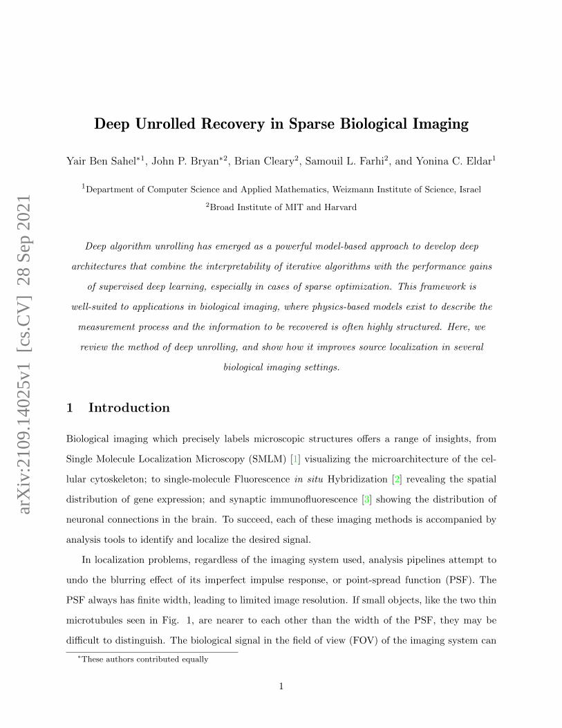
Deep Unrolled Recovery in Sparse Biological Imaging

Yair Ben Sahel∗1, John P. Bryan∗2, Brian Cleary2, Samouil L. Farhi2, and Yonina C. Eldar1

1Department of Computer Science and Applied Mathematics, Weizmann Institute of Science, Israel

2Broad Institute of MIT and Harvard

Deep algorithm unrolling has emerged as a powerful model-based approach to develop deep

architectures that combine the interpretability of iterative algorithms with the performance gains

of supervised deep learning, especially in cases of sparse optimization. This framework is

well-suited to applications in biological imaging, where physics-based models exist to describe the

measurement process and the information to be recovered is often highly structured. Here, we

review the method of deep unrolling, and show how it improves source localization in several

biological imaging settings.

1 Introduction

Biological imaging which precisely labels microscopic structures offers a range of insights, from

Single Molecule Localization Microscopy (SMLM) [1] visualizing the microarchitecture of the cel-

lular cytoskeleton; to single-molecule Fluorescence in situ Hybridization [2] revealing the spatial

distribution of gene expression; and synaptic immunofluorescence [3] showing the distribution of

neuronal connections in the brain. To succeed, each of these imaging methods is accompanied by

analysis tools to identify and localize the desired signal.

In localization problems, regardless of the imaging system used, analysis pipelines attempt to

undo the blurring effect of its imperfect impulse response, or point-spread function (PSF). The

PSF always has finite width, leading to limited image resolution. If small objects, like the two thin

microtubules seen in Fig. 1, are nearer to each other than the width of the PSF, they may be

difficult to distinguish. The biological signal in the field of view (FOV) of the imaging system can

∗These authors contributed equally

1

arX

iv:2

109.

1402

5v1

[cs

.CV

] 2

8 Se

p 20

21

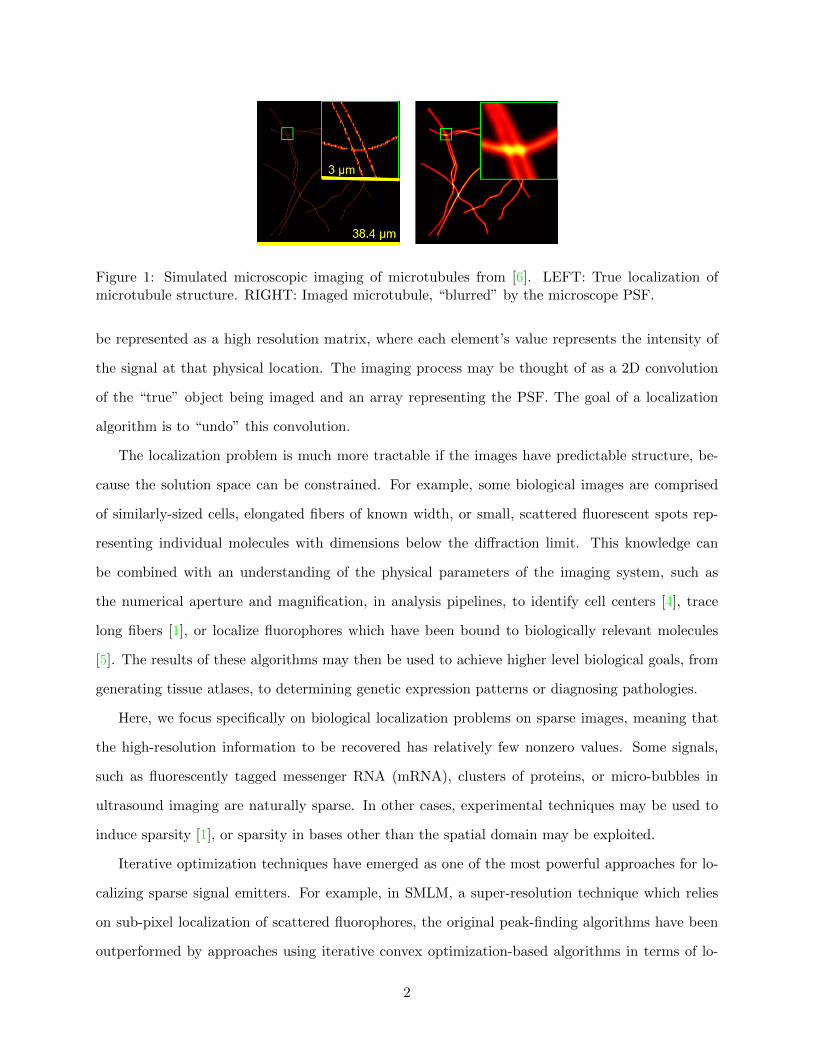
Figure 1: Simulated microscopic imaging of microtubules from [6]. LEFT: True localization ofmicrotubule structure. RIGHT: Imaged microtubule, “blurred” by the microscope PSF.

be represented as a high resolution matrix, where each element’s value represents the intensity of

the signal at that physical location. The imaging process may be thought of as a 2D convolution

of the “true” object being imaged and an array representing the PSF. The goal of a localization

algorithm is to “undo” this convolution.

The localization problem is much more tractable if the images have predictable structure, be-

cause the solution space can be constrained. For example, some biological images are comprised

of similarly-sized cells, elongated fibers of known width, or small, scattered fluorescent spots rep-

resenting individual molecules with dimensions below the diffraction limit. This knowledge can

be combined with an understanding of the physical parameters of the imaging system, such as

the numerical aperture and magnification, in analysis pipelines, to identify cell centers [4], trace

long fibers [1], or localize fluorophores which have been bound to biologically relevant molecules

[5]. The results of these algorithms may then be used to achieve higher level biological goals, from

generating tissue atlases, to determining genetic expression patterns or diagnosing pathologies.

Here, we focus specifically on biological localization problems on sparse images, meaning that

the high-resolution information to be recovered has relatively few nonzero values. Some signals,

such as fluorescently tagged messenger RNA (mRNA), clusters of proteins, or micro-bubbles in

ultrasound imaging are naturally sparse. In other cases, experimental techniques may be used to

induce sparsity [1], or sparsity in bases other than the spatial domain may be exploited.

Iterative optimization techniques have emerged as one of the most powerful approaches for lo-

calizing sparse signal emitters. For example, in SMLM, a super-resolution technique which relies

on sub-pixel localization of scattered fluorophores, the original peak-finding algorithms have been

outperformed by approaches using iterative convex optimization-based algorithms in terms of lo-

2

calization accuracy, signal-to-noise ratio (SNR), and resolution [7]. These advantages of iterative

optimization techniques for sparse recovery go beyond SMLM to other biological imaging problems,

providing high-accuracy localization in many settings [8][9][10]. However, they also suffer some dis-

advantages. They require adjustment of optimization parameters and explicit knowledge of the

impulse response of the imaging system, which restricts their use when the imaging system is not

well-characterized. They are computationally expensive and converge slowly, which limits their use

in real-time, live-cell imaging. Finally, they are relatively inflexible: a given algorithm is designed

to take advantage of a particular structure (here, signal sparsity), but ignores other context which

may be important (e.g., cell size or density).

Many of these disadvantages can be overcome by replacing the iterations of these algorithms

with trained neural networks which perform the same mathematical operation, a process known as

algorithmic unrolling [11] (alternatively, “unfolding”). By doing so, parameters which would have to

be specified explicitly or tuned empirically are learned automatically, and relevant context ignored

by the algorithm may be incorporated into the learned model. Since its introduction a decade ago,

a wide variety of techniques have been adapted using learned unrolling, enabling improvements in

performance across a variety of settings [12].

In the rest of this paper, we review how learned unrolling is applied to the localization of

sparse sources in biological imaging data. We first formulate biological localization as a sparse

recovery problem, and discuss the advantages and disadvantages of iterative approaches to sparse

recovery. We then describe how algorithmic unrolling addresses some of the shortcomings, and

how the general sparse recovery problem may be adapted to the unrolling framework. Next we

show in detail how unrolling has been used to achieve fast, accurate super-resolution in the optical

microscopy technique SMLM. We then turn to review a number of additional biological imag-

ing analysis problems to which unrolling has been applied to improve performance: Ultrasound

Localization Microscopy (ULM), Light-Field Microscopy (LFM), and cell center localization in flu-

orescence microscopy. Throughout, we discuss a number of additional data analysis problems in

sparse optical microscopy, and propose that algorithmic unrolling be applied, to achieve the same

benefits obtained in the reviewed techniques.

3

2 Sparse Recovery in Biological Imaging

The localization of biological objects, from microtubules to neural synapses, can be approached

effectively as a convex optimization problem. For ease of notation, we first reframe the imaging pro-

cess, typically thought of as a convolution, as a matrix-vector multiplication. The high-resolution

signal is “vectorized” and then multiplied by a matrix representing the PSF. We note that the prob-

lem can be formulated and solved with 2D convolutions equally well, and the techniques described

throughout the paper may be applied to a 2D formulation, as in [6] and [10].

Formally, we consider the FOV as a high-resolution square grid with side length nh. The total

number of locations in this grid is Nh = n2h. This grid is “vectorized” to form a vector x ∈ RNh . The

locations of emitters in the sample may be modeled by assigning each element of x a value related

to the number of photons emitted from that location within the FOV. If the FOV is imaged using

a sensor with Nl pixels (with Nh > Nl), then we can model the imaging process as multiplication

by a matrix A ∈ RNl×Nh , in which element (i, j) is the proportion of signal emitted from location j

on the high-resolution grid that will be detected at pixel i of the sensor. Thus defined, the columns

of A represent the PSF of the imaging system, such that column j of A is the PSF of the system

for a point source at location j. The (vectorized) measured image is then y = Ax, with y ∈ RNl .

The goal of the analysis pipeline is to infer the value of x, given y and A.

This inference problem can be formulated as a least-squares optimization problem: we seek to

find

x = arg minx

‖y −Ax‖22. (1)

Even if A is known perfectly, as long as Nh > Nl, A will have a nontrivial null space, so that the

optimization problem is underdetermined. Leveraging knowledge of the biological structure of x

can resolve this issue. If, as discussed above, it is known that x is sparse, then we may choose a

sparse optimization technique, such as the well-known LASSO [13], to recover x:

x = arg minx

‖y −Ax‖22 + λ‖x‖1. (2)

In particular, by correctly tuning λ, the minimizer x of (2) will provide accurate locations of each

signal-emitting object in the FOV.

4

3 Algorithmic Unrolling for Sparse Localization

Once a problem is framed as a sparse optimization of the form (2), a number of algorithms may be

used to find the minimizer x. Examples include the Alternating Direction Method of Multipliers

(ADMM), [14] the Iterative Shrinkage-Thresholding Algorithm (ISTA) [15], and the Half-Quadratic

Splitting algorithm (HQS)[16]. These methods converge to the correct minimizer x, but have some

limiting disadvantages, as discussed above: slow convergence, the requirement of parameters tuning

and explicit knowledge of the imaging system [6], and mathematical inflexibility.

Deep learning approaches have overcome some of these disadvantages. In analysis of SMLM

data, convolutional neural network models have achieved fast, accurate super-resolution [17], able

to improve recovery by incorporating structures not specified by the user. Deep learning, however,

comes with disadvantages of its own. In particular, deep learning is typically thought of as a

“black box” process: it is difficult to interpret the way the model transforms input to obtain a

result. Because of this, when inaccurate results are produced, it can be difficult to understand how

to improve the model. Typical deep learning approaches are strongly dependent on the available

training data, causing a lack of model robustness to new examples. Finally, when using generic

network architectures, many layers and parameters are typically required for good performance.

In 2010, Gregor and LeCun proposed a method to create neural networks based on iterative

methods used for sparse recovery [11], known as algorithm unrolling. The goal is to take advantage

of both the interpretability of iterative techniques and the flexibility of learned methods. In learned

unrolling, the transformation applied to the input by each iteration of the algorithm is replaced with

a neural network layer which applies the same type of function: for instance, matrix multiplication

can be replaced by a fully-connected layer, and thresholding can be replaced by an activation

function representing an appropriate regularizer. These iteration-layers are concatenated together,

and the resulting model-based neural network is optimized using supervised learning, with training

data consisting of paired examples of the signal vector x and measurement vector y from (2).

Training data may be obtained, for example, from measurement simulations with known ground

truth as in [6]. A forward pass through the optimized network will then perform the same operations

as the iterative algorithm, with the parameters of each transformation optimized to map the training

input y to its paired signal x.

5

Gregor and LeCun applied the unrolling framework to ISTA, calling the ISTA-inspired network

“Learned ISTA”, or LISTA. For a given number of iterations/layers, the trained LISTA network

obtains lower prediction error than ISTA, and even achieves faster convergence and higher accuracy

than the accelerated version of ISTA, FISTA [11]. In the “From ISTA to LISTA” box below, we

detail the process of constructing the LISTA network based on ISTA.

From ISTA to LISTA

Here, we detail ISTA and use it as a case study to describe the process of algorithm unrolling.Given a problem with the form of (2), ISTA estimates x, taking as inputs the measurementmatrix A, the measurement vector y, the regularization parameter λ, and L, a Lipschitzconstant of ∇‖Ax− y‖22.

Algorithm 1 ISTA

Input: y, A, λ, L, number of iterations kmaxOutput: x

1: x1 = 0, k = 1.2: while k < kmax do3: xk+1 = T λ

L(xk − 2LAT(Axk − y))

4: k ← k + 15: end while6: x = xkmax

Here, T λL

represents the soft thresholding operator after which ISTA is named,

Tα(x) = max{|x| − α, 0} · sgn(x), (3)

where sgn(·) is the sign operator,

sgn(x) =

{−1, x < 0

1, x > 0.(4)

The iterative step of ISTA is given in line 3 of Algorithm 1. The argument of T λL

(·) in the

iterative step can be rewritten as the sum of matrix-vector products with y and xk:

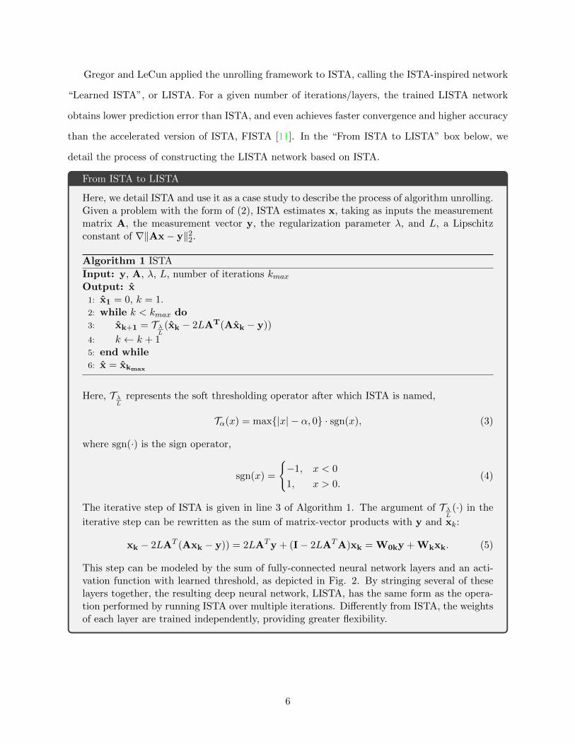
xk − 2LAT (Axk − y)) = 2LATy + (I− 2LATA)xk = W0ky + Wkxk. (5)

This step can be modeled by the sum of fully-connected neural network layers and an acti-vation function with learned threshold, as depicted in Fig. 2. By stringing several of theselayers together, the resulting deep neural network, LISTA, has the same form as the opera-tion performed by running ISTA over multiple iterations. Differently from ISTA, the weightsof each layer are trained independently, providing greater flexibility.

6

Figure 2: Unrolling of ISTA into LISTA. (a): Diagram of the operation of ISTA as a feedback loop.(b): Diagram of LISTA, matrix multiplications by 2LAT are replaced by the weight matrices, W0k, andmultiplication by I− 2LATA is replaced by Wk, which, along with W0k, may be optimized with supervisedlearning.

This framework provides several key advantages: first, algorithm parameters, such as λ in (2),

are learned automatically. Second, with an unrolled model, the part of the model corresponding to

A in (2), is learned, removing the need to explicitly model the PSF. Finally, while these iterative

algorithms are designed to solve a specific problem, sparse recovery, the approach is general, solving

all problems of this type equally well. With a neural network, the model can learn to analyze data

that may have additional structure not explainable by sparsity, and thereby obtain higher-accuracy

results more quickly. Because the underlying structure of the algorithm remains intact, the network

is also less prone to overfitting, improving robustness.

The unrolling framework also has a few drawbacks. The data-driven approach requires a sub-

stantial quantity of training data, which may be difficult to obtain. If the data used to train the

network is generated differently from that being analyzed (for example, if a different microscope

is used, with a substantially different PSF), recovery performance will degrade. However, it has

been found that learned unrolled networks are much more robust than traditional learned neural

networks to changes in the distribution of signal (for example, studying a different type of sub-

cellular structure [6]). The learned weights of the network may also be less interpretable than an

algorithm’s iterative step, in which each component has explicit physical meaning. In [6], however,

it is shown that the LISTA-based neural network used for the superresolution task learns transfor-

mations which are closely related to the operation of the iterative step (for instance, convolution

filters are learned with shapes similar to the PSF) and are easier to understand than those learned

by the purely data-driven approach of typical neural networks. It is also important to note that,

being partially data-driven, learned unrolled networks no longer explicitly solve the optimization

problems they are based on (such as sparse recovery). While the structure of the algorithm is

7

maintained, the transformation applied by the network does not follow the exact steps that are

guaranteed to find the minimizer of (2), and may not be applied in the image domain. So, while

learned unrolled networks have been shown to be successful in localizing spatially sparse sources,

they do not explicitly solve the sparse recovery problem.

Throughout the rest of the paper, we will concentrate on applications of deep unrolling to the

recovery of sparse biological data, specifically using unrolled networks based on ISTA. Importantly,

the learned unrolling strategy is not restricted to ISTA, nor is it restricted to problems with a

sparse prior: any algorithm for which the iterative step may be carried out by a learnable neural

network layer may be unrolled. Gregor and LeCun developed a learned version of the coordinate

descent algorithm, finding that the learned version again obtained much lower prediction error

than the iterative version[11]. Other authors have applied the unrolling framework to a variety of

algorithms for biological data processing tasks, including ADMM [18] and robust PCA [19], which

were shown to obtain lower errors in MRI signal recovery and ultrasound clutter suppression,

respectively, in less time than the then state-of-the-art algorithms, consistent with learned unrolled

networks converging more quickly. Outside of the realm of biology, in natural images unrolling of

the half-quadratic splitting algorithm has been shown to achieve both high-quality denoising [20]

and super-resolution in natural images[16]. Many additional example applications are provided in

a recent review [12].

4 Unrolling in Optical Localization Microscopy

In this section, we will focus on the domain of optical localization microscopy. First, we will give

a detailed example of how unrolling enhances the capabilities of one optical imaging technique:

Single-Molecule Localization Microscopy. Then, we will discuss how the concept of unrolling can

be applied to other sparse biological optical imaging problems.

4.1 Unrolling in Single-Molecule Localization Microscopy

Visualization of sub-cellular features and organelles within biological cells requires imaging tech-

niques with nanometer resolution. In the case of optical imaging systems, from the 19th century

until the recent development of super-resolution microscopy, the resolution limit was considered to

8

be set by Abbe’s diffraction limit for a microscope:

d =β

2NA, (6)

where d is the minimal distance below which two point sources cannot be distinguished, β is

the wavelength of the emitted photons, and NA is the numerical aperture of the microscope. In

fluorescence microscopy, the sample is stained with fluorophores which can be excited with one

color of light and emit photons of a higher wavelength for subsequent detection. Since most cells

are not naturally fluorescent, this allows specific imaging of the stained biomolecules. If the number

of photons emitted is sufficiently high, and the background is sufficiently low, single molecules can

be detected in this way. However, biological structures of interest are typically made of multitudes

of the same biomolecule type in close apposition, obscuring details finer than the diffraction limit

of the emitted photons when all fluorophores are emitting at the same time.

One may overcome the diffraction limit by distinguishing between the photons coming from

two neighboring fluorophores [21]. One way to distinguish neighboring molecules, is by utilizing

photo-activated or photo-switching fluorophores to separate fluorescent emission in time; this is

the basis for SMLM techniques such as Photo-Activated Localization Microscopy (PALM) and

Stochastic Optical Reconstruction Microscopy (STORM) [22, 23]. Optical, physical, or chemical

means are used to ensure that at any given moment only a small subset of all flurophores are emitting

photons. Then a large number of diffraction-limited images is collected, each containing just a few

active isolated fluorophores. The imaging sequence is long enough such that each fluorophore is

stochastically activated from a non-emissive state to a bright state, and back to a non-emissive

(or bleached) state. During each cycle, the density of activated molecules is kept low enough that

emission profiles of individual fluorophores do not overlap.

High-resolution fluorophore localization can be framed as a linear inverse problem. Let us

denote the collected sequence of diffraction-limited frames as Y ∈ RM2×T , where every column is

the M2 vector stacking of the corresponding M ×M frame. Our goal is to reconstruct an image

of size N × N , consisting of fluorophore locations on a fine grid (N > M). We can model the

generation of Y as:

9

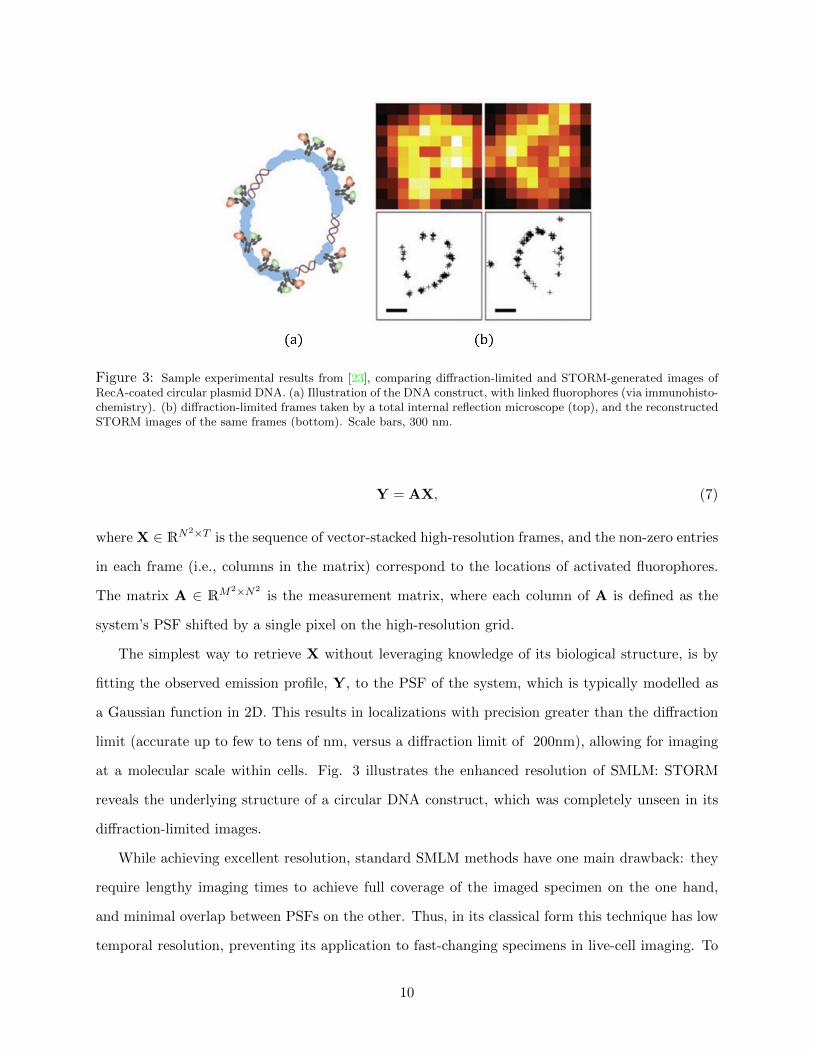
Figure 3: Sample experimental results from [23], comparing diffraction-limited and STORM-generated images ofRecA-coated circular plasmid DNA. (a) Illustration of the DNA construct, with linked fluorophores (via immunohisto-chemistry). (b) diffraction-limited frames taken by a total internal reflection microscope (top), and the reconstructedSTORM images of the same frames (bottom). Scale bars, 300 nm.

Y = AX, (7)

where X ∈ RN2×T is the sequence of vector-stacked high-resolution frames, and the non-zero entries

in each frame (i.e., columns in the matrix) correspond to the locations of activated fluorophores.

The matrix A ∈ RM2×N2is the measurement matrix, where each column of A is defined as the

system’s PSF shifted by a single pixel on the high-resolution grid.

The simplest way to retrieve X without leveraging knowledge of its biological structure, is by

fitting the observed emission profile, Y, to the PSF of the system, which is typically modelled as

a Gaussian function in 2D. This results in localizations with precision greater than the diffraction

limit (accurate up to few to tens of nm, versus a diffraction limit of 200nm), allowing for imaging

at a molecular scale within cells. Fig. 3 illustrates the enhanced resolution of SMLM: STORM

reveals the underlying structure of a circular DNA construct, which was completely unseen in its

diffraction-limited images.

While achieving excellent resolution, standard SMLM methods have one main drawback: they

require lengthy imaging times to achieve full coverage of the imaged specimen on the one hand,

and minimal overlap between PSFs on the other. Thus, in its classical form this technique has low

temporal resolution, preventing its application to fast-changing specimens in live-cell imaging. To

10

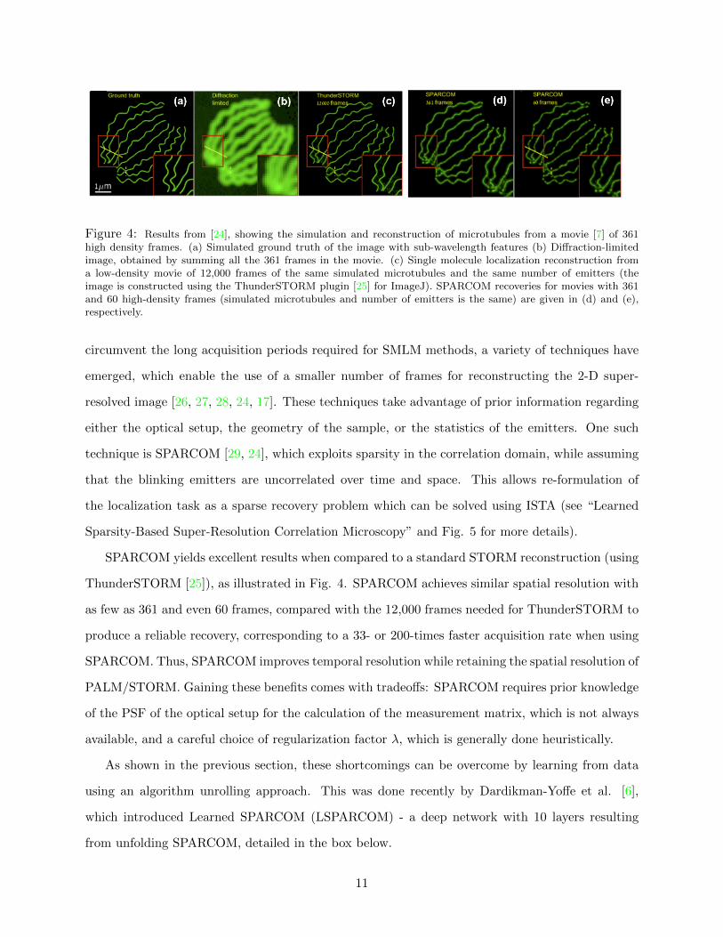
Figure 4: Results from [24], showing the simulation and reconstruction of microtubules from a movie [7] of 361high density frames. (a) Simulated ground truth of the image with sub-wavelength features (b) Diffraction-limitedimage, obtained by summing all the 361 frames in the movie. (c) Single molecule localization reconstruction froma low-density movie of 12,000 frames of the same simulated microtubules and the same number of emitters (theimage is constructed using the ThunderSTORM plugin [25] for ImageJ). SPARCOM recoveries for movies with 361and 60 high-density frames (simulated microtubules and number of emitters is the same) are given in (d) and (e),respectively.

circumvent the long acquisition periods required for SMLM methods, a variety of techniques have

emerged, which enable the use of a smaller number of frames for reconstructing the 2-D super-

resolved image [26, 27, 28, 24, 17]. These techniques take advantage of prior information regarding

either the optical setup, the geometry of the sample, or the statistics of the emitters. One such

technique is SPARCOM [29, 24], which exploits sparsity in the correlation domain, while assuming

that the blinking emitters are uncorrelated over time and space. This allows re-formulation of

the localization task as a sparse recovery problem which can be solved using ISTA (see “Learned

Sparsity-Based Super-Resolution Correlation Microscopy” and Fig. 5 for more details).

SPARCOM yields excellent results when compared to a standard STORM reconstruction (using

ThunderSTORM [25]), as illustrated in Fig. 4. SPARCOM achieves similar spatial resolution with

as few as 361 and even 60 frames, compared with the 12,000 frames needed for ThunderSTORM to

produce a reliable recovery, corresponding to a 33- or 200-times faster acquisition rate when using

SPARCOM. Thus, SPARCOM improves temporal resolution while retaining the spatial resolution of

PALM/STORM. Gaining these benefits comes with tradeoffs: SPARCOM requires prior knowledge

of the PSF of the optical setup for the calculation of the measurement matrix, which is not always

available, and a careful choice of regularization factor λ, which is generally done heuristically.

As shown in the previous section, these shortcomings can be overcome by learning from data

using an algorithm unrolling approach. This was done recently by Dardikman-Yoffe et al. [6],

which introduced Learned SPARCOM (LSPARCOM) - a deep network with 10 layers resulting

from unfolding SPARCOM, detailed in the box below.

11

Learned Sparsity-Based Super-Resolution Correlation Microscopy

In SPARCOM, we start by observing the temporal covariance matrices of X and Y, MX

and MY . According to (7), we can write the following:

MY = AMXAT . (8)

We assume that different emitters are uncorrelated over time and space. Thus, MX is adiagonal matrix, where each entry on its diagonal, m, represents the variance of the emitterfluctuation on a high-resolution grid. Since non-zero variance can only exist where there isfluctuation in emission, the support of the diagonal corresponds to the emitters’ locationson the high resolution grid. Therefore, recovering m and reshaping it as a matrix yields thedesired high-resolution image. For this purpose, let us re-write (8) as:

MY =

N2∑i=1

AiATi mi, (9)

where Ai is the i-th column in A and mi is the i-th entry in m. Following (2), we can exploitthe sparsity of emitters, and compute m by solving the following sparse recovery problem:

minm≥0

λ‖m‖1 +1

2‖MY −

N2∑i=1

AiATi mi‖22, (10)

where λ ≥ 0 is the regularization parameter. ISTA can be used to solve this optimizationproblem, as shown in 5.To apply unrolling to SPARCOM, we need to replace the operations performed in a singleiteration with neural network layers, and choose the input of the unrolled algorithm. Theunrolling process is illustrated in Fig. 5: to start, G, the N × N matrix-shaped resizedversion of the diagonal of MY , is taken as input. The matrix-multiplication operations

performed in each iteration are replaced with convolutional filters W(k)p , k=0, ..., 9, and the

positive soft-thresholding operator is replaced with a differentiable, sigmoid-based approxi-mation of the positive hard-thresholding operator [30], denoted as S+

α0,β0(·). The unrolling

process results in LSPARCOM - a deep neural network which acts as the operation doneby running SPARCOM over multiple iterations. LSPARCOM can be trained on a singlesequence of frames taken from one FOV with a known underlying structure, which can begenerated using simulations (like the one offered by ThunderSTORM [25]). The model isthen trained on overlapping small patches taken from multiple frames of that sequence.

12

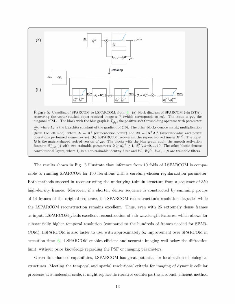
Figure 5: Unrolling of SPARCOM to LSPARCOM, from [6]. (a) block diagram of SPARCOM (via ISTA),recovering the vector-stacked super-resolved image x(k) (which corresponds to m). The input is gY , thediagonal of MY . The block with the blue graph is T λ

Lf

, the positive soft thresholding operator with parameter

λLf

, where Lf is the Lipschitz constant of the gradient of (10). The other blocks denote matrix multiplication

(from the left side), where A = A2 (element-wise power) and M = |ATA|2 (absolute-value and poweroperations performed element-wise). (b) LSPARCOM, recovering the super-resolved image X(k). The inputG is the matrix-shaped resized version of gY . The blocks with the blue graph apply the smooth activationfunction S+

α0,β0(·) with two trainable parameters: 0 ≥ α

(k)0 ≥ 1, β

(k)0 , k=0, ..., 10. The other blocks denote

convolutional layers, where If is a non-trainable identity filter and Wi, W(k)p , k=0, ..., 9 are trainable filters.

The results shown in Fig. 6 illustrate that inference from 10 folds of LSPARCOM is compa-

rable to running SPARCOM for 100 iterations with a carefully-chosen regularization parameter.

Both methods succeed in reconstructing the underlying tubulin structure from a sequence of 350

high-density frames. Moreover, if a shorter, denser sequence is constructed by summing groups

of 14 frames of the original sequence, the SPARCOM reconstruction’s resolution degrades while

the LSPARCOM reconstruction remains excellent. Thus, even with 25 extremely dense frames

as input, LSPARCOM yields excellent reconstruction of sub-wavelength features, which allows for

substantially higher temporal resolution (compared to the hundreds of frames needed for SPAR-

COM). LSPARCOM is also faster to use, with approximately 5x improvement over SPARCOM in

execution time [6]. LSPARCOM enables efficient and accurate imaging well below the diffraction

limit, without prior knowledge regarding the PSF or imaging parameters.

Given its enhanced capabilities, LSPARCOM has great potential for localization of biological

structures. Meeting the temporal and spatial resolutions’ criteria for imaging of dynamic cellular

processes at a molecular scale, it might replace its iterative counterpart as a robust, efficient method

13

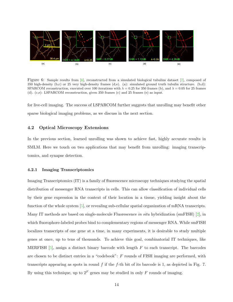
Figure 6: Sample results from [6], reconstructed from a simulated biological tubulins dataset [7], composed of350 high-density (b,c) or 25 very high-density frames (d,e). (a): simulated ground truth tubulin structure. (b,d):SPARCOM reconstruction, executed over 100 iterations with λ = 0.25 for 350 frames (b), and λ = 0.05 for 25 frames(d). (c,e): LSPARCOM reconstruction, given 350 frames (c) and 25 frames (e) as input.

for live-cell imaging. The success of LSPARCOM further suggests that unrolling may benefit other

sparse biological imaging problems, as we discuss in the next section.

4.2 Optical Microscopy Extensions

In the previous section, learned unrolling was shown to achieve fast, highly accurate results in

SMLM. Here we touch on two applications that may benefit from unrolling: imaging transcrip-

tomics, and synapse detection.

4.2.1 Imaging Transcriptomics

Imaging Transcriptomics (IT) is a family of fluorescence microscopy techniques studying the spatial

distribution of messenger RNA transcripts in cells. This can allow classification of individual cells

by their gene expression in the context of their location in a tissue, yielding insight about the

function of the whole system [5], or revealing sub-cellular spatial organization of mRNA transcripts.

Many IT methods are based on single-molecule Fluorescence in situ hybridization (smFISH) [2], in

which fluorophore-labeled probes bind to complementary regions of messenger RNA. While smFISH

localizes transcripts of one gene at a time, in many experiments, it is desirable to study multiple

genes at once, up to tens of thousands. To achieve this goal, combinatorial IT techniques, like

MERFISH [5], assign a distinct binary barcode with length F to each transcript. The barcodes

are chosen to be distinct entries in a “codebook”: F rounds of FISH imaging are performed, with

transcripts appearing as spots in round f if the f -th bit of its barcode is 1, as depicted in Fig. 7.

By using this technique, up to 2F genes may be studied in only F rounds of imaging.

14

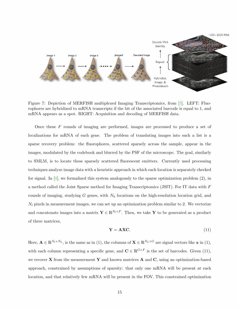
Figure 7: Depiction of MERFISH multiplexed Imaging Transcriptomics, from [5]. LEFT: Fluo-rophores are hybridized to mRNA transcripts if the bit of the associated barcode is equal to 1, andmRNA appears as a spot. RIGHT: Acquisition and decoding of MERFISH data.

Once these F rounds of imaging are performed, images are processed to produce a set of

localizations for mRNA of each gene. The problem of translating images into such a list is a

sparse recovery problem: the fluorophores, scattered sparsely across the sample, appear in the

images, modulated by the codebook and blurred by the PSF of the microscope. The goal, similarly

to SMLM, is to locate these sparsely scattered fluorescent emitters. Currently used processing

techniques analyze image data with a heuristic approach in which each location is separately checked

for signal. In [8], we formalized this system analogously to the sparse optimization problem (2), in

a method called the Joint Sparse method for Imaging Transcriptomics (JSIT). For IT data with F

rounds of imaging, studying G genes, with Nh locations on the high-resolution location grid, and

Nl pixels in measurement images, we can set up an optimization problem similar to 2. We vectorize

and concatenate images into a matrix Y ∈ RNl×F . Then, we take Y to be generated as a product

of three matrices,

Y = AXC. (11)

Here, A ∈ RNl×Nh , is the same as in (1), the columns of X ∈ RNh×G are signal vectors like x in (1),

with each column representing a specific gene, and C ∈ RG×F is the set of barcodes. Given (11),

we recover X from the measurement Y and known matrices A and C, using an optimization-based

approach, constrained by assumptions of sparsity: that only one mRNA will be present at each

location, and that relatively few mRNA will be present in the FOV. This constrained optimization

15

problem can be solved with an iterative algorithm. In addition to being more interpretable than

the currently used heuristic, this method has achieved more accurate mRNA localization, especially

in low-magnification imaging.

A natural extension of this formulation is the application of learned unrolling. Based on our

experience with other applications, unrolling may improve performance obtaining more accurate

genetic expression levels in fewer iterations, while eliminating parameter-tuning requirements and

explicit knowledge of the optical PSF A.

4.2.2 Synapse Detection

Many other biological settings involve sparse emitters, but have not necessarily been framed as

sparse recovery problems to improve performance. For example, sparse biological images are en-

countered in neuronal synapse detection for characterization of the neurophysiological consequences

of genetic and pharmacological perturbation screens. Synapses are localized by identifying positions

in which fluorescently tagged pre- and post-synaptic proteins are located in close proximity. These

proteins cluster into puncta which appear as point sources, similar to fluorophores in SMLM data.

Sparse analysis could identify sub-pixel locations for each punctum, and, from the presence of both

pre- and post-synaptic proteins, infer accurate synapse locations. While sparse algorithm unrolling

has not yet been applied in this context, model-based learning strategies have already shown good

results [3] for this setting.

5 Unrolling in other imaging modalities

Sparse emitters arise in other biological imaging modalities beyond epifluorescent microscopy, and

the algorithmic unrolling method has achieved fast, highly accurate localization in several such

settings. Here we will review three such cases: Ultrasound Localization Microscopy (ULM), Light

Field Microscopy (LFM), and cell center localization in non-spatially-sparse histology images.

5.1 Unrolling in Ultrasound Localization Microscopy

The attainable resolution of ultrasonography is fundamentally limited by wave diffraction, i.e., the

minimum distance between separable scatters is half a wavelength. Due to this limit, conventional

16

ultrasound techniques are bound to a tradeoff between resolution and penetration depth: increases

in the transmit frequency shortens the wavelength (thus increasing resolution) but come at the cost

of reduced penetration depth, since higher frequency waves suffer from stronger absorption. This

tradeoff particularly hinders deep high-resolution microvascular imaging, which is crucial for many

diagnostic applications.

A decade ago, this tradeoff was circumvented by the introduction of Ultrasound Localization

Microscopy (ULM) [9, 31], which leverages the principles of SMLM and adapts these to ultrasound

imaging. In SMLM, stochastic “blinking” of subsets of fluorophores is exploited to provide sparse

point sources; in ULM, lipid-shelled gas microbubbles fulfill this role. A sequence of diffraction-

limited ultrasonic scans is acquired, each containing just a few active isolated sources. Thus, each

received image frame can be written as:

y = Ax + w, (12)

where x is a vector that describes the sparse microbubble distribution on a high-resolution image

grid, y is a vectorized image frame from the ultrasound sequence, A is the measurement matrix

(defined by the system’s PSF), and w is a noise vector. As in SMLM, this enables precise localization

of their centers on a subdiffraction grid. The accumulation of many such localizations over time

yields a super-resolved image. This approach achieves a resolution up to ten times smaller than

the wavelength [32], showing that ultrasonography at sub-diffraction scale is possible.

Similarly to SMLM, the quality of ULM imaging is dependant on the quantity of localized

microbubbles and localization accuracy; thus, it gives rise to a new tradeoff between microbubble

density and acquisition time. To achieve the desired signal sparsity for straightforward isolation of

the backscattered echoes, ULM is typically performed using a very diluted solution of microbubbles.

On regular ultrasound systems, this constraint leads to tediously long acquisition times to cover

the full vascular bed. Ultrafast plane-wave ultrasound (uULM) imaging has managed to lower ac-

quisition time [32] by taking many snapshots of individual microbubbles, as they transport through

the vasculature, thereby facilitating high-fidelity reconstruction of the larger vessels. Nevertheless,

mapping the full capillary bed still requires microbubbles to pass through each capillary, capping

acquisition time benefits to tens of minutes [33].

17

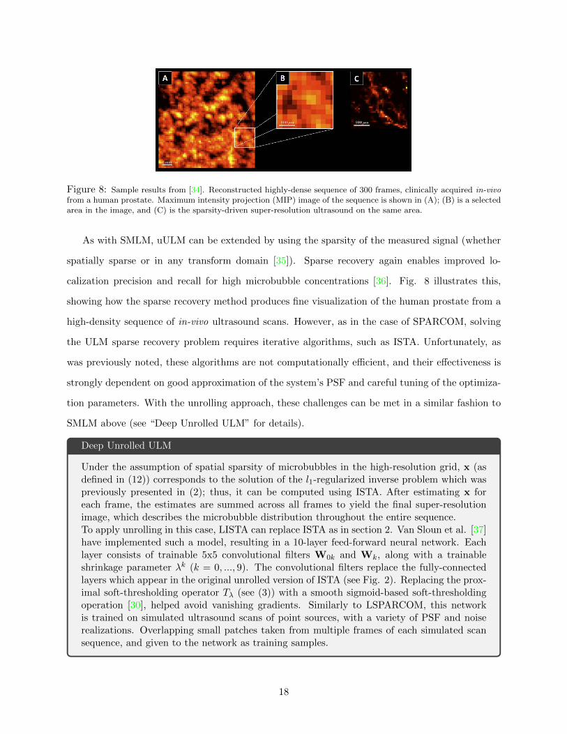
Figure 8: Sample results from [34]. Reconstructed highly-dense sequence of 300 frames, clinically acquired in-vivofrom a human prostate. Maximum intensity projection (MIP) image of the sequence is shown in (A); (B) is a selectedarea in the image, and (C) is the sparsity-driven super-resolution ultrasound on the same area.

As with SMLM, uULM can be extended by using the sparsity of the measured signal (whether

spatially sparse or in any transform domain [35]). Sparse recovery again enables improved lo-

calization precision and recall for high microbubble concentrations [36]. Fig. 8 illustrates this,

showing how the sparse recovery method produces fine visualization of the human prostate from a

high-density sequence of in-vivo ultrasound scans. However, as in the case of SPARCOM, solving

the ULM sparse recovery problem requires iterative algorithms, such as ISTA. Unfortunately, as

was previously noted, these algorithms are not computationally efficient, and their effectiveness is

strongly dependent on good approximation of the system’s PSF and careful tuning of the optimiza-

tion parameters. With the unrolling approach, these challenges can be met in a similar fashion to

SMLM above (see “Deep Unrolled ULM” for details).

Deep Unrolled ULM

Under the assumption of spatial sparsity of microbubbles in the high-resolution grid, x (asdefined in (12)) corresponds to the solution of the l1-regularized inverse problem which waspreviously presented in (2); thus, it can be computed using ISTA. After estimating x foreach frame, the estimates are summed across all frames to yield the final super-resolutionimage, which describes the microbubble distribution throughout the entire sequence.To apply unrolling in this case, LISTA can replace ISTA as in section 2. Van Sloun et al. [37]have implemented such a model, resulting in a 10-layer feed-forward neural network. Eachlayer consists of trainable 5x5 convolutional filters W0k and Wk, along with a trainableshrinkage parameter λk (k = 0, ..., 9). The convolutional filters replace the fully-connectedlayers which appear in the original unrolled version of ISTA (see Fig. 2). Replacing the prox-imal soft-thresholding operator Tλ (see (3)) with a smooth sigmoid-based soft-thresholdingoperation [30], helped avoid vanishing gradients. Similarly to LSPARCOM, this networkis trained on simulated ultrasound scans of point sources, with a variety of PSF and noiserealizations. Overlapping small patches taken from multiple frames of each simulated scansequence, and given to the network as training samples.

18

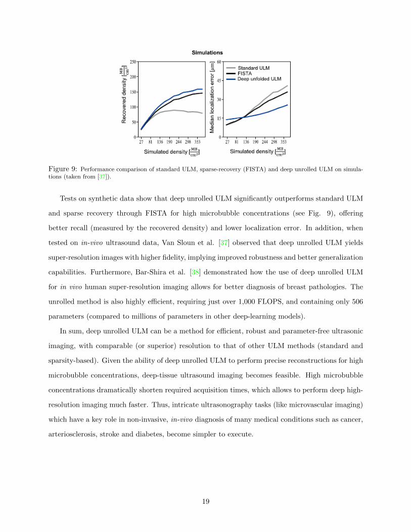
Figure 9: Performance comparison of standard ULM, sparse-recovery (FISTA) and deep unrolled ULM on simula-tions (taken from [37]).

Tests on synthetic data show that deep unrolled ULM significantly outperforms standard ULM

and sparse recovery through FISTA for high microbubble concentrations (see Fig. 9), offering

better recall (measured by the recovered density) and lower localization error. In addition, when

tested on in-vivo ultrasound data, Van Sloun et al. [37] observed that deep unrolled ULM yields

super-resolution images with higher fidelity, implying improved robustness and better generalization

capabilities. Furthermore, Bar-Shira et al. [38] demonstrated how the use of deep unrolled ULM

for in vivo human super-resolution imaging allows for better diagnosis of breast pathologies. The

unrolled method is also highly efficient, requiring just over 1,000 FLOPS, and containing only 506

parameters (compared to millions of parameters in other deep-learning models).

In sum, deep unrolled ULM can be a method for efficient, robust and parameter-free ultrasonic

imaging, with comparable (or superior) resolution to that of other ULM methods (standard and

sparsity-based). Given the ability of deep unrolled ULM to perform precise reconstructions for high

microbubble concentrations, deep-tissue ultrasound imaging becomes feasible. High microbubble

concentrations dramatically shorten required acquisition times, which allows to perform deep high-

resolution imaging much faster. Thus, intricate ultrasonography tasks (like microvascular imaging)

which have a key role in non-invasive, in-vivo diagnosis of many medical conditions such as cancer,

arteriosclerosis, stroke and diabetes, become simpler to execute.

19

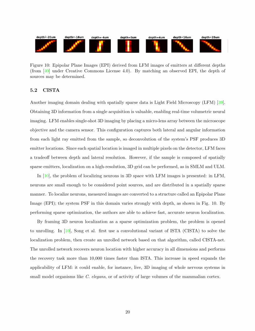
Figure 10: Epipolar Plane Images (EPI) derived from LFM images of emitters at different depths(from [40] under Creative Commons License 4.0). By matching an observed EPI, the depth ofsources may be determined.

5.2 CISTA

Another imaging domain dealing with spatially sparse data is Light Field Microscopy (LFM) [39].

Obtaining 3D information from a single acquisition is valuable, enabling real-time volumetric neural

imaging. LFM enables single-shot 3D imaging by placing a micro-lens array between the microscope

objective and the camera sensor. This configuration captures both lateral and angular information

from each light ray emitted from the sample, so deconvolution of the system’s PSF produces 3D

emitter locations. Since each spatial location is imaged in multiple pixels on the detector, LFM faces

a tradeoff between depth and lateral resolution. However, if the sample is composed of spatially

sparse emitters, localization on a high-resolution, 3D grid can be performed, as in SMLM and ULM.

In [10], the problem of localizing neurons in 3D space with LFM images is presented: in LFM,

neurons are small enough to be considered point sources, and are distributed in a spatially sparse

manner. To localize neurons, measured images are converted to a structure called an Epipolar Plane

Image (EPI); the system PSF in this domain varies strongly with depth, as shown in Fig. 10. By

performing sparse optimization, the authors are able to achieve fast, accurate neuron localization.

By framing 3D neuron localization as a sparse optimization problem, the problem is opened

to unrolling. In [10], Song et al. first use a convolutional variant of ISTA (CISTA) to solve the

localization problem, then create an unrolled network based on that algorithm, called CISTA-net.

The unrolled network recovers neuron location with higher accuracy in all dimensions and performs

the recovery task more than 10,000 times faster than ISTA. This increase in speed expands the

applicability of LFM: it could enable, for instance, live, 3D imaging of whole nervous systems in

small model organisms like C. elegans, or of activity of large volumes of the mammalian cortex.

20

5.3 Non-Spatially Sparse Imaging

The most obvious way of thinking about sparse recovery in biological imaging is in the domain of

spatially sparse sources, but there are other methods which leverage sparse coding in other aspects,

and unrolling can achieve accurate results in these situations as well.

One example is cell center localization in histology slides. While cell centers are scattered

sparsely in a FOV, cell shapes are irregular, so there is not a single “impulse response” transforming

cell center locations into images of cells, as in the sparse recovery form of (2). In [4], a traditional

CNN is combined with a LISTA-like network to localize cell centers. In this framework, the locations

of the centers of cells in a 2-dimensional FOV with dimension h × w are represented by a binary

matrix X ∈ Rh×w. The matrix X is Radon transformed to represent the cell centers in polar

coordinates, Xp = Rf(X). A measurement matrix A is generated as a random Gaussian projection

matrix, and the product AXp = Y is formed. Xue et al. found that although Y cannot be measured

directly, a CNN may be trained to infer Y from an image of the FOV. A two-stage neural network

is designed: the first stage a traditional CNN, transforming the images into an estimate Y of the

matrix Y, the second stage a LISTA-like network used to obtain an estimate Xp of the sparse

matrix Xp, which, after inverse Radon transformation, gives the cell center locations X. The

network, called End-to-end Convolutional Neural Network and Compressed Sensing (ECNNCS),

is trained by penalizing the differences between both y and y and x and x. The ECNNCS model

achieved better localization accuracy than the state-of-the-art algorithms used as comparison [4],

showing that unrolling can improve performance outside problems of strict spatial sparsity.

Another technique in which sparse recovery may be applied to biological imaging data which

is not spatially sparse is Compressed in situ Imaging (CISI) [41], and we propose that algorithm

unrolling will improve performance in this method as well. Like Imaging Transcriptomics (IT),

CISI is a microscopy technique which evaluates expression levels of genes at single-cell resolution.

Different from IT, in CISI data are not spatially sparse. Instead, CISI takes advantage of genetic co-

expression patterns to infer single cells’ transcriptomes from a few measurements of multiple genes at

once (“composite measurements”). In CISI, single-cell transcriptomes are conceptualized as linear

combinations of “modules”, (sparse) linear combinations of co-expressed genes. The sparse recovery

problem is to infer from composite measurements of genes the sparse set of active co-expression

21

modules. Currently, modules are defined before the experiment, but with algorithmic unrolling,

optimal co-expression modules could be learned, enabling improved transcriptome inference.

6 Conclusion

New biological imaging techniques are constantly being developed, and with them, computational

pipelines to identify and characterize the imaged biological structures. We have described a few

of these techniques and their accompanying pipelines. In many cases, these techniques consist of

heuristic strategies which have limited accuracy and are difficult to interpret. As computational

power continues to increase and the methods become more developed, more powerful, interpretable

processing techniques have been created by incorporating biological and physical assumptions into

constrained optimization problems, solved with iterative methods. These in turn require parameter

tuning and explicit knowledge of the experimental setup. A natural next step in pipeline develop-

ment is model-based learning methods, including algorithmic unrolling. We have shown how, in

many imaging modalities requiring source localization, unrolling achieves fast, accurate results with

robust models, and proposed that unrolling be extended widely to other similar problems, includ-

ing to methods involving biological structure other than sparsity. We hope this work will inspire

methods extending unrolling to further biological imaging modalities and experimental settings.

References

[1] X. Zhuang, “Nano-imaging with STORM,” Nature photonics, vol. 3, no. 7, pp. 365–367, 2009.

[2] A.M. Femino, F.S. Fay, K. Fogarty, and R.H. Singer, “Visualization of single RNA transcriptsin situ,” Science, vol. 280, pp. 585–590, 1998.

[3] V. Kulikov, S.-M. Guo, M. Stone, A. Goodman, A. Carpenter, M. Bathe, and V. Lempitsky,“Dognet: A deep architecture for synapse detection in multiplexed fluorescence images,” PLOSComputational Biology, vol. 15, 2019.

[4] Y. Xue, G. Bigras, J. Hugh, and N. Ray, “Training convolutional neural networks and com-pressed sensing end-to-end for microscopy cell detection,” IEEE transactions on medical imag-ing, vol. 38, no. 11, pp. 2632–2641, 2019.

[5] K.H. Chen, A.N. Boettiger, J.R. Moffitt, S. Wang, and X. Zhuang, “Spatially resolved, highlymultiplexed RNA profiling in single cells,” Science, vol. 348, pp. 412, 2015.

[6] G. Dardikman-Yoffe and Y. C. Eldar, “Learned SPARCOM: Unfolded deep super-resolutionmicroscopy,” Optics Express, vol. 28-19, pp. 27736 – 27763, September 2020.

[7] D. Sage, H. Kirshner, T. Pengo, N. Stuurman, J. Min, S. Manley, and M. Unser, “Quantitativeevaluation of software packages for single-molecule localization microscopy,” Nature methods,vol. 12, no. 8, pp. 717–724, 2015.

22

[8] J. Bryan, B. Cleary, S. Farhi, and Y.C. Eldar, “Sparse recovery of imaging transcriptomicsdata,” Proceedings of the International Symposium on Biomedical Imaging, 2021.

[9] I. Grundberg, S. Kiflemariam, M. Mignardi, K. Imgenberg, K. Edlund, P. Micke, M. Sund-strom, T. Sjoblom, J. Botling, and M. Nilsson, “Super-resolution ultrasound imaging,” Ultra-sound in medicine and biology, vol. 46, pp. 865–891, 2020.

[10] P. Song, H. V. Jadan, C. L. Howe, P. Quicke, A. J. Foust, and P. L. Dragotti, “Model-inspireddeep learning for light-field microscopy with application to neuron localization,” arXiv preprintarXiv:2103.06164, 2021.

[11] K. Gregor and Y. LeCun, “Learning fast approximations of sparse coding,” Proc. of 27th Int.Conf. on machine learning, pp. 399 – 406, 2010.

[12] V. Monga, Y. Li, and Y. C. Eldar, “Algorithm unrolling: Interpretable, efficient deep learningfor signal and image processing,” IEEE Signal Processing Magazine, pp. 17–43, 2021.

[13] R. Tibshirani, “Regression shrinkage and selection via the lasso,” Journal of the Royal Sta-tistical Society. Series B (Methodological), vol. 58-1, pp. 267 – 288, 1996.

[14] S. Boyd, N. Parikh, E. Chu, B. Peleato, and J. Eckstein, “Distributed optimization andstatistical learning via the alternating direction method of multipliers,” Foundations andTrends in Machine Learning, vol. 3, pp. 1–122, 2011.

[15] I. Daubechies, M. Defrise, and C.De Mol, “An iterative thresholding algorithm for linear inverseproblems with sparsity constraint,” Communications on on Pure and Applied Mathematics,vol. 57-11, pp. 1413–1457, November 2004.

[16] K. Zhang, L. V. Gool, and R. Timofte, “Deep unfolding network for image super-resolution,”in Proceedings of the IEEE/CVF Conference on Computer Vision and Pattern Recognition,2020, pp. 3217–3226.

[17] E. Nehme, L. E. Weiss, T. Michaeli, , and Y. Shechtman, “Deep-STORM: super-resolutionsingle-molecule microscopy by deep learning,” Optica, vol. 5, pp. 458–464, 2018.

[18] Y. Yang, J. Sun, H. Li, and Z. Xu, “Deep ADMM-Net for compressive sensing MRI,” inProceedings of the 30th International Conference on Neural Information Processing Systems,Red Hook, NY, USA, 2016, NIPS’16, p. 10–18, Curran Associates Inc.

[19] O. Solomon, R. Cohen, Y. Zhang, Y. Yang, Q. He, J. Luo, R. JG van Sloun, and Y. C. Eldar,“Deep unfolded robust PCA with application to clutter suppression in ultrasound,” IEEEtransactions on medical imaging, vol. 39, no. 4, pp. 1051–1063, 2019.

[20] Y. Li, M. Tofighi, J. Geng, V. Monga, and Y. C. Eldar, “Efficient and interpretable deep blindimage deblurring via algorithm unrolling,” IEEE Transactions on Computational Imaging,vol. 6, pp. 666–681, 2020.

[21] E. Betzig, “Proposed method for molecular optical imaging,” Optics Letters, vol. 20, pp.237–239, 1995.

[22] E. Betzig, G. H. Patterson, R. Sougratand O. W. Lindwasser, S. Olenych, J. S. Bonifacino,M. W. Davidson, J. Lippincott-Schwartz, and H. F. Hess, “Imaging intracellular fluorescentproteins at nanometer resolution,” Science, vol. 313, pp. 1642–1645, September 2006.

[23] M. J. Rust, M. Bates, and X. Zhuang, “Sub-diffraction-limit imaging by stochastic opticalreconstruction microscopy (STORM),” Nature Methods, vol. 3, pp. 793–796, August 2006.

[24] O. Solomon, M. Mutzafi, M. Segev, and Y. C. Eldar, “Sparsity-based super-resolution mi-croscopy from correlation information,” Optics Express, vol. 26-14, pp. 18238–18269, June2018.

23

[25] M. Ovesny, P. Krızek, J. Borkovec, Z. Svindrych, and G. M. Hagen, “ThunderSTORM:a comprehensive imagej plug-in for PALM and STORM data analysis and super-resolutionimaging,” Bioinformatics, vol. 30, no. 16, pp. 2389–2390, 2014.

[26] J. Min, C. Vonesch, H. Kirshner, L. Carlini, N. Olivier, S. Holden, S. Manley, J. C. Ye,and M. Unser, “FALCON: fast and unbiased reconstruction of high-density super-resolutionmicroscopy data,” Scientific Reports, vol. 4, pp. 1–9, 2014.

[27] L. Zhu, W. Zhang, D. Elnatan, and B. Huang, “Faster STORM using compressed sensing,”Nature Methods, vol. 9, pp. 721–726, 2012.

[28] T. Dertinger, R. Colyer, G. Iyer, S. Weiss, and J. Enderlein, “Fast, background-free, 3Dsuper-resolution optical fluctuation imaging (SOFI),” Proceedings of the National Academy ofSciences of the United States of America, vol. 106(52), pp. 22287–22292, 2009.

[29] O. Solomon, Y. C. Eldar, M. Mutzafi, and M. Segev, “SPARCOM: Sparsity based super-resolution correlation microscopy,” SIAM J. on Img. Sci., vol. 12-1, pp. 392–419, Feb. 2019.

[30] X.P. Zhang, “Thresholding neural network for adaptive noise reduction,” IEEE transactionson neural networks, vol. 10, pp. 567–584, 2001.

[31] Y. Desailly, O. Couture, M. Fink, and M. Tanter, “Sono-activated ultrasound localizationmicroscopy,” Applied Physics Letters, vol. 103, pp. 174107, 2013.

[32] C. Errico, J. Pierre, S. Pezet, Y. Desailly, Z. Lenkei, O. Couture, and M. Tanter, “Ultrafastultrasound localization microscopy for deep super-resolution vascular imaging,” Nature, vol.527, pp. 499–502, 2015.

[33] V. Hingot, C. Errico, B. Heiles, L. Rahal, M. Tanter, and O. Couture, “Microvascular flow dic-tates the compromise between spatial resolution and acquisition time in ultrasound localizationmicroscopy,” Scientific Reports, vol. 9, 2019.

[34] O. Solomon, R. van Sloun, H. Wijkstra, M. Mischi, and Y. C. Eldar, “Sparsity-driven super-resolution in clinical contrast-enhanced ultrasound,” IEEE International Ultrasonics Sympo-sium, pp. 1–4, 2017.

[35] A. Bar-Zion, O. Solomon, C. Tremblay-Darveau, D. Adam, and Y. C. Eldar, “SUSHI: Sparsity-based ultrasound super-resolution hemodynamic imaging,” IEEE Transactions on Ultrasonics,Ferroelectrics, and Frequency Control, vol. 65, pp. 2365–2380, 2018.

[36] O. Solomon, R. van Sloun, H. Wijkstra, M. Mischi, and Y. C. Eldar, “Exploiting flow dynam-ics for superresolution in contrast-enhanced ultrasound,” IEEE Transactions on Ultrasonics,Ferroelectrics, and Frequency Control, vol. 66, pp. 1573–1586, 2019.

[37] R. van Sloun, R. Cohen, and Y. C. Eldar, “Deep learning in ultrasound imaging,” Proceedingsof the IEEE, vol. 108, pp. 11–29, 2020.

[38] O. Bar-Shira, A. Grubstein, Y. Rapson, D. Suhami, E. Atar, K. Peri-Hanania, R. Rosen, andY. C. Eldar, “Learned super resolution ultrasound for improved breast lesion characterization,”International Conference on Medical Image Computing and Computer Assisted Intervention,pp. 1–10, 2021.

[39] M. Levoy, R. Ng, A. Adams, M. Footer, and M. Horowitz, “Light field microscopy,” in ACMSIGGRAPH 2006 Papers, pp. 924–934. 2006.

[40] P. Song, H. V. Jadan, C. L. Howe, P. Quicke, A. J. Foust, and P. L. Dragotti, “3D local-ization for light-field microscopy via convolutional sparse coding on epipolar images,” IEEETransactions on Computational Imaging, vol. 6, pp. 1017–1032, 2020.

[41] B. Cleary, B. Simonton, J. Bezney, E. Murray, S. Alam, A. Sinha, E. Habibi, J. Marshall, E. S.Lander, F. Chen, and A. Regev, “Compressed sensing for imaging transcriptomics,” bioRxiv,2020.

24