Embed Size (px)
Citation preview
Sparse Autoencoder-Based Multi-Head Deep NeuralNetworks for Machinery Fault Diagnostics WithNovelty DetectionZhe Yang
Dongguan University of TechnologyDejan Gjorgjevikj
SS Cyril and Methodius UniversityJian-Yu Long
Dongguan University of TechnologyYan-Yang Zi
Xi'an Jiaotong UniversityShao-Hui Zhang
Dongguan University of TechnologyChuan Li ( [email protected] )
Dongguan University of Technology https://orcid.org/0000-0001-8437-6408
Original Article
Keywords: Deep learning, Fault diagnostics, Novelty detection, Multi-head deep neural network, Sparseautoencoder
Posted Date: December 10th, 2020
DOI: https://doi.org/10.21203/rs.3.rs-122416/v1
License: This work is licensed under a Creative Commons Attribution 4.0 International License. Read Full License
·1·
Title page
Sparse Autoencoder-based Multi-head Deep Neural Networks for Machinery Fault
Diagnostics with Novelty Detection
Zhe Yang1,3
E-mail: [email protected]
Dejan Gjorgjevikj2
Email: [email protected]
Jian-Yu Long1
E-mail: [email protected]
Yan-Yang Zi3
E-mail: [email protected]
Shao-Hui Zhang1
E-mail: [email protected]
Chuan Li1
E-mail: [email protected]
1 School of Mechanical Engineering, Dongguan University of Technology, Dongguan, 523808, China 2 Faculty of Computer Science and Engineering, Ss. Cyril and Methodius University, Skopje, North Macedonia 3 School of Mechanical Engineering, Xi’an Jiaotong University, Xi’an, 710049, China
Corresponding author: Chuan Li E-mail: [email protected]
Zhe Yang et al.
·2·
ORIGINAL ARTICLE
Sparse Autoencoder-based Multi-head Deep Neural Networks for Machinery
Fault Diagnostics with Novelty Detection Zhe Yang1,3, Dejan Gjorgjevikj2, Jian-Yu Long1, Yan-Yang Zi3, Shao-Hui Zhang1, Chuan Li1*
Received December xx, 2020; revised February xx, 2021; accepted March xx, 2021
Abstract: Novelty detection is a challenging task for the
machinery fault diagnosis. A novel fault diagnostic method is
developed for dealing with not only diagnosing the known type of
defect, but also detecting novelties, i.e. the occurrence of new
types of defects which have never been recorded. To this end, a
sparse autoencoder-based multi-head Deep Neural Network (DNN)
is presented to jointly learn a shared encoding representation for
both unsupervised reconstruction and supervised classification of
the monitoring data. The detection of novelties is based on the
reconstruction error. Moreover, the computational burden is
reduced by directly training the multi-head DNN with rectified
linear unit activation function, instead of performing the
pre-training and fine-tuning phases required for classical DNNs.
The addressed method is applied to a benchmark bearing case
study and to experimental data acquired from a delta 3D printer.
The results show that it is able to accurately diagnose known
types of defects, as well as to detect unknown defects,
outperforming other state-of-the-art methods.
Keywords: Deep learning • Fault diagnostics • Novelty detection
• Multi-head deep neural network • Sparse autoencoder
1 Introduction
With the objective of increasing the availability and
reducing operation and maintenance cost of mechanical
systems, Prognostics and Health Management (PHM) Chuan Li
1 School of Mechanical Engineering, Dongguan University of
Technology, Dongguan, 523808, China
2 Faculty of Computer Science and Engineering, Ss. Cyril and
Methodius University, Skopje, North Macedonia
3 School of Mechanical Engineering, Xi’an Jiaotong University, Xi’an,
710049, China
approaches has been getting more and more attention [1–3].
Fault diagnostics is one of the fundamental tasks of PHM,
which aims at detecting and diagnosing machinery failure
using model-based or data-driven approaches [4]. In the era
of Industry 4.0, since mechanical systems are getting more
and more complex, it is very difficult and expensive to
develop physics-based degradation models required for
model-based approaches. Whereas the increased
availability of data collected from multiple monitoring
sensors and the grown ability of processing data by
artificial intelligence algorithms have brought the great
potential for the development of advanced data-driven
approaches [5]. Data-driven approaches are typically based
on the development of an empirical classification model
trained on monitoring data. Chine et al. [6] proposed a fault
diagnostics approach for the photovoltaic system based on
Artificial Neural Networks (ANNs). Malik et al. [7] used
Empirical Mode Decomposition (EMD) for feature
extraction, and an ANN was trained using the extracted
features for gearbox fault diagnostics. He et al. [8]
extracted statistical features from monitoring signals and
Support Vector Machines (SVMs) were developed for fault
diagnostics for the 3D printer. Li et al. [9] utilized wavelet
packet decomposition and SVM for the diagnostics of
machinery faults of high-voltage circuit breaker failures.
Liu et al. [10] proposed a bearing diagnostics approach
which combined EMD and auto-regressive model to extract
features from vibration signals and used random forests to
set an effective classification model. Hu et al. [11]
developed a wind turbine bearing fault diagnosis based on
multi-masking EMD and fuzzy c-means clustering. Other
approaches, such as k-nearest neighbor [12], naïve Bayes
[13], linear discriminant analysis [14], fuzzy petri nets [15],
extreme learning machines [16], have also been
Sparse Autoencoder-based Multi-head Deep Neural Networks for Machinery Fault Diagnostics with Novelty Detection
·3·
successfully developed for fault diagnostics.
Although these intelligent fault diagnostics approaches
have shown great progress, there are still some limitations.
On the one hand, they rely on the identification of
handcrafted features requiring expert knowledge or
computationally demanding feature selection methods. On
the other hand, the shallow learning architecture of these
approaches leads to poor performance for complex
classification problems. To address these difficulties,
recently Deep Learning (DL) methods have been
extensively applied for machinery fault diagnostics[17–20].
DL methods are expected to automatically provide
high-level representation by using neural networks with
multiple layers of non-linear transformations, without
requiring human-designed and labor-intensive analyses of
the data [21,22]. Jia et al. [23] fed the frequency spectra of
vibration signals into stacked AutoEncoders (AEs)-based
Deep Neural Networks (DNNs) for rotating machinery
diagnostics. Chen et al. [24] proposed Sparse AutoEncoder
(SAE) and deep belief network for fault diagnosis of
bearings. Lu et al. [25] employed denoising AEs for fault
diagnostics of rotating machinery components. Shao et al.
[26] presented a deep belief network by stacking multiple
restricted Boltzmann machines for fault diagnostics of
induction motors. Wang et al. [27] employed Convolutional
Neural Networks (CNNs) for fault diagnostics of motors,
where the input is the time-frequency map of the vibration
signal. Jiang et al. [28] presented a method incorporating
multiscale learning into the traditional CNN architecture
for defect identification of wind turbine gearbox. Chang et
al. [29] proposed a concurrent CNN composed of parallel
convolution layers with multi-scale kernels for fault
diagnosis of wind turbine bearings. Yuan et al. [30]
investigated the development of different Recurrent Neural
Networks (RNNs) including vanilla RNN, Long
Short-Term Memory (LSTM) and gated recurrent unit for
fault diagnostics and prognostics of aero engine. Chen et al.
[31] utilized multi-scale CNNs to extract features that are
then fed to a LSTM for bearing fault diagnostics. Echo
State Networks (ESNs), another type of RNN characterized
by high training efficiency, were successfully developed for
fault diagnostics in [32] and [33], respectively. Zhang et al.
[34] proposed a novel approach named deep hybrid state
network integrating sparse AE and double-structure ESN
for fault diagnosis of 3-D printers.
Even though these studies have outperformed other
state-of-the-art fault diagnostics methods, the occurrence of
novel conditions, which is common in real applications
since the available monitoring data typically cannot cover
all the possible types of defects and operating conditions, is
seldom considered.
In this context, the objective of the present work is to
develop a fault diagnostics method with the following
characteristics: i) it does not require the application of
feature selection and extraction techniques; ii) it can detect
novel conditions not been recorded in the available dataset;
and iii) it can accurately diagnose known normal and faulty
conditions.
We consider SAE-based method as a possible solution
for this objective. An AE is a neural network with a
symmetrical architecture, composed of an “encoder” and a “decoder” network. The “encoder” network transforms the large-dimensional input data into a small set of features and
the “decoder” network reconstructs the data from the extracted features [35]. SAE, a variant of AE, employs
sparsity penalty to encourage the extraction of
discriminative features, which prevents the AE from simply
copying the inputs and makes the features more
representative for classification [36]. Since SAE tends to
perform a poor reconstruction with data different from
those used for its training, the reconstruction error of the
input data is expected to be an indicator of novelty
detection [37]. A SAE can be transformed into a SAE-based
DNN for diagnostics [38] by: i) pre-training multiple
1-hidden-layer SAEs and stacking them to build a
multi-layer stacked SAE, and ii) taking only the multi-layer
encoder network of the stacked SAE and adding a
classification layer on it to build a DNN, then fine-tuning
the DNN using input-output data. The “pre-training” and “fine-tuning” are used mainly due to the gradient vanishing/exploding problems when directly training the
DNN caused by commonly adopted tanh or sigmoid
nonlinear activation functions [35].
Various studies have demonstrated the success of DNNs
for machinery fault diagnostics [23,39–44]. However, they
didn’t consider the detection of previously unseen conditions, and most of them construct the DNN through
the way of pre-training and fine-tuning which requires
many computational efforts. In [37], Principi et al.
proposed a novelty detection approach based on the
reconstruction error of stacked AE. But the stacked AE is
trained using normal data only, instead of data including
normal and known multiple faulty conditions, which is
common in fault diagnostics problems.
To further explore the capability of AE and AE-based
DNNs for both novelty detection and fault diagnostics, we
propose a SAE-based multi-head DNN for addressing the
two problems. The multi-head DNN uses an encoder
network to jointly learn a shared encoding representation,
based on which a decoder network and a classification
Zhe Yang et al.
·4·
module are employed for unsupervised reconstruction and
supervised classification, respectively. The novelty
detection is realized by comparing the reconstruction error
with a pre-defined threshold. In addition, the Rectified
Linear Unit (ReLU) activation function [35], which is
widely used for the training of CNNs to relieve the gradient
vanishing/exploding problems, is adopted for the
multi-head DNN to make it possible to directly train the
DNN instead of following the conventional way of
pre-training and fine-tuning.
The proposed method is validated by using two case
studies about machinery fault diagnostics. The first case is
from a benchmark considering bearings with different types
of defects operating under different loads. The second one
is a real experiment in which the monitoring data of a delta
3D printer with different types of defects are collected. The
performance of the proposed method is compared to that of
other commonly used novelty detection and fault
diagnostics methods.
The remaining of this paper is organized as follows.
Section 2 presents the problem statement. The proposed
fault diagnostics method is illustrated in Section 3. Section
4 shows the applications of the proposed method to a
benchmark bearing diagnostics case study and to
experimental data of a delta 3D printer. Finally, conclusions
are drawn in Section 5.
2 Problem statement
The objective of this work is to develop a machinery fault
diagnostics method being able to identify the unknown
faulty conditions, and to diagnose the known normal and
faulty conditions among 𝐶 different classes. We assume
to have available the measurements of 𝑆 signals
collected during the operation of the machinery under all
the already known 𝐶 conditions. For ease of notation, we
assume all the signals are collected at the same sampling
rate. Let 𝑥𝑠𝑘(𝜏) , 𝜏 = 1, … , 𝑇𝑘 , be the 𝜏 -th data point
collected in the 𝑠-th signal, 𝑠 ∈ {1, … , 𝑆}, under the 𝑘-th
condition, 𝑘 ∈ {1, … , 𝐶}, where 𝑇𝑘 is the time at which
the last data point under the 𝑘-th condition is collected.
Each signal 𝒙𝑠𝑘 is segmented into pieces containing 𝑀
data points using a non-overlapping window, and 𝑁𝑘 =⌊𝑇𝑘/𝑀⌋ pieces are obtained. Then, all the 𝑆 signals
belonging to the same piece are gathered together as a
sample 𝒙𝑖𝑘 = {𝒙1𝑖𝑘 , … , 𝒙𝑠𝑖𝑘 , … , 𝒙𝑆𝑖𝑘}, 𝑖𝑘 = 1, … , 𝑁𝑘, where 𝒙𝑠𝑖𝑘 is the 𝑖𝑘-th piece of the 𝑠-th signal collected under
the 𝑘-th condition.
Finally, all the available 𝑁 = ∑ 𝑁𝑘𝐶𝑘=1 samples are
lumped together to form a dataset of 𝑁 input-output
pairs (𝒙𝑖 , 𝑦𝑖) , 𝑖 = 1, … , 𝑁 , where the output 𝑦𝑖 ∈{1, … , 𝐶} is the corresponding label of the sample class.
The proposed method receives the test sample 𝒙𝑇𝐸𝑆𝑇 ={𝒙1𝑇𝐸𝑆𝑇 , … , 𝒙𝑠𝑇𝐸𝑆𝑇 , … , 𝒙𝑆𝑇𝐸𝑆𝑇} collected from test
equipment as the input, and is required to identify whether
it operates in any of already known conditions, if no, a
novel condition is detected, otherwise the class 𝑦𝑇𝐸𝑆𝑇 ∈{1, … , 𝐶} is diagnosed.
3 The proposed method
3.1 Sparse autoencoder
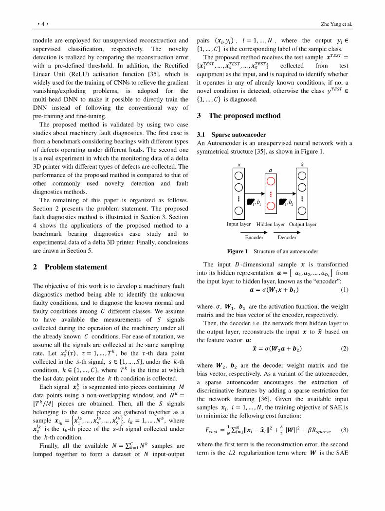
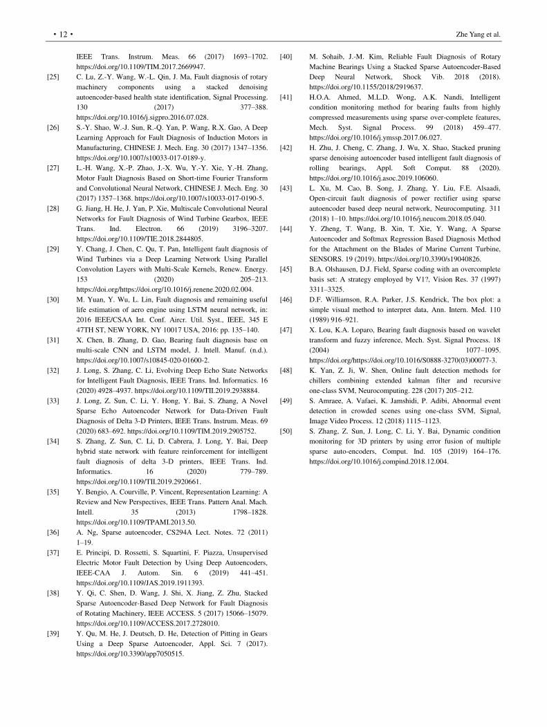
An Autoencoder is an unsupervised neural network with a
symmetrical structure [35], as shown in Figure 1.
...
... ...
x x
a
Encoder Decoder
1 1,bW
2 2,bW
Input layer Hidden layer Output layer
Figure 1 Structure of an autoencoder
The input 𝐷 -dimensional sample 𝒙 is transformed
into its hidden representation 𝒂 = [ 𝑎1, 𝑎2, … , 𝑎𝐷1] from
the input layer to hidden layer, known as the “encoder”: 𝒂 = 𝜎(𝑾1𝒙 + 𝒃1) (1)
where 𝜎, 𝑾1, 𝒃𝟏 are the activation function, the weight
matrix and the bias vector of the encoder, respectively.
Then, the decoder, i.e. the network from hidden layer to
the output layer, reconstructs the input 𝒙 to 𝒙 based on
the feature vector 𝒂: 𝒙 = 𝜎(𝑾2𝒂 + 𝒃2) (2)
where 𝑾2, 𝒃2 are the decoder weight matrix and the
bias vector, respectively. As a variant of the autoencoder,
a sparse autoencoder encourages the extraction of
discriminative features by adding a sparse restriction for
the network training [36]. Given the available input
samples 𝒙𝑖, 𝑖 = 1, … , 𝑁, the training objective of SAE is
to minimize the following cost function: 𝐹𝑐𝑜𝑠𝑡 = 1𝑁 ∑ ‖𝒙𝑖 − 𝒙𝑖‖2𝑁𝑖=1 + 𝜆2 ‖𝑾‖2 + 𝛽𝑅𝑠𝑝𝑎𝑟𝑠𝑒 (3)
where the first term is the reconstruction error, the second
term is the 𝐿2 regularization term where 𝑾 is the SAE
Sparse Autoencoder-based Multi-head Deep Neural Networks for Machinery Fault Diagnostics with Novelty Detection
·5·
weight matrix, 𝑅𝑠𝑝𝑎𝑟𝑠𝑒 is the sparsity regularization, and 𝜆 and 𝛽 are coefficients control the importance of the
corresponding terms.
It has been found that constraining hidden neurons to
be inactive most of the time makes them respond to
different patterns lying in the data, i.e. the extracted
features 𝒂 are discriminative [36]. Let ��𝑗 be the
average activation of the 𝑗-th hidden neuron of the SAE
hidden layer, considering all the input samples 𝒙𝑖 , 𝑖 =1, ⋯ , 𝑁: ��𝑗 = 1𝑁 ∑ 𝑎𝑖,𝑗𝑁𝑖=1 (4)
where 𝑎𝑖,𝑗 is the 𝑗 -th element of the 𝑖 -th hidden
representation 𝒂𝑖 , 𝑗 = 1, ⋯ , 𝐷1 . The sparsity
regularization in Eq. (3), 𝑅𝑠𝑝𝑎𝑟𝑠𝑒, is calculated using the
Kullback-Leibler (KL) divergence function to measure
whether ��𝑗 is close to a desired small sparsity proportion 𝑝: 𝑅𝑠𝑝𝑎𝑟𝑠𝑒 = ∑ KL(𝑝‖��𝑗)𝐷1𝑗=1 = ∑ [𝑝 log 𝑝𝑝𝑗 + (1 − 𝑝) log 1−𝑝1−𝑝𝑗]𝐷1𝑗=1 (5)
The KL function is zero when all ��𝑗 are equal to 𝑝 and
increases when they diverge.
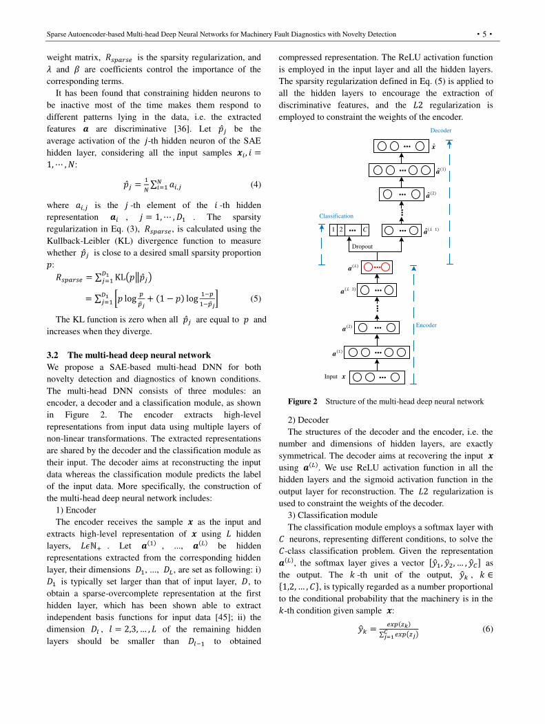
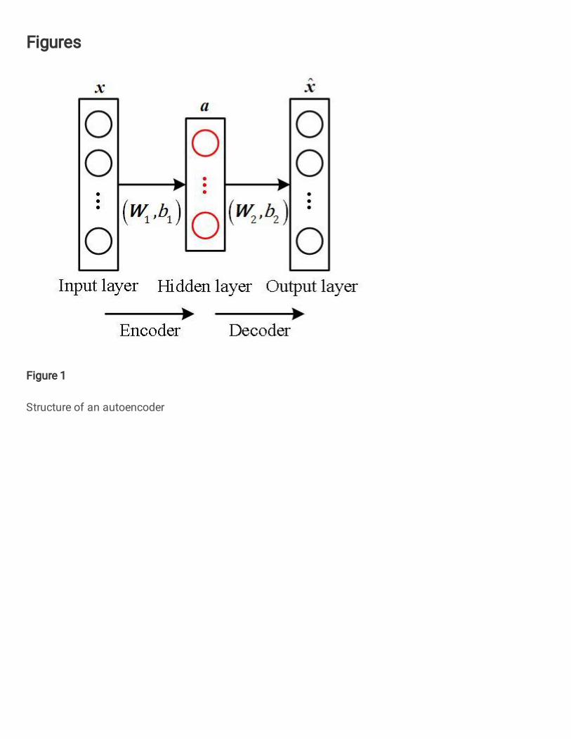
3.2 The multi-head deep neural network
We propose a SAE-based multi-head DNN for both
novelty detection and diagnostics of known conditions.
The multi-head DNN consists of three modules: an
encoder, a decoder and a classification module, as shown
in Figure 2. The encoder extracts high-level
representations from input data using multiple layers of
non-linear transformations. The extracted representations
are shared by the decoder and the classification module as
their input. The decoder aims at reconstructing the input
data whereas the classification module predicts the label
of the input data. More specifically, the construction of
the multi-head deep neural network includes:
1) Encoder
The encoder receives the sample 𝒙 as the input and
extracts high-level representation of 𝒙 using 𝐿 hidden
layers, 𝐿𝜖ℕ+ . Let 𝒂(1) , ..., 𝒂(𝐿) be hidden
representations extracted from the corresponding hidden
layer, their dimensions 𝐷1, ..., 𝐷𝐿 , are set as following: i) 𝐷1 is typically set larger than that of input layer, 𝐷, to
obtain a sparse-overcomplete representation at the first
hidden layer, which has been shown able to extract
independent basis functions for input data [45]; ii) the
dimension 𝐷𝑙 , 𝑙 = 2,3, … , 𝐿 of the remaining hidden
layers should be smaller than 𝐷𝑙−1 to obtained
compressed representation. The ReLU activation function
is employed in the input layer and all the hidden layers.
The sparsity regularization defined in Eq. (5) is applied to
all the hidden layers to encourage the extraction of
discriminative features, and the 𝐿2 regularization is
employed to constraint the weights of the encoder.
...x
(1)a
...
...
...
...
(2)a
( 1)La
( )La
...
...
...
...
...
...
x
Dropout
1 C2 ...
Encoder
Decoder
Classification
( 1)ˆ La
(2)a
(1)a
Input
Figure 2 Structure of the multi-head deep neural network
2) Decoder
The structures of the decoder and the encoder, i.e. the
number and dimensions of hidden layers, are exactly
symmetrical. The decoder aims at recovering the input 𝒙
using 𝒂(𝐿). We use ReLU activation function in all the
hidden layers and the sigmoid activation function in the
output layer for reconstruction. The 𝐿2 regularization is
used to constraint the weights of the decoder.
3) Classification module
The classification module employs a softmax layer with 𝐶 neurons, representing different conditions, to solve the 𝐶-class classification problem. Given the representation 𝒂(𝐿), the softmax layer gives a vector [��1, ��2, … , ��𝐶] as
the output. The 𝑘 -th unit of the output, ��𝑘 , 𝑘 ∈{1,2, … , 𝐶}, is typically regarded as a number proportional
to the conditional probability that the machinery is in the 𝑘-th condition given sample 𝒙: ��𝑘 = 𝑒𝑥𝑝(𝑧𝑘)∑ 𝑒𝑥𝑝(𝑧𝑗)𝐶𝑗=1 (6)
Zhe Yang et al.
·6·
where 0 ≤ ��𝑘 ≤ 1 , ∑ ��𝑘𝐶𝑘=1 = 1 and 𝑧𝑘 is the 𝑘 -th
output unit before applying the softmax activation
function: 𝑧𝑘 = 𝒘𝑘 ∙ 𝒂(𝐿) + 𝑏𝑘 (7)
where 𝒘𝑘 and 𝑏𝑘 are weights and bias of the 𝑘 -th
neuron of the softmax layer.
To prevent over-fitting, in the classification module, we
employ the dropout regularization on the hidden layer 𝒂(𝐿). Dropout randomly sets to zero a proportion 𝑝𝑑𝑟𝑜𝑝
of the hidden neurons during forward and
backpropagation [35]. Therefore, the following equation
is used for computing 𝑧𝑘 considering the dropout,
instead of using Eq. (7): 𝑧𝑘 = 𝒘𝑘 ∙ (𝒂(𝐿) ∘ 𝒓) + 𝑏𝑘 (8)
where ∘ is the element-wise multiplication operator and 𝒓 ∈ ℝ𝐷𝐿 is a ‘masking’ vector of Bernoulli random variables with probability 𝑝𝑑𝑟𝑜𝑝 of being 0. Gradients
are backpropagated only through the unmasked neurons.
To be associated with the neurons of the softmax layer,
in the training set (𝒙𝑖 , 𝑦𝑖), 𝑖 = 1, … , 𝑁, each label 𝑦𝑖 is
transformed into a one-hot 𝐶 -dimensional vector (𝑦𝑖,1, 𝑦𝑖,2, … , 𝑦𝑖,𝐶)𝑖=1,…,𝑁, where
𝑦𝑖,𝑘 = {1 𝑦𝑖 = 𝑘0 𝑜𝑡ℎ𝑒𝑟𝑤𝑖𝑠𝑒 , 𝑘 = 1, … , 𝐶 (9)
The training objective of the multi-head DNN over the
training set (𝒙𝑖 , 𝑦𝑖) , 𝑖 = 1, … , 𝑁 , is to minimize the
following cost function: 𝐹𝑐𝑜𝑠𝑡 = 𝜂1𝑁 ∑ ‖𝒙𝑖 − 𝒙𝑖‖2𝑁𝑖=1 + 𝜆2 ‖𝑾‖2
+𝛽 ∑ 𝑅𝑠𝑝𝑎𝑟𝑠𝑒(𝑗)𝐿𝑗=1 − 𝜂2𝑁 ∑ ∑ 𝑦𝑖,𝑘 log ��𝑖,𝑘𝐶𝑘=1𝑁𝑖=1 (10)
where the first term is the reconstruction error, the second
term is the 𝐿2 regularization term where 𝑾 is the
weight matrix of the whole multi-head DNN, 𝑅𝑠𝑝𝑎𝑟𝑠𝑒(𝑗) is
the sparsity regularization applied on the 𝑗-th hidden
layer of the encoder, the last term is the cross-entropy loss
measuring the performance of the classification module, 𝜆 , 𝛽 , 𝜂1 and 𝜂2 are coefficients controlling the
importance of the corresponding terms.
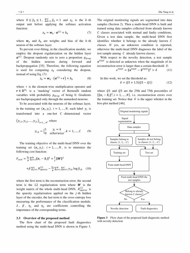
3.3 Overview of the proposed method
The flow chart of the proposed fault diagnostics
method using the multi-head DNN is shown in Figure 3.
The original monitoring signals are segmented into data
samples (Section 2). Then a multi-head DNN is built and
trained using data samples collected from already known 𝐶 classes associated with normal and faulty conditions.
Given a test data sample, the multi-head DNN first
identifies whether it belongs to the already known 𝐶
classes. If yes, an unknown condition is reported,
otherwise the multi-head DNN diagnoses the label of the
test sample among 𝐶 already known classes.
With respect to the novelty detection, a test sample 𝒙𝑇𝐸𝑆𝑇 is detected as unknown when the magnitude of its
reconstruction error is larger than a certain threshold 𝛿: 𝑒𝑇𝐸𝑆𝑇 = ‖𝒙𝑇𝐸𝑆𝑇 − 𝒙𝑇𝐸𝑆𝑇‖2 > 𝛿 (11)
In this work, we set the threshold as: 𝛿 = 𝑄3 + 1.5(𝑄3 − 𝑄1) (12)
where 𝑄1 and 𝑄3 are the 25th and 75th percentiles of {‖𝒙𝑖 − 𝒙𝑖‖2, 𝑖 = 1, … , 𝑁}, i.e. reconstruction errors over
the training set. Notice that 𝛿 is the upper whisker in the
box-plot method [46].
Original monitoring signals
Data samples
Training set
Signal
segmentation
Samples belong to
classes {1, 2,.., C}
Test set
Samples do not belong
to classes {1, 2,.., C}
Train multi-head DNN
Feed multi-head DNN the
test samples
Belong to already
known C classes?
Novelty detection Fault diagnostics
YesNo
Figure 3 Flow chart of the proposed fault diagnostic method
with novelty detection
Sparse Autoencoder-based Multi-head Deep Neural Networks for Machinery Fault Diagnostics with Novelty Detection
·7·
4 Experimental evaluations
The proposed method has been verified with respect to data
collected from a bearing fault benchmark, before its
application to the experimental data acquired on a delta 3D
printer. All computations have been performed using an
Intel Core i5-5200 CPU at 2.2 GHz processor with 4 GB
RAM in Python 3.6 environment.
4.1 Evaluation of the proposed method using
benchmark data
We consider the benchmark bearing diagnostics dataset
provided by the Case Western Reserve University, which
contains vibration data collected from an experimental rig
with defective bearings operating under four different loads
[47]. During the experiment, besides the normal condition,
three different kinds of fault, i.e. inner race fault, outer race
fault (at 6 o’clock) and ball fault, were introduced the drive-end bearing of the motor with fault diameters of 0.18
mm, 0.36 mm and 0.54 mm, respectively. Table 1 shows
the detailed description of the dataset. Vibration signals
were collected at sampling frequency 12KHz, by an
accelerometer attached through the magnetic base at the
drive-end.
Table 1 Bearing conditions with assigned labels
Bearing condition
Fault
diameter
(mm)
Label
/Class
Load
(hp)
Number
of samples
Normal - 1 0,1,2,3 1657
Inner Race Fault 0.18 2 0,1,2,3 476
Inner Race Fault 0.36 3 0,1,2,3 472
Inner Race Fault 0.54 4 0,1,2,3 474
Balls Fault 0.18 5 0,1,2,3 473
Balls Fault 0.36 6 0,1,2,3 475
Balls Fault 0.54 7 0,1,2,3 475
Outer Race Fault 0.18 8 0,1,2,3 475
Outer Race Fault 0.36 9 0,1,2,3 474
Outer Race Fault 0.54 10 0,1,2,3 476
The vibration signal of each condition is segmented
into samples using a non-overlapping fixed-length time
window containing 1024 data points. We implement Fast
Fourier Transformation (FFT) on each sample to get the
1024 Fourier amplitude coefficients. Since the
coefficients are symmetric, the first 512 coefficients are
used for each sample. The last column of Table 1 listed
the number of samples obtained for each bearing
condition.
We assume normal, inner race faults and balls faults are
already known conditions (classes 1-7), and the outer race
faults (classes 8-10) are unknown conditions. The training
set is composed of 70% of the data randomly selected
from classes 1-7, respectively. The remaining data of
classes 1-7 and all the data of classes 8-10 are used as the
test set. During the training of the multi-head DNN, 5% of
the training data is randomly selected as the validation set
to prevent the overfitting of the model. The developed
multi-head DNN is formed by an encoder with an input
layer of 𝐷 = 512 neurons and 𝐿 = 3 hidden layers of 𝐷1 = 600 , 𝐷2 = 100 , 𝐷3 = 10 neurons, a symmetric
decoder, and a classification module with a softmax layer
of 7 neurons associated with the known 1-7 classes in the
training set. The hyperparameters of the multi-head DNN
are set as following: 𝑝 = 0.05 , 𝜆 = 1𝑒 − 7 , 𝛽 = 1 , 𝜂1 = 80, 𝜂2 = 1 and 𝑝𝑑𝑟𝑜𝑝 = 0.3.
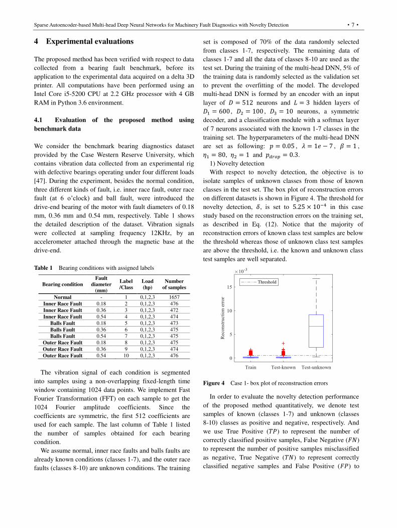
1) Novelty detection
With respect to novelty detection, the objective is to
isolate samples of unknown classes from those of known
classes in the test set. The box plot of reconstruction errors
on different datasets is shown in Figure 4. The threshold for
novelty detection, 𝛿, is set to 5.25 × 10⁻⁴ in this case
study based on the reconstruction errors on the training set,
as described in Eq. (12). Notice that the majority of
reconstruction errors of known class test samples are below
the threshold whereas those of unknown class test samples
are above the threshold, i.e. the known and unknown class
test samples are well separated.
Figure 4 Case 1- box plot of reconstruction errors
In order to evaluate the novelty detection performance
of the proposed method quantitatively, we denote test
samples of known (classes 1-7) and unknown (classes
8-10) classes as positive and negative, respectively. And
we use True Positive (𝑇𝑃) to represent the number of
correctly classified positive samples, False Negative (𝐹𝑁)
to represent the number of positive samples misclassified
as negative, True Negative (𝑇𝑁) to represent correctly
classified negative samples and False Positive (𝐹𝑃) to
Zhe Yang et al.
·8·
represent the number of negative samples misclassified as
positive. The novelty detection performance of the
developed multi-head DNN is evaluated considering the
True Positive Rate (𝑇𝑃𝑅), True Negative Rate (𝑇𝑁𝑅) and
the 𝐹1 score: 𝑇𝑟𝑢𝑒 𝑃𝑜𝑠𝑖𝑡𝑖𝑣𝑒 𝑅𝑎𝑡𝑒 (𝑇𝑃𝑅) = 𝑇𝑃𝑇𝑃+𝐹𝑁 (13)
𝑇𝑟𝑢𝑒 𝑁𝑒𝑔𝑎𝑡𝑖𝑣𝑒 𝑅𝑎𝑡𝑒 (𝑇𝑁𝑅) = 𝑇𝑁𝑇𝑁+𝐹𝑃 (14)
𝐹1 = 2𝑇𝑃2𝑇𝑃+𝐹𝑃+𝐹𝑁 (15)
The 𝑇𝑃𝑅 and 𝑇𝑁𝑅 are the proportions of correctly
classified positive and negative samples, respectively. The 𝐹1 score is widely used as a performance metric for
binary classification models, whose value ranges in [0,1] where the larger value indicates better performance.
The result of novelty detection of the proposed method
is shown in Table 2. The proposed method has been
compared with one-class SVM, which is a popular
one-class classification method aiming at constructing a
smooth boundary around the majority of probability mass
of data [48,49]. Since one-class SVM is a shallow model
which prefer low-dimensional input data, the 𝐷3 = 10
dimensional feature vectors 𝒂𝑖(3), 𝑖 = 1, … , 𝑁, extracted
by the encoder from the training set are used as its input.
The Radial Basis Function (RBF) kernel is used for
one-class SVM, and the parameter 𝜈, i.e. the assumed
proportion of negative samples in the training set, is set to
0.01, which has been optimized with the objective of
maximizing the 𝐹1 score by trial-and-error considering
as possible options {0,0.01, … ,0.2}, respectively.
As shown in Table 2, the proposed method provides a
satisfied 𝑇𝑁𝑅 = 98.53%, which means that nearly all
the samples of the unknown classes are correctly detected,
and the 𝑇𝑃𝑅 is 88.57% which means that most of the
samples of known classes can be identified. The 𝑇𝑃𝑅 of
one-class SVM is large whereas its 𝑇𝑁𝑅 is only 4.14%,
indicating that most of the samples of unknown classes
cannot be detected. Moreover, the proposed method gets a
larger 𝐹1 score which also indicates that its performance
is better than that of one-class SVM.
Table 2 Comparison of performance of novelty detection
The proposed
method
One-class SVM fed by
multi-head DNN features 𝑻𝑷𝑹 88.57% 97.69% 𝑻𝑵𝑹 98.53% 4.14% 𝑭𝟏 score 0.93 0.65
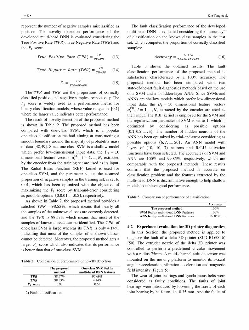
2) Fault classification
The fault classification performance of the developed
multi-head DNN is evaluated considering the “accuracy” of classification on the known class samples in the test
set, which computes the proportion of correctly classified
samples: 𝐴𝑐𝑐𝑢𝑟𝑎𝑐𝑦 = 𝑇𝑃+𝑇𝑁𝑇𝑃+𝐹𝑁+𝑇𝑁+𝐹𝑃 (16)
Table 3 shows the obtained results. The fault
classification performance of the proposed method is
satisfactory, characterized by a 100% accuracy. The
proposed method has been compared with two
state-of-the-art fault diagnostics methods based on the use
of a SVM and a 1-hidden-layer ANN. Since SVMs and
ANNs are shallow models which prefer low-dimensional
input data, the 𝐷3 = 10 dimensional feature vectors 𝒂𝑖(3), 𝑖 = 1, … , 𝑁, extracted by the encoder are used as
their input. The RBF kernel is employed for the SVM and
the regularization parameter of SVM is set to 1, which is
optimized by considering as possible options {0.1, 0.2, … , 5}. The number of hidden neurons of the
ANN has been optimized by trial-and-error considering as
possible options {6, 7, … , 50} . An ANN model with
layers of (10, 10, 7) neurons and ReLU activation
functions have been selected. The accuracies of SVM and
ANN are 100% and 99.85%, respectively, which are
comparable with the proposed methods. These results
confirm that the proposed method is accurate on
classification problem and the features extracted by the
multi-head DNN is discriminative enough to help shallow
models to achieve good performance.
Table 3 Comparison of performance of classification
Accuracy
The proposed method 100%
SVM fed by multi-head DNN features 100%
ANN fed by multi-head DNN features 99.85%
4.2 Experiment evaluation for 3D printer diagnostics
In this Section, the proposed method is applied to
diagnose the fault of a delta 3D printer (SLD-BL600-6)
[50]. The extruder nozzle of the delta 3D printer was
controlled to perform a predefined circular movement
with a radius 75mm. A multi-channel attitude sensor was
mounted on the moving platform to monitor its 3-axial
angular acceleration, vibration acceleration and magnetic
field intensity (Figure 5).
The wear of joint bearings and synchronous belts were
considered as faulty conditions. The faults of joint
bearings were introduced by loosening the screw of each
joint bearing by half-turn, i.e. 0.35 mm. And the faults of
Sparse Autoencoder-based Multi-head Deep Neural Networks for Machinery Fault Diagnostics with Novelty Detection
·9·
synchronous belts were injected by relaxing the length of
two teeth, i.e. 3 mm, for each belt. In each fault condition,
we consider exclusively the fault of one joint bearing or
one synchronous belt. As listed in Table 4, 15 faulty
conditions are simulated in total, including faults of 12
joint bearings and 3 synchronous belts. Printing tests were
performed under these faulty conditions and we found
that the printing quality of the 3D printer was affected
seriously. Figure 6 shows examples of the normal mode
and faulty mode of the joint bearing and synchronous belt,
respectively.
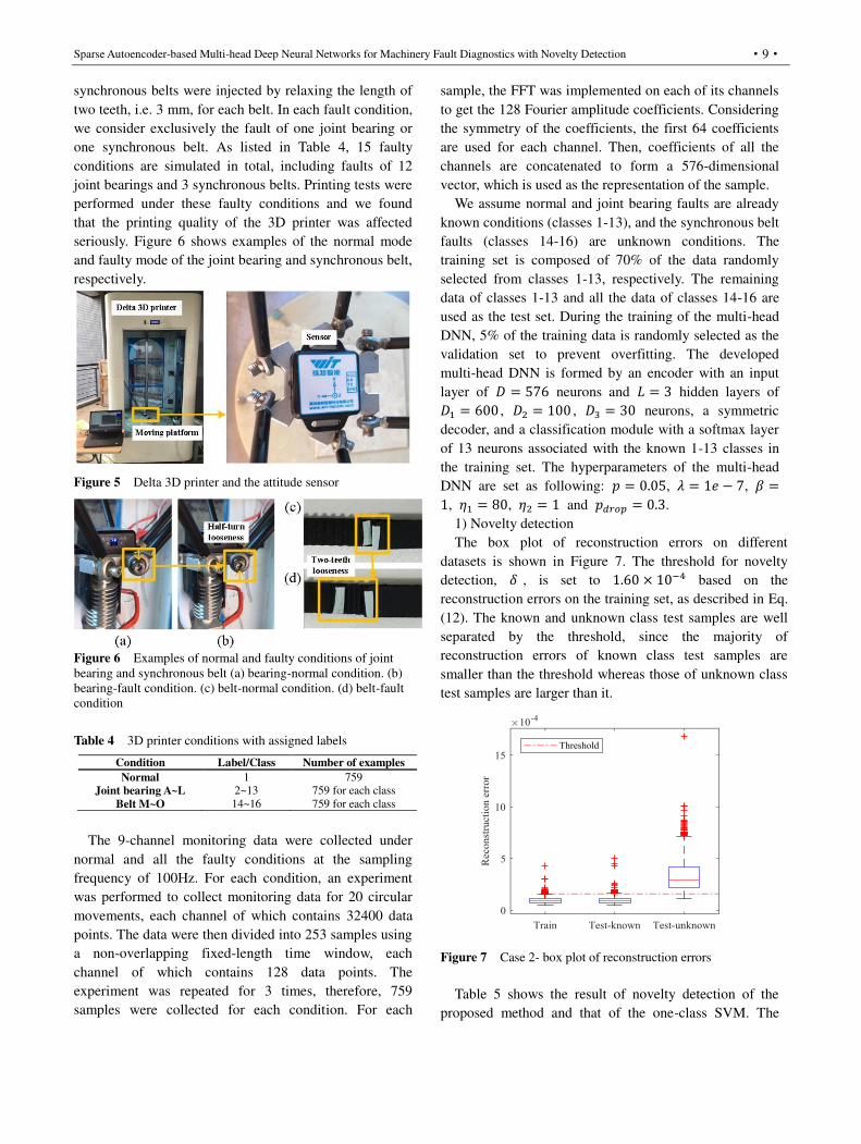
Figure 5 Delta 3D printer and the attitude sensor
Figure 6 Examples of normal and faulty conditions of joint
bearing and synchronous belt (a) bearing-normal condition. (b)
bearing-fault condition. (c) belt-normal condition. (d) belt-fault
condition
Table 4 3D printer conditions with assigned labels
Condition Label/Class Number of examples
Normal 1 759
Joint bearing A~L 2~13 759 for each class
Belt M~O 14~16 759 for each class
The 9-channel monitoring data were collected under
normal and all the faulty conditions at the sampling
frequency of 100Hz. For each condition, an experiment
was performed to collect monitoring data for 20 circular
movements, each channel of which contains 32400 data
points. The data were then divided into 253 samples using
a non-overlapping fixed-length time window, each
channel of which contains 128 data points. The
experiment was repeated for 3 times, therefore, 759
samples were collected for each condition. For each
sample, the FFT was implemented on each of its channels
to get the 128 Fourier amplitude coefficients. Considering
the symmetry of the coefficients, the first 64 coefficients
are used for each channel. Then, coefficients of all the
channels are concatenated to form a 576-dimensional
vector, which is used as the representation of the sample.
We assume normal and joint bearing faults are already
known conditions (classes 1-13), and the synchronous belt
faults (classes 14-16) are unknown conditions. The
training set is composed of 70% of the data randomly
selected from classes 1-13, respectively. The remaining
data of classes 1-13 and all the data of classes 14-16 are
used as the test set. During the training of the multi-head
DNN, 5% of the training data is randomly selected as the
validation set to prevent overfitting. The developed
multi-head DNN is formed by an encoder with an input
layer of 𝐷 = 576 neurons and 𝐿 = 3 hidden layers of 𝐷1 = 600 , 𝐷2 = 100 , 𝐷3 = 30 neurons, a symmetric
decoder, and a classification module with a softmax layer
of 13 neurons associated with the known 1-13 classes in
the training set. The hyperparameters of the multi-head
DNN are set as following: 𝑝 = 0.05, 𝜆 = 1𝑒 − 7, 𝛽 =1, 𝜂1 = 80, 𝜂2 = 1 and 𝑝𝑑𝑟𝑜𝑝 = 0.3.
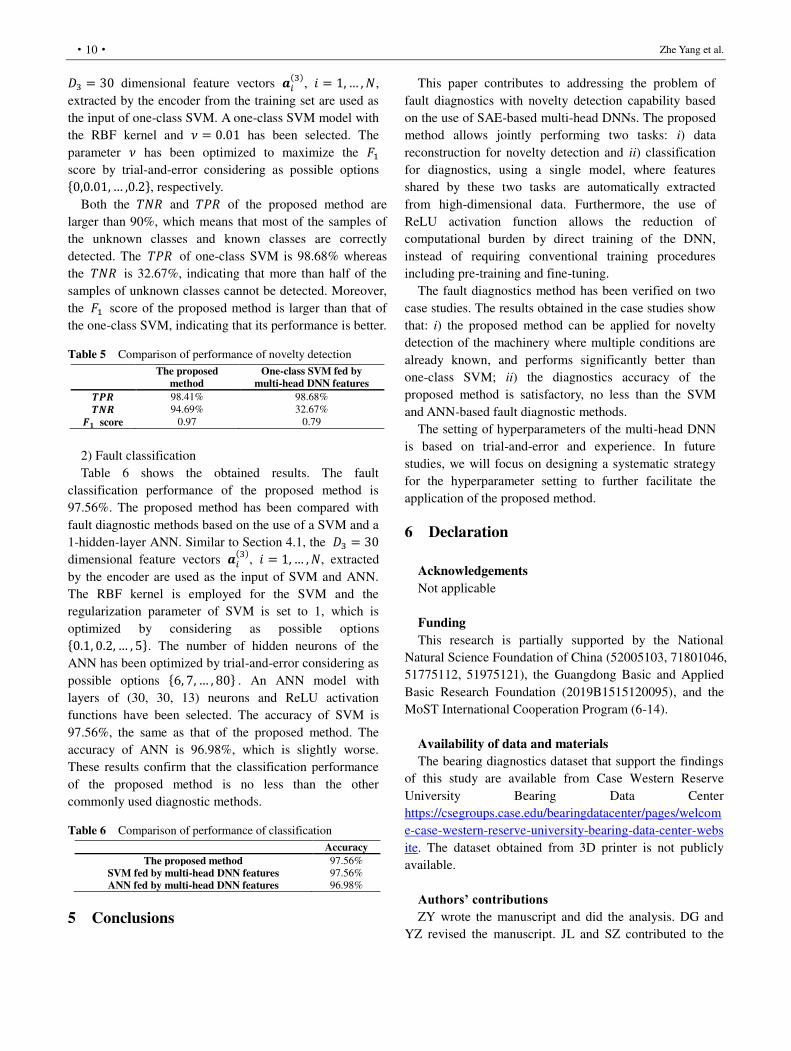
1) Novelty detection
The box plot of reconstruction errors on different
datasets is shown in Figure 7. The threshold for novelty
detection, 𝛿 , is set to 1.60 × 10⁻⁴ based on the
reconstruction errors on the training set, as described in Eq.
(12). The known and unknown class test samples are well
separated by the threshold, since the majority of
reconstruction errors of known class test samples are
smaller than the threshold whereas those of unknown class
test samples are larger than it.
Figure 7 Case 2- box plot of reconstruction errors
Table 5 shows the result of novelty detection of the
proposed method and that of the one-class SVM. The
Zhe Yang et al.
·10· 𝐷3 = 30 dimensional feature vectors 𝒂𝑖(3), 𝑖 = 1, … , 𝑁,
extracted by the encoder from the training set are used as
the input of one-class SVM. A one-class SVM model with
the RBF kernel and 𝜈 = 0.01 has been selected. The
parameter 𝜈 has been optimized to maximize the 𝐹1
score by trial-and-error considering as possible options {0,0.01, … ,0.2}, respectively.
Both the 𝑇𝑁𝑅 and 𝑇𝑃𝑅 of the proposed method are
larger than 90%, which means that most of the samples of
the unknown classes and known classes are correctly
detected. The 𝑇𝑃𝑅 of one-class SVM is 98.68% whereas
the 𝑇𝑁𝑅 is 32.67%, indicating that more than half of the
samples of unknown classes cannot be detected. Moreover,
the 𝐹1 score of the proposed method is larger than that of
the one-class SVM, indicating that its performance is better.
Table 5 Comparison of performance of novelty detection
The proposed
method
One-class SVM fed by
multi-head DNN features 𝑻𝑷𝑹 98.41% 98.68% 𝑻𝑵𝑹 94.69% 32.67% 𝑭𝟏 score 0.97 0.79
2) Fault classification
Table 6 shows the obtained results. The fault
classification performance of the proposed method is
97.56%. The proposed method has been compared with
fault diagnostic methods based on the use of a SVM and a
1-hidden-layer ANN. Similar to Section 4.1, the 𝐷3 = 30
dimensional feature vectors 𝒂𝑖(3), 𝑖 = 1, … , 𝑁, extracted
by the encoder are used as the input of SVM and ANN.
The RBF kernel is employed for the SVM and the
regularization parameter of SVM is set to 1, which is
optimized by considering as possible options {0.1, 0.2, … , 5}. The number of hidden neurons of the
ANN has been optimized by trial-and-error considering as
possible options {6, 7, … , 80} . An ANN model with
layers of (30, 30, 13) neurons and ReLU activation
functions have been selected. The accuracy of SVM is
97.56%, the same as that of the proposed method. The
accuracy of ANN is 96.98%, which is slightly worse.
These results confirm that the classification performance
of the proposed method is no less than the other
commonly used diagnostic methods.
Table 6 Comparison of performance of classification
Accuracy
The proposed method 97.56%
SVM fed by multi-head DNN features 97.56%
ANN fed by multi-head DNN features 96.98%
5 Conclusions
This paper contributes to addressing the problem of
fault diagnostics with novelty detection capability based
on the use of SAE-based multi-head DNNs. The proposed
method allows jointly performing two tasks: i) data
reconstruction for novelty detection and ii) classification
for diagnostics, using a single model, where features
shared by these two tasks are automatically extracted
from high-dimensional data. Furthermore, the use of
ReLU activation function allows the reduction of
computational burden by direct training of the DNN,
instead of requiring conventional training procedures
including pre-training and fine-tuning.
The fault diagnostics method has been verified on two
case studies. The results obtained in the case studies show
that: i) the proposed method can be applied for novelty
detection of the machinery where multiple conditions are
already known, and performs significantly better than
one-class SVM; ii) the diagnostics accuracy of the
proposed method is satisfactory, no less than the SVM
and ANN-based fault diagnostic methods.
The setting of hyperparameters of the multi-head DNN
is based on trial-and-error and experience. In future
studies, we will focus on designing a systematic strategy
for the hyperparameter setting to further facilitate the
application of the proposed method.
6 Declaration
Acknowledgements
Not applicable
Funding
This research is partially supported by the National
Natural Science Foundation of China (52005103, 71801046,
51775112, 51975121), the Guangdong Basic and Applied
Basic Research Foundation (2019B1515120095), and the
MoST International Cooperation Program (6-14).
Availability of data and materials
The bearing diagnostics dataset that support the findings
of this study are available from Case Western Reserve
University Bearing Data Center
https://csegroups.case.edu/bearingdatacenter/pages/welcom
e-case-western-reserve-university-bearing-data-center-webs
ite. The dataset obtained from 3D printer is not publicly
available.
Authors’ contributions
ZY wrote the manuscript and did the analysis. DG and
YZ revised the manuscript. JL and SZ contributed to the
Sparse Autoencoder-based Multi-head Deep Neural Networks for Machinery Fault Diagnostics with Novelty Detection
·11·
experiments. CL was in charge of the whole work. All
authors read and approved
Competing interests
The authors declare no competing financial interests.
Consent for publication
Not applicable
Ethics approval and consent to participate
Not applicable
References
[1] E. Zio, Some Challenges and Opportunities in Reliability
Engineering, IEEE Trans. Reliab. 65 (2016) 1769–1782.
https://doi.org/10.1109/TR.2016.2591504.
[2] D. Wang, K.-L. Tsui, Q. Miao, Prognostics and Health
Management: A Review of Vibration Based Bearing and Gear
Health Indicators, IEEE ACCESS. 6 (2018).
https://doi.org/10.1109/ACCESS.2017.2774261.
[3] J. Zhong, J. Long, S. Zhang, C. Li, Flexible kurtogram for
extracting repetitive transients for prognostics and health
management of rotating components, IEEE Access. 7 (2019)
55631–55639. https://doi.org/10.1109/ACCESS.2019.2912716.
[4] P. Baraldi, F. Cadini, F. Mangili, E. Zio, Model-based and
data-driven prognostics under different available information,
PROBABILISTIC Eng. Mech. 32 (2013) 66–79.
https://doi.org/10.1016/j.probengmech.2013.01.003.
[5] H. Wang, J. Xu, R. Yan, R.X. Gao, A New Intelligent Bearing
Fault Diagnosis Method Using SDP Representation and
SE-CNN, IEEE Trans. Instrum. Meas. 69 (2020) 2377–2389.
https://doi.org/10.1109/TIM.2019.2956332.
[6] W. Chine, A. Mellit, V. Lughi, A. Malek, G. Sulligoi, A.M.
Pavan, A novel fault diagnosis technique for photovoltaic
systems based on artificial neural networks, Renew. ENERGY.
90 (2016) 501–512.
https://doi.org/10.1016/j.renene.2016.01.036.
[7] H. Malik, Y. Pandya, A. Parashar, R. Sharma, Feature
Extraction Using EMD and Classifier Through Artificial Neural
Networks for Gearbox Fault Diagnosis, in: Malik, H and
Srivastava, S and Sood, YR and Ahmad, A (Ed.), Appl. Artif.
Intell. Tech. Eng. VOL 2, SPRINGER INTERNATIONAL
PUBLISHING AG, GEWERBESTRASSE 11, CHAM,
CH-6330, SWITZERLAND, 2019: pp. 309–317.
https://doi.org/10.1007/978-981-13-1822-1_28.
[8] K. He, Z. Yang, Y. Bai, J. Long, C. Li, Intelligent fault
diagnosis of delta 3D printers using attitude sensors based on
support vector machines, Sensors (Switzerland). 18 (2018).
https://doi.org/10.3390/s18041298.
[9] X. Li, S. Wu, X. Li, H. Yuan, D. Zhao, Particle Swarm
Optimization-Support Vector Machine Model for Machinery
Fault Diagnoses in High-Voltage Circuit Breakers, CHINESE J.
Mech. Eng. 33 (2020).
https://doi.org/10.1186/s10033-019-0428-5.
[10] G. Liu, H. Li, W. Liu, Bearing Fault Detection in Varying
Operational Conditions based on Empirical Mode
Decomposition and Random Forest, in: Ding, P and Li, C and
Sanchez, RV and Yang, S (Ed.), 2018 Progn. Syst. Heal. Manag.
Conf. (PHM-CHONGQING 2018), IEEE, 345 E 47TH ST,
NEW YORK, NY 10017 USA, 2018: pp. 851–854.
https://doi.org/10.1109/PHM-Chongqing.2018.00152.
[11] Y. Hu, S. Thang, A. Jiang, L. Thang, W. Jiang, J. Li, A New
Method of Wind Turbine Bearing Fault Diagnosis Based on
Multi-Masking Empirical Mode Decomposition and Fuzzy
C-Means Clustering, CHINESE J. Mech. Eng. 32 (2019).
https://doi.org/10.1186/s10033-019-0356-4.
[12] P. Baraldi, F. Cannarile, F. Di Maio, E. Zio, Hierarchical
k-nearest neighbours classification and binary differential
evolution for fault diagnostics of automotive bearings operating
under variable conditions, Eng. Appl. Artif. Intell. 56 (2016)
1–13. https://doi.org/10.1016/j.engappai.2016.08.011.
[13] J. Yu, M. Bai, G. Wang, X. Shi, Fault diagnosis of planetary
gearbox with incomplete information using assignment
reduction and flexible naive Bayesian classifier, J. Mech. Sci.
Technol. 32 (2018) 37–47.
https://doi.org/10.1007/s12206-017-1205-y.
[14] A. Yang, Y. Wang, Y. Zi, T.W.S. Chow, An Enhanced Trace
Ratio Linear Discriminant Analysis for Fault Diagnosis: An
Illustrated Example Using HDD Data, IEEE Trans. Instrum.
Meas. 68 (2019) 4629–4639.
https://doi.org/10.1109/TIM.2019.2900885.
[15] M. Tan, J. Li, X. Chen, X. Cheng, Power Grid Fault Diagnosis
Method Using Intuitionistic Fuzzy Petri Nets Based on Time
Series Matching, Complexity. 2019 (2019).
https://doi.org/10.1155/2019/7890652.
[16] K. Li, L. Su, J. Wu, H. Wang, P. Chen, A Rolling Bearing Fault
Diagnosis Method Based on Variational Mode Decomposition
and an Improved Kernel Extreme Learning Machine, Appl. Sci.
7 (2017). https://doi.org/10.3390/app7101004.
[17] S. Khan, T. Yairi, A review on the application of deep learning
in system health management, Mech. Syst. Signal Process. 107
(2018) 241–265. https://doi.org/10.1016/j.ymssp.2017.11.024.
[18] R. Zhao, R. Yan, Z. Chen, K. Mao, P. Wang, R.X. Gao, Deep
learning and its applications to machine health monitoring,
Mech. Syst. Signal Process. 115 (2019) 213–237.
https://doi.org/10.1016/j.ymssp.2018.05.050.
[19] C. Li, S. Zhang, Y. Qin, E. Estupinan, A systematic review of
deep transfer learning for machinery fault diagnosis,
Neurocomputing. 407 (2020) 121–135.
https://doi.org/https://doi.org/10.1016/j.neucom.2020.04.045.
[20] R. Yan, F. Shen, C. Sun, X. Chen, Knowledge Transfer for
Rotary Machine Fault Diagnosis, IEEE Sens. J. 20 (2020)
8374–8393. https://doi.org/10.1109/JSEN.2019.2949057.
[21] Y. LeCun, Y. Bengio, G. Hinton, Deep learning, Nature. 521
(2015) 436–444. https://doi.org/10.1038/nature14539.
[22] J. Dai, J. Tang, S. Huang, Y. Wang, Signal-Based Intelligent
Hydraulic Fault Diagnosis Methods: Review and Prospects,
CHINESE J. Mech. Eng. 32 (2019).
https://doi.org/10.1186/s10033-019-0388-9.
[23] F. Jia, Y. Lei, J. Lin, X. Zhou, N. Lu, Deep neural networks: A
promising tool for fault characteristic mining and intelligent
diagnosis of rotating machinery with massive data, Mech. Syst.
Signal Process. 72–73 (2016) 303–315.
https://doi.org/10.1016/j.ymssp.2015.10.025.
[24] Z. Chen, W. Li, Multisensor Feature Fusion for Bearing Fault
Diagnosis Using Sparse Autoencoder and Deep Belief Network,
Zhe Yang et al.
·12·
IEEE Trans. Instrum. Meas. 66 (2017) 1693–1702.
https://doi.org/10.1109/TIM.2017.2669947.
[25] C. Lu, Z.-Y. Wang, W.-L. Qin, J. Ma, Fault diagnosis of rotary
machinery components using a stacked denoising
autoencoder-based health state identification, Signal Processing.
130 (2017) 377–388.
https://doi.org/10.1016/j.sigpro.2016.07.028.
[26] S.-Y. Shao, W.-J. Sun, R.-Q. Yan, P. Wang, R.X. Gao, A Deep
Learning Approach for Fault Diagnosis of Induction Motors in
Manufacturing, CHINESE J. Mech. Eng. 30 (2017) 1347–1356.
https://doi.org/10.1007/s10033-017-0189-y.
[27] L.-H. Wang, X.-P. Zhao, J.-X. Wu, Y.-Y. Xie, Y.-H. Zhang,
Motor Fault Diagnosis Based on Short-time Fourier Transform
and Convolutional Neural Network, CHINESE J. Mech. Eng. 30
(2017) 1357–1368. https://doi.org/10.1007/s10033-017-0190-5.
[28] G. Jiang, H. He, J. Yan, P. Xie, Multiscale Convolutional Neural
Networks for Fault Diagnosis of Wind Turbine Gearbox, IEEE
Trans. Ind. Electron. 66 (2019) 3196–3207.
https://doi.org/10.1109/TIE.2018.2844805.
[29] Y. Chang, J. Chen, C. Qu, T. Pan, Intelligent fault diagnosis of
Wind Turbines via a Deep Learning Network Using Parallel
Convolution Layers with Multi-Scale Kernels, Renew. Energy.
153 (2020) 205–213.
https://doi.org/https://doi.org/10.1016/j.renene.2020.02.004.
[30] M. Yuan, Y. Wu, L. Lin, Fault diagnosis and remaining useful
life estimation of aero engine using LSTM neural network, in:
2016 IEEE/CSAA Int. Conf. Aircr. Util. Syst., IEEE, 345 E
47TH ST, NEW YORK, NY 10017 USA, 2016: pp. 135–140.
[31] X. Chen, B. Zhang, D. Gao, Bearing fault diagnosis base on
multi-scale CNN and LSTM model, J. Intell. Manuf. (n.d.).
https://doi.org/10.1007/s10845-020-01600-2.
[32] J. Long, S. Zhang, C. Li, Evolving Deep Echo State Networks
for Intelligent Fault Diagnosis, IEEE Trans. Ind. Informatics. 16
(2020) 4928–4937. https://doi.org/10.1109/TII.2019.2938884.
[33] J. Long, Z. Sun, C. Li, Y. Hong, Y. Bai, S. Zhang, A Novel
Sparse Echo Autoencoder Network for Data-Driven Fault
Diagnosis of Delta 3-D Printers, IEEE Trans. Instrum. Meas. 69
(2020) 683–692. https://doi.org/10.1109/TIM.2019.2905752.
[34] S. Zhang, Z. Sun, C. Li, D. Cabrera, J. Long, Y. Bai, Deep
hybrid state network with feature reinforcement for intelligent
fault diagnosis of delta 3-D printers, IEEE Trans. Ind.
Informatics. 16 (2020) 779–789.
https://doi.org/10.1109/TII.2019.2920661.
[35] Y. Bengio, A. Courville, P. Vincent, Representation Learning: A
Review and New Perspectives, IEEE Trans. Pattern Anal. Mach.
Intell. 35 (2013) 1798–1828.
https://doi.org/10.1109/TPAMI.2013.50.
[36] A. Ng, Sparse autoencoder, CS294A Lect. Notes. 72 (2011)
1–19.
[37] E. Principi, D. Rossetti, S. Squartini, F. Piazza, Unsupervised
Electric Motor Fault Detection by Using Deep Autoencoders,
IEEE-CAA J. Autom. Sin. 6 (2019) 441–451.
https://doi.org/10.1109/JAS.2019.1911393.
[38] Y. Qi, C. Shen, D. Wang, J. Shi, X. Jiang, Z. Zhu, Stacked
Sparse Autoencoder-Based Deep Network for Fault Diagnosis
of Rotating Machinery, IEEE ACCESS. 5 (2017) 15066–15079.
https://doi.org/10.1109/ACCESS.2017.2728010.
[39] Y. Qu, M. He, J. Deutsch, D. He, Detection of Pitting in Gears
Using a Deep Sparse Autoencoder, Appl. Sci. 7 (2017).
https://doi.org/10.3390/app7050515.
[40] M. Sohaib, J.-M. Kim, Reliable Fault Diagnosis of Rotary
Machine Bearings Using a Stacked Sparse Autoencoder-Based
Deep Neural Network, Shock Vib. 2018 (2018).
https://doi.org/10.1155/2018/2919637.
[41] H.O.A. Ahmed, M.L.D. Wong, A.K. Nandi, Intelligent
condition monitoring method for bearing faults from highly
compressed measurements using sparse over-complete features,
Mech. Syst. Signal Process. 99 (2018) 459–477.
https://doi.org/10.1016/j.ymssp.2017.06.027.
[42] H. Zhu, J. Cheng, C. Zhang, J. Wu, X. Shao, Stacked pruning
sparse denoising autoencoder based intelligent fault diagnosis of
rolling bearings, Appl. Soft Comput. 88 (2020).
https://doi.org/10.1016/j.asoc.2019.106060.
[43] L. Xu, M. Cao, B. Song, J. Zhang, Y. Liu, F.E. Alsaadi,
Open-circuit fault diagnosis of power rectifier using sparse
autoencoder based deep neural network, Neurocomputing. 311
(2018) 1–10. https://doi.org/10.1016/j.neucom.2018.05.040.
[44] Y. Zheng, T. Wang, B. Xin, T. Xie, Y. Wang, A Sparse
Autoencoder and Softmax Regression Based Diagnosis Method
for the Attachment on the Blades of Marine Current Turbine,
SENSORS. 19 (2019). https://doi.org/10.3390/s19040826.
[45] B.A. Olshausen, D.J. Field, Sparse coding with an overcomplete
basis set: A strategy employed by V1?, Vision Res. 37 (1997)
3311–3325.
[46] D.F. Williamson, R.A. Parker, J.S. Kendrick, The box plot: a
simple visual method to interpret data, Ann. Intern. Med. 110
(1989) 916–921.
[47] X. Lou, K.A. Loparo, Bearing fault diagnosis based on wavelet
transform and fuzzy inference, Mech. Syst. Signal Process. 18
(2004) 1077–1095.
https://doi.org/https://doi.org/10.1016/S0888-3270(03)00077-3.
[48] K. Yan, Z. Ji, W. Shen, Online fault detection methods for
chillers combining extended kalman filter and recursive
one-class SVM, Neurocomputing. 228 (2017) 205–212.
[49] S. Amraee, A. Vafaei, K. Jamshidi, P. Adibi, Abnormal event
detection in crowded scenes using one-class SVM, Signal,
Image Video Process. 12 (2018) 1115–1123.
[50] S. Zhang, Z. Sun, J. Long, C. Li, Y. Bai, Dynamic condition
monitoring for 3D printers by using error fusion of multiple
sparse auto-encoders, Comput. Ind. 105 (2019) 164–176.
https://doi.org/10.1016/j.compind.2018.12.004.
Figures
Figure 1
Structure of an autoencoder
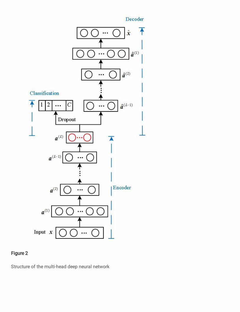
Figure 2
Structure of the multi-head deep neural network
Figure 3
Flow chart of the proposed fault diagnostic method with novelty detection
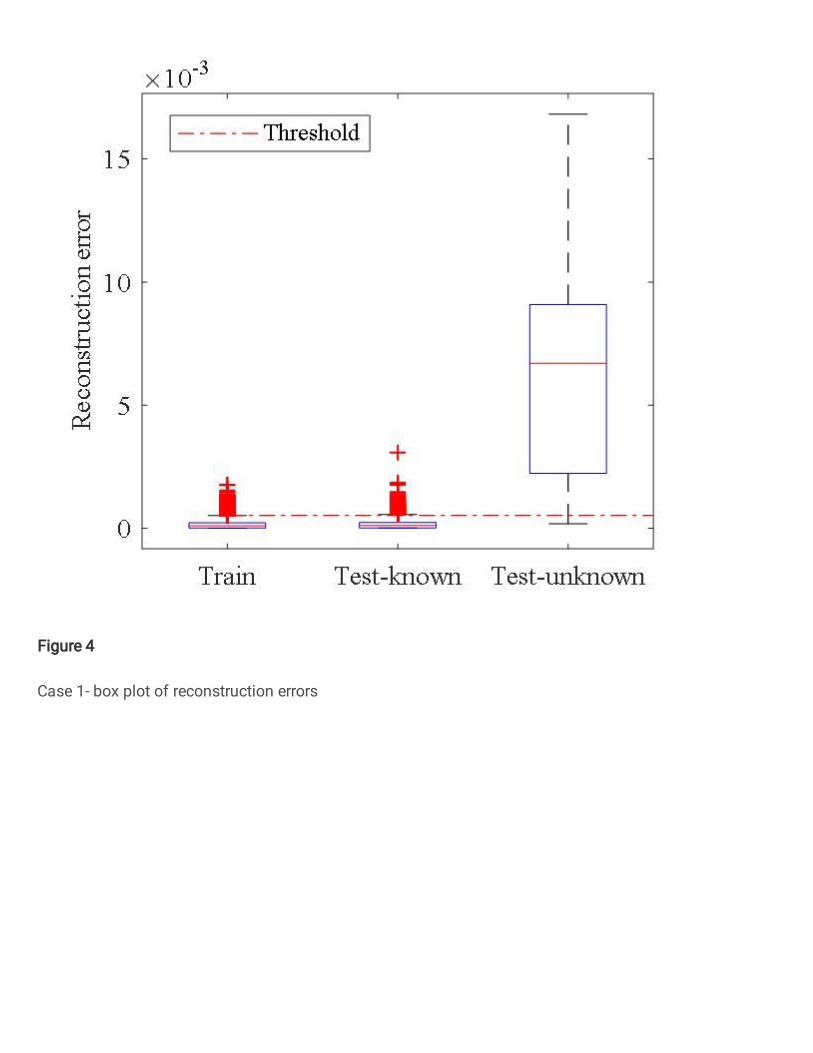
Figure 4
Case 1- box plot of reconstruction errors
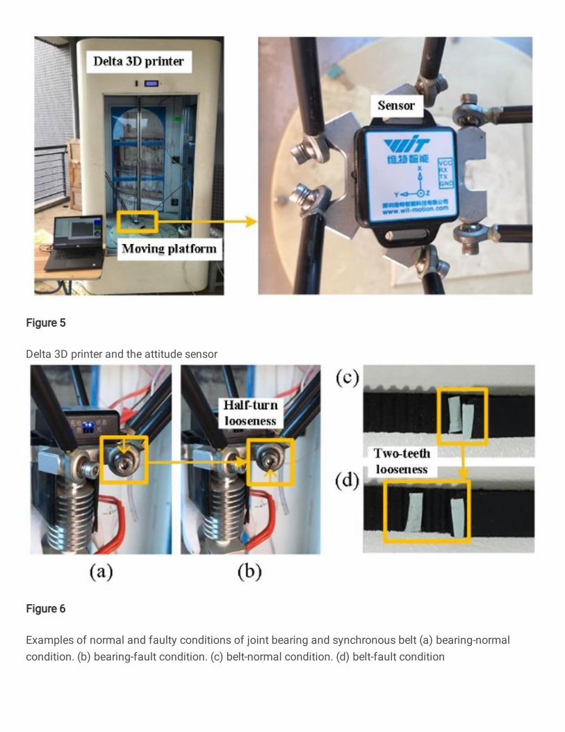
Figure 5
Delta 3D printer and the attitude sensor
Figure 6
Examples of normal and faulty conditions of joint bearing and synchronous belt (a) bearing-normalcondition. (b) bearing-fault condition. (c) belt-normal condition. (d) belt-fault condition
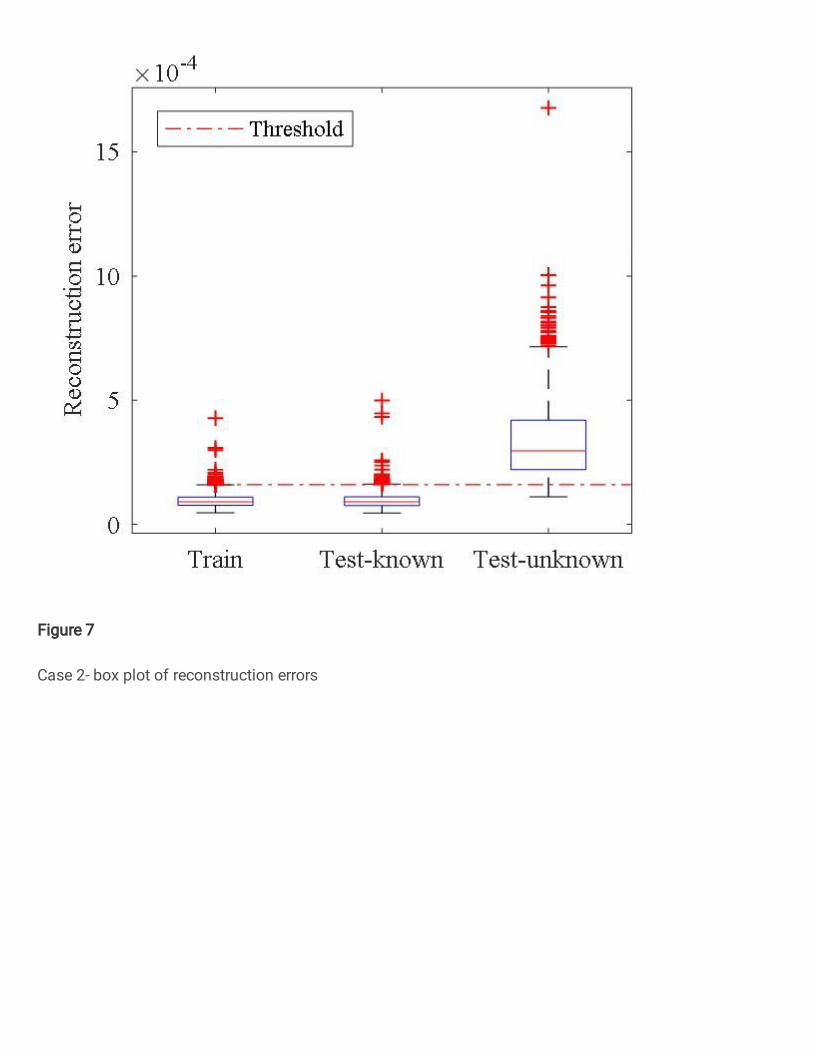
Figure 7
Case 2- box plot of reconstruction errors