A salt tracer test monitored with surface ERT to detect preferential flowand transport paths in fractured/karstified limestones

Tanguy Robert1, David Caterina1, John Deceuster2, Olivier Kaufmann2, and Frédéric Nguyen3

ABSTRACT

In hard-rock aquifers, fractured zones constitute adequatedrinking water exploitation areas but also potential contamina-tion paths. One critical issue in hydrogeological research is toidentify, characterize, and monitor such fractured zones at a re-presentative scale. A tracer test monitored with surface electricalresistivity tomography (ERT) could help by delineating suchpreferential flow paths and estimating dynamic properties ofthe aquifer. However, multiple challenges exist including thelower resolution of surface ERT compared with crossholeERT, the finite time that is needed to complete an entire dataacquisition, and the strong dilution effects. We conducted a nat-ural gradient salt tracer test in fractured limestones. To accountfor the high transport velocity, we injected the salt tracer con-tinuously for four hours at a depth of 18 m. We monitored itspropagation with two parallel ERT profiles perpendicular to the

groundwater flow direction. Concerning the data acquisition, wealways focused on data quality over temporal resolution. Weperformed the experiment twice to prove its reproducibilityby increasing the salt concentration in the injected solution(from 38 to 154 g∕L). Our research focused on how we facedevery challenge to delineate a preferential flow and solutetransport path in a typical calcareous valley of southern Belgiumand on the estimation of the transport velocity (more than10 m∕hour). In this complex environment, we imaged a cleartracer arrival in both ERT profiles and for both tests. Applyingfilters (with a cutoff on the relative sensitivity matrix and on thebackground-resistivity changes) was helpful to isolate the pre-ferential flow path from artifacts. Regarding our findings, ourapproach could be improved to perform a more quantitativeexperiment. With a higher temporal resolution, the estimatedvalue of the transport velocity could be narrowed, allowingestimation of the percentage of tracer recovery.

INTRODUCTION

Fractured zones are extremely important to identify and to char-acterize because they are preferential groundwater flow and solutetransport paths (Berkowitz, 2002). They constitute adequate drink-ing water exploitation areas but also potential contamination paths.Important issues in hydrogeological research, as was pointed out byPost (2005), are not so much the mathematical descriptions of pro-cesses or techniques but their applications to real-world data andcases. In this framework, innovative techniques or methodologiesare needed to locate and characterize fractured zones in hard-rockaquifers as well as to monitor groundwater flow or solute transportthrough them.

Numerous field techniques and methodologies exist to obtain hy-drogeological information about fractured aquifers. Classical pump-ing tests allow estimating the hydraulic conductivity in an areaaround the well and evaluating the absence or presence of hydrau-lically conductive fractures. These tests are useful but not flawless(Wu et al., 2005) because they depend on strong assumptions suchas Theis’ homogeneous aquifer assumption (Fetter, 2001). Pumpingtests evolved into hydraulic tomography which allows obtaininghigh resolution images of the hydraulic conductivity distribution(Yeh and Liu, 2000; Liu et al., 2002; Zhu and Yeh, 2005; Illmanand Tartakovsky, 2006; Zhu and Yeh, 2006; Hao et al., 2008; Illmanet al., 2008; Yin and Illman, 2009). However, this method requiresseveral wells and prior knowledge about the location of fractures.

Manuscript received by the Editor 19 August 2011; revised manuscript received 16 November 2011; published online 27 February 2012.1University of Liege, Department ArGEnCo, Applied Geophysics, Liege, Belgium; F.R.I.A.-F.N.R.S., Brussels, Belgium. E-mail: tanguy.robert@ulg.ac.be;

david.caterina@ulg.ac.be.2University of Mons, Faculty of Engineering, Fundamental and Applied Geology Department, Mons, Belgium. E-mail: john.deceuster@umons.ac.be;

olivier.kaufmann@umons.ac.be.3University of Liege, Department ArGEnCo, Applied Geophysics, Liege, Belgium. E-mail: f.nguyen@ulg.ac.be.

© 2012 Society of Exploration Geophysicists. All rights reserved.

B55

GEOPHYSICS, VOL. 77, NO. 2 (MARCH-APRIL 2012); P. B55–B67, 10 FIGS., 4 TABLES.10.1190/GEO2011-0313.1

Downloaded 28 Feb 2012 to 139.165.125.100. Redistribution subject to SEG license or copyright; see Terms of Use at http://segdl.org/

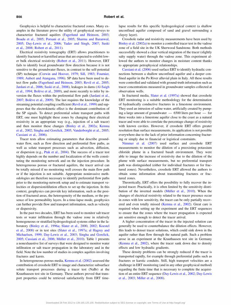
Geophysics is helpful to characterize fractured zones. Many ex-amples in the literature prove the utility of geophysical surveys tocharacterize fractured aquifers (Fagerlund and Heinson, 2003;Boadu et al., 2005; Porsani et al., 2005; Sharma and Baranwal,2005; Day-Lewis et al., 2006; Yadav and Singh, 2007; Suskiet al., 2008; Robert et al., 2011).Electrical resistivity tomography (ERT) allows practitioners to

identify fractured or karstified areas that are expected to exhibit low-er bulk electrical resistivity (Robert et al., 2011). However, ERTfails to identify local groundwater flow direction because it is notsensitive to the groundwater fluxes, in contrast to the self-potential(SP) technique (Corwin and Hoover, 1979; Sill, 1983; Fournier,1989; Aubert and Atangana, 1996). SP data have been used to de-tect flow paths (Fagerlund and Heinson, 2003; Revil et al., 2005;Jardani et al., 2006; Suski et al., 2008), leakages in dams (Al-Saighet al., 1994; Bolève et al., 2009), and more recently to infer by in-version the fluxes within the preferential flow path (Jardani et al.,2007; Bolève et al., 2009). The last requires the knowledge of thestreaming potential coupling coefficient (Revil et al., 1999) and sup-poses that the electrokinetic effect is the dominant contribution ofthe SP signals. To detect preferential solute transport paths withERT, one must highlight these zones by changing their electricalresistivity in an appropriate way (e.g., injection of a salt tracer)and then monitor these changes (Binley et al., 2002a; Kemnaet al., 2002; Singha and Gorelick, 2005; Vanderborght et al., 2005;Cassiani et al., 2006).Tracer tests allow estimating parameters that describe ground-

water flow, such as flow direction and preferential flow paths, aswell as solute transport processes such as advection, diffusion,or dispersion (e.g., Ptak et al., 2004). The success of a tracer testhighly depends on the number and localization of the wells consti-tuting the monitoring network and on the injection procedure. Inheterogeneous porous or fractured aquifers, the tracer arrival canbe totally missed if no monitoring well crosses the main flow pathor if the injection is not suitable. Appropriate noninvasive meth-odologies are therefore necessary to identify preferential flow pathsprior to the monitoring-network setup and to estimate transport ve-locities or dispersion/dilution effects to set up the injection. In thiscontext, geophysics can provide key information, such as the posi-tion of fractured areas, the heterogeneity of the medium, or the pre-sence of low permeability layers. In a time-lapse mode, geophysicscan further provide flow and transport information, such as velocityor dispersivity.In the past two decades, ERT has been used to monitor salt tracer

tests or water infiltration through the vadose zone in relativelyhomogeneous or stratified hydrogeological systems either in the la-boratory (Binley et al., 1996a; Slater et al., 2000, 2002; Koestelet al., 2008) or in test sites (Slater et al., 1997a; al Hagrey andMichaelsen, 1999; Day-Lewis et al., 2003; Singha and Gorelick,2005; Cassiani et al., 2006; Müller et al., 2010). Table 1 presentsa nonexhaustive list of surveys that were designed to monitor waterinfiltration or salt tracer propagation in the laboratory and in thefield. Note the low number of studies in complex aquifers involvingfractures and karsts.In heterogeneous porous media, Kemna et al. (2002) assessed the

contribution of crosshole ERT to image and characterize subsurfacesolute transport processes during a tracer test (NaBr) at theKrauthausen test site in Germany. These authors proved that trans-port properties could be retrieved satisfactorily from ERT time-

lapse results for this specific hydrogeological context (a shallowunconfined aquifer composed of sand and gravel surrounding aclayey layer).Crosshole radar and resistivity measurements have been used by

Binley et al. (2002a) to monitor a controlled tracer test in the vadosezone of a field site in the UK Sherwood Sandstone. Both methodssuccessfully showed a clear vertical migration of the tracer (slightlysalty supply water) through the vadose zone. This experiment al-lowed the authors to monitor changes in moisture content thanksto appropriate petrophysical relationships.Cassiani et al. (2006) used surface ERT to identify hydraulic con-

nections between a shallow unconfined aquifer and a deeper con-fined aquifer in the Po River alluvial plain in Italy. All these resultswere controlled and validated with ground-truth information such astracer concentrations measured in groundwater samples collected atobservation wells.In fractured media, Slater et al. (1997a) showed that crosshole

ERT monitoring is a suitable methodology for the determinationof hydraulically conductive fractures in a limestone environment.They used an intrusion of saline water, artificially created by pump-ing a large amount of groundwater — 6500 liters per hour — forthree weeks into a limestone aquifer close to the coast as a naturaltracer and were able to correlate the percentage change of resistivitywith known cavities. However, if crosshole ERT offers greaterresolution than surface measurements, its application is not possibleeverywhere due to the lack of prior information concerning fractur-ing or simply due to financial or logistical constraints.Nimmer et al. (2007) used surface and crosshole ERT

measurements to monitor the dilution of a preexisting potassiumchloride plume in a fractured basalt environment. They wereable to image the increase of resistivity due to the dilution of theplume with surface measurements, but no preferential transportpath was distinguished (either for individual fractures or for frac-tured zones). Nevertheless, crosshole ERT allowed the authors toobtain some information about transmitting fractures or frac-tured zones.Theoretically, ERT offers the possibility to fully recover the in-

jected tracer. Practically, it is often limited by the sensitivity distri-bution of the inverted models (Müller et al., 2010). When thechanges of electrical resistivity related to the tracer presence occurin zones with low sensitivity, the tracer can be only partially recov-ered and even totally missed (Kemna et al., 2002). Great care isrequired when setting up the experiment and the ERT sequencesto ensure that the zones where the tracer propagation is expectedare sensitive enough to detect the tracer arrival.A higher concentration of the tracer in the injected solution can

generally be used to counterbalance the dilution effects. However,this leads to denser tracer solutions, which could sink down in theaquifer rather than flow through the natural path. Such a problemarose in an experiment at the Krauthausen test site in Germany(Kemna et al., 2002), where the tracer sank down due to densityeffects and low hydraulic gradients.These density problems can be strongly reduced if the tracer is

transported rapidly, for example through preferential paths such asfractures or karstic conduits. Still, high transport velocities are achallenge in ERT monitoring (and in any other geophysical method)regarding the finite time that is necessary to complete the acquisi-tion of an entire ERT sequence (Day-Lewis et al., 2002; Day-Lewiset al., 2003; Miller et al., 2008).

B56 Robert et al.

Downloaded 28 Feb 2012 to 139.165.125.100. Redistribution subject to SEG license or copyright; see Terms of Use at http://segdl.org/

Table 1. Nonexhaustive review of the previous studies employing ERT (or DC surveys) to monitor hydrogeological processessuch as water infiltration and salt tracer propagation. The ability of ERT to image salt tracer propagation was clearlydemonstrated in the laboratory or in shallow alluvial aquifers. However, except for a few studies that investigated fracturedbedrock, we were not able to find a reference that investigated the ability of ERT to monitor a salt tracer test in complexfractured/karstified limestones or at a greater depth with only surface measurements. This study was then designed toinvestigate whether ERT and a salt tracer test could be combined to image and characterize a preferential solute transport paththrough fractured limestones. Note that MALM is “mise a la masse” and that the difference between a positive and a negativetracer is related to the effect of the tracer on the bulk electrical resistivity. A positive tracer (e.g., salty water; our case)decreases the bulk electrical resistivity, whereas a negative tracer increases it (e.g., pure water).

Geology

Saturated orunsaturated

zone Tracer Velocity (m∕day)Ratio of

conductivityDepth(m)

ERT (eventuallyDC survey)

White (1988, 1994) Coarse gravels Saturated Salt injection �260 to 700 / <10 Surface and MALM

Bevc and Morrison(1991)

Clay/silt and sand/gravel layers

Saturated Salt injection/pumpingStrong channel flowpaths

26 <40 Borehole-to-surface

Daily et al. (1992) Clay/silt and sand/gravel layers

Unsaturated Infiltration test >7.6 (vertical) — <17 Crosshole

Daily and Ramirez(1995)

Sand and clay layersUnsaturated Infiltration test “preferentialpermeability paths”

— 10 to30

Crosshole andsurface

Daily et al. (1995) Sandy silt (LAB) Saturated Salt injection — 12.5 <5 Crosshole andsurface

Osiensky andDonaldson (1995)

Sand and gravels Saturated Salt injection — 16 <10 MALM

Binley et al. (1996a,1996b)

Silty and clay loam(LAB)

Saturated Salt injection 0.084 (vertical) 2.5 <0.6 Crosshole

Ramirez et al. (1996) Sand (LAB) Saturated Salt injection — 100 <10.7 Crosshole

Slater et al. (1997a) Fractured/karstifiedlimestone

Saturated Seawater migration <220 3 to 4 8 to 28 Crosshole

Slater et al. (1997b) Chalk Unsaturated Infiltration test >11.6 (vertical) — <15.5 Crosshole

Barker and Moore(1998)

Sand and gravel Unsaturated Infiltration test �2 (vertical) — <5 Surface

Park (1998) Clay/silt and sand/gravel layers

Unsaturated Infiltration test — — <50 Surface

Slater and Sandberg(2000)

Soil overlyingfractured bedrock

Both Natural salt infiltration — / <10 Surface

Slater et al. (2000) Sand and clay layers(LAB)

Saturated Salt injection �0.7 (vertical) 1480 <3 Crosshole

Binley et al. (2002a) Sandstone Unsaturated Salt injection �0.4 (vertical) — <10 Crosshole

Binley et al. (2002b) Sandstone Unsaturated Seasonal variation �0.07 (vertical) — <10 Crosshole

Kemna et al. (2002) Clay/silt and sand/gravel layers

Saturated Salt injection �1 19 <10 Crosshole andsurface

Nimmer and Osiensky(2002a, 2002b)

Fractured basalt Partiallysaturated

Salt injection — 20 <8 Borehole-to-surfaceand MALM

Slater et al. (2002) Sand with a gravelchannel (LAB)

Saturated Salt injection �0.5 (vertical) 168 <2 Crosshole

Singha and Gorelick(2005)

Sand and gravel Saturated Salt injection 0.4 to 1.9 195 7 to 30 Crosshole

Cassiani et al. (2006) Clay/silt and sand/gravel layers

Saturated Salt injection — 5 to 10 5 to 15 Surface

Nimmer et al. (2007) Fractured basalt Saturated Salt plume dilution — 5 <10 Crosshole andsurface

Oldenborger et al.(2007)

Sand and gravels Saturated Salt injection/pumping — >50 <18 Crosshole

Koestel et al. (2008) Sandy soil (LAB) Saturated Salt injection — 5 <1.5 Crosshole

Hayley et al. (2009) Silt/clay and sand Both Salt pollution — — <10 Surface

Müller et al. (2010) Clay/silt and sand/gravel layers

Saturated Positive and negativetracer injection

�1 6 and 1∕4 <10 Crosshole andsurface

Wilkinson et al. (2010) Sand Saturated Salt injection �0.5 — <8 m Crosshole

This study Fractured/karstifiedlimestone

Saturated Salt injection >240 92 and 242 20 to30

Surface

A salt tracer test monitored with ERT B57

Downloaded 28 Feb 2012 to 139.165.125.100. Redistribution subject to SEG license or copyright; see Terms of Use at http://segdl.org/

The aim of our study was to set up a qualitative monitoring ex-periment to confirm and characterize preferential flow paths at asmall-basin scale in a fractured/karstified limestone aquifer usingsurface ERT measurements. Because previous workers focusedmainly on crosshole ERT and on shallow aquifers (Table 1), weperformed this experiment to prove the ability of surface ERT toimage a preferential solute transport path at a greater depth (20to 30 m). A previous geophysical study (Robert et al., 2011) al-lowed us to identify potential fractured zones and/or karstic con-duits in carboniferous limestones of southern Belgium and toposition wells for hydrogeological studies. We used one of thesesites to perform this experiment.We conducted a continuous natural gradient salt tracer test to

characterize a preferential flow path in terms of geometry and di-rection but also in terms of solute transport properties. In complexheterogeneous systems, such tracer tests monitored with surfaceERT constitute a real challenge because of the strong dilution ef-fects (which will reduce the “field of view” of ERT) and the hightransport velocities (for which great care on the acquisition se-quences is needed). Moreover, a good compromise between depthof investigation and resolution was needed because previous results(Robert et al., 2011) showed that the targeted fractured zone was at adepth of 20 m.The paper is organized as follows. We will present our experi-

mental site in terms of location, geology, and hydrogeology. Wewill then describe our experimental methodology, the way we

estimated the depth of investigation, the background-resistivity var-iations and the inversion algorithm. Results associated with two dif-ferent tracer injections that only differ by the salt concentration willthen be discussed. Conclusions and recommendations willfinally be presented.

EXPERIMENTAL SITE

To prove that monitoring a salt tracer test with ERT is feasible incomplex hard-rock systems, we needed to conduct the experimenton a site where preferential flow paths were identified. The Have-lange site, situated in southern Belgium (Figure 1), meets these re-quirements because fractured zones and karstic conduits werepreviously identified with ERT and SP profiles (Robert et al.,2011). Our injection well was drilled on the basis of the results ofthese geophysical profiles and this borehole crosses numerous frac-tures between 8 and 20 m below ground surface. The hydraulic con-ductivity of this well was estimated at 10−4 m∕s by a pumping test(Brouyère et al., 2009). This is only an order of magnitude becausethe drawdown during the pumping test was extremely low (0.69 mwith a pumping rate of 20 m3∕h).The Havelange site lies in a carboniferous limestone syncline

which is a part of the Dinant Synclinorium geological struc-ture (Figure 1). This synclinorium is a succession of lateTournaisian-Visean calcareous synclines and late Famenniansandstones anticlines corresponding to the main valleys andcrests, respectively. An impermeable shale layer is also situatedbetween the limestones and the sandstones. All these structuresare oriented northeast–southwest (Figure 1).The carboniferous limestones in the Havelange site are highly

fractured and karstified and create a complex groundwater flow sys-tem. These fractured zones as well as the karstic conduits can beevidenced in nearby quarries. The Havelange calcareous synclineis about 800 m wide and 6500 m long, and the difference in eleva-tion between the nearby sandstone crests and this particular lime-stone valley is about 60 m. Therefore, we included the topographyin the ERT data inversion.In the studied area, groundwater flow is controlled by two per-

pendicular hydraulic gradients (Figure 1). The first gradient, alongthe main fold axis direction (northeast–southwest), is prescribed bythe nearby Hoyoux River (Brouyère et al., 2009) and can be esti-mated at about 0.01 — that is, 1 m (elevation) per 100 m (along thetopography). As a consequence, groundwater flows toward thenortheast in the Havelange syncline. The second gradient is linkedto the flanks of the calcareous valley, with groundwater flowingfrom the flanks of the valley toward its center (Figure 1). This gra-dient is difficult to estimate given the absence of piezometers in thisarea. Nevertheless, in a nearby syncline, it ranges between 0.005and 0.02 — that is, between 0.5 and 2 m (elevation) per 100 m(along the topography), respectively.In the vicinity of the injection well, situated on the southern flank

of the syncline, both gradients play an important role but it is dif-ficult to determine in what proportions. It was however crucial toestimate the local groundwater flow direction to position our ERTprofiles correctly. The results of an SP profile (Robert et al., 2011)showed that the hydraulic gradient linked to the southern flank ofthe valley could not be neglected. By assuming that both gradientswere equal in proportions, we estimated the local groundwater flowdirection to be N15°E.

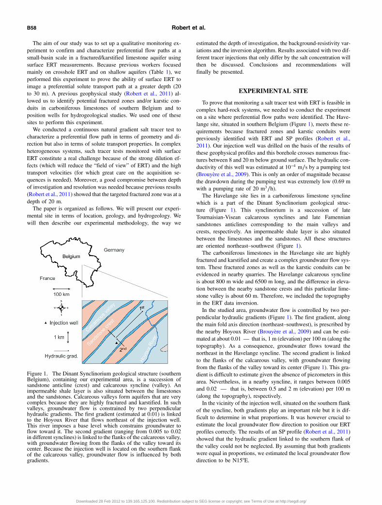
Figure 1. The Dinant Synclinorium geological structure (southernBelgium), containing our experimental area, is a succession ofsandstone anticline (crest) and calcareous syncline (valley). Animpermeable shale layer is also situated between the limestonesand the sandstones. Calcareous valleys form aquifers that are verycomplex because they are highly fractured and karstified. In suchvalleys, groundwater flow is constrained by two perpendicularhydraulic gradients. The first gradient (estimated at 0.01) is linkedto the Hoyoux River that flows northeast of the injection well.This river imposes a base level which constrains groundwater toflow toward it. The second gradient (ranging from 0.005 to 0.02in different synclines) is linked to the flanks of the calcareous valley,with groundwater flowing from the flanks of the valley toward itscenter. Because the injection well is located on the southern flankof the calcareous valley, groundwater flow is influenced by bothgradients.

B58 Robert et al.

Downloaded 28 Feb 2012 to 139.165.125.100. Redistribution subject to SEG license or copyright; see Terms of Use at http://segdl.org/

The transport velocity values in such complexly fractured andkarstified systems are extremely variable with values ranging be-tween 5 and 225 m∕hour. Results of classic tracer tests performedin some calcareous valleys of the Dinant and Namur Synclinoriumgeological structures are summarized in Brouyère et al. (2009).The injection well is equipped with a PVC casing with a diameter

of 125 × 112 mm (ext × int). Screens (with an aperture of 2 mm)begin at a depth of 16.4 m and extend to the bottom of the wellat 45 m. The diameter of the well is 250 mm. The gravel pack(4-6 mm caliber) has a radius of 62.5 mm through the entirescreened zone. We measured the water table at a depth of11.38 m and this value was constant during the entire experiment.

EXPERIMENTAL METHODOLOGY

We monitored the salt tracer propagation with two parallel ERTprofiles placed perpendicularly to the estimated local groundwaterflow direction (approximately N15°E), to cross the salt tracer pro-pagation path and better constrain it. These two transverse ERT pro-files were placed 15 m and 30 m from the injection well.We also placed a third longitudinal ERT profile (called L) in the

estimated local groundwater flow direction with the aim of obser-ving the propagation of the salt tracer in time. However, it was notaligned with the real tracer transport path (about 5 to 10° away) andno significant anomalies were observed on the results. These resultsare therefore not presented in this paper.We chose to set up the ERT profiles to have a sufficient depth of

investigation (30 m) by taking a minimum of 200 m for the length ofeach ERT profile (Table 2).

To deal with resolution problems, we used two different electrodespacings for both transverse profiles (Table 2). The nearest one(called P1) has 72 electrodes with a spacing of 3 m (213 m long),whereas the farthest one (called P2) has 48 electrodes with a spacingof 5 m (235 m long). We left the cables and the electrodes in placeduring the 3 days of the experiment.We measured every electrode location with a differential GPS

(Leica GPS1200, Leica Geosystems) to take the topography intoaccount. The vertical and horizontal accuracies are estimated tobe better than 3 cm.To establish the background when there is no injection, we col-

lected two data sets (on 15 and 16 March 2010, respectively).In this experiment, we needed to ensure that the tracer would not

sink into the well but rather flows through the fractured zone. Wetherefore placed a packer in the well at a depth of 20 m (lower limitof the fractured zone). The strong hydraulic gradients of the studiedarea result in high transport velocities that prevent the salt tracerfrom sinking once flowing in the fractured zone.We performed the tracer experiment twice (on 16 March 2010

and 17 March 2010) to demonstrate its reproducibility and to ad-dress uncertainties associated with dilution effects (by increasingthe salt concentration between both tests) and the local groundwaterflow direction (by eventually changing the location of the longitu-dinal ERT profile). The only difference between the two tests is thesalt (NaCl) concentration in the injected solution, which is 38 g∕Lfor the first test (Table 3) and 154 g∕L for the second test. Toachieve this, we used 384 kg of salt for both tests (76 kg for test1 and 308 kg for test 2).

Table 2. ERT parameters. The Rs check option allows the measurement and storage of the contact resistances.

ERT parameters Profile 1 (P1) Common to both profiles Profile 2 (P2)

Electrode array Dipole-dipole (n ≤ 6)

Electrode number 72 48

Data points 1225 629

Electrode spacing 3 m 5 m

Length of the profile 213 m 235 m

Depth of investigation (DOI) �30 m �50 m

Distance from injection well 15 m 30 m

Number of stacks 3 to 6

Quality factor 1%

Current injection time window (Ton) 1 s

Rs check For selected sequences

Reciprocal measurements For background sequences

Sequence optimization Up to 6 channels used (because n ≤ 6)

Syscal parameters Vp ¼ 800 mV − Vab max ¼ 800 V

Duration of the sequence 43 min (55 with Rs check) 20 min (26 with Rs check)

Static inversion parameters Robust data constraint and blocky inversion

Final absolute error near 2%

Time-lapse inversion parameters Robust smoothness constraint

Simultaneous inversion (data difference)

First background image as a reference

A salt tracer test monitored with ERT B59

Downloaded 28 Feb 2012 to 139.165.125.100. Redistribution subject to SEG license or copyright; see Terms of Use at http://segdl.org/

Given the expected high transport velocities, we injected the tra-cer solution during 4 hours to maintain the changes in electricalresistivity long enough to visualize the salt tracer propagation.The injection rate was limited to approximately 500 L∕h to preservethe natural hydraulic gradient of the area, as evidenced by the hy-draulic head observed in the injection well.One critical issue with fast transport processes is the finite time

that is required to complete the data collection of one entire ERTimage (e.g., Miller et al., 2008). To reduce the data acquisition time,we optimized a dipole-dipole configuration with n ≤ 6 for multi-channel acquisition (maximum 6 channels used) by sorting the se-quence in a way that no pair of potential electrodes was used after atransmitter current injection. This also allowed us to scan the sub-surface from one side of the profile to the other one. Electrical datawere acquired with an IRIS SYSCAL PRO device.Another way to reduce the data acquisition time is to reduce the

transmitter-current-injection time window. However, this could leadto poorer data quality. In this experiment, we chose a current injec-tion time window equal to 1 second with minimum three (maximumsix) stacks performed with a quality factor of 1%. These parametersresulted in a duration of about 45 minutes for P1 and 25 minutes forP2 and L. Although this parameter set is not the fastest one, webelieved that the data quality was more important than gaining extratime-lapse images, at this stage.We designed the acquisition of ERT images with the idea to move

away from the injection well during the time elapsed. A sequencewas then designed as follows. First, the longitudinal profile L (noresults are shown in this work) was collected (25 min), then P1(45 min) and finally, P2 (25 min). A complete sequence of acquisi-tion (L, P1, and P2) took approximately 1.5 hours. Data acquisitionstarted approximately 40 minutes after the beginning of the injec-tion for the first test (10 minutes for the second test).We monitored the fluid electrical conductivity (with a YSI 650

MDS multiparameter probe) throughout all the experiment in themiddle of the injection window at a depth of 18 m, to know exactlywhen the tracer injection into the aquifers was complete and there-fore when to stop measuring. We acquired seven complete se-quences of acquisition for both tests until the ratio between theelectrical conductivity measured in the well and the natural ground-water electrical conductivity was less than a tenth of its maximum.

Every measurement of electrical conductivity presented is for agroundwater temperature that was equal to 9.85°C throughoutthe experiment.The electrical conductivity of groundwater before injection was

measured in the well at about 0.52 mS∕cm, corresponding to miner-alized water (mostly calcium, magnesium, and carbonate). Theinjected solution containing the salt tracer had an electrical conduc-tivity of about 48 mS∕cm for a salt concentration of 38 g∕L (test 1),whereas it was 147 mS∕cm for 154 g∕L (test 2). The ratio of elec-trical conductivity between the injected solution and the naturalgroundwater is equal to 92 (test 1) and 282 (test 2). This correspondsto nearly two and three orders of magnitude for test 1 and test 2,respectively.Table 1 presents a comparison of our tracer test parameters with

previous studies. Here, we did not perform a complete review of theliterature but we rather wanted to highlight the lack of such studiesin complex aquifers involving fractures and karsts. Note that theratio of electrical conductivity of the injected solution between bothtests is only tripled, while the salt concentration is quadrupled. In-deed, the relationship between salt concentration and electrical con-ductivity does not remain linear at high concentration (e.g., Kemnaet al., 2002). Note also that we injected the tracer at the top of thewell and that it was already diluted before flowing into the fracturedarea. Hence, the maximum ratio measured in the well was about 80for test 1 and 150 for test 2, whereas the same ratio in the injectedsolution was 92 for test 1 and 282 for test 2.

ERROR ANALYSIS

To estimate the data noise level, we performed reciprocal mea-surements (swapping current and potential electrodes) on selectedsequences. The reciprocal error, which is the difference betweennormal and reciprocal electrical resistances, is often used as a dataquality indicator (LaBrecque et al., 1996; Slater et al., 2000; Koestelet al., 2008).When comparing normal and reciprocal measurements, it is es-

sential to collect the data sets under identical conditions. Therefore,in our experiment where high transport velocities were expected, itwas useless to collect reciprocal measurements during the entire salttracer injection. Thus, we collected reciprocal measurements onlyfor both background sequences as well as for the sequences between

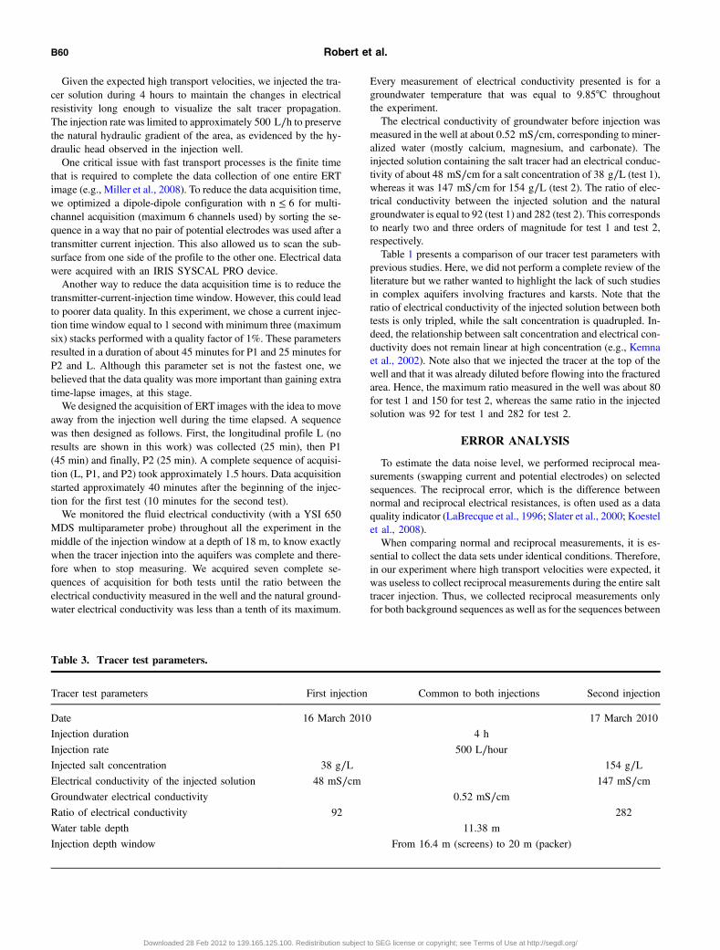
Table 3. Tracer test parameters.

Tracer test parameters First injection Common to both injections Second injection

Date 16 March 2010 17 March 2010

Injection duration 4 h

Injection rate 500 L∕hourInjected salt concentration 38 g∕L 154 g∕LElectrical conductivity of the injected solution 48 mS∕cm 147 mS∕cmGroundwater electrical conductivity 0.52 mS∕cmRatio of electrical conductivity 92 282

Water table depth 11.38 m

Injection depth window From 16.4 m (screens) to 20 m (packer)

B60 Robert et al.

Downloaded 28 Feb 2012 to 139.165.125.100. Redistribution subject to SEG license or copyright; see Terms of Use at http://segdl.org/

the first and second tests. The analysis of the reciprocal error dis-tribution shows that the average noise level varies less than 0.1%from 15 March to 17 March 2010.The acquisition of reciprocal measurements is also time-consum-

ing because a sequence needs to be collected twice. At this stage, webelieved that gaining more normal images was more useful thancollecting reciprocal measurements of every image (that are possi-bly not related to the same state of tracer arrival).Noise reduction is crucial, as the changes in the data linked to the

tracer arrival are of the same order of magnitude as the data error.Here, we were able to maintain the reciprocal error distribution be-tween −2 and 2%, except for a few outliers that were removed fromall data sets. The standard deviation of the reciprocal error distribu-tion is also lower than 0.5%. This is satisfactory given the higherpercentage change in the data linked to the tracer arrival (a fewpercentage points).

DEPTH OF INVESTIGATION

The depth of investigation is defined by the depth below whichthe electrical structures do not depend on the surface data anymore(Oldenburg and Li, 1999). Below this depth, it is assumed that elec-trical structures are linked to the initial and prior or reference modelused in the inversion process. Therefore, if changes in the electricalstructures (e.g., forced by a salt tracer test) are located below thedepth of investigation, we assume that they will not affect the sur-face data and that these changes cannot be retrieved in the time-lapse images. Thus, we decided to filter all ERT images by selectingan appropriate cutoff value for the depth-of-investigation indicator.This way, we avoid interpreting artifacts as changes in resistivityresulting from the tracer arrival.Several techniques exist to estimate the depth of investigation or

to identify possible artifacts in the electrical structures. Amongthem, the resolution (e.g., Alumbaugh and Newman, 2000; Friedel,2003; Oldenborger and Routh, 2009) or sensitivity (e.g., Nguyenet al., 2009) matrix analysis and/or the depth of investigation(DOI) index (e.g., Oldenburg and Li, 1999; Marescot et al.,2003) analysis are often used. We used the relative sensitivity ma-trix computed by the Res2Dinv software (Loke and Barker, 1996)because this parameter gives a direct indication of the sensitivity ofmeasurements subject to changes in the electrical structures.To estimate the right cutoff value for the sensitivity, we per-

formed extra tests in the Havelange site on 22 April 2010. We usedan EM39 electromagnetic induction probe (Geonics Limited) to re-cover information about the bulk electrical resistivity in the injec-tion well. Because the gravel pack (radius of 62.5 mm) only slightlyinfluences apparent electrical resistivity measurements (McNeill,1986), we assumed that the EM39 log is sufficiently representativeof the bulk electrical resistivity. We took measurements every halfmeter, starting from the bottom of the well. Because this techniquerequires PVC casing, we stopped measuring once we arrived nearthe metal casing that supports overburden (5 m from the surface).Preliminary tests conducted in February 2010 included an ERT

profile centered on the injection-well position. These tests were de-signed to compare several acquisition parameters to find the bestcompromise between good data quality and rapid acquisition.The data acquired using the same acquisition parameters as the tra-cer test parameters were inverted by using the same parameters asfor the tracer test experiment, and an ERT log was extracted at thewell’s position. We compared this ERT log with the EM39 log to

find a correct cutoff value. We believe that this methodology gives agood estimate of the depth of investigation even if ERT and EM39do not investigate the same volume of material. Often, the cutoffvalue is arbitrarily chosen (Oldenburg and Li, 1999; Marescotet al., 2003), whereas here we base our choice on the comparisonbetween two values of the resistivity obtained independently.A strong discrepancy between the ERT and EM39 logs can be

seen at a depth of 32 m (Figure 2, discrepancy C). At this depth,the relative sensitivity value is about 0.1, which is our cutoff valuefor depth of investigation. This relative sensitivity cutoff value wasapplied on the time-lapse images to avoid interpreting artifactsat depth.The depth of investigation in the central part of the images is

sufficient with 30 m for P1 and 50 m for P2. Indeed, this is10 m below the expected changes of electrical resistivity (near20 m deep) for P1 and 30 m below for P2. The electrical resistivityimages and their relative sensitivity images are presented in Figure 3for P1 and in Figure 4 for P2.

BACKGROUND-RESISTIVITY VARIATIONSAND TIME-LAPSE INVERSION

To set a cutoff value for the percentage change in resistivity thatwill separate physically based anomalies due to the tracer arrivalfrom artifacts caused by noise, two different background measure-ments were taken on 15 and 16 March 2010, just before the start ofinjection, for both profiles. These data were inverted in a time-lapse

Figure 2. Resolution indicators are essential to avoid misinterpre-tation of the inverted electrical structures or the anomalous percen-tage changes in resistivity. We estimated the relative sensitivitycutoff value by comparing an EM39 log and an ERT profile cen-tered on the injection-well position. The ERT log is extracted fromthe ERT image (dipole-dipole configuration, all acquisition and in-version parameters being the same as the profiles used to monitorthe salt tracer propagation) and compared with the EM39 log. Thefirst discrepancy between the ERT and EM39 logs (A) is situatednear the water-table depth. The second discrepancy (B) is at a depthof 25 m. The strongest discrepancy (C) is situated near a depth of30 m. Below this depth, the ERT log never corresponds with theEM39 log again, so we conclude the ERT value is erroneous.We therefore used the relative sensitivity value at 30 m as a cutoffvalue (0.1).

A salt tracer test monitored with ERT B61

Downloaded 28 Feb 2012 to 139.165.125.100. Redistribution subject to SEG license or copyright; see Terms of Use at http://segdl.org/

framework to estimate the time-lapse background-resistivity varia-tions between two images where no changes should be observed.The results of this time-lapse inversion are presented in Figure 5

in the form of a histogram of percentage changes in resistivity. Notethat we used the following convention to calculate this percentagechange

pc ¼ 100%ðρ0 − ρTÞ

ρ0(1)

The percentage change in resistivity is pc, wheras ρ0 and ρT are,respectively, the electrical resistivity of the background image andthe resistivity of the image at time T. Following this equation, adecrease in electrical resistivity, e.g., due to the salt tracer arrival,will result in an increase of the percentage change in resistivity.Figure 5 shows that almost every value of percentage change in

resistivity (for P1 and P2) is between −3 and 3%. This value can beconsidered to be the resistivity changes due to “background” noise.Because we expected positive values for the percentage change inresistivity due to the tracer arrival, we used 3% as a cutoff valueabove which time-lapse variations are significant.Figure 6 shows an example of the application of both cutoff va-

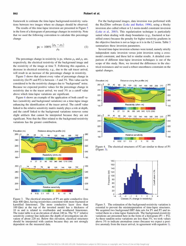
lues (sensitivity and background variations) on a time-lapse imageenhancing the identification of the tracer arrival. The cutoff valuelinked to the relative sensitivity matrix mainly plays a role at depth,and the cutoff linked to the background variations removes someslight artifacts that cannot be interpreted because they are notsignificant. Note that the filter related to the background-resistivityvariations has the greater contribution.

For the background images, data inversion was performed withthe Res2Dinv software (Loke and Barker, 1996), using a blockyinversion also called robust or L1-norm-model constraint inversion(Loke et al., 2003). This regularization technique is particularlysuited when dealing with sharp boundaries (e.g., fractured or kar-stified zones) because the penalty for higher resistivity gradients inthe objective function is not as large as it is in the L2 norm. Table 3summarizes these inversion parameters.Several time-lapse inversion schemes were tested, namely strictly

independent static inversion versus joint inversion using a cross-model constraint, and these led to similar results. A detailed com-parison of different time-lapse inversion techniques is out of thescope of this study. Here, we inverted the differences in the elec-trical resistances and we used a robust smoothness constraint on thespatial changes.

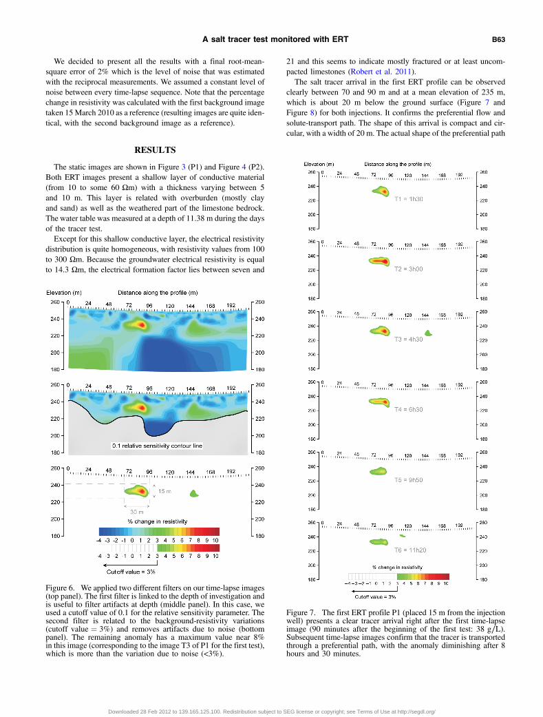
Figure 3. The electrical structures of P1 are quite conductive (lessthan 400 Ωm), having resistivities consistent with more fractured orkarstified limestones. The more conductive layer (less than100 Ωm) at the top of the inverted model has a thickness of10 m and is related to overburden and weathered limestones.The water table is at an elevation of about 240 m. The “0.1” relativesensitivity contour line indicates the depth of investigation (an ele-vation of about 220 m). Below this elevation, electrical structuresshould be interpreted with caution because they are not stronglydependent on the measured data.

Figure 4. The electrical structures of P2 are similar to those of P1(Figure 3).

Figure 5. The estimation of the background-resistivity variation isessential to prevent the misinterpretation of time-lapse structures.We acquired two background ERT data sets for P1 and P2 and in-verted them in a time-lapse framework. The background-resistivityvariations are presented here in the form of a histogram (P1þ P2).As these random noise variations are less than 3%, we took valuesabove 3% to indicate anomalous zones (because we expect a posi-tive anomaly from the tracer arrival, in agreement with equation 1).

B62 Robert et al.

Downloaded 28 Feb 2012 to 139.165.125.100. Redistribution subject to SEG license or copyright; see Terms of Use at http://segdl.org/

We decided to present all the results with a final root-mean-square error of 2% which is the level of noise that was estimatedwith the reciprocal measurements. We assumed a constant level ofnoise between every time-lapse sequence. Note that the percentagechange in resistivity was calculated with the first background imagetaken 15March 2010 as a reference (resulting images are quite iden-tical, with the second background image as a reference).

RESULTS

The static images are shown in Figure 3 (P1) and Figure 4 (P2).Both ERT images present a shallow layer of conductive material(from 10 to some 60 Ωm) with a thickness varying between 5and 10 m. This layer is related with overburden (mostly clayand sand) as well as the weathered part of the limestone bedrock.The water table was measured at a depth of 11.38 m during the daysof the tracer test.Except for this shallow conductive layer, the electrical resistivity

distribution is quite homogeneous, with resistivity values from 100to 300 Ωm. Because the groundwater electrical resistivity is equalto 14.3 Ωm, the electrical formation factor lies between seven and

21 and this seems to indicate mostly fractured or at least uncom-pacted limestones (Robert et al. 2011).The salt tracer arrival in the first ERT profile can be observed

clearly between 70 and 90 m and at a mean elevation of 235 m,which is about 20 m below the ground surface (Figure 7 andFigure 8) for both injections. It confirms the preferential flow andsolute-transport path. The shape of this arrival is compact and cir-cular, with a width of 20 m. The actual shape of the preferential path

Figure 6. We applied two different filters on our time-lapse images(top panel). The first filter is linked to the depth of investigation andis useful to filter artifacts at depth (middle panel). In this case, weused a cutoff value of 0.1 for the relative sensitivity parameter. Thesecond filter is related to the background-resistivity variations(cutoff value ¼ 3%) and removes artifacts due to noise (bottompanel). The remaining anomaly has a maximum value near 8%in this image (corresponding to the image T3 of P1 for the first test),which is more than the variation due to noise (<3%).

Figure 7. The first ERT profile P1 (placed 15 m from the injectionwell) presents a clear tracer arrival right after the first time-lapseimage (90 minutes after the beginning of the first test: 38 g∕L).Subsequent time-lapse images confirm that the tracer is transportedthrough a preferential path, with the anomaly diminishing after 8hours and 30 minutes.

A salt tracer test monitored with ERT B63

Downloaded 28 Feb 2012 to 139.165.125.100. Redistribution subject to SEG license or copyright; see Terms of Use at http://segdl.org/

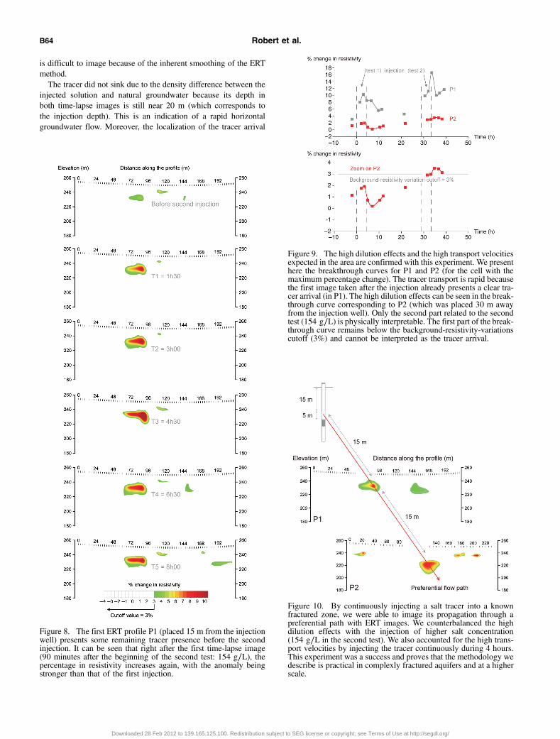
is difficult to image because of the inherent smoothing of the ERTmethod.The tracer did not sink due to the density difference between the

injected solution and natural groundwater because its depth inboth time-lapse images is still near 20 m (which corresponds tothe injection depth). This is an indication of a rapid horizontalgroundwater flow. Moreover, the localization of the tracer arrival

Figure 8. The first ERT profile P1 (placed 15 m from the injectionwell) presents some remaining tracer presence before the secondinjection. It can be seen that right after the first time-lapse image(90 minutes after the beginning of the second test: 154 g∕L), thepercentage in resistivity increases again, with the anomaly beingstronger than that of the first injection.

Figure 9. The high dilution effects and the high transport velocitiesexpected in the area are confirmed with this experiment. We presenthere the breakthrough curves for P1 and P2 (for the cell with themaximum percentage change). The tracer transport is rapid becausethe first image taken after the injection already presents a clear tra-cer arrival (in P1). The high dilution effects can be seen in the break-through curve corresponding to P2 (which was placed 30 m awayfrom the injection well). Only the second part related to the secondtest (154 g∕L) is physically interpretable. The first part of the break-through curve remains below the background-resistivity-variationscutoff (3%) and cannot be interpreted as the tracer arrival.

Figure 10. By continuously injecting a salt tracer into a knownfractured zone, we were able to image its propagation through apreferential path with ERT images. We counterbalanced the highdilution effects with the injection of higher salt concentration(154 g∕L in the second test). We also accounted for the high trans-port velocities by injecting the tracer continuously during 4 hours.This experiment was a success and proves that the methodology wedescribe is practical in complexly fractured aquifers and at a higherscale.

B64 Robert et al.

Downloaded 28 Feb 2012 to 139.165.125.100. Redistribution subject to SEG license or copyright; see Terms of Use at http://segdl.org/

is not far from the estimated local direction of flow (N5°E to N10°E,and not N15°E as previously estimated).A change of about 8% in terms of resistivity at T1, 1.5 hours after

the start of the first injection, indicates the first observation of thetracer (Figure 7). The percentage change in resistivity then increaseswithout any change in the shape of the anomaly for time T2 (3 hours,∼10%), where it reaches a plateau until time T4 (6.5 hours, ∼8%)before decreasing at times T5 (∼10 hours, ∼6%) and T6(∼11.5 hours, ∼6%) and almost totally fading (a day after stoppingthe injection). Remains of the tracer (∼4%) are nonetheless stillobserved before the start of injection of the second tracer solution(154 g∕L). Results for the second injection are similar except thatthe percentage change in resistivity is almost doubled (Figure 8).Moreover, the overall shape of the anomaly stays constant for bothinjection experiments. This is another indication that the tracer istransported through a preferential path.Results can be visualized by drawing breakthrough curves (per-

centage change in resistivity over time) for selected cells of the elec-trical resistivity model (e.g., Vanderborght et al., 2005). An examplefor the cell that presented the maximum percentage change in re-sistivity is presented for both profiles (P1 and P2) in Figure 9.The breakthrough curves for both ERT profiles clearly show that

the values of percentage change in resistivity are doubled betweenthe two tests. However, the concentration of salt in the first injection(38 g∕L) was not enough to obtain a clear arrival in the second ERTprofile (placed at 30 m from the injection well). The values are be-low the time-lapse background-resistivity variation (about 3%) andcannot be interpreted significantly as a tracer arrival (Figure 9). Thesecond injection at 154 g∕L shows an arrival (around 3.5%) of thetracer. The behavior is similar to the one for P1. Figure 10 shows theresults of one time T for both ERT profiles and proves the continuityin shape and position of the preferential flow path identified here.These breakthrough curves are also helpful to pick a first-arrival

time and to calculate its corresponding velocity. It is however dif-ficult to pick a first-arrival time here because the tracer had alreadypassed during the first image captured 90 minutes after the start ofthe injection. This means that the first tracer arrival time is clearlybelow 90 minutes. Therefore, the first-arrival velocity has a mini-mum value of 10 m∕hour and could be faster if the tracer arrivedsooner. Such transport-velocity values clearly confirm the expectedpreferential flow and solute-transport path.

CONCLUSIONS AND RECOMMENDATIONS

ERT monitoring of salt tracer tests can be useful in estimatingnew well positions, sampling rate, and tracer concentration. We

successfully highlighted a preferential flow and solute-transportpath in a very heterogeneous aquifer (a carboniferous fracturedlimestone aquifer in southern Belgium). To our knowledge, work-ing at this small-basin scale is quite rare although very importantbecause hydrogeologists can directly use the information obtainedin groundwater flow and solute transport modeling.Over a period of 4 hours, we continuously injected a salt tracer in

a previously identified fracture zone, and we monitored its propa-gation with two transverse ERT profiles. Two different salt solutions(38 and 154 g∕L) were injected and this allowed us to image thetracer arrival despite the strong dilution effects and the inherentsmoothing of ERT.In terms of geophysical imaging, we tested different electrode

spacing (3 m on the profile closest to the injection well and 5 mon the more distant profile) to deal with the resolution and the depthof investigation of our resulting images. The analysis of the relativesensitivity matrix associated with an EM39 log helped us to esti-mate the depth of investigation of both profiles (30 and 50 mfor the proximal and distal profiles, respectively). Two backgroundprofiles were taken to estimate the resistivity variations due to back-ground noise, which helped us to discriminate real tracer arrivalfrom noise artifacts.ERT images allowed us to characterize the tracer arrival in terms

of width, depth and concentration by monitoring the percentagechange in resistivity for both profiles. Some resistivity breakthroughcurves were also drawn to estimate the first-arrival time and the cor-responding velocity. This allowed us to confirm the expected hightransport velocities and the strong dilution effects but also to obtainsome information that could be crucial to set up a classic tracer test.This study proved that ERT can be used to qualitatively monitor

very rapid solute transport (>10 m∕hour) when the data acquisitionprocedure is well defined. Given the results of our study, somepoints could be improved in future work. First, the longitudinal pro-file did not give results. Therefore, we believe that gaining moretime-lapse images for the transverse profiles would have been moreinstructive and less risky. This way, we could have had a better es-timate of the first-arrival time.We used a transmitter-current-injection time window of 1 second

to obtain a good data quality. A refined breakthrough curve could beobtained by using half a second for this time window without addingtoo much noise in the data. Decreasing the number of stacks from 3–6to 2–3 will also allow more frequent sampling of the ERT image andhence a better temporal resolution of the tracer recovery.Finally, we injected the salt tracer solution at the top of the well.

As a consequence, the tracer was already (strongly) diluted beforeflowing through the fractured zone. We therefore recommend

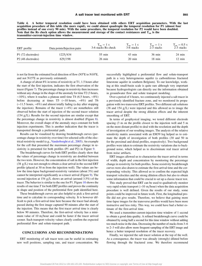
Table 4. A better temporal resolution could have been obtained with others ERT acquisition parameters. With the lastacquisition procedure of this table (the more rapid), we could almost quadruple the temporal resolution for P1 (almost fourprofiles instead of one every 90 min). With the same procedure, the temporal resolution for P2 would have been doubled.Note that the Rs check option allows the measurement and storage of the contact resistances and Ton is thetransmitter-current-injection time window.

ERT profile Data points/Injection pairsTon ¼ 1 s

3-6 stacks Rs checkTon ¼ 1 s3-6 stacks

Ton ¼ 1 s2-3 stacks

Ton ¼ 0.5 s2-3 stacks

P1 (72 electrodes) 1225∕434 55 min 43 min 36 min 24 min

P2 (48 electrodes) 629∕198 26 min 20 min 18 min 12 min

A salt tracer test monitored with ERT B65

Downloaded 28 Feb 2012 to 139.165.125.100. Redistribution subject to SEG license or copyright; see Terms of Use at http://segdl.org/

injecting the tracer at the depth of interest (in our case, the frac-tured zone).With all these changes in the acquisition procedure, we could

have obtained higher resistivity changes and almost have quad-rupled the temporal resolution for P1. Table 4 presents the acquisi-tion time of both ERT profiles with regard to differentparameters sets.Further developments of this work will be to model groundwater

flow and solute transport in the calcareous syncline structure. To doso, further geophysical and hydrogeological investigations as wellas new boreholes are necessary to fully conceptualize this aquifer.For this reason, self-potential and ERT profiles are currently beingconducted along with hydrogeological investigations to acquire in-formation for the groundwater flow model conceptualization.

REFERENCES

al Hagrey, S. A., and J. Michaelsen, 1999, Resistivity and percolation studyof preferential flow in vadose zone at Bokhorst, Germany: Geophysics,64, 746–753, doi: 10.1190/1.1444584.

Al-Saigh, N. H., Z. S. Mohammed, and M. S. Dahham, 1994, Detection ofwater leakage from dams by self-potential method: Engineering Geology,37, 115–121.

Alumbaugh, D. L., and G. A. Newman, 2000, Image appraisal for 2-D and3-D electromagnetic inversion: Geophysics, 65, 1455–1467.

Aubert, M., and Q. Y. Atangana, 1996, Self-potential method in hydrogeo-logical exploration of volcanic areas: Ground Water, 34, 1010–1016.

Barker, R., and J. Moore, 1998, The application of time-lapse electrical to-mography in groundwater studies: The Leading Edge, 17, 1454–1458.

Berkowitz, B., 2002, Characterizing flow and transport in fractured geolo-gical media: A review: Advances in Water Resources, 25, 861–884.

Bevc, D., and H. F. Morrison, 1991, Borehole-to-surface electrical resistivitymonitoring of a salt water injection experiment: Geophysics, 56, 769–777.

Binley, A., G. Cassiani, R. Middleton, and P. Winship, 2002a, Vadose zoneflow model parameterisation using cross-borehole radar and resistivityimaging: Journal of Hydrology, 267, 147–159.

Binley, A., S. Henry-Poulter, and B. Shaw, 1996a, Examination of solutetransport in an undisturbed soil column using electrical resistance tomo-graphy: Water Resources Research, 32, 763–769.

Binley, A., B. Shaw, and S. Henry-Poulter, 1996b, Flow pathways in porousmedia: Electrical resistance tomography and dye staining image verifica-tion: Measurement Science and Technology, 7, 384–390.

Binley, A., P. Winship, L. J. West, M. Pokar, and R. Middleton, 2002b,Seasonal variation of moisture content in unsaturated sandstone inferredfrom borehole radar and resistivity profiles: Journal of Hydrology, 267,160–172.

Boadu, F. K., J. Gyamfi, and E. Owusu, 2005, Determining subsurface frac-ture characteristics from azimuthal resistivity surveys: A case study atNsawam, Ghana: Geophysics, 70, no. 5, B35–B42.

Bolève, A., A. Revil, F. Janod, J. L. Mattiuzzo, and J. J. Fry, 2009, Prefer-ential fluid flow pathways in embankment dams imaged by self-potentialtomography: Near Surface Geophysics, 7, 447–462.

Brouyère, S., J. Gesels, P. Goderniaux, P. Jamin, T. Robert, L. Thomas,A. Dassargues, J. Bastien, F. Vanwittenberge, A. Rorive, F. Dossin,J.-L. Lacour, D. Le Madec, P. Nogarède, and V. Hallet, 2009, Caractér-isation hydrogéologique et support à la mise en œuvre de la DirectiveEuropéenne 2000/60 sur les masses d’eau souterraine en Région Wal-lonne (Projet Synclin’EAU): Délivrable — D.3.12 — Rapport surla caracterisation hydraulique des aquifères et l'estimation des ressourcesen eaux souterraines — Partie RWM021: Convention RW et SPGE-Aquapole.

Cassiani, G., V. Bruno, A. Villa, N. Fusi, and A. M. Binley, 2006, A salinetracer test monitored via time-lapse surface electrical resistivity tomogra-phy: Journal of Applied Geophysics, 59, 244–259.

Corwin, R. F., and D. B. Hoover, 1979, The self-potential method in geother-mal exploration: Geophysics, 44, 226–245.

Daily, W., and A. Ramirez, 1995, Electrical resistance tomography duringin-situ trichloroethylene remediation at the Savannah River site: Journalof Applied Geophysics, 33, 239–249.

Daily, W., A. Ramirez, D. LaBrecque, and W. Barber, 1995, Electrical re-sistance tomography experiments at the Oregon Graduate Institute: Jour-nal of Applied Geophysics, 33, 227–237.

Daily, W., A. Ramirez, D. LaBrecque, and J. Nitao, 1992, Electrical resis-tivity tomography of vadose water movement: Water Resources Research,28, 1429–1442.

Day-Lewis, F., J. Lane, and S. Gorelick, 2006, Combined interpretationof radar, hydraulic, and tracer data from a fractured-rock aquifernear Mirror Lake, New Hampshire, USA: Hydrogeology Journal, 14,1–14.

Day-Lewis, F. D., J. M. Harris, and S. M. Gorelick, 2002, Time-lapse in-version of crosswell radar data: Geophysics, 67, 1740–1752.

Day-Lewis, F. D., J. W. Lane, J. M. Harris, and S. M. Gorelick, 2003, Time-lapse imaging of saline-tracer transport in fractured rock using difference-attenuation radar tomography: Water Resources Research, 39, 1290, doi:10.1029/2002WR001722.

Fagerlund, F., and G. Heinson, 2003, Detecting subsurface groundwaterflow in fractured rock using self-potential (SP) methods: EnvironmentalGeology, 43, 782–794.

Fetter, C. W., 2001, Applied hydrogeology (4th ed.): Prentice-Hall.Fournier, C., 1989, Spontaneous potentials and resistivity surveys applied to

hydrogeology in a volcanic area: Case history of the Chaîne des Puys(Puy-de-Dôme, France): Geophysical Prospecting, 37, 647–668.

Friedel, S., 2003, Resolution, stability and efficiency of resistivity tomogra-phy estimated from a generalized inverse approach: Geophysical JournalInternational, 153, 305–316.

Hao, Y., T.-C. J. Yeh, J. Xiang, W. A. Illman, K. Ando, K.-C. Hsu, and C.-H.Lee, 2008, Hydraulic tomography for detecting fracture zone connectiv-ity: Ground Water, 46, 183–192.

Hayley, K., L. R. Bentley, and M. Gharibi, 2009, Time-lapse electricalresistivity monitoring of salt-affected soil and groundwater: WaterResources Research, 45, W07425, doi: 10.1029/2008wr007616.

Illman, W. A., A. J. Craig, and X. Liu, 2008, Practical issues in imaginghydraulic conductivity through hydraulic tomography: Ground Water,46, 120–132.

Illman, W. A., and D. M. Tartakovsky, 2006, Asymptotic analysisof cross-hole hydraulic tests in fractured granite: Ground Water, 44,555–563.

Jardani, A., J.-P. Dupont, and A. Revil, 2006, Self-potential signalsassociated with preferential groundwater flow pathways in sinkholes:Journal of Geophysical Research, 111, B09204, doi: 10.1029/2005JB004231.

Jardani, A., A. Revil, A. Bolève, A. Crespy, J.-P. Dupont, W. Barrash, and B.Malama, 2007, Tomography of the Darcy velocity from self-potentialmeasurements: Geophysical Research Letters, 34, L24403, doi: 10.1029/2007GL031907.

Kemna, A., J. Vanderborght, B. Kulessa, and H. Vereecken, 2002, Imagingand characterisation of subsurface solute transport using electrical resis-tivity tomography (ERT) and equivalent transport models: Journal of Hy-drology, 267, 125–146.

Koestel, J., A. Kemna, M. Javaux, A. Binley, and H. Vereecken, 2008, Quan-titative imaging of solute transport in an unsaturated and undisturbed soilmonolith with 3D ERT and TDR: Water Resources Research, 44,W12411, doi: 10.1029/2007WR006755.

LaBrecque, D. J., M. Miletto, W. Daily, A. Ramirez, and E. Owen, 1996,The effects of noise on Occam’s inversion of resistivity tomography data:Geophysics, 61, 538–548.

Liu, S., T.-C. J. Yeh, and R. Gardiner, 2002, Effectiveness of hydraulic to-mography: Sandbox experiments: Water Resources Research, 38, 1034,doi: 10.1029/2001WR000338.

Loke, M. H., I. Acworth, and T. Dahlin, 2003, A comparison of smooth andblocky inversion methods in 2D electrical imaging surveys: ExplorationGeophysics, 34, 182–187.

Loke, M. H., and R. D. Barker, 1996, Rapid least-squares inversion of ap-parent resistivity pseudosections by a quasi-Newton method: GeophysicalProspecting, 44, 131–152.

Marescot, L., M. H. Loke, D. Chapellier, R. Delaloye, C. Lambiel, and E.Reynard, 2003, Assessing reliability of 2D resistivity imaging in moun-tain permafrost studies using the depth of investigation index method:Near Surface Geophysics, 1, 57–67.

McNeill, J. D., 1986, Geonics EM39 borehole conductivity meter— Theoryof operation: Geonics Limited technical note TN-20.

Miller, C. R., P. S. Routh, T. R. Brosten, and J. P. McNamara, 2008,Application of time-lapse ERT imaging to watershed characterization:Geophysics, 73, no. 3, G7–G17.

Müller, K., J. Vanderborght, A. Englert, A. Kemna, J. A. Huisman, J. Rings,and H. Vereecken, 2010, Imaging and characterization of solute transportduring two tracer tests in a shallow aquifer using electrical resistivity to-mography and multilevel groundwater samplers: Water Resources Re-search, 46, W03502, doi: 10.1029/2008WR007595.

Nguyen, F., A. Kemna, A. Antonsson, P. Engesgaard, O. Kuras, R. Ogilvy, J.Gisbert, S. Jorreto, and A. Pulido-Bosch, 2009, Characterization of sea-water intrusion using 2D electrical imaging: Near Surface Geophysics, 7,377–390.

Nimmer, R. E., and J. L. Osiensky, 2002a, Using mise-a-la-masse to deline-ate the migration of a conductive tracer in partially saturated basalt: En-vironmental Geosciences, 9, 81–87, doi: 10.1046/j.1526-0984.2002.92005.x.

B66 Robert et al.

Downloaded 28 Feb 2012 to 139.165.125.100. Redistribution subject to SEG license or copyright; see Terms of Use at http://segdl.org/

Nimmer, R. E., and J. L. Osiensky, 2002b, Direct current and self-potentialmonitoring of an evolving plume in partially saturated fractured rock:Journal of Hydrology, 267, 258–272.

Nimmer, R. E., J. L. Osiensky, A. M. Binley, K. F. Sprenke, and B. C.Williams, 2007, Electrical resistivity imaging of conductive plume dilu-tion in fractured rock: Hydrogeology Journal, 15, 877–890.

Oldenborger, G. A., M. D. Knoll, P. S. Routh, and D. J. LaBrecque, 2007,Time-lapse ERT monitoring of an injection/withdrawal experiment in ashallow unconfined aquifer: Geophysics, 72, F177–F187.

Oldenborger, G. A., and P. S. Routh, 2009, The point-spread function mea-sure of resolution for the 3-D electrical resistivity experiment: Geophy-sical Journal International, 176, 405–414.

Oldenburg, D. W., and Y. Li, 1999, Estimating depth of investigation in DCresistivity and IP surveys: Geophysics, 64, 403–416.

Osiensky, J. L., and P. R. Donaldson, 1995, Electrical flow through an aqui-fer for contaminant source leak detection and delineation of plume evolu-tion: Journal of Hydrology, 169, 243–263.

Park, S., 1998, Fluid migration in the vadose zone from 3-D inversion ofresistivity monitoring data: Geophysics, 63, 41–51.

Porsani, J. L., V. R. Elis, and F. Y. Hiodo, 2005, Geophysical investigationsfor the characterization of fractured rock aquifers in Itu, SE Brazil: Journalof Applied Geophysics, 57, 119–128.

Post, V. E. A., 2005, Fresh and saline groundwater interaction in coastalaquifers: Is our technology ready for the problems ahead?: HydrogeologyJournal, 13, 120–123.

Ptak, T., M. Piepenbrink, and E. Martac, 2004, Tracer tests for the investiga-tion of heterogeneous porous media and stochastic modelling of flow andtransport — A review of some recent developments: Journal of Hydrol-ogy, 294, 122–163.

Ramirez, A., W. Daily, A. Binley, D. J. LaBrecque, and D. Roelant, 1996,Detection of leaks in underground storage tanks using electrical resistancetomography methods: Journal of Environmental and EngineeringGeophysics, 1, 189–203.

Revil, A., L. Cary, Q. Fan, A. Finizola, and F. Trolard, 2005, Self-potentialsignals associated with preferential ground water flow pathways in a bur-ied paleo-channel: Geophysical Research Letters, 32, L07401, doi: 10.1029/2004GL022124.

Revil, A., P. A. Pezard, and P. W. J. Glover, 1999, Streaming potential inporous media 1. Theory of the zeta potential: Journal of Geophysical Re-search, 104, B9, doi: 10.1029/1999JB900089.

Robert, T., A. Dassargues, S. Brouyère, O. Kaufmann, V. Hallet, and F.Nguyen, 2011, Assessing the contribution of electrical resistivity tomo-graphy (ERT) and self-potential (SP) methods for a water well drillingprogram in fractured/karstified limestones: Journal of Applied Geophy-sics, 75, 42–53.

Sharma, S. P., and V. C. Baranwal, 2005, Delineation of groundwater-bearing fracture zones in a hard rock area integrating very low frequencyelectromagnetic and resistivity data: Journal of Applied Geophysics, 57,155–166.

Sill, W. R., 1983, Self-potential modeling from primary flows: Geophysics,48, 76–86.

Singha, K., and S. M. Gorelick, 2005, Saline tracer visualized with three-dimensional electrical resistivity tomography: Field-scale spatial moment

analysis: Water Resources Research, 41, W05023, doi: 10.1029/2004WR003460.

Slater, L., A. Binley, R. Versteeg, G. Cassiani, R. Birken, and S. Sandberg,2002, A 3D ERT study of solute transport in a large experimental tank:Journal of Applied Geophysics, 49, 211–229.

Slater, L., A. M. Binley, W. Daily, and R. Johnson, 2000, Cross-hole elec-trical imaging of a controlled saline tracer injection: Journal of AppliedGeophysics, 44, 85–102.

Slater, L., M. D. Zaidman, A. M. Binley, and L. J. West, 1997b, Electricalimaging of saline tracer migration for the investigation of unsaturatedzone transport processes: Hydrology and Earth System Sciences, 1,291–302.

Slater, L. D., A. Binley, and D. Brown, 1997a, Electrical imaging of fracturesusing ground-water salinity change: Ground Water, 35, 436–442.

Slater, L. D., and S. K. Sandberg, 2000, Resistivity and induced polarizationmonitoring of salt transport under natural hydraulic gradients: Geophy-sics, 65, 408–420.

Suski, B., F. Ladner, L. Baron, F. D. Vuataz, F. Philippossian, and K.Holliger, 2008, Detection and characterization of hydraulically active frac-tures in a carbonate aquifer: Results from self-potential, temperature andfluid electrical conductivity logging in the Combioula hydrothermal systemin the southwestern Swiss Alps: Hydrogeology Journal, 16, 1319–1328.

Vanderborght, J., A. Kemna, H. Hardelauf, and H. Vereecken, 2005, Poten-tial of electrical resistivity tomography to infer aquifer transport charac-teristics from tracer studies: A synthetic case study: Water ResourcesResearch, 41, W06013, doi: 10.1029/2004WR003774.

White, P. A., 1988, Measurement of ground-water parameters using salt-water injection and surface resistivity: Ground Water, 26, 179–186.

White, P. A., 1994, Electrode arrays for measuring groundwater flow direc-tion and velocity: Geophysics, 59, 192–201.

Wilkinson, P. B., P. I. Meldrum, O. Kuras, J. E. Chambers, S. J. Holyoake,and R. D. Ogilvy, 2010, High-resolution electrical resistivity tomographymonitoring of a tracer test in a confined aquifer: Journal of Applied Geo-physics, 70, 268–276.

Wu, C.-M., T.-C. J. Yeh, J. Zhu, T. H. Lee, N.-S. Hsu, C.-H. Chen, and A. F.Sancho, 2005, Traditional analysis of aquifer tests: Comparing apples tooranges?: Water Resources Research, 41, W09402, doi: 10.1029/2004WR003717.

Yadav, G. S., and S. K. Singh, 2007, Integrated resistivity surveys for de-lineation of fractures for ground water exploration in hard rock areas:Journal of Applied Geophysics, 62, 301–312.

Yeh, T.-C. J., and S. Liu, 2000, Hydraulic tomography: Development of anew aquifer test method: Water Resources Research, 36, 2095–2105, doi:10.1029/2000WR900114.

Yin, D., and W. A. Illman, 2009, Hydraulic tomography using temporal mo-ments of drawdown recovery data: A laboratory sandbox study: WaterResources Research, 45, W01502, doi: 10.1029/2007WR006623.

Zhu, J., and T.-C. J. Yeh, 2005, Characterization of aquifer heterogeneityusing transient hydraulic tomography: Water Resources Research, 41,W07028, doi: 10.1029/2004WR003790.

Zhu, J., and T.-C. J. Yeh, 2006, Analysis of hydraulic tomography usingtemporal moments of drawdown recovery data: Water Resources Re-search, 42, W02403, doi: 10.1029/2005WR004309.

A salt tracer test monitored with ERT B67

Downloaded 28 Feb 2012 to 139.165.125.100. Redistribution subject to SEG license or copyright; see Terms of Use at http://segdl.org/