Embed Size (px)
Citation preview

1
A Review of the Analytical Methods used for Seaplanes Performance Prediction
Jafar Masri¹, Laurent Dala² and Benoit Huard³
¹PhD Research student, Department of Mechanical and Construction Engineering Northumbria University at Newcastle
Newcastle upon Tyne, United Kingdom *Corresponding Author
²Professor of Mechanical Engineering, Head of Department of Mechanical and Construction Engineering
Northumbria University at Newcastle Newcastle upon Tyne, United Kingdom
³Senior Lecturer, Department of Mathematics, Physics and Electrical Engineering Northumbria University at Newcastle
Newcastle upon Tyne, United Kingdom [email protected]
Abstract: the present study aims to review the conventional analytical methods used to predict the performance of seaplanes and define the weaknesses in each method along with its applicability range. The study also addresses the main issues in the design of seaplanes and provides a brief description of their motion characteristics. The heave and pitch equations of seaplane motion are also discussed and the procedure of obtaining their solution is explained. After that, the results obtained from the most common two approaches are presented. The results show that the methods have many limitations and only applicable under certain conditions. There is insufficient work to define the motion of seaplanes in the ground effect region where the craft experiences nonlinear effects. As a result, no method is optimal for all speed regimes of seaplanes. Not only that, but also most of the methods do not study the stability of seaplanes which is a major issue in the design stage. Nevertheless, no method takes in consideration the nonlinear effects of motion of seaplanes in heave and pitch axes.
Keywords: Seaplanes, Analytical, Prediction, Planing, Ekranoplan, Ground effect, Porpoising.
Nomenclature:
𝐴𝐴 Aspect ratio = 𝑏𝑏²𝑆𝑆
𝑏𝑏 Seaplane beam (m) 𝐶𝐶𝑓𝑓 Friction-drag coefficient 𝐶𝐶𝑝𝑝 Centre of dynamic pressure (m)
𝐶𝐶𝑣𝑣 Speed coefficient = 𝑉𝑉�𝑔𝑔𝑏𝑏

2
𝐶𝐶𝐿𝐿𝐿𝐿 Lift coefficient, dead-rise surface 𝐶𝐶𝐿𝐿𝐿𝐿 Lift coefficient, zero dead-rise 𝐷𝐷𝑓𝑓 Fluid friction drag (N) 𝐹𝐹3 Amplitude of the exciting force (heave) 𝐹𝐹5 Amplitude of the exciting moment (pitch)
𝐹𝐹𝑛𝑛 Froude Number = 𝑉𝑉�𝑔𝑔𝑏𝑏
𝐹𝐹𝑛𝑛∇ Volumetric Froude Number = 𝑉𝑉
�𝑔𝑔 √∇3
𝑔𝑔 Acceleration of gravity (m/s²) 𝐼𝐼55 Mass moment of inertia (kg.m²) 𝐿𝐿𝑐𝑐 Chine length (m) 𝐿𝐿𝑘𝑘 Keel length (m) 𝐿𝐿𝑚𝑚 Mean wetted length (m) 𝐿𝐿𝑤𝑤 Wetted length (m) M Moment (N.m) 𝑃𝑃𝐿𝐿 Pressure behind the stagnation point (Pa) 𝑃𝑃𝑚𝑚𝑚𝑚𝑚𝑚 Maximum pressure at stagnation point (Pa) 𝑃𝑃𝑇𝑇 Pressure at the transom (Pa) 𝑞𝑞 Pressure along the keel line (Pa) 𝑅𝑅𝑒𝑒 Reynold’s number = 𝑉𝑉𝑚𝑚𝜆𝜆𝑏𝑏
𝑣𝑣
𝑆𝑆 Wetted surface area (m²) t Time (s) 𝑉𝑉 Velocity (m/s) 𝑉𝑉𝑚𝑚 Mean velocity (m/s) ∆ or m Seaplane mass (kg) ∇ Static volume of displacement (m³) 𝑣𝑣 Kinematic viscosity of fluid (m²/s) 𝜌𝜌 Density of fluid (kg/m³) ∅ Roll angle (deg) 𝛽𝛽 Dead-rise angle (deg) 𝜏𝜏 Trim angle (deg) 𝜆𝜆 Wetted length-beam ratio 𝜆𝜆𝑦𝑦 Dimensionless distance between stagnation point and transom 𝜀𝜀 Inclination of thrust line relative to keel line (deg) ƞ Displacement coordinate vector ƞ̇ Velocity coordinate vector ƞ̈ Acceleration coordinate vector 𝜔𝜔 Circular frequency of the encounter (rad/sec)

3
Introduction:
Aviation business expects a major increase in global air traffic, while the aviation industry is under pressure to deteriorate noise and emissions. In fact, the rising concerns about noise and air pollution in the areas close to large airports are affecting the capacity and expansion of the airports. One of the potential solutions for this issue is to build airports away from populated areas in offshore locations which means moving take-off and landing paths over water. However, the cost of land reclamation and the need for new terminal buildings and pathways to be constructed is very expensive.
A substantial alternative that would abolish the need for such expensive infrastructure expenditure would be the use of waterborne aircraft. Since the beginning of the nineteenth century, the concept of waterborne ground effect aircraft (also known as Wing-In-Ground “WIG” Craft, Ekranoplan, Seaplane or Ground Effect Vehicle “GEV”) has been widely investigated due to its ability to cover a wide range of applications as well as its ability to combine between the characteristics of aircrafts and marine crafts. Moreover, as almost 71% of the earth’s surface is water, the waterborne aircraft could provide access to almost every part of the world.
According to Rozhdestvensky (2006), the WIG craft is a heavy vehicle with an engine that is designed to fly close ground or water surfaces for efficient utilization of the Ground Effect. The latter also defined the Ground Effect “GE” as an increase of the lift-to-drag ratio of a lifting surface at small distances from ground or water surfaces [1].
Seaplanes have similar performance characteristics as planing hulls as they are both designed to glide on top of water surfaces and take advantage of the positive dynamic lift produced by their motion. This was supported by Baird (1998) who claims that high speed vessels including all monohulls, catamarans and trimarans having speeds greater than 16 m/s [2]. Therefore, the appropriate hydrodynamic stability prediction is the key to a successful seaplane design.
Planing hulls have a unique instability phenomenon called porpoising which, according to Faltinsen (2005), can be defined as a periodic, bounded vertical motion that a craft might show at certain speeds [3]. This phenomenon can be seen as an oscillatory motion in the heave and pitch axes and can cause severe damage to the structure of the craft. In some cases, if the hull is leaving water and returning at negative trim angle, the craft will submarine. It is therefore very important to predict the behaviour of the seaplane in the design stage [4].
The purpose of this paper is to advance the understanding of the analytical methods used to predict the performance of seaplanes. In addition, the paper will identify the weaknesses in the current methods and discuss how the analytical approach can be extended. The first section of the paper will illustrate the seaplane motion characteristics. In the second section, the analytical methods available in the literature will be briefly discussed in which the advantages and disadvantages of each of them will be stated. After that, the heave and pitch

4
equations of seaplane motion will be presented along with a proposed solution. Lastly, the results obtained from different analytical methods will be compared and conclusion drawn.
Seaplane Motion Characteristics:
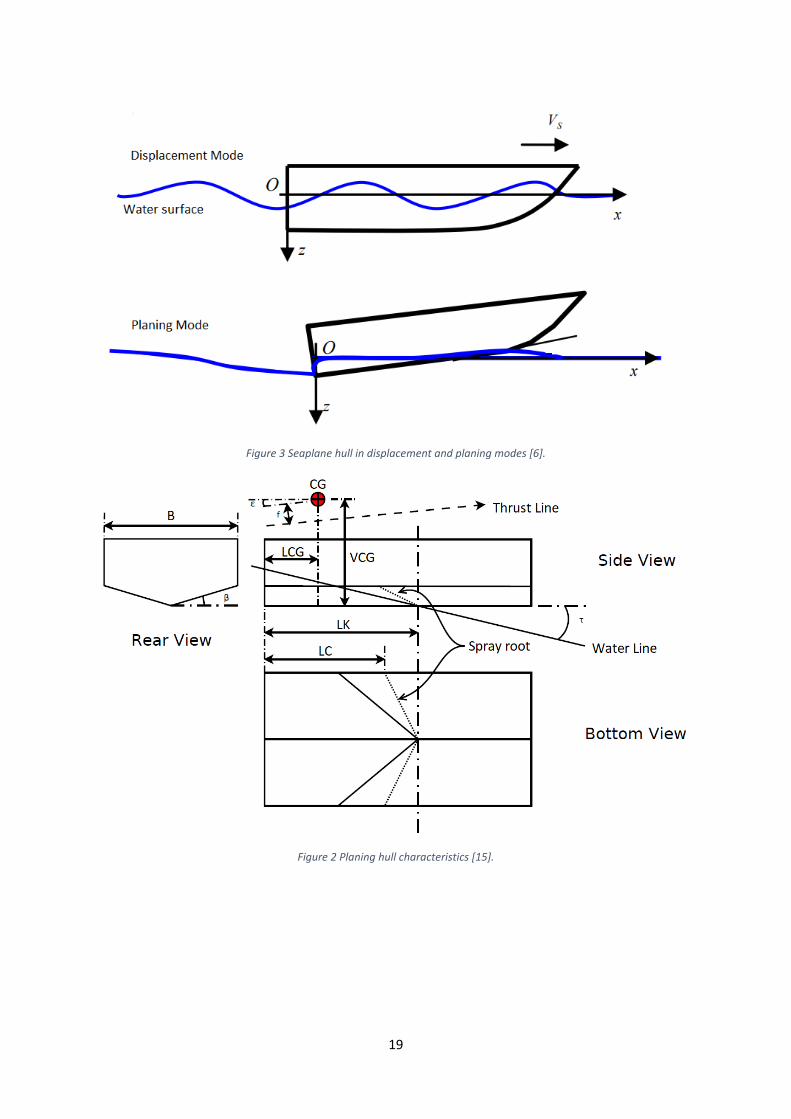
The motion of seaplanes is distinguished by many unique characteristics that exist because seaplanes operate in two media, air and water. When the seaplane leaves the surface of water, it will encounter aerodynamic forces and will have similar operational characteristics as other fixed wing airplanes. However, the motion of seaplanes on water introduces additional complications. As explained in Fig.1, the seaplane goes through a transition process from a steady state mode in which the plane is under static buoyancy (the displacement range) to a dynamic planing mode (the planing range). The seaplane must be designed to accomplish this transition smoothly and successfully between the three basic regimes which are waterborne buoyancy, waterborne planing and airborne flight.
The motion of seaplanes can be classified according to Froude number (𝐹𝐹𝑛𝑛) as follows:
• 𝐹𝐹𝑛𝑛 > 0.4: This is the displacement range. The seaplane is moving through water by pushing the water aside. In this range, there are two types of pressure forces acting on a seaplane, the hydrostatic force (buoyancy force) and the hydrodynamic force. However, the hydrostatic force (restoring force) is dominant in this region relative to the hydrodynamic forces (added mass and damping forces). According to Archimedes principle, the hydrostatic force acting on a body that is fully or partially submerged in water equals the weight of the water that the body displaces. This hydrostatic force is always in the upward direction and passes through the centre of mass of the seaplane. The seaplane must be capable of withstanding moments introduced by the action of wind and wave while travelling in this speed range [5].
• 0.4 < 𝐹𝐹𝑛𝑛 < 1.0: In this speed range the seaplane enters the planing mode (also known as semi-planing or semi-displacement mode). As the speed increases, the weight of the seaplane becomes mainly supported by hydrodynamic forces while the hydrostatic force becomes less dominant. Each of the forces has a different centre of pressure. Nevertheless, aerodynamic effects starts to play a role in lifting the seaplane off water in this region. The main challenges in the design of seaplanes are in this speed range. The seaplane must be capable of accelerating to take-off while keeping stability about all axes of motion. Also, as the seaplane accelerates from zero velocity, there is some speed at which the water resistance becomes maximum. This point is known as “hump speed point”. It is the point where the lift force shifts from being predominantly buoyant to being dynamic (hydrostatic to hydrodynamic). If the seaplane is not very well designed to over-take this issue, it will not be able to take-off [5].
• 𝐹𝐹𝑛𝑛 > 1.0: This is the fully planing range where the weight of the seaplane is mainly supported by aerodynamic forces. The seaplane has the same performance
5
characteristics as a normal airplane in this range. The three operating ranges of seaplanes are shown in Fig.2 [5].
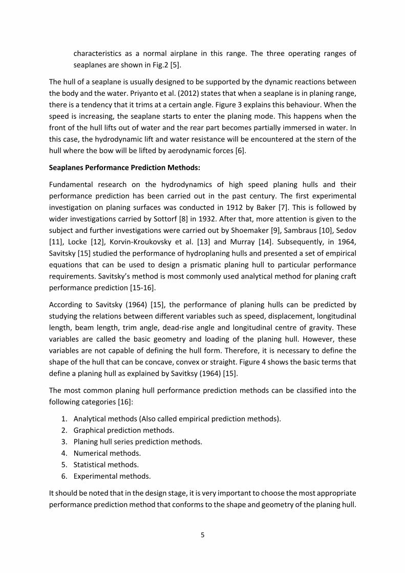
The hull of a seaplane is usually designed to be supported by the dynamic reactions between the body and the water. Priyanto et al. (2012) states that when a seaplane is in planing range, there is a tendency that it trims at a certain angle. Figure 3 explains this behaviour. When the speed is increasing, the seaplane starts to enter the planing mode. This happens when the front of the hull lifts out of water and the rear part becomes partially immersed in water. In this case, the hydrodynamic lift and water resistance will be encountered at the stern of the hull where the bow will be lifted by aerodynamic forces [6].
Seaplanes Performance Prediction Methods:
Fundamental research on the hydrodynamics of high speed planing hulls and their performance prediction has been carried out in the past century. The first experimental investigation on planing surfaces was conducted in 1912 by Baker [7]. This is followed by wider investigations carried by Sottorf [8] in 1932. After that, more attention is given to the subject and further investigations were carried out by Shoemaker [9], Sambraus [10], Sedov [11], Locke [12], Korvin-Kroukovsky et al. [13] and Murray [14]. Subsequently, in 1964, Savitsky [15] studied the performance of hydroplaning hulls and presented a set of empirical equations that can be used to design a prismatic planing hull to particular performance requirements. Savitsky’s method is most commonly used analytical method for planing craft performance prediction [15-16].
According to Savitsky (1964) [15], the performance of planing hulls can be predicted by studying the relations between different variables such as speed, displacement, longitudinal length, beam length, trim angle, dead-rise angle and longitudinal centre of gravity. These variables are called the basic geometry and loading of the planing hull. However, these variables are not capable of defining the hull form. Therefore, it is necessary to define the shape of the hull that can be concave, convex or straight. Figure 4 shows the basic terms that define a planing hull as explained by Savitksy (1964) [15].
The most common planing hull performance prediction methods can be classified into the following categories [16]:
1. Analytical methods (Also called empirical prediction methods). 2. Graphical prediction methods. 3. Planing hull series prediction methods. 4. Numerical methods. 5. Statistical methods. 6. Experimental methods.
It should be noted that in the design stage, it is very important to choose the most appropriate performance prediction method that conforms to the shape and geometry of the planing hull.

6
This is mainly because if the method is not applicable to the examined hull, it might over or under-predict the performance of the hull [16].
In this paper, attention will only be given to the analytical methods. The most common methods available in the literature along with their strengths and weaknesses are listed in the following table.
Table 1: Methods specifications Method/Author Strengths Weaknesses
Savitsky [15]
• It can predict the porpoising stability limit.
• It can predict the performance of hulls with pure planing conditions which have similar performance characteristics as seaplanes.
• It is the most common method used in speedboat design.
• Applicable to steady state conditions only. • Only hydrodynamic investigations. No other
forces are considered. • Only applicable to trim angle τ < 4°. At higher
trim angle, the results starts to deviate from the results of the experiments.
• The centre of dynamic pressure is assumed to be at 75% of the mean wetted length forward of the transom which is not accurate when analysing seaplanes.
• It assumes that the thrust is always parallel to the axis thruster (prime mover axis) which may not be always true.
• Spray drag (whisker spray) is not included or taken into account.
• It start to behave irrationally when the dead-rise angle (β) is higher than 50° or when the dead-rise angle is not constant along the hull.
CAHI [16]
• Was initially developed to predict the characteristics of seaplanes. Thus, it can be modified to give more accurate results under different conditions.
• This method is based on Savitsky’s method. As a result, it has the same limitations.
• It does not define the porpoising stability limit of planing hulls.
• Only applicable to a certain hull geometry. • Only applicable under the same conditions
and assumptions it is based on.
Morabito [17]
• It can be used to predict the performance of displacement and planing hulls.
• Very simple and easy to use.
• It does not define the porpoising stability limit of planing hulls.
• It is not applicable for high coefficient of speed 𝐶𝐶𝑣𝑣 .
• It only investigates the pressure distribution along the keel line and stagnation line of the planing hull.
• It does not explain the relations between the different design variables of the planing hull (dead-rise and trim angles).

7
• It cannot be mathematical combined with the aerodynamic effect because it only explains the hydrodynamic pressure on the hull.
• It does not investigate the contribution of the hydrostatic force (Buoyancy).
• Spray drag (whisker spray) is also not included or taken into account.
Payne [18]
• It can be used to predict the performance of displacement hulls.
• Very simple and easy to use.
• It does not define the porpoising stability limit of planing hulls.
• It is not applicable for high coefficient of speed 𝐶𝐶𝑣𝑣 .
• It only discusses the hydrodynamics of flat plates with no dead-rise angle.
• It lacks the investigations of the aerodynamic forces acting on planing hulls.
Shuford [19]
• It can be applied to high speed-regime (𝐹𝐹𝑛𝑛 > 1.0).
• Applicable to high trim angle 8° ≤ 𝜏𝜏 ≤ 18°.
• Different dead-rise angles were tested in the development of this method.
• It is based on the same basis as Savitsky’s method.
• Pure hydrodynamic conditions.
Heave and Pitch Equations of Seaplane Motion:
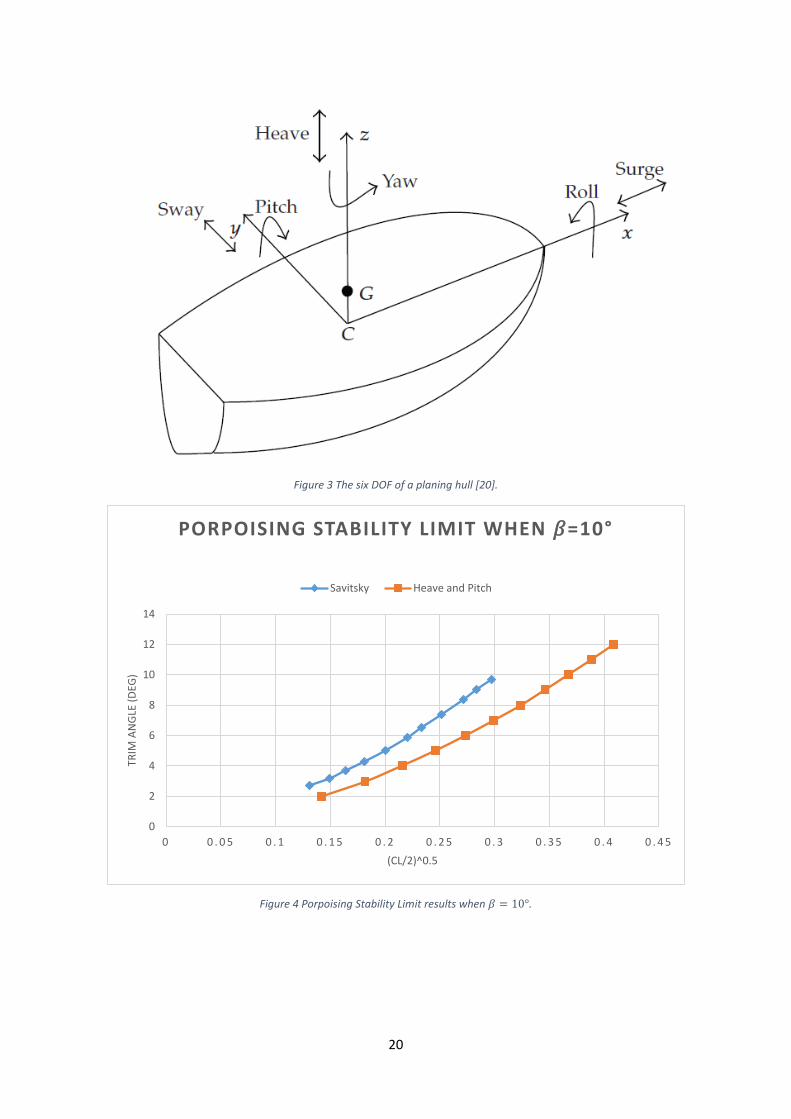
A seaplane advancing at a steady forward speed with a train of regular sea waves will move in all six degrees of freedom (DOF). This means that the plane’s motion is considered to have three translational components (surge, sway and heave) and three rotational components (roll, pitch and yaw). Figure 5 shows the six DOF system of a seaplane [20]. Eventually, in order to analytically predict the performance of a seaplane, six non-linear equations of motion must be set up and solved simultaneously. However, for a seaplane with lateral symmetry, the six equations are reduced to two sets of equations, connecting respectively, the surge, pitch and heave, and the roll, sway and yaw. In addition, as the seaplane is considered a slender body, the hydrodynamic forces associated with the translational forward motion are much smaller than the forces associated with the other motions. Not only that, but also the porpoising stability limit is studied from the equations of heave and pitch only. Consequently, the motion of seaplanes can be described by two coupled equations of heave and pitch [21].
A heaving and pitching motions of a seaplane can be seen as a two degree of freedom spring-mass system. According to Ogilvie [22], a seaplane, if given heave or pitch displacements from stationary, will rapidly oscillate several times before it comes to rest. As a result, assuming

8
that the motion is linear and harmonic, the heave and pitch equations of seaplane motion can be presented as follows:
(𝑚𝑚 + 𝐴𝐴33)ƞ̈3 + 𝐴𝐴35ƞ̈5 + 𝐵𝐵33ƞ̇3 + 𝐵𝐵35ƞ̇5 + 𝐶𝐶33ƞ3 + 𝐶𝐶35ƞ5 = 𝐹𝐹3𝑒𝑒𝑖𝑖𝑖𝑖𝑖𝑖 (1)
𝐴𝐴53ƞ̈3 + (𝐴𝐴55 + 𝐼𝐼55)ƞ̈5 + 𝐵𝐵53ƞ̇3 + 𝐵𝐵55ƞ̇5 + 𝐶𝐶53ƞ3 + 𝐶𝐶55ƞ5 = 𝐹𝐹5𝑒𝑒𝑖𝑖𝑖𝑖𝑖𝑖 (2)
Where:
𝐴𝐴𝑗𝑗𝑘𝑘 is the added-mass coefficient in the 𝑗𝑗𝑖𝑖ℎ direction due to 𝑘𝑘𝑖𝑖ℎ motion.
𝐵𝐵𝑗𝑗𝑘𝑘 is the damping coefficient in the 𝑗𝑗𝑖𝑖ℎ direction due to 𝑘𝑘𝑖𝑖ℎ motion.
𝐶𝐶𝑗𝑗𝑘𝑘 is the hydrostatic restoring force coefficient in the 𝑗𝑗𝑖𝑖ℎ direction due to 𝑘𝑘𝑖𝑖ℎ motion.
𝐹𝐹𝑗𝑗 are the complex amplitudes of the exciting forces and moments in the 𝑗𝑗𝑖𝑖ℎ direction.
𝐹𝐹𝑗𝑗𝑒𝑒𝑖𝑖𝑖𝑖𝑖𝑖 are forces and moments given by the real part of the solution.
The determination of the coefficients and exciting forces and moments is a major problem in the analytical motion prediction. According to Brown (1971) [23], the problem can be simplified by dividing the seaplane into transverse segments and then applying a strip theory to calculate the coefficients. The added mass and damping coefficients are calculated using two-dimensional hydrodynamic theory from references [21-28].
The general solution for each of the two equations of heave and pitch has two components. The homogeneous solution and the particular integral. The homogeneous solution is obtained when the system is considered under no external excitation forces or moments. On the other hand, the particular integral is obtained when the external excitation forces and moments are considered.
First of all, the homogeneous solution of the heave and pitch equations of seaplane motion can be obtained by eliminating the right hand side of equations (1) and (2) as follows:
(𝑚𝑚 + 𝐴𝐴33)ƞ̈3 + 𝐴𝐴35ƞ̈5 + 𝐵𝐵33ƞ̇3 + 𝐵𝐵35ƞ̇5 + 𝐶𝐶33ƞ3 + 𝐶𝐶35ƞ5 = 0 (3)
𝐴𝐴53ƞ̈3 + (𝐴𝐴55 + 𝐼𝐼55)ƞ̈5 + 𝐵𝐵53ƞ̇3 + 𝐵𝐵55ƞ̇5 + 𝐶𝐶53ƞ3 + 𝐶𝐶55ƞ5 = 0 (4)
If a steady-state solution is assumed, then the heave and pitch can have the following forms:
ƞ3 = 𝑍𝑍0𝑒𝑒𝜆𝜆𝑖𝑖 (5)
ƞ5 = 𝜃𝜃0𝑒𝑒𝜆𝜆𝑖𝑖 (6)
If equations (5) and (6) and substituted in equations (3) and (4), the following equations will be obtained:
(𝑚𝑚 + 𝐴𝐴33)𝜆𝜆2𝑍𝑍0 + 𝐴𝐴35𝜃𝜃0𝜆𝜆2 + 𝐵𝐵33𝜆𝜆 𝑍𝑍0 + 𝐵𝐵35𝜆𝜆 𝜃𝜃0 + 𝐶𝐶33𝑍𝑍0 + 𝐶𝐶35𝜃𝜃0 = 0 (7)
𝐴𝐴53𝜆𝜆2𝑍𝑍0 + (𝐴𝐴55 + 𝐼𝐼55)𝜆𝜆2𝜃𝜃0 + 𝐵𝐵53𝜆𝜆 𝑍𝑍0 + 𝐵𝐵55𝜆𝜆 𝜃𝜃0 + 𝐶𝐶53𝑍𝑍0 + 𝐶𝐶55𝜃𝜃0 = 0 (8)

9
In the form of a matrix, the two equations can be expressed as follows:
�(𝑚𝑚 + 𝐴𝐴33)𝜆𝜆2 + 𝐵𝐵33𝜆𝜆 + 𝐶𝐶33 𝐴𝐴35𝜆𝜆2 + 𝐵𝐵35𝜆𝜆 + 𝐶𝐶35
𝐴𝐴53𝜆𝜆2 + 𝐵𝐵53𝜆𝜆 + 𝐶𝐶53 (𝐴𝐴55 + 𝐼𝐼55)𝜆𝜆2 + 𝐵𝐵55𝜆𝜆 + 𝐶𝐶55� �𝑍𝑍0𝜃𝜃0
� = �00� (9)
For non-trivial solutions of 𝑍𝑍0 and 𝜃𝜃0, the determinant of equation (9) is set to be zero. The characteristic equation can then be written in the following form:
𝑎𝑎𝜆𝜆4 + 𝑏𝑏𝜆𝜆3 + 𝑐𝑐𝜆𝜆2 + 𝑑𝑑 𝜆𝜆 + 𝑒𝑒 = 0 (10)
Where:
𝑎𝑎 = [(𝑚𝑚 + 𝐴𝐴33)(𝐴𝐴55 + 𝐼𝐼55) − 𝐴𝐴35𝐴𝐴53] (11)
𝑏𝑏 = [(𝑚𝑚 + 𝐴𝐴33)𝐵𝐵55 + 𝐵𝐵33(𝐴𝐴55 + 𝐼𝐼55) − 𝐴𝐴35𝐵𝐵53 − 𝐵𝐵35𝐴𝐴53] (12)
𝑐𝑐 = [(𝑚𝑚 + 𝐴𝐴33)𝐶𝐶55 + 𝐵𝐵33𝐵𝐵55 + 𝐶𝐶33(𝐴𝐴55 + 𝐼𝐼55) − 𝐴𝐴35𝐶𝐶53 − 𝐵𝐵35𝐵𝐵53 − 𝐶𝐶35𝐴𝐴53] (13)
𝑑𝑑 = [𝐵𝐵33𝐶𝐶55 + 𝐶𝐶33𝐵𝐵55 − 𝐵𝐵35𝐶𝐶53 − 𝐶𝐶35𝐵𝐵53] (14)
𝑒𝑒 = [𝐶𝐶33𝐶𝐶55 − 𝐶𝐶35𝐶𝐶53] (15)
Equation (10) is the fourth order characteristic equation of the system. This equation is solved to obtain four roots. The characteristics of motion of the seaplane will depend on the nature of the roots of this equation. In order to solve equation (10), a visual basic program has been created to solve the equations of the coefficients of added mass (𝐴𝐴𝑗𝑗𝑘𝑘), damping (𝐵𝐵𝑗𝑗𝑘𝑘) and restoring forces (𝐶𝐶𝑗𝑗𝑘𝑘). The program code is illustrated in appendix A. The solution obtained consists of two real roots and two complex conjugate roots. As a result, the homogeneous solutions obtained for the two equations are as follows:
ƞ3h = 𝑍𝑍01𝑒𝑒−7.35𝑖𝑖 + 𝑍𝑍02𝑒𝑒−9.4𝑖𝑖 + 𝑒𝑒3.8𝑖𝑖(𝑍𝑍03𝑒𝑒𝑖𝑖1.836𝑖𝑖 + 𝑍𝑍04𝑒𝑒−𝑖𝑖1.836𝑖𝑖) (16)
ƞ5h = 𝜃𝜃01𝑒𝑒−7.35𝑖𝑖 + 𝜃𝜃02𝑒𝑒−9.4𝑖𝑖 + 𝑒𝑒3.8𝑖𝑖(𝜃𝜃03𝑒𝑒𝑖𝑖1.836𝑖𝑖 + 𝜃𝜃04𝑒𝑒−𝑖𝑖1.836𝑖𝑖) (17)
In addition to that, the particular integrals of the two equations have the following form:
ƞ3p = 𝑃𝑃1 cos(𝜔𝜔𝜔𝜔) + 𝑃𝑃2 sin(𝜔𝜔𝜔𝜔) (18)
ƞ5p = 𝑃𝑃3 cos(𝜔𝜔𝜔𝜔) + 𝑃𝑃4 sin(𝜔𝜔𝜔𝜔) (19)
Then, the solution of the two equations of heave and pitch can be obtained by adding the homogeneous solution and the particular integral together as follows:
�ƞ3ƞ5� = �
ƞ3hƞ5h� + �𝑃𝑃1𝑃𝑃3
� cos(𝜔𝜔𝜔𝜔) + �𝑃𝑃2𝑃𝑃4� sin(𝜔𝜔𝜔𝜔) (20)
In the case where the external waves are assumed to have the same frequency as one of the components of the homogeneous solution, say 𝜔𝜔 = 𝜔𝜔1 = 1.836, then the general solution reads as:
10
�ƞ3ƞ5� = �
ƞ3hƞ5h� + �𝑃𝑃1𝑃𝑃3
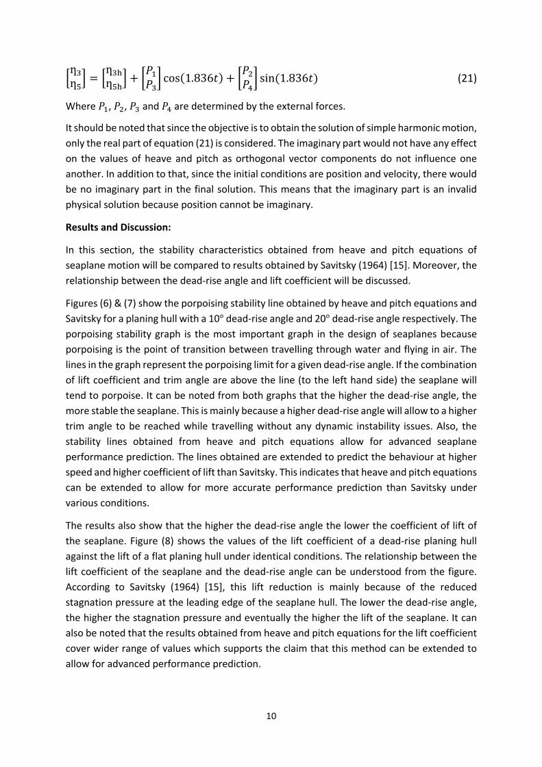
� cos(1.836𝜔𝜔) + �𝑃𝑃2𝑃𝑃4� sin(1.836𝜔𝜔) (21)
Where 𝑃𝑃1, 𝑃𝑃2, 𝑃𝑃3 and 𝑃𝑃4 are determined by the external forces.
It should be noted that since the objective is to obtain the solution of simple harmonic motion, only the real part of equation (21) is considered. The imaginary part would not have any effect on the values of heave and pitch as orthogonal vector components do not influence one another. In addition to that, since the initial conditions are position and velocity, there would be no imaginary part in the final solution. This means that the imaginary part is an invalid physical solution because position cannot be imaginary.
Results and Discussion:
In this section, the stability characteristics obtained from heave and pitch equations of seaplane motion will be compared to results obtained by Savitsky (1964) [15]. Moreover, the relationship between the dead-rise angle and lift coefficient will be discussed.
Figures (6) & (7) show the porpoising stability line obtained by heave and pitch equations and Savitsky for a planing hull with a 10° dead-rise angle and 20° dead-rise angle respectively. The porpoising stability graph is the most important graph in the design of seaplanes because porpoising is the point of transition between travelling through water and flying in air. The lines in the graph represent the porpoising limit for a given dead-rise angle. If the combination of lift coefficient and trim angle are above the line (to the left hand side) the seaplane will tend to porpoise. It can be noted from both graphs that the higher the dead-rise angle, the more stable the seaplane. This is mainly because a higher dead-rise angle will allow to a higher trim angle to be reached while travelling without any dynamic instability issues. Also, the stability lines obtained from heave and pitch equations allow for advanced seaplane performance prediction. The lines obtained are extended to predict the behaviour at higher speed and higher coefficient of lift than Savitsky. This indicates that heave and pitch equations can be extended to allow for more accurate performance prediction than Savitsky under various conditions.
The results also show that the higher the dead-rise angle the lower the coefficient of lift of the seaplane. Figure (8) shows the values of the lift coefficient of a dead-rise planing hull against the lift of a flat planing hull under identical conditions. The relationship between the lift coefficient of the seaplane and the dead-rise angle can be understood from the figure. According to Savitsky (1964) [15], this lift reduction is mainly because of the reduced stagnation pressure at the leading edge of the seaplane hull. The lower the dead-rise angle, the higher the stagnation pressure and eventually the higher the lift of the seaplane. It can also be noted that the results obtained from heave and pitch equations for the lift coefficient cover wider range of values which supports the claim that this method can be extended to allow for advanced performance prediction.

11
Conclusion:
In conclusion, this paper has discussed the analytical methods used for seaplanes performance prediction and defined the weaknesses in each method. Also, the motion characteristics of seaplane have been studied and the operating ranges specified.
The paper has highlighted most of the conventional analytical methods used for planing hulls performance prediction. It has been argued that the methods lack the ability to predict the stability limits of planing hulls which is a very important issue especially in the design stage. Also, the methods are only valid under certain geometry and conditions. Moreover, all of the methods are used to study the behaviour of planing hulls under steady state conditions only. No method takes the aerodynamic forces into consideration.
On the other hand, heave and pitch equations of seaplane motion have the ability to predict the stability limits of seaplanes and more importantly, this method can predict the performance for higher-speed regime than any of the other methods. It has also been shown that this approach can be expanded to allow for more advanced performance prediction and include non-linear effects.
12
References:
[1] Rozhdestvensky, K. (2006). Wing-in-ground effect vehicles. Progress in Aerospace Sciences, 42(3), pp.211-283.
[2] Baird, N. (1998). The World Fast Ferry Market. Melbourne Australia. Baird Publications.
[3] Faltinsen, O. (2010). Hydrodynamics of High-Speed Marine Vehicles. Leiden: Cambridge University Press, p.344.
[4] Dala, L. (2015). Dynamic Stability of a Seaplane in Takeoff. Journal of Aircraft, 52(3), pp.964-971.
[5] Yun, L., Bliault, A. and Doo, J. (2010). WIG craft and ekranoplan. New York: Springer.
[6] Priyanto, A., Maimun, A., Noverdo, S., Saeed, J., Faizal, A. and Waqiyuddin, M. (2012). A Study on Estimation of Propulsive Power for Wing in Ground Effect (WIG) Craft to Take-off. Jurnal Teknologi, 59(1).
[7] Baker, G. (1912). Some Experiments in Connection with the Design of Floats for Hydro-Aeroplanes. ARC R&M.
[8] Sottorf, W. (1932). Experiments with Planing Surfaces. NACA TM 661 and NACA TM 739.
[9] Shoemaker, J. (1934). Tanks Tests of Flat and Vee-Bottom Planing Surfaces. NACA TM 848.
[10] Sambraus, A. (1938). Planing Surfaces Tests at Large Froude Numbers - Airfoil Comparison. NACA TM 509.
[11] Sedov, L. (1947). Scale Effect and Optimum Relation for Sea Surface Planing. NACA TM 1097.
[12] Locke, F. (1948). Tests of a Flat Bottom Planing Surface to Determine the Inception of Planing. US Navy Department, BUAER, Research Division Report No.1096.
[13] Korvin-Kroukovsky, B., Savitsky, D. and Lehman, W. (1949). Wetted Area and Center of pressure of Planing Surfaces. Stevens Institute of Technology, Davidson Laboratory Report No. 360.
[14] Murray, A.B. (1950). The hydrodynamic of Planing Hulls. New England SNAME Meeting 1950. Jersey City (USA): SNAME.
[15] Savitsky, D. (1964). Hydrodynamic Design of Planing Hulls. Marine Technology, 1(1), pp.71-95.
[16] Almeter, J. (1993). Resistance Prediction of Planing Hulls: State of the Art. Marine Technology, 30(4), pp.297-307.

13
[17] Iacono, M. (2015). Hydrodynamics of Planing Hulls by CFD. M.Sc. University of Naples, Italy.
[18] Payne, P. (1995). Contributions to planing theory. Ocean Engineering, 22(7), pp.699-729.
[19] Shuford, C. (1958). A Theoretical and Experimental Study of Planing Surfaces Including effects of Cross section and Plan Form. National Advisory Committee for Aeronautics Report 1355.
[20] Ibrahim, R. and Grace, I. (2010). Modeling of Ship Roll Dynamics and Its Coupling with Heave and Pitch. Mathematical Problems in Engineering, 2010, pp.1-32.
[21] Salvesen, N., Tuck, E. and Faltinsen, O. (1970). Ship Motions and Sea Loads. The Society of Naval Architects and Marine Engineers.
[22] Ogilvie, T. (1969). The Development of Ship-Motion theory. Ann Arbor, Michigan, USA: Department of naval Architecture and Marine engineering, College of Engineering, The University of Michigan.
[23] Brown, P. (1971). An Experimental and Theoretical Study of Planing Surfaces with trim Flaps. Hoboken, N.J: Stevens Institute of Technology, Report SIT-DL-71-1462.
[24] Fossen, T. (2011). Handbook of marine craft hydrodynamics and motion control. 1st ed. Chichester, West Sussex: John Wiley & Sons.
[25] Lewis, E. (1989). Principles of naval architecture. Jersey City, NJ, USA: Society of Naval Architects and Marine Engineers.
[26] Korvin-Kroukovsky, B. (1955). Investigation of ship motions in regular waves. The Society of Naval Architects and Marine Engineers.
[27] Fossen, T. (1994). Guidance and control of ocean vehicles. West Sussex, England: John Wiley & Sons.
[28] Ito, K., Dhaene, T., Hirakawa, Y., Hirayama, T. and Sakurai, T. (2016). Longitudinal Stability Augmentation of Seaplanes in Planing. Journal of Aircraft, 53(5), pp.1332-1342.

14
Appendix A:
The solution of the heave and pitch equations was obtained by using Visual Basic. The equations used for the added mass, damping and restoring forces and moments coefficients were obtained from reference [28]. The VB code developed is as follows:
Option Explicit On Public Class Form1 Private Sub solve_Click(sender As Object, e As EventArgs) Handles solve.Click Dim W, rhu, U, B, beta As Double Dim CLo As Double Dim d As Double Dim lambdaw As Double Dim tau As Double Dim FnB As Double Dim Lk As Double Dim Lc As Double Dim Vcg As Double Dim Lcg As Double Lcg = Val(Lcgtxt.Text) W = Val(weighttxt.Text) rhu = Val(densitytxt.Text) U = Val(speedtxt.Text) B = Val(beamtxt.Text) beta = Val(deadrisetxt.Text) tau = Val(tautxt.Text) FnB = U / ((9.8 * B) ^ 0.5) froudetxt.Text = FnB Lk = (B * Math.Tan(beta * Math.PI / 180)) / (2 * Math.Tan(tau * Math.PI / 180)) Lktxt.Text = Lk d = Lk * Math.Sin(tau * Math.PI / 180) drafttxt.Text = d Lc = Lk - ((B * Math.Tan(beta * Math.PI / 180)) / (Math.PI * Math.Tan(tau * Math.PI / 180))) Lctxt.Text = Lc lambdaw = (Lk + Lc) / (2 * B) Dim CLbeta As Double CLbeta = (W / (0.5 * rhu * U * U * B * B)) CLbetatxt.Text = CLbeta CLo = (tau ^ 1.1) * ((0.012 * (lambdaw ^ 0.5)) + (0.0055 * (lambdaw ^ 2.5) / (FnB * FnB))) CLotxt.Text = CLo

15
lambdawtxt.Text = lambdaw Dim Lp As Double Lp = Lcg Lptxt.Text = Lp Dim x1 As Double x1 = (-1 / ((Math.Sin(tau * Math.PI / 180)) * B)) Dim x2 As Double x2 = (tau ^ 1.1) * ((0.006 * (lambdaw ^ -0.5)) + (0.01375 * (lambdaw ^ 1.5) / FnB * FnB)) * x1 Dim C33 As Double C33 = (0.5 * rhu * U * U * B) * (-B) * x2 * (1 - (0.0039 * beta * (CLo ^ -0.4))) C33txt.Text = C33 Dim x3 As Double Dim Zwl As Double Zwl = (Vcg * Math.Cos(tau * Math.PI / 180)) - ((Lk - Lcg) * Math.Sin(tau * Math.PI / 180)) x3 = (-Vcg / (B * (Math.Sin(tau * Math.PI / 180)) ^ 2)) + ((Zwl / (B * (Math.Sin(tau * Math.PI / 180)) ^ 2)) * (Math.Cos(tau * Math.PI / 180))) + ((0.25 * Math.Tan(beta * Math.PI / 180)) / (1.57 * (tau) ^ 2)) Dim x4 As Double x4 = (1.1 * (180 / Math.PI) ^ 1.1) * ((tau * Math.PI / 180) ^ 0.1) * ((0.012 * (lambdaw ^ 0.5)) + (0.0055 * (lambdaw ^ 2.5) / FnB * FnB)) + ((tau ^ 1.1) * ((0.006 * (lambdaw ^ -0.5)) + (0.01375 * (lambdaw ^ 1.5) / FnB * FnB))) * x3 Dim C35 As Double C35 = (0.5 * rhu * U * U * B * B) * (-B) * x4 * (1 - (0.0039 * beta * (CLo ^ -0.4))) C35txt.Text = C35 Dim x5 As Double x5 = (0.75 - (((15.63 * FnB * FnB / lambdaw * lambdaw) + 2.39) / ((5.21 * FnB * FnB / lambdaw * lambdaw) + 2.39) ^ 2)) Dim x6 As Double x6 = (-C33 / (0.5 * rhu * U * U * B)) Dim C53 As Double C53 = -(x5 * B * x1 * CLbeta) * (0.5 * rhu * U * U * B * B) C53txt.Text = C53 Dim C55 As Double C55 = -(x5 * x3 * CLbeta * (0.5 * rhu * U * U * B * B * B)) C55txt.Text = C55 Dim k As Double k = (0.125 * 3.14 * B * B * (1 - (beta * 4.56 * (10 ^ -3)))) / (d * d) Dim A33a As Double A33a = (rhu * B * B * B * k * (Math.Tan(beta * Math.PI / 180)) ^ 3) / (37.68 * (tau * Math.PI / 180)) Dim c1 As Double c1 = (0.6369 * (Math.Tan(beta * Math.PI / 180)) ^ 2) * k Dim A33b As Double A33b = (rhu * B * B * c1 * Lc * 0.3925) Dim A33 As Double A33 = A33a + A33b A33txt.Text = A33

16
Dim XG As Double XG = Lk - Lcg Dim A35a As Double A35a = (A33a * XG) - ((k * rhu * B * B * B * B / 64) * ((Math.Tan(beta * Math.PI / 180)) ^ 4) / (2.4649 * (tau * Math.PI / 180) ^ 2)) Dim A35b As Double Dim Xs As Double Xs = (B * Math.Tan(beta * Math.PI / 180)) / (3.14 * (tau * Math.PI / 180)) A35b = (A33b * XG) - (rhu * B * B * B * B * c1 * 0.19625 * (((Lk / B) ^ 2) - ((Xs / B) ^ 2))) Dim A35 As Double A35 = A35a + A35b Dim A53 As Double A53 = A35 A35txt.Text = A35 A53txt.Text = A53 Dim A55a As Double Dim A55b As Double Dim A55 As Double A55a = ((k * rhu * (B ^ 5) * ((Math.Tan(beta * Math.PI / 180)) ^ 5)) / (619.18288 * ((tau * Math.PI / 180) ^ 3))) - (k * XG * rhu * B * B * B * B * B * ((Math.Tan(beta * Math.PI / 180)) ^ 4) / (50.24 * B * ((tau * Math.PI / 180) ^ 2))) + ((((XG / B) ^ 2) * rhu * B * B * B * B * B * A33a) / (rhu * B * B * B)) A55b = (rhu * B * B * B * B * B * c1 * 0.13083 * (((Lk / B) ^ 3) - ((Xs / B) ^ 3))) - (c1 * 0.3925 * rhu * B * B * B * B * B * (XG / B) * (((Lk / B) ^ 2) - ((Xs / B) ^ 2))) + (((XG / B) ^ 2) * (A33b * B * B)) A55 = A55a + A55b A55txt.Text = A55 Dim x7 As Double x7 = (0.0132 * ((57.324) ^ 1.1) * ((tau * Math.PI / 180) ^ 0.1) * (lambdaw ^ 0.5)) Dim x8 As Double x8 = (x7) * (1 - (0.0039 * beta * ((CLo ^ -0.4)))) Dim B33 As Double B33 = (rhu * B * B * B * ((9.8 / B) ^ 0.5) * 0.5 * FnB * x8) B33txt.Text = B33 Dim B35 As Double Dim a33xt As Double a33xt = k * rhu * (((B * Math.Tan(beta * Math.PI / 180)) / 2) ^ 2) B35 = (U * A33) - (U * Lcg * a33xt) B35txt.Text = B35 Dim B53 As Double B53 = (B33 * B * 0.75 * lambdaw) - (B33 * Lcg) B53txt.Text = B53 Dim B55 As Double B55 = U * Lcg * Lcg * a33xt B55txt.Text = B55 Dim I55 As Double I55 = (W / 49) * ((Lcg ^ 2) + (Vcg ^ 2)) Dim aa, bb, cc, dd, ee As Double aa = (((W / 9.8) + A33) * (A55 + I55)) - (A35 * A53) bb = ((W / 9.8 + A33) * (B55)) + ((B33) * (A55 + I55)) - (A35 * B53) - (B35 * A53) atxt.Text = aa
17
btxt.Text = bb cc = (((W / 9.8) + A33) * (C55)) + (B33 * B55) + ((C33) * (A55 + I55)) - (A35 * C53) - (B35 * B53) - (C35 * A53) ctxt.Text = cc dd = ((B33 * C55) + (C33 * B55) - (B35 * C53) - (C35 * B53)) dtxt.Text = dd ee = (C33 * C55) - (C35 * C53) etxt.Text = ee End Sub Private Sub Button1_Click(sender As Object, e As EventArgs) Handles Button1.Click weighttxt.Text = 264600 densitytxt.Text = 1026 speedtxt.Text = 20.5 beamtxt.Text = 4.27 deadrisetxt.Text = 10 tautxt.Text = 4 Vcgtxt.Text = 0.607 Lcgtxt.Text = 8.84 End Sub End Class

18
Figures:
Figure 1 Seaplane operating phases.
Figure 2 The three operating ranges of seaplanes [5].
19
Figure 3 Seaplane hull in displacement and planing modes [6].
Figure 2 Planing hull characteristics [15].
20
Figure 3 The six DOF of a planing hull [20].
Figure 4 Porpoising Stability Limit results when 𝛽𝛽 = 10°.
0
2
4
6
8
10
12
14
0 0 . 0 5 0 . 1 0 . 1 5 0 . 2 0 . 2 5 0 . 3 0 . 3 5 0 . 4 0 . 4 5
TRIM
AN
GLE
(DEG
)
(CL/2)^0.5
PORPOISING STABILITY LIMIT WHEN 𝛽𝛽=10°
Savitsky Heave and Pitch

21
Figure 7 Porpoising Stability Limit results when 𝛽𝛽 = 20°.
Figure 8 Lift coefficients of a dead-rise planing hull.
0
2
4
6
8
10
12
14
0 0 . 0 5 0 . 1 0 . 1 5 0 . 2 0 . 2 5 0 . 3 0 . 3 5
TRIM
AN
GLE
(DEG
)
(CL/2)^0.5
PORPOISING STABILIY LIMIT WHEN 𝛽𝛽=20°
Savitsky Heave and Pitch
0
0.02
0.04
0.06
0.08
0.1
0.12
0.14
0.16
0.18
0 0 . 0 2 0 . 0 4 0 . 0 6 0 . 0 8 0 . 1 0 . 1 2 0 . 1 4 0 . 1 6 0 . 1 8 0 . 2
CL𝛽𝛽
CLO
CL𝛽𝛽 VS CLO
Heave and Pitch at β =10° Heave and Pitch at β =20°
Savitsky at β =10° Savitsky at β =20°