Embed Size (px)
Citation preview

i
COURSE OBJECTIVES CHAPTER 2
2. HULL FORM AND GEOMETRY 1. Be familiar with ship classifications 2. Explain the difference between aerostatic, hydrostatic, and hydrodynamic support 3. Be familiar with the following types of marine vehicles: displacement ships,
catamarans, planing vessels, hydrofoil, hovercraft, SWATH, and submarines 4. Learn Archimedes Principle in word and mathematical form 5. Calculate problems using Archimedes Principle 6. Read, interpret, and relate the body plan, half-breadth plan, and sheer plan
including naming the lines found in each plan 7. Relate the information in a ship's lines plan to a Table of Offsets 8. Be familiar with the following hull form terminology: a. After Perpendicular (AP), Forward Perpendiculars (FP) and midships b. Length Between Perpendiculars (Lpp ) and Length Overall (LOA) c. Keel (K), Depth (D), Draft (T), Mean Draft (Tm), Freeboard and Beam (B) d. Flare, Tumble home and Camber e. Centerline, Baseline and Offset 9. Define, compare, and contrast “centroid” and “center of mass” 10. State the physical significance and location of the center of buoyancy (B) and
center of flotation (F); locate these points using LCB, VCB, TCB, TCF, and LCF 11. Use Simpson’s 1st Rule to calculate the following given a Table of Offsets: a. Waterplane Area (Awp) or (WPA) b. Sectional Area (Asect) c. Submerged Volume (∇) d. Longitudinal Center of Flotation (LCF) 12. Read and use a ship's Curves of Form to find hydrostatic properties and be
knowledgeable about each of the properties on the Curves of Form 13. Calculate trim given Taft and Tfwd and understand its physical meaning

2-1
2.1 Introduction to Ships and Naval Engineering Ships are the single most expensive product a nation produces for defense, commerce, research, or nearly any other function. If we are to use such expensive instruments wisely, we must understand how and why they operate the way they do. Ships employ almost every type of engineering system imaginable. Structural networks hold the ship together and protect its contents and crew. Machinery propels the ship and provides for all of the needs of the ship's inhabitants. Every need of every member of the crew must be provided for: cooking, eating, trash disposal, sleeping, and bathing. The study of ships is a study of systems engineering. There are many types of ships from which to choose, and each type has advantages and disadvantages. Factors which may influence the ship designer's decisions or the customer's choices include: cost, size, speed, seakeeping, radar signature, draft, maneuverability, stability, and any number of special capabilities. The designer must weigh all of these factors, and others, when trying to meet the customer's specifications. Most ships sacrifice some characteristics, like low cost, for other factors, like speed. The study of naval engineering is the merging of the art and craft of ship building with the principles of physics and engineering sciences to meet the requirements of a naval vessel. It encompasses research, development, design, construction, operation, maintenance, and logistical support of naval vessels. This introductory course in naval engineering is meant to give each student an appreciation in each of the more common areas of study. It is meant as a survey course that will give some good practical knowledge to every officer assigned to naval service on land, sea or in the air. Shipbuilding and design is a practice that dates back to the first caveman who dug a hole
in a log to make a canoe. The birth of “modern” shipbuilding, that is the merging of art and science, is attributed to Sir Anthony Deane, a shipwright who penned his treatise, Doctrine of Naval Architecture in 1670.
!

2-2
2.2 Categorizing Ships The term “ship” can be used to represent a wide range of vessels operating on, above or below the surface of the water. To help organize this study, ships are often categorized into groups based on either usage, means of support while in operation, or both. A list of classification by usage might include the following.
• Merchant Ships: These ships are intended to earn a profit in the distribution of goods. A cash flow analysis is done of income versus costs in the calculation of a rate of return on the investment. Engineering economy studies must include receipts earned, acquisition costs, operating and maintenance costs, and any salvage value remaining when the ship is sold in a time value of money study.
• Naval and Coast Guard Vessels: Classified as combatants or auxiliaries. These ships
tend to be extremely expensive because their missions require many performance capabilities such as speed, endurance, weapons payload, ability to operate and survive in hostile environments and reliability under combat conditions.
• Recreational and Pleasure Ships: Personal pleasure craft and cruise liners are a
specialized class of ships that are run to earn a profit by providing recreation services to the general public. Comfort and safety are of utmost importance.
• Utility Tugs: Designed for long operation and easy maintenance with a no frills
approach.
• Research and Environmental Ships: Highly specialized equipment must be kept and often deployed into and out of the water.
• Ferries: People and vehicles must load and unload with efficiency and safety in
accordance with a strict time schedule in all weather conditions. Ships can also be classified by the means of physical support while in operation. Three broad classifications that are frequently used by naval architects are shown in Figure 2.1, reproduced from “Introduction to Naval Architecture” by Gillmer and Johnson.
• Aerostatic Support
• Hydrodynamic Support
• Hydrostatic Support

2-3
Seagoing Vessels (Surface, Surface Effect, Sub-surface)
Figure 2.1 Categories of Seagoing Vessels According to Mode of Support

2-4
2.2.1 Aerostatic Support Aerostatic support is achieved when the vessel rides on a cushion of air generated by lift fans. These vessels tend to be lighter weight and higher speed vessels. The two basic types of vessels supported aerostatically are air cushion vehicle (ACV) and surface effect ships (SES). 2.2.1.1 Air Cushion Vehicles (ACVs) Air Cushion Vehicles (ACVs) or hovercraft continuously force air under the vessel allowing some of the air to escape around the perimeter as new air is forced downwards. They are usually propelled forward by airplane propeller type devices above the surface of the water with rudders behind the air flow to control the vessel. The Navy utilizes some hovercraft as LCACs (Landing Craft Air Cushion vehicles) because of this ability. Their use has opened over 75% of the world's coastline to amphibious assault compared with 5% with conventional landing craft. Pro: Amphibious operations; fast Con: Very expensive for their payload capacity; low directional stability with air rudders 2.2.1.2 Surface Effect Ship (SES) The Surface Effect Ship (SES) or Captured Air Bubble (CAB) craft, is similar to the ACV due to its use of a cushion of air to lift the vessel. However, the SES has rigid side walls that extend into the water, providing directional stability and hydrostatic or hydrodynamic lift. They are usually propelled by water jets or super-cavitating propellers. There were two SESs operated by the USN from about 1972-1975. They were the SES-100 A and B models (displacement 100 LT) capable of traveling at speeds of over 80 knots. The SES-100 was meant as an experimental platform carrying only 6 to 7 people. More recently, SES-200 (displacement 200 LT) was retired from the Naval Air Station at Patuxent River. Several European Navies operate SESs as fast patrol boats, designed to operate in coastal waters. Pro: Less air lift requirement, more directionally stable, and more payload (compared to ACV) Con: Not amphibious; expensive for their payload capacity 2.2.2 Hydrodynamic Support Hydro is the prefix for water and dynamic indicates movement. The two basic types of vessels supported hydrodynamically are planing vessels and hydrofoils. 2.2.2.1 Planing Vessels Planing vessels use the hydrodynamic pressures developed on the hull at high speeds to support the ship. They ride comfortably in smooth water, but when moving through waves, planing vessels ride very roughly, heavily stressing both the vessel structure and passengers. This was particularly true of older types which used relatively flat bottom hulls. Modifications to the basic hull form, such as deep V-shaped sections, have helped to alleviate this problem somewhat.

2-5
These factors above serve to limit the size of planing vessels. However, these ships are used in a variety of roles such as pleasure boats, patrol boats, missile boats, and racing boats. At slow speeds the planing craft acts like a displacement ship and is supported hydrostatically. Pro: Fast 50+ kt; comfortable ride in smooth seas Con: Large engines for size; slam into waves in moderate/high seas; limited capacity 2.2.2.2 Hydrofoils Hydrofoil craft are supported by underwater foils, not unlike the wings of an aircraft. At high speeds these underwater surfaces develop lift and raise the hull out of the water. Bernoulli’s Principle is often used to explain how a wing develops lift. Compared to planing boats, hydrofoils experience much lower vertical accelerations in moderate sea states making them more comfortable to ride. The hydrofoil can become uncomfortable or even dangerous in heavy sea states due to the foils breaking clear of the water and the hull impacting the waves. If the seaway becomes too rough the dynamic support is not used, and the ship becomes a displacement vessel. The need for the hydrofoils to produce enough upward force to lift the ship out of the water places practical constraints on the vessel's size. Therefore, the potential crew and cargo carrying capacity of these boats is limited. Hydrofoils are also very expensive for their size in comparison to conventional displacement vessels. The U.S. Navy formerly used hydrofoils as patrol craft and to carry anti-ship missiles (Pegasus Class), but does not use them anymore due to their high acquisition and maintenance costs. Pro: Fast 40-60 kt; smoother ride in moderate seas (compared to planing) Con: Expensive for their size; dangerous in heavy seas; limited capacity 2.2.3 Hydrostatic Support Hydrostatically supported vessels are by far the most common type of waterborne craft. They describe any vessel that is supported by “Archimedes Principle.” Word definition of Archimedes Principle
“An object partially or fully submerged in a fluid will experience a resultant vertical force equal in magnitude to the weight of the volume of fluid displaced by the object.”
This force is often referred to as the “buoyant force” or the “force of buoyancy.” Archimedes Principle can be written in mathematical format as follows.
∇= gFB ρ

2-6
Where: FB is the magnitude of the resultant buoyant force (lb) ρ is the density of the fluid (lb-s2/ft4)
g is the acceleration due to gravity (32.17 ft/s2) ∇ is the volume of fluid displaced by the object in (ft3)
If you do not understand the units of density (lb-s2/ft4) ask your instructor to explain
them. Example 2.1 Calculate the buoyant force being experienced by a small boat with a submerged
volume of 20 ft3 when floating in seawater. (ρsalt = 1.99 lb-s2/ft4).
lbFftftftlbgF
B
B
280,120sec17.32sec99.1 3242
=⋅⋅=∇= ρ
Example 2.2 What is the submerged volume of a ship experiencing a buoyant force of 4000 LT
floating in fresh water? (ρfresh = 1.94 lb-s2/ft4 , 1 LT = 2240 lb)
3
24
2
570,143sec17.32sec94.1
22404000
ft
ftft
lbLT
lbLT
gF
gF
B
B
=∇
⋅
⋅==∇
∇=
ρ
ρ
2.2.3.1 Displacement Ships Hydrostatically supported ships are referred to as “displacement ships”, since they float by displacing their own weight in water, according to Archimedes Principle. These are the oldest form of ships coming in all sizes and being used for such varied purposes as hauling cargo, bulk oil carrying, launching and recovering aircraft, transporting people, fishing, and war fighting. Displacement hulls have the advantage of being a very old and common type of ship. Therefore, many aspects of their performance and cost have been well studied. In comparison to other types of vessels the cost of displacement ships is fairly low with respect to the amount of payload they can carry. Pro: Vast experience in design and operation; lower cost; high payload Con: Limited speed; some difficulty seakeeping in waves (compared to SWATH) 2.2.3.2 SWATH A special displacement ship is the Small Waterplane Area Twin Hull (SWATH). Most of the underwater volume in the SWATH ship is concentrated well below the water's surface as shown in Figure 2.1. This gives them very good seakeeping characteristics. They also have a large open deck and are therefore useful in a variety of applications requiring stable platforms and a large
!

2-7
expanse of deck space. SWATH vessels are currently utilized as cruise ships, ferries, research vessels, and towed array platforms. These vessels present the designer with structural problems differing from other ships, particularly with respect to transverse bending moments. Pro: Excellent seakeeping in waves; large deck for operations Con: Deep draft; higher cost; structural loading 2.2.3.3 Submarines Submarines are hydrostatically supported, but above 3 to 5 knots depth control can be achieved hydrodynamically due to the lift created by the submarines planes and the body of the hull. Submarines have typically been used as weapons of war, but lately have also seen some non-military application. Some submarines are being designed for the purpose of viewing underwater life and reefs, for example. Unmanned submersibles have been used for scientific purposes, such as finding the Titanic, as well as a wide variety of oceanographic research. There are many differences between the engineering problems faced by the surface ship designer and those faced by the submarine designer. Many of these differences will be covered in the last chapter of this course.

2-8
2.3 The Traditional Way to Represent the Hull Form A ship's hull is a very complicated 3 dimensional shape. With few exceptions, an equation cannot be written that fully describes the shape of a ship. Therefore, engineers have placed great emphasis on the graphical description of hull forms. Until very recently, most of this work was done by hand. Today high-speed digital computers assist the engineer with the drawings, but they are not substitutes for imagination and judgment. Traditionally, the ship's hull form is represented graphically by a lines drawing. The lines drawings consist of the intersection of the hull with a series of planes. The planes are equally spaced in each of the three dimensions. Planes in one dimension will be perpendicular to planes in the other two dimensions. We say that the sets of planes are mutually perpendicular or orthogonal planes. The points of intersection of these planes with the hull results in a series of lines that are projected onto a single plane located on the front, top, or side of the ship. This results in three separate projections, or views, called the Body Plan, the Half-Breadth Plan, and the Sheer plan, respectively. Figure 2.2 displays the creation of these views. Representing a 3 dimensional shape with three orthogonal plane views is a common
practice in engineering. The engineer must be able to communicate an idea graphically so that it can be fabricated by a machinist or technician. In engineering terms, this type of mechanical drawing is referred to as an “orthographic plate” because it contains three orthogonal graphic pictures of the object. Orthographic projections are used in all engineering fields.
To visualize how a “lines drawing” works, place the ship in an imaginary rectangular box whose sides just touch the keel and sides of the ship. A viewed from the front, slice the box like a loaf of bread, and then trace each slice onto the front imaginary wall. Repeat slicing and tracing from the bottom and side, as the basis for three orthogonal projection screens. The lines to be projected result from the intersection of the hull with planes that are parallel to each of the three orthogonal planes mentioned. Refer to Figure 2.2. To measure the location of a ship’s hull, first a convenient axis and reference system must be understood. Measurements to port or starboard are measured from a centerline out to a buttock line. To measure the vertical location, distance from a baseline at the ship’s keel is determined. Each vertical spacing above this baseline is called a waterline. To measure longitudinal distance, a forward perpendicular (FP), aft perpendicular (AP), and midships are convenient reference planes. Stations or section lines are measured aft of the FP. These reference planes will be explained further and used in developing the three orthogonal lines plans
!

2-9
Figure 2.2 The Projection of Lines onto 3 Orthogonal Planes
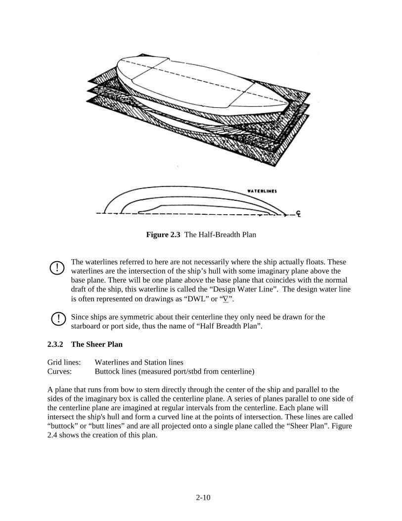
2.3.1 The Half-Breadth Plan Grid lines: Buttock lines and Station lines Curves: Waterlines (measured vertically up from baseline) The bottom of the box is a reference plane called the base plane. The base plane is usually level with the keel. A series of planes parallel and above the base plane are imagined at regular intervals, usually at every foot. Each plane will intersect the ship's hull and form a line at the points of intersection. These lines are called “waterlines” and are all projected onto a single plane called the “Half Breadth Plan.” Figure 2.3 shows the creation of this plan. Each waterline shows the true shape of the hull from the top view for some elevation above the base plane which allows this line to serve as a pattern for the construction of the ship’s framing.
2-10
Figure 2.3 The Half-Breadth Plan The waterlines referred to here are not necessarily where the ship actually floats. These
waterlines are the intersection of the ship’s hull with some imaginary plane above the base plane. There will be one plane above the base plane that coincides with the normal draft of the ship, this waterline is called the “Design Water Line”. The design water line is often represented on drawings as “DWL” or “∇”.
Since ships are symmetric about their centerline they only need be drawn for the
starboard or port side, thus the name of “Half Breadth Plan”. 2.3.2 The Sheer Plan Grid lines: Waterlines and Station lines Curves: Buttock lines (measured port/stbd from centerline) A plane that runs from bow to stern directly through the center of the ship and parallel to the sides of the imaginary box is called the centerline plane. A series of planes parallel to one side of the centerline plane are imagined at regular intervals from the centerline. Each plane will intersect the ship's hull and form a curved line at the points of intersection. These lines are called “buttock” or “butt lines” and are all projected onto a single plane called the “Sheer Plan”. Figure 2.4 shows the creation of this plan.
!
!

2-11
Each buttock line shows the true shape of the hull from the side view for some distance from the centerline of the ship. This allows them to serve as a pattern for the construction of the ship’s longitudinal framing. The centerline plane shows a special butt line called the “profile” of the ship.
Figure 2.4 The Sheer Plan The sheer plan gets its name from the idea of a sheer line on a ship. The sheer line on a
ship is the upward longitudinal curve of a ship’s deck or bulwarks. It is the sheer line of the vessel which gives it a pleasing aesthetic quality.
2.3.3 The Body Plan Grid lines: Waterlines and Buttock lines Curves: Stations or section lines (measured aft of FP) Planes parallel to the front and back of the imaginary box are called stations. A ship is typically divided into 11, 21, 31, or 41 evenly spaced stations, with larger ships having more stations. An odd number of stations results in an even number of equal blocks between the stations. The first forward station at the bow is usually labeled station number zero. This forward station is called the forward perpendicular (FP). By definition the FP is located at a longitudinal position as to intersect the stem of the ship at the DWL.
!
!
2-12
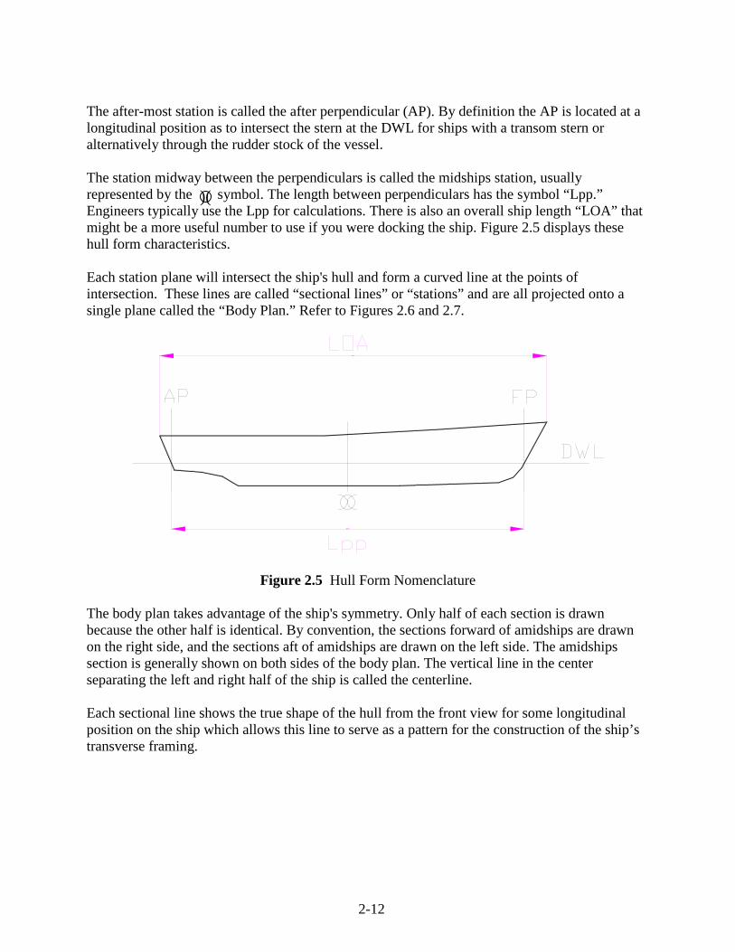
The after-most station is called the after perpendicular (AP). By definition the AP is located at a longitudinal position as to intersect the stern at the DWL for ships with a transom stern or alternatively through the rudder stock of the vessel. The station midway between the perpendiculars is called the midships station, usually represented by the symbol. The length between perpendiculars has the symbol “Lpp.” Engineers typically use the Lpp for calculations. There is also an overall ship length “LOA” that might be a more useful number to use if you were docking the ship. Figure 2.5 displays these hull form characteristics. Each station plane will intersect the ship's hull and form a curved line at the points of intersection. These lines are called “sectional lines” or “stations” and are all projected onto a single plane called the “Body Plan.” Refer to Figures 2.6 and 2.7.
Figure 2.5 Hull Form Nomenclature
The body plan takes advantage of the ship's symmetry. Only half of each section is drawn because the other half is identical. By convention, the sections forward of amidships are drawn on the right side, and the sections aft of amidships are drawn on the left side. The amidships section is generally shown on both sides of the body plan. The vertical line in the center separating the left and right half of the ship is called the centerline. Each sectional line shows the true shape of the hull from the front view for some longitudinal position on the ship which allows this line to serve as a pattern for the construction of the ship’s transverse framing.
)(

2-13
Figure 2.6 The Body Plan
Figure 2.7a Modified USNA Yard Patrol Craft Body Plan

2-14
Figure 2.7b Modified Lines Plan of the USNA Yard Patrol Craft

2-15
2.4 Table of Offsets To calculate geometric characteristics of the hull using numerical techniques, the information on the lines drawing is converted to a numerical representation in a table called the table of offsets. The table of offsets lists the distance in the y-direction from the center plane to the outline of the hull at each station and waterline. This distance is called the “offset” or “half-breadth distance.” Figure 2.8 indicates the measurement in each row and column of a table of offsets. There is enough information in the table of offsets to produce all three plans of the lines plan. Additionally, a table of offsets may be used to calculate geometric properties of the hull, such as sectional area, waterplane area, submerged volume and the longitudinal center of flotation. The table opposite is the table of offsets for the Naval Academy’s yard patrol craft. Of the two tables, Half-Breadths from the Centerline is the more useful as will be explained when numerical calculations are performed in the next section.
HB from CL X-direction (stations aft of forward perpendicular) Z-direction
(waterlines vertically up from baseline)
Y-direction
(half-breadth or buttock line port/stbd from centerline)
Heights above BL X-direction (stations aft of forward perpendicular) Y-direction (buttock line
port/stbd from CL)
Z-direction
(waterlines vertically up from baseline)
Figure 2.8 Example Table of Offsets

2-16
USNA YARD PATROL CRAFT - TABLE OF OFFSETS Half-breadths from Centerline (ft)
Stations 0 1 2 3 4 5 6 7 8 9 10 Top of Bulwark 3.85 8.14 10.19 11.15 11.40 11.40 11.26 11.07 10.84 10.53 10.09 18' Waterline 3.72 - - - - - - - - - - 16' Waterline 3.20 7.92 10.13 11.15 - - - - - - - 14' Waterline 2.41 7.36 9.93 11.10 11.39 11.40 11.26 11.07 10.84 10.53 10.09 12' Waterline 1.58 6.26 9.20 10.70 11.19 11.32 11.21 11.02 10.76 10.45 10.02 10' Waterline 0.97 5.19 8.39 10.21 10.93 11.17 11.05 10.84 10.59 10.27 9.84 8' Waterline 0.46 4.07 7.43 9.63 10.64 10.98 10.87 10.66 10.41 10.07 9.65 6' Waterline 0.00 2.94 6.25 8.81 10.15 10.65 10.56 10.32 9.97 9.56 9.04 4' Waterline - 1.80 4.60 7.23 8.88 9.65 9.67 9.25 8.50 7.27 3.08 2' Waterline - 0.72 2.44 4.44 5.85 6.39 5.46 0.80 - - -
Heights Above Baseline (ft)
Stations 0 1 2 3 4 5 6 7 8 9 10 Top of Bulwark 18.50 17.62 16.85 16.19 15.65 15.24 14.97 14.79 14.71 14.71 14.70 10' Buttock - - 14.20 9.24 5.63 4.48 4.49 5.11 6.08 7.52 11.75 8' Buttock - 16.59 9.14 4.82 3.24 2.71 2.77 3.16 3.71 4.36 4.97 6' Buttock - 11.51 5.65 3.00 2.07 1.88 2.10 2.55 3.10 3.69 4.30 4' Buttock - 7.87 3.40 1.76 1.32 1.41 1.78 2.30 2.86 3.45 4.08 2' Buttock 13.09 4.36 1.63 0.82 0.73 1.02 1.53 2.10 2.68 3.27 3.91 Keel 6.00 0.66 0.10 0.09 0.28 0.71 1.34 1.95 2.54 3.14 3.76

2-17
2.5 Hull Form Characteristics The hull form characteristics applicable to the profile view of a ship have already been discussed, see Figure 2.5. However, there are a number of others which are relevant to a view of the ship from the bow or stern As mentioned previously, the keel is at the bottom of the ship. The bottoms of most ships are not flat. Distances above the keel are usually measured from a constant reference plane, the baseplane. The keel is denoted by "K" on diagrams with the distance above the keel being synonymous with the distance above the baseline. 2.5.1 Depth (D), Draft (T) and Beam (B). The depth of the hull is the distance from the keel to the deck. Sometimes the deck is cambered, or curved, so the depth may also be defined as the distance from the keel to the deck at the intersection of deck and side or the “deck at edge.” The symbol used for depth is "D." The depth of the hull is significant when studying the stress distribution throughout the hull structure. The draft (T) of the ship is the distance from the keel to the surface of the water. The mean draft is the average of the bow and stern drafts at the perpendiculars. The mean draft is the draft at amidships. Freeboard is the difference between “D” and “T”. The beam (B) is the transverse distance across each section. Typically when referring to the beam of a ship, the maximum beam at the DWL is implied. Figure 2.9 shows the dimensions of these terms on a typical midship section of a ship. 2.5.2 Flare and Tumblehome The forward sections of most ships have a bow characteristic called flare. On a flared bow, the half-breadths increase as distance above the keel increases. Flare improves a ship's performance in waves, and increases the available deck space. Tumblehome is the opposite of flare. It is uncommon on modern surface ships. However, sailing yachts and submarines do have tumblehome. Figure 2.10 shows flare and tumblehome.

2-18
Figure 2.9 Hull Form Characteristics
Figure 2.10 Ships with Flare and Tumblehome
Beam (B)
Depth (D)
CL
Draft (T)
Freeboard
Camber
K�
W L
Tumblehome Flare

2-19
2.6 Centroids A centroid is defined as the geometric center of a body. The center of mass is often called the center of gravity and is defined as the location where all the body’s mass or weight can be considered located if it were to be represented as a point mass. In a perfect world, an object could be set and balanced on a pin located at the center of mass. If the object has uniform density (i.e. homogenous), then the centroid will be coincident with the body’s center of mass. Likewise, if an object is symmetrical about an axis, the centroid and center of mass are on that axis. For example, the transverse location of the centroid and center of mass of a ship are often on the centerline. Conceptually, and in their application to ships, there is a big difference between a centroid and a center of mass. Both centroids and centers of mass can be found by doing weighted averages as discussed in chapter one. For example, Figure 2.11 is a two dimensional uniform body with an irregular shape. The “Y” location of the centroid of this shape can be found by breaking the area up into little pieces and finding the average “Y” distance to all the area. This can be repeated for the “X” location of the centroid. This will result in the coordinates of the centroid of the area shown with respect to the arbitrary coordinate axis system chosen.
Figure 2.11 Showing the Calculation of a Centroid of an Irregular Plane Area
a1a2
a3an
y1y2
y3 yn
Y
X

2-20
The following steps show mathematically how to do the weighted average.
1. “Weight” each differential area element by its distance from some reference (i.e., y1a1, y2a2,… ynan). In Figure 2.11, the reference is the x-axis.
2. Sum the products of area and distance to calculate the first moment of area about the
reference:
∑ ∑=
++++=n
innii ayayayayay
0332211 )...(
3. Divide the first moment of area by the total area of the object to get the position of the
centroid with respect to the original reference. Note the ratio of the small piece of area over the total area is the weighting factor as discussed in chapter one. This represents a weighted average based on an area weighting.
∑∑
=
=
==
n
i T
ii
T
n
iii
Aa
yA
ayy
0
0
where: y is the vertical location of the centroid from the x-axis (ft) AT is the total area of the shape (ft2) yi is the distance to element “i” (ft) ai is the area of element “i” (ft2) If we were to use masses instead of areas then the center of mass would be found.
Consider why the coordinates found for the centroid would be the same as those found for the center of mass if the body is uniform. If the body is made of different materials and densities, consider why centroid and center of mass may be different.
!

2-21
2.7 Two Very Important Centroids - The Center of Flotation and The
Center of Buoyancy. The concept of a centroid is important in naval engineering because it defines the location of two extremely useful points in the analysis of the statical stability of a ship. 2.7.1 Center of Flotation (F) The centroid of the operating waterplane is the point about which the ship will list and trim. This point is called the center of flotation (F) and it acts as a fulcrum or pivot point for a floating ship. The distance of the center of flotation from the centerline of the ship is called the “transverse center of flotation” (TCF). When the ship is upright the center of flotation is located on the centerline so that the TCF = 0 feet. The distance of the center of flotation from amidships (or the forward or after perpendicular) is called the “longitudinal center of flotation” (LCF). When writing a LCF distance you must state if it’s from midships or from one of the perpendiculars so the person reading the value will know where it’s referenced from. If the reference is amidships you must also indicate if the distance is forward or aft of midships. By convention, a negative sign is used to indicate distances aft of midships. The center of flotation is always located at the centroid of the current waterplane, meaning its vertical location is always on the plane of the water. When the ship lists to port or starboard, trims down by the bow or stern, or changes draft, the shape of the waterplane will change, thus the location of the centroid will move, leading to a change in the center of flotation. 2.7.2 Center of Buoyancy (B) The centroid of the underwater volume of the ship is the location where the resultant buoyant force acts. This point is called the center of buoyancy (B) and is extremely important in static stability calculations. The distance of the center of buoyancy from the centerline of the ship is called the “transverse center of buoyancy” (TCB). When the ship is upright the center of buoyancy is located on the centerline so that the TCB = 0 feet. The vertical location of the center of buoyancy from the keel (or baseplane) is written as “VCB” or as "KB" with a line over the letters “KB” indicating it is a line segment from point “K” to point “B.” The distance of the center of buoyancy from amidships (or the forward or after perpendicular) is called the “longitudinal center of buoyancy” (LCB). When writing a LCB distance you must state if it’s from midships or from one of the perpendiculars so the person reading the value will know where it’s referenced from. If the reference is amidships you must also indicate if the

2-22
distance is forward or aft of midships. Recall that a negative sign is used to indicate distances aft of midships. The center of buoyancy is always located at the centroid of the submerged volume of the ship. When the ships lists to port or starboard, or trims down by the bow or stern, or changes draft, the shape of the submerged volume will change, thus the location of the centroid will move and alter the center of buoyancy. As opposed to center of flotation, the center of buoyancy is always located below the plane of the water.

2-23
2.8 Fundamental Geometric Calculations As previously stated, the shape of a ship's hull cannot usually be described by mathematical equations. In order to calculate fundamental geometric properties of the hull, naval architects use numerical methods. The trapezoidal rule and Simpson's 1st Rule are two methods of numerical integration frequently used. In this course Simpson's 1st Rule will be the numerical integration technique used to calculate geometric properties because of its greater accuracy when using a small number of points. 2.8.1 Simpson’s 1st Rule Theory Simpson's 1st Rule is used to integrate a curve with an odd number of ordinates evenly spaced along the abscissa as in Figure 2.12. Simpson's Rule assumes that the points are connected three at a time by an unknown second order polynomial.
Figure 2.12 Curve with evenly spaced, odd number of ordinates
The area under the curve over the range of x from -s to s is given by:
∫ +=++= )62(3
)( 22 ecssdxedxcxArea
The coordinates of the points on the curve, P0, P1, and P2, are solutions to the second order polynomial that describes the curve between the points:
20
12
2
@@ 0
@
x s y cs ds ex y ex s y cs ds e
= − = − += =
= + = + +
P1(0,y1)
P2(s,y2)
-s 0 s X
Y
y(x)=cx2 + dx + e

2-24
and therefore the following is true:
)4(3
624
210
2210
yyysArea
ecsyyy
++=
+=++
If the curve extends over more than three ordinates, then the integration scheme may be extended. For example: to calculate the area under a curve over five evenly spaced points, x = x0 to x =x4, do multiple calculations of area three points at a time (1/3)(s)(y0 + 4y1 + y2 ) + (1/3)(s)( y2 + 4y3 + y4) Area = (1/3)(s)(y0 + 4y1 + 2y2 + 4y3 + y4) for x = x0 to x =x4. This integration technique may be used for any odd number of equally spaced data points
[ ])()1()()4()()2(...)()4()()2()()4()()1(3
)( 123210 nnn xyxyxyxyxyxyxysdxxy +++++++= −−∫
2.8.2 Application of Simpson’s 1st Rule To apply Simpson’s 1st rule to any integral:
• replace the integral by 1/3, • change the differential to the equi-distant spacing (dx to an “s” in this case), • multiply by any constants, and • multiply by the Simpson’s sum
The Simpson’s sum is the sum of the products of the multipliers (1,4,2,4…2,4,1) times their respective variables magnitudes. The multipliers will always start with a “one” for the first term, a “four” for the second term, and continue to repeat the sequence “two” and “four” for the remaining terms, however always ending with a “four” and a “one” for the last two terms. In order to establish this pattern an odd number of terms are required with the smallest number of terms being 3. Note that x0 through x4 is five data points, an odd number. To exercise Simpson’s 1st Rule, attempt calculating the area of common shapes, such as a square, triangle, and semi-circle. Then increase the number of ordinates and try again. What effect does increasing the number of ordinates have upon your answer? Student Exercise Use Simpson’s 1st Rule to calculate the area of the following common
shapes of known dimensions: square, triangle, semi-circle
a. What shape gives the most accurate area? b. What effect does increasing the number of ordinates have on accuracy?

2-25
2.9 Numerical Calculations Using Simpson’s 1st Rule. Please always follow these steps when doing these calculations. This is not an option! The example problems that follow have been done this way. 1. Start with a picture of what you are about to integrate
2. Show the differential element you are using 3. Properly label your axis and drawing
4. Write out the generalized calculus equation written in the same symbols you used to label your picture
5. Write out Simpson’s equation in generalized form
6. Substitute each number into the generalized Simpson’s equation 7. Calculate a final answer The final numerical answer is the least important part of this process. The idea is not to
speed through these calculations to get a final answer but to show each step to display understanding of the equations and application.
Figure 2.13 shows the relationship of Chapter 2 material that builds to solving the four Simpsons Rule calculations required in this course.
Column on Table of Offsets to plot on section Body Plan
Sectional Area (by Simpsons), for each station Submerged Volume (by Simpsons)
Row on Table of Offsets to plot one waterline
Half-Breadth Plan Waterplane Area (by Simpsons)
Longitudinal Center of Flotation (by Simpsons) Figure 2.13 Relationships of material in Chapter Two
!

2-26
2.9.1 Waterplane Area A waterplane is described numerically by half-breadths at each station. Begin by drawing a picture of a typical operating waterplane area with the proper “X-Y” axis. Draw a typical differential unit on this diagram and label the base and height of this rectangle.
Then and only then, write out the calculus equation by summing up all the differential pieces. Multiply by “2", as your distances are only half breadths.
∫∫ ==ppL
AreaWP dxxydAA
0
)(22
where: Awp is the waterplane area (ft2)
dA is the differential area of one element (ft2) y(x) is the “y” offset or half-breadth at each value of “x” (ft) dx is the differential width of one element (ft) Write out the Generalized Simpson’s Equation based on your calculus equation.
[ ]...))(2())(4())(1(312 210 +++∆= yyyxAWP
Notice the “dx” becomes “Δx” and equals the distance between stations. In a real problem the next step would be to substitute each number into the generalized equation and calculate a final answer.

2-27
Example 2.3 The offsets for the 16-ft waterline of a particular ship with five stations are given below. The length between perpendiculars is 326.4 feet. Compute the waterplane area for the sixteen foot waterline.
16-foot Waterplane
Station 0 1 2 3 4
Half-breadth 0.39 ft 12.92 ft 20.97 ft 21.71 ft 12.58 ft
Solution:
Picture and differential element:
Calculus equation:
∫∫ ==ppL
AreaWP dxxydAA
0
)(22
Simpson’s Equation:
[ ]...))(2())(4())(1(312 210 +++∆= yyyxAWP
Station spacing calculation:
ftftnL
x pp 6.8144.326
1==
−=∆
where n = the number of stations.
Substitution of numbers and numerical answer:
Awp= (2/3)(81.6 ft)[0.39+ 4(12.92) + 2(20.97) + 4(21.71) + 12.58 ] ft = 10,523 ft2 The area calculated is more accurate when the distance between stations (or equi-distant interval) decreases. A ship’s length is typically divided into 11, 21, 31, or 41 stations yielding 10, 20, 30, and 40 equi-distant intervals, respectively.

2-28
2.9.2 Sectional Area A sectional area is described numerically by half-breadths at each elevation or waterline above the baseline. There is a different sectional area at each station. Begin by drawing a picture of a typical sectional area at a station with the proper “Y-Z” axis. Draw a typical differential unit on this diagram and label the base and height of this rectangle. Then and only then, write out the calculus equation by summing up all the differential pieces.
The “2" is required since you are using half breadths.
dzzydAAT
oAreat ∫∫ == )(22sec
Where: Asect is the sectional area up to some chosen waterline (ft2)
dA is the differential area of one element (ft2) y(z) is the “y” offset or half-breadth at each value of “z” (ft) dz is the differential width of one element (ft) Write out the Generalized Simpson’s Equation based on your calculus equation.
[ ]...))(2())(4())(1(312 210sec +++∆= yyyzA t
Notice the “dz” becomes a “Δz” and equals the distance between waterlines. In a real problem the next step would be to substitute each number into the generalized equation and calculate a final answer.

2-29
Example 2.4 The offsets for station 5 of a particular ship are given below. Compute the sectional area for station 5 up to the 16 foot waterline.
Station 5
Waterline 0 ft 4 ft 8 ft 12 ft 16 ft
Half-breadth 0.58 ft 14.48 ft 19.91 ft 21.88 ft 22.59 ft
Solution:
Picture and differential element:
Calculus equation:
dzzydAAT
oAreat ∫∫ == )(22sec
Simpson’s Equation:
[ ]...))(2())(4())(1(312 210sec +++∆= yyyzA t
Substitution of numbers and numerical answer:
Asect = (2/3)(4 ft)[0.58 + 4(14.48) + 2(19.91) + 4(21.88) + 22.59 ] ft
Asect = 556 ft2

2-30
2.9.3 Submerged Volume: Longitudinal Integration The submerged volume can be calculated by integration of the sectional areas over the length of the ship. Begin by drawing a picture. The picture is harder to draw since it is a three dimensional shape. It is rather hard to show the differential volume but it is the product of the sectional area with the differential thickness “dx.” Alternatively, you could sketch the sectional area curve.
Then and only then, write out the calculus equation by summing up all the differential pieces. Notice “2" is NOT required since you are using full areas already.
∫∫ ==∇=ppL
tVolume
Ssubmerged dxxAdVV0
sec )(
where: ∇S is the submerged volume (ft3) dV is the differential volume of one element (ft3) A sect (x) is the value of the sectional area at each value of “x” (ft2) dx is the differential width of one element (ft) Write out the Generalized Simpson’s Equation based on your calculus equation.
[ ]...))(2())(4())(1(31
210 +++∆=∇ AAAxS
Notice the “dx” becomes a “Δx” and equals the distance between stations. In a real problem the next step would be to substitute each number into the generalized equation and calculate a final answer.
OR
dx Z
Y
X

2-31
Example 2.5 The full sectional areas for a particular ship are given below. Compute the submerged volume at the 16 foot waterline. The length between perpendiculars is 140 feet.
Sectional Areas up to 16 ft Waterline
Station 0 1 2 3 4
Sectional Area (ft2) 12.6 242.7 332.0 280.5 92.0
Solution:
Picture and differential element:
Calculus equation:
∫∫ ==∇=ppL
tVolume
Ssubmerged dxxAdVV0
sec )(
Simpson’s Equation:
[ ]...))(2())(4())(1(31
210 +++∆=∇ AAAxS
Station spacing calculation:
ftftnL
x pp 354
1401
==−
=∆
Substitution of numbers and numerical answer:
∇S = (1/3)(35 ft)[12.6 + 4(242.7) + 2(332.0) + 4(280.5) + 92 ] ft2 = 33,383 ft3

2-32
2.9.4 Longitudinal Center of Flotation (LCF) The centroid of the current waterplane area is the center of flotation (F). Recall, this is the point about which the ship lists and trims. The Longitudinal Center of Flotation (LCF) is the distance from a longitudinal reference point to the center of flotation. Usually the reference is the forward perpendicular or midships. When the reference is the forward perpendicular, all distances to the center of flotation are positive. When the reference is midships, distances aft of midships are assigned as negative and distances forward of midships are assigned as positive, by convention. Many students mix up the point (F) with the distance to the point (LCF). One of the easiest ways to construct the calculus equation for the calculation of the LCF is to use the idea of weighted averages. The LCF is nothing more than the average “x” distance to all the waterplane area. Recall the following statements from chapter 1.
To find the weighted average of any variable “X,” take the variable you are averaging and multiply it by the weighting factor for that value of “X.” Do this for all values and then sum up. In calculus, this translates to the following.
∑
∑
∫
≅
≅
=
))((
)')((
)'()(""var
totalthepiecesmallaXofvaluea
factorweightingsitXofvaluea
factorweightingsitXofvalueaXiableofaverageThe
Xall
Xall
Applying this idea to the calculation of LCF, the variable being averaged is the “x” distance and the weighting factor is a ratio of areas. The small piece of area is the differential waterplane area and the denominator is the total waterplane area. You may have to do a separate calculation to find the total waterplane area as shown in Section 2.9.1. First, draw a picture of a typical waterplane area with the proper “X-Y” axis. Draw a typical differential unit of area on this diagram and label the base and height of this rectangle.
Write out the weighted average equation as discussed above. The “2" is required since you’re using half breadths.
!

2-33
Write out the Generalized Simpson’s Equation based on your calculus equation.
Notice the “dx” becomes “∆x” and equals the distance between stations. “x 0" is the distance from the reference point to station 0. “x1" is the distance from the reference point to station 1, and so on. The reference plane is either the FP or midships. Recall, when using midships as a reference you must be sure to include a negative sign for distances aft of midships.
In a real problem the next step would be to substitute each number into the generalized equation and calculate a final answer.
Sometimes students feel more comfortable making tables to do these calculations. It helps to organize your work and makes it easy to program in a spreadsheet. The following example shows how such a table might be constructed and used as an aid in the calculation of LCF. Example 2.6 The offsets for the 16-ft waterline of a particular ship with five stations are given
below. The length between perpendiculars is 326.4 feet. The waterplane area for the 16 foot waterline is 10,523 square feet. Compute the LCF for the sixteen foot waterline.
16-foot Waterplane
Station 0 1 2 3 4
Half-breadth 0.39 ft 12.92 ft 20.97 ft 21.71 ft 12.58 ft
Solution:
Picture and differential element:
Calculus equation:
dxxyxA
LCF
Adxxyx
AdAxLCF
pp
pp
L
WP
WP
L
Area WP
∫
∫∫
⋅=
==
0
0
)(2
)(2
Simpson’s Equation:
[ ]))()(1())()(4())()(2())()(4())()(1(312
4433221100 yxyxyxyxyxxA
LCFWP
++++∆=

2-34
Station spacing calculation:
ftftnL
x pp 6.8144.326
1==
−=∆
Substitution of numbers with the aid of a table and numerical answer:
16-foot Waterplane
Station Half-Breadth
y(x) (ft)
Distance from FP
x (ft)
Moment
x*y(x) (ft2)
Simpson Multiplier
Product of Multiplier
and Moment (ft2)
0 0.39 81.6(0) = 0
0 1 0
1 12.92 81.6(1) = 81.6
1054.3 4 4217.2
2 20.97 81.6(2) = 163.2
3422.3 2 6844.6
3 21.71 81.6(3) = 244.8
5314.6 4 21258.4
4 12.58 81.6(4) = 326.4
4106.1 1 4106.1
Sum = 36,426
[ ]larperpendicuforwardtheofaftftLCF
ftftft
LCF
3.188
3.426,366.8131
523,102 2
2
=
=
LCF is commonly expressed as a distance from amidships. In this case...
LCF = LPP / 2 - 188.3 ft
LCF =(326.4 ft)/2 - 188.3 ft = - 25.1 ft
The minus indicates aft of amidships. Negative values should be explained in your answer.
LCF = 25.1 ft aft of midships
!

2-35
2.9.5 Centroid: Vertical Center of Buoyancy (KB) (OPTIONAL)
The center of buoyancy (B) is the centroid of the ship's underwater volume. The vertical location of the center of buoyancy above the keel is expressed as KB, and is found by dividing the first moment of the underwater volume about the keel by the total underwater volume.
∇= ∫ dzzAz
KB WP )(
where: z is the height of the waterplane above the keel (ft)
AWP(z) is the waterplane area at each waterline (ft2) dz is the interval between waterlines (ft) ∇ is the underwater hull volume (ft3)
Numerically, the products z Awp(z) will be integrated using Simpson's 1st Rule. The following example illustrates this calculation. The submerged volume used was calculated in section 2.9.3.
Draft, z
(ft) Awp(z)
(ft2) z Awp(z)
(ft3) 0 415.3 0
4 1423 5692
8 2310 18,480
12 2877 34,524
16 2988 47,808
∫ dzzAz WP )( = (1/3)(4 ft)[0 + 4(5692) + 2(18,480) + 4(34,524) + 47,808]ft3
= 327,510 ft4
∇
= ∫ dzzAzKB WP )(
= 327,510 ft4/33,383 ft3
= 9.81ft

2-36
2.9.6 Centroid: Longitudinal Center of Buoyancy (LCB) (OPTIONAL)
The longitudinal location of the center of buoyancy with respect to a longitudinal reference plane is expressed as LCB, and is found by dividing the first moment of the underwater volume about
the forward perpendicular by the total underwater volume.
∇= ∫ dxxAx
LCB Sect )(
where: x is the distance of the station aft of the forward perpendicular (ft) As(x) is the sectional area at each station (ft2) dx is the interval between each station (ft) ∇ is the underwater volume (ft3)
The products x As(x) will be integrated numerically using Simpson's 1st Rule. Underwater volume corresponds to the draft of interest and has been calculated previously in section 2.9.3.
Station Spacing = 35 ft
Station As (ft2) x (ft) xAs (ft3)
0 12.6 0 0
1 242.7 35 8494.5
2 332.0 70 23240
3 280.5 105 29452.5
4 92.0 140 12880
1st Moment of Volume = (1/3)(35 ft)[0 + 4(8494.5) + 2(23240) + 4(29452.5) + (12880)]ft3 = 2,463,400 ft4
∇
= ∫ dxxAxLCB Sect )(
= 2,463,400 ft4 / 33,383 ft3 = 73.8 ft aft of FP
In this example LPP is 140 feet; therefore, LCB is 3.8 feet aft of amidships. Many ships will have LCB's and LCF's aft of amidships because bows are typically narrow in order to minimize resistance.

2-37
2.9.7 Transverse Second Moment of Area of a Waterplane (OPTIONAL) The transverse second moment of area of a waterplane about the centerline (IT) is useful when determining whether a ship will remain upright or list to one side, and in estimating the vertical position of the transverse metacenter above the keel. The approach taken is to divide the waterplane (actually half of the waterplane) into small rectangles. The height of a rectangle is the half-breadth y(x), and the width is the station spacing, dx. The second moment of area of each rectangle is summed resulting in the second moment of area of the entire waterplane. The second moment of area of a rectangle is found from the integral ʃy2 dA in general. The second moment of area of a rectangle about its own centroid is (1/12)y3dx. To perform the summation desired, the second moment of area of all the rectangles must be referenced to the same axis. The Parallel Axis Theorem is used to calculate the second moment of area of a shape about an axis parallel to its centroidal axis. Mathematically, the theorem states the following:
2AdII cd +=
where: Id is the second moment of area of the shape about an axis (the desired axis) other than the centroidal axis (ft4)
Ic is the second moment of area of the shape about the centroidal axis (ft4) A is the area of the shape (ft2) d is the distance between the centroidal axis and the desired axis (ft) Figure 2.14 provides an example of these quantities.
Notice that the second moment of area of a shape is always least about the centroidal axis.
Figure 2.14 Diagram for the parallel axis theorem
x
y
y
Area, A
desired axis
centroidal axis
d
dx
!

2-38
Applying the Parallel Axis Theorem to the rectangle under consideration gives the following: ICENTERLINE = (1/12)y3dx + (y dx)(y/2)2 = (1/3)y3dx. This makes the integral for the transverse second moment of area of the entire waterplane:
∫ ∫== dxydxyIT3
3
32
32
To evaluate this integral numerically, the cube of each half-breadth will be integrated, and the result will be multiplied by (2/3).
Station Half-Breadth (ft) (Half-Breadth)3(ft3)
0 0.39 0.0593
1 12.92 2156.7
2 20.97 9221.4
3 21.71 10,232
4 12.58 1990.9
I T = (2/3) [ (1/3)(81.6 ft) {0.0593 + 4(2156.7) +2(9221.4) +4(10,232) + 1990.9} ]ft3
I T = 1,269,126 ft4

2-39
2.9.8 Longitudinal Second Moment of Area of a Waterplane (OPTIONAL) The longitudinal second moment of area of the waterplane about the LCF is used when solving trim problems. The calculation weighs each piece of area, y dx, by the square of its distance from a reference, in this case amidships. Integrating the products x2y dx adds up the second moments of area of all the differential pieces giving the second moment of area of the entire shape about amidships. The required integral is IL = ∫x2y dx. In order to apply Simpson's 1st Rule, the quantity x2y must be determined for each station. Simpson’s algorithm and station spacing take care of the ∫ and the dx parts of the equation.
16-foot Waterplane (Station Spacing = 81.6 ft) Station Half Breadth, y
(ft)
Distance from midships, x (ft) (- Aft)
x2y
(ft3) 0 0.39 163.2 10,387
1 12.92 81.6 86,029
2 20.97 0 0
3 21.71 -81.6 144,557
4 12.58 -163.2 335,059
I L (midships) = ∫x2 y dx I L (midships) = (2)(1/3)(81.6 ft)[10,387 + 4(86,029) + 2(0) + 4(144,557) + 335,059]ft3 I L (midships) = 68,967,776 ft4 What is really desired is the second moment of area about the LCF, so the Parallel Axis Theorem must be used. I L (LCF) = I L (amidships) - A wp d2 The term Awp d2 is subtracted because the LCF is the centroid of the waterplane. Awp is the area of the waterplane of interest, previously calculated. The distance between the two axes is d, or the distance from amidships to the LCF, also calculated previously.

2-40
So substituting the previous values I L (LCF) = I L (amidships) - A wp d2 I L (LCF) = 68,967,776 ft4 - (10,523 ft2)(23.0 ft)2 I L (LCF) = 63,401,109 ft4 This completes the numerical integrations necessary for determining all of the quantities graphed on the curves of form. Some additional knowledge is given in the next chapter concerning the specific uses of these quantities.

2-41
2.10 Curves of Form All the geometric properties of a ship as a function of mean draft have been computed and put into a single graph, called the “curves of form.” Each ship has unique curves of form. There are also tables with the same information which are called the tabular curves of form. It is difficult to fit all the different properties on a single sheet because they vary so greatly in magnitude. To fit all the curves on a single sheet of paper one of two things must be done.
One: Provide a series of different scales on the “x” axis so that each property has its own “x” axis scale.
Two: Plot each characteristic against a common scale on the “x” axis and use a scaling
factor to bring the curves numerically closer. Using the second method requires you to read a value off the common scale and then multiply that value by the curves scale factor to obtain the real value. Each scale factor also has units associated with it. Don’t forget to do this extra step! Curves of form for common navy ships are provided in the back of this text under the “Ship’s Data” section. For convenience, the curves of form for the Naval Academy’s Yard Patrol Craft has been provided (Figure 2.15) as well as in the “Ship’s Data” section. The curves of form assume that the ship is floating on an even keel (i.e. zero list and zero trim). If the ship has a list or trim then the ship’s mean draft should be use when entering the curves of form. Keep in mind that all properties on the “curves of form” are functions of mean draft and geometry. When weight is added, removed, or shifted, the operating waterplane and submerged volume change form, and thus all the geometric properties also change. In typical calculations only small draft changes occur so that the properties in the curves
of form also only undergo small changes. This means for most problems it doesn’t matter if you look up the properties at the initial mean draft, final mean draft, or average mean draft. Numerically they all will be very close and shouldn’t affect your final answer. If the draft changes by an amount that causes large changes in the properties, then an average draft of the initial and final drafts should be used.
!

2-42
Figure 2.15 USNA Yard Patrol Craft Curves of Form

2-43
The following is a list of each characteristic found on the “curves of form” with a brief explanation of its meaning. 2.10.1 Displacement (∆) Displacement is the weight of the water displaced by the ship for a given draft, assuming the ship is in salt water with a density of 1.99 lb s2 / ft4. For a freely floating ship in salt water this is numerically equal to the weight of the ship. The typical unit on displacement for Naval Ships is the long ton. One long ton (LT) equals 2240 lb. Other disciplines of science also use the word ton as follows. A long ton (LT) is the same
as the ton, equal to 2240 lb. A short ton (ST) is equal to 2000 lb . A metric ton (Tonne) is equal to 1000 kg. In this course “ton” will always mean 2240 lb.
2.10.2 LCB LCB stands for the longitudinal center of buoyancy, which is the distance in feet from the longitudinal reference position to the center of buoyancy. The reference position could be the FP or midships. If it is midships, remember that distances aft of midships are negative. 2.10.3 VCB VCB stands for the vertical center of buoyancy, which is the distance in feet from the baseplane to the center of buoyancy. Sometimes this distance is labeled KB with a bar over the letters. 2.10.4 Immersion or TPI TPI stands for tons per inch immersion, or sometimes just called immersion. TPI is defined as the tons required to obtain one inch of parallel sinkage in salt water. Parallel sinkage is when the ship changes it’s forward and after drafts by the same amount so that no change in trim occurs. To obtain just parallel sinkage, the weight added would need to be “effectively” added to the center of flotation because the center of flotation is the pivot point of the ship while it is floating. The units of TPI are long tons per inch. If an equivalent weight is removed than you lose one inch of parallel sinkage. TPI is used in chapter 3 for trim problems. An approximate formula for TPI based on the area of the waterplane can be derived as
follows:
!
!

2-44
=
=
=
=
inchLTftA
TPI
lbLT
inchft
inchftlbinchftA
TPI
inchginchoneforrequiredVolume
TPI
inchinchoneforrequiredWeightTPI
WP
WP
salt
420)(
22401
121
1)/64)(1)((
1)(
1
2
32
ρ
Note 1: Archimedes equation has been used to convert weight to the product of volume, density,
and the magnitude of the acceleration of gravity. Note 2: TPI is defined for a ship in salt water at 59 °F, which allows the use of 1.99 lb s2 / ft4 for
the density. Note 3: The solution assumes the waterplane area doesn’t change much in one inch, so the
volume required for one inch of submergence can be approximated by the product of the waterplane area and 1 inch of thickness. This is the same as assuming the volume is a right prism with the waterplane as the cross section and a height of one inch.
To calculate the change in draft due to parallel sinkage the following equation is used:
TPIwTPS =δ
where: δTPS change in draft due to parallel sinkage [inches]
w amount of weight added or removed from the ship [LT] TPI [LT/in] from curves of form
2.10.5 WPA or Awp WPA or Awp stands for the waterplane area. The units of WPA are ft2. This is the same waterplane area that was calculated with Simpson’s rule in Section 2.9.1. 2.10.6 LCF LCF is the longitudinal center of flotation, which is the distance in feet from the longitudinal reference to the center of flotation. The reference position could be the FP or midships. If it is midships, remember that distances aft of midships are negative. You were shown how to calculate the LCF using a table of offsets and Simpson’s rule in Section 2.9.4 .

2-45
2.10.7 Moment/ Trim 1" or MT1" This stands for the moment to change trim one inch. The units are LT times ft per inch. The ship will rotate about the center of flotation when a moment is applied to it. The moment can be produced by adding, removing, or shifting a weight some distance from the center of flotation. There are an infinite number of possible combinations of weights and distances to achieve a given moment. This concept is used when doing changes in trim problems in chapter 3. Trim is defined as the draft aft minus the draft forward.
By convention, when a ship is down by the bow it is assigned a negative trim. To compute the change in trim due to a weight shift or addition, the following equation is used:
"1MTwlTrim =δ
where: δTrim total change in trim [inches]
w amount of weight added, removed, or shifted [LT] l distance the weight was moved; or if weight was added or
removed, the distance of the weight from F MT1" Moment to Change Trim 1 inch (from curves of form) [LT ft/in] 2.10.8 KML KML stands for the distance in feet from the keel to the longitudinal metacenter. For now, just assume the metacenter is a convenient reference point vertically above the keel of the ship for naval architecture calculations. This distance is on the order of one hundred to one thousand feet, whereas the distance from the keel to the transverse metacenter is only on the order of ten to thirty feet. 2.10.9 KMT KMT stands for the distance in feet from the keel to the transverse metacenter. Typically, naval architects do not bother putting the subscript “T” for any property in the transverse direction because it is assumed that when no subscript is present the transverse direction is implied. You have done the calculations for at least two of the properties listed in the curves of
form. This should have given you an appreciation for how the curves of form are constructed. Given more time and a little more instruction you could use a table of offsets and numerical integration to obtain the rest of the properties. Be grateful that all these calculations have been done already, so that all you have to do is look up these values.
Be sure that, given a ship’s curves of form and a mean draft, you can find any of the properties listed above. You will need this skill to obtain the values for calculations that will follow in subsequent chapters.
!
!

2-46
PROBLEMS - CHAPTER 2 Section 2.2 Ship Categories 1. A small boat weighing 40 LT has a submerged volume of 875 ft3 when traveling at 20
knots in seawater. (ρ = 1.99 lb-s2/ft4 ; 1 LT = 2240 lb) a. Calculate the magnitude of the hydrostatic support being experienced by boat. b. What other type of support is the boat experiencing? c. Calculate the magnitude of this other type of support. d. What will happen to the submerged volume of the boat if it slows to 5 knots?
Explain your answer. 2. How are Hovercraft and Surface Effect Ships supported when moving across water.
Briefly describe the advantages and disadvantages of each. 3. a. What does the acronym SWATH stand for? b. What kind of support does the SWATH have while in operation? c. What are the advantages associated with a SWATH design? Sections 2.3-2.5 Ship Plans
4. Sketch a profile of a ship and show the following: a. Forward Perpendicular b. After Perpendicular c. Sections, assuming the ship has stations numbered 0 through 10. d. Length Between Perpendiculars e. Length Overall f. Design Waterline g. Amidships 5. Sketch a section of a ship and show the following: a. Keel b. Depth c. Draft d. Beam e. Freeboard

2-47
6. Fill in the blank for the following terms

2-48
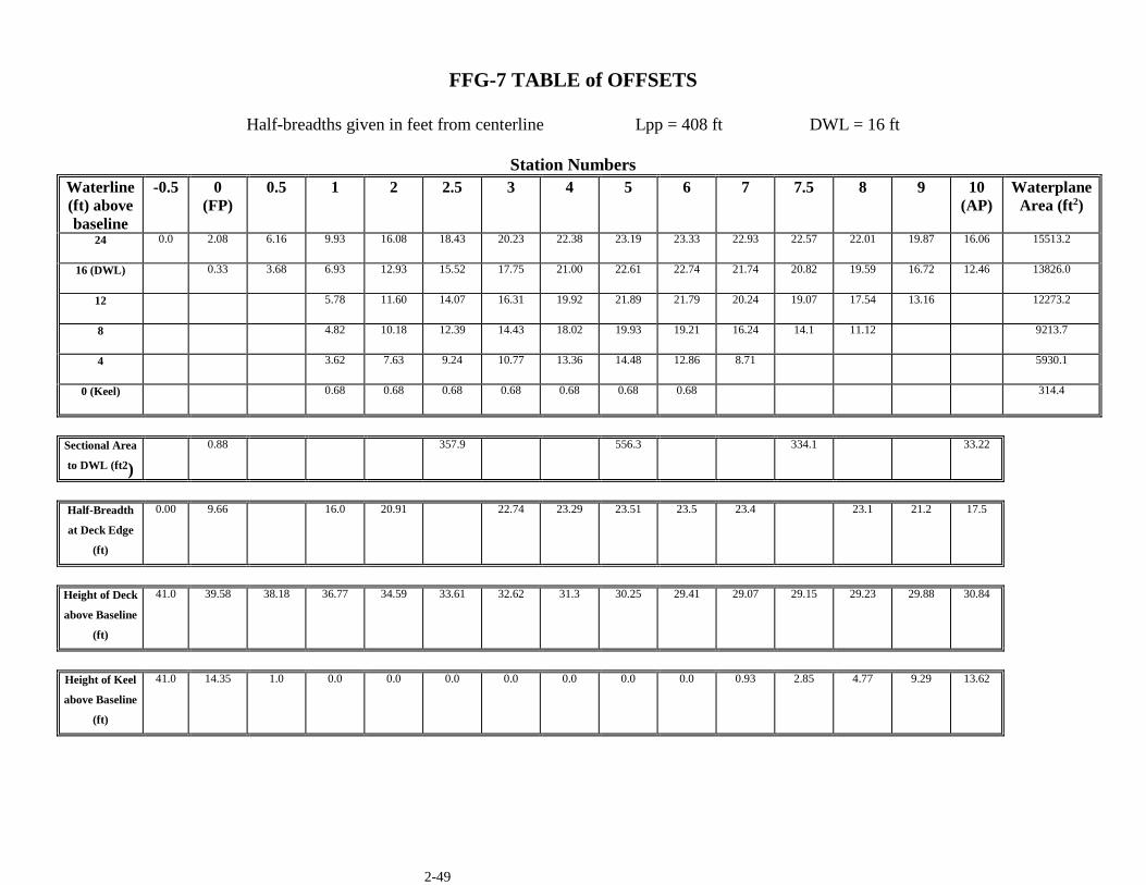
7. For this question, use a full sheet of graph paper for each drawing. Choose a scale that gives the best representation of the ship’s lines. Use the FFG-7 Table of Offsets given on the following page for your drawings.
a. For stations 0-10 draw a Body Plan for the ship up to the main deck. Omit stations
2.5 and 7.5.
b. Draw a half-breadth plan showing the 4 ft, 12 ft, 24 ft waterlines, and the deck edge.
c. Draw the sheer profile of the ship. Section 2.7 Center of Flotation & Center of Buoyancy 8. A box-shaped barge has the following dimensions: Length = 100 feet, Beam = 40 feet,
Depth = 25 feet. The barge is floating at a draft of 10 feet.
a. Draw a waterplane, profile, and end view of the barge. On each view indicate the following: centerline, waterline, midships, center of buoyancy (B), and center of flotation (F).
b. On your drawing show the following distances: KB, LCF referenced from the
forward perpendicular, and LCB referenced from amidships. c. Based on the given dimensions of the barge, determine the following dimensions: i. KB ii. LCF referenced to amidships iii. LCB referenced to the forward perpendicular iv. Height of F above the keel
2-49
FFG-7 TABLE of OFFSETS
Half-breadths given in feet from centerline Lpp = 408 ft DWL = 16 ft
Station Numbers Waterline (ft) above baseline
-0.5 0 (FP)
0.5 1 2 2.5 3 4 5 6 7 7.5 8 9 10 (AP)
Waterplane Area (ft2)
24 0.0 2.08 6.16 9.93 16.08 18.43 20.23 22.38 23.19 23.33 22.93 22.57 22.01 19.87 16.06 15513.2 16 (DWL) 0.33 3.68 6.93 12.93 15.52 17.75 21.00 22.61 22.74 21.74 20.82 19.59 16.72 12.46 13826.0
12 5.78 11.60 14.07 16.31 19.92 21.89 21.79 20.24 19.07 17.54 13.16 12273.2 8 4.82 10.18 12.39 14.43 18.02 19.93 19.21 16.24 14.1 11.12 9213.7 4 3.62 7.63 9.24 10.77 13.36 14.48 12.86 8.71 5930.1
0 (Keel) 0.68 0.68 0.68 0.68 0.68 0.68 0.68 314.4
Sectional Area
to DWL (ft2) 0.88 357.9 556.3 334.1 33.22
Half-Breadth
at Deck Edge
(ft)
0.00 9.66 16.0 20.91 22.74 23.29 23.51 23.5 23.4 23.1 21.2 17.5
Height of Deck
above Baseline
(ft)
41.0 39.58 38.18 36.77 34.59 33.61 32.62 31.3 30.25 29.41 29.07 29.15 29.23 29.88 30.84
Height of Keel
above Baseline
(ft)
41.0 14.35 1.0 0.0 0.0 0.0 0.0 0.0 0.0 0.0 0.93 2.85 4.77 9.29 13.62

2-50
Section 2.8 Simpson’s Rule For each Simpson’s Rule problem, show all solution steps in your work (i.e. diagram, differential element and its dimensions, labels, general calculus equation, general Simpson equation, numeric substitution, and final answer) 9. Using Simpson’s Rule calculate the areas of the following objects: a. Right triangle with base length of “a” and a height of length “b”. b. Semi-circle of radius “r”. c. Equilateral triangle with each side having length “a”. Section 2.9 Waterplane Area 10. The FFG-7 table of offsets gives waterplane areas calculated using all stations. Using
data for stations 0, 2.5, 5, 7.5, and 10, calculate the waterplane area at the DWL and compare your result with the given waterplane area.
11. Using the FFG-7 table of offsets, calculate the sectional area of station 3 up to the DWL. 12. Using the FFG-7 table of offsets, calculate the area of station 6 up to the 24 foot
waterline. 13. Using the sectional areas for stations 0, 2.5, 5, 7.5, and 10 calculate the following: a. Submerged volume of the FFG-7 up to the design waterline. b. Displacement in salt water. c. Displacement in fresh water. 14. Using the FFG-7 table of offsets, and stations 0, 2.5, 5, 7.5, and 10, calculate the location
of the longitudinal center of flotation (LCF) of the DWL referenced to amidships.

2-51
Section 2.10 Curves of Form 15. The Curves of Form for a ship are a graphical representation of its hydrostatic properties.
When computing a ship’s hydrostatic properties and creating the Curves of Form, what 2 assumptions are made?
16. An FFG-7 is floating on an even keel at a draft of 14 feet. Using its Curves of Form, find
the following parameters: a. Displacement (D) b. Longitudinal center of flotation (LCF) c. Vertical center of buoyancy (KB) d. Tons per inch immersion (TPI) e. Moment to trim 1 inch (MT1") f. Submerged volume 17. An FFG-7 is floating with a forward draft of 14.9 feet and an aft draft of 15.5 feet.
Determine the following: a. Displacement (D) b. Longitudinal center of flotation (LCF) c. Moment to trim 1 inch (MT1") 18. The FFG in problem 15 changes its draft from 14 feet to 15.5 feet. What is the new value
of TPI? Why does this value of TPI change? 19. A DDG-51 is floating on an even keel at a draft of 21.5 feet. A piece of machinery
weighing 150 LT is added to the ship. a. At which position on the ship must the weight be added so that trim does not
change? b. What is the change in ship’s draft, in feet, due to the weight addition? c. Compute the final draft after the weight addition. 20. A DDG-51 is floating on an even keel at a draft of 21.5 feet. A piece of machinery
weighing 50 LT is moved from the center of flotation to a point 150 feet forward of F. What is the change in ship’s trim due to this weight shift.