Embed Size (px)
Citation preview

A review of heterogeneous data mining for brain disorderidentification
Bokai Cao • Xiangnan Kong • Philip S. Yu
Received: 5 August 2015 /Accepted: 18 September 2015 / Published online: 30 September 2015
� The Author(s) 2015. This article is published with open access at Springerlink.com
Abstract With rapid advances in neuroimaging tech-
niques, the research on brain disorder identification has
become an emerging area in the data mining community.
Brain disorder data poses many unique challenges for data
mining research. For example, the raw data generated by
neuroimaging experiments is in tensor representations,
with typical characteristics of high dimensionality, struc-
tural complexity, and nonlinear separability. Furthermore,
brain connectivity networks can be constructed from the
tensor data, embedding subtle interactions between brain
regions. Other clinical measures are usually available
reflecting the disease status from different perspectives. It
is expected that integrating complementary information in
the tensor data and the brain network data, and incorpo-
rating other clinical parameters will be potentially trans-
formative for investigating disease mechanisms and for
informing therapeutic interventions. Many research efforts
have been devoted to this area. They have achieved great
success in various applications, such as tensor-based
modeling, subgraph pattern mining, and multi-view feature
analysis. In this paper, we review some recent data mining
methods that are used for analyzing brain disorders.
Keywords Data mining � Brain diseases � Tensoranalysis � Subgraph patterns � Feature selection
1 Introduction
Many brain disorders are characterized by ongoing injury
that is clinically silent for prolonged periods and irre-
versible by the time symptoms first present. New approa-
ches for detection of early changes in subclinical periods
will afford powerful tools for aiding clinical diagnosis,
clarifying underlying mechanisms, and informing neuro-
protective interventions to slow or reverse neural injury for
a broad spectrum of brain disorders, including bipolar
disorder, HIV infection on brain, Alzheimer’s disease,
Parkinson’s disease, etc. Early diagnosis has the potential
to greatly alleviate the burden of brain disorders and the
ever increasing costs to families and society.
As the identification of brain disorders is extremely
challenging, many different diagnosis tools and methods
have been developed to obtain a large number of mea-
surements from various examinations and laboratory tests.
Especially, recent advances in the neuroimaging technol-
ogy have provided an efficient and noninvasive way for
studying the structural and functional connectivity of the
human brain, either normal or in a diseased state [1]. This
can be attributed in part to advances in magnetic resonance
imaging (MRI) capabilities [2]. Techniques such as diffu-
sion MRI, also referred to as diffusion tensor imaging
(DTI), produce in vivo images of the diffusion process of
water molecules in biological tissues. By leveraging the
fact that the water molecule diffusion patterns reveal
B. Cao (&) � P. S. YuDepartment of Computer Science, University of Illinois at
Chicago, Chicago, IL 60607, USA
e-mail: [email protected]
X. Kong
Department of Computer Science, Worcester Polytechnic
Institute, Worcester, MA 01609, USA
e-mail: [email protected]
P. S. Yu
Institute for Data Science, Tsinghua University, Beijing, China
e-mail: [email protected]
123
Brain Informatics (2015) 2:253–264
DOI 10.1007/s40708-015-0021-3

microscopic details about tissue architecture, DTI can be
used to perform tractography within the white matter and
construct structural connectivity networks [3–7]. Func-
tional MRI (fMRI) is a functional neuroimaging procedure
that identifies localized patterns of brain activation by
detecting associated changes in the cerebral blood flow.
The primary form of fMRI uses the blood-oxygenation-
level-dependent (BOLD) response extracted from the gray
matter [8–10]. Another neuroimaging technique is positron
emission tomography (PET). Using different radioactive
tracers (e.g., fluorodeoxyglucose), PET produces a three-
dimensional image of various physiological, biochemical,
and metabolic processes [11].
A variety of data representations can be derived from
these neuroimaging experiments, which present many
unique challenges for the data mining community. Con-
ventional data mining algorithms are usually developed to
tackle data in one specific representation, a majority of
which are particularly for vector-based data. However, the
raw neuroimaging data are in the form of tensors, from
which we can further construct brain networks connecting
regions of interest (ROIs). Both of them are highly struc-
tured considering correlations between adjacent voxels in
the tensor data and that between connected brain regions in
the brain network data. Moreover, it is critical to explore
interactions between measurements computed from the
neuroimaging and other clinical experiments which
describe subjects in different vector spaces. In this paper,
we review some recent data mining methods for (1) mining
tensor imaging data; (2) mining brain networks; and (3)
mining multi-view feature vectors.
2 Tensor imaging analysis
For brain disorder identification, the raw data generated by
neuroimaging experiments are in tensor representations
[11–13]. For example, in contrast to two-dimensional
X-ray images, an fMRI sample corresponds to a four-di-
mensional array by recording the sequential changes of
traceable signals in each voxel.1
Tensors are higher order arrays that generalize the
concepts of vectors (first-order tensors) and matrices
(second-order tensors), whose elements are indexed by
more than two indices. Each index expresses a mode of
variation of the data and corresponds to a coordinate
direction. In an fMRI sample, the first three modes usually
encode the spatial information, while the fourth mode
encodes the temporal information. The number of variables
in each mode indicates the dimensionality of a mode. The
order of a tensor is determined by the number of its modes.
An mth-order tensor can be represented as
X ¼ ðxi1;...;imÞ 2 RI1�����Im , where Ii is the dimension of Xalong the i-th mode.
Definition 1 (Tensor product) The tensor product of
three vectors a 2 RI1 , b 2 RI2 ; and c 2 RI3 , denoted by
a� b� c, represents a third-order tensor with the elements
a� b� cð Þi1;i2;i3 ¼ ai1bi2ci3 .
Tensor product is also referred to as outer product in
some literature [11, 12]. An mth-order tensor is a rank-one
tensor if it can be defined as the tensor product of
m vectors.
Definition 2 Given a third-order tensor X 2 RI1�I2�I3 and
an integer R, as illustrated in Fig. 1, a tensor factorization
of X can be expressed as
X ¼ X 1 þ X 2 þ � � � þ XR ¼XR
r¼1
ar � br � cr ð1Þ
One of the major difficulties brought by the tensor data
is the curse of dimensionality. The total number of voxels
contained in a multi-mode tensor, say, X ¼ ðxi1;...;imÞ 2RI1�����Im is I1 � � � � � Im which is exponential to the
number of modes. If we unfold the tensor into a vector, the
number of features will be extremely high [14]. This makes
traditional data mining methods prone to overfitting,
especially with a small sample size. Both computational
scalability and theoretical guarantee of the traditional
models are compromised by such high dimensionality [13].
On the other hand, complex structural information is
embedded in the tensor data. For example, in the neu-
roimaging data, values of adjacent voxels are usually cor-
related with each other [2]. Such spatial relationships among
different voxels in a tensor image can be very important in
neuroimaging applications. Conventional tensor-based
approaches focus on reshaping the tensor data into matrices/
vectors, and thus, the original spatial relationships are lost.
The integration of structural information is expected to
improve the accuracy and interpretability of tensor models.
2.1 Supervised learning
Suppose we have a set of tensor data D ¼ fðX i; yiÞgni¼1 for
classification problem, where X i 2 RI1�����Im is the
Fig. 1 Tensor factorization of a third-order tensor
1 A voxel is the smallest three-dimensional point volume referenced
in a neuroimaging of the brain.
254 B. Cao et al.
123

neuroimaging data represented as an mth-order tensor and
yi 2 f�1;þ1g is the corresponding binary class label of
X i. For example, if the i-th subject has Alzheimer’s dis-
ease, the subject is associated with a positive label, i.e.,
yi ¼ þ1. Otherwise, if the subject is in the control group,
the subject is associated with a negative label, i.e., yi ¼ �1.
Supervised tensor learning can be formulated as the
optimization problem of support tensor machines (STMs)
[15] which is a generalization of the standard support vector
machines (SVMs) from vector data to tensor data. The
objective of such learning algorithms is to learn a hyperplane
by which the samples with different labels are divided as
wide as possible. However, tensor data may not be linearly
separable in the input space. To achieve a better performance
on finding the most discriminative biomarkers or identifying
infected subjects from the control group, in many neu-
roimaging applications, nonlinear transformation of the
original tensor data should be considered. He et al. study the
problem of supervised tensor learningwith nonlinear kernels
which can preserve the structure of tensor data [13]. The
proposed kernel is an extension of kernels in the vector space
to the tensor space which can take the multidimensional
structure complexity into account. However, it cannot
automatically consider the abundant and complicated
information of the neuroimaging data in an integral manner.
Han et al. apply a deep learning-based algorithm, the hier-
archical convolutional sparse auto-encoder, to extract effi-
cient and robust features and conserve abundant detail
information for the neuroimaging classification [16].
Slightly different from classifying disease status (dis-
crete label), another family of problems uses tensor neu-
roimages to predict cognitive outcome (continuous label).
The problems can be formulated in a regression setup by
treating clinical outcome as the real label, i.e., yi 2 R, and
treating tensor neuroimages as the input. However, most
classical regression methods take vectors as input features.
Simply reshaping a tensor into a vector is clearly an
unsatisfactory solution.
Zhou et al. exploit the tensor structure in imaging data and
integrate tensor decomposition within a statistical regression
paradigm to model multidimensional arrays [14]. By
imposing a low-rank approximation to the extremely high-
dimensional complex imaging data, the curse of dimen-
sionality is greatly alleviated, thereby allowing development
of a fast estimation algorithm and regularization. Numerical
analysis demonstrates its potential applications in identify-
ing ROI in brains that are relevant to a particular clinical
response. In scenarios where the objective is to predict a set
of dependent variables, Cichocki et al. introduce a general-
ized multilinear regression model, higher order partial least
squares, which projects the electrocorticogram data into a
latent space and performs regression on the corresponding
latent variables [17, 18].
2.2 Unsupervised learning
Modern imaging techniques have allowed us to study the
human brain as a complex system by modeling it as a net-
work [19]. For example, the fMRI scans consist of activa-
tions of thousands of voxels over time embedding a complex
interaction of signals and noise [20], which naturally pre-
sents the problem of eliciting the underlying network from
brain activities in the spatio-temporal tensor data. A brain
connectivity network, also called a connectome [21], con-
sists of nodes (gray matter regions) and edges (white matter
tracts in structural networks or correlations between two
BOLD time series in functional networks).
Although the anatomical atlases in the brain have been
extensively studied for decades, task/subject specific net-
works have still not been completely explored with con-
sideration of functional or structural connectivity
information. An anatomically parcellated region may
contain subregions that are characterized by dramatically
different functional or structural connectivity patterns,
thereby significantly limiting the utility of the constructed
networks. There are usually trade-offs between reducing
noise and preserving utility in brain parcellation [2]. Thus,
investigating how to directly construct brain networks from
tensor imaging data and understanding how they develop,
deteriorate, and vary across individuals will benefit disease
diagnosis [12].
Davidson et al. pose the problem of network discovery
from fMRI data which involves simplifying spatio-tem-
poral data into regions of the brain (nodes) and relation-
ships between those regions (edges) [12]. Here the nodes
represent collections of voxels that are known to behave
cohesively over time; the edges can indicate a number of
properties between nodes such as facilitation/inhibition
(increases/decreases activity) or probabilistic (synchro-
nized activity) relationships; and the weight associated
with each edge encodes the strength of the relationship.
A tensor can be decomposed into several factors.
However, unconstrained tensor decomposition results of
the fMRI data may not be good for node discovery because
each factor is typically not a spatially contiguous region
nor does it necessarily match an anatomical region. That is
to say, many spatially adjacent voxels in the same structure
are not active in the same factor which is anatomically
impossible. Therefore, to achieve the purpose of discov-
ering nodes while preserving anatomical adjacency, known
anatomical regions in the brain are used as masks and
constraints are added to enforce that the discovered factors
should closely match these masks [12].
Yang et al. investigate the inference of mouse brain
networks and propose a hierarchical graphical model
framework with tree-structural regularization [22]. In the
hierarchical structure, voxels serve as the leaf nodes of the
A review of heterogeneous data mining for brain disorder identification 255
123

tree, and a node in the intermediate layer represents a
region formed by voxels in the subtree rooted at that node.
For edge discovery problem, Papalexakis et al. leverage
control theory to model the dynamics of neuron interac-
tions and infer the functional connectivity [23]. It is
assumed that in addition to the linear influence of the input
stimulus, there are hidden neuron regions of the brain,
which interact with each other, causing the voxel activities.
Veeriah et al. propose a deep learning algorithm for pre-
dicting if the two brain neurons are causally connected
given their activation time-series data [24]. It reveals that
the exploitation of the deep architecture is critical, which
jointly extracts sequences of salient patterns of activation
and aligns them to predict neural connections.
Overall, current research on tensor imaging analysis
presents two directions: (1) supervised: for a particular
brain disorder, a classifier can be trained by modeling the
relationship between a set of neuroimages and their asso-
ciated labels (disease status or clinical response); (2)
unsupervised: regardless of brain disorders, a brain net-
work can be discovered from a given neuroimage.
3 Brain network analysis
We have briefly introduced that brain networks can be
constructed from neuroimaging data where nodes corre-
spond to brain regions, e.g., insula, hippocampus, thala-
mus, and links correspond to the functional/structural
connectivity between brain regions. The linkage structure
in brain networks can encode tremendous information
about the mental health of human subjects. For example, in
brain networks derived from fMRI, functional connections
can encode the correlations between the functional activi-
ties of brain regions. While structural links in DTI brain
networks can capture the number of neural fibers con-
necting different brain regions. The complex structures and
the lack of vector representations for the brain network data
raise major challenges for data mining.
Next, we will discuss different approaches on how to
conduct further analysis for constructed brain networks,
which are also referred to as graphs hereafter.
Definition 3 (Binary graph) A binary graph is repre-
sented as G ¼ ðV ;EÞ, where V ¼ fv1; . . .; vnvg is the set of
vertices, and E � V � V is the set of deterministic edges.
3.1 Kernel learning on graphs
In the setting of supervised learning on graphs, the target is
to train a classifier using a given set of graph data
D ¼ fðGi; yiÞgni¼1, so that we can predict the label y for a
test graph G. With applications to brain networks, it is
desirable to identify the disease status for a subject based
on his/her uncovered brain network. Recent development
of brain network analysis has made characterization of
brain disorders at a whole-brain connectivity level possible,
thus providing a new direction for brain disease
classification.
Due to the complex structures and the lack of vector
representations, graph data cannot be directly used as the
input for most data mining algorithms. A straightforward
solution that has been extensively explored is to first derive
features from brain networks and then construct a kernel on
the feature vectors.
Wee et al. use brain connectivity networks for disease
diagnosis on mild cognitive impairment (MCI), which is
an early phase of Alzheimer’s disease (AD) and usually
regarded as a good target for early diagnosis and thera-
peutic interventions [25–27]. In the step of feature
extraction, weighted local clustering coefficients of each
ROI in relation to the remaining ROIs are extracted from
all the constructed brain networks to quantify the preva-
lence of clustered connectivity around the ROIs. To select
the most discriminative features for classification, statis-
tical t test is performed and features with p values smaller
than a predefined threshold are selected to construct a
kernel matrix. Through the employment of the multi-
kernel SVM, Wee et al. integrate information from DTI
and fMRI and achieve accurate early detection of brain
abnormalities [27].
However, such strategy simply treats a graph as a col-
lection of nodes/links, and then extracts local measures
(e.g., clustering coefficient) for each node or performs
statistical analysis on each link, thereby blinding the con-
nectivity structures of brain networks. Motivated by the
fact that some data in real-world applications are naturally
represented by means of graphs, while compressing and
converting them to vectorial representations would defi-
nitely lose structural information, kernel methods for
graphs have been extensively studied for a decade [28].
A graph kernel maps the graph data from the original
graph space to the feature space and further measures the
similarity between two graphs by comparing their topo-
logical structures [29]. For example, product graph kernel
is based on the idea of counting the number of walks in
product graphs [30]; marginalized graph kernel works by
comparing the label sequences generated by synchronized
random walks of labeled graphs [31]; and cyclic pattern
kernels for graphs count pairs of matching cyclic/tree
patterns in two graphs [32].
To identify individuals with AD/MCI from healthy
controls, instead of using only a single property of brain
networks, Jie et al. integrate multiple properties of fMRI
brain networks to improve the disease diagnosis perfor-
mance [33]. Two different yet complementary network
256 B. Cao et al.
123

properties, i.e., local connectivity and global topological
properties are quantified by computing two different types
of kernels, i.e., a vector-based kernel and a graph kernel.
As a local network property, weighted clustering coeffi-
cients are extracted to compute a vector-based kernel. As a
topology-based graph kernel, Weisfeiler-Lehman subtree
kernel [29] is used to measure the topological similarity
between paired fMRI brain networks. It is shown that this
type of graph kernel can effectively capture the topological
information from fMRI brain networks. The multi-kernel
SVM is employed to fuse these two heterogeneous kernels
for distinguishing individuals with MCI from healthy
controls.
3.2 Subgraph pattern mining
In brain network analysis, the ideal patterns we want to
mine from the data should take care of both local and
global graph topological information. Graph kernel meth-
ods seem promising, which, however, are not interpretable.
Subgraph patterns are more suitable for brain networks,
which can simultaneously model the network connectivity
patterns around the nodes and capture the changes in local
area [2].
Definition 4 (Subgraph) Let G0 ¼ ðV 0;E0Þ and G ¼ðV;EÞ be two binary graphs. G0 is a subgraph of G (denoted
as G0 � G) iff V 0 � V and E0 � E. If G0 is a subgraph of G,
then G is supergraph of G0.
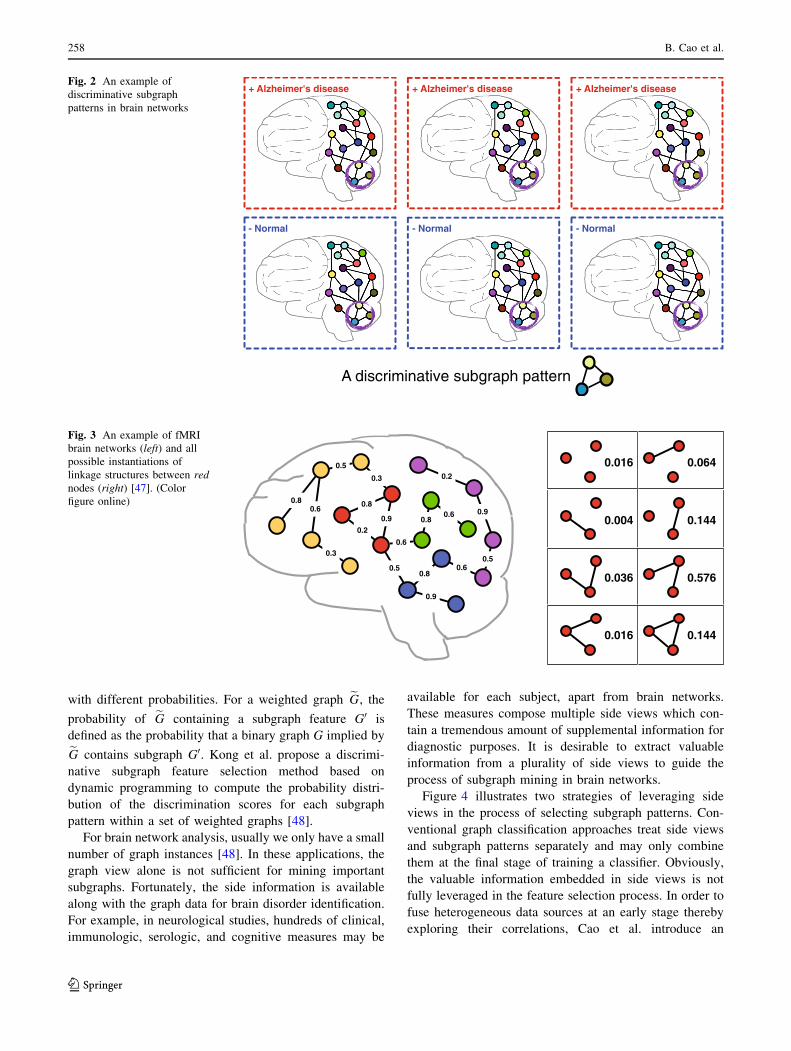
A subgraph pattern, in a brain network, represents a
collection of brain regions and their connections. For
example, as shown in Fig. 2, three brain regions should
work collaboratively for normal people and the absence of
any connection between them can result in Alzheimer’s
disease in different degrees. Therefore, it is valuable to
understand which connections collectively play a signifi-
cant role in disease mechanism by finding discriminative
subgraph patterns in brain networks.
Mining subgraph patterns from graph data has been
extensively studied by many researchers [34–37]. In gen-
eral, a variety of filtering criteria are proposed. A typical
evaluation criterion is frequency, which aims at searching
for frequently appearing subgraph features in a graph
dataset satisfying a prespecified threshold. Most of the
frequent subgraph mining approaches are unsupervised.
For example, Yan and Han develop a depth-first search
algorithm: gSpan [38]. This algorithm builds a lexico-
graphic order among graphs, and maps each graph to a
unique minimum DFS code as its canonical label. Based on
this lexicographic order, gSpan adopts the depth-first
search strategy to mine frequent connected subgraphs
efficiently. Many other approaches for frequent subgraph
mining have also been proposed, e.g., AGM [39], FSG
[40], MoFa [41], FFSM [42], and Gaston [43].
Moreover, the problem of supervised subgraph mining
has been studied in recent work which examines how to
improve the efficiency of searching the discriminative
subgraph patterns for graph classification. Yan et al.
introduce two concepts structural leap search and fre-
quency-descending mining, and propose LEAP [37] which
is one of the first work in discriminative subgraph mining.
Thoma et al. propose CORK which can yield a near-opti-
mal solution using greedy feature selection [36]. Ranu and
Singh propose a scalable approach, called GraphSig, that is
capable of mining discriminative subgraphs with a low-
frequency threshold [44]. Jin et al. propose COM which
takes into account the co-occurrences of subgraph patterns,
thereby facilitating the mining process [45]. Jin et al. fur-
ther propose an evolutionary computation method, called
GAIA, to mine discriminative subgraph patterns using a
randomized searching strategy [34]. Zhu et al. design a
diversified discrimination score based on the log ratio
which can reduce the overlap between selected features by
considering the embedding overlaps in the graphs [46].
Conventional graph mining approaches are best suited
for binary edges, where the structure of graph objects is
deterministic, and the binary edges represent the presence
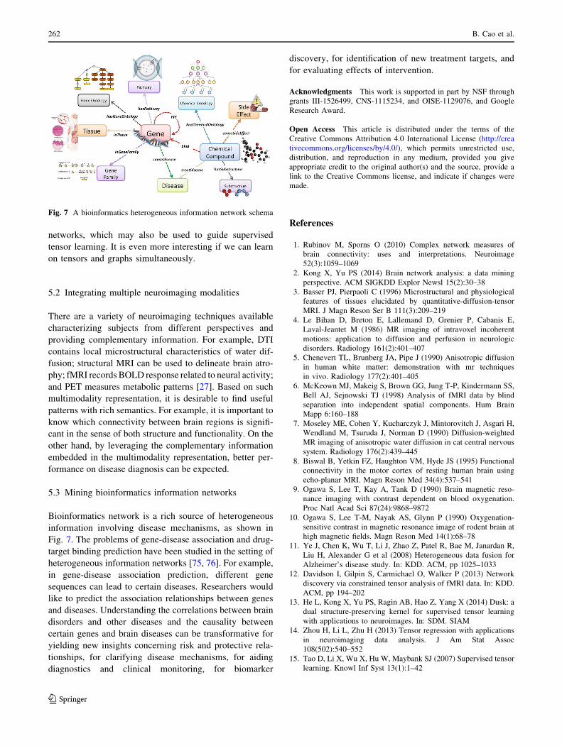
of linkages between the nodes [2]. In fMRI brain network
data, however, there are inherently weighted edges in the
graph linkage structure, as shown in Fig. 3 (left). A
straightforward solution is to threshold weighted networks
to yield binary networks. However, such simplification will
result in great loss of information. Ideal data mining
methods for brain network analysis should be able to
overcome these methodological problems by generalizing
the network edges to positive and negative weighted cases,
e.g., probabilistic weights in fMRI brain networks and
integral weights in DTI brain networks.
Definition 5 A weighted graph is represented as
eG ¼ ðV ;E; pÞ, where V ¼ fv1; . . .; vnvg is the set of ver-
tices, and E � V � V is the set of nondeterministic edges.
p : E ! ð0; 1� is a function that assigns a probability of
existence to each edge in E.
fMRI brain networks can be modeled as weighted
graphs where each edge e 2 E is associated with a prob-
ability p(e) indicating the likelihood of whether this edge
should exist or not [47, 48]. It is assumed that p(e) of
different edges in a weighted graph are independent from
each other. Therefore, by enumerating the possible exis-
tence of all edges in a weighted graph, we can obtain a set
of binary graphs. For example, in Fig. 3 (right), consider
the three red nodes and links between them as a weighted
graph. There are 23 ¼ 8 binary graphs that can be implied
A review of heterogeneous data mining for brain disorder identification 257
123
with different probabilities. For a weighted graph eG, the
probability of eG containing a subgraph feature G0 is
defined as the probability that a binary graph G implied by
eG contains subgraph G0. Kong et al. propose a discrimi-
native subgraph feature selection method based on
dynamic programming to compute the probability distri-
bution of the discrimination scores for each subgraph
pattern within a set of weighted graphs [48].
For brain network analysis, usually we only have a small
number of graph instances [48]. In these applications, the
graph view alone is not sufficient for mining important
subgraphs. Fortunately, the side information is available
along with the graph data for brain disorder identification.
For example, in neurological studies, hundreds of clinical,
immunologic, serologic, and cognitive measures may be
available for each subject, apart from brain networks.
These measures compose multiple side views which con-
tain a tremendous amount of supplemental information for
diagnostic purposes. It is desirable to extract valuable
information from a plurality of side views to guide the
process of subgraph mining in brain networks.
Figure 4 illustrates two strategies of leveraging side
views in the process of selecting subgraph patterns. Con-
ventional graph classification approaches treat side views
and subgraph patterns separately and may only combine
them at the final stage of training a classifier. Obviously,
the valuable information embedded in side views is not
fully leveraged in the feature selection process. In order to
fuse heterogeneous data sources at an early stage thereby
exploring their correlations, Cao et al. introduce an
+ Alzheimer's disease + Alzheimer's disease + Alzheimer's disease
- Normal - Normal - Normal
A discriminative subgraph pattern
Fig. 2 An example of
discriminative subgraph
patterns in brain networks
0.80.6
0.3
0.2
0.5
0.3
0.8
0.9
0.2
0.9
0.5
0.60.8
0.5
0.6
0.8
0.9
0.6
0.016
0.004
0.036
0.016
0.064
0.144
0.576
0.144
Fig. 3 An example of fMRI
brain networks (left) and all
possible instantiations of
linkage structures between red
nodes (right) [47]. (Color
figure online)
258 B. Cao et al.
123

effective algorithm for discriminative subgraph selection
using multiple side views as guidance [49]. Side informa-
tion consistency is first validated via statistical hypothesis
testing which suggests that the similarity of side view
features between instances with the same label should have
higher probability to be larger than that with different
labels. Based on such observations, it is assumed that the
similarity/distance between instances in the space of sub-
graph features should be consistent with that in the space of
a side view. That is to say, if two instances are similar in
the space of a side view, they should also be close to each
other in the space of subgraph features. Therefore the target
is to minimize the distance between subgraph features of
each pair of similar instances in each side view [49]. In
contrast to existing subgraph mining approaches that focus
on the graph view alone, the proposed method can explore
multiple vector-based side views to find an optimal set of
subgraph features for graph classification.
For graph classification, brain network analysis
approaches can generally be put into three groups: (1)
extracting some local measures (e.g., clustering coefficient)
to train a standard vector-based classifier; (2) directly
adopting graph kernels for classification; and (3) finding
discriminative subgraph patterns. Different types of meth-
ods model the connectivity embedded in brain networks in
different ways.
4 Multi-view feature analysis
Medical science witnesses everyday measurements from a
series of medical examinations documented for each sub-
ject, including clinical, imaging, immunologic, serologic,
and cognitive measures [50], as shown in Fig. 5. Each
group of measures characterizes the health state of a sub-
ject from different aspects. This type of data is named as
multi-view data, and each group of measures form a dis-
tinct view quantifying subjects in one specific feature
space. Therefore, it is critical to combine them to improve
the learning performance, while simply concatenating
features from all views and transforming a multi-view data
into a single-view data, as the method (a) shown in Fig. 6,
would fail to leverage the underlying correlations between
different views.
4.1 Multi-view learning and feature selection
Suppose we have a multi-view classification task with n
labeled instances represented from m different views:
D ¼ xð1Þi ; x
ð2Þi ; . . .; x
ðmÞi ; yi
� �n on
i¼1, where x
ðvÞi 2 RIv , Iv is
the dimensionality of the v-th view, and yi 2 f�1;þ1g is
the class label of the i-th instance.
Representative methods for multi-view learning can be
categorized into three groups: co-training, multiple kernel
learning, and subspace learning [52]. Generally, the co-
training style algorithm is a classic approach for semi-su-
pervised learning, which trains in alternation to maximize
the mutual agreement on different views. Multiple kernel
learning algorithms combine kernels that naturally corre-
spond to different views, either linearly [53] or nonlinearly
[54, 55] to improve learning performance. Subspace
learning algorithms learn a latent subspace, from which
multiple views are generated. Multiple kernel learning and
subspace learning are generalized as co-regularization style
algorithms [56], where the disagreement between the
functions of different views is taken as a part of the
objective function to be minimized. Overall, by exploring
the consistency and complementary properties of different
views, multi-view learning is more effective than single-
view learning.
In the multi-view setting for brain disorders, or for
medical studies in general, a critical problem is that there
may be limited subjects available (i.e., a small n) yet
introducing a large number of measurements (i.e., a largePmi¼1 Ii). Within the multi-view data, not all features in
different views are relevant to the learning task, and some
irrelevant features may introduce unexpected noise. The
irrelevant information can even be exaggerated after view
combinations thereby degrading performance. Therefore, it
is necessary to take care of feature selection in the learning
process. Feature selection results can also be used by
researchers to find biomarkers for brain diseases. Such
biomarkers are clinically imperative for detecting injury to
the brain in the earliest stage before it is irreversible. Valid
biomarkers can be used to aid diagnosis, monitor disease
progression, and evaluate effects of intervention [48].
Conventional feature selection approaches can be divi-
ded into three main directions: filter, wrapper, and
Subgraph Patterns
Side Views
Mine
noisuFetaLnoisuFylraE
Brain Networks Graph ClassificationInput
Fig. 4 Two strategies of
leveraging side views in feature
selection process for graph
classification: late fusion and
early fusion
A review of heterogeneous data mining for brain disorder identification 259
123

embedded methods [57]. Filter methods compute a dis-
crimination score of each feature independently of the
other features based on the correlation between the feature
and the label, e.g., information gain, Gini index, Relief [58,
59]. Wrapper methods measure the usefulness of feature
subsets according to their predictive power, optimizing the
subsequent induction procedure that uses the respective
subset for classification [51, 60–63]. Embedded methods
perform feature selection in the process of model training
based on sparsity regularization [64–67]. For example,
Miranda et al. add a regularization term that penalizes the
size of the selected feature subset to the standard cost
function of SVM, thereby optimizing the new objective
function to conduct feature selection [68]. Essentially, the
process of feature selection and learning algorithm interact
in embedded methods which means the learning part and
the feature selection part cannot be separated, while
wrapper methods utilize the learning algorithm as a black
box.
However, directly applying these feature selection
approaches to each separate view would fail to leverage
multi-view correlations. By taking into account the latent
interactions among views and the redundancy triggered by
multiple views, it is desirable to combine multi-view data
in a principled manner and perform feature selection to
obtain consensus and discriminative low-dimensional fea-
ture representations.
4.2 Modeling view correlations
Recent years have witnessed many research efforts devoted
to the integration of feature selection and multi-view
learning. Tang et al. study multi-view feature selection in
the unsupervised setting by constraining that similar data
instances from each view should have similar pseudo-class
labels [69]. Considering brain disorder identification, dif-
ferent neuroimaging features may capture different but
complementary characteristics of the data. For example,
the voxel-based tensor features convey the global infor-
mation, while the ROI-based automated anatomical label-
ing (AAL) [70] features summarize the local information
from multiple representative brain regions. Incorporating
these data and additional nonimaging data sources can
potentially improve the prediction. For Alzheimer’s disease
(AD) classification, Ye et al. propose a kernel-based
method for integrating heterogeneous data, including ten-
sor and AAL features from MRI images, demographic
information, and genetic information [11]. The kernel
framework is further extended for selecting features
(biomarkers) from heterogeneous data sources that play
more significant roles than others in AD diagnosis.
Huang et al. propose a sparse composite linear dis-
criminant analysis model for identification of disease-re-
lated brain regions of AD from multiple data sources [71].
Two sets of parameters are learned: one represents the
common information shared by all the data sources about a
feature, and the other represents the specific information
only captured by a particular data source about the feature.
Experiments are conducted on the PET and MRI data
which measure structural and functional aspects, respec-
tively, of the same AD pathology. However, the proposed
approach requires the input as the same set of variables
from multiple data sources. Xiang et al. investigate multi-
source incomplete data for AD and introduce a unified
feature learning model to handle block-wise missing data
which achieves simultaneous feature-level and source-level
selection [72].
For modeling view correlations, in general, a coefficient
is assigned for each view, either at the view-level or
HIV/seronega�ve
View 1
View 3
View 2
View 6
View 4
View 5
Immunologic measures
Clinical measuresSerologic measures
MRI sequence B
MRI sequence A Cogni�ve measures
Fig. 5 An example of multi-view learning in medical studies [51]
View 3
View 2
View 1
Modeling Feature selec�on
Method (a)
Method (b)
Method (c)
Fig. 6 Schematic view of the key differences among three strategies
of multi-view feature selection [51]
260 B. Cao et al.
123

feature-level. For example, in multiple kernel learning, a
kernel is constructed from each view and a set of kernel
coefficients are learned to obtain an optimal combined
kernel matrix. These approaches, however, fail to explicitly
consider correlations between features.
4.3 Modeling feature correlations
One of the key issues for multi-view classification is to
choose an appropriate tool to model features and their
correlations hidden in multiple views, since this directly
determines how information will be used. In contrast to
modeling on views, another direction for modeling multi-
view data is to directly consider the correlations between
features from multiple views. Since taking the tensor pro-
duct of their respective feature spaces corresponds to the
interaction of features from multiple views, the concept of
tensor serves as a backbone for incorporating multi-view
features into a consensus representation by means of tensor
product, where the complex multiple relationships among
views are embedded within the tensor structures. By min-
ing structural information contained in the tensor, knowl-
edge of multi-view features can be extracted and used to
establish a predictive model.
Smalter et al. formulate the problem of feature selection
in the tensor product space as an integer quadratic pro-
gramming problem [73]. However, this method is compu-
tationally intractable on many views, since it directly selects
features in the tensor product space resulting in the curse of
dimensionality, as the method (b) shown in Fig. 6. Cao et al.
propose to use a tensor-based approach tomodel features and
their correlations hidden in the original multi-view data [51].
The operation of tensor product can be used to bringm-view
feature vectors of each instance together, leading to a ten-
sorial representation for common structure across multiple
views, and allowing us to adequately diffuse relationships
and encode information among multi-view features. In this
manner, the multi-view classification task is essentially
transformed from an independent domain of each view to a
consensus domain as a tensor classification problem.
By using X i to denoteQm
v¼1 �xðvÞi , the dataset of labeled
multi-view instances can be represented as
D ¼ fðX i; yiÞgni¼1. Note that each multi-view instance X i is
an mth-order tensor that lies in the tensor product space
RI1�����Im . Based on the definitions of inner product and
tensor norm, multi-view classification can be formulated as
a global convex optimization problem in the framework of
supervised tensor learning [15]. This model is named as
multi-view SVM [51], and it can be solved with the use of
optimization techniques developed for SVM.
Furthermore, a dual method for multi-view feature
selection is proposed in [51] that leverages the relationship
between original multi-view features and reconstructed
tensor product features to facilitate the implementation of
feature selection, as the method (c) in Fig. 6. It is a wrapper
model which selects useful features in conjunction with the
classifier and simultaneously exploits the correlations
among multiple views. Following the idea of SVM-based
recursive feature elimination [60], multi-view feature
selection is consistently formulated and implemented in the
framework of multi-view SVM. This idea can extend to
include lower order feature interactions and to employ a
variety of loss functions for classification or regression
[74].
5 Future work
The human brain is one of the most complicated biological
structures in the known universe. While it is very chal-
lenging to understand how it works, especially when dis-
orders and diseases occur, dozens of leading technology
firms, academic institutions, scientists, and other key con-
tributors to the field of neuroscience have devoted them-
selves to this area and made significant improvements in
various dimensions.2 Data mining on brain disorder iden-
tification has become an emerging area and a promising
research direction.
This paper provides an overview of data mining
approaches with applications to brain disorder identifica-
tion, which have attracted increasing attention in both data
mining and neuroscience communities in recent years. A
taxonomy is built based upon data representations, i.e.,
tensor imaging data, brain network data, and multi-view
data, following which the relationships between different
data mining algorithms and different neuroimaging appli-
cations are summarized. We briefly present some potential
topics of interest in the future.
5.1 Bridging heterogeneous data representations
As introduced in this paper, we can usually derive data
from neuroimaging experiments in three representations,
including raw tensor imaging data, brain network data, and
multi-view vector-based data. It is critical to study how to
train a model on a mixture of data representations, although
it is very challenging to combine data that are represented
in tensor space, vector space, and graph space, respec-
tively. There is a straightforward idea of defining different
kernels on different feature spaces and combing them
through multi-kernel algorithms. However, it is usually
hard to interpret the results. The concept of side view has
been introduced to facilitate the process of mining brain
2 http://www.whitehouse.gov/BRAIN
A review of heterogeneous data mining for brain disorder identification 261
123
networks, which may also be used to guide supervised
tensor learning. It is even more interesting if we can learn
on tensors and graphs simultaneously.
5.2 Integrating multiple neuroimaging modalities
There are a variety of neuroimaging techniques available
characterizing subjects from different perspectives and
providing complementary information. For example, DTI
contains local microstructural characteristics of water dif-
fusion; structural MRI can be used to delineate brain atro-
phy; fMRI records BOLD response related to neural activity;
and PET measures metabolic patterns [27]. Based on such
multimodality representation, it is desirable to find useful
patterns with rich semantics. For example, it is important to
know which connectivity between brain regions is signifi-
cant in the sense of both structure and functionality. On the
other hand, by leveraging the complementary information
embedded in the multimodality representation, better per-
formance on disease diagnosis can be expected.
5.3 Mining bioinformatics information networks
Bioinformatics network is a rich source of heterogeneous
information involving disease mechanisms, as shown in
Fig. 7. The problems of gene-disease association and drug-
target binding prediction have been studied in the setting of
heterogeneous information networks [75, 76]. For example,
in gene-disease association prediction, different gene
sequences can lead to certain diseases. Researchers would
like to predict the association relationships between genes
and diseases. Understanding the correlations between brain
disorders and other diseases and the causality between
certain genes and brain diseases can be transformative for
yielding new insights concerning risk and protective rela-
tionships, for clarifying disease mechanisms, for aiding
diagnostics and clinical monitoring, for biomarker
discovery, for identification of new treatment targets, and
for evaluating effects of intervention.
Acknowledgments This work is supported in part by NSF through
grants III-1526499, CNS-1115234, and OISE-1129076, and Google
Research Award.
Open Access This article is distributed under the terms of the
Creative Commons Attribution 4.0 International License (http://crea
tivecommons.org/licenses/by/4.0/), which permits unrestricted use,
distribution, and reproduction in any medium, provided you give
appropriate credit to the original author(s) and the source, provide a
link to the Creative Commons license, and indicate if changes were
made.
References
1. Rubinov M, Sporns O (2010) Complex network measures of
brain connectivity: uses and interpretations. Neuroimage
52(3):1059–1069
2. Kong X, Yu PS (2014) Brain network analysis: a data mining
perspective. ACM SIGKDD Explor Newsl 15(2):30–38
3. Basser PJ, Pierpaoli C (1996) Microstructural and physiological
features of tissues elucidated by quantitative-diffusion-tensor
MRI. J Magn Reson Ser B 111(3):209–219
4. Le Bihan D, Breton E, Lallemand D, Grenier P, Cabanis E,
Laval-Jeantet M (1986) MR imaging of intravoxel incoherent
motions: application to diffusion and perfusion in neurologic
disorders. Radiology 161(2):401–407
5. Chenevert TL, Brunberg JA, Pipe J (1990) Anisotropic diffusion
in human white matter: demonstration with mr techniques
in vivo. Radiology 177(2):401–405
6. McKeown MJ, Makeig S, Brown GG, Jung T-P, Kindermann SS,
Bell AJ, Sejnowski TJ (1998) Analysis of fMRI data by blind
separation into independent spatial components. Hum Brain
Mapp 6:160–188
7. Moseley ME, Cohen Y, Kucharczyk J, Mintorovitch J, Asgari H,
Wendland M, Tsuruda J, Norman D (1990) Diffusion-weighted
MR imaging of anisotropic water diffusion in cat central nervous
system. Radiology 176(2):439–445
8. Biswal B, Yetkin FZ, Haughton VM, Hyde JS (1995) Functional
connectivity in the motor cortex of resting human brain using
echo-planar MRI. Magn Reson Med 34(4):537–541
9. Ogawa S, Lee T, Kay A, Tank D (1990) Brain magnetic reso-
nance imaging with contrast dependent on blood oxygenation.
Proc Natl Acad Sci 87(24):9868–9872
10. Ogawa S, Lee T-M, Nayak AS, Glynn P (1990) Oxygenation-
sensitive contrast in magnetic resonance image of rodent brain at
high magnetic fields. Magn Reson Med 14(1):68–78
11. Ye J, Chen K, Wu T, Li J, Zhao Z, Patel R, Bae M, Janardan R,
Liu H, Alexander G et al (2008) Heterogeneous data fusion for
Alzheimer’s disease study. In: KDD. ACM, pp 1025–1033
12. Davidson I, Gilpin S, Carmichael O, Walker P (2013) Network
discovery via constrained tensor analysis of fMRI data. In: KDD.
ACM, pp 194–202
13. He L, Kong X, Yu PS, Ragin AB, Hao Z, Yang X (2014) Dusk: a
dual structure-preserving kernel for supervised tensor learning
with applications to neuroimages. In: SDM. SIAM
14. Zhou H, Li L, Zhu H (2013) Tensor regression with applications
in neuroimaging data analysis. J Am Stat Assoc
108(502):540–552
15. Tao D, Li X, Wu X, Hu W, Maybank SJ (2007) Supervised tensor
learning. Knowl Inf Syst 13(1):1–42
Fig. 7 A bioinformatics heterogeneous information network schema
262 B. Cao et al.
123

16. Han X, Zhong Y, He L, Philip SY, Zhang L (2015) The unsu-
pervised hierarchical convolutional sparse auto-encoder for neu-
roimaging data classification. In: Brain informatics and health.
Springer, pp 156–166
17. Cichocki A, Mandic D, De Lathauwer L, Zhou G, Zhao Q, Caiafa
C, Phan HA (2015) Tensor decompositions for signal processing
applications: from two-way to multiway component analysis.
Signal Process Mag 32(2):145–163
18. Zhao Q, Caiafa CF, Mandic DP, Chao ZC, Nagasaka Y, Fujii N,
Zhang L, Cichocki A (2013) Higher order partial least squares
(HOPLS): a generalized multilinear regression method. Pattern
Anal Mach Intell 35(7):1660–1673
19. Ajilore O, Zhan L, GadElkarim J, Zhang A, Feusner JD, Yang S,
Thompson PM, Kumar A, Leow A (2013) Constructing the
resting state structural connectome. Front Neuroinform 7:30
20. Genovese CR, Lazar NA, Nichols T (2002) Thresholding of
statistical maps in functional neuroimaging using the false dis-
covery rate. Neuroimage 15(4):870–878
21. Sporns O, Tononi G, Kotter R (2005) The human connectome: a
structural description of the human brain. PLoS Comput Biol
1(4):e42
22. Yang S, Sun Q, Ji S, Wonka P, Davidson I, Ye J (2015) Structural
graphical lasso for learning mouse brain connectivity. In: KDD.
ACM, pp 1385–1394
23. Papalexakis EE, Fyshe A, Sidiropoulos ND, Talukdar PP,
Mitchell TM, Faloutsos C (2014) Good-enough brain model:
challenges, algorithms and discoveries in multi-subject experi-
ments. In: KDD. ACM, pp 95–104
24. Veeriah V, Durvasula R, Qi GJ (2015) Deep learning architecture
with dynamically programmed layers for brain connectome pre-
diction. In: KDD. ACM, pp 1205–1214
25. Wee C-Y, Yap P-T, Denny K, Browndyke JN, Potter GG, Welsh-
Bohmer KA, Wang L, Shen D (2012) Resting-state multi-spec-
trum functional connectivity networks for identification of mci
patients. PloS One 7(5):e37828
26. Wee C-Y, Yap P-T, Li W, Denny K, Browndyke JN, Potter GG,
Welsh-Bohmer KA, Wang L, Shen D (2011) Enriched white
matter connectivity networks for accurate identification of mci
patients. Neuroimage 54(3):1812–1822
27. Wee C-Y, Yap P-T, Zhang D, Denny K, Browndyke JN, Potter
GG, Welsh-Bohmer KA, Wang L, Shen D (2012) Identification
of mci individuals using structural and functional connectivity
networks. Neuroimage 59(3):2045–2056
28. Camastra F, Petrosino A (2008) Kernel methods for graphs: a
comprehensive approach. In: Knowledge-based intelligent infor-
mation and engineering systems. Springer, pp 662–669
29. Shervashidze N, Schweitzer P, Van Leeuwen EJ, Mehlhorn K,
Borgwardt KM (2011) Weisfeiler-lehman graph kernels. J Mach
Learn Res 12:2539–2561
30. Gartner T, Flach P, Wrobel S (2003) On graph kernels: hardness
results and efficient alternatives. In: Learning theory and Kernel
machines. Springer, pp. 129–143
31. Kashima H, Tsuda K, Inokuchi A (2003) Marginalized kernels
between labeled graphs. ICML 3:321–328
32. Horvath T, Gartner T, Wrobel S (2004) Cyclic pattern kernels for
predictive graph mining. In: KDD. ACM, pp 158–167
33. Jie B, Zhang D, Gao W, Wang Q, Wee C, Shen D (2014) Inte-
gration of network topological and connectivity properties for
neuroimaging classification. Biomed Eng 61(2):576
34. Jin N, Young C, Wang W (2010) GAIA: graph classification
using evolutionary computation. In: SIGMOD. ACM,
pp 879–890
35. Cheng H, Lo D, Zhou Y, Wang X, Yan X (2009) Identifying bug
signatures using discriminative graph mining. In: ISSTA. ACM,
pp 141–152
36. Thoma M, Cheng H, Gretton A, Han J, Kriegel HP, Smola AJ,
Song L, Philip SY, Yan X, Borgwardt KM (2009) Near-optimal
supervised feature selection among frequent subgraphs. In: SDM.
SIAM, pp 1076–1087
37. Yan X, Cheng H, Han J, Yu PS (2008) Mining significant graph
patterns by leap search. In: SIGMOD. ACM, pp 433–444
38. Yan X, Han J (2002) gspan: Graph-based substructure pattern
mining. In: ICDM. IEEE, 721–724
39. Inokuchi A, Washio T, Motoda H (2000) An apriori-based
algorithm for mining frequent substructures from graph data. In:
Principles of data mining and knowledge discovery. Springer,
pp 13–23
40. Kuramochi M, Karypis G (2001) Frequent subgraph discovery.
In: ICDM. IEEE, pp 313–320
41. Borgelt C, Berthold MR (2002) Mining molecular fragments:
finding relevant substructures of molecules. In: ICDM. IEEE,
pp 51–58
42. Huan J, Wang W, Prins J (2003) Efficient mining of frequent
subgraphs in the presence of isomorphism. In: ICDM. IEEE,
pp 549–552
43. Nijssen S, Kok JN (2004) A quickstart in frequent structure
mining can make a difference. In: KDD. ACM, 647–652
44. Ranu S, Singh AK (2009) Graphsig: a scalable approach to
mining significant subgraphs in large graph databases. In: ICDE.
IEEE, pp 844–855
45. Jin N, Young C, Wang W (2009) Graph classification based on
pattern co-occurrence. In: CIKM. ACM, pp 573–582
46. Zhu Y, Yu JX, Cheng H, Qin L (2012) Graph classification: a
diversified discriminative feature selection approach. In: CIKM.
ACM, pp 205–214
47. Cao B, Zhan L, Kong X, Yu PS, Vizueta N, Altshuler LL, Leow
AD (2015) Identification of discriminative subgraph patterns in
fMRI brain networks in bipolar affective disorder. In: Brain
informatics and health. Springer, pp. 105–114
48. Kong X, Ragin AB, Wang X, Yu PS (2013) Discriminative
feature selection for uncertain graph classification. In: SDM.
SIAM, pp 82–93
49. Cao B, Kong X, Zhang J, Yu PS, Ragin AB (2015) Mining brain
networks using multiple side views for neurological disorder
identification. In: ICDM. IEEE
50. Cao B, Kong X, Kettering C, Yu PS, Ragin AB (2015) Deter-
minants of HIV-induced brain changes in three different periods
of the early clinical course: a data mining analysis. NeuroImage
9:75–82
51. Cao B, He L, Kong X, Yu PS, Hao Z, Ragin AB (2014) Tensor-
based multi-view feature selection with applications to brain
diseases. In: ICDM. IEEE, pp 40–49
52. Xu C, Tao D, Xu C (2013) A survey on multi-view learning.
arXiv
53. Lanckriet GR, Cristianini N, Bartlett P, Ghaoui LE, Jordan MI
(2004) Learning the kernel matrix with semidefinite program-
ming. J Mach Learn Res 5:27–72
54. Varma M, Babu R (2009) More generality in efficient multiple
kernel learning. In: ICML, pp 1065–1072
55. Cortes C, Mohri M, Rostamizadeh A (2009) Learning non-linear
combinations of kernels. In: NIPS, pp 396–404
56. Sun S (2013) A survey of multi-view machine learning. Neural
Comput Appl 23(7–8):2031–2038
57. Guyon I, Elisseeff A (2003) An introduction to variable and
feature selection. J Mach Learn Res 3:1157–1182
58. Peng H, Long F, Ding C (2005) Feature selection based on
mutual information criteria of max-dependency, max-relevance,
and min-redundancy. Pattern Anal Mach Intell 27(8):1226–1238
59. Robnik-Sikonja M, Kononenko I (2003) Theoretical and empir-
ical analysis of ReliefF and RReliefF. Mach Learn 53(1–2):23–69
A review of heterogeneous data mining for brain disorder identification 263
123

60. Guyon I, Weston J, Barnhill S, Vapnik V (2002) Gene selection
for cancer classification using support vector machines. Mach
Learn 46(1–3):389–422
61. Rakotomamonjy A (2003) Variable selection using SVM-based
criteria. J Mach Learn Res 3:1357–1370
62. Shieh M-D, Yang C-C (2008) Multiclass SVM-RFE for product
form feature selection. Expert Syst Appl 35(1):531–541
63. Maldonado S, Weber R (2009) A wrapper method for feature
selection using support vector machines. Inf Sci
179(13):2208–2217
64. Feng Y, Xiao J, Zhuang Y, Liu X (2012) Adaptive unsupervised
multi-view feature selection for visual concept recognition. In:
ACCV, pp. 343–357
65. Fang Z, Zhang ZM (2013) Discriminative feature selection for
multi-view cross-domain learning. In: CIKM. ACM,
pp 1321–1330
66. Wang H, Nie F, Huang H (2013) Multi-view clustering and
feature learning via structured sparsity. In: ICML, pp 352–360
67. Wang H, Nie F, Huang H, Ding C (2013) Heterogeneous visual
features fusion via sparse multimodal machine. In: CVPR,
pp 3097–3102
68. Miranda J, Montoya R, Weber R (2005) Linear penalization
support vector machines for feature selection. In: Pattern recog-
nition and machine intelligence. Springer, pp 188–192
69. Tang J, Hu X, Gao H, Liu H (2013) Unsupervised feature
selection for multi-view data in social media. In: SDM. SIAM,
pp 270–278
70. Tzourio-Mazoyer N, Landeau B, Papathanassiou D, Crivello F,
Etard O, Delcroix N, Mazoyer B, Joliot M (2002) Automated
anatomical labeling of activations in SPM using a macroscopic
anatomical parcellation of the MNI MRI single-subject brain.
Neuroimage 15(1):273–289
71. Huang S, Li J, Ye J, Wu T, Chen K, Fleisher A, Reiman E (2011)
Identifying Alzheimer’s disease-related brain regions from multi-
modality neuroimaging data using sparse composite linear dis-
crimination analysis. In: NIPS, pp. 1431–1439
72. Xiang S, Yuan L, Fan W, Wang Y, Thompson PM, Ye J (2013)
Multi-source learning with block-wise missing data for Alzhei-
mer’s disease prediction. In: KDD. ACM, pp 185–193
73. Smalter A, Huan J, Lushington G (2009) Feature selection in the
tensor product feature space. In: ICDM, pp 1004–1009
74. Cao B, Zhou H, Yu PS (2015) Multi-view machines. arXiv
75. Cao B, Kong X, Yu PS (2014) Collective prediction of multiple
types of links in heterogeneous information networks. In: ICDM.
IEEE, pp 50–59
76. Kong X, Cao B, Yu PS (2013) Multi-label classification by
mining label and instance correlations from heterogeneous
information networks. In: KDD. ACM, pp 614–622
Bokai Cao received his B.E. in Computer Science and B.Sc. in
Mathematics from Renmin University of China in 2013. He is
currently pursuing his Ph.D. degree in Computer Science at the
University of Illinois at Chicago. His research interests include
machine learning and data mining. Specifically, he studies graph
computing for brain networks, social networks, information networks,
and heterogeneous data fusion for neurological disorder identification.
Xiangnan Kong received his Ph.D. degree in Computer Science from
University of Illinois at Chicago. He is an Assistant Professor in
Computer Science and Data Science at Worcester Polytechnic
Institute. His research interests include data mining and machine
learning with applications to neuroscience and bioinformatics and
social computing. His current research mainly focuses on developing
graph mining methods for brain network data derived from
neuroimaging techniques.
Philip S. Yu is a Distinguished Professor in Computer Science at the
University of Illinois at Chicago and also holds the Wexler Chair in
Information Technology. Before joining UIC, he was with IBM,
where he was a manager of the Software Tools and Techniques group
at the Watson Research Center. His research interest is on big data,
including data mining, data stream, database, and privacy. He has
published more than 910 papers in refereed journals and conferences.
He holds or has applied for more than 300 US patents. He is a Fellow
of the ACM and the IEEE. He is the Editor-in-Chief of ACM
Transactions on Knowledge Discovery from Data. He is on the
steering committee of the IEEE Conference on Data Mining and
ACM Conference on Information and Knowledge Management and
was a member of the IEEE Data Engineering steering committee. He
was the Editor-in-Chief of IEEE Transactions on Knowledge and
Data Engineering (2001-2004). He received the IEEE Computer
Society 2013 Technical Achievement Award for ‘‘pioneering and
fundamentally innovative contributions to the scalable indexing,
querying, searching, mining and anonymization of big data,’’ the
ICDM 2013 10-year Highest-Impact Paper Award, the EDBT Test of
Time Award (2014), and the Research Contributions Award from
IEEE Intl. Conference on Data Mining (2003). He had received
several IBM honors including 2 IBM Outstanding Innovation Awards,
an Outstanding Technical Achievement Award, 2 Research Division
Awards, and the 94th plateau of Invention Achievement Awards. He
was an IBM Master Inventor. He received the B.S. Degree in E.E.
from National Taiwan University, the M.S. and Ph.D. degrees in E.E.
from Stanford University, and the M.B.A. degree from New York
University.
264 B. Cao et al.
123