MITSUBISHI ELECTRIC RESEARCH LABORATORIEShttp://www.merl.com

A proportional integral extremum-seeking control approachfor discrete-time nonlinear systems

Guay, M.; Burns, D.J.

TR2016-065 May 2016

AbstractThis paper proposes a proportional-integral extremum-seeking control technique for a classof discrete-time nonlinear dynamical systems with unknown dynamics. The technique is ageneralization of existing time-varying extremum-seeking control techniques that provides fasttransient performance of the closed-loop system to the optimum equilibrium of a measuredobjective function. The main contribution of the proposed technique is the addition of aproportional action that can be used to minimize the impact of a time-scale separation on thetransient performance of the extremum-seeking control system. The integral action fulfills therole of standard ESC techniques to identify optimal equilibrium conditions. The effectivenessof the proposed approach is demonstrated using a simulation example.

International Journal of Control

This work may not be copied or reproduced in whole or in part for any commercial purpose. Permission to copy inwhole or in part without payment of fee is granted for nonprofit educational and research purposes provided that allsuch whole or partial copies include the following: a notice that such copying is by permission of Mitsubishi ElectricResearch Laboratories, Inc.; an acknowledgment of the authors and individual contributions to the work; and allapplicable portions of the copyright notice. Copying, reproduction, or republishing for any other purpose shall requirea license with payment of fee to Mitsubishi Electric Research Laboratories, Inc. All rights reserved.

Copyright c© Mitsubishi Electric Research Laboratories, Inc., 2016201 Broadway, Cambridge, Massachusetts 02139

A proportional integral extremum-seeking control

approach for discrete-time nonlinear systems

Martin Guay∗ and Daniel J. Burns †

September 1, 2016

Abstract

This paper proposes a proportional-integral extremum-seeking controltechnique for a class of discrete-time nonlinear dynamical systems withunknown dynamics. The technique is a generalization of existing time-varying extremum-seeking control techniques that provides fast transientperformance of the closed-loop system to the optimum equilibrium of ameasured objective function. The main contribution of the proposed tech-nique is the addition of a proportional action that can be used to minimizethe impact of a time-scale separation on the transient performance of theextremum-seeking control system. The integral action fulfills the role ofstandard ESC techniques to identify optimal equilibrium conditions. Theeffectiveness of the proposed approach is demonstrated using a simulationexample.

1 Introduction

Extremum-seeking control (ESC) has grown to become the leading approachto solve real-time optimization problems [16]. Following the seminal work ofKrstic and coworkers ([9], [8], [2], [1], [3], [18]), this strikingly general andpractically relevant control approach is equipped with an established and wellunderstood control theoretical framework. The main drawback of ESC is thelack of transient performance guarantees. As highlighted in the proof of Krsticand Wang [9], the stability analysis relies on two components: an averaginganalysis of the persistently perturbed ESC loop and a time-scale separation ofESC closed-loop dynamics between the fast transients of the system dynamicsand the slow quasi steady-state extremum-seeking task. While the averaging

∗M. Guay is with the Department of Chemical Engineering, Queens’ University, Kingston,ON, Canada. martin.guay@chee.queensu.ca†D. J. Burns is with the Mechatronics Group at Mitsubishi Electric Research Laborato-

ries, 201 Broadway, Cambridge, MA 02139. burns@merl.com, and is the author to whomcorrespondence should be addressed.

1

analysis highlights the stability properties of ESC systems, the need for a slowertime-scale for the optimization dynamics invariantly leads to a slow performanceof the closed-loop ESC system. The objective of this study is to develop an ESCtechnique that minimizes the impact of time-scale separation on the transientperformance of ESC systems for a class of discrete-time nonlinear dynamicalsystems.

The vast majority of existing results on ESC have focussed on continuous-time systems. Although discrete-time systems can be treated in an essentiallysimilar fashion, the application of gradient descent in a discrete-time setting re-quires some care. A discrete-time version of the standard ESC loop was studiedin [2] and [3] where convergence results similar to continuous time systems areobtained. A similar algorithm was also proposed in [7] for the tuning of PID con-trollers in unknown dynamical systems using ESC. Discrete-time ESC subjectto stochastic perturbations is studied in [12]. A stochastic ESC approach for aclass of discrete-time nonlinear systems is proposed in [11]. The use of approxi-mate parameterizations of the unknown cost function using quadratic functionswas recently proposed in [14]. An alternative ESC-like approach was proposedin [17]. In this study, a trajectory based approach is used to analyze the prop-erties of nonlinear optimization algorithms as dynamical systems. It is shownthat properties of the nonlinear-optimization algorithms are suitable to assessthe convergence of certain classes of ESC applied in a sampled-data approach.This approach was recently studied in the context of global sampling methodsin [13] where trajectory based properties of nonlinear optimization methods areused to establish robust convergence. The main objectives with the trajectorybased techniques is to analyze the properties of optimization algorithms assum-ing that they can converge to the true optimum using only the measurementof the objective function and possibly the constraints. In the context of ESC,one must either imply that the nonlinear optimization techniques do not relyon gradient information or, if they do, this gradient must be either measured orestimated. Some techniques such as [19] and [20] make use of sporadic gradientmeasurements in extremum seeking control. Other techniques [15] go as faras requiring the existence of multiple (nearly) identical systems to enable theestimation of gradient information.

This paper proposes the design of a fast ESC for discrete-time systems. Theapproach is based on a proportional-integral ESC (PIESC) design technique ini-tially proposed in [6]. The approach extends the time-varying discrete-time ESCtechnique proposed in [5]. The PIESC technique proposed here is a combinationof an integral action which corresponds to the standard ESC control task used toidentify the steady-state optimum and a proportional control action designed toensure that the measured cost function can be optimized instantaneously. Un-der suitable assumption on the dynamics of the system and the cost function,this action can be shown to minimize the cost over short times while reachingthe optimum steady-state conditions. The use of the proportional action is oneaspect of the proposed approach that can be used to expand the range of appli-cability of ESC. One can argue that a large class of problems could be solvedby first designing a robustly stabilizing feedback to the unknown system that is

2

amenable to the application of standard ESC. However, the combination of stan-dard ESC with a stabilizing feedback implies considerable a priori knowledge ofthe process dynamics. Precise knowledge of the process dynamics violates themain assumption of ESC that the mathematical formulation of the process isunknown. Furthermore, this study establishes that the proposed ESC can beused as a possible candidate for stabilization (and optimization) of nonlineardiscrete-time systems. The corresponding feedback solution can be argued as aJurdjevic-Quinn damping feedback for discrete-time nonlinear systems, as pro-posed in [10]. Such state-feedback solutions have not been established in thecontext of discrete-time ESC design.

The paper is organized as follows. A problem description of the ESC problemalong with the key assumptions is given in Section 2. The proposed proportional-integral ESC controller is described in Section 3. The closed-loop stability of thePI-ESC and the main theorem of this study is presented in Section 4. Simulationexamples are presented in Section 5 followed by brief conclusions and proposedfuture work in Section 6.

2 Problem description

We consider a class of nonlinear systems of the form:

xk+1 = xk + f(xk) + g(xk)uk (1)

yk = h(xk) (2)

where xk ∈ Rn is the vector of state variables at time k, uk is the vector ofinput variables at time k taking values in U ⊂ Rp and yk ∈ R is the objectivefunction at step k, to be minimized. It is assumed that f(xk) and g(xk) aresmooth vector valued functions and that h(xk) is a smooth function.

The objective is to steer the system to the equilibrium x∗ and u∗ thatachieves the minimum value of y(= h(x∗)). The equilibrium (or steady-state)map is the n dimensional vector x = π(u) that solves the following equation:

f(π(u)) + g(π(u))u = 0.

The corresponding equilibrium cost function is given by:

y = h(π(u)) = `(u) (3)

At equilibrium, the problem is reduced to finding the minimizer u∗ of y = `(u∗).In the following, we let D(u) represent a neighbourhood of the equilibriumx = π(u).

The following additional assumption concerning the steady-state cost func-tion `(u) is required.

Assumption 1 The nonlinear system is such that

∇xh(π(u))g(π(u))(u− u∗) ≥ αu‖u− u∗‖2

for some positive constant αu ∀u ∈ U .

3

Assumption 2 The cost h(x) is such that

1. ∂h(x∗)∂x = 0

2. ∂2h(x)∂x∂xT

> βI, ∀x ∈ Rn

where β is a strictly positive constant.

It is assumed that the cost function dynamics has relative degree one in D(u).The cost function dynamics are expressed as follows. We let α(xk, uk) = xk +f(xk) + g(xk)uk where uk is used as an estimate of the unknown optimumequilibrium p dimensional vector of input variables, u∗. The rate of change ofthe cost function yk = h(xk+1) is given by:

h(xk+1)− h(xk) = h(xk + f(xk) + g(xk)uk)

− h(α(xk, uk)) + h(α(xk, uk))− h(xk).

The first two terms can be rewritten using the second order Taylor formula as:

h(xk + f(xk) + g(xk)uk)− h(α(xk, uk)) =∇h(α(xk, uk))g(xk)(uk − uk)

+1

2(uk − uk)>g(xk)>∇2h(yk)g(xk)(uk − uk)

(4)

where yk = α(xk, uk) + θg(xk)(uk− uk) for θ ∈ (0, 1). We rewrite (4) as follows:

h(xk + f(xk) + g(xk)uk)− h(α(xk)) = Ψ1,k(xk, uk, uk)(uk − uk) (5)

where

Ψ1,k(xk, uk, uk) = (∇h(α(xk, uk))g(xk) +1

2(uk − uk)>g(xk)>∇2h(yk)g(xk).

We also define the following

Ψ0,k(xk, uk) = h(α(xk, uk))− h(xk).

and write the cost dynamics as:

yk+1 − yk = Ψ0,k(xk, uk) + Ψ1,k(xk, uk, uk)(uk − uk).

The last equation provides a parameterization of the discrete-time cost dynamicsthat is amenable to the statement of assumptions concerning their stabilizability.The term Ψ0,k identifies the drift termof the unknown dynamics while Ψ1,k

provides a representation of the control direction at step k.By the relative order one assumption on h(x), the system’s dynamics can be

decomposed and written as:

ξk+1 = ξk + ψ(ξk, yk) (6)

yk+1 = yk + Ψ0,k(xk, uk) + Ψ1,k(xk, uk, uk)(uk − uk) (7)

4

where ξk ∈ Rn−1 and ψ(ξk, yk) is a smooth vector valued function. In theprocess dynamics (6), the variables ξk represent the state variables of the zerodynamics of the control system.

The following assumptions provide conditions for the stabilizability of thediscrete-time nonlinear systems. The first assumption defines the type of statefeedback controllers that are considered.

Assumption 3 There exists a function uk = αF (xk, uk) that solves the iden-tity:

αF (xk, uk) = −kgΨ1,k(xk, αF (xk, uk), uk)T + uk.

This assumption simply establishes that the feedback:

uk = −kgΨ1,k(xk, uk, uk)T + uk

is well defined.

Assumption 4 There exists a positive definite function W (ξ) that satisfies thefollowing inequalities:

β1‖xk − π(u)‖2 ≤W (ξ) + h(x) ≤ β2‖xk − π(u)‖2

with positive constants β1 and β2, and a positive constant k∗g such that:

W (ξk+1) + h(α(xk))−W (ξk)− h(xk)− k∗g‖Ψ1,k(xk, αF (xk, uk), uk)‖2

≤ −αe‖xk − π(uk)‖2

with positive constant αe, ∀xk ∈ D(u) and ∀uk ∈ U .

Assumption 4 states that W + h is non-increasing along the vector field f(x) +g(x)u over some neighbourhood of the steady-state manifold x = π(u) at a fixedvalue of the input uk.

3 Proportional-Integral Perturbation Discrete-time ESC

In this section, we present the proposed ESC controller.Recall that the cost function dynamics can be parameterized as follows:

yk+1 = yk + θ0,k + θT1,k(uk − uk)

where the time-varying parameters θ0,k and θ1,k are identified with θ0,k = Ψ0,k

and θ1,k = ΨT1,k.

5

Since the parameters θ0,k and θ1,k are unknown, they must be estimated. Let

θ0,k and θ1,k denote the estimates of θ0,k and θ1,k, respectively. The proposedproportional-integral extremum-seeking controller is given by:

uk = −kg θ1,k + uk + dk (8)

uk+1 = uk −1

τIθ1,k.

where kg and τI are positive constants to be assigned. The term dk is a dithersignal used to provide a sufficiently signal in closed-loop. The dither signal isbounded and such that ‖dk‖ ≤ D where D is a known positive constant.

In practice, this algorithm can be assigned in the velocity form as follows:

uk+1 = uk − kg(θ1,k+1 − θ1,k)− 1

τIθ1,k + dk.

In what follows, the analysis will be performed for the controller (8).

3.1 Time-varying parameter estimation approach

This section describes a scheme that allows the accurate estimation of the pa-rameters θ0,k and θ1,k. Note that the estimation of θ0,k is necessary to ensurethat the estimates of θ1,k are not biased.

Consider the following state predictor

yk+1 = yk + θ0,k + θT1,k(uk − uk) +Kkek − ωTk+1(θk − θk+1) (9)

where θk = [θ0,k, θT1,k]T is the vector of parameter estimates at time step k given

by any update law, Kk is a correction factor at time step k, ek = yk − yk isthe state estimation error at time step k. We let φk = [1, (uk − uk)T ]T . Thevariable ωk is the following output filter at time step k

wk+1 = wk + φk −Kkwk, (10)

with ω0 = 0. In what follows, we denote the parameter estimation error asθk = θk − θk.

Using the state predictor defined in (9) and the output filter defined in (10),the prediction error ek = yk − yk is given by

ek+1 = ek + φkθk+1 −Kkek + ωTk+1(θk − θk+1) + ωTk+1(θk+1 − θk)

e0 = y0 − y0. (11)

An auxiliary variable ηk is introduced which is defined as ηk = ek − ωTk θk. Itsdynamics are described as follows

ηk+1 = ηk −Kηk + ωTk+1(θk+1 − θk) = ηk −Kηk + ϑk

η0 = e0. (12)

6

Since ϑk is unknown, it is necessary to use an estimate, η, of η . The estimateis generated by the recursion:

ηk+1 = ηk −Kkηk. (13)

The resulting dynamics of the η estimation error are:

ηk+1 = ηk −Kkηk + ωTk+1(θk+1 − θk) (14)

The proposed parameter estimation routine is an extension of recursive leastsquares such as presented in [4] for the estimation of time-varying parameters.Let the identifier matrix Σk be defined as

Σk+1 = αΣk + ωkωTk + σI, Σ0 = αI 0 (15)

with an inverse generated by the recursion

Σ−1k+1 =(αΣk + σI)−1 − (αΣk + σI)−1ωkQkω

Tk (αΣk + σI)−1 (16)

where Qk = (1 + 1αω

Tk (αΣk + σI)−1ωk)−1. Using equations (9), (10), and (13),

it follows from standard arguments ([4]) that the preferred parameter updatelaw is given by:

θk+1 = θk + (αΣk + σI)−1ωkQk(ek − ηk) (17)

To ensure that the parameter estimates remain within the constraint set Θk,we propose to use a projection operator of the form:

¯θk+1 = Projθk + (αΣk + σI)−1ωkQk(ek − ηk),Θk (18)

The operator Proj represents an orthogonal projection onto the surface of theuncertainty set applied to the parameter estimate.The parameter uncertaintyset is defined by the ball function B(θc, zθc), where θc and zθc are the parameterestimate and set radius found at the latest set update.

Following [4], the projection operator is designed such that

• θk+1 ∈ Θ0

• ¯θTk+1Σk+1

¯θk+1 ≤ θTk+1Σk+1θk+1

One possible algorithm for the projection algorithm is as follows. Define theupper bound for ‖θ‖ (= L1). Let R =Chol(Σk+1) denote the Cholesky factorof Σk+1. Then we perform the following:

Algorithm 1 If ‖θk+1‖ ≥ L1 then

• Let δ = L1θk+1

‖θk+1‖,

• Let zρ =√δTΣk+1δ,

7

• With ρ = Rθk+1 define ρ =ρzρ‖ρ‖ ,

• Let¯θk+1 = R−1ρ.

Otherwise,

• Let¯θk+1 = θk+1.

It is assumed that the trajectories of the system are such that the followingcondition is met.

Assumption 5 [4] There exists constants βT > 0 and T > 0 such that

1

T

k+T−1∑

i=k

ωiωTi > βT I, ∀k > T. (19)

This requirement is a standard persistency of excitation condition that canbe found in most references on adaptive control and adaptive estimation. Thereader is referred to [4] for more details.

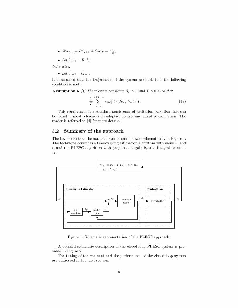
3.2 Summary of the approach

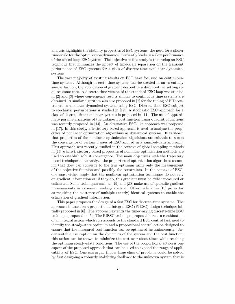
The key elements of the approach can be summarized schematically in Figure 1.The technique combines a time-varying estimation algorithm with gains K andα and the PI-ESC algorithm with proportional gain kg and integral constantτI .

Parameter Estimator

yk kek uk

pre-condition

yk

-predict output

!k

parameter update PI controller

Control Law

xk+1 = xk + f(xk) + g(xk)uk

yk = h(xk)

Figure 1: Schematic representation of the PI-ESC approach.

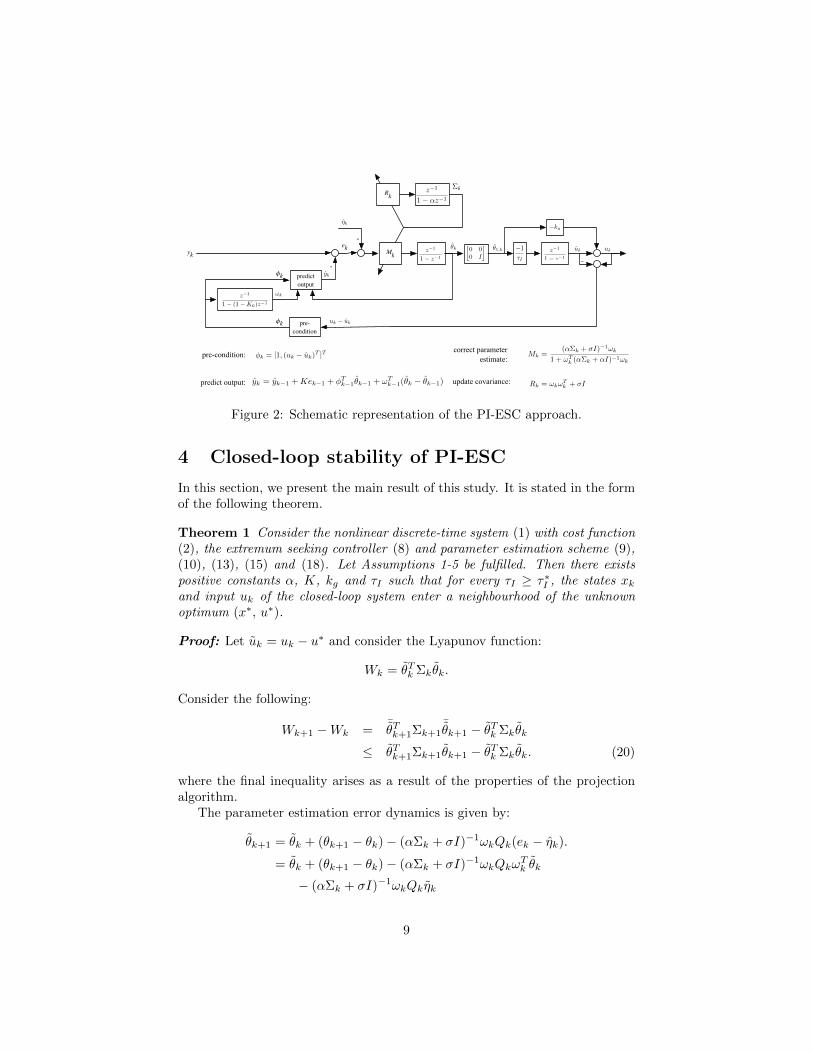
A detailed schematic description of the closed-loop PI-ESC system is pro-vided in Figure 2.

The tuning of the constant and the performance of the closed-loop systemare addressed in the next section.

8

ykk

Mkek

Rk

yk = yk1 + Kek1 + Tk1k1 + !T

k1(k k1)predict output:

correct parameterestimate:

update covariance:

uk uk1,k z1

1 z1

1

I

kg

k

-

-

uk ukpre-condition

!k

!k

yk

-predict output

z1

1 z1

pre-condition:

0 00 I

!k

z1

1 (1 Kk)z1

z1

1 ↵z1

Mk =(↵k + I)1!k

1 + !Tk (↵k + ↵I)1!k

Rk = !k!Tk + I

k = [1, (uk uk)T ]T

k

Figure 2: Schematic representation of the PI-ESC approach.

4 Closed-loop stability of PI-ESC

In this section, we present the main result of this study. It is stated in the formof the following theorem.

Theorem 1 Consider the nonlinear discrete-time system (1) with cost function(2), the extremum seeking controller (8) and parameter estimation scheme (9),(10), (13), (15) and (18). Let Assumptions 1-5 be fulfilled. Then there existspositive constants α, K, kg and τI such that for every τI ≥ τ∗I , the states xkand input uk of the closed-loop system enter a neighbourhood of the unknownoptimum (x∗, u∗).

Proof: Let uk = uk − u∗ and consider the Lyapunov function:

Wk = θTk Σkθk.

Consider the following:

Wk+1 −Wk =¯θTk+1Σk+1

¯θk+1 − θTk Σkθk

≤ θTk+1Σk+1θk+1 − θTk Σkθk. (20)

where the final inequality arises as a result of the properties of the projectionalgorithm.

The parameter estimation error dynamics is given by:

θk+1 = θk + (θk+1 − θk)− (αΣk + σI)−1ωkQk(ek − ηk).

= θk + (θk+1 − θk)− (αΣk + σI)−1ωkQkωTk θk

− (αΣk + σI)−1ωkQkηk

9

Note that by construction one can write the parameter estimation error dynam-ics as follows:

θk+1 = (θk+1 − θk) + Σ−1k+1(αΣk + σI)θk − (αΣk + σI)−1ωkQkηk

In the following, we define vk = (θk+1 − θk) − (αΣk + σI)−1ωkQkηk. Uponsubstitution of the dynamics of θk, one obtains:

θk+1 =Σ−1k+1(αΣk + σI)

[Σ−1k (αΣk−1 + σI)θk−1 + vk−1

]+ vk (21)

One obtains the following by induction:

θk+1 =

k∏

i=0

[Σ−1k−i+1(αΣk−i + σI)

]θ0 +

k∑

i=0

i∏

j=0

[Σ−1k−j+1(αΣk−j + σI)

]vk−i

where we apply the convention∏0j=0

[Σ−1k−j+1(αΣk−j + σI)

]= 1.

θk+1 =Σ−1k+1

k∏

i=1

[(αΣk−i + σI)Σ−1

k−i]

(αΣ0 + σI)θ0 +

k∑

i=0

i∏

j=0

[Σ−1k−j+1(αΣk−j + σI)

]vk−i

=Σ−1k+1

k−1∏

i=1

[(αI + σΣ−1

k−i)]

(αΣ0 + σI)θ0 +

k∑

i=0

i∏

j=0

[Σ−1k−j+1(αΣk−j + σI)

]vk−i

The matrix Σk+1 can be bounded as follows. The recursion for Σk can berewritten as:

Σk+1 = αk+1Σ0 +

k∑

i=0

αk−iωiωTi +

k∑

i=0

αk−iσI.

Then one can write:

Σk+1 ≤ αk+1Σ0 +

k∑

i=0

αk−i

T∑

j=1

ωi+jωTi+j + σI

≤ αk+1Σ0 +

k∑

i=0

αk−iT (β + σ)I ≤ αk+1Σ0 +1− αk+1

1− α T (β + σ)I

10

Similarly, one can provide a lower bound for Σk+1. Consider the quantity:

TΣk+1 = Tαk+1Σ0 + T

k∑

i=0

αk−iωiωTi + T

k∑

i=0

αk−iσI

≥ Tαk+1Σ0 +

k∑

i=T

αk−iωiωTi +

k−1∑

i=T−1

αk−iωiωTi +

. . .+

k−T∑

i=0

αk−iωiωTi + T

k∑

i=0

αk−iσI

= Tαk+1Σ0 +

k−T∑

i=0

αk−i−Tωi+TωTi+T

+

k−T∑

i=0

αk−i−T−1ωi+T−1ωTi+T−1+

. . .+

k−T∑

i=0

αk−iωiωTi + T

k∑

i=0

αk−iσI

= Tαk+1Σ0 +

k−T∑

i=0

αk−iT−1∑

j=0

α−jωi+jωTi+j + T

k∑

i=0

αk−iσI

≥ Tαk+1Σ0 +

k−T∑

i=0

αk−iT−1∑

j=0

ωi+jωTi+j + T

k∑

i=0

αk−iσI

≥ Tαk+1Σ0 +

k−N∑

i=0

αk−iTβT I + T

k∑

i=0

αk−iσI

≥ Tαk+1Σ0 +αT − αk+1

1− α TβT I + TσI

= Tαk+1Σ0 +αT (1− αk−T+1

1− α TβT + TσI

≥ Tαk+1Σ0 +αT

1− αTβT I + TσI ≥ αT

1− αTβT I + TσI.

Assuming that Σ0 = α0I, one gets the following bounds:

αT

1− αβT I + σI ≤ Σk+1 ≤ α0I +1

1− αT (β + σ)I.

or,

1− αα0(1− α) + T (β + σ)

≤ Σ−1k+1 ≤

1− αβTαT + σ(1− α)

I. (22)

11

By the dynamics of ηk, it is easy to show that:

ηk+1 =

k∑

i=1

(1−K)k−i+1η0 +

k∑

i=1

(1−K)k−iωTi (θi+1 − θi)

The term vk can be written as:

vk =(θk+1 − θk)− (αΣk + σI)−1ωkQkηk

=(θk+1 − θk)− (αΣk + σI)−1ωkQk

(k−1∑

i=1

(1−K)k−i+1η0 +

k−1∑

i=1

(1−K)k−iωTi (θi+1 − θi))

As a result, one obtains the upper bound:

‖ηk+1‖ =

k∑

i=1

(1−K)k−i+1‖η0‖

+

k∑

i=1

(1−K)k−i‖ωi‖‖(θi+1 − θi)‖

≤k∑

i=1

(1−K)k−i+1‖η0‖

+

k∑

i=1

(1−K)k−i√β‖θi+1 − θi‖

The parameter estimation error is such that:

‖θk+1‖ ≤k∏

i=0

(α‖Σ−1

k+1−i‖‖Σk−i‖+ σ‖Σ−1k+1−i‖

)‖θ0‖

+

k∑

i=1

i∏

j=0

(α‖Σ−1

k−j+1‖‖Σk−j‖+ σ‖Σ−1k−j+1‖

)‖vi‖

≤k∏

i=0

(α

((α0 + σ)(1− α) + T (β + σ)

βTαT + σ(1− α)

))‖θ0‖

+

k∑

i=1

i∏

j=0

(α

((α0 + σ)(1− α) + T (β + σ)

βTαT + σ(1− α)

))‖vi‖.

By smoothness of Ψ0,k and Ψ1,k, there exists positive constants LΨ1, LΨ1

and LΨ1such that:

‖θi+1 − θi‖ ≤ ‖Ψ0,i+1 −Ψ0,i‖+ ‖Ψ1,i+1 −Ψ1,i‖≤ LΨ1

‖xk+1 − xk‖+ LΨ2‖uk+1 − uk‖+ LΨ3

‖(uk+1 − uk+1)− (uk − uk)‖

12

∀xk ∈ D(u) and ∀u ∈ U . Upon substitution of xk+1 uk+1 and uk+1, one obtains:

‖θi+1 − θi‖ ≤ LΨ1‖f(xk) + g(xk)(−kg θ1,k + uk + dk)‖

+LΨ2

τI‖θ1,k‖+ kgLΨ3‖θk+1 − θk‖.

By smoothness of f(x) and g(x), it follows that there exists positive constantsLF and LG such that

‖f(xk)− f(π(uk))‖ ≤ LF ‖xk − π(uk)‖, ‖g(xk)− g(π(uk))‖ ≤ LG‖xk − π(uk)‖.

As a result, one obtains the following inequality:

‖θi+1 − θi‖ ≤ LΨ1LF ‖xk − π(uk)‖+ kgLΨ1

LG‖xk − π(uk)‖‖θ1,k‖+ LΨ1LG‖xk − π(uk)‖‖dk‖

+ kgLΨ1‖g(π(uk))‖‖θ1,k‖+ LΨ1

‖g(π(uk))‖‖dk‖+LΨ2

τI‖θ1,k‖+ kgLΨ3

‖θk+1 − θk‖

Using the bounds ‖dk‖ ≤ D and ‖θk‖ ≤ L1, the following inequality results:

‖θi+1 − θi‖ ≤ (LΨ1LF + kgLΨ1

LG +DLΨ1LG)‖xk − π(uk)‖

+ kgLΨ1GL1 +DLΨ1G+L1LΨ2

τI+ 2kgLΨ3L1

or, finally,

‖θi+1 − θi‖ ≤ b1(kg, D)‖xk − π(uk)‖+ b0(kg,1

τI, D).

Without loss of generality, we also assume that ‖η0‖ = 0.Let us assume that there exists a positive constant β such that:

1

T

∑

j=1

ωk+jωtk+j ≤ βI,

for all k > 0. (By definition, the boundedness of ωk is guaranteed if uk and ukare in U .).

Then one can write:

‖θk+1‖ ≤1− αβT

αk−T+1α0‖θ0‖+ Υ(T, α,K)b1(kg, D)‖xk − π(uk)‖+ Υ(T, α,K)b0(kg,1

τI, D)

= c1 + c2‖xk − π(uk)‖

where

Υ(T, α,K) =1− αk+1

βTαTα0 +

1− αk+1

βTαT (1− α)Tβ +

(1− α)(1− αk+1(1−K)k+1)

(1−K)(βTαT )2α0β

+1− αk+1(1−K)k+1

(1−K)(βTαT )2Tβ2.

13

We thus see that the parameter estimation error will tend to a neighbourhoodof the origin. The size of this neighbourhood depends primarily on the constantT associated with the persistency of excitation condition.

As above, we pose the following Lyapunov function candidate:

V = W + h+1

2uT u.

The recursion of V yields:

Vk+1 − Vk = Wk+1 −Wk + Ψ0,k + Ψ1,k(uk − uk)

+1

2uTk+1uk+1 −

1

2u>k uk.

Substitution of the ESC yields:

Vk+1 − Vk = Wk+1 −Wk + Ψ0,k − kgΨ1,kθ1,k + Ψ1,kdk

+1

2

(uk +

1

τIθ1,k

)T (uk +

1

τIθ1,k

)− 1

2u>k uk.

Replacing θ1,k = ΨT1,k − θ1,k gives:

Vk+1 − Vk =Wk+1 −Wk + Ψ0,k − k∗gΨ1,kΨT1,k − (kg − k∗g)Ψ1,kΨT

1,k

+ kgΨ1,kθ1,k + Ψ1,kdk +1

τIu>k (ΨT

1,k − θ1,k)

+1

2τ2I

(ΨT1,k − θ1,k)>(ΨT

1,k − θ1,k)

Let kg = kg − k∗g . By Assumptions 1 and 4, one obtains:

Vk+1 − Vk ≤ −αe‖x− π(uk)‖2 −(kg −

1

2τ2I

)‖Ψ1,k‖2

+

∣∣∣∣(kg −

1

τ2I

)∣∣∣∣ ‖Ψ1,k‖‖θ1,k‖+ ‖Ψ1,k‖‖dk‖

− αuτI‖uk‖2 +

LHτI‖x− π(uk)‖‖uk‖+

1

τI‖uk‖‖θ1,k‖

+1

2τ2I

‖θ1,k‖2

where LH is the Lipschitz constant associated with

‖Ψ1,k −∇h(uk)g(π(uk))‖ ≤ LH‖x− π(uk)‖.

14

Substituting for the upper bound of ‖θk‖, one obtains

Vk+1 − Vk ≤ −αe‖x− π(uk)‖2 −(kg −

1

2τ2I

)‖Ψ1,k‖2

+

∣∣∣∣(kg −

1

τ2I

)∣∣∣∣ c1‖Ψ1,k‖+D‖Ψ1,k‖

+

∣∣∣∣(kg −

1

τ2I

)∣∣∣∣ c2‖Ψ1,k‖‖x− π(uk)‖ − αuτI‖uk‖2

+c1LHτI‖x− π(uk)‖+

c2LHτI‖x− π(uk)‖2

+c1τI‖uk‖+

(LHτI

+c2τI

)‖uk‖‖x− π(uk)‖+

c21τ2I

+c22τ2I

‖x− π(uk)‖2

Rearranging and letting kg = 1τ2I

, one obtains:

Vk+1 − Vk ≤ −[‖x− π(uk)‖ ‖uk‖ ‖Ψ1,k‖

]

×

αe − c2LHτI− c22

τ2I− c2+LH

2τI0

− c2+LH2τI

αuτI

0

0 0(

12τ2I

)− k∗g

×

‖x− π(uk)‖‖uk‖‖Ψ1,k‖

+c1LHτI‖x− π(uk)‖+

c1τI‖uk‖+D‖Ψ1,k‖+

c21τ2I

It is easy to see that there exists a τ∗I such that ∀τI > τ∗I , with kg = 1τ2I

and

k∗g <1

2τ2I

, the last inequality can be written as:

Vk+1 − Vk ≤− λ1‖x− π(uk)‖2 − λ1‖uk‖2 − λ1‖Ψ1,k‖2 +c1LHτI‖x− π(uk)‖

+c1τI‖uk‖+D‖Ψ1,k‖+

c21τ2I

for a positive constant λ1 > 0 taken as the minimum eigenvalue of the matrix:

αe − c2LHτI− c22

τ2I− c2+LH

2τI0

− c2+LH2τI

αuτI

0

0 0(

12τ2I

)− k∗g

.

By Assumption 4, one can then write the following:

Vk+1 − Vk ≤ −λ1

β2(Wk + hk)− λ1‖uk‖2 − λ1‖Ψ1,k‖2 +

c1LH√β1τI

Wk +c1τI‖uk‖+D‖Ψ1,k‖+

c22τ2I

≤ −λ2Vk − λ1‖Ψ1,k‖2 + β3

√Vk +D‖Ψ1,k‖+

c22τ2I

15

where

λ2 = min

[λ1

β2, λ1

]

and

β3 = max

[c1LHτI

1√β1,√

2c1τI

].

Thus we see that the closed-loop signals ‖Ψ1,k‖, ‖uk‖ and ‖x − π(uk)‖ ofthe proposed ESC signals enter a neighbourhood of the origin whose magnitude

depends on the magnitude of ‖dk‖. This neighbourhood will be of order O(c21τ2I

)

and O(Dλ1

).

As Vk enters a neighbourhood of the origin, it follows that the closed-loopsignals enter a neighbourhood of the optimum steady-state conditions (x∗, u∗).This completes the proof.

Remark 1 The proof provides some nominal tuning guidelines for kg and τI .If one fixes τI , the analysis suggests to pick kg = 1/τ2

I . However, it is clear thatthere is much more freedom to pick kg. To demonstrate, assume that one canpick τI large enough such that:

limτI→∞

(Vk+1 − Vk) ≤−[‖x− π(uk)‖ ‖Ψ1,k‖

]×[

αe −kgc22

−kgc22 kg

] [‖x− π(uk)‖‖Ψ1,k‖

]+ (kgc1 +D)‖Ψ1,k‖

Consequently, we see that there exists a kg such that for every kg < kg theinequality can be written as:

limτI→∞

(Vk+1 − Vk) ≤− λ3‖x− π(uk)‖ − λ3‖Ψ1,k‖2

+ (kgc1 +D)‖Ψ1,k‖

The closed-loop signals will asymptotically enter a neighbourhood of the origingiven by:

Ωkg =

x ∈ D(u) u ∈ U

∣∣∣∣ ‖Ψ1,k‖ ≤(kgc1 +D)

λ3

Thus, one can establish a maximum gain kg that retains closed-loop stabilityin the absence of integral action. Moreover, closed-loop stability can also beachieved even if the nonlinear system is only Lyapunov stable (αe = 0) for a fixeduk. This is a clear advantage of the proposed ESC over classical perturbationbased discrete-time ESC techniques that require local asymptotic stability of thenonlinear system. The problem of feedback stabilization of nonlinear discrete-time systems using ESC will be considered in future work.

16

5 Simulation

In this section, we consider the application of the PIESC approach to nonlineardiscrete-time control systems. The performance of the proposed approach iscompared to the standard perturbation based ESC algorithm proposed in [7].This algorithm is given by:

ξk+1 = −h`ξk + yk

uk+1 = uk − γα cos(ωk)(yk − (1 + h`)ξk+1)

uk = uk + α cos(ω(k + 1)).

5.1 Example 1

We first consider the application of the PI-ESC approach to the following non-linear discrete-time system:

xk+1 =0.99xk + (uk − 0.1)(1 +1

2sin(xk))

yk =1 + 0.2(xk − 1)2

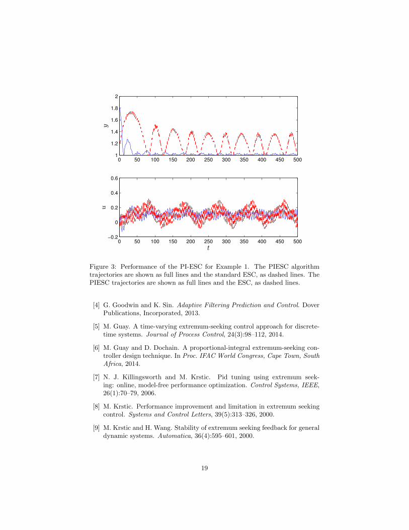
We first note that the nonlinear system has a pole very close to the unit circle.The optimum occurs at x∗ = 1, u∗ = 0.1069. The PIESC is used with again of kg = 10 and integral time constant τI = 100. The dither signal isdk = 0.05 sin(k). The estimation gates are set to K = 0.001, α = 0.001 andσ = 0.001. The simulation results are shown in Figure 3. The figure shows thecost function, yk, the input, uk, and the integration variable uk. The PIESCvery effectively converges to the optimum equilibrium conditions. The tuningparameters for the perturbation ESC are h` = 0.1, γ = 3/α, α = 0.1, ω = 2.The corresponding ESC performance is shown as the dashed line in Figure 3.As expected, the proposed PIESC provides a drastically faster convergence tothe optimum conditions. Furthermore, the impact of the slow nearly unstabledynamics are compensated by the presence of the proportional action.

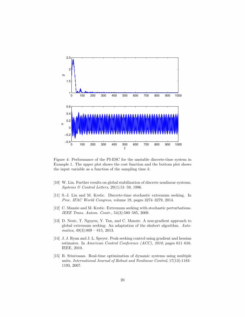
Next, we consider the following unstable nonlinear system:

xk+1 =1.01xk + (uk − 0.1)(1 +1

2sin(xk))

yk =1 + 0.2(xk − 1)2

The optimum occurs at x∗ = 1, u∗ = 0.09457. The PIESC is used with again of kg = 0.2 and integral time constant τI = 1000. The dither signal isdk = 0.5 sin(15k). The estimation gains are set to K = 0.001, α = 0.001and σ = 0.001. Figure 4 shows the simulation results. The PIESC simulta-neously stabilizes the nonlinear system and identifies the optimum equilibriumconditions. The standard perturbation based ESC technique cannot successfullyoptimize this system.

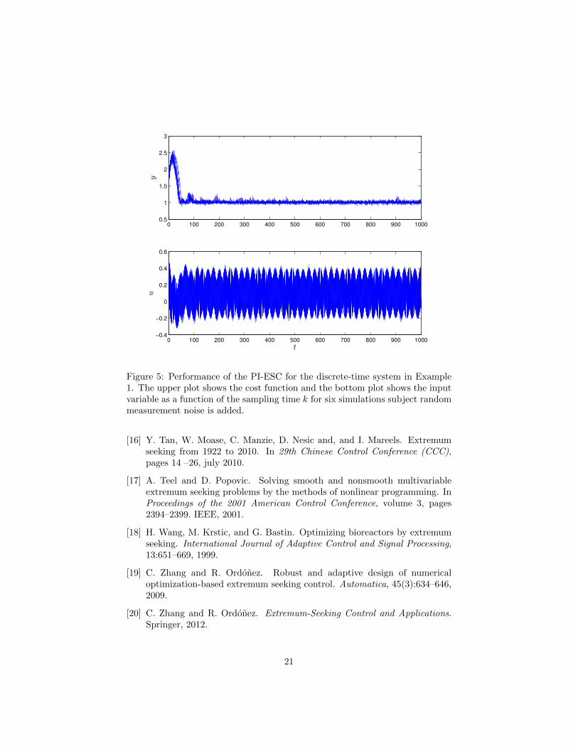
To verify the robustness of the proposed approach, random zero mean mea-surement noise is added to the cost measurement. The noise measurement is

17

given by:yk = 1 + 0.2(xk − 1)2 + 0.03νk

where νk is a zero mean, unit variance Gaussian random variable. The resultsare shown in Figure 5. Six simulations are performed. All simulation show goodtransient performance to the unknown optimum.

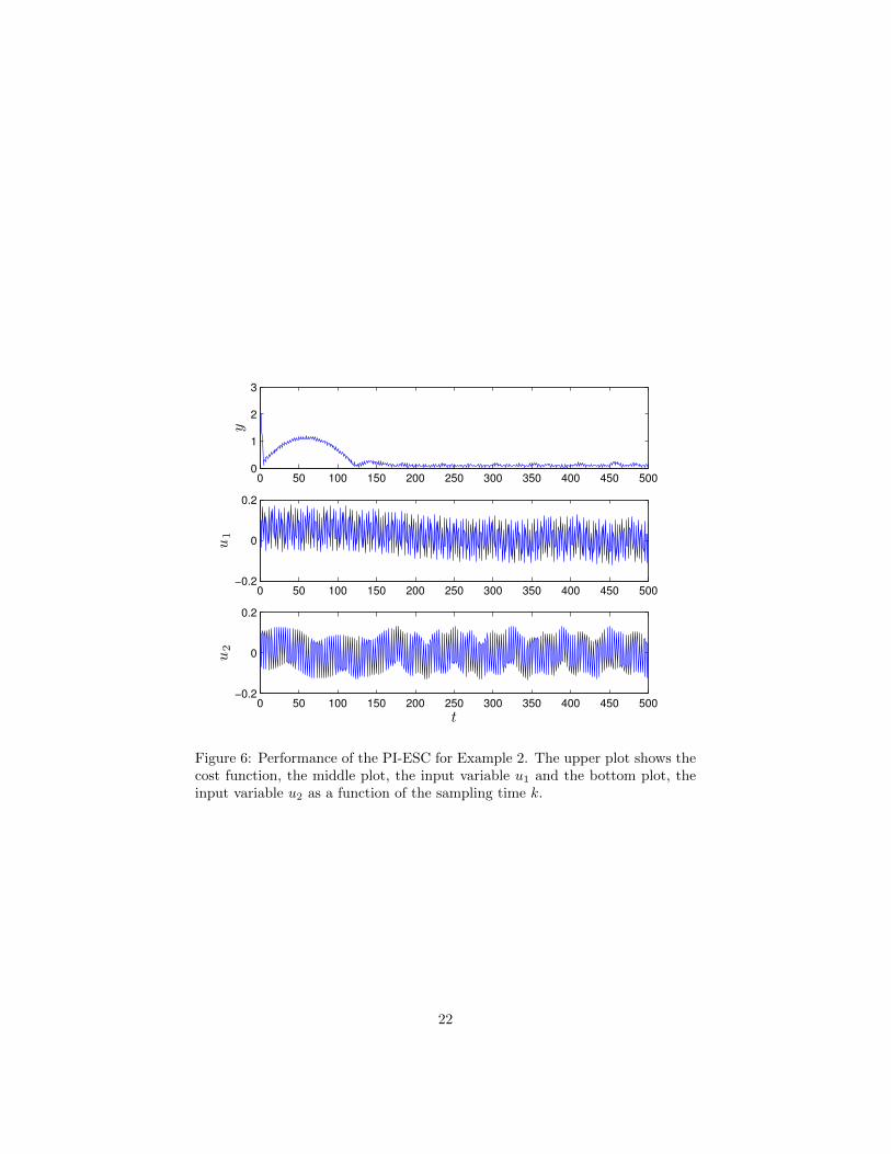
5.2 Example 2

The task is to stabilize the nonlinear discrete-time control system studied in [10]given by:

x1,k+1 = x23,k + u1,k

x2,k+1 = x2,k + u2,k

x3,k+1 = 2x3,k(u1,k + x1,kx2,ku2,k)

with cost function yk = 12 (x2

1,k + x22,k + x2

3,k).

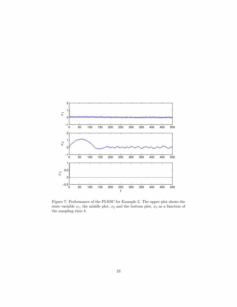
The optimum occurs at x∗ = [0, 0, 0]T , u∗ = [0, 0]T . The PIESC is usedwith a gain of kg = 0.5 and integral time constant τI = 50. The dither signalis dk = [0.2 sin(450k), 0.2 sin(400k)]T . The estimation gates are set to K =0.001, α = 0.01 and σ = 0.01. Figure 6 shows the output function along withthe two inputs. The corresponding state trajectories are shown in Figure 7.The PIESC simultaneously stabilizes the nonlinear system and identifies theoptimum equilibrium conditions.

6 Conclusion

This paper proposes a proportional-integral extremum-seeking control techniquefor a class of discrete-time nonlinear dynamical systems with unknown dynam-ics. The main contribution of this technique is the minimization of the impactof time-scale separation on the transient performance of the extremum-seekingcontrol system in discrete-time.

References

[1] K. Ariyur and M. Krstic. Analysis and design of multivariable extremumseeking. In Proceedings of the American Control Conference, pages 2903–2908, Anchorage, 2002.

[2] K. B. Ariyur and M. Krstic. Real-time optimization by extremum-seekingcontrol. Wiley-Interscience, 2003.

[3] J.-Y. Choi, M. Krstic, K. Ariyur, and J. Lee. Extremum seeking control fordiscrete-time systems. IEEE Trans. Autom. Contr., 47(2):318–323, 2002.

18

0 50 100 150 200 250 300 350 400 450 5001

1.2

1.4

1.6

1.8

2

y

0 50 100 150 200 250 300 350 400 450 500−0.2

0

0.2

0.4

0.6

u

t

Figure 3: Performance of the PI-ESC for Example 1. The PIESC algorithmtrajectories are shown as full lines and the standard ESC, as dashed lines. ThePIESC trajectories are shown as full lines and the ESC, as dashed lines.

[4] G. Goodwin and K. Sin. Adaptive Filtering Prediction and Control. DoverPublications, Incorporated, 2013.

[5] M. Guay. A time-varying extremum-seeking control approach for discrete-time systems. Journal of Process Control, 24(3):98–112, 2014.

[6] M. Guay and D. Dochain. A proportional-integral extremum-seeking con-troller design technique. In Proc. IFAC World Congress, Cape Town, SouthAfrica, 2014.

[7] N. J. Killingsworth and M. Krstic. Pid tuning using extremum seek-ing: online, model-free performance optimization. Control Systems, IEEE,26(1):70–79, 2006.

[8] M. Krstic. Performance improvement and limitation in extremum seekingcontrol. Systems and Control Letters, 39(5):313–326, 2000.

[9] M. Krstic and H. Wang. Stability of extremum seeking feedback for generaldynamic systems. Automatica, 36(4):595–601, 2000.

19

0 100 200 300 400 500 600 700 800 900 10001

1.5

2

2.5

y

0 100 200 300 400 500 600 700 800 900 1000−0.4

−0.2

0

0.2

0.4

0.6

u

t

Figure 4: Performance of the PI-ESC for the unstable discrete-time system inExample 1. The upper plot shows the cost function and the bottom plot showsthe input variable as a function of the sampling time k.

[10] W. Lin. Further results on global stabilization of discrete nonlinear systems.Systems & Control Letters, 29(1):51–59, 1996.

[11] S.-J. Liu and M. Krstic. Discrete-time stochastic extremum seeking. InProc. IFAC World Congress, volume 19, pages 3274–3279, 2014.

[12] C. Manzie and M. Krstic. Extremum seeking with stochastic perturbations.IEEE Trans. Autom. Contr., 54(3):580–585, 2009.

[13] D. Nesic, T. Nguyen, Y. Tan, and C. Manzie. A non-gradient approach toglobal extremum seeking: An adaptation of the shubert algorithm. Auto-matica, 49(3):809 – 815, 2013.

[14] J. J. Ryan and J. L. Speyer. Peak-seeking control using gradient and hessianestimates. In American Control Conference (ACC), 2010, pages 611–616.IEEE, 2010.

[15] B. Srinivasan. Real-time optimization of dynamic systems using multipleunits. International Journal of Robust and Nonlinear Control, 17(13):1183–1193, 2007.

20

0 100 200 300 400 500 600 700 800 900 10000.5

1

1.5

2

2.5

3

y

0 100 200 300 400 500 600 700 800 900 1000−0.4

−0.2

0

0.2

0.4

0.6

u

t

Figure 5: Performance of the PI-ESC for the discrete-time system in Example1. The upper plot shows the cost function and the bottom plot shows the inputvariable as a function of the sampling time k for six simulations subject randommeasurement noise is added.

[16] Y. Tan, W. Moase, C. Manzie, D. Nesic and, and I. Mareels. Extremumseeking from 1922 to 2010. In 29th Chinese Control Conference (CCC),pages 14 –26, july 2010.

[17] A. Teel and D. Popovic. Solving smooth and nonsmooth multivariableextremum seeking problems by the methods of nonlinear programming. InProceedings of the 2001 American Control Conference, volume 3, pages2394–2399. IEEE, 2001.

[18] H. Wang, M. Krstic, and G. Bastin. Optimizing bioreactors by extremumseeking. International Journal of Adaptive Control and Signal Processing,13:651–669, 1999.

[19] C. Zhang and R. Ordonez. Robust and adaptive design of numericaloptimization-based extremum seeking control. Automatica, 45(3):634–646,2009.

[20] C. Zhang and R. Ordonez. Extremum-Seeking Control and Applications.Springer, 2012.

21

0 50 100 150 200 250 300 350 400 450 5000

1

2

3

y

0 50 100 150 200 250 300 350 400 450 500−0.2

0

0.2

u1

0 50 100 150 200 250 300 350 400 450 500−0.2

0

0.2

u2

t

Figure 6: Performance of the PI-ESC for Example 2. The upper plot shows thecost function, the middle plot, the input variable u1 and the bottom plot, theinput variable u2 as a function of the sampling time k.

22

0 50 100 150 200 250 300 350 400 450 500−1

0

1

2

x1

0 50 100 150 200 250 300 350 400 450 500−1

0

1

2

x2

0 50 100 150 200 250 300 350 400 450 500−0.5

0

0.5

1

x3

t

Figure 7: Performance of the PI-ESC for Example 2. The upper plot shows thestate variable x1, the middle plot, x2 and the bottom plot, x3 as a function ofthe sampling time k.

23