MAXIMUM POWER POINT TRACKING FOR PHOTOVOLTAIC OPTIMIZATION

USING RIPPLE-BASED EXTREMUM SEEKING CONTROL

Steven L. Brunton1, Clarence W. Rowley1, Sanjeev R. Kulkarni1, and Charles Clarkson2

1Princeton University, Princeton, NJ 08544

2ITT Space Systems Division, Rochester, NY 14606

December 14, 2009

Corresponding Author: Steven Brunton

e-Mail: sbrunton@Princeton.Edu

Phone: (609)-921-6415

Fax: (609)-258-6109

Address: Steven Brunton

MAE Department

D-wing, Engineering Quadrangle

Princeton University

Princeton, NJ 08544

Parts of this work were presented at the 34th IEEE Photovoltaic Specialists Conference in Philadelphia on June 7-12, 2009.

Keywords: Maximum power point tracking, extremum seeking, rapidly varying irradiance, inverter ripple, photovoltaic power

generation

Abstract

This work develops a maximum power point tracking (MPPT) algorithm that optimizes solar array perfor-

mance and is robust to rapidly varying irradiance conditions. In particular, a novel extremum seeking (ES)

controller which utilizes the natural inverter ripple is designed and tested on a simulated solar array with a

grid-tied inverter. The new algorithm is benchmarked against the perturb and observe (PO) method using

high-variance irradiance data gathered on a rooftop array experiment in Princeton, NJ. The extremum seeking

controller achieves efficiencies exceeding 99% with transient rise-time to the MPP of less than .1 seconds.

It is shown that voltage-control is more stable than current-control and allows for accurate tracking of faster

irradiance transients. The limitations of current-control are demonstrated on an example. Finally, the effect of

capacitor size on the performance of ripple-based extremum seeking control is investigated.

1

1 INTRODUCTION

Recently, there has been significant environmental and political motivation to shift domestic power generation to renew-

able sources such as wind and solar. Solar power is at the forefront of clean, renewable energy, and it is gaining momentum

due to advances in solar panel manufacturing and efficiency as well as increasingly volatile fuel costs. Solar power is an

attractive option because of the large amount of power available in incident sunlight, particularly in large industrial parks

and residential suburbs. However, photovoltaic (PV) solar cells, the most readily available solar technology, operate best

on bright days with little or no obstruction to incident sunlight. Frequent overcast days and partial obstructions such as tree

limbs or neighboring buildings limit the efficiency and reliability of solar power throughout much of the United States [18].

This work is motivated by the need to optimize solar array performance for rapidly varying environmental conditions, such

as those characteristic of New Jersey’s climate.

Because of the photovoltaic nature of solar panels, the current-voltage, or I-V , curves depend nonlinearly on tempera-

ture and irradiance levels [10, 21]. Therefore, the operating current and voltage which maximize power output will change

with environmental conditions, as in Fig. 2. In order to maintain efficient operation despite environmental variations, one

approach is to use a maximum power point tracking (MPPT) algorithm to dynamically tune either control current or voltage

to the maximum power operating point.

Typically MPPT algorithms are implemented on a solar array using a switching power converter. For example, with a

grid-tied inverter, the solar array charges a capacitor, and then current is switched out of the capacitor at a varying duty

cycle in order to reconstruct a sinusoidal current which injects power into the grid. A number of solar power converter

architectures are discussed in the literature [1, 2, 15, 17, 20]. In the majority of power converters, the internal switching

mechanism imposes a voltage and current ripple which is felt by the PV array. Minimizing the magnitude of this ripple has

been a major concern, and is achieved by careful (and expensive) choice of the capacitor and inductor.

There are a number of maximum power point tracking algorithms for changing environmental conditions [9, 6]. Control

algorithms which do not assume a particular model and are robust to uncertain system parameters are ideal for a number

of reasons, including less frequent maintenance and fine tuning. Robust, model independent algorithms are applicable to a

wide range of panel and inverter technologies. A number of “black box” MPPT algorithms, such as perturb and observe [9]

and incremental conductance [10] have been explored in the literature [6].

Perturb and observe (PO) is a workhorse MPPT algorithm because of its balance between performance and simplicity.

In its simplest form, the perturb and observe algorithm tracks the MPP by perturbing the control input in a given direction

and observing if the output power goes up or down; if the power increases, the perturbation direction is unchanged, and if

the power decreases, the direction is reversed. Because the standard perturb and observe method uses a fixed perturbation

size, it suffers from a performance tradeoff between transient rise-time and steady-state performance. PO has also been

shown to track in the wrong direction given rapidly varying irradiance [6]. Modified versions of PO have been proposed,

2

for example by using an adaptive step which is related to ∆P/∆u (where P is power and u is either perturbed voltage or

current) [8] or by including rudimentary model assumptions [7].

A promising new MPPT algorithm is the method of extremum seeking (ES) control, which may be closely related to the

ripple correlation control (RCC) and PO methods. The extremum seeking method of Krstic [11] offers fast convergence

and good steady state performance with guaranteed stability for a range of parameters. [12] and [3] implement extremum

seeking control by injecting an external perturbation signal. Ripple correlation control (RCC) utilizes the natural inverter

ripple and corrects the duty cycle of the switching converter in order to set P I = 0, which is a condition for the MPP. The

duty cycle is updated using either a discrete comparison, as in perturb and observe [13, 14, 19], or using the product of the

high-pass filtered power and control variable, as in extremum seeking control [16, 5].

The approach here is to develop an extremum seeking controller that utilizes the natural 120Hz inverter ripple to track the

MPP in rapidly varying irradiance conditions. In particular, the extremum seeking controller is compared against a well-tuned

PO algorithm on high-variance irradiance data measured for use on a solar array on the roof of Princeton’s engineering quad.

This work also compares the use of voltage and current as control variables and demonstrates limitations of current-control

for gradient-climb methods. Finally, the effect of capacitor size on extremum seeking control is investigated.

2 PV ARRAY INVERTER MODEL

In order to simulate a comparison of various MPPT algorithms, it is necessary to model the array-inverter dynamics.

Figure 1 is a schematic of the array-inverter system. The block labelled PV Array encapsulates all of the dynamics associ-

ated with the solar array, including the functional dependence of the I-V curves with irradiance G and temperature T . The

switching dynamics of the inverter are encapsulated in the block labelled u, and are discussed below. L and C represent

the inductor and capacitor, respectively.

PV

Arrayu C

L

I

V

Figure 1: Schematic of PV array and inverter with LC dynamics. The inverter control variable u is either currentor voltage and is controlled by the inverter’s switching logic.

3

2.1 PV Array Model

The array I-V curve may be written I = I(V,G, T ) and is modeled by the lighted-diode equations [10, 21]:

I = IL − IOS»exp

q

AkBT(V + IR)− 1

–(1)

IOS = IOR

„T

TR

«exp

„qEGAkB

„1

TR− 1

R

««(2)

IL =G

1000(ISC +KT,I(T − TR)) (3)

where I and V are the same as in Figure 1, IL is the light generated current, IOS is the cell reverse saturation current, and T

is temperature. Because temperature variations are typically much more gradual than irradiance changes, we assume that

temperature is constant, Tconst = 300K, for the remainder of the analysis. Thus the functional dependence on T is dropped.

V = V (I,G) , V (I,G, Tconst) (4)

I = I(V,G) , I(V,G, Tconst) (5)

are equivalent representations of the I-V curves for a constant temperature Tconst and changing irradiance G.

Values and definitions of other terms in the equations are as follows: TR = 298 (reference temperature), IOR = 2.25e−6

(reverse saturation current at T = TR), ISC = 3.2 (short-circuit current), EG = 1.8e−19 (Silicon band gap), A = 1.6 (ideality

factor), kB = 1.38e − 23 (Boltzmann’s constant), q = 1.6e − 19 (electronic charge), R = .01 (resistance), and KT,I = .8

(short-circuit current temperature coefficient). Finally, the model array consists of 3 parallel strings, each with 7 panels

connected in series. Each panel produces approximately 220W at full irradiance, G = 1000 W/m2.

Figure 2 shows the I-V , P -V and P -I curves for varying irradiance G using the above equations and parameters.

The P -V characteristic curves are more symmetrical about the maximum power input than the P -I curves. Moreover, the

maximum power point occurs at a smaller normalized voltage input, giving voltage-control larger failure margins.

2.2 Inverter Model

Applying Kirchoff’s law to the circuit in Figure 1 yields the following relationships:

I = u+ IC (6)

VC = −V − VL (7)

where the inverter control variable u is either current, uI , or voltage, uV .

4

0 50 100 150 200 250 300 350 4000

5

10

15

Voltage (V)

Cur

rent

(I)

I−V Curves for Varying Irradiance G

0 0.2 0.4 0.6 0.8 10

1000

2000

3000

4000

5000

Normalized Input (V or I)

Pow

er (

P)

P−V and P−I Curves for Varying Irradiance G

P−V curveP−I curve

Figure 2: (left) I-V curves at several irradiance levels from G = 50 W/m2 to G = 1000 W/m2 (spaced 50 W/m2

apart). (right) P -V (black) and P -I (gray) curves at several irradiance levels, plotted with respect to an inputvariable which is normalized by its maximum allowable value. The maximum power point is labeled on eachplot as either a black circle or gray diamond.

If the inverter control variable is current, uI , the array I-V curve has the form V = V (I,G) and equation (7) becomes:

VC = −V (I,G)− LdIdt

(8)

=⇒ −dVCdt

=d

dtV (I,G) + L

d2I

dt2(9)

=∂V (I,G)

∂I

dI

dt+∂V (V,G)

∂G

dG

dt+ L

d2I

dt2(10)

Equation (6) and the capacitor equation yield:

dVCdt

=ICC

=⇒ dVCdt

= − 1

C(uI − I) (11)

Combining equations (10) & (11) yields the system dynamics in terms of inverter control current uI and array current I:

LCd2I

dt2+ C

∂V

∂I

dI

dt+ I = uI − C

∂V

∂G

dG

dt(12)

The dynamical system given by equation (12) represents a forced oscillator with nonlinear damping. The forcing

corresponds to the inverter control current uI as well as the change in I-V curve due to irradiance change, given by

−C(∂V/∂G)(dG/dt).

To flow 60Hz AC power into the grid at a given current uI , the inverter switches DC current out of a large capacitor. This

5

requires the following inverter control current with a large 120Hz oscillation:

uI = uI (1 + sin(120× 2πt)) (13)

In practice, the LC circuit acts as a low pass filter between the control current uI , and the array current I, so that I

experiences a 120Hz ripple at approximately 3% magnitude:

I ≈ uI (1 + .03 sin(120× 2πt+ ϕ)) (14)

There is also a high frequency ripple at 20kHz due to the inverter sampling time; however, this has a negligible effect

and is not modeled. For more information on DC-AC power inverters, see Bose [2].

Similarly, if the inverter control variable is voltage, uV , the array I-V curve has the form I = I(V,G), which yields the

following voltage-control dynamics

L∂I

∂VV + V = −uV − L

∂I

∂GG (15)

Notice that the system type and order of the current-control dynamics (12) and voltage-control dynamics (15) are differ-

ent. This difference is due to the fact that the control voltage is instantaneously reflected in the capacitor voltage.

3 MAXIMUM POWER POINT TRACKING

In the maximum power point tracking (MPPT) algorithms implemented below, it is assumed that there are current and

voltage measurements which may be multiplied to obtain a power measurement. The control variable is either current or

voltage, which are determined by the MPPT algorithm and commanded by the inverter. The algorithms do not require any

additional sensors or models to track the MPPT despite exogenous disturbances due to changing irradiance, G(t).

Although there are a number of MPPT algorithms that have been developed over the past two decades, this analysis

compares a new method, ripple-based extremum seeking (ES) control, with the standard method, perturb and observe

(PO). Additionally, an interesting relationship between the existing ripple correlation control (RCC) method and extremum

seeking control is demonstrated.

The efficiency of each method is given by the formula

ηMPPT =

R t0Pactual(τ)dτR t

0Pmax(τ)dτ

(16)

and the transient rise-time, τrise, is the time it takes the algorithm to reach 90% of the instantaneous maximum power point.

6

3.1 Perturb and Observe

The most prevalent MPPT algorithm is perturb and observe (PO). PO repeatedly perturbs the input by a fixed amount

in a given direction, and the direction is changed only if a drop in power is detected. Although this algorithm benefits from

simplicity, it lacks the speed and adaptability necessary for tracking fast transients in irradiance.

A simple variant of the PO method uses an average power for the comparison step that has been averaged over a

number of inverter switching cycles. The effect of this averaged power comparison is a decrease in noise, and also that the

perturbation magnitude no longer must exceed that of the natural ripple. This is the version of PO used in this comparison.

Finally, it is possible to construct a PO algorithm with an adaptive step

∆uk+1 = ∆uk +∆Pk∆uk

(17)

This overcomes the tradeoff between transient rise and steady-state tracking efficiency. However, there are no guaranteed

stability conditions for this algorithm, and it is not implemented in this study.

3.2 Extremum Seeking Control

A robust new maximum power point tracking algorithm is based on the extremum seeking (ES) control method. A

schematic of the algorithm is shown in Figure 3. This controller converges at a rate which is proportional to the slope of

the power curve, either P -I or P -V , and has guaranteed stability over a range of system parameters [11, 4]. The algorithm

works by adding a perturbation signal α sinωt to the “best guess” for the input u which maximizes the quantity of interest,

namely the array output power. The perturbation passes through the system and produces a perturbation in the power.

Multiplying the high-pass filtered control variable (I or V ) and high-pass filtered power results in a demodulated signal ξ

which is positive to the left of the MPP and negative to the right of the MPP. Integrating this signal and adding it to the best

guess u causes the control variable u to adaptively track the MPP. A simple averaging analysis, which assumes constant

environmental conditions, shows that the demodulated signal ξ is proportional to the slope of the power curve:

ξavg =ω

2π

Z 2π/ω

0

uhp · Php dτ (18)

≈ ∂P

∂u(u, G) · α2 sin2 ωt. (19)

In practice, rather than injecting a sinusoidal control perturbation α sinωt, as in the standard extremum seeking algo-

rithm, it is convenient to utilize the inverter ripple for the perturbation. Using the control signal in equation (13), the array

current and power will have a small ripple, as in equation (14). Therefore, the high-pass filtered array current and power are

multiplied, yielding the demodulated signal, ξ, similar to Figure 3. A schematic of the new ripple-based extremum seeking

7

Solar Array &Inverter Hardware

ss+!h

"s !+

current power

high-pass lter

integrator

!"

# sin $t

u

Figure 3: Extremum seeking algorithm.

algorithm is shown in Figure 4.

Solar Array &

Inverter Hardware

ss+ωh

γs

command

current array power

integrator

ξu

array current

ss+ωh

high-pass

filters××

1 + sin ωt

Ihp

Php

Figure 4: Extremum seeking algorithm utilizing natural inverter ripple.

3.3 Ripple Correlation Control

Ripple correlation control (RCC) utilizes the natural inverter ripple to either perform perturb and observe [13, 14, 19] or

extremum seeking control [16, 5]. RCC corrects the duty cycle of the switching converter according to the integral:

d(t) = k

ZdP

dt· dIdtdt ≈ k

ZPhp · Ihpdt (20)

where Php and Ihp are first-order high-pass filtered quantities that approximate the derivatives in Eq. (20). Using this varying

duty cycle, RCC tracks the maximum power point by tracking the equivalent condition P I = 0. In practice, this imple-

mentation of RCC is similar to the ES algorithm with first order high-pass filters. However, RCC lacks the mathematical

foundation and careful stability analysis that makes extremum seeking attractive for robust design. RCC is limited to first

order high-pass filters, which approximate the derivative at low frequencies, whereas ES also works with higher order filters.

8

4 SIMULATED MPPT COMPARISON

This section summarizes the results of a simulated maximum power point tracking (MPPT) comparison between the

extremum seeking (ES) and perturb and observe (PO) algorithms. The algorithms are tested on rapidly varying irradiance

data from measurements on an partially cloudy day. Temperature is assumed constant throughout the simulations because

variations in temperature are more gradual than in irradiance. This simplifies the dynamic models (12) and (15). Two sets

of algorithm comparisons are simulated, depending on whether voltage or current is controlled by the inverter.

Using the irradiance measurements as an input to the model, both the extremum seeking (ES) and perturb and observe

(PO) algorithms are tested. The extremum seeking model is shown in Figure 4.

4.1 Irradiance Data

Figure 5 shows irradiance data for two consecutive days in June, 2007. The data was measured on a rooftop of the

Engineering Quadrangle at Princeton University. Irradiance is more erratic on the second day because of rapidly moving,

scattered cloud cover. The bottom of Fig. 5 provides a detailed view of the irradiance data over a 25 minute window between

12:34-12:59AM on June 20th, 2007 (day 2). This time range is chosen because it includes rapid irradiance changes, and

because a short 25 minute window makes it possible to see the controller response to individual irradiance changes.

The noisy irradiance measurements are low-pass filtered so that the data is averaged over about 10 seconds. Because

the irradiance sensors are located at points along the array, the measured irradiance responds more quickly to disturbances

than the array. Determining the actual time scales on which irradiance changes effect a solar array will depend on the size

and orientation of the array, and should be investigated further. Both unfiltered and low-pass filtered irradiance sets are used

in the simulations below.

9

! "!! #!!! #"!!

$!!

%!!

#!!!

#&!!

'()*+,-./

0..12(134*+,56)

&/

+

+

738(9:*.*2

9;<!=1>>

" #! #" &!!

&!!

?!!

$!!

%!!

#!!!

#&!!

#?!!

'()*+,>/

0..12(134*+,56)

&/

+

+

21@+#

21@+&

Figure 5: (top) Irradiance data for two days in June in Princeton, NJ. (bottom) Irradiance data spanning 25minutes from 12:34-12:59AM on June 20th, 2007. Signal is low-pass filtered (black), so that noisy measurements(gray) are averaged over about 10 seconds.

4.2 Voltage-Control

Figure 6 shows the results from a MPPT comparison where the inverter control variable is voltage. The array power,

current and voltage are plotted in time for the ES (black) and PO (light gray) algorithms as well as the true maximum power

(dark gray). Both PO and ES command a control voltage which oscillates closely around the true maximum power voltage,

as seen in the bottom plot. The extremum seeking method accurately tracks the maximum power point and rises to the MPP

orders of magnitude more rapidly than perturb and observe.

In the voltage-control simulation, each algorithm tracks the MPPT of the unfiltered irradiance measurements. The unfil-

tered irradiance data varies more rapidly than the filtered data, and therefore the MPPT is more difficult to track. However,

voltage-control results in almost perfect MPPT with both ES and PO achieving efficiencies around 99%. ES has efficiency

ηES = .9968 and rises to the MPP in .1s, and PO has efficiency ηPO = .9939 and rises to the MPP in 6s. The inverter

hardware uses a 2000µF capacitor and 1µH inductor. The PO step size is ∆V = 5V with 1kHz sampling. Finally, ES utilizes

the natural inverter ripple, which has magnitude 3%.

10

0 500 1000 15002000

3000

4000

5000

6000

Time (s)

Pow

er (

W)

MPPESPO

0 500 1000 15005

10

15

Time (s)

Cur

rent

(I)

0 500 1000 1500

300

350

400

Time (s)

Vol

tage

(V

)

Figure 6: Comparison of voltage-controlled extremum seeking (ES, black) and perturb and observe (PO, lightgray) controllers on 25 minutes of unfiltered irradiance data from 12:34-12:59PM. (top) Both controllers accu-rately track the MPP (dark gray) which is varying with irradiance. Plots of commanded array current (middle)and array voltage (bottom) as a function of time show the large variation in maximum power current (MPI) withirradiance, and the relative stability of the maximum power voltage (MPV).

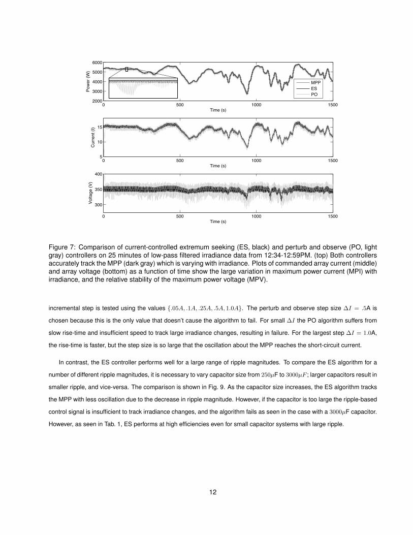
4.3 Current-Control

Figure 7 shows the results from a MPPT comparison where the inverter control variable is current. The array power,

current and voltage are plotted in time for the ES (black) and PO (light gray) algorithms as well as the true maximum power

(dark gray). The extremum seeking method commands a control current which oscillates closely around the true maximum

power current, as seen in the middle plot.

In the current-control simulation, each algorithm tracks the MPPT of the low-pass filtered irradiance data. The current-

control dynamics are not easily controllable and fail for the rapid irradiance changes found in the unfiltered data. However,

on the low-pass filtered data, current-control with PO and ES admits almost perfect MPPT. ES has efficiency ηES = .9963

with rise-time of .02s, and PO has efficiency .9898 with rise-time of 6.9 seconds. The step size for PO is ∆I = .5A.

Although both ES and PO track the maximum power point with high efficiency, ES is a more robust algorithm. This is

seen in Fig. 8, where a number of PO algorithms are compared on an array-inverter system with a 2000µF capacitor. The

11

0 500 1000 15002000

3000

4000

5000

6000

Time (s)

Power (W

)

MPP

ES

PO

0 500 1000 15005

10

15

Time (s)

Current (I)

0 500 1000 1500

300

350

400

Time (s)

Voltage (V)

Figure 7: Comparison of current-controlled extremum seeking (ES, black) and perturb and observe (PO, lightgray) controllers on 25 minutes of low-pass filtered irradiance data from 12:34-12:59PM. (top) Both controllersaccurately track the MPP (dark gray) which is varying with irradiance. Plots of commanded array current (middle)and array voltage (bottom) as a function of time show the large variation in maximum power current (MPI) withirradiance, and the relative stability of the maximum power voltage (MPV).

incremental step is tested using the values {.05A, .1A, .25A, .5A, 1.0A}. The perturb and observe step size ∆I = .5A is

chosen because this is the only value that doesn’t cause the algorithm to fail. For small ∆I the PO algorithm suffers from

slow rise-time and insufficient speed to track large irradiance changes, resulting in failure. For the largest step ∆I = 1.0A,

the rise-time is faster, but the step size is so large that the oscillation about the MPP reaches the short-circuit current.

In contrast, the ES controller performs well for a large range of ripple magnitudes. To compare the ES algorithm for a

number of different ripple magnitudes, it is necessary to vary capacitor size from 250µF to 3000µF ; larger capacitors result in

smaller ripple, and vice-versa. The comparison is shown in Fig. 9. As the capacitor size increases, the ES algorithm tracks

the MPP with less oscillation due to the decrease in ripple magnitude. However, if the capacitor is too large the ripple-based

control signal is insufficient to track irradiance changes, and the algorithm fails as seen in the case with a 3000µF capacitor.

However, as seen in Tab. 1, ES performs at high efficiencies even for small capacitor systems with large ripple.

12

0 500 1000 15000

1000

2000

3000

4000

5000

6000

Time (s)

Pow

er (

W)

MPPPO ∆I = 1.0PO ∆I = .50PO ∆I = .25PO ∆I = .10PO ∆I = .05

0 500 1000 15000

5

10

15

20

Time (s)

Cur

rent

(A

)

Figure 8: Comparison of perturb and observe (PO) controllers, using current-control, with varying perturbationstep size ∆I. As the perturbation size increases, the PO algorithm has faster rise-time, but larger oscillationsabout the maximum power point. The only PO algorithm which is able to track every irradiance change hasperturbation ∆I = .5A, resulting in high efficiency ηPO = .9898.

13

0 500 1000 15000

1000

2000

3000

4000

5000

6000

Time (s)

Pow

er (

W)

MPPCap = 500µFCap = 1000µFCap = 2000µFCap = 3000µF

0 500 1000 15000

5

10

15

20

Time (s)

Cur

rent

(A

)

Figure 9: Comparison of extremum seeking (ES) controllers, using current-control, on inverters with varyingcapacitor sizes. As capacitor size increases the ES algorithm tracks the MPP with less oscillation, due to thedecreased ripple magnitude. However, if the capacitor is too large the ripple-based control signal is insufficientto track rapid irradiance changes, and the algorithm fails, as seen when the capacitor is 3000µF. There is not anappreciable drop in performance between a 1000µF and 2000µF capacitor.

Capacitor Size (µF) 250 500 1000 2000 3000ES Efficiency (%) 90.71 96.79 98.99 99.63 N/A

Table 1: Extremum Seeking efficiency for varying inverter capacitor sizes.

14

4.4 Limitations of Current-Control

As irradiance decreases rapidly, the I-V curve shrinks and the maximum power voltage (MPV) and current (MPI) de-

crease. If the MPPT algorithm does not track fast enough, the control current or voltage will “fall off” the I-V curve. Figure 10

shows irradiance plotted against the MPV and MPI as well as the open-circuit voltage and short-circuit current. From these

plots, it is clear that voltage-control will benefit from much larger margins given rapidly decreasing irradiance. Moreover, if

the MPPT algorithm “falls off” the I-V curve, in the case of voltage-control this corresponds to open-circuit, and in the case

of current-control this corresponds to short-circuit. Therefore, voltage-control not only provides safer margins of operation,

but the failure mode is more acceptable than in the case of current-control.

250 300 350 400 4500

200

400

600

800

1000

Irrad

ianc

e, G

Voltage, V

Maximum Power Voltage, Open Circuit Voltage

MPVOpen Circuit

0 5 10 150

200

400

600

800

1000

Irrad

ianc

e, G

Current, I

Maximum Power Current, Short Circuit Current

MPIShort Circuit

Figure 10: (left) Maximum power voltage (solid) and open-circuit voltage plotted against irradiance G. (right)Maximum power current (solid) and short-circuit current plotted against irradiance G.

Figure 11 shows the current-control extremum seeking algorithm failing to track a rapid irradiance change when the

ripple is small because of a large capacitor, C = 3000µF. The figure on the left shows the power tracking in time, and the

figure on the right shows the corresponding P -I tracking. After a fast rise (1), the algorithm tracks the MPP with increasing

(2) and decreasing (3) irradiance until the algorithm fails (4). Between steps (3) and (4) the control current does not track

the MPP quickly enough, and finally the control current falls off of the I-V curve, resulting in a short-circuit.

Finally, Fig. 12 shows the high-pass filtered current Ihp and the demodulated product ξ. The signal ξ is integrated into

the algorithm’s “best guess” of where the MPP current is. At the point of failure, the magnitude of the signal ξ goes to zero.

This is explained by the high-pass filtered current Ihp which also goes to zero at the point of failure. Because the current is

tracking slowly, as irradiance falls the current gets closer to the short-circuit current, and therefore the ripple is constrained

by the hard wired short-circuit current. For this reason, as the current gets closer to Isc, the magnitude of the current ripple

in the array is constrained and goes to zero, causing the controller to fail.

15

Figure 11: (left) Power vs. time for maximum power (gray) and the power output of the extremum seekingmethod (black). (right) The corresponding P -I trace throughout the various stages of the tracking: (1) rise, (2)increasing irradiance, (3) decreasing irradiance, and (4) failure.

!"# !"#$% !"& !"&$% !"!!'$(%

!'$(

!'$"%

!'$"

!'$)%

!'$)

!'$'%

'

'$'%

*+,-./01

2-,345678-4.9:345;8<.!

!"# !"#$% !"& !"&$% !"!!'$')%

!'$')

!'$''%

'

'$''%

'$')

'$')%

*+,-./01

2-,345678-4.=5::->8<.?@A

High-pass filtered

Figure 12: (left) Demodulated signal, ξ = Ihp × Php. Notice the amplitude decreases as the method fails. (right)High-pass filtered current, Ihp. As irradiance falls and the average current I gets closer to short-circuit, theripple is constrained and eventually goes to zero.

5 CONCLUSIONS

A novel extremum seeking algorithm that utilizes the natural inverter ripple was tested on a simulated array-inverter

system. This method was benchmarked against the popular perturb and observe method using 25 minutes of rapidly

varying irradiance data taken on June, 2007 at Princeton University. The irradiance data represents a worst-case scenario

for maximum power point tracking due to the presence of fast moving, scattered cloud cover. It was shown that extremum

seeking slightly outperforms perturb and observe in total power efficiency, and drastically outperforms in transient rise-

time to the maximum power point, with two orders of magnitude speed-up. Moreover, extremum seeking has guaranteed

convergence and stability properties which are ideal for variable weather conditions and unmodeled dynamics.

The extremum seeking and perturb and observe algorithms are compared with voltage-control and current-control. The

16

relative performance of the two algorithms is similar for both voltage and current control implementations. However, it is

shown that the shape of the maximum power voltage vs. irradiance curve provides significant control benefits including

larger margins and an acceptable failure mode. In contrast, the maximum power current vs. irradiance curve is very close

to the short-circuit curve, leaving narrow failure margins which result in short-circuit. The voltage-control implementation is

robust enough to handle fully varying irradiance data, while the current-control implementation is only fast enough to track

irradiance data that is low-pass filtered over roughly 10s.

A major result of this work is that the ripple-based extremum seeking algorithm has good MPPT performance over a

range of inverter capacitor sizes. Typically the choice of capacitor is expensive because it must be well characterized and

large enough to maintain a small ripple. However, because the extremum seeking control signal exploits the natural inverter

ripple, a smaller capacitor allows the tracking of rapid irradiance changes. Additionally, the extremum seeking algorithm may

be built using analog components and wrapped around an existing array-inverter system with a voltage-control input. This

may influence inverter manufacturers to provide such a voltage-control input.

ACKNOWLEDGMENT

The authors gratefully acknowledge the support for this work from the New Jersey Commission on Science and Tech-

nology (NJCST). The authors would like to thank Mark Holveck, Erik Limpaecher, Darren Hammell and Swarnab Banerjee

from Princeton Power Systems for gathering irradiance data, as well as for helpful discussions about inverter models.

17

References

[1] B. BOSE, P. SZCZESNY, and R. STEIGERWALD. Microcomputer control of a residential photovoltaic power conditioning

system. Ieee Transactions On Industry Applications, 21(5):1182–1191, 1985.

[2] B.K. Bose, Modern Power Electronics: Evolution, Technology, and Applications. New York: IEEE Press, 1992.

[3] A. I. Bratcu, I. Munteanu, S. Bacha, and B. Raison. Maximum power point tracking of grid-connected photovoltaic arrays

by using extremum seeking control. CEAI, 10(4):3–12, 2008.

[4] J. Choi, M. Krstic, K. Ariyur, and J. Lee. Extremum seeking control for discrete-time systems. Ieee Transactions On

Automatic Control, 47(2):318–323, Feb. 2002.

[5] T. Esram, J. W. Kimball, P. T Krein, P. L. Chapman, and P. Midya. Dynamic maximum power point tracking of photovoltaic

arrays using ripple correlation control. Ieee Transactions On Power Electronics, 21(5):1282–1291, Sept. 2006.

[6] T. Esram and P. L. Chapman. Comparison of photovoltaic array maximum power point tracking techniques. Ieee

Transactions On Energy Conversion, 22:439–449, 2007.

[7] N. Femia, D. Granozio, G. Petrone, G. Spagnuolo, and M. Vitelli. Predictive & adaptive mppt perturb and observe

method. Ieee Transactions On Aerospace and Electronic Systems, 43:934–950, 2007.

[8] N. Femia, G. Petrone, G. Spagnuolo, and M. Vitelli. Optimization of perturb and observe maximum power point tracking

method. Ieee Transactions On Power Electronics, 20:963–973, 2005.

[9] D. Hohm and M. Ropp. Comparative study of maximum power point tracking algorithms. Progress In Photovoltaics,

11(1):47–62, Jan. 2003.

[10] K. HUSSEIN, I. MUTA, T. HOSHINO, and M. OSAKADA. Maximum photovoltaic power tracking - an algorithm for rapidly

changing atmospheric conditions. Iee Proceedings-Generation Transmission and Distribution, 142(1):59–64, Jan. 1995.

[11] M. Krstic and H. Wang. Stability of extremum seeking feedback for general nonlinear dynamic systems. Automatica,

36(4):595–601, Apr. 2000.

[12] R. Leyva, C. Alonso, I. Queinnec, A. Cid-Pastor, D. Lagrange, and L. Martinez-Salamero. Mppt of photovoltaic systems

using extremum-seeking control. Ieee Transactions On Aerospace and Electronic Systems, 42(1):249–258, Jan. 2006.

[13] Y. Lim and D. Hamill. Simple maximum power point tracker for photovoltaic arrays. Electronics Letters, 36(11):997–999,

May 2000.

[14] Y. H. Lim and D. Hamill. Synthesis, simulation and experimental verification of a maximum power point tracker from

nonlinear dynamics. In Power Electronics Specialists Conference, 2001. PESC. 2001 IEEE 32nd Annual, volume 1,

pages 199–204 vol. 1, 2001.

[15] R. A. Mastromauro, M. Liserre, T. Kerekes, and A. Dell’Aquila. A single-phase voltage-controlled grid-connected pho-

tovoltaic system with power quality conditioner functionality. Ieee Transactions On Industrial Electronics, 56(11):4436–

4444, Nov. 2009.

18

[16] P. Midya, P. Krein, and R. Turnbull. Dynamic maximum power point tracker for photovoltaic applications. In Power

Electronics Specialists Conference, 1996. PESC ’96 Record., 27th Annual IEEE, volume 2, June 1996.

[17] Y. Porasad and H. Hosseinzadeh. Comparison of voltage control and current control methods in grid connected invert-

ers. Journal of Applied Sciences, 8(4):648–653, 2008.

[18] V. Quaschning and R. Hanitsch. Influence of shading on electrical parameters of solar cells. In Photovoltaic Specialists

Conference, 1996., Conference Record of the Twenty Fifth IEEE, pages 1287–1290, May 1996.

[19] D. Tokushima, M. Uchida, S. Kanbei, H. Ishikawa, and H. Naitoh. A new mppt control for photovoltaic panels by

instantaneous maximum power point tracking. Electrical Engineering In Japan, 157(3):73–80, Nov. 2006.

[20] K. Tse, B. Ho, H. Chung, and S. Hui. A comparative study of maximum-power-point trackers for photovoltaic panels

using switching-frequency modulation scheme. Ieee Transactions On Industrial Electronics, 51(2):410–418, Apr. 2004.

[21] G. Vachtsevanos and K. Kalaitzakis, ”A Hybrid Photovoltaic Simulator for Utility Interactive Studies”, IEEE Transactions

on Energy Conversion, 1987, EC-2, (2), pp. 227-231

19