378.755 R4 7 R98-2 I

)

A Primer on Beef Demand or "To Fix It You Have to Understand It"

SP-98-1 Department of Agricultural and

Applied Economics Virginia Tech Virginia Cooperative Extension Virginia Tech and Virginia State Virginia's Land-Grant Universities

Wayne D. Purcell

April1998

Waite Library Dept. of Applied E . Untversity of Wi' conorntcs 1994 Buford A mnesota St. Paul MN 5~e- 232 CiaOff

108-6040 USA

Research Bulletin 2-98 Research Institute on Livestock Pricing Agricultural and Applied Economics Virginia Tech - Mail Code 0401 Blacksburg, VA 24061

A Primer on Beef Demand or "To Fix It You Have to Understand It"

Wayne D. Purcell, Professor and Director Research Institute on Livestock Pricing

Agricultural & Applied Economics Virginia Tech

]18.755

f('-11 !< 1 ~-l~

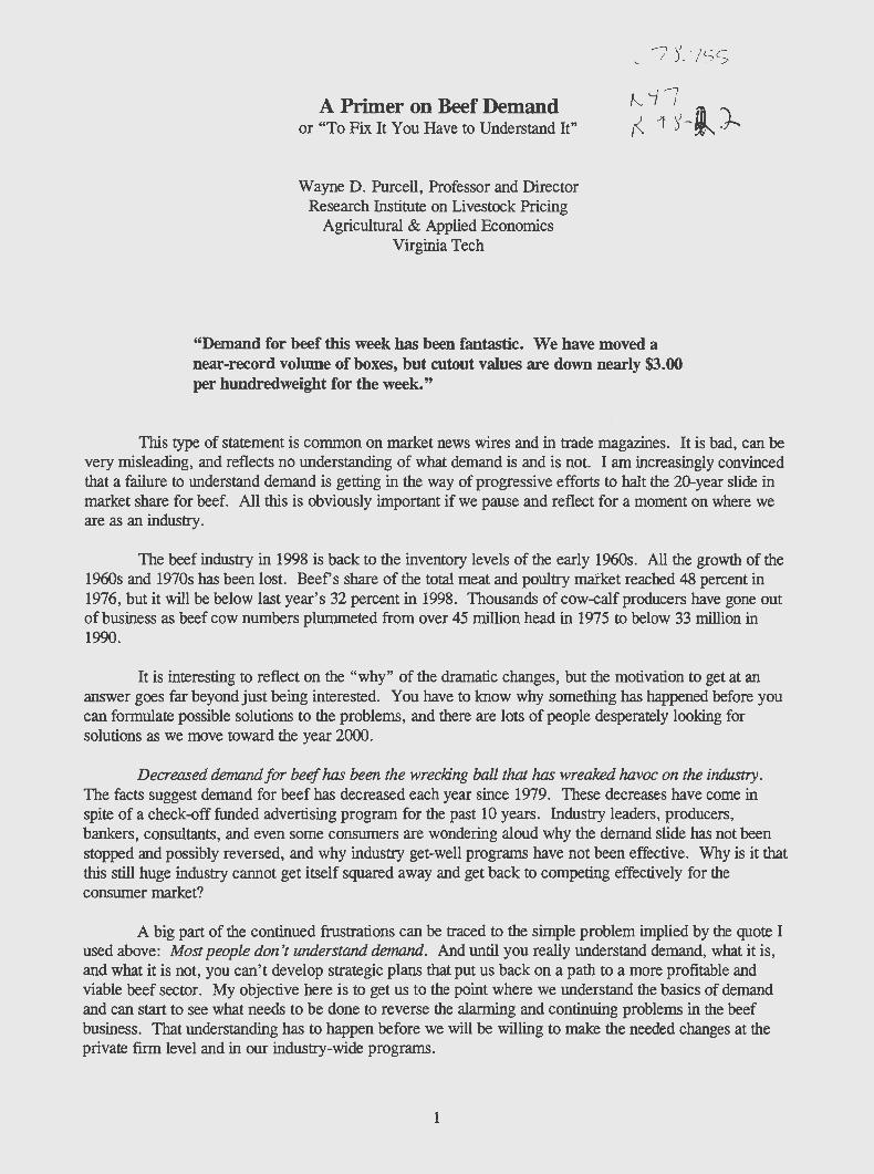
"Demand for beef this week has been fantastic. We have moved a near-record volume of boxes, but cutout values are down nearly $3.00 per hundredweight for the week."

This type of statement is common on market news wires and in trade magazines. It is bad, can be very misleading, and reflects no understanding of what demand is and is not. I am increasingly convinced that a failure to understand demand is getting in the way of progressive efforts to halt the 20-year slide in market share for beef. All this is obviously important if we pause and reflect for a moment on where we are as an industry.

The beef industry in 1998 is back to the inventory levels of the early 1960s. All the growth of the 1960s and 1970s has been lost. Beefs share of the total meat and poultry market reached 48 percent in 1976, but it will be below last year's 32 percent in 1998. Thousands of cow-calf producers have gone out of business as beef cow numbers plummeted from over 45 million head in 1975 to below 33 million in 1990.

It is interesting to reflect on the "why" of the dramatic changes, but the motivation to get at an answer goes far beyond just being interested. You have to know why something has happened before you can formulate possible solutions to the problems, and there are lots of people desperately looking for solutions as we move toward the year 2000.

Decreased demand for beef has been the wrecking ball that has wreaked havoc on the industry. The facts suggest demand for beef has decreased each year since 1979. These decreases have come in spite of a check-off funded advertising program for the past 10 years. Industry leaders, producers, bankers, consultants, and even some consumers are wondering aloud why the demand slide has not been stopped and possibly reversed, and why industry get-well programs have not been effective. Why is it that this still huge industry cannot get itself squared away and get back to competing effectively for the consumer market?

A big part of the continued frustrations can be traced to the simple problem implied by the quote I used above: Most people don't understand demand. And until you really understand demand, what it is, and what it is not, you can't develop strategic plans that put us back on a path to a more profitable and viable beef sector. My objective here is to get us to the point where we understand the basics of demand and can start to see what needs to be done to reverse the alarming and continuing problems in the beef business. That understanding has to happen before we will be willing to make the needed changes at the private firm level and in our industry-wide programs.

1

The Per-Capita Consumption Boondoggle, or What Demand is Not

To most cattlemen and even to some professionals who write about the beef business-and who ought to know better--per-capita consumption is seen as synonymous with demand. Nothing could be further from the truth. Making this mistake can lead you down all the wrong roads. Per-capita consumption is calculated by the USDA using an accounting approach to measure beginning beef stocks, production, and ending stocks. A "disappearance" measure is then generated and converted to a per-capita basis. If per-capita consumption measures anything directly, it measures per-capita supply. It certainly does not measure demand.

Figure 1 shows what sets the boundaries on per-capita consumption for any year. Per-capita supply, which becomes per-capita consumption, is closely related to January 1 total cattle inventories. We would expect that to be the case. Those inventory numbers set, within some relatively tight range, production or supply potential for the year. Per-capita consumption is thus largely pre-determined by prior management decisions that have determined January 1 inventory numbers. The years are shown in the plot. Note how per-capita consumption changes with the inventory numbers. A. simple regression model shows that January 1 inventories explain 80 percent of the year-to-year variation in per-capita supply. Per­capita consumption is clearly a supply measure.

140

130 74 ;5

• ;6

;3 J7 120 72

"0 82.. ~3 71 • .,8 «! ~ 4 • 0 Q)

65 831:~ ~76~9; ::I: 110

~ 9596 ~3 .s *64 6~5 100 9j ~41;7 ~ 7 86

~ 6 ~~. ~9 9~190

90

80

60 65 70 75 80 85 90 95 100

Per Capita Consumption

Figure 1. Total January 1 Cattle Inventories and Per-Capita Consumption of Beef, 1960-97

All this does not argue that per-capita consumption data are not useful. The plots in Figure 2 document the widely discussed loss of market share for beef. Per-capita consumption of beef, measured in retail weights, dropped some 30 pounds and over 30 percent from 1976 through 1997. It is apparent that chicken, measured in ready-to-cook weights, increased by more than 40 pounds and by more than 100 percent during the same period. On a per-capita basis, it is also clear the beef industry is getting smaller over time. But consumption data do not tell us why that decline is occurring. All they do is document the fact that resources and investments are flowing out of the beef industry. We need to deal with what is really causing per-capita consumption to decline-a drop in demand.

2

100

90

80

70 "' "'0 ~ 60 ::I 0 p..

50

40

30

20 0 \0 0\

C'l v \0 00 0 C'l v \0 00 0 C'l v \0 00 0 C'l v \0 \0 \0 \0 \0 t- t- t- t- t- 00 00 00 00 00 0\ 0\ 0\ 0\ 0\ 0\ 0\ 0\ 0\ 0\ 0\ 0\ 0\ 0\ 0\ 0\ 0\ 0\ 0\ 0\ 0\ 0\ - ..... ..... ..... ..... ..... ..... - - - .....

I-+-Beef ....,._Pork -Broilers I

Figure 2. Per-Capita Consumption of Beef, Pork, and Chicken, 1960-97

What Demand Really Is

Demand for any product or service is a schedule of the quantities consumers will take at various prices. Immediately, you can see both quantity and price are involved. And we know something about how those quantities and prices come together. Let's review an experience familiar to all of us.

Think about the last time you went shopping for a pair of shoes. You intend to buy one pair, but when you walk into the store, they have a big 50-percent price reduction sale going on. Do you ever walk out with two pairs when you intended to buy one pair? If you do, you buy two pairs for one simple reason: the price is lower.

You can reflect what is happening in a "law of demand":

At any point in time, consumers will take more quantity only at a lower price.

That means the demand line you could plot from a price-quantity schedule has a negative slope. It looks something like the curve labeled DD in Figure 3. (Actually, most demand curves will be convex to the horizontal axis and have a curvature, but Using straight lines is convenient and does not hurt our discussion at all.)

3

Price

D

D

Quantity

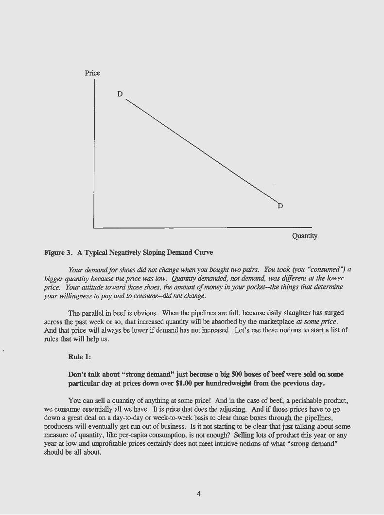
Figure 3. A Typical Negatively Sloping Demand Curve

Your demand for shoes did not change when you bought two pairs. You took (you "consumed") a bigger quantity because the price was low. Quantity demanded, not demand, was different at the lower price. Your attitude toward those shoes, the amozmt of money in your pocket--the things that determine your willingness to pay and to consume--did not change.

The parallel in beef is obvious. When the pipelines are full, because daily slaughter has surged across the past week or so, that increased quantity will be absorbed by the marketplace at some price. And that price will always be lower if demand has not increased. Let's use these notions to start a list of rules that will help us.

Rule 1:

Don't talk about "strong demand" just because a big 500 boxes of beef were sold on some particular day at prices down over $1.00 per hundredweight from the previous day.

You can sell a quantity of anything at some price! And in the case of beef, a perishable product, we consume essentially all we have. It is price that does the adjusting. And if those prices have to go down a great deal on a day-to-day or week-to-week basis to clear those boxes through the pipelines, producers will eventually get run out of business. Is it not starting to be clear that just talking about some measure of quantity, like per-capita consumption, is not enough? Selling lots of product this year or any year at low and unprofitable prices certainly does not meet intuitive notions of what "strong demand" should be all about.

4

Changes or Shifts in Demand: The Important Issue

We have found, then, that looking at quantity measures is not enough and can be misleading. Quantity demanded, which changes with price changes, is not demand. Demmui has not changed just because people consume more at lower prices. What, then, is a change in demand and why is it very important to lmow the difference?

Demand changes when the entire demmui curve shifts. This means consumers have changed the quantity they will buy at a particular price and, for that matter, at all possible prices. There are three primary shifters, three things that "shift" the curve: changes in consumer incomes, changes in prices of other (especially substitute) products, and changes in tastes and preferences. Let's look at each of these as we move toward an understanding of what is happening to beef demand, and why.

Generally, people want more of any product or service when their incomes go up. Beef is no exception. Higher income consumers, other things equal, tend to buy more beef, especially the higher priced cuts like steak. All my survey work shows that it is the higher income families who buy the steaks, but they also want-and are willing to pay for-quality, consistency, and convenience in preparation. Those same consumers are flocking to steakhouses (for an "eating out" experience), and they tend to go back to those restaurants where they get a really good cut of beef. Economists use something called income elasticity to measure how buying behavior in a particular product changes with changes in income. We know from research that there is a positive relationship between rising incomes and spending on beef.

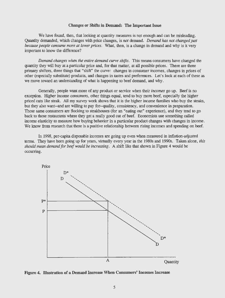
In 1998, per-capita disposable incomes are going up even when measured in inflation-adjusted terms. They have been going up for years, virtually every year in the 1980s and 1990s. Taken alone, this should mean demmui for beef would be increasing. A shift like that shown in Figure 4 would be occurring.

Price

D* D

P* 1-----------""""-"--+ ............

A

........ .......................

........ ................. ,

................................

........ ........

D

D*

Quantity

Figure 4. illustration of a Demand Increase When Consumers' Incomes Increase

5

A shift from DD to D*D* as incomes go up would mean a willingness to pay more for the same quantity, such as quantity A shown on the graph. Price for beef goes up from P to P*. But we know that is not happening. The 1997 price for beef, after adjustment for inflation to allow legitimate year-to-year comparisons, was at a record low, and 1997 per-capita consumption was below that of 1996. That is the opposite of what would be happening if rising consumer incomes were the only thing acting on beef demand.

It is starting to be obvious why knowing what is happening to demand is important. If demand is increasing, consumers are willing to pay higher prices for the same quantity. You want to invest in that type of business! But we don't have that pattern in beef, so another rule is in order.

Rule 2:

Something is wrong when consumer incomes are rising and beef prices are recording record low prices on a smaller per-capita offering.

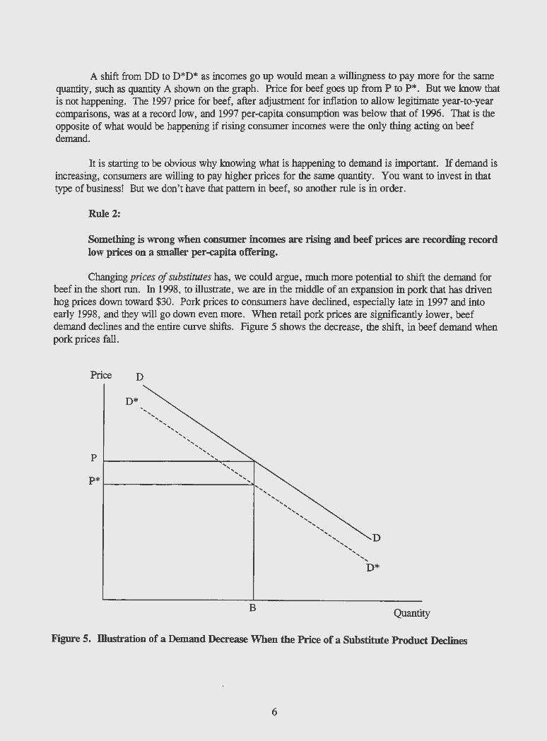
Changing prices of substitutes has, we could argue, much more potential to shift the demand for beef in the short run. In 1998, to illustrate, we are in the middle of an expansion in pork that has driven hog prices down toward $30. Pork prices to consumers have declined, especially late in 1997 and into early 1998, and they will go down even more. When retail pork prices are significantly lower, beef demand declines and the entire curve shifts. Figure 5 shows the decrease, the shift, in beef demand when pork prices fall.

Price D

D*

p

P*r---------------------~,

B

'',,,',,,

'',,,, ',

'',,,'',,, D

D*

Quantity

Figure 5. lliustration of a Demand Decrease When the Price of a Substitute Product Declines

6

A quantity of beef such as B would be taken only at lower prices, and this is consistent with the weak demand for beef during 1998. But during 1995 and 1996, the exact opposite was occurring. Retail pork prices were as low as $1.89 in June of 1995 and surged to as high as $2.34 in September of 1996. This should have increased beef demand, but as we will see later, beef demand showed no increase in 1996. It appears that pork prices are making weak beef demand worse, but the crossover effect from pork is not always strong enough to pull beef demand up--even when pork prices are surging.

But what about chicken? It is chicken, not pork, that most cattlemen point to when they talk about low-priced substitutes grabbing a bigger market share and taking the market away from beef. Coming into 1998, poultry production was up and chicken prices were slightly below year-earlier levels. But has it been cheap chicken that has pulled beef demand down across the years?

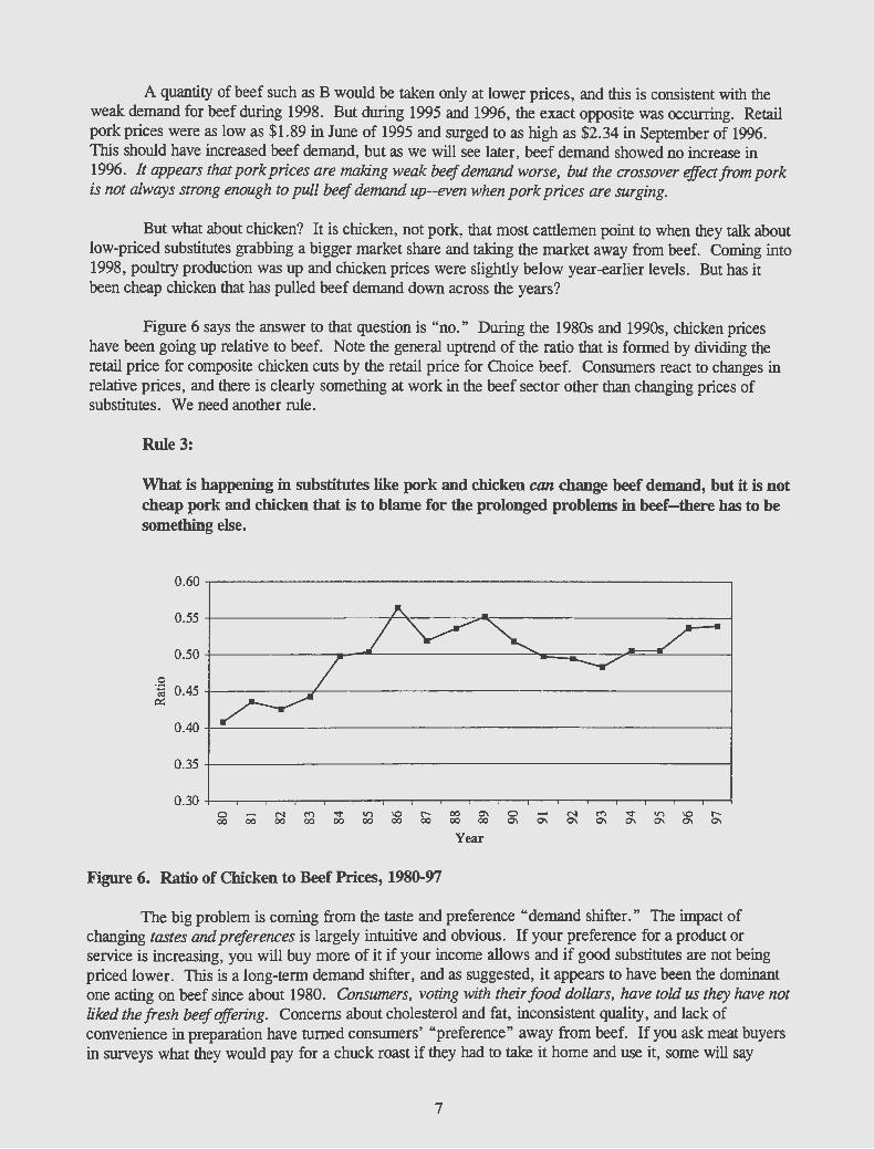
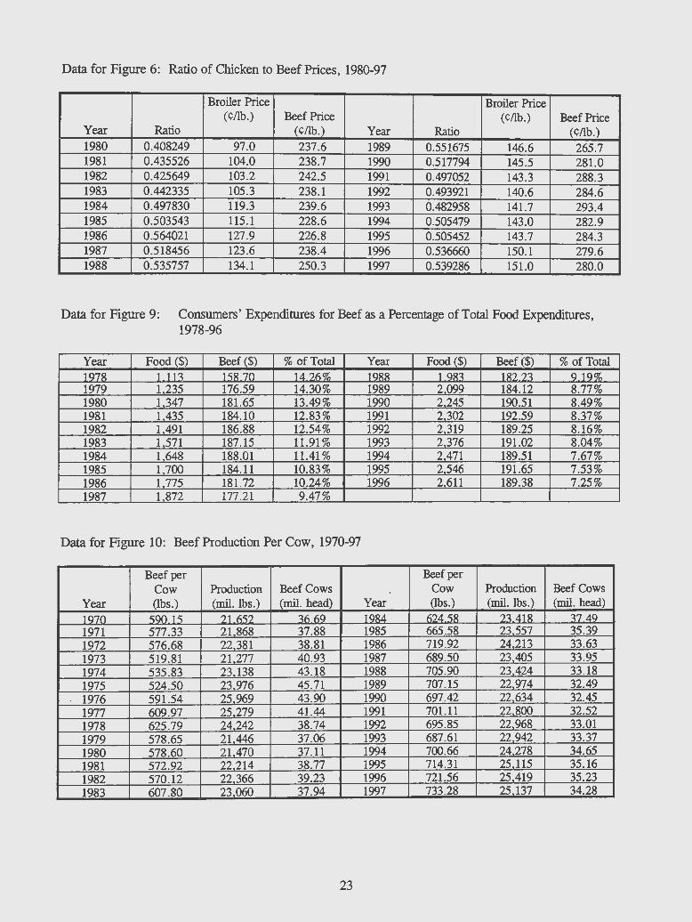
Figure 6 says the answer to that question is "no." During the 1980s and 1990s, chicken prices have been going up relative to beef. Note the general uptrend of the ratio that is formed by dividing the retail price for composite chicken cuts by the retail price for Choice beef. Consumers react to changes in relative prices, and there is clearly something at work in the beef sector other than changing prices of substitutes. We need another rule.

Rule 3:

What is happening in substitutes like pork and chicken can change beef demand, but it is not cheap pork and chicken that is to blame for the prolonged problems in beef-there has to be something else.

0.60

0.55

0.50

0 ·.:: "' 0.45 ~

0.40

0.35

Year

Figure 6. Ratio of Chicken to Beef Prices, 1980-97

The big problem is coming from the taste and preference "demand shifter." The impact of changing tastes and preferences is largely intuitive and obvious. If your preference for a product or service is increasing, you will buy more of it if your income allows and if good substitutes are not being priced lower. This is a long-term demand shifter, and as suggested, it appears to have been the dominant one acting on beef since about 1980. Consumers, voting with their food dollars, have told us they have not liked the fresh beef offering. Concerns about cholesterol and fat, inconsistent quality, and lack of convenience in preparation have turned consumers' "preference" away from beef. If you ask meat buyers in surveys what they would pay for a chuck roast if they bad to take it home and use it, some will say

7

"zero." This is especially likely for high-income families where all the adults are working outside the home ·and where everyone is in a rush and caught up in on-the-go lifestyles. But the chuck roast and the chuck steak are still about the only way the chuck is offered--unless it is ground and sold at bargain prices in the food store or in the burger businesses. We are not converting the chuck (or the round) to product forms the modem consumer wants, so another rule is in order.

Rule4:

If what you are offering is allowed to diverge from what a changing consumer wants, you will be in trouble, you can expect price declines-and something needs to be done before even more market share is lost.

Why Shifts in Demand are so Important

Before looking directly at the price-quantity data and the demand curves for beef, it is useful to pause, review, and emphasize why shifts in demand are so important to everyone in the beef industry. If the demand curve is stationary and not shifting, it should be clear by now that the only way you can sell more is at a lower price. For the beef or any other food sector to grow under these circumstances, you have to find cost-reducing technology and get the product produced cheaper. If demand is shifting down, the challenge to do it still cheaper and produce at still lower costs hits you hard--and continues to pound at you. If you can't do it cheaper and cheaper, you are out of business. Let's look at some examples.

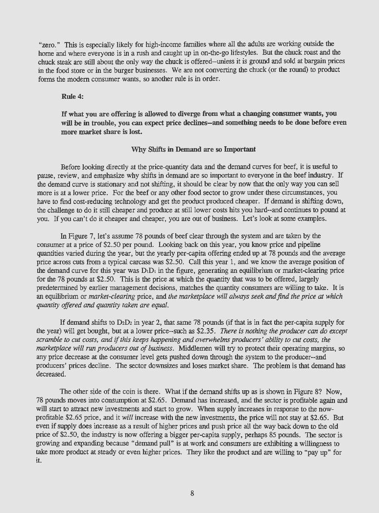
In Figure 7, let's assume 78 pounds of beef clear through the system and are taken by the consumer at a price of $2.50 per pound. Looking back on this year, you know price and pipeline quantities varied during the year, but the yearly per-capita offering ended up at 78 pounds and the average price across cuts from a typical carcass was $2.50. Call this year 1, and we know the average position of the demand curve for this year was DtDt in the figure, generating an equilibrium or market-clearing price for the 78 pounds at $2.50. Tills is the price at which the quantity that was to be offered, largely predetermined by earlier management decisions, matches the quantity consumers are willing to take. It is an equilibrium or market-clearing price, and the marketplace will always seek and find the price at which quantity offered and quantity taken are equal.

If demand shifts to D2D2 in year 2, that same 78 pounds (if that is in fact the per-capita supply for the year) will get bought, but at a lower price--such as $2.35. There is nothing the producer can do except scramble to cut costs, and if this keeps happening and overwhelms producers' ability to cut costs, the marketplace will run producers out of business. Middlemen will try to protect their operating margins, so any price decrease at the consumer level gets pushed down through the system to the producer-and producers' prices decline. The sector downsizes and loses market share. The problem is that demand has decreased.

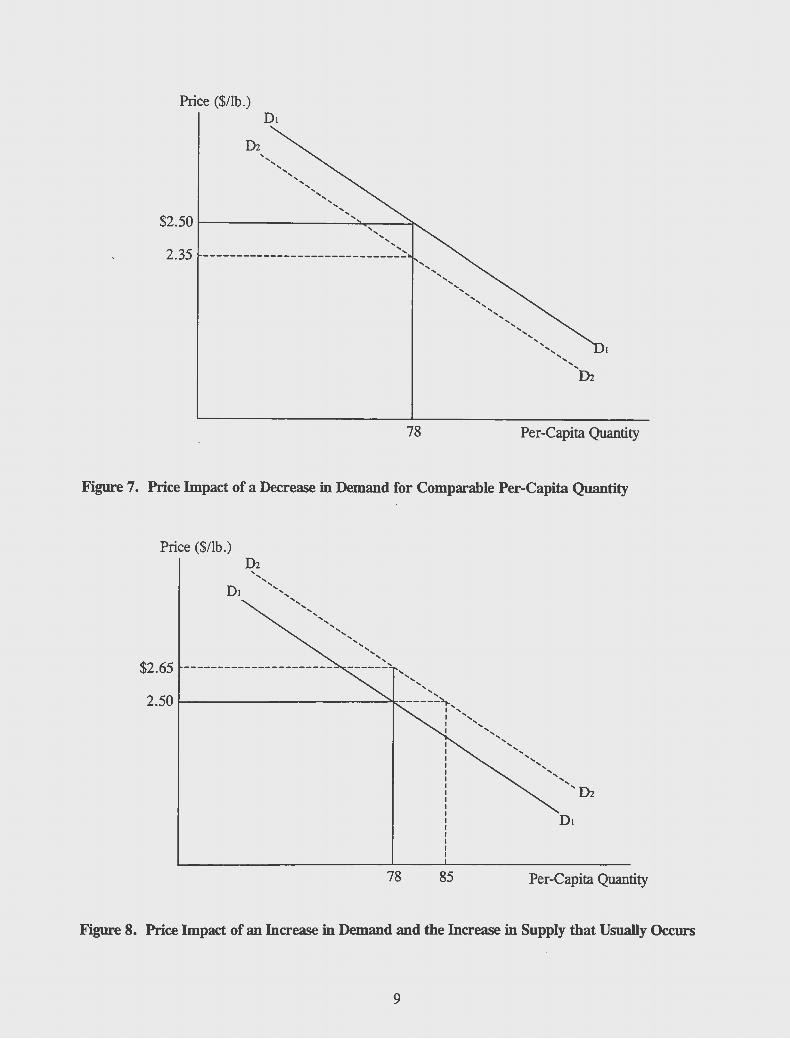
The other side of the coin is there. What if the demand shifts up as is shown in Figure 8? Now, 78 pounds moves into consumption at $2.65. Demand has increased, and the sector is profitable again and will start to attract new investments and start to grow. When supply increases in response to the now­profitable $2.65 price, and it will increase with the new investments, the price will not stay at $2.65. But even if supply does increase as a result of higher prices and push price all the way back down to the old price of $2.50, the industry is now offering a bigger per-capita supply, perhaps 85 pounds. The sector is growing and expanding because "demand pull" is at work and consumers are exhibiting a willingness to take more product at steady or even higher prices. They like the product and are willing to "pay up" for it.

8

Price ($/lb.)

78 Per-Capita Quantity

Figure 7. Price Impact of a Decrease in Demand for Comparable Per-Capita Quantity

Price ($/lb.)

' ' ',,

D• '',,,'',,,

...................

$2.65 ---------------------- ---~:~ ..... ........ ............

........ 2.50 1------------~------.......

I'-... I ', I ', I ' .... ,,

78 85

....... , .... ' .... ,

....... ....... 'In

Per-Capita Quantity

Figure 8. Price Impact of an Increase in Demand and the Increase in Supply that Usually Occurs

9

It is clear what situation we would all want. Demand increases, a shift in the entire demaiid curve up and to the right, will finance an expanding industry. Conswners' dollars are flowing into the business and becoming the catalyst for profits, new investments, growth, and change. This type of industry will not always be profitable for every producer, nor will it be profitable every year, but every increase in demand will bring a surge in profits, new investments, and a growing industry. ·

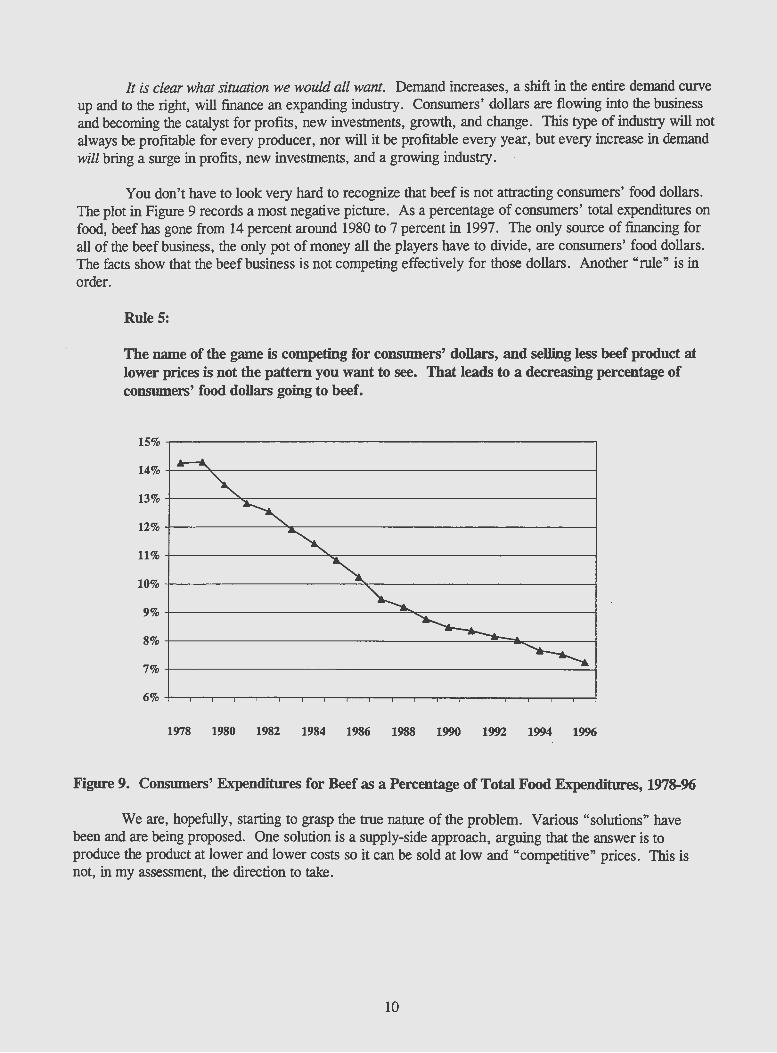
You don't have to look very hard to recognize that beef is not attracting consumers' food dollars. The plot in Figure 9 records a most negative picture. As a percentage of consumers' total expenditures on food, beef has gone from 14 percent around 1980 to 7 percent in 1997. The only source of financing for all of the beef business, the only pot of money all the players have to divide, are consumers' food dollars. The facts show that the beef business is not competing effectively for those dollars. Another "rule" is in order.

Rule 5:

The name of the game is competing for consumers' dollars, and selling less beef product at lower prices is not the pattern you want to see. That leads to a decreasing percentage of consumers' food dollars going to beef.

1978 1980 1982 1984 1986 1988 1990 1992 1994 1996

Figure 9. Consumers' Expenditures for Beef as a Percentage of Total Food Expenditures, 1978-96

We are, hopefully, starting to grasp the true nature of the problem. Various "solutions" have been and are being proposed. One solution is a supply-side approach, arguing that the answer is to produce the product at lower and lower costs so it can be sold at low and "competitive" prices. This is not, in my assessment, the direction to take.

10

The Cheap Product Solution

To this point, the facts suggest beef prices are working lower over time-and market share is declining. The demand curve at any point in time does slope down and to the right, and that has led, as suggested, to an often proposed "solution" --grow it cheaper and get prices to the conswner down to make beef more competitive in the retail store. A group of outside experts brought in by the National Cattlemen's Association (NCA) in the late 1980s proposed just such a solution.

There is some truth to this argument. You can be a bigger industry and hold more market share if you can get it done cheaper and move to a lower price/bigger quantity point on the demand curve. That might even work for a year or two if decreases in demand are not just driving the demand curve--and prices-still lower.

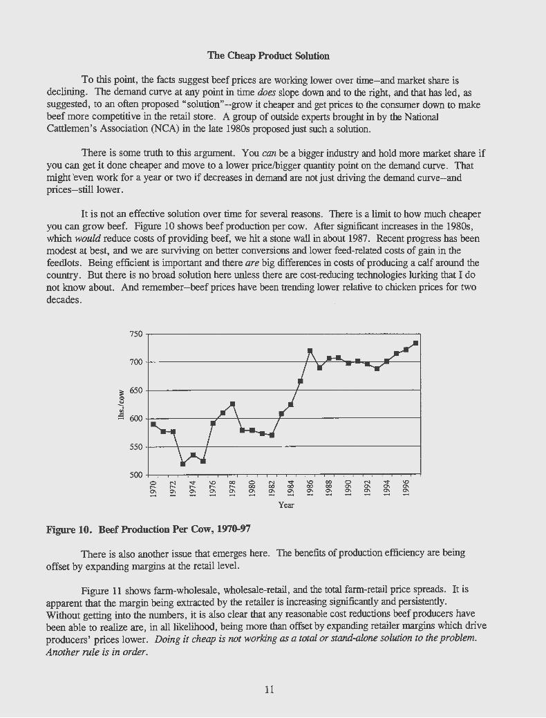
It is not an effective solution over time for several reasons. There is a limit to how much cheaper you can grow beef. Figure 10 shows beef production per cow. After significant increases in the 1980s, which would reduce costs of providing beef, we hit a stone wall in about 1987. Recent progress has been modest at best, and we are surviving on better conversions and lower feed-related costs of gain in the feedlots. Being efficient is important and there are big differences in costs of producing a calf around the country. But there is no broad solution here unless there are cost-reducing technologies lurking that I do not know about. And remember-beef prices have been trending lower relative to chicken prices for two decades.

~ 650+-----------------------+-------------------4 Q

~ .,; ~ 600+---------~~~------~--------------------~

500 0 N v \0 00 0 N v \0 00 0 N v \0 r-- r-- r-- r-- r-- 00 00 00 00 00 0\ 0\ 0\ 0\ 0\ 0\ 0\ 0\ 0\ 0\ 0\ 0\ 0\ 0\ 0\ 0\ 0\ 0\ ..... ..... - ..... ..... ..... ..... ..... ..... ..... ..... ..... .....

Year

Figure 10. Beef Production Per Cow, 1970-97

There is also another issue that emerges here. The benefits of production efficiency are being offset by expanding margins at the retail level.

Figure 11 shows farm-wholesale, wholesale-retail, and the total farm-retail price spreads. It is apparent that the margin being extracted by the retailer is increasing significantly and persistently. Without getting into the numbers, it is also clear that any reasonable cost reductions beef producers have been able to realize are, in all likelihood, being more than offset by expanding retailer margins which drive producers' prices lower. Doing it cheap is not working as a total or stand-alone solution to the problem. Another rule is in order.

11

Rule 6:

You can't build market share via low cost production and lower prices to consumers if there are limits to how much you can reduce costs and/or expanding middleman margins that just wipe out the benefits of your cost-reducing efforts.

160

140

120

100

~ 80 C) -... V'7

60

40

20

0 0 N r- r-

Farm-Wholesale

00 0 N '<t \0 oo 0 r- 00 00 00 00 00 0\

Year

Figure 11. Price Spreads for Beef, 1970-97

Turning to the Beef Data and Beef Demand

It's time to get at the facts, but before proceeding, let's recap what we have learned to this point:

• There is a big and important difference between quantity demmuled and demand. You can increase what any buyer will take, their "quantity demanded," if you reduce price. In particular, we learned (I trust) not to talk about "demand being strong" when in order to move quantity, you have to dramatically lower price.

• Per-capita consumption measures per-capita supply, not demand. If you produce more on a per-capita basis, you can be sure per-capita consumption will go up--but this does not say anything about demand. Price will go to whaJever level is needed to clear increased per-capita supplies through the pipelines. And unless demand is increasing, that increased per-capita offering means lower prices.

• It is shifts in demand, not just changes in quantity, thaJ will be a key to profitability. If demand is increasing and the entire demand curve is shifting up, consumers are willing to pay a higher price for the same quantity or for a larger quantity, and you are into a growth phase. There are enough consumer dollars being attracted to stimulate new investments and growth. Changes in incomes, relative prices, and changes in preferences can all do this-but the facts suggest demand for beef is decreasing, not increasing. When the curve shifts down, there is intolerable pressure on the producer --and some have to get out of business if demand continues to decrease and costs cannot be reduced enough to keep the business going.

12

• Decreases in spending on beef versus other foods is a symptom of problems, suggesting beef demand is declining. This means top-down pressure on prices starting with consumers' refusal to pay better prices for a product offering that has fallen out of favor. When consumer-level prices fall, the price pressure and lower prices go all the way down to the producer.

• Pressure back down toward the producer is even worse when middlemen's margins are expanding. Tiris appears to be especially true at the retail level where price spreads for beef are expanding, suggesting increased costs, bigger profit margins, or some combination of the two.

• Indirectly, we have covered another important point. You cannot include beef price when listing reasons for weak beef demand. Specifically, you cannot say demand for beef is weak because of "high beef prices. " Price is part of the demand schedule, the set of price-quantity combinations, for beef-it cannot be a "demand shifter." Analysts and observers who use beef price in this way are really talking about the importance of price in determining quantity demanded, and we have learned that per-capita supplies or any other measure of quantity is not a correct measure of demand.

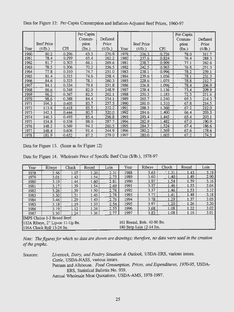
With these points in mind, it's time to get to the specifics. The facts about beef can be presented in several ways. A useful overall picture is shown in Figure 12 with per-capita consumption and inflation­adjusted beef prices shown as line plots. The general pattern since the late 1970s shows price and per­capita consumption trending down. Overall, that means offering and selling less product at lower prices, and you don't have to spend years studying economics to recognize that pattern means something is badly wrong on the demand side of the price equation. (You will find these data at the end of the manuscript if you want to see the numbers or work with them in some way.)

Figure 12.

330~-------------------------------------------.

310

290

~ 270

~ 250 5 u ~ 230 u

;t 210

190

170

150~~~~-.0T~-r~TO~>OTOoo-r~TO~>OTO~roo+

1-Deflated Price __.Per Capita Consumption I

100

95 ,.-... .,;

90 .0 ::::-c

85 0 ·.::: "'" 80 8 ::1

"' c 75 0 u 70 5 ·s.

"' 65 u .!. CLl

60 A.

55

Per-Capita Consumption and Inflation-Adjusted Beef Prices (CPI, 1982-84=100), 1960-97

Before looking at the data a second way, let's pause and review why the influence of price inflation has to be removed from the beef prices. To legitimately compare years, you want the price changes to be due to the economics of supply and demand, not just because all price levels are changing over time. If it is both price inflation and supply/demand forces that are moving prices, you cannot tell which part of the price change is due to price inflation and which part is due to shifts in supply and/or

13

demand. Dividing the prices by the Copsumer Price Index (CPI, 1982-84= 100) converts all the prices to a common denominator (to 1982-84 dollars) by removing the influence of inflation. It removes the price inflation influence and lets us focus on what the supply-demand balance is doing. After this is done, you can compare years and learn something useful.

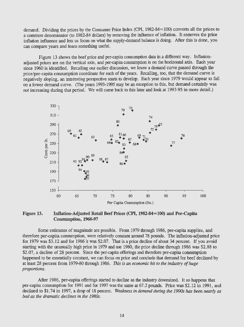
Figure 13 shows the beef price and per-capita consumption data in a different way. Inflation­adjusted prices are on the vertical axis, and per-capita consumption is on the horizontal axis. Each year since 1960 is identified. Recalling our earlier discussion, we lmow a demand curve passed through the price/per-capita consumption coordinate for each of the years. Recalling, too, that the demand curve is negatively sloping, an interesting perspective starts to develop. Each year since 1979 would appear to fall on a lower demand curve. (The years 1993-1995 may be an exception to this, but demand certainly was not increasing during that period. We will come back to this later and look at 1993-95 in more detail.)

Figure 13.

330

310

290

270 ~

-: 250 C1.l c.. "' 5 230

C)

210

190

170

60 62 • 61.. 63

90 89

93 929~· •

•• 94 ·.?5

J~

•

79 7~

• 74 80 • • 78.5

n• 65 8166 ~ 71 • • • • 67 ·~0

6# 8z. 83 • 68•

• 8~

85

• 86•

77 • 76 •

150+------.-----.----~,-----~----.-----~-----.----~

60 65 70 75 80 85 90 95

Per Capita Consumption (lbs.)

Inflation-Adjusted Retail Beef Prices (CPI, 1982-84=100) and Per-Capita Consumption, 1960-97

100

Some estimates of magnirude are possible. From 1979 through 1986, per-capita supplies, and therefore per-capita consumption, were relatively constant around 78 pounds. The inflation-adjusted price for 1979 was $3 .12 and for 1986 it was $2.07. That is a price decline of about 34 percent. If you avoid starting with the unusually high price in 1979 and use 1980, the price decline through 1986 was $2.88 to $2.07, a decline of 28 percent. Since the per -capita offerings and therefore per -capita consumption happened to be essentially constant, we can focus on price and conclude that demand for beef declined by at least 28 percent from 1979-80 through 1986. This is an economic hit to the industry of huge proponions.

After 1986, per-capita offerings started to decline as the industry downsized. It so happens that per-capita consumption for 1991 and for 1997 was the same at 67.2 pounds. Price was $2.12 in 1991, and declined to $1.74 in 1997, a drop of 18 percent. Weakness in demand during the 1990s has been nearly as bad as the dramatic declines in the 1980s.

14

In the face of this dramatic evidence, there has still been a longstanding tendency for producers and producer groups to refuse to accept that they have a problem. In the late 1980s, the National Livestock and Meat Board (NLMB) organized "demand strategy" conferences during the national summer meetings. Attention was focused on the growing demand problems and on what needed to be done to help correct the situation. There were even signs that NLMB staff, mostly trained in the physical sciences, were starting to understand what demand is and is not. Was there a light at the end of the tunnel? Would this growing awareness lead to progressive industry programs to do something about demand?

Within two to three years, however, the producer community and producer leaders started to complain about the time the demand strategy conferences were taking and about what it cost to organize and conduct a conference. It was taking time from their important committee work, cost too much, and they were getting tired of "having these agricultural economists coming to the conferences and talking about demand problems with the product." They could not and would not accept the fact consumers were finding fault with their beloved product. Obviously, a rule can be pulled from this.

Rule 7:

Don't ignore the facts on demand just because you don't like the message they are delivering.

Part of the problem may be in our failure to help producers and their elected leaders understand what it all means. They often sense there is a problem because they know they are periodically in a cost­price squeeze, but it is sometimes hard to make that connection all the way up to what consumers are doing. What, exactly, does all this mean to the cattle producer? With that issue in mind, let's try to "put some numbers" on it.

The 1991 to 1997 comparison is straightforward. In 1991, the average nominal price-before adjusting for inflation-was $2.88 per pound. From 1991 through 1997, the overall price level as measured by the CPI increased by 18 percent. If 1997 had been on the same demand curve as 1991, the 1997nominal price would have been near 1.18 ($2.88) = $3.40 just due to price inflation. With a $2.88 retail price in 1991, Cattle Fax reported an average fed steer price of $74.28. If the price spreads in 1997 were the same relative to retail prices, a 1997 fed steer price can be calculated assuming demand was the same in 1997 as in 1991 and the $2.80 price had just "inflated" up to $3.40.

$2.88 $3.40 =

$74.28 X

X= $87.69

With constant demand from 1991 through 1997, inflation would have boosted fed cattle prices to $87.69 in 1997.

The actual fed cattle price in 1997 was $66.10, over $20 per hundredweight below the "derived" price of $87.69. This is obviously huge in terms of impact on producers and on the industry. Lower fed cattle prices translate directly to lower feeder cattle and calf prices. Producers get pushed out of business and inventory numbers decline.

Price spreads can also make a difference. The farm-to-retail price spread did not increase as fast as price inflation, increasing by only 11 percent between 1991 and 1997. (Recall that the CPI increased

15

18 percent.) Those smaller price spread increases would have contributed to a still bigger price increase for cattle, and it might have been above $87.69 if demand in 1997 had been at 1991levels. But let's keep things simple and use the $87.69. It was demand problems that brought price down to $66.10 compared to the "could have been" price of $87.69.

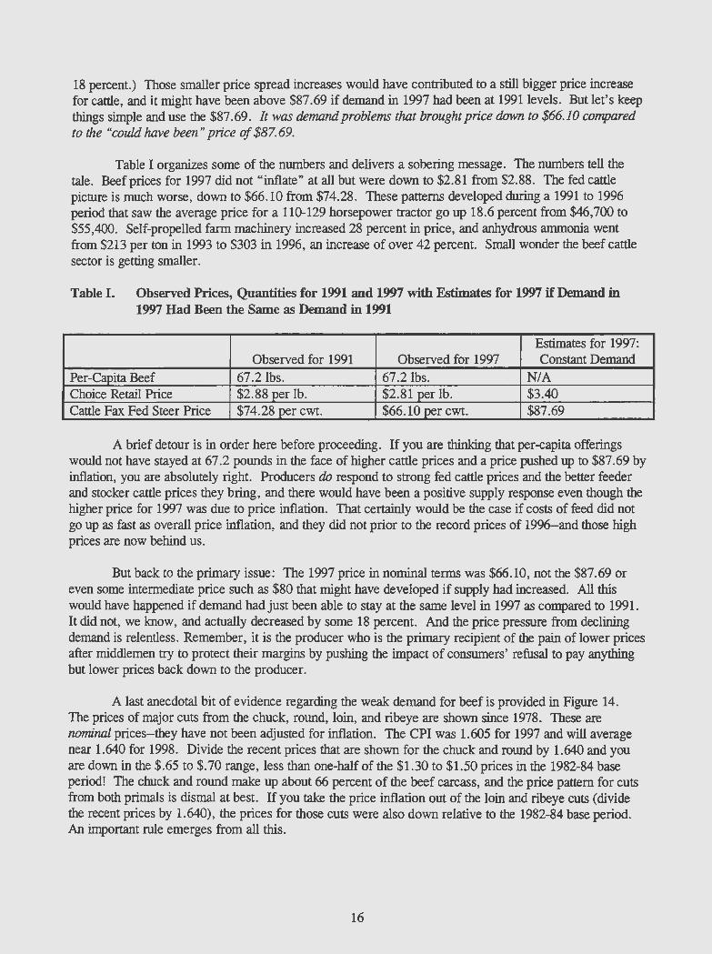
Table I organizes some of the numbers and delivers a sobering message. The numbers tell the tale. Beef prices for 1997 did not "inflate" at all but were down to $2.81 from $2.88. The fed cattle picture is much worse, down to $66.10 from $74.28. These patterns developed during a 1991 to 1996 period that saw the average price for a 110-129 horsepower tractor go up 18.6 percent from $46,700 to $55,400. Self-propelled farm machinery increased 28 percent in price, and anhydrous ammonia went from $213 per ton in 1993 to $303 in 1996, an increase of over 42 percent. Small wonder the beef cattle sector is getting smaller.

Table I. Observed Prices, Quantities for 1991 and 1997 with Estimates for 1997 if Demand in 1997 Had Been the Same as Demand in 1991

Estimates for 1997: Observed for 1991 Observed for 1997 Constant Demand

Per-Capita Beef 67.2lbs. 67.2lbs. N/A Choice Retail Price $2.88 per lb. $2.81 per lb. $3.40 Cattle Fax Fed Steer Price $74.28 per cwt. $66.10 per cwt. $87.69

A brief detour is in order here before proceeding. If you are thinking that per-capita offerings would not have stayed at 67.2 pounds in the face of higher cattle prices and a price pushed up to $87.69 by inflation, you are absolutely right. Producers do respond to strong fed cattle prices and the better feeder and stocker cattle prices they bring, and there would have been a positive supply response even though the higher price for 1997 was due to price inflation. That certainly would be the case if costs of feed did not go up as fast as overall price inflation, and they did not prior to the record prices of 1996-and those high prices are now behind us.

But back to the primary issue: The 1997 price in nominal terms was $66.10, not the $87.69 or even some intermediate price such as $80 that might have developed if supply had increased. All this would have happened if demand had just been able to stay at the same level in 1997 as compared to 1991. It did not, we know, and actually decreased by some 18 percent. And the price pressure from declining demand is relentless. Remember, it is the producer who is the primary recipient of the pain of lower prices after middlemen try to protect their margins by pushing the impact of consumers' refusal to pay anything but lower prices back down to the producer.

A last anecdotal bit of evidence regarding the weak demand for beef is provided in Figure 14. The prices of major cuts from the chuck, round, loin, and ribeye are shown since 1978. These are nominal prices-they have not been adjusted for inflation. The CPI was 1.605 for 1997 and will average near 1.640 for 1998. Divide the recent prices that are shown for the chuck and round by 1.640 and you are down in the $.65 to $.70 range, less than one-half of the $1.30 to $1.50 prices in the 1982-84 base period! The chuck and round make up about 66 percent of the beef carcass, and the price pattern for cuts from both primals is dismal at best. If you take the price inflation out of the loin and ribeye cuts (divide the recent prices by 1.640), the prices for those cuts were also down relative to the 1982-84 base period. An important rule emerges from all this.

16

Rule 8:

You cannot ignore the message being sent by consumers when they will take smaller quantities of your product only at lower prices over time. That price pressure prompts the marketplace to look for a new market clearing price for cattle, and the only way the marketplace has of restoring a balance is to decrease supply and drive resources-and people-out of the beef business.

4.50 ,------------------------------.

4.00 +-------------------------------1

3.50 +-------------~=---:.!!!!..._ _ __.JR=::IL. ______ --1

3.oo +----~~~~---~~~----.~~~~-==:!:~::::::.c~----J

@ 2.50~~-------~~~--------------~ &'3-

2.00+--------------------------~

1.50 !~~==:=~=~:;~~~~=:=~~::~~~~~;j 1.00

0.50 +---.----..-...---r---r-.----r---.---,.---.----.--.---..---...--.----.---.--.-----,...---l

1--Ribeye __.__Chuck -+-Round -Loin I

Figure 14. Wholesale Price of Specific Beef Cuts, 1978-97

Demand appears to be the key issue. It is not a supply issue. Resources have left beef, and some of those resources have moved into production of other food products--including pork and poultry. To the extent that poultry, for example, has been more profitable based strictly on efficiencies in production, we could argue that there is a supply-side instrument of change to all this--and there clearly is. But the dominant economic hit has come from the runaway train that is the lower and lower beef prices, prices so low they have destroyed profitability for many cattlemen. Demand has to get more attention, but before trying to pull the key messages from all this together, let's state another rule.

Rule 9:

You must be capable of analyzing price/quantity data and be able to determine what is happening to demand from one time period to the next.

Procedures to be followed are not difficult. There are two basic approaches. For both approaches, you must adjust the price data for price inflation. You do that by dividing your prices by the consumer price index, and the current CPI the government uses sets 1982-84 as the base period. To illustrate, the average price at retail for Choice beef, the CPI, and inflation-adjusted prices are shown here for 1990-1997 (all data are at the end of the manuscript, remember):

17

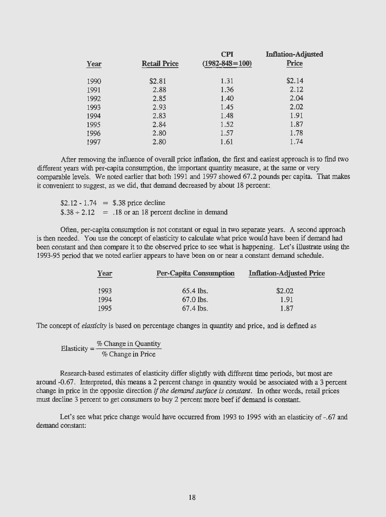
CPI Inflation-Adjusted Year Retail Price (1982-848 = 100) Price

1990 $2.81 1.31 $2.14 1991 2.88 1.36 2.12 1992 2.85 1.40 2.04 1993 2.93 1.45 2.02 1994 2.83 1.48 1.91 1995 2.84 1.52 1.87 1996 2.80 1.57 1.78 1997 2.80 1.61 1.74

After removing the influence of overall price inflation, the first and easiest approach is to find two different years with per-capita consumption, the important quantity measure, at the same or very comparable levels. We noted earlier that both 1991 and 1997 showed 67.2 pounds per capita. 1bat makes it convenient to suggest, as we did, that demand decreased by about 18 percent:.

$2.12- 1. 74 = $.38 price decline $.38 + 2.12 = .18 or an 18 percent decline in demand

Often, per-capita consumption is not constant or equal in two separate years. A second approach is then needed. You use the concept of elasticity to calculate what price would have been if demand had been constant and then compare it to the observed price to see what is happening. Let's illustrate using the 1993-95 period that we noted earlier appears to have been on or near a constant demand schedule.

Year

1993 1994 1995

Per-Capita Consumption

65.4lbs. 67.0 lbs. 67.4lbs.

Inflation-Adjusted Price

$2.02 1.91 1.87

The concept of elastidty is based on percentage changes in quantity and price, and is defined as

El . . % Change in Quantity

astlctty = -----"'----'--~ % Change in Price

Research-based estimates of elasticity differ slightly with different time periods, but most are around -0.67. Interpreted, this means a 2 percent change in quantity would be associated with a 3 percent change in price in the opposite direction if the demand surface is constant. In other words, retail prices must decline 3 percent to get consumers to buy 2 percent more beef if demand is constant.

Let' s see what price change would have occurred from 1993 to 1995 with an elasticity of -.67 and demand constant:

18

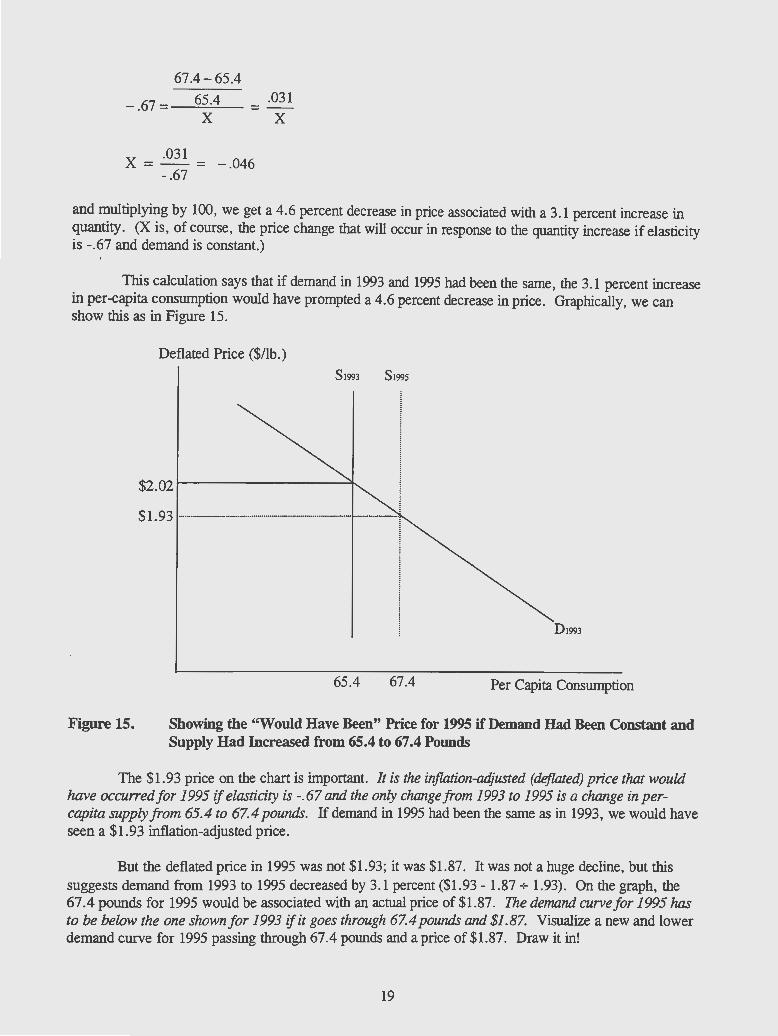
67.4-65.4

-.67=-....::.6=5 . ...:...4_- _.03_1 X X

X = ·031

= -.046 -.67

and multiplying by 100, we get a 4.6 percent decrease in price associated with a 3.1 percent increase in quantity. (X is, of course, the price change that will occur in response to the quantity increase if elasticity is -.67 and demand is constant.)

This calculation says that if demand in 1993 and 1995 had been the same, the 3.1 percent increase in per-capita consumption would have prompted a 4.6 percent decrease in price. Graphically, we can show this as in Figure 15.

Figure 15.

Deflated Price ($/lb.)

S1993 S199s

$2.021----------~

$1.93 -·-·-·-·-·-····-····--·----·- +--

65.4 67.4

01993

Per Capita Consumption

Showing the "Would Have Been" Price for 1995 if Demand Had Been Constant and Supply Had Increased from 65.4 to 67.4 Pounds

The $1.93 price on the chart is important. It is the inflation-adjusted (deflated) price that would have occurred for 1995 if elastidty is -.67 and the only change from 1993 to 1995 is a change in per­capita supply from 65.4 to 67.4 pounds. If demand in 1995 had been the same as in 1993, we would have seen a $1.93 inflation-adjusted price.

But the deflated price in 1995 was not $1.93; it was $1.87. It was not a huge decline, but this suggests demand from 1993 to 1995 decreased by 3.1 percent ($1.93- 1.87 + 1.93). On the graph, the 67.4 pounds for 1995 would be associated with an actual price of $1.87. The demand curve for 1995 has to be below the one shown for 1993 if it goes through 67.4 pounds and $1.87. Visualize a new and lower demand curve for 1995 passing through 67.4 pounds and a price of $1.87. Draw it in!

19

It's worth some effort and a bit of digging. If demand is increasing, the sector can grow. Consumers' are paying prices high enough (because they like the product(s)) to bring periodic profits, stimulate new investments, and prompt a growth sector. If demand is going in the opposite direction, as it is in beef, the converse of all these responses occurs. Producers can't make a profit, investments flow out as they go out of business, and the sector downsizes c:nd loses market share.

Tills exercise is about a primer on demand, but I would be remiss if I did not share my perceptions of why beef demand has decreased over a long time period. At several points, I have noted that the facts suggest consumers are not liking what they are being offered in the fresh beef counter. (There are comparable if less severe problems in the restaurant and institution businesses.) In specific terms, the survey and research evidence suggests the modem consumer want

• Low-fat and low-cholesterol products; • High quality products that offer a favorable eating experience; • Products that offer that positive eating experience consistently and reliably; and • Products and product forms that are convenient and easy to prepare.

All this suggests that before we buy into "changing the genetics" as a proposed solution for the industry, something needs to be done about changing the offering of fresh beef. The genetic solution will take a long time, and there is no reason to wait to start correcting the demand problems. Turning what we are now producing into low-fat, tasty, and convenient eating experiences will help revitalize the industry while we are working on the genetics.

Product development work costs money, but it has to get done. This year, the new National Cattlemen's Beef Association (NCB A) offered a prize for the best new beef product developed during the past year. The award was $250,000, a step in the right direction. But the NCBA (and prior NCA/NLMB) committees have voted for some $25-35 million in check-off dollars to be spent on generic advertising, communication, etc., each year since the late 1980s. But those programs have questionable impact, perhaps because our meat scientist colleagues now agree that the product failure rate for Choice beef cuts is around 20 percent. We must change the product offering to clean up the quality problems and reduce that product failure rate.

We will not fix the problems with the product, however, until we have broad recognition that we have major problems. But as I noted in the beginning, we can't get positioned to fix demand problems until we understand what demand is and is not. I hope this brief treatise has helped get us all on the right track with a better understanding of what needs to be done. Let me close by reviewing the important "rules" of this paper.

• Per-capita consumption is not a measure of demand. • Talking about "strong demand" when increased quantities are being taken at sharply lower prices is

wrong and misleading. • If demand is constant, the only way an increased per-capita supply will be taken by consumers is at

lower prices. • You cannot use high beef prices as a reason for weak beef demand since price is part of the demand

schedule. • If demand is decreasing, the only way to avoid losing market share is to reduce costs enough to keep

the business viable.

20

• A prolonged period of decreasing demand for beef will eventually exceed even the most efficient producer's ability to cut costs.

• Significant changes in pork and chicken prices can and will shift beef demand from year to year and within the year.

• Changes in consumers' incomes are usually positive for beef demand, but rising incomes during the 1980s and 1990s have not offset other problems.

• The facts support a conclusion that, since 1979-80, consumers' preferences have turned away from beef as their needs and lifestyles have changed.

• If these pervasive problems are not fixed and the negative trend in beef demand isn' t at least stopped, the beef sector will lose market share and will trend toward a smaller industry for the foreseeable future.

• It is time to do something, time to understand, time to get the product offering moved toward what the modem consumer wants and is willing to pay for.

The beef business was a growth sector during the 1906s and most of the 1970s. Consumers were developing a taste for marbled beef. Demand increased, and profit potential pulled new investments into the industry; Around 1979, consumers' attitudes started to change--but the product offering did not change. That divergence between what consumers want and are willing to pay for has continued to grow, and the industry has been forced into a pattern of disinvestment and downsizing. We will not find the investments and the programs that will be needed to correct these long-standing problems until we fully understand demand, what decreases in demand are and why they have occurred, and what will be required to reverse this disastrous trend and prompt increases in demand at the consumer level.

21

Appendix - Data Used to Graph Figures

Data for Figure 1: Total January 1 Cattle Inventories and Per-Capita Consumption of Beef, 1960-97

Total Cattle Per-Capita Beef Total Cattle Per-Capita Beef Inventory Consumption Inventory Consumption

Year (mil. head) (lbs.) Year (mil. head) (lbs.) 19no 9n.2 63.3 1979 110.9 78.0 1961 97.7 65.4 1980 111.2 76.4 1962 100.4 66.1 1981 114.4 77.1 1963 104.5 70.2 1982 115.4 76.8 1964 107.9 74.7 1983 115.0 78.2 1965 109.0 74.6 1984 113.4 78.1 1966 108.9 78.1 1985 109.6 78.8 1967 108.8 79.8 1986 105.4 78.4 1968 109.4 82.0 1987 102.1 73.4 1969 110.0 82.5 1988 99.6 72.3 1970 112.4 84.4 1989 96.7 69.3 1971 114.6 83.7 1990 .95.8 67.8 1972 117.9 85.5 1991 96.4 67.2 1973 121.5 80.5 1992 97.6 66.4 1974 127.8 85.4 1993 99.2 65.4 1975 132.0 88.0 1994 101.0 67.0 1976 128.0 94.2 1995 102.8 67.4 1977 122.8 91.4 1996 103.8 67.6 1978 116.4 87.2 1997 101.2 67.2

Data for Figure 2: Per-Capita Consumption (lbs.) of Beef, Pork, and Chicken, 1960-97

Year Beef Pork Broilers Year Beef Pork Broilers 1960 63.3 59~84 23.4 1979 78.0 52.89 47.4 1961 65.4 55.05 26.0 1980 76.4 56.44 46.7 1962 66.1 57.82 25.8 1981 77.1 53.73 48.2 1963 70.2 58.83 27.1 1982 76.8 48.11 49.6 1964 74.7 58.74 27.7 1983 78.2 50.66 50.4 1965 74.6 52.12 29.6 1984 78.1 50.28 52.6 1966 78.1 50.80 31.9 1985 78.8 50.65 55.1 1967 79.8 55.60 32.3 1986 78.4 47.82 56.3 1968 82.0 56.75 32.6 1987 73.4 48.12 60.2 1969 82.5 54.98 34.6 1988 72.3 51.73 62.5 1970 84.4 55.90 36.5 1989 69.3 51.57 66.3 1971 83 .7 60.44 36.3 1990 67.8 49.35 69.2 1972 85.5 54.42 37.9 1991 67.2 50.5 72.6 1973 80.5 48.65 36.9 1992 66.4 53.2 75.9 1974 85.4 52.57 36.9 1993 65.4 52.3 78.0 1975 88.0 42.58 36.5 1994 67.0 53.1 79.3 1976 94.2 45.34 39.6 1995 67.4 52.4 79.2 1977 91.4 46.57 40.8 1996 67.6 49.1 81.4 1978 87.2 46.43 43 .5 1997 67.2 48.0 83.7

22

Data for Figure 6: Ratio of Chicken to Beef Prices, 1980-97

Broiler Price Broiler Price (C!lb.) Beef Price (C/lb.) Beef Price

Year Ratio (C!lb.) Year Ratio (Cilb.) 1980 0.408249 97.0 237.6 1989 0.551675 146.6 265.7 1981 0.435526 104.0 238.7 1990 0.517794 145.5 281.0 1982 0.425649 103.2 242.5 1991 0.497052 143.3 288.3 1983 0.442335 105.3 238.1 1992 0.493921 140.6 284.6 1984 0.497830 119.3 239.6 1993 0.482958 141.7 293.4 1985 0.503543 115.1 228.6 1994 0.505479 143.0 282.9 1986 0.564021 127.9 226.8 1995 0.505452 143.7 284.3 1987 0.518456 123.6 238.4 1996 0.536660 150.1 279.6 1988 0.535757 134.1 250.3 1997 0.539286 151.0 280.0

Data for Figure 9: Consumers' Expenditures for Beef as a Percentage of Total Food Expenditures, 1978-96 '

Year Food($) Beef($) % ofTotal Year Food($) Beef($) %of Total 1978 1 1 n 1 ')R .70 14 2(}% 19RR 1.9R1 1R2.21 9.19% 1979 1.235 176.59 14.30% 1989 2 099 184.12 8.77% 1980 1 347 181.65 13.49% 1990 2 245 190.51 8.49% 1981 1 435 184.10 12.83% 1991 2 302 192.59 8.37% 1982 1 491 186.88 12.54% 1992 2 319 189.25 8.16% 1983 1 571 187.15 11.91% 1993 2 376 191.02 8.04% 1984 1 648 188.01 11.41% 1994 2 471 189.51 7.67% 1985 1 700 184.11 10.83% 1995 2 546 191.65 7.53% 1986 1 775 181.72 10.24% 1996 2611 189.38 7.25% 1987 1 872 177.21 9.47%

Data for Figure 10: Beef Production Per Cow, 1970-97

Beef per Beef per Cow Production Beef Cows Cow Production Beef Cows

Year (lbs.) (mil. lbs.) (mil. head) Year (lbs.) (mil. lbs.) (mil. head)

1970 590.15 21.652 1n n9 19&4 624.58 23.418 37.49 1971 577.33 21 868 37.88 1985 665.58 23 557 35.39 1972 576.68 22 381 38.81 1986 719.92 24 213 33.63 1973 519.81 21277 40.93 1987 689.50 23 405 33.95 1974 535.83 23 138 43.18 1988 705.90 23 424 33.18 1975 524.50 23 976 45.71 1989 707.15 22 974 32.49 1976 591.54 25 969 43.90 1990 697.42 22 634 32.45 1977 609.97 25 279 41.44 1991 701.11 22 800 32.52 1978 625.79 24 242 38.74 1992 695.85 22 968 33.01 1979 578.65 21 446 37.06 1993 687.61 22 942 33.37 1980 578.60 21470 37.11 1994 700.66 24 278 34.65 1981 572.92 22 214 38.77 1995 714.31 25 115 35.16 1982 570.12 22 366 39.23 1996 721.56 25 419 35.23 1983 607.80 23 060 37.94 1997 733 .28 25 137 34.28

23

Data for Figure 11: Price Spreads for Beef ($/cwt.), 1970-97

Year Net Farm Value Retail Price Farm-Retail Farm-Wholesale Wholesale-Retail 1970 64.2 99.9 357 12_6 211 1971 70.7 106.2 35.5 14.4 21.1 1972 76.0 116.6 40.6 14.3 26.4 1973 94.7 139.7 45.0 16.1 28.9 1974 91.8 143.8 52.0 18.4 33.7 1975 99.4 152.2 52.8 19.8 33.0 1976 84.4 145.7 61.3 16.2 45.0 1977 86.0 145.8 59.8 17.3 42.6 1978 111.7 178.8 67.1 19.7 47.4 1979 141.7 222.4 80.7 24.1 56.7 1980 145.7 233.6 87.9 25.4 62.5 1981 139.1 234.7 95.6 25.2 70.3 1982 141.1 238.4 97.3 24.8 72.4 1983 136.8 234.1 97.3 23.3 74.0 1984 140.7 235.5 94.8 21.7 72.9 1985 127.4 228.6 101.2 21.3 79.8 1986 125.0 226.8 101.8 21.5' 80.2 1987 138.7 238.4 99.7 21.3 78.4 1988 148.3 250.3 102.0 21.2 80.9 1989 157.6 265.7 108.1 19.2 88.9 1990 168.4 281.0 112.6 21.2 91.5 1991 160.2 288.3 128.1 22.3 105.8 1992 161.8 284.6 122.8 17.8 105.0 1993 164.1 293.4 129.3 18.4 110.9 1994 145.5 282.9 137.4 21.2 116.1 1995 138.4 284.3 145.9 25.5 120.5 1996 134.9 280.2 145.3 23.2 122.1 1997 137.7 280.0 142.3 21.0 121.3

24

Data for Figure 12: Per-Capita Consumption and Inflation-Adjusted Beef Prices, 1960-97

Per-Capita Per-Capita Consum- Deflated Consum- Deflated

Beef Price ption Price Beef Price ption Price Year (C!lb.) CPI (lbs .) (C/lb.) Year (C/lb.) CPI (lbs.) (C/lb.) 1960 &0.2 0.296 63.3 270 Q 1Q7Q ??n':\ om ~ 311.7 1961 78.4 0.299 65.4 262.2 1980 237.6 0.824 76.4 288.3 1962 81.7 0.303 66.1 269.6 1981 238.7 0.909 77.1 262.6 1963 78.5 0.306 70.2 256.5 1982 242.5 0.965 76.8 251.3 1964 77.8 0.310 74.7 251.0 1983 238.1 0.996 78.2 239.1 1965 81.4 0.315 74.6 258.4 1984 239.6 1.036 78.1 231.3 1966 84.6 0.325 78.1 260.3 1985 228.6 1.075 78.8 212.7 1967 84.1 0.334 79.8 251.8 1986 226.8 1.096 78.4 206 .9 1968 86.6 0.348 82.0 248.9 1987 238.4 1.136 73.4 209.9 1969 96.2 0.367 82.5 262.1 1988 250.3 1.183 72.3 211.6 1970 98.6 0.388 84.4 254.1 1989 265 .7 1.240 69.3 214.3 1971 104.3 .0.405 83.7 257.5 1990 281.0 1.310 67.8 214.5 1972 113.8 0.418 85.5 272.2 1991 288.3 1.360 67.2 212.0 1973 142.1 0.444 80.5 320.0 1992 284.6 1.400 66.4 203.3 1974 146.3 0.493 85.4 296.8 1993 293.4 1.445 65.4 203.1 1975 154.8 0.538 88.0 287.7 1994 282.9 1.482 67.0 190.9 1976 148.2 0.569 94.2 260.5 1995 284.3 1.524 67.4 186.6 1977 148.4 0.606 91.4 244.9 1996 280.2 1.569 67.6 178.6 1978 181.9 0.652 87.2 279.0 1997 280.0 1.605 67.2 174.5

Data for Figure 13. (Same~ for Figure 12)

Data for Figure 14. Wholesale Price of Specific Beef Cuts ($/lb.), 1978-97

Year Ribeye Chuck Round Loin Year Ribeye Chuck Round Loin

1978 ? '\n 107 1.20 2.31 .19&8 ':\ n':\ • 1 ':\ 1 1 .:1':\ 3.19 1979 3.01 1.43 1.54 2.75 1989 3.60 1.40 1.49 2.90 1980 3.19 1.44 1.60 2.81 1990 3.97 1.54 1.59 3.16 1981 3.17 1.39 1.54 2.69 1991 3.57 1.46 1.55 3.04 1982 3.26 1.39 1.50 2.78 1992 3.57 1.46 1.53 3.12

1983 3.30 1.31 1.45 2.78 1993 3.77 1.41 1.48 3.18 1984 3.46 1.29 1.43 2.76 1994 3.78 1.29 1.37 3.05 1985 3.18 1.19 1.33 2.54 1995 3.97 1.20 1.26 3.20 1986 3.19 1.12 1.26 2.53 1996 3.68 1.08 1.22 3.02 1987 3.30 1.24 1.36 2.77 1997 3.83 1.08 1.16 3.01

IMPS Choice 1-3 Boxed Beef: 112A Ribeye, 2" Lip-on 11-Up lbs. 161 Round, Bnls. 42-80 lbs.

116A Chuck Ro1113-24lbs. 180 Strip Loin 12-14lbs.

Note: The figures for which rw data are shown are drawings; therefore, no data were used in the creation of the graphs.

Sources: Livestock, Dairy, and Poultry Situation & Outlook, USDA-ERS, various issues. Cattle, USDA-NASS, various issues. Putnam and Allshouse. Food Consumption, Prices, and Expenditures, 1970-95, USDA­

ERS, Statistical Bulletin No. 939. Annual Wholesale Meat Quotations, USDA-AMS, 1978-1997.

25

Research Institute on Livestock Pricing Department of Agricultural and Applied Economics

Virginia Tech- Mail Code 0401 324 Hutcheson Hall

Blacksburg, VA 24061 Phone: (540) 231-7725 Fax: (540) 231-7622

e-mail: purcell@vt.edu

Serving the Needs of the livestock Industry

\