Embed Size (px)
Citation preview
A Practical Introduction to Polar Codes(A very simple tutorial for beginners)
Harish Vangala, Yi Hong, and Emanuele Viterbo
Monash University, Australia
23 February, 2016
This presentation, and other useful resources such as MATLAB modules can be found here:
is.gd/polarcodes
(Or, http://www.ecse.monash.edu.au/staff/eviterbo/polarcodes.html)
Harish et al. (Monash Uni.) A practical intro to PC 23-Feb-2016 1 / 31

Recall: The Coding Problem
Harish et al. (Monash Uni.) A practical intro to PC 23-Feb-2016 2 / 31

Recall: The Coding Problem
BI-DMS,BPSK+AWGN etc.
Channel
. . . z3 z2 z1· · · 0 1 0 1 1 0 0 1| ←− K −→ |
Harish et al. (Monash Uni.) A practical intro to PC 23-Feb-2016 2 / 31

Recall: The Coding Problem
BI-DMS,BPSK+AWGN etc.
Channel
[zK ...z2 z1][1 1 0 0 1]| ←− K −→ |
Harish et al. (Monash Uni.) A practical intro to PC 23-Feb-2016 2 / 31

Recall: The Coding Problem
BI-DMS,BPSK+AWGN etc.
Channel
[zK ...z2 z1][1 1 0 0 1]| ←− K −→ |
The Uncoded System
Harish et al. (Monash Uni.) A practical intro to PC 23-Feb-2016 2 / 31

Recall: The Coding Problem
BI-DMS,BPSK+AWGN etc.
Channel
[zK ...z2 z1][zN ..z3 z2 z1]
↓[1 1 0 0 1]
[1 1 0 0 1][1 1 0 0 1]↓
[1 1 0 0 1 1 0 1]
Harish et al. (Monash Uni.) A practical intro to PC 23-Feb-2016 2 / 31

Recall: The Coding Problem
BI-DMS,BPSK+AWGN etc.
Channel
[zK ...z2 z1][zN ..z3 z2 z1]
↓K bits estimate
[1 1 0 0 1]K bits↓
N bits
Harish et al. (Monash Uni.) A practical intro to PC 23-Feb-2016 2 / 31

Recall: The Coding Problem
BI-DMS,BPSK+AWGN etc.
Channel
[zK ...z2 z1][zN ..z3 z2 z1]
↓K bits estimate
[1 1 0 0 1]K bits↓
N bits
The Encoding
Harish et al. (Monash Uni.) A practical intro to PC 23-Feb-2016 2 / 31

Recall: The Coding Problem
BI-DMS,BPSK+AWGN etc.
Channel
[zK ...z2 z1][zN ..z3 z2 z1]
↓K bits estimate
The Decoding
[1 1 0 0 1]K bits↓
N bits
The Encoding
Harish et al. (Monash Uni.) A practical intro to PC 23-Feb-2016 2 / 31

Recall: The Coding Problem
BI-DMS,BPSK+AWGN etc.
Channel
[zK ...z2 z1][zN ..z3 z2 z1]
↓K bits estimate
The Decoding
[1 1 0 0 1]K bits↓
N bits
The Encoding
The Coding System to achieve Shannon capacity
Harish et al. (Monash Uni.) A practical intro to PC 23-Feb-2016 2 / 31

Recall: The Coding Problem
BI-DMS,BPSK+AWGN etc.
Channel
[zK ...z2 z1][zN ..z3 z2 z1]
↓K bits estimate
The Decoding
[1 1 0 0 1]K bits↓
N bits
The Encoding
The Coding System to achieve Shannon capacity
• The Polar Coding System (originally for BI-DMS)
1 Encoding2 Decoding3 Code-construction
Harish et al. (Monash Uni.) A practical intro to PC 23-Feb-2016 2 / 31

Recall: The Coding Problem
BI-DMS,BPSK+AWGN etc.
Channel
[zK ...z2 z1][zN ..z3 z2 z1]
↓K bits estimate
The Decoding
[1 1 0 0 1]K bits↓
N bits
The Encoding
The Coding System to achieve Shannon capacity
• The Polar Coding System (originally for BI-DMS)
1 Encoding
2 Decoding3 Code-construction
Harish et al. (Monash Uni.) A practical intro to PC 23-Feb-2016 2 / 31

Recall: The Coding Problem
BI-DMS,BPSK+AWGN etc.
Channel
[zK ...z2 z1][zN ..z3 z2 z1]
↓K bits estimate
The Decoding
[1 1 0 0 1]K bits↓
N bits
The Encoding
The Coding System to achieve Shannon capacity
• The Polar Coding System (originally for BI-DMS)
1 Encoding2 Decoding
3 Code-construction
Harish et al. (Monash Uni.) A practical intro to PC 23-Feb-2016 2 / 31

Recall: The Coding Problem
BI-DMS,BPSK+AWGN etc.
Channel
[zK ...z2 z1][zN ..z3 z2 z1]
↓K bits estimate
The Decoding
[1 1 0 0 1]K bits↓
N bits
The Encoding
The Coding System to achieve Shannon capacity
• The Polar Coding System (originally for BI-DMS)
1 Encoding2 Decoding3 Code-construction
Harish et al. (Monash Uni.) A practical intro to PC 23-Feb-2016 2 / 31

Polar Codes: A Brief Background
• First ever provably capacity achieving codes [1]
• Invented by Erdal Arıkan[2], eventually in 2009, using:
Channel Polarization
Let a BI-DMS channel with capacity 0 ≤ C ≤ 1. When a codeword is Tx in N channel-uses, the channel polarization converts,
1 C fraction of the N bit-channels as noiseless (i.e. their capacity≈1)
2 (1− C) remaining as extremely-noisy (i.e., their capacity≈0)
}asymptotically, as N →∞
• Attractive features:
1 Fixed, low, and deterministic O(N log2 N) encoding and decoding
2 Explicit construction
3 Easy to implement
[1] On “Symmetric, Binary Input, and Discrete Memoryless Channels”(BI-DMS) and later extended to many other channels.
[2] Erdal Arıkan, “Channel Polarization: A Method for Constructing Capacity-Achieving Codes for Symmetric Binary-Input Mem-oryless Channels”, IEEE Trans. IT, 2009.
Harish et al. (Monash Uni.) A practical intro to PC 23-Feb-2016 3 / 31

A simplified list of pros and cons
Advantages Challenges
Simple encoding & decoding algo. High O(N) latency
Explicit constructionPoorer performance under SCD
compared to LDPC codes, at finite N
Easy to implement and high h/w efficiencySolutions are costlier for improving
performance, comparable to LDPC, atfinite N
Has the best available performanceunder advanced decoders
No error floors in BSC/BEC
Harish et al. (Monash Uni.) A practical intro to PC 23-Feb-2016 4 / 31

A Practical Introduction to Polar Codes(A very simple tutorial for beginners)
Harish Vangala, Yi Hong, and Emanuele Viterbo
Monash University, Australia
23 February, 2016
This presentation, and other useful resources such as MATLAB modules can be found here:
is.gd/polarcodes
(Or, http://www.ecse.monash.edu.au/staff/eviterbo/polarcodes.html)
Harish et al. (Monash Uni.) A practical intro to PC 23-Feb-2016 5 / 31

A Practical Introduction to Polar Codes
1 Code Construction
2 Encoding
3 Decoding
Harish et al. (Monash Uni.) A practical intro to PC 23-Feb-2016 6 / 31

A Practical Introduction to Polar Codes
1 Code Construction
2 Encoding
3 Decoding
Harish et al. (Monash Uni.) A practical intro to PC 23-Feb-2016 7 / 31

1.1 Construction of Polar Codes
• Simply the selection of K out of N indices — {0, . . . ,N − 1}, N = 2n
• Many algorithms exist, the simplest is to use the recursion:z → {2z − z2, z2} (its use is justified in [1] and illustrated next)
• The channel:
Additive White Gaussian Channel (AWGN)with zero-mean and variance N0
2 .(Used for the purposes of illustrations here throughout)
• With modest changes, the following discussion holds for anycommonly used channel such as BEC, BSC etc.
[1] H. Vangala, Y. Hong, and E. Viterbo, “A Comparitive Study of Polar Code Constructions for the AWGN channel”,arXiv:1501.02473, 2015
Harish et al. (Monash Uni.) A practical intro to PC 23-Feb-2016 8 / 31

1.1 Construction of Polar Codes [contd.
z = e−Ec/N0
2z − z2
2(2z − z2)− (2z − z2)2
(2z − z2)2
z2
· · ·
· · ·
1 STOP when the tree has N leaves, indexed from top0, . . . ,N − 1
2 Find the leaves holding K least values, let their indices be J ,
3 Output J
Notes:
1 The initial z is the Bhattacharyya parameter of the AWGN.Under the BPSK modulation of {±
√Ec}, and noise-variance N0/2,
z = exp (−Ec/N0)
Harish et al. (Monash Uni.) A practical intro to PC 23-Feb-2016 9 / 31

1.2 The code varies with SNR and diff. constructions!
1 • A very important characteristic of polar codes — The non-universality
• Code can change significantly with different choices of design-SNRs
• The choice of a good design-SNR is very important [1]
2 • More accurate construction algorithms exist in many
• The best achievable performance is approx. same for any constructionalgorithm for at least until N ≤ 64K [1]
[1] H. Vangala, Y. Hong, and E. Viterbo, “A Comparitive Study of Polar Code Constructions forthe AWGN channel”, arXiv:1501.02473, 2015
Harish et al. (Monash Uni.) A practical intro to PC 23-Feb-2016 10 / 31

1.3 Matlab session
• Using the provided matlab code,[1] one can perform the constructionof polar codes in matlab, simply as follows.
>> N=128; K=64; Ec=1; N0=2;
% Blocklength, message-length, BPSK energy, and AWGN noise (σ2 = N02)
>> initPC(N,K,Ec,N0);
% A global structure of parameters is formed and made implicitly
available for encoding/decoding
[1] http://www.ecse.monash.edu.au/staff/eviterbo/polarcodes.html
Harish et al. (Monash Uni.) A practical intro to PC 23-Feb-2016 11 / 31

A Practical Introduction to Polar Codes(A very simple tutorial for beginners)
Harish Vangala, Yi Hong, and Emanuele Viterbo
Monash University, Australia
23 February, 2016
This presentation, and other useful resources such as MATLAB modules can be found here:
is.gd/polarcodes
(Or, http://www.ecse.monash.edu.au/staff/eviterbo/polarcodes.html)
Harish et al. (Monash Uni.) A practical intro to PC 23-Feb-2016 12 / 31
A Practical Introduction to Polar Codes
1 Code Construction
2 Encoding
3 Decoding
Harish et al. (Monash Uni.) A practical intro to PC 23-Feb-2016 13 / 31
A Practical Introduction to Polar Codes
1 Code Construction
2 Encoding
3 Decoding
Harish et al. (Monash Uni.) A practical intro to PC 23-Feb-2016 14 / 31

2.1 The Parameters
• An (N,K , I) polar code is desired, where
1 N = 2n — Code length in bits
2 K — Information length in bits
3 I = bitreversed(J ) — a set of K indices, I ⊂ {0, 1, . . . ,N − 1}(information bit indices)
4 The complementary set Ic is called frozen bit indices
• The kernel: F⊗n , F⊗ F⊗ . . . (n times)
F =
1 1
0 1
bitreversed(b1b2 . . . bn) , bn . . . b2b1
where “b1b2 . . . bn” is the n-bit binary form of a given index.
Harish et al. (Monash Uni.) A practical intro to PC 23-Feb-2016 15 / 31

2.1 The Parameters
• An (N,K , I) polar code is desired, where
1 N = 2n — Code length in bits
2 K — Information length in bits
3 I = bitreversed(J ) — a set of K indices, I ⊂ {0, 1, . . . ,N − 1}(information bit indices)
4 The complementary set Ic is called frozen bit indices
• The kernel: F⊗n , F⊗ F⊗ . . . (n times)
F⊗2 =
F F
0 F
bitreversed(b1b2 . . . bn) , bn . . . b2b1
where “b1b2 . . . bn” is the n-bit binary form of a given index.
Harish et al. (Monash Uni.) A practical intro to PC 23-Feb-2016 15 / 31

2.1 The Parameters
• An (N,K , I) polar code is desired, where
1 N = 2n — Code length in bits
2 K — Information length in bits
3 I = bitreversed(J ) — a set of K indices, I ⊂ {0, 1, . . . ,N − 1}(information bit indices)
4 The complementary set Ic is called frozen bit indices
• The kernel: F⊗n , F⊗ F⊗ . . . (n times)
F⊗3 =
F⊗2 F⊗2
0 F⊗2
bitreversed(b1b2 . . . bn) , bn . . . b2b1
where “b1b2 . . . bn” is the n-bit binary form of a given index.
Harish et al. (Monash Uni.) A practical intro to PC 23-Feb-2016 15 / 31

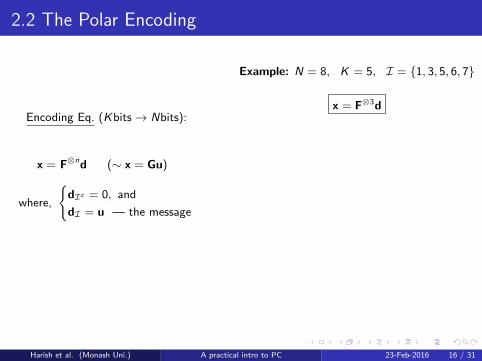
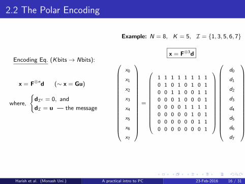
2.2 The Polar Encoding
Encoding Eq. (Kbits→ Nbits):
x = F⊗nd (∼ x = Gu)
where,
{dIc = 0, and
dI = u — the message
Example: N = 8, K = 5, I = {1, 3, 5, 6, 7}
x = F⊗3d
x0
x1
x2
x3
x4
x5
x6
x7
=
1 1 1 1 1 1 1 1
0 1 0 1 0 1 0 1
0 0 1 1 0 0 1 1
0 0 0 1 0 0 0 1
0 0 0 0 1 1 1 1
0 0 0 0 0 1 0 1
0 0 0 0 0 0 1 1
0 0 0 0 0 0 0 1
A very efficient O(N logN) implementation is available
Harish et al. (Monash Uni.) A practical intro to PC 23-Feb-2016 16 / 31
2.2 The Polar Encoding
Encoding Eq. (Kbits→ Nbits):
x = F⊗nd (∼ x = Gu)
where,
{dIc = 0, and
dI = u — the message
Example: N = 8, K = 5, I = {1, 3, 5, 6, 7}
x = F⊗3d
x0
x1
x2
x3
x4
x5
x6
x7
=
1 1 1 1 1 1 1 1
0 1 0 1 0 1 0 1
0 0 1 1 0 0 1 1
0 0 0 1 0 0 0 1
0 0 0 0 1 1 1 1
0 0 0 0 0 1 0 1
0 0 0 0 0 0 1 1
0 0 0 0 0 0 0 1
d0
d1
d2
d3
d4
d5
d6
d7
A very efficient O(N logN) implementation is available
Harish et al. (Monash Uni.) A practical intro to PC 23-Feb-2016 16 / 31

2.2 The Polar Encoding
Encoding Eq. (Kbits→ Nbits):
x = F⊗nd (∼ x = Gu)
where,
{dIc = 0, and
dI = u — the message
Example: N = 8, K = 5, I = {1, 3, 5, 6, 7}
x = F⊗3d
x0
x1
x2
x3
x4
x5
x6
x7
=
1 1 1 1 1 1 1 1
0 1 0 1 0 1 0 1
0 0 1 1 0 0 1 1
0 0 0 1 0 0 0 1
0 0 0 0 1 1 1 1
0 0 0 0 0 1 0 1
0 0 0 0 0 0 1 1
0 0 0 0 0 0 0 1
d0 = 0
d1
d2 = 0
d3
d4 = 0
d5
d6
d7
A very efficient O(N logN) implementation is available
Harish et al. (Monash Uni.) A practical intro to PC 23-Feb-2016 16 / 31
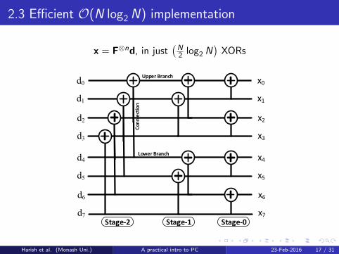
2.3 Efficient O(N log2 N) implementation
x = F⊗nd, in just(N2 log2 N
)XORs
x0
x1
x2
x3
x4
x5
x6
x7
d0
d1
d2
d3
d4
d5
d6
d7
Upper Branch
Con
n e
ctio
n
Stage-0Stage-1Stage-2
Lower Branch
Harish et al. (Monash Uni.) A practical intro to PC 23-Feb-2016 17 / 31
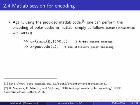
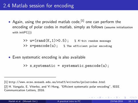
2.4 Matlab session for encoding
• Again, using the provided matlab code,[1] one can perform theencoding of polar codes in matlab, simply as follows (assume initialization
with initPC())
>> u=(rand(K,1)>0.5); % K-bit random message
>> x=pencode(u); % The efficient polar encoding
• Even systematic encoding is also available
>> x systematic = systematic pencode(u);
[1] http://www.ecse.monash.edu.au/staff/eviterbo/polarcodes.html
[2] H. Vangala, E. Viterbo, and Yi Hong, “Efficient systematic polar encoding”, IEEECommunication Letters, 2016.
Harish et al. (Monash Uni.) A practical intro to PC 23-Feb-2016 18 / 31
A Practical Introduction to Polar Codes(A very simple tutorial for beginners)
Harish Vangala, Yi Hong, and Emanuele Viterbo
Monash University, Australia
23 February, 2016
This presentation, and other useful resources such as MATLAB modules can be found here:
is.gd/polarcodes
(Or, http://www.ecse.monash.edu.au/staff/eviterbo/polarcodes.html)
Harish et al. (Monash Uni.) A practical intro to PC 23-Feb-2016 19 / 31

A Practical Introduction to Polar Codes
1 Code Construction
2 Encoding
3 Decoding
Harish et al. (Monash Uni.) A practical intro to PC 23-Feb-2016 20 / 31

A Practical Introduction to Polar Codes
1 Code Construction
2 Encoding
3 Decoding
Harish et al. (Monash Uni.) A practical intro to PC 23-Feb-2016 21 / 31
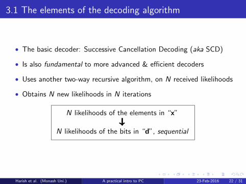
3.1 The elements of the decoding algorithm
• The basic decoder: Successive Cancellation Decoding (aka SCD)
• Is also fundamental to more advanced & efficient decoders
• Uses another two-way recursive algorithm, on N received likelihoods
• Obtains N new likelihoods in N iterations
N likelihoods of the elements in “x”
N likelihoods of the bits in “d”, sequential
Harish et al. (Monash Uni.) A practical intro to PC 23-Feb-2016 22 / 31

f (L1, L2)
g(L1, L2)
L1
L2
influences
• The two likelihood operations in use:L1
L2
−→f (L1, L2)
g(L1, L2)
=
L1L2+1L1+L2
L2 · L1 or L2/L1
• The second operation depends on the intermediate bit decisions from
the upper branch
Harish et al. (Monash Uni.) A practical intro to PC 23-Feb-2016 23 / 31

3.2 A numerical issue
• Numerical underflows are natural with using LRs
• Use of LLRs is suggested instead
• The new formulae become:l1
l2
−→ln f (e l1 , e l2)
ln g(e l1 , e l2)
=
ln(
1+exp(l1+l2)exp (l1)+exp (l2)
)l2 + l1 or l2 − l1
≈
sign(l1) sign(l2) min{|l1|, |l2|}
l2 + (−1)u l1
Harish et al. (Monash Uni.) A practical intro to PC 23-Feb-2016 24 / 31
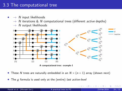
3.3 The computational tree
• → N input likelihoods→ N iterations & N computational trees (different active depths)→ N output likelihoods
3
7
2
6
1
5
0
4
6
7
4
5
2
3
0
1
(3) (2) (1) (0)
L(3)1
L(2)5
L(1)7
L(7)0
L(6)0
L(1)5
L(5)0
L(4)0
L(2)1
L(1)3
L(3)0
L(2)0
L(1)1
L(1)0
L(0)0
A computational-tree: example-1
fg
inactive
• These N trees are naturally embedded in an N × (n + 1) array (shown next)
• The g formula is used only at the (entire) last active-level
Harish et al. (Monash Uni.) A practical intro to PC 23-Feb-2016 25 / 31

3.3 The computational tree
• → N input likelihoods→ N iterations & N computational trees (different active depths)→ N output likelihoods
3
7
2
6
1
5
0
4
6
7
4
5
2
3
0
1
(3) (2) (1) (0)
L(3)2
L(2)6
L(1)6
L(0)7
L(0)6
L(1)4
L(0)5
L(0)4
L(2)2
L(1)2
L(0)3
L(0)2
L(1)0
L(0)1
L(0)0
A computational-tree: example-2
fg
inactive
• These N trees are naturally embedded in an N × (n + 1) array (shown next)
• The g formula is used only at the (entire) last active-level
Harish et al. (Monash Uni.) A practical intro to PC 23-Feb-2016 25 / 31
Bits LLRs
fg
inactivebit-availability
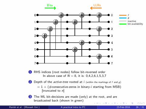
1 RHS indices (root nodes) follow bit-reversed orderIn above case of N = 8, it is: 0,4,2,6,1,5,3,7
2 Depth of the active-tree rooted at i (within the markings of f and g)
= 1 + (#consecutive-zeros in binary-i starting from MSB)[truncated to n]
3 The ML bit-decisions are made (only) at the root, and arebroadcasted back (shown in green)
Harish et al. (Monash Uni.) A practical intro to PC 23-Feb-2016 26 / 31
Bits LLRs
fg
inactivebit-availability
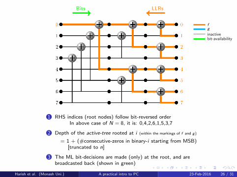
1 RHS indices (root nodes) follow bit-reversed orderIn above case of N = 8, it is: 0,4,2,6,1,5,3,7
2 Depth of the active-tree rooted at i (within the markings of f and g)
= 1 + (#consecutive-zeros in binary-i starting from MSB)[truncated to n]
3 The ML bit-decisions are made (only) at the root, and arebroadcasted back (shown in green)
Harish et al. (Monash Uni.) A practical intro to PC 23-Feb-2016 26 / 31

Bits LLRs
fg
inactivebit-availability
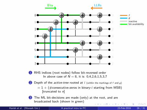
1 RHS indices (root nodes) follow bit-reversed orderIn above case of N = 8, it is: 0,4,2,6,1,5,3,7
2 Depth of the active-tree rooted at i (within the markings of f and g)
= 1 + (#consecutive-zeros in binary-i starting from MSB)[truncated to n]
3 The ML bit-decisions are made (only) at the root, and arebroadcasted back (shown in green)
Harish et al. (Monash Uni.) A practical intro to PC 23-Feb-2016 26 / 31

Bits LLRs
fg
inactivebit-availability
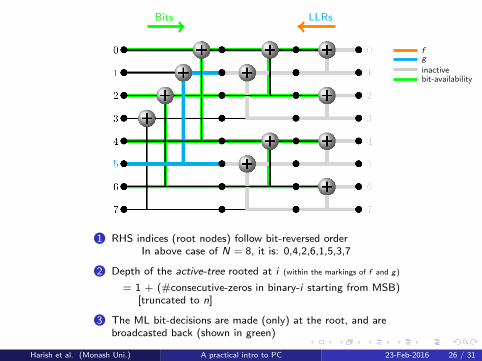
1 RHS indices (root nodes) follow bit-reversed orderIn above case of N = 8, it is: 0,4,2,6,1,5,3,7
2 Depth of the active-tree rooted at i (within the markings of f and g)
= 1 + (#consecutive-zeros in binary-i starting from MSB)[truncated to n]
3 The ML bit-decisions are made (only) at the root, and arebroadcasted back (shown in green)
Harish et al. (Monash Uni.) A practical intro to PC 23-Feb-2016 26 / 31
Bits LLRs
fg
inactivebit-availability
1 RHS indices (root nodes) follow bit-reversed orderIn above case of N = 8, it is: 0,4,2,6,1,5,3,7
2 Depth of the active-tree rooted at i (within the markings of f and g)
= 1 + (#consecutive-zeros in binary-i starting from MSB)[truncated to n]
3 The ML bit-decisions are made (only) at the root, and arebroadcasted back (shown in green)
Harish et al. (Monash Uni.) A practical intro to PC 23-Feb-2016 26 / 31

3.4 MATLAB session for decoding
Using the openly available matlab code[1]: (assume initialization with initPC())
>> u= (rand(K,1)>0.5); % Message
>> x= pencode(u); % Polar encoding
>> y= (2*x-1)*sqrt(Ec) + sqrt(N0/2)*randn(N,1); % AWGN
>> u decoded= pdecode(y);% The Successive Cancellation Decoding
>> logical(sum(u==u decoded)) % Check if properly decoded
ans =
1
[1] http://www.ecse.monash.edu.au/staff/eviterbo/polarcodes.html
Harish et al. (Monash Uni.) A practical intro to PC 23-Feb-2016 27 / 31
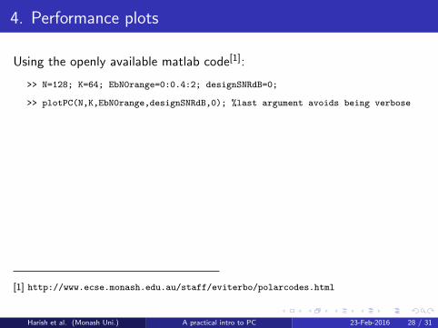
4. Performance plots
Using the openly available matlab code[1]:
>> N=128; K=64; EbN0range=0:0.4:2; designSNRdB=0;
>> plotPC(N,K,EbN0range,designSNRdB,0); %last argument avoids being verbose
Completed SNR points (out of 6):
0.00 dB (time taken:27.69 sec)
0.40 dB (time taken:27.18 sec)
0.80 dB (time taken:27.18 sec)
1.20 dB (time taken:27.16 sec)
1.60 dB (time taken:27.10 sec)
2.00 dB (time taken:40.55 sec)
Eb/N0 range (dB) : 0 0.4000 0.8000 1.2000 1.6000 2.0000
Frame Error Rates: 0.7080 0.5930 0.4790 0.3730 0.2400 0.1342
Bit Error Rates : 0.2311 0.1776 0.1393 0.1012 0.0646 0.0317
[1] http://www.ecse.monash.edu.au/staff/eviterbo/polarcodes.html
Harish et al. (Monash Uni.) A practical intro to PC 23-Feb-2016 28 / 31
0 0.5 1 1.5 2 2.5 3 3.5 4 4.510
−6
10−5
10−4
10−3
10−2
10−1
100
Eb/N0 in dB
Bit
Err
or
Ra
te (
BE
R)
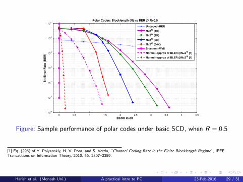
Polar Codes: Blocklength (N) vs BER @ R=0.5
Uncoded−BER
N=210
(1K)
N=211
(2K)
N=213
(8K)
N=216
(64K)
Shannon−Wall
Normal−approx of BLER @N=210
[1]
Normal−approx of BLER @N=216
[1]
Figure: Sample performance of polar codes under basic SCD, when R = 0.5
[1] Eq. (296) of Y. Polyanskiy, H. V. Poor, and S. Verdu, “Channel Coding Rate in the Finite Blocklength Regime”, IEEETransactions on Information Theory, 2010, 56, 2307–2359.
Harish et al. (Monash Uni.) A practical intro to PC 23-Feb-2016 29 / 31

1.5 2 2.5 3 3.5 4 4.5 5 5.5
10−6
10−5
10−4
10−3
10−2
10−1
100
Eb/N0 in dB
Bit
Err
or
Ra
te (
BE
R)
Polar Codes: Blocklength (N) vs BER @ R=0.9
Uncoded−BER
N=210
(1K)
N=211
(2K)
N=213
(8K)
N=216
(64K)
Shannon−Wall
Normal−approx of BLER @N=210
[1]
Normal−approx of BLER @N=216
[1]
Figure: Sample performance of polar codes under basic SCD, when R = 0.9
[1] Eq. (296) of Y. Polyanskiy, H. V. Poor, and S. Verdu, “Channel Coding Rate in the Finite Blocklength Regime”, IEEETransactions on Information Theory, 2010, 56, 2307–2359.
Harish et al. (Monash Uni.) A practical intro to PC 23-Feb-2016 30 / 31
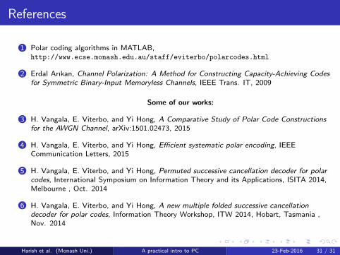
References
1 Polar coding algorithms in MATLAB,http://www.ecse.monash.edu.au/staff/eviterbo/polarcodes.html
2 Erdal Arıkan, Channel Polarization: A Method for Constructing Capacity-Achieving Codesfor Symmetric Binary-Input Memoryless Channels, IEEE Trans. IT, 2009
Some of our works:
3 H. Vangala, E. Viterbo, and Yi Hong, A Comparative Study of Polar Code Constructionsfor the AWGN Channel, arXiv:1501.02473, 2015
4 H. Vangala, E. Viterbo, and Yi Hong, Efficient systematic polar encoding, IEEECommunication Letters, 2015
5 H. Vangala, E. Viterbo, and Yi Hong, Permuted successive cancellation decoder for polarcodes, International Symposium on Information Theory and its Applications, ISITA 2014,Melbourne , Oct. 2014
6 H. Vangala, E. Viterbo, and Yi Hong, A new multiple folded successive cancellationdecoder for polar codes, Information Theory Workshop, ITW 2014, Hobart, Tasmania ,Nov. 2014
Harish et al. (Monash Uni.) A practical intro to PC 23-Feb-2016 31 / 31

![Construction and Performance of Polar Codes for ... · codes [3] in 1949, Hamming codes [4] in 1950, Convolutional codes [5] in 1955, Reed-Solomon codes [6] in 1960, Low-Density Parity-Check](https://img.pdfslide.us/doc/110x75/606e21e8d7719369556b73e0/construction-and-performance-of-polar-codes-for-codes-3-in-1949-hamming-codes.jpg)