Embed Size (px)
Citation preview

1
Polar Codes for Broadcast Channels
Naveen Goela†, Emmanuel Abbe♯, and Michael Gastpar†
Abstract
Polar codes are introduced for discrete memoryless broadcast channels. For m-user deterministic
broadcast channels, polarization is applied to map uniformly random message bits from m independent
messages to one codeword while satisfying broadcast constraints. The polarization-based codes achieve
rates on the boundary of the private-message capacity region. For two-user noisy broadcast channels,
polar implementations are presented for two information-theoretic schemes: i) Cover’s superposition
codes; ii) Marton’s codes. Due to the structure of polarization, constraints on the auxiliary and channel-
input distributions are identified to ensure proper alignment of polarization indices in the multi-user
setting. The codes achieve rates on the capacity boundary of a few classes of broadcast channels (e.g.,
binary-input stochastically degraded). The complexity of encoding and decoding is O(n log n) where n
is the block length. In addition, polar code sequences obtain a stretched-exponential decay of O(2−nβ
)
of the average block error probability where 0 < β < 12 . Reproducible experiments for finite block
lengths n = 512, 1024, 2048 corroborate the theory.∗
Index Terms
Polar Codes, Deterministic Broadcast Channel, Cover’s Superposition Codes, Marton’s Codes.
I. INTRODUCTION
This work was presented in part at the International Zurich Seminar on Communications, Zurich, Switzerland on March 1,
2012, and the IEEE International Symposium on Information Theory, Istanbul, Turkey on July 9, 2013.
∗ Further reproducible experiments to supplement the theory are in progress.
†N. Goela and M. C. Gastpar are with the Department of Electrical Engineering and Computer Science, University of
California, Berkeley, Berkeley, CA 94720-1770 USA (e-mail: ngoela, [email protected]) and also with the School of
Computer and Communication Sciences, Ecole Polytechnique Federale (EPFL), Lausanne, Switzerland (e-mail: naveen.goela,
♯E. Abbe is currently with the School of Engineering and Applied Sciences, Princeton University, Princeton, NJ, 08544 USA
(e-mail: [email protected]).

2
INTRODUCED by T. M. Cover in 1972, the broadcast problem consists of a single source transmitting
m independent private messages to m receivers through a single discrete, memoryless, broadcast chan-
nel (DM-BC) [1]. The private-message capacity region is known if the channel structure is deterministic,
degraded, less-noisy, or more-capable [2]. For general classes of DM-BCs, there exist inner bounds such
as Marton’s inner bound [3] and outer bounds such as the Nair-El-Gamal outer bound [4]. One difficult
aspect of the broadcast problem is to design an encoder which maps m independent messages to a single
codeword of symbols which are transmitted simultaneously to all receivers. Several codes relying on
random binning, superposition, and Marton’s strategy have been analyzed in the literature (see e.g., the
overview in [5]).
A. Overview of Contributions
The present paper focuses on low-complexity codes for broadcast channels based on polarization
methods. Polar codes were invented originally by Arıkan and were shown to achieve the capacity of
binary-input, symmetric, point-to-point channels with O(n log n) encoding and decoding complexity
where n is the code length [6]. In this paper, we obtain the following results.
• Polar codes for deterministic, linear and non-linear, binary-output, m-user DM-BCs (cf. [7]). The
capacity-achieving broadcast codes implement low-complexity random binning, and are related to
polar codes for other multi-user scenarios such as Slepian-Wolf distributed source coding [8], [9],
and multiple-access channel (MAC) coding [10]. For deterministic DM-BCs, the polar transform is
applied to channel output variables. Polarization is useful for shaping uniformly random message
bits from m independent messages into non-equiprobable codeword symbols in the presence of hard
broadcast constraints. As discussed in Section I-B1 and referenced in [11]–[13], it is difficult to design
low-complexity parity-check (LDPC) codes or belief propagation algorithms for the deterministic
DM-BC due to multi-user broadcast constraints.
• Polar codes for general two-user DM-BCs based on Cover’s superposition coding strategy. In the
multi-user setting, constraints on the auxiliary and channel-input distributions are placed to ensure
alignment of polarization indices. The achievable rates lie on the boundary of the capacity region
for certain classes of DM-BCs such as binary-input stochastically degraded channels.
• Polar codes for general two-user DM-BCs based on Marton’s coding strategy. In the multi-user set-
ting, due to the structure of polarization, constraints on the auxiliary and channel-input distributions
are identified to ensure alignment of polarization indices. The achievable rates lie on the boundary of
the capacity region for certain classes of DM-BCs such as binary-input semi-deterministic channels.

3
• For the above broadcast polar codes, the asymptotic decay of the average error probability under
successive cancelation decoding at the broadcast receivers is established to be O(2−nβ
) where 0 <
β < 12 . The error probability is analyzed by averaging over polar code ensembles. In addition,
properties such as the chain rule of the Kullback-Leibler divergence between discrete probability
measures are exploited.
• Reproducible experiments are provided for finite block lengths n = 512, 1024, 2048. The results of
the experiments corroborate the theory.
Throughout the paper, for different broadcast coding strategies, a systems-level block diagram of the
communication channel and polar transforms is provided.
B. Relation to Prior Work
1) Deterministic Broadcast Channels: The deterministic broadcast channel has received considerable
attention in the literature (e.g. due to related extensions such as secure broadcast, broadcasting with side
information, and index coding [14], [15]). Several practical codes have been designed. For example, the
authors of [11] propose sparse linear coset codes to emulate random binning and survey propagation
to enforce broadcast channel constraints. In [12], the authors propose enumerative source coding and
Luby-Transform codes for deterministic DM-BCs specialized to interference-management scenarios. Ad-
ditional research includes reinforced belief propagation with non-linear coding [13]. To our knowledge,
polarization-based codes provide provable guarantees for achieving rates on the capacity-boundary in the
general case.
2) Polar Codes for Multi-User Settings: Subsequent to the derivation of channel polarization in [6]
and the refined rate of polarization in [16], polarization methods have been extended to analyze multi-
user information theory problems. In [10], a joint polarization method is proposed for m-user MACs
with connections to matroid theory. Polar codes were extended for several other multi-user settings:
arbitrarily-permuted parallel channels [17], degraded relay channels [18], cooperative relaying [19], and
wiretap channels [20]–[22]. In addition, several binary multi-user communication scenarios including
the Gelfand-Pinsker problem, and Wyner-Ziv problem were analyzed in [23, Chapter 4]. Polar codes
for lossless and lossy source compression were investigated respectively in [8] and [24]. In [8], source
polarization was extended to the Slepian-Wolf problem involving distributed sources. The approach is
based on an “onion-peeling” encoding of sources, whereas a joint encoding is proposed in [25]. In [9],
a unified approach is provided for the Slepian-Wolf problem based on generalized monotone chain rules
of entropy. To our knowledge, the design of polarization-based broadcast codes is relatively new.

4
0
1
2
0
1
0
1
X
Y1
Y2
b
b
b
b
b
b
b
0 0.2 0.4 0.6 0.8 1 1.2 1.4 1.60
0.2
0.4
0.6
0.8
1
1.2
1.4
1.6
Capacity Region of Blackwell Channel
R1
R2
Fig. 1. Blackwell Channel: An example of a deterministic broadcast channel with m = 2 broadcast users. The channel is
defined as Y1 = f1(X) and Y2 = f2(X) where the non-linear functions f1(x) = max(x− 1, 0) and f2(x) = min(x, 1). The
private-message capacity region of the Blackwell channel is drawn. For different input distributions PX(x), the achievable rate
points are contained within corresponding polyhedrons in Rm+ .
3) Binary vs. q-ary Polarization: The broadcast codes constructed in the present paper for DM-BCs
are based on polarization for binary random variables. However, in extending to arbitrary alphabet sizes,
a large body of prior work exists and has focused on generalized constructions and kernels [26], and
generalized polarization for q-ary random variables and q-ary channels [27]–[30]. The reader is also
referred to the monograph in [31] containing a clear overview of polarization methods.
C. Notation
An index set 1, 2, . . . ,m is abbreviated as [m]. An m × n matrix array of random variables is
comprised of variables Yi(j) where i ∈ [m] represents the row and j ∈ [n] the column. The notation
Y k:ℓi , Yi(k), Yi(k + 1), . . . , Yi(ℓ) for k ≤ ℓ. When clear by context, the term Y n
i represents Y 1:ni .
In addition, the notation for the random variable Yi(j) is used interchangeably with Y ji . The notation
f(n) = O(g(n)) means that there exists a constant κ such that f(n) ≤ κg(n) for sufficiently large
n. For a set S , clo(S) represents set closure, and co(S) the convex hull operation over set S . Let
hb(x) = −x log2(x)−(1−x) log2(1−x) denote the binary entropy function. Let a∗b , (1−a)b+a(1−b).
II. MODEL
Definition 1 (Discrete, Memoryless Broadcast Channel): The discrete memoryless broadcast channel
(DM-BC) with m broadcast receivers consists of a discrete input alphabet X , discrete output alphabets
Yi for i ∈ [m], and a conditional distribution PY1,Y2,...,Ym|X(y1, y2, . . . , ym|x) where x ∈ X and yi ∈ Yi.

5
Definition 2 (Private Messages): For a DM-BC with m broadcast receivers, there exist m private
messages Wii∈[m] such that each message Wi is composed of nRi bits and (W1,W2, . . . ,Wm) is
uniformly distributed over [2nR1 ]× [2nR2 ]× · · · × [2nRm ].
Definition 3 (Channel Encoding and Decoding): For the DM-BC with independent messages, let the
vector of rates ~R ,
[
R1 R2 . . . Rm
]T. An (~R, n) code for the DM-BC consists of one encoder
xn : [2nR1 ]× [2nR2 ]× · · · × [2nRm ] → X n,
and m decoders specified by Wi : Yni → [2nRi ] for i ∈ [m]. Based on received observations Yi(j)j∈[n],
each decoder outputs a decoded message Wi.
Definition 4 (Average Probability of Error): The average probability of error P(n)e for a DM-BC code
is defined to be the probability that the decoded message at all receivers is not equal to the transmitted
message,
P (n)e = P
m∨
i=1
Wi
(
Yi(j)j∈[n])
6=Wi
.
Definition 5 (Private-Message Capacity Region): If there exists a sequence of (~R, n) codes with P(n)e →
0, then the rates ~R ∈ Rm+ are achievable. The private-message capacity region is the closure of the set
of achievable rates.
III. DETERMINISTIC BROADCAST CHANNELS
Definition 6 (Deterministic DM-BC): Define m deterministic functions fi(x) : X → Yi for i ∈ [m].
The deterministic DM-BC with m receivers is defined by the following conditional distribution
PY1,Y2,...,Ym|X(y1, y2, . . . , ym|x) =m∏
i=1
1[yi=fi(x)]. (1)
A. Capacity Region
Proposition 1 (Marton [32], Pinsker [33]): The capacity region of the deterministic DM-BC includes
those rate-tuples ~R ∈ Rm+ in the region
CDET−BC , co(
clo(
⋃
X,Yii∈[m]
R(
X, Yii∈[m]
)
))
, (2)
where the polyhedral region R(X, Yii∈[m]) is given by
R ,
~R∣
∣
∣
∑
i∈S
Ri < H(Yii∈S), ∀S ⊆ [m]
. (3)

6
The union in Eqn. (2) is over all random variables X,Y1, Y2, . . . , Ym with joint distribution induced by
PX(x) and Yi = fi(X).
Example 1 (Blackwell Channel): In Figure 1, the Blackwell channel is depicted with X = 0, 1, 2
and Yi = 0, 1. For any fixed distribution PX(x), it is seen that PY1Y2(y1, y2) has zero mass for the
pair (1, 0). Let α ∈ [12 ,23 ]. Due to the symmetry of this channel, the capacity region is the union of two
regions,
(R1, R2) : R1 ≤ hb(α), R2 ≤ hb(α
2), R1 +R2 ≤ hb(α) + α,
(R1, R2) : R1 ≤ hb(α
2), R2 ≤ hb(α), R1 +R2 ≤ hb(α) + α,
where the first region is achieved with input distribution PX(0) = PX(1) =α2 , and the second region is
achieved with PX(1) = PX(2) =α2 [2, Lec. 9]. The sum rate is maximized for a uniform input distribution
which yields a pentagonal achievable rate region: R1 ≤ hb(13 ), R2 ≤ hb(
13 ), R1 +R2 ≤ log2 3. Figure 1
illustrates the capacity region.
B. Main Result
Theorem 1 (Polar Code for Deterministic DM-BC): Consider an m-user deterministic DM-BC with
arbitrary discrete input alphabet X , and binary output alphabets Yi ∈ 0, 1. Fix input distribution
PX(x) where x ∈ X and constant 0 < β < 12 . Let π : [m] → [m] be a permutation on the index set of
receivers. Let the vector
~R ,
[
Rπ(1) Rπ(2) . . . Rπ(m)
]T.
There exists a sequence of polar broadcast codes over n channel uses which achieves rates ~R where the
rate for receiver π(i) ∈ [m] is bounded as
0 ≤ Rπ(i) < H(
Yπ(i)|Yπ(k)k=1:i−1
)
.
The average error probability of this code sequence decays as P(n)e = O(2−n
β
). The complexity of
encoding and decoding is O(n log n).
Remark 1: To prove the existence of low-complexity broadcast codes, a successive randomized protocol
is introduced in Section V-A which utilizes o(n) bits of randomness at the encoder. A deterministic
encoding protocol is also presented.
Remark 2: The achievable rates for a fixed input distribution PX(x) are the vertex points of the
polyhedral rate region defined in (3). To achieve non-vertex points, the following coding strategies could

7
0 0.2 0.4 0.6 0.8 1 1.2 1.4 1.60
0.2
0.4
0.6
0.8
1
1.2
1.4
1.6
Blackwell Channel, Polar Code n = 2048
R1
R2
P(n)e = 0.0006
P(n)e = 0.0024
P(n)e = 0.0095
P(n)e = 0.0953
P(n)e = 1
P(n)e = 0.6351
Fig. 2. Polar Code for Blackwell Channel: Broadcast code approaching the capacity boundary point of (R1, R2) = (hb(23), 2
3).
be applied: time-sharing; rate-splitting for the deterministic DM-BC [34]; polarization by Arıkan utilizing
generalized chain rules of entropy [9]. For certain input distributions PX(x), as illustrated in Figure 1
for the Blackwell channel, a subset of the achievable vertex points lie on the capacity boundary.
Remark 3: Polarization of channels and sources extends to q-ary alphabets (see e.g. [27]). Similarly,
it is entirely possible to extend Theorem 1 to include DM-BCs with q-ary output alphabets.
C. Experimental Results For The Blackwell Channel
As an experiment for the Blackwell channel described in Example 1, the target rate pair on the capacity
boundary is selected to be (R1, R2) = (hb(23),
23). Note that R1 + R2 = log2 3 which is the maximum
sum rate possible for any input distribution. To achieve the target rate pair, the input distribution PX(x)

8
TABLE I
P(n)e FOR DIFFERENT RATE PAIRS ACHIEVED FOR THE BLACKWELL CHANNEL
n n n n
(R1, R2) 512 1024 2048 4096
(0.73, 0.53) 0.106 0.0518 0.0195 0.0051
(0.76, 0.55) 0.201 0.1356 0.0631 0.0194
(0.79, 0.57) 0.3799 0.3177 0.2246 0.1188
(0.82, 0.59) 0.5657 0.5606 0.5079 0.4070
(0.85, 0.61) 0.7849 0.8181 0.8286 0.8133
(0.87, 0.63) 0.9454 0.9757 0.9866 0.9936
(0.90, 0.65) 0.9986 1.0000 1.0000 1.0000
is uniform. The output distribution is then PY1Y2(0, 0) = PY1Y2
(0, 1) = PY1Y2(1, 1) = 1
3 . For the output
distribution, H(Y1) = hb(23) and H(Y2|Y1) =
23 . According to Theorem 1, these distributions permit polar
codes approaching the target boundary rate pair. Figure 2 shows the average probability of error P(n)e for
block length n = 2048 with selected rate pairs approaching the capacity boundary. The broadcast code
employs a deterministic rule as opposed to a randomized rule at the encoder as described in Section V-A.
Table I provides results of experiments for different block lengths for a randomized rule at the encoder.
While the randomized rule is important for the proof, the deterministic rule provides better error results
in practice. All data points for error probabilities were generated using 104 codeword transmissions.
Remark 4 (Zero Error vs. Average Error): A zero-error coding scheme is trivial for rate pairs (R1, R2)
within the triangle: (0, 0), (0, 1), (1, 0). Beyond the triangular region, it is possible to achieve zero-error
throughout the whole capacity region by purging the polar code-book of any codewords causing error at
the encoder. However, unless there exists an efficient method to enumerate the code-book, the purging
process is not feasible with low-complexity since there exist an exponential number of codewords.
IV. OVERVIEW OF POLARIZATION METHOD
FOR DETERMINISTIC DM-BCS
For the proof of Theorem 1, we utilize binary polarization theorems. By contrast to polarization for
point-to-point channels, in the case of deterministic DM-BCs, the polar transform is applied to the output
random variables of the channel.

9
A. Polar Transform
Consider an input distribution PX(x) to the deterministic DM-BC. Over n channel uses, the input
random variables to the channel are given by
X1:n = X1,X2, . . . ,Xn,
where Xj ∼ PX are independent and identically distributed (i.i.d.) random variables. The channel output
variables are given by Yi(j) = fi(X(j)) where fi(·) are the deterministic functions to each broadcast
receiver. Denote the random matrix of channel output variables by
Y ,
Y 11 Y 2
1 Y 31 . . . Y n1
Y 12 Y 2
2 Y 32 . . . Y n2
......
... . . ....
Y 1m Y 2
m Y 3m . . . Y nm
, (4)
where Y ∈ Fm×n2 . For n = 2ℓ and ℓ ≥ 1, the polar transform is defined as the following invertible linear
transformation,
U = YGn (5)
where Gn ,
1 0
1 1
⊗log2 n
Bn.
The matrix Gn ∈ Fn×n2 is formed by multiplying a matrix of successive Kronecker matrix-products
(denoted by⊗
) with a bit-reversal matrix Bn introduced by Arıkan [8]. The polarized random matrix
U ∈ Fm×n2 is indexed as
U ,
U11 U2
1 U31 . . . Un1
U12 U2
2 U32 . . . Un2
......
... . . ....
U1m U2
m U3m . . . Unm
. (6)
B. Joint Distribution of Polarized Variables
Consider the channel output distribution PY1Y2···Ymof the deterministic DM-BC induced by input
distribution PX(x). The j-th column of the random matrix Y is distributed as (Y j1 , Y
j2 , · · ·, Y
jm) ∼

10
PY1Y2···Ym. Due to the memoryless property of the channel, the joint distribution of all output variables
is
PY n1 Y
n2 ···Y n
m
(
yn1 , yn2 , · · ·, y
nm
)
=
n∏
j=1
PY1Y2···Ym
(
yj1, yj2, . . . , y
jm
)
. (7)
The joint distribution of the matrix variables in Y is characterized easily due to the i.i.d. structure.
The polarized random matrix U does not have an i.i.d. structure. However, one way to define the joint
distribution of the variables in U is via the polar transform equation (5). An alternate representation is
via a decomposition into conditional distributions as follows1.
PUn1 U
n2 ···Un
m
(
un1 , un2 , · · ·u
nm
)
=
m∏
i=1
n∏
j=1
P(
ui(j)∣
∣
∣u1:j−1i , u1:nk k∈[1:i−1]
)
. (8)
As derived by Arıkan in [8] and summarized in Section IV-E, the conditional probabilities in (8) and
associated likelihoods may be computed using a dynamic programming method which “divides-and-
conquers” the computations efficiently.
C. Polarization of Conditional Entropies
Proposition 2 (Polarization [8]): Consider the pair of random matrices (Y,U) related through the
polar transformation in (5). For i ∈ [m] and any ǫ ∈ (0, 1), define the set of indices
A(n)i ,
j ∈ [n] : H(
Ui(j)∣
∣
∣U1:j−1i , Y 1:n
k k∈[1:i−1]
)
≥ 1− ǫ
. (9)
Then in the limit as n→ ∞,
1
n
∣
∣
∣A
(n)i
∣
∣
∣→ H(Yi|Y1Y2 · · · Yi−1). (10)
For sufficiently large n, Theorem 2 establishes that there exist approximately nH (Yi|Y1Y2 · · · Yi−1)
indices per row i ∈ [m] of random matrix U for which the conditional entropy is close to 1. The
total number of indices in U for which the conditional entropy terms polarize to 1 is approximately
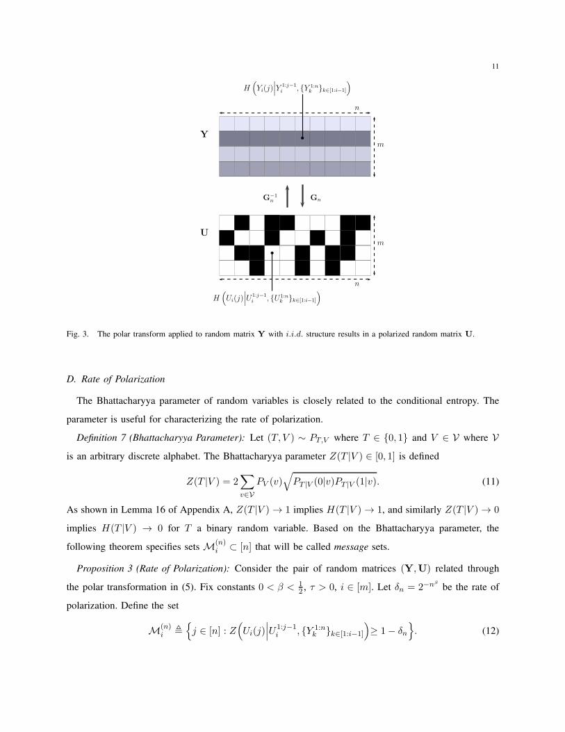
nH(Y1Y2 · · · Ym). The polarization phenomenon is illustrated in Figure 3.
Remark 5: Since the polar transform Gn is invertible, U1:nk k∈[1:i−1] are in one-to-one correspondence
with Y 1:nk k∈[1:i−1]. Therefore the conditional entropies H
(
Ui(j)∣
∣U1:j−1i , U1:n
k k∈[1:i−1]
)
also polarize
to 0 or 1.
1The abbreviated notation of the form P (a|b) which appears in (8) indicates PA|B(a|b), i.e. the conditional probability
PA = a|B = b where A and B are random variables.
11
GnG−1n
H(
Yi(j)∣
∣
∣Y
1:j−1i , Y 1:n
k k∈[1:i−1]
)
H(
Ui(j)∣
∣
∣U
1:j−1i , U1:n
k k∈[1:i−1]
)
Y
U
m
m
n
n
Fig. 3. The polar transform applied to random matrix Y with i.i.d. structure results in a polarized random matrix U.
D. Rate of Polarization
The Bhattacharyya parameter of random variables is closely related to the conditional entropy. The
parameter is useful for characterizing the rate of polarization.
Definition 7 (Bhattacharyya Parameter): Let (T, V ) ∼ PT,V where T ∈ 0, 1 and V ∈ V where V
is an arbitrary discrete alphabet. The Bhattacharyya parameter Z(T |V ) ∈ [0, 1] is defined
Z(T |V ) = 2∑
v∈V
PV (v)√
PT |V (0|v)PT |V (1|v). (11)
As shown in Lemma 16 of Appendix A, Z(T |V ) → 1 implies H(T |V ) → 1, and similarly Z(T |V ) → 0
implies H(T |V ) → 0 for T a binary random variable. Based on the Bhattacharyya parameter, the
following theorem specifies sets M(n)i ⊂ [n] that will be called message sets.
Proposition 3 (Rate of Polarization): Consider the pair of random matrices (Y,U) related through
the polar transformation in (5). Fix constants 0 < β < 12 , τ > 0, i ∈ [m]. Let δn = 2−n
β
be the rate of
polarization. Define the set
M(n)i ,
j ∈ [n] : Z(
Ui(j)∣
∣
∣U1:j−1i , Y 1:n
k k∈[1:i−1]
)
≥ 1− δn
. (12)

12
Then there exists an No = No(β, τ) such that
1
n
∣
∣
∣M
(n)i
∣
∣
∣≥ H(Yi|Y1Y2 · · · Yi−1)− τ, (13)
for all n > No.
The proposition is established via the Martingale Convergence Theorem by defining a super-martingale
with respect to the Bhattacharyya parameters [6] [8]. The rate of polarization is characterized by Arıkan
and Telatar in [16].
Remark 6: The message sets M(n)i are computed “offline” only once during a code construction phase.
The sets do not depend on the realization of random variables. In the following Section IV-E, a Monte
Carlo sampling approach for estimating Bhattacharyya parameters is reviewed. Other highly efficient
algorithms are known in the literature for finding the message indices (see e.g. Tal and Vardy [35]).
E. Estimating Bhattacharyya Parameters
As shown in Lemma 11 in Appendix A, one way to estimate the Bhattacharyya parameter Z(T |V ) is
to sample from the distribution PT,V (t, v) and evaluate ET,V
√
ϕ(T, V ). The function ϕ(t, v) is defined
based on likelihood ratios
L(v) ,PT |V (0|v)
PT |V (1|v),
L−1(v) ,PT |V (1|v)
PT |V (0|v).
Similarly, to determine the indices in the message sets M(n)i defined in Proposition 3, the Bhat-
tacharyya parameters Z(
Ui(j)∣
∣
∣U1:j−1i , Y 1:n
k k∈[i−1]
)
must be estimated efficiently. For n ≥ 2, define
the likelihood ratio
L(i,j)n
(
u1:j−1i , y1:nk k∈[1:i−1]
)
,P
(
Ui(j) = 0∣
∣
∣U1:j−1i = u1:j−1
i , Y 1:nk = y1:nk k∈[1:i−1]
)
P
(
Ui(j) = 1∣
∣
∣U1:j−1i = u1:j−1
i , Y 1:nk = y1:nk k∈[1:i−1]
) . (14)
The dynamic programming method given in [8] allows for a recursive computation of the likelihood ratio.
Define the following sub-problems
Ξ1 = L(i,j)n
2
(
u1:2j−2i,o ⊕ u1:2j−2
i,e , y1:n
2
k k∈[1:i−1]
)
,
Ξ2 = L(i,j)n
2
(
u1:2j−2i,e , y
n
2+1:n
k k∈[1:i−1]
)
,

13
0 0.1 0.2 0.3 0.4 0.5 0.6 0.7 0.8 0.9 10
0.1
0.2
0.3
0.4
0.5
0.6
0.7
0.8
0.9
1
Indices j ∈ [n] Normalized By Block Length n
Sorted
EntropiesH(U
1(j)|U
1:j−1
1)
Polarization Curves n = 512, 1024, 2048
0 0.1 0.2 0.3 0.4 0.5 0.6 0.7 0.8 0.9 10
0.1
0.2
0.3
0.4
0.5
0.6
0.7
0.8
0.9
1
Polarization Curves n = 512, 1024, 2048
Indices j ∈ [n] Normalized By Block Length n
Sorted
EntropiesH(U
2(j)|U
1:j−1
2,Y
1:n
1)
Fig. 4. Polarization Curves: (a) Bernoulli source polarization; (b) Polarization of conditional entropies.
where the notation u1:2j−2i,o and u1:2j−2
i,e represents the odd and even indices respectively of the sequence
u1:2j−2i . The recursive computation of the likelihoods is characterized by
L(i,2j−1)n
(
u1:2j−2i , y1:nk k∈[1:i−1]
)
=Ξ1Ξ2 + 1
Ξ1 + Ξ2.
L(i,2j)n
(
u1:2j−1i , y1:nk k∈[1:i−1]
)
= (Ξ1)γ Ξ2,
where γ = 1 if ui(2j − 1) = 0 and γ = −1 if ui(2j − 1) = 1. In the above recursive computations, the
base case is for sequences of length n = 2.
The dynamic programming technique may be modified to estimate target probabilities, Bhattacharyya
parameters, and also conditional entropies directly. Figure 4 shows the results of polarizing a joint
distribution PY1Y2(y1, y2) when PY1Y2
(0, 0) = PY1Y2(0, 1) = PY1Y2
(1, 1) = 13 . In the plot to the left, a
single-source polarization result is shown for an i.i.d. Bernoulli source PY1(0) = 2
3 . In the plot to the right,
a conditional polarization result is given for PY1Y2(y1, y2). The block lengths are n = 512, 1024, 2048.
V. PROOF OF THEOREM 1
The proof of Theorem 1 is based on binary polarization theorems as discussed in Section IV. The
random coding arguments of C. E. Shannon prove the existence of capacity-achieving codes for point-to-
point channels. Furthermore, random binning and joint-typicality arguments suffice to prove the existence
of capacity-achieving codes for the deterministic DM-BC. However, it is shown in this section that there
exist capacity-achieving polar codes for the binary-output deterministic DM-BC.

14
A. Broadcast Code Based on Polarization
The ordering of the receivers’ rates in ~R is arbitrary due to symmetry. Therefore, let π(i) = i be the
identity permutation which denotes the successive order in which the message bits are allocated for each
receiver. The encoder must map m independent messages (W1,W2, . . . ,Wm) uniformly distributed over
[2nR1 ] × [2nR2 ] × · · · × [2nRm ] to a codeword xn ∈ X n. To construct a codeword for broadcasting m
independent messages, the following binary sequences are formed at the encoder: u1:n1 , u1:n2 , . . . , u1:nm .
To determine a particular bit ui(j) in the binary sequence u1:ni , if j ∈ M(n)i , the bit is selected as a
uniformly distributed message bit intended for receiver i ∈ [m]. As defined in (12) of Proposition 3, the
message set M(n)i represents those indices for bits transmitted to receiver i. The remaining non-message
indices in the binary sequence u1:ni for each user i ∈ [m] are computed either according to a deterministic
or random mapping.
1) Deterministic Mapping: Consider a class of deterministic boolean functions indexed by i ∈ [m]
and j ∈ [n]:
ψ(i,j) : 0, 1n(max0,i−1)+j−1 → 0, 1. (15)
As an example, consider the deterministic boolean function based on the maximum a posteriori polar
coding rule.
ψ(i,j)MAP
(
u1:j−1i , y1:nk k∈[1:i−1]
)
, argmaxu∈0,1
P
(
Ui(j) = u∣
∣
∣U1:j−1i = u1:j−1
i , Y 1:nk = y1:nk k∈[1:i−1]
)
.
(16)
2) Random Mapping: Consider a class of random boolean functions indexed by i ∈ [m] and j ∈ [n]:
Ψ(i,j) : 0, 1n(max0,i−1)+j−1 → 0, 1. (17)
As an example, consider the random boolean function
Ψ(i,j)RAND
(
u1:j−1i , y1:nk k∈[1:i−1]
)
,
0, w.p. λ0
(
u1:j−1i , y1:nk k∈[1:i−1]
)
,
1, w.p. 1− λ0
(
u1:j−1i , y1:nk k∈[1:i−1]
)
,
(18)
where
λ0
(
u1:j−1i , y1:nk k∈[1:i−1]
)
, P
(
Ui(j) = 0∣
∣
∣U1:j−1i = u1:j−1
i , Y 1:nk = y1:nk k∈[1:i−1]
)
.
The random boolean function Ψ(i,j)RAND may be thought of as a vector of Bernoulli random variables
indexed by the input to the function. Each Bernoulli random variable of the vector has a fixed probability
of being one or zero that is well-defined.

15
3) Mapping From Messages To Codeword: The binary sequences u1:ni for i ∈ [m] are formed
successively bit by bit. If j ∈ M(n)i , then the bit ui(j) is one message bit from the uniformly distributed
message Wi intended for user i. If j /∈ M(n)i , ui(j) = ψ
(i,j)MAP
(
u1:j−1i , y1:nk k∈[1:i−1]
)
in the case of a
deterministic mapping, or ui(j) = Ψ(i,j)RAND
(
u1:j−1i , y1:nk k∈[1:i−1]
)
in the case of a random mapping.
The encoder then applies the inverse polar transform for each sequence: y1:ni = u1:ni G−1n . The codeword
xn is formed symbol-by-symbol as follows:
x(j) ∈m⋂
i=1
f−1i (yi(j)) .
If the intersection set is empty, the encoder declares a block error. A block error only occurs at the
encoder.
4) Decoding at Receivers: If the encoder succeeds in transmitting a codeword xn, each receiver
obtains the sequence y1:ni noiselessly and applies the polar transform Gn to recover u1:ni exactly. Since
the message indices M(n)i are known to each receiver, the message bits in u1:ni are decoded correctly by
receiver i.
B. Total Variation Bound
While the deterministic mapping ψ(i,j)MAP performs well in practice, the average probability of error P
(n)e
of the coding scheme is more difficult to analyze in theory. The random mapping Ψ(i,j)RAND at the encoder
is more amenable to analysis via the probabilistic method. Towards that goal, consider the following
probability measure defined on the space of tuples of binary sequences2.
Q(
un1 , un2 , · · ·, u
nm
)
,
m∏
i=1
n∏
j=1
Q(
ui(j)∣
∣
∣u1:j−1i , u1:nk k∈[1:i−1]
)
. (19)
where the conditional probability measure
Q(
ui(j)∣
∣
∣u1:j−1i , u1:nk k∈[1:i−1]
)
,
12 , if j ∈ M
(n)i ,
P(
ui(j)∣
∣
∣u1:j−1i , u1:nk k∈[1:i−1]
)
, otherwise.
The probability measure Q defined in (19) is a perturbation of the joint probability measure P defined
in (8) for the random variables Ui(j). The only difference in definition between P and Q is due to those
indices in message set M(n)i . The following lemma provides a bound on the total variation distance
between P and Q.
2A related proof technique was provided for lossy source coding based on polarization in a different context [24]. In the
present paper, a different proof is supplied that utilizes the chain rule for KL-divergence.

16
Lemma 1: (Total Variation Bound) Let probability measures P and Q be defined as in (8) and (19)
respectively. Let 0 < β < 1. For sufficiently large n, the total variation distance between P and Q is
bounded as
∑
u1:nk k∈[m]
∣
∣
∣P(
u1:nk k∈[m]
)
−Q(
u1:nk k∈[m]
)
∣
∣
∣≤ 2−n
β
.
Proof: See Section B of the Appendices.
C. Analysis of the Average Probability of Error
For the m-user deterministic DM-BC, an error event occurs at the encoder if a codeword xn is unable
to be constructed symbol by symbol according to the broadcast protocol described in Section V-A. Define
the following set consisting of m-tuples of binary sequences,
T ,
(yn1 , yn2 , . . . , y
nm) : ∃j ∈ [n],
m⋂
i=1
f−1i (yi(j)) = ∅
. (20)
The set T consists of those m-tuples of binary output sequences which are inconsistent due to the
properties of the deterministic channel. In addition, due to the one-to-one correspondence between
sequences u1:ni and y1:ni , denote by T the set of m-tuples (un1 , un2 , . . . , u
nm) that are inconsistent.
For the broadcast protocol, the rate Ri =1n
∣
∣M(n)i
∣
∣ for each receiver. Let the total sum rate for all
broadcast receivers be RΣ =∑
i∈[m]Ri. If the encoder uses a fixed deterministic map ψ(i,j) in the
broadcast protocol, the average probability of error is
P (n)e
[
ψ(i,j)]
=1
2nRΣ
∑
u1:nk k∈[m]
[1[(un1 ,u
n2 ,...,u
nm)∈T ]
·∏
i∈[m]
j∈[n]:j /∈M(n)i
1[ψ(i,j)(u1:j−1i ,y1:nk k∈[1:i−1])=ui(j)]
]
. (21)
In addition, if the random maps Ψ(i,j) are used at the encoder, the average probability of error is a random
quantity given by
P (n)e
[
Ψ(i,j)]
=1
2nRΣ
∑
u1:nk k∈[m]
[1[(un1 ,u
n2 ,...,u
nm)∈T ]
·∏
i∈[m]
j∈[n]:j /∈M(n)i
1[Ψ(i,j)(u1:j−1i ,y1:nk k∈[1:i−1])=ui(j)]
]
. (22)

17
Instead of characterizing P(n)e directly for deterministic maps, the analysis of P
(n)e [Ψ(i,j)] leads to the
following lemma.
Lemma 2: Consider the broadcast protocol of Section V-A. Let Ri =1n
∣
∣M(n)i
∣
∣ for i ∈ [m] be the
broadcast rates selected according to the criterion given in (12) in Proposition 3. Then for 0 < β < 1
and sufficiently large n,
EΨ(i,j)
[
P (n)e [Ψ(i,j)]
]
< 2−nβ
.
Proof:
EΨ(i,j)
[
P (n)e [Ψ(i,j)]
]
=1
2nRΣ
∑
u1:nk k∈[m]
[1[(un1 ,u
n2 ,...,u
nm)∈T ]·
∏
i∈[m]
j∈[n]:j/∈M(n)i
P
Ψ(i,j)(
u1:j−1i , y1:nk k∈[1:i−1]
)
= ui(j)
]
=∑
u1:nk k∈[m]∈T
Q(
u1:nk k∈[m]
)
(23)
=∑
u1:nk k∈[m]∈T
∣
∣
∣P(
u1:nk k∈[m]
)
−Q(
u1:nk k∈[m]
)
∣
∣
∣(24)
≤ 2−nβ
. (25)
Step (23) follows since the probability measure Q matches the desired calculation exactly. Step (24) is
due to the fact that the probability measure P has zero mass over m-tuples of binary sequences that
are inconsistent. Step (25) follows directly from Lemma 1. Lastly, since the expectation over random
maps Ψ(i,j) of the average probability of error decays stretched-exponentially, there must exist a set
of deterministic maps which exhibit the same behavior.
VI. NOISY BROADCAST CHANNELS
SUPERPOSITION CODING
Coding for noisy broadcast channels is now considered using polarization methods. By contrast to
the deterministic case, a decoding error event occurs at the receivers on account of the randomness
due to noise. For the remaining sections, it is assumed that there exist m = 2 users in the DM-BC.
The private-message capacity region for the DM-BC is unknown even for binary input, binary output
18
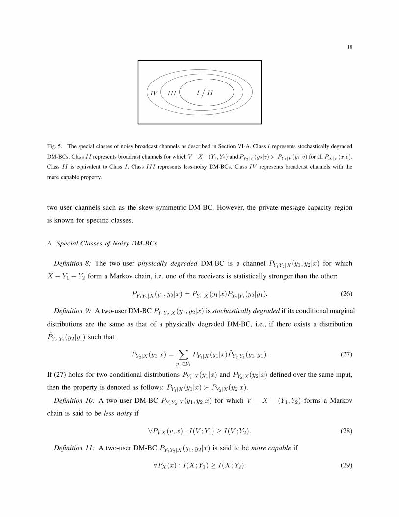
I/
IIIIIIV
Fig. 5. The special classes of noisy broadcast channels as described in Section VI-A. Class I represents stochastically degraded
DM-BCs. Class II represents broadcast channels for which V −X−(Y1, Y2) and PY2|V (y2|v) ≻ PY1|V (y1|v) for all PX|V (x|v).
Class II is equivalent to Class I . Class III represents less-noisy DM-BCs. Class IV represents broadcast channels with the
more capable property.
two-user channels such as the skew-symmetric DM-BC. However, the private-message capacity region
is known for specific classes.
A. Special Classes of Noisy DM-BCs
Definition 8: The two-user physically degraded DM-BC is a channel PY1Y2|X(y1, y2|x) for which
X − Y1 − Y2 form a Markov chain, i.e. one of the receivers is statistically stronger than the other:
PY1Y2|X(y1, y2|x) = PY1|X(y1|x)PY2|Y1(y2|y1). (26)
Definition 9: A two-user DM-BC PY1Y2|X(y1, y2|x) is stochastically degraded if its conditional marginal
distributions are the same as that of a physically degraded DM-BC, i.e., if there exists a distribution
PY2|Y1(y2|y1) such that
PY2|X(y2|x) =∑
y1∈Y1
PY1|X(y1|x)PY2|Y1(y2|y1). (27)
If (27) holds for two conditional distributions PY1|X(y1|x) and PY2|X(y2|x) defined over the same input,
then the property is denoted as follows: PY1|X(y1|x) ≻ PY2|X(y2|x).
Definition 10: A two-user DM-BC PY1Y2|X(y1, y2|x) for which V − X − (Y1, Y2) forms a Markov
chain is said to be less noisy if
∀PV X(v, x) : I(V ;Y1) ≥ I(V ;Y2). (28)
Definition 11: A two-user DM-BC PY1Y2|X(y1, y2|x) is said to be more capable if
∀PX(x) : I(X;Y1) ≥ I(X;Y2). (29)
19
The following lemma relates the properties of the special classes of noisy broadcast channels. A more
comprehensive treatment of special classes is given by C. Nair in [36].
Lemma 3: Consider a two-user DM-BC PY1Y2|X(y1, y2|x). Let V −X−(Y1, Y2) form a Markov chain,
|V| > 1, and PV (v) > 0. The following implications hold:
X − Y1 − Y2
⇒ PY1|X(y1|x) ≻ PY2|X(y2|x) (30)
⇔ ∀PX|V (x|v) : PY1|V (y1|v) ≻ PY2|V (y2|v) (31)
⇒ ∀PV X(v, x) : I(V ;Y1) ≥ I(V ;Y2) (32)
⇒ ∀PX(x) : I(X;Y1) ≥ I(X;Y2). (33)
The converse statements for (30), (32), and (33) do not hold in general. Figure 5 illustrates the different
types of broadcast channels as a hierarchy.
Proof: See Section E of the Appendices.
B. Cover’s Inner Bound
Superposition coding involves one auxiliary random variable V which conveys a “cloud center” or a
coarse message decoded by both receivers [1]. One of the receivers then decodes an additional “satellite
codeword” conveyed through X containing a fine-grain message that is superimposed upon the coarse
information.
Proposition 4 (Cover’s Inner Bound): For any two-user DM-BC, the rates (R1, R2) ∈ R2+ are achiev-
able in the region R(X,V, Y1, Y2) where
R(X,V, Y1, Y2) ,
R1, R2
∣
∣
∣R1 ≤ I(X;Y1|V ),
R2 ≤ I(V ;Y2),
R1 +R2 ≤ I(X;Y1)
. (34)
and where random variables X,V, Y1, Y2 obey the Markov chain V −X − (Y1, Y2).
Remark 7: Cover’s inner bound is applicable for any broadcast channel. By symmetry, the following
rate region is also achievable: R1, R2 | R2 ≤ I(X;Y2|V ), R1 ≤ I(V ;Y1), R1 + R2 ≤ I(X;Y2) for
random variables obeying the Markov chain V −X − (Y1, Y2).
Remark 8: The inner bound is the capacity region for degraded, less-noisy, and more-capable DM-BCs
(i.e. Class I through Class IV as shown in Figure 5). For the degraded and less-noisy special classes,

20
0
1
0
1
0
1
X
Y1
Y2
b
b
b
b
b
b
1− p1
p1
1− p2
p2
0 0.2 0.4 0.6 0.8 10
0.2
0.4
0.6
0.8
1
R1
R2
Capacity Region: p1 = 1
100, p2 = 1
10
Fig. 6. DM-BC with BSCs: The classic two-user broadcast channel consisting of a BSC(p1 = 1100
) and a BSC(p2 = 110
). The
private-message capacity region is equivalent to the superposition coding inner bound. For a fixed auxiliary and input distribution
PV X(v, x), the superposition inner bound is plotted as a rectangle in R2+ for α = 1
10and α = 1
4as described in Example 2.
For this example, polar codes achieve all points on the capacity boundary.
the capacity region is simplified to R1, R2 | R1 ≤ I(X;Y1|V ), R2 ≤ I(V ;Y2). To see this, note
that I(V ;Y2) ≤ I(V ;Y1) which implies I(V ;Y2) + I(X;Y1|V ) ≤ I(V ;Y1) + I(X;Y1|V ) = I(X;Y1).
Therefore the sum-rate constraint R1+R2 ≤ I(X;Y1) of the rate-region in (34) is automatically satisfied.
Example 2 (Binary Symmetric DM-BC): The two-user binary symmetric DM-BC consists of a binary
symmetric channel with flip probability p1 denoted as BSC(p1) and a second channel BSC(p2). Assume
that p1 < p2 < 12 which implies stochastic degradation as defined in (27). For α ∈ [0, 12 ], Cover’s
superposition inner bound is the region,
R1, R2
∣
∣
∣R1 ≤ hb(α ∗ p1)− hb(p1),
R2 ≤ 1− hb(α ∗ p2)
(35)
The above inner bound is determined by evaluating (34) where V is a Bernoulli random variable with
PV (v) = 12 , X = V ⊕ S, and S is a Bernoulli random variable with PS(1) = α. Figure 6 plots this
rectangular inner bound for two different values α = 110 and α = 1
4 . The corner points of this rectangle
given in (35) lie on the capacity boundary.
Example 3 (DM-BC with BEC(ǫ) and BSC(p) [36]): Consider a two-user DM-BC comprised of a
BSC(p) from X to Y1 and a BEC(ǫ) from X to Y2. Then it can be shown that the following cases hold:
• 0 < ǫ ≤ 2p: Y1 is degraded with respect to Y2.
• 2p < ǫ ≤ 4p(1− p): Y2 is less noisy than Y1 but Y1 is not degraded with respect to Y2.

21
• 4p(1 − p) < ǫ ≤ hb(p): Y2 is more capable than Y1 but not less noisy.
• hb(p) < ǫ < 1: The channel does not belong to the special classes.
The capacity region for all channel parameters for this example is achieved using superposition coding.
C. Main Result
Theorem 2 (Polarization-Based Superposition Code): Consider any two-user DM-BC with binary in-
put alphabet X = 0, 1 and arbitrary output alphabets Y1, Y2. There exists a sequence of polar broadcast
codes over n channel uses which achieves the following rate region
R(V,X, Y1, Y2) ,
R1, R2
∣
∣
∣R1 ≤ I(X;Y1|V ),
R2 ≤ I(V ;Y2)
, (36)
where random variables V,X, Y1, Y2 have the following listed properties:
• V is a binary random variable.
• PY1|V (y1|v) ≻ PY2|V (y2|v).
• V −X − (Y1, Y2) form a Markov chain.
For 0 < β < 12 , the average error probability of this code sequence decays as P
(n)e = O(2−n
β
). The
complexity of encoding and decoding is O(n log n).
Remark 9: The requirement that auxiliary V is a binary random variable is due to the use of binary
polarization theorems in the proof. Indeed, the auxiliary V may need to have a larger alphabet in the case
of broadcast channels. An extension to q-ary random variables is entirely possible if q-ary polarization
theorems are utilized.
Remark 10: The requirement that V−X−(Y1, Y2) holds is standard for superposition coding over noisy
channels. However, the listed property PY1|V (y1|v) ≻ PY2|V (y2|v) is due to the structure of polarization
and is used in the proof to guarantee that polarization indices are aligned. If both receivers are able to
decode the coarse message carried by the auxiliary random variable V , the polarization indices for the
coarse message must be nested for the two receivers’ channels.
VII. PROOF OF THEOREM 2
The block diagram for polarization-based superposition coding is given in Figure 7. Similar to random
codes in Shannon theory, polarization-based codes rely on n-length i.i.d. statistics of random variables;
however, a specific polarization structure based on the chain rule of entropy allows for efficient encoding

22
Xn
PY1Y2|X(y1, y2|x)
D2
Y n1
Y n2
W1W1
W2Gn
W2 V n
D1
Un2E2
E1 Gn
Un1
Fig. 7. Block diagram of a polarization-based superposition code for a two-user noisy broadcast channel.
and decoding. The key idea of Cover’s inner bound is to superimpose two messages of information onto
one codeword.
A. Polar Transform
Consider the i.i.d. sequence of random variables (V j ,Xj , Y j1 , Y
j2 ) ∼ PV (v)PX|V (x|v)PY1Y2|X(y1, y2|x)
where the index j ∈ [n]. Let the n-length sequence of auxiliary and input variables (V j ,Xj) be organized
into the random matrix
Ω ,
X1 X2 X3 . . . Xn
V 1 V 2 V 3 . . . V n
. (37)
Applying the polar transform to Ω results in the random matrix U , ΩGn. Let the random variables in
the random matrix U be indexed as follows:
U =
U11 U2
1 U31 . . . Un1
U12 U2
2 U32 . . . Un2
. (38)
The above definitions are consistent with the block diagram given in Figure 7 (and noting that Gn = G−1n ).
The polar transform extracts the randomness of Ω. In the transformed domain, the joint distribution of
the random variables in U is given by
PUn1 U
n2
(
un1 , un2
)
, PXnV n
(
un1Gn, un2Gn
)
. (39)
For polar coding purposes, the joint distribution is decomposed as follows,
PUn1 U
n2
(
un1 , un2
)
= PUn2(un2 )PUn
1 |Un2
(
un1∣
∣un2)
=
n∏
j=1
P(
u2(j)∣
∣u1:j−12
)
P(
u1(j)∣
∣u1:j−11 , un2
)
. (40)
The conditional distributions may be computed efficiently using recursive protocols as already mentioned.
The polarized variables in U are not i.i.d. random variables.

23
B. Polarization Theorems Revisited
Definition 12 (Polarization Sets for Superposition Coding): Let V n,Xn, Y n1 , Y
n2 be the sequence of
random variables as introduced in Section VII-A. In addition, let Un1 = XnGn and Un2 = V n
Gn. Let
δn = 2−nβ
for 0 < β < 12 . The following polarization sets are defined:
H(n)X|V ,
j ∈ [n] : Z(
U1(j)∣
∣
∣U1:j−11 , V n
)
≥ 1− δn
,
L(n)X|V Y1
,
j ∈ [n] : Z(
U1(j)∣
∣
∣U1:j−11 , V n, Y n
1
)
≤ δn
,
L(n)V |Y1
,
j ∈ [n] : Z(
U2(j)∣
∣
∣U1:j−12 , Y n
1
)
≤ δn
.
H(n)V ,
j ∈ [n] : Z(
U2(j)∣
∣
∣U1:j−12
)
≥ 1− δn
,
L(n)V |Y2
,
j ∈ [n] : Z(
U2(j)∣
∣
∣U1:j−12 , Y n
2
)
≤ δn
.
Definition 13 (Message Sets for Superposition Coding): In terms of the polarization sets given in Def-
inition 12, the following message sets are defined:
M(n)1v , H
(n)V ∩ L
(n)V |Y1
, (41)
M(n)1 , H
(n)X|V ∩ L
(n)X|V Y1
. (42)
M(n)2 , H
(n)V ∩ L
(n)V |Y2
. (43)
Proposition 5 (Polarization): Consider the polarization sets given in Definition 12 and the message
sets given in Definition 13 with parameter δn = 2−nβ
for 0 < β < 12 . Fix a constant τ > 0. Then there
exists an No = No(β, τ) such that
1
n
∣
∣
∣M
(n)1
∣
∣
∣≥
(
H(X|V )−H(X|V, Y1))
−τ, (44)
1
n
∣
∣
∣M
(n)2
∣
∣
∣≥
(
H(V )−H(V |Y2))
−τ, (45)
for all n > No.
Lemma 4: Consider the message sets defined in Definition 13. If the property PY1|V (y1|v) ≻ PY2|V (y2|v)
holds for conditional distributions PY1|V (y1|v) and PY2|V (y2|v), then the Bhattacharyya parameters
Z(
U2(j)∣
∣
∣U1:j−12 , Y n
1
)
≤ Z(
U2(j)∣
∣
∣U1:j−12 , Y n
2
)
for all j ∈ [n]. As a result,
M(n)2 ⊆ M
(n)1v .

24
Proof: The proof follows from Lemma 12 and repeated application of Lemma 13 in Appendix A.
C. Broadcast Encoding Blocks: (E1, E2)
The polarization theorems of the previous section are useful for defining a multi-user communication
system as diagrammed in Figure 7. The broadcast encoder must map two independent messages (W1,W2)
uniformly distributed over [2nR1 ] × [2nR2 ] to a codeword xn ∈ X n in such a way that the decoding at
each separate receiver is successful. The achievable rates for a particular block length n are
R1 =1
n
∣
∣
∣M
(n)1
∣
∣
∣,
R2 =1
n
∣
∣
∣M
(n)2
∣
∣
∣.
To construct a codeword, the encoder first produces two binary sequences un1 ∈ 0, 1n and un2 ∈
0, 1n. To determine u1(j) for j ∈ M(n)1 , the bit is selected as a uniformly distributed message bit
intended for the first receiver. To determine u2(j) for j ∈ M(n)2 , the bit is selected as a uniformly
distributed message bit intended for the second receiver. The remaining non-message indices of un1 and
un2 are computed according to deterministic or random functions which are shared between the encoder
and decoder.
1) Deterministic Mapping: Consider the following deterministic boolean functions indexed by j ∈ [n]:
ψ(j)1 : 0, 1n+j−1 → 0, 1, (46)
ψ(j)2 : 0, 1j−1 → 0, 1. (47)
As an example, consider the deterministic boolean functions based on the maximum a posteriori polar
coding rule.
ψ(j)1
(
u1:j−11 , vn
)
, argmaxu∈0,1
P
(
U1(j) = u∣
∣
∣U1:j−11 = u1:j−1
1 , V n = vn)
. (48)
ψ(j)2
(
u1:j−12
)
, argmaxu∈0,1
P
(
U2(j) = u∣
∣
∣U1:j−12 = u1:j−1
2
)
. (49)
2) Random Mapping: Consider the following class of random boolean functions indexed by j ∈ [n]:
Ψ(j)1 : 0, 1n+j−1 → 0, 1, (50)
Ψ(j)2 : 0, 1j−1 → 0, 1. (51)
25
As an example, consider the random boolean functions
Ψ(j)1
(
u1:j−11 , vn
)
,
0, w.p. λ0(
u1:j−11 , vn
)
,
1, w.p. 1− λ0(
u1:j−11 , vn
)
,
(52)
Ψ(j)2
(
u1:j−12
)
,
0, w.p. λ0(
u1:j−12
)
,
1, w.p. 1− λ0(
u1:j−12
)
,
(53)
where
λ0(
u1:j−12
)
, P(
U2(j) = 0∣
∣U1:j−12 = u1:j−1
2
)
.
λ0(
u1:j−11 , vn
)
, P(
U1(j) = 0∣
∣U1:j−11 = u1:j−1
1 , V n = vn)
.
The random boolean functions Ψ(j)1 and Ψ
(j)2 may be thought of as a vector of independent Bernoulli
random variables indexed by the input to the function. Each Bernoulli random variable of the vector is
zero or one with a fixed probability.
3) Protocol: The encoder constructs the sequence un2 first using the message bits W2 and either (49)
or (53). Next, the sequence vn = un2Gn is created. Finally, the sequence un1 is constructed using the
message bits W1, the sequence vn, and either the deterministic maps defined in (48) or the randomized
maps in (52). The transmitted codeword is xn = un1Gn.
D. Broadcast Decoding Based on Polarization
1) Decoding At First Receiver: Decoder D1 decodes the binary sequence un2 first using its observations
yn1 . It then reconstructs vn = un2Gn. Using the sequence vn and observations yn1 , the decoder reconstructs
un1 . The message W1 is located at the indices j ∈ M(n)1 in the sequence un1 . More precisely, define the
following deterministic polar decoding functions:
ξ(j)v
(
u1:j−12 , yn1
)
, argmaxu∈0,1
P
(
U2(j) = u∣
∣
∣U1:j−12 = u1:j−1
2 , Y n1 = yn1
)
. (54)
ξ(j)u1
(
u1:j−11 , vn, yn1
)
, argmaxu∈0,1
P
(
U1(j) = u∣
∣
∣U1:j−11 = u1:j−1
1 , V n = vn, Y n1 = yn1
)
. (55)
The decoder D1 reconstructs un2 bit-by-bit successively as follows using the identical shared random
mapping Ψ(j)2 (or possibly the identical shared mapping ψ
(j)2 ) used at the encoder:
u2(j) =
ξ(j)v
(
u1:j−12 , yn1
)
, if j ∈ M(n)2 ,
Ψ(j)2
(
u1:j−12
)
, otherwise.
(56)

26
If Lemma 4 holds, note that M(n)2 ⊆ M
(n)1v . With un2 , decoder D1 reconstructs vn = un2Gn. Then the
sequence un1 is constructed bit-by-bit successively as follows using the identical shared random mapping
Ψ(j)1 (or possibly the identical shared mapping ψ
(j)1 ) used at the encoder:
u1(j) =
ξ(j)u1
(
u1:j−11 , vn, yn1
)
, if j ∈ M(n)1 ,
Ψ(j)1
(
u1:j−11 , vn
)
, otherwise.
(57)
2) Decoding At Second Receiver: The decoder D2 decodes the binary sequence un2 using observations
yn2 . The message W2 is located at the indices j ∈ M(n)2 of the sequence un2 . More precisely, define the
following polar decoding functions
ξ(j)v
(
u1:j−12 , yn2
)
, argmaxu∈0,1
P
(
U2(j) = u∣
∣
∣U1:j−12 = u1:j−1
2 , Y n2 = yn2
)
. (58)
The decoder D2 reconstructs un2 bit-by-bit successively as follows using the identical shared random
mapping Ψ(j)2 (or possibly the identical shared mapping ψ
(j)2 ) used at the encoder:
u2(j) =
ξ(j)v
(
u1:j−12 , yn2
)
, if j ∈ M(n)2 ,
Ψ(j)2
(
u1:j−12
)
, otherwise.
(59)
Remark 11: The encoder and decoders execute the same protocol for reconstructing bits at the non-
message indices. This is achieved by applying the same deterministic maps ψ(j)1 and ψ
(j)2 or randomized
maps Ψ(j)1 and Ψ
(j)2 .
E. Total Variation Bound
To analyze the average probability of error P(n)e via the probabilistic method, it is assumed that both
the encoder and decoder share the randomized mappings Ψ(j)1 and Ψ
(j)2 . Define the following probability
measure on the space of tuples of binary sequences.
Q(
un1 , un2
)
, Q(
un2)
Q(
un1∣
∣un2)
=
n∏
j=1
Q(
u2(j)∣
∣
∣u1:j−12
)
Q(
u1(j)∣
∣
∣u1:j−11 , un2
)
. (60)
In (60), the conditional probability measures are defined as
Q(
u2(j)∣
∣
∣u1:j−12
)
,
12 , if j ∈ M
(n)2 ,
P(
u2(j)∣
∣
∣u1:j−12
)
, otherwise.
Q(
u1(j)∣
∣
∣u1:j−11 , un2
)
,
12 , if j ∈ M
(n)1 ,
P(
u1(j)∣
∣
∣u1:j−11 , un2
)
, otherwise.

27
The probability measureQ defined in (60) is a perturbation of the joint probability measure PUn1 U
n2(un1 , u
n2 )
in (40). The only difference in definition between P and Q is due to those indices in message sets M(n)1
and M(n)2 . The following lemma provides a bound on the total variation distance between P and Q. The
lemma establishes the fact that inserting uniformly distributed message bits in the proper indices M(n)1
and M(n)2 at the encoder does not perturb the statistics of the n-length random variables too much.
Lemma 5: (Total Variation Bound) Let probability measures P and Q be defined as in (40) and (60)
respectively. Let 0 < β < 1. For sufficiently large n, the total variation distance between P and Q is
bounded as
∑
un1∈0,1
n
un2∈0,1
n
∣
∣
∣PUn
1 Un2
(
un1 , un2
)
−Q(
un1 , un2
)
∣
∣
∣≤ 2−n
β
.
Proof: See Section C of the Appendices.
F. Error Sequences
The decoding protocols for D1 and D2 were established in Section VII-D. To analyze the probability of
error of successive cancelation (SC) decoding, consider the sequences un1 and un2 formed at the encoder,
and the resulting observations yn1 and yn2 received by the decoders. It is convenient to group the sequences
together and consider all tuples (un1 , un2 , y
n1 , y
n2 ).
Decoder D1 makes an SC decoding error on the j-th bit for the following tuples:
T j1v ,
(
un1 , un2 , y
n1 , y
n2
)
:
PUj
2
∣
∣U1:j−12 Y n
1
(
u2(j)∣
∣u1:j−12 , yn1
)
≤
PUj
2
∣
∣U1:j−12 Y n
1
(
u2(j)⊕ 1∣
∣u1:j−12 , yn1
)
,
T j1 ,
(
un1 , un2 , y
n1 , y
n2
)
:
PUj
1
∣
∣U1:j−11 V nY n
1
(
u1(j)∣
∣u1:j−11 , un2Gn, y
n1
)
≤
PUj
1
∣
∣U1:j−11 V nY n
1
(
u1(j) ⊕ 1∣
∣u1:j−11 , un2Gn, y
n1
)
. (61)
The set T j1v represents those tuples causing an error at D1 in the case u2(j) is inconsistent with respect to
observations yn1 and the decoding rule. The set T j1 represents those tuples causing an error at D1 in the
case u1(j) is inconsistent with respect to vn = un2Gn, observations yn1 , and the decoding rule. Similarly,

28
decoder D2 makes an SC decoding error on the j-th bit for the following tuples:
T j2 ,
(
un1 , un2 , y
n1 , y
n2
)
: PU2
∣
∣U1:j−12 Y n
2
(
u2∣
∣u1:j−12 , yn2
)
≤
PU2
∣
∣U1:j−12 Y n
2
(
u2 ⊕ 1∣
∣u1:j−12 , yn2
)
.
The set T j2 represents those tuples causing an error at D2 in the case u2(j) is inconsistent with respect
to observations yn2 and the decoding rule. Since both decoders D1 and D2 only declare errors for those
indices in the message sets, the set of tuples causing an error is
T1v ,⋃
j∈M(n)2 ⊆M(n)
1v
T j1v, (62)
T1 ,⋃
j∈M(n)1
T j1 , (63)
T2 ,⋃
j∈M(n)2
T j2 . (64)
The complete set of tuples causing a broadcast error is
T , T1v ∪ T1 ∪ T2. (65)
The goal is to show that the probability of choosing tuples of error sequences in the set T is small under
the distribution induced by the broadcast code.
G. Average Error Probability
Denote the total sum rate of the broadcast protocol as RΣ = R1 +R2. Consider first the use of fixed
deterministic maps ψ(j)1 and ψ
(j)2 shared between the encoder and decoders. Then the probability of error
of broadcasting the two messages at rates R1 and R2 is given by
P (n)e
[
ψ(j)1 , ψ
(j)2
]
=∑
un1 ,u
n2 ,y
n1 ,y
n2 ∈T
[
PY n1 Y
n2
∣
∣Un1 U
n2
(
yn1 , yn2
∣
∣un1 , un2
)
·1
2nR2
∏
j∈[n]:j/∈M(n)2
1[ψ(j)2 (u1:j−1
2 )=u2(j)]
·1
2nR1
∏
j∈[n]:j/∈M(n)1
1[ψ(j)1 (u1:j−1
1 ,un2Gn)=u1(j)]
]
.

29
If the encoder and decoders share randomized maps Ψ(j)1 and Ψ
(j)2 , then the average probability of
error is a random quantity determined as follows
P (n)e
[
Ψ(j)1 ,Ψ
(j)2
]
=∑
un1 ,u
n2 ,y
n1 ,y
n2 ∈T
[
PY n1 Y
n2
∣
∣Un1 U
n2
(
yn1 , yn2
∣
∣un1 , un2
)
·1
2nR2
∏
j∈[n]:j/∈M(n)2
1[Ψ(j)2 (u1:j−1
2 )=u2(j)]
·1
2nR1
∏
j∈[n]:j/∈M(n)1
1[Ψ(j)1 (u1:j−1
1 ,un2Gn)=u1(j)]
]
.
By averaging over the randomness in the encoders and decoders, the expected block error probability is
upper bounded in the following lemma.
Lemma 6: Consider the polarization-based superposition code described in Section VII-C and Sec-
tion VII-D. Let R1 and R2 be the broadcast rates selected according to the Bhattacharyya criterion given
in Proposition 5. Then for 0 < β < 1 and sufficiently large n,
EΨ(j)1 ,Ψ(j)
2
[
P (n)e [Ψ
(j)1 ,Ψ
(j)2 ]
]
< 2−nβ
.
Proof: See Section C of the Appendices.
If the average probability of error decays to zero in expectation over the random maps Ψ(j)1 and Ψ
(j)2 ,
then there must exist at least one fixed set of maps for which P(n)e → 0.
VIII. NOISY BROADCAST CHANNELS
MARTON’S CODING SCHEME
A. Marton’s Inner Bound
For general noisy broadcast channels, Marton’s inner bound involves two correlated auxiliary random
variables V1 and V2 [3]. The intuition behind the coding strategy is to identify two “virtual” channels,
one from V1 to Y1, and the other from V2 to Y2. Somewhat surprisingly, although the broadcast messages
are independent, the auxiliary random variables V1 and V2 may be correlated to increase rates to both
receivers. While there exist generalizations of Marton’s strategy, the basic version of the inner bound is
presented in this section3.
3In addition, it is difficult even to evaluate Marton’s inner bound for general channels due to the need for proper cardinality
bounds on the auxiliaries [37]. These issues lie outside the scope of the present paper.

30
Gn
Xn
PY1Y2|X(y1, y2|x)
D2
Y n1
Y n2
W1 W1
W2Gn
W2
x = φ(v1, v2)
V n1
V n2
D1Un1
Un2
E1
E2
Fig. 8. Block diagram of a polarization-based Marton code for a two-user noisy broadcast channel.
Proposition 6 (Marton’s Inner Bound): For any two-user DM-BC, the rates (R1, R2) ∈ R2+ in the
pentagonal region R(X,V1, V2, Y1, Y2) are achievable where
R(X,V1, V2, Y1, Y2) ,
R1, R2
∣
∣
∣R1 ≤ I(V1;Y1),
R2 ≤ I(V2;Y2),
R1 +R2 ≤ I(V1;Y1) + I(V2;Y2)− I(V1;V2)
. (66)
and whereX,V1, V2, Y1, Y2 have a joint distribution given by PV1V2(v1, v2)PX|V1V2
(x|v1, v2)PY1Y2|X(y1, y2|x).
Remark 12: It can be shown that for Marton’s inner bound there is no loss of generality if PX|V1V2(x|v1, v2) =1[x=φ(v1,v2)] where φ(v1, v2) is a deterministic function [2, Section 8.3]. Thus, by allowing a larger
alphabet size for the auxiliaries, X may be a deterministic function of auxiliaries (V1, V2). Marton’s
inner bound is tight for the class of semi-deterministic DM-BCs for which one of the outputs is a
deterministic function of the input.
B. Main Result
Theorem 3 (Polarization-Based Marton Code): Consider any two-user DM-BC with arbitrary input
and output alphabets. There exist sequences of polar broadcast codes over n channel uses which achieve
the following rate region
R(V1, V2,X, Y1, Y2) ,
R1, R2
∣
∣
∣R1 ≤ I(V1;Y1),
R2 ≤ I(V2;Y2)− I(V1;V2)
, (67)
where random variables V1, V2,X, Y1, Y2 have the following listed properties:
• V1 and V2 are binary random variables.

31
• PY2|V2(y2|v2) ≻ PV1|V2
(v1|v2).
• For a deterministic function φ : 0, 12 → X , the joint distribution of all random variables is given
by
PV1V2XY1Y2(v1, v2, x, y1, y2) = PV1V2
(v1, v2)1[x=φ(v1,v2)]PY1Y2|X(y1, y2|x).
For 0 < β < 12 , the average error probability of this code sequence decays as P
(n)e = O(2−n
β
). The
complexity of encoding and decoding is O(n log n).
Remark 13: The listed property PY2|V2(y2|v2) ≻ PV1|V2
(v1|v2) is necessary in the proof due to polarization-
based codes requiring an alignment of polarization indices. The property is a natural restriction since it
also implies that I(Y2;V2) > I(V1;V2) so that R2 > 0. However, certain joint distributions on random
variables are not permitted using the analysis of polarization presented here. It is not clear whether a
different approach obviates the need for an alignment of indices.
Remark 14: By symmetry, the rate tuple (R1, R2) = (I(V1;Y1) − I(V1;V2), I(V2, Y2)) is achievable
with low-complexity codes under similar constraints on the joint distribution of V1, V2,X, Y1, Y2. The
rate tuple is a corner point of the pentagonal rate region of Marton’s inner bound given in (66).
IX. PROOF OF THEOREM 3
The block diagram for polarization-based Marton coding is given in Figure 8. Marton’s strategy differs
form Cover’s superposition coding with the presence of two auxiliaries and the function φ(v1, v2) which
forms the codeword symbol-by-symbol. The polar transform is applied to each n-length i.i.d. sequence
of auxiliary random variables.
A. Polar Transform
Consider the i.i.d. sequence of random variables
(V j1 , V
j2 ,X
j , Y j1 , Y
j2 ) ∼ PV1V2
(v1, v2)PX|V1V2(x|v1, v2)PY1Y2|X(y1, y2|x),
where the index j ∈ [n]. For the particular coding strategy analyzed in this section, PX|V1V2(x|v1, v2) =1[x=φ(v1,v2)]. Let the n-length sequence of auxiliary variables (V j
1 , Vj2 ) be organized into the random
matrix
Ω ,
V 11 V 2
1 V 31 . . . V n
1
V 12 V 2
2 V 32 . . . V n
2
. (68)

32
Applying the polar transform to Ω results in the random matrix U , ΩGn. Index the random variables
of U as follows:
U =
U11 U2
1 U31 . . . Un1
U12 U2
2 U32 . . . Un2
. (69)
The above definitions are consistent with the block diagram given in Figure 8 (and noting that Gn = G−1n ).
The polar transform extracts the randomness of Ω. In the transformed domain, the joint distribution of
the variables in U is given by
PUn1 U
n2
(
un1 , un2
)
, PV n1 V
n2
(
un1Gn, un2Gn
)
. (70)
However, for polar coding purposes, the joint distribution is decomposed as follows,
PUn1 U
n2
(
un1 , un2
)
= PUn1(un1 )PUn
2 |Un1
(
un2∣
∣un1)
=
n∏
j=1
P(
u1(j)∣
∣u1:j−11
)
P(
u2(j)∣
∣u1:j−12 , un1
)
. (71)
The above conditional distributions may be computed efficiently using recursive protocols. The polarized
random variables of U do not have an i.i.d. distribution.
B. Effective Channel
Marton’s achievable strategy establishes virtual channels for the two receivers via the function φ(v1, v2).
The virtual channel is given by
P φY1Y2|V1V2
(
y1, y2
∣
∣
∣v1, v2
)
, PY1Y2|X
(
y1, y2
∣
∣
∣φ(
v1, v2)
)
.
Due to the memoryless property of the DM-BC, the effective channel between auxiliaries and channel
outputs is given by
P φY n1 Y
n2 |V n
1 Vn2
(
yn1 , yn2
∣
∣
∣vn1 , v
n2
)
,
n∏
i=1
PY1Y2|X
(
y1(i), y2(i)∣
∣
∣φ(
v1(i), v2(i))
)
.
The polarization-based Marton code establishes a different effective channel between polar-transformed
auxiliaries and the channel outputs. The effective polarized channel is
P φY n1 Y
n2 |Un
1 Un2
(
yn1 , yn2
∣
∣
∣un1 , u
n2
)
P φY n1 Y
n2 |V n
1 Vn2
(
yn1 , yn2
∣
∣
∣un1Gn, u
n2Gn
)
. (72)

33
n
Z(
U2(j)∣
∣
∣U1:j−12 , V n
1
)
≥ 1− δn
δn < Z(
U2(j)∣
∣
∣U1:j−12 , V n
1
)
< 1− δn
Z(
U2(j)∣
∣
∣U1:j−12 , V n
1
)
≤ δn
n
δn < Z(
U2(j)∣
∣
∣U1:j−12 , Y n
2
)
< 1− δn
Z(
U2(j)∣
∣
∣U1:j−12 , Y n
2
)
≤ δn Z(
U2(j)∣
∣
∣U1:j−12 , Y n
2
)
≥ 1− δn
Fig. 9. The alignment of polarization indices for Marton coding over noisy broadcast channels with respect to the second
receiver. The message set M(n)2 is highlighted by the vertical red rectangles. At finite code length n, exact alignment is not
possible due to partially-polarized indices pictured in gray.
C. Polarization Theorems Revisited
Definition 14 (Polarization Sets for Marton Coding): Let V n1 , V
n2 ,X
n, Y n1 , Y
n2 be the sequence of ran-
dom variables as introduced in Section IX-A. In addition, let Un1 = V n1 Gn and Un2 = V n
2 Gn. Let
δn = 2−nβ
for 0 < β < 12 . The following polarization sets are defined:
H(n)V1
,
j ∈ [n] : Z(
U1(j)∣
∣
∣U1:j−11
)
≥ 1− δn
,
L(n)V1|Y1
,
j ∈ [n] : Z(
U1(j)∣
∣
∣U1:j−11 , Y n
1
)
≤ δn
,
H(n)V2|V1
,
j ∈ [n] : Z(
U2(j)∣
∣
∣U1:j−12 , V n
1
)
≥ 1− δn
,
L(n)V2|V1
,
j ∈ [n] : Z(
U2(j)∣
∣
∣U1:j−12 , V n
1
)
≤ δn
,
H(n)V2|Y2
,
j ∈ [n] : Z(
U2(j)∣
∣
∣U1:j−12 , Y n
2
)
≥ 1− δn
,
L(n)V2|Y2
,
j ∈ [n] : Z(
U2(j)∣
∣
∣U1:j−12 , Y n
2
)
≤ δn
.
Definition 15 (Message Sets for Marton Coding): In terms of the polarization sets given in Defini-

34
tion 14, the following message sets are defined:
M(n)1 , H
(n)V1
∩ L(n)V1|Y1
, (73)
M(n)2 , H
(n)V2|V1
∩ L(n)V2|Y2
. (74)
Proposition 7 (Polarization): Consider the polarization sets given in Definition 14 and the message
sets given in Definition 15 with parameter δn = 2−nβ
for 0 < β < 12 . Fix a constant τ > 0. Then there
exists an No = No(β, τ) such that
1
n
∣
∣
∣M
(n)1
∣
∣
∣≥
(
H(V1)−H(V1|Y1))
−τ, (75)
1
n
∣
∣
∣M
(n)2
∣
∣
∣≥
(
H(V2|V1)−H(V2|Y2))
−τ, (76)
for all n > No.
Lemma 7: Consider the polarization sets defined in Proposition 7. If the property PY2|V2(y2|v2) ≻
PV1|V2(v1|v2) holds for conditional distributions PY2|V2
(y2|v2) and PV1|V2(v1|v2), then I(V2;Y2) > I(V1;V2)
and the Bhattacharyya parameters
Z(
U2(j)∣
∣
∣U1:j−12 , Y n
2
)
≤ Z(
U2(j)∣
∣
∣U1:j−12 , V n
1
)
for all j ∈ [n]. As a result,
L(n)V2|V1
⊆ L(n)V2|Y2
,
H(n)V2|Y2
⊆ H(n)V2|V1
.
Proof: The proof follows from Lemma 12 and repeated application of Lemma 13 in Appendix A.
Remark 15: The alignment of polarization indices characterized by Lemma 7 is diagrammed in Fig-
ure 9. The alignment ensures the existence of polarization indices in the set M(n)2 for the message W2 to
have a positive rate R2 > 0. The indices in M(n)2 represent those bits freely set at the broadcast encoder
and simultaneously those bits that may be decoded by D2 given its observations.
D. Partially-Polarized Indices
As shown in Figure 9, for the Marton coding scheme, exact alignment of polarization indices is not
possible. However, the alignment holds for all but o(n) indices. The sets of partially-polarized indices
shown in Figure 9 are defined as follows.

35
Definition 16 (Sets of Partially-Polarized Indices):
∆1 , [n] \(
H(n)V2|V1
∪ L(n)V2|V1
)
, (77)
∆2 , [n] \(
H(n)V2|Y2
∪ L(n)V2|Y2
)
. (78)
As implied by Arıkan’s polarization theorems, the number of partially-polarized indices is negligible
asymptotically as n→ ∞. For an arbitrarily small η > 0,∣
∣∆1 ∪∆2
∣
∣
n≤ η, (79)
for all n sufficiently large enough. As will be discussed, providing these o(n) bits as “genie-given” bits
to the decoders results in a rate penalty; however, the rate penalty is negligible for sufficiently large code
lengths.
E. Broadcast Encoding Blocks: (E1, E2)
As diagrammed in Figure 8, the broadcast encoder must map two independent messages (W1,W2)
uniformly distributed over [2nR1 ] × [2nR2 ] to a codeword xn ∈ X n in such a way that the decoding at
each separate receiver is successful. The achievable rates for a particular block length n are
R1 =1
n
∣
∣
∣M
(n)1
∣
∣
∣,
R2 =1
n
∣
∣
∣M
(n)2
∣
∣
∣.
To construct a codeword, the encoder first produces two binary sequences un1 ∈ 0, 1n and un2 ∈
0, 1n. To determine u1(j) for j ∈ M(n)1 , the bit is selected as a uniformly distributed message bit
intended for the first receiver. To determine u2(j) for j ∈ M(n)2 , the bit is selected as a uniformly
distributed message bit intended for the second receiver. The remaining non-message indices of un1 and
un2 are decided randomly according to the proper statistics as will be described in this section. The
transmitted codeword is formed symbol-by-symbol via the φ function,
∀j ∈ [n] : x(j) = φ(
v1(j), v2(j))
where vn1 = un1Gn and vn2 = un2Gn. A valid codeword sequence is always guaranteed to be formed
unlike in the case of coding for deterministic broadcast channels.

36
1) Random Mapping: To fill in the non-message indices, we define the following random mappings.
Consider the following class of random boolean functions where j ∈ [n]:
Ψ(j)1 : 0, 1j−1 → 0, 1, (80)
Ψ(j)2 : 0, 1n+j−1 → 0, 1, (81)
Γ : [n] → 0, 1. (82)
More concretely, we consider the following specific random boolean functions based on the statistics
derived from polarization methods:
Ψ(j)1
(
u1:j−11
)
,
0, w.p. λ0
(
u1:j−11
)
,
1, w.p. 1− λ0
(
u1:j−11
)
,
(83)
Ψ(j)2
(
u1:j−12 , vn1
)
,
0, w.p. λ0
(
u1:j−12 , vn1
)
,
1, w.p. 1− λ0
(
u1:j−12 , vn1
)
(84)
Γ(j) ,
0, w.p. 12 ,
1, w.p. 12 ,
(85)
where
λ0
(
u1:j−11
)
, P
(
U1(j) = 0∣
∣
∣U1:j−11 = u1:j−1
1
)
.
λ0
(
u1:j−12 , vn1
)
, P
(
U2(j) = 0∣
∣
∣U1:j−12 = u1:j−1
2 , V n1 = vn1
)
.
For a fixed j ∈ [n], the random boolean functions Ψ(j)1 , Ψ
(j)2 may be thought of as a vector of independent
Bernoulli random variables indexed by the input to the function. Each Bernoulli random variable of the
vector is zero or one with a fixed well-defined probability that is efficiently computable. The random
boolean function Γ may be thought of as an n-length vector of Bernoulli(12 ) random variables.
2) Encoding Protocol: The broadcast encoder constructs the sequence un1 bit-by-bit successively,
u1(j) =
W1 message bit, if j ∈ M(n)1 ,
Ψ(j)1
(
u1:j−11
)
, otherwise.
(86)

37
The encoder then computes the sequence vn1 = un1Gn. To generate vn2 , the encoder constructs the sequence
un2 (given vn1 ) as follows,
u2(j) =
W2 message bit, if j ∈ M(n)2 ,
Γ(j), if j ∈ H(n)V2|V1
\ M(n)2 ,
Ψ(j)2
(
u1:j−12 , vn1
)
, otherwise.
(87)
Then the sequence vn2 = un2Gn. The randomness in the above encoding protocol over non-message
indices ensures that the pair of sequences (un1 , un2 ) has the correct statistics as if drawn from the joint
distribution of (Un1 , Un2 ). In the last step, the encoder transmits a codeword xn formed symbol-by-symbol:
x(j) = φ(
v1(j), v2(j))
for all j ∈ [n]. For j ∈ ∆2, where ∆2 is the set of partially-polarized indices
defined in (78), the encoder records the realization of u2(j). These indices will be provided to the second
receiver’s decoder D2 as “genie-given” bits.
F. Broadcast Decoding Based on Polarization
1) Decoding At First Receiver: Decoder D1 decodes the binary sequence un1 using its observations
yn1 . The message W1 is located at the indices j ∈ M(n)1 in the sequence un1 . More precisely, we define
the following deterministic polar decoding function for the j-th bit:
ξ(j)u1
(
u1:j−11 , yn1
)
, argmaxu∈0,1
P
(
U1(j) = u∣
∣
∣U1:j−11 = u1:j−1
1 , Y n1 = yn1
)
. (88)
Decoder D1 reconstructs un1 bit-by-bit successively as follows using the identical random mapping Ψ(j)1
at the encoder:
u1(j) =
ξ(j)u1
(
u1:j−11 , yn1
)
, if j ∈ M(n)1 ,
Ψ(j)1
(
u1:j−11
)
, otherwise.
(89)
Given that all previous bits u1:j−11 have been decoded correctly, decoder D1 makes a mistake on the j-th
bit u1(j) only if j ∈ M(n)1 . For the remaining indices, the decoder produces the same bit produced at
the encoder due to the shared random maps.
2) Decoding At Second Receiver: The decoder D2 decodes the binary sequence un2 using observations
yn2 . The message W2 is located at the indices j ∈ M(n)2 of the sequence un2 . Define the following
deterministic polar decoding functions
ξ(j)u2
(
u1:j−12 , yn2
)
, argmaxu∈0,1
P
(
U2(j) = u∣
∣
∣U1:j−12 = u1:j−1
2 , Y n2 = yn2
)
. (90)

38
Decoder D2 reconstructs un2 bit-by-bit successively as follows using the identical shared random mapping
Γ used at the encoder. Including all but o(n) of the indices,
u2(j) =
ξ(j)u2
(
u1:j−12 , yn2
)
, if j ∈ L(n)V2|Y2
,
Γ(j), if j ∈ H(n)V2|Y2
.
(91)
For those indices j ∈ ∆2 where ∆2 is the set of partially-polarized indices defined in (78), the decoder
D2 is provided with “genie-given” bits from the encoder. Thus, all bits are decoded, and D2 only makes
a successive cancelation error for those indices j ∈ L(n)V2|Y2
. Communicating the genie-given bits from
the encoder to decoder results in a rate penalty. However, since the number of genie-given bits scales
asymptotically as o(n), the rate penalty can be made arbitrarily small.
Remark 16: It is notable that decoder D2 reconstructs un2 using only the observations yn2 . At the
encoder, the sequence un2 was generated with the realization of a sequence vn1 as given in (87). However,
decoder D2 does not reconstruct the sequence vn1 . From this operational perspective, Marton’s scheme
differs crucially from Cover’s superposition scheme because there does not exist the notion of a “stronger”
receiver which reconstructs all the sequences decoded at the “weaker” receiver.
G. Total Variation Bound
To analyze the average probability of error P(n)e , it is assumed that both the encoder and decoder
share the randomized mappings Ψ(j)1 , Ψ
(j)2 , and Γ (where Ψ
(j)2 is not utilized at decoder D2). Define the
following probability measure on the space of tuples of binary sequences.
Q(
un1 , un2
)
, Q(
un1)
Q(
un1∣
∣un2)
=
n∏
j=1
Q(
u1(j)∣
∣u1:j−11
)
Q(
u2(j)∣
∣u1:j−12 , un1
)
, (92)
where the conditional probability measures are defined as
Q(
u1(j)∣
∣
∣u1:j−11
)
,
12 , if j ∈ M
(n)1 ,
P(
u1(j)∣
∣
∣u1:j−11
)
, otherwise.
Q(
u2(j)∣
∣
∣u1:j−12 , un1
)
,
12 , if j ∈ H
(n)V2|V1
,
P(
u2(j)∣
∣
∣u1:j−12 , un1
)
, otherwise.
The probability measureQ defined in (92) is a perturbation of the joint probability measure PUn1 U
n2(un1 , u
n2 )
in (71). The only difference in definition between P and Q is due to those indices in message sets M(n)1
and H(n)V2|V1
(note: M(n)2 ⊆ H
(n)V2|V1
). The following lemma provides a bound on the total variation distance

39
between P and Q. The lemma establishes the fact that inserting uniformly distributed message bits in
the proper indices M(n)1 and M
(n)2 (or the entire set H
(n)V2|V1
) at the encoder does not perturb the statistics
of the n-length random variables too much.
Lemma 8: (Total Variation Bound) Let probability measures P and Q be defined as in (71) and (92)
respectively. Let 0 < β < 1. For sufficiently large n, the total variation distance between P and Q is
bounded as
∑
un1∈0,1
n
un2∈0,1
n
∣
∣
∣PUn
1 Un2
(
un1 , un2
)
−Q(
un1 , un2
)
∣
∣
∣≤ 2−n
β
.
Proof: Omitted. The proof follows via the chain rule for KL-divergence and is identical to the
previous proofs of Lemma 1 and Lemma 5.
H. Error Sequences
The decoding protocols for D1 and D2 were established in Section IX-F. To analyze the probability of
error of successive cancelation (SC) decoding, consider the sequences un1 and un2 formed at the encoder,
and the resulting observations yn1 and yn2 received by the decoders. The effective polarized channel
P φY n1 Y
n2 |Un
1 Un2
(
yn1 , yn2
∣
∣un1 , un2
)
was defined in (72) for a fixed φ function. It is convenient to group the
sequences together and consider all tuples (un1 , un2 , y
n1 , y
n2 ).
Decoder D1 makes an SC decoding error on the j-th bit for the following tuples:
T j1 ,
(
un1 , un2 , y
n1 , y
n2
)
:
PUj
1
∣
∣U1:j−11 Y n
1
(
u1(j)∣
∣u1:j−11 , yn1
)
≤
PUj1 |U
1:j−11 Y n
1
(
u1(j) ⊕ 1∣
∣u1:j−11 , yn1
)
. (93)
The set T j1 represents those tuples causing an error at D1 in the case u1(j) is inconsistent with respect
to observations yn1 and the decoding rule. Similarly, decoder D2 makes an SC decoding error on the j-th
bit for the following tuples:
T j2 ,
(
un1 , un2 , y
n1 , y
n2
)
:
PU2
∣
∣U1:j−12 Y n
2
(
u2∣
∣u1:j−12 , yn2
)
≤
PU2
∣
∣U1:j−12 Y n
2
(
u2 ⊕ 1∣
∣u1:j−12 , yn2
)
.

40
The set T j2 represents those tuples causing an error at D2 in the case u2(j) is inconsistent with respect
to observations yn2 and the decoding rule. The set of tuples causing an error is
T1 ,⋃
j∈M(n)1
T j1 , (94)
T2 ,⋃
j∈L(n)
V2|V1
T j2 , (95)
T , T1 ∪ T2. (96)
The goal is to show that the probability of choosing tuples of error sequences in the set T is small under
the distribution induced by the broadcast code.
I. Average Error Probability
If the encoder and decoders share randomized maps Ψ(j)1 , Ψ
(j)2 , and Γ, then the average probability of
error is a random quantity determined as follows
P (n)e
[
Ψ(j)1 ,Ψ
(j)2 ,Γ
]
=∑
un1 ,u
n2 ,y
n1 ,y
n2 ∈T
[
P φY n1 Y
n2
∣
∣Un1 U
n2
(
yn1 , yn2
∣
∣un1 , un2
)
·1
2nR1
∏
j∈[n]:j /∈M(n)1
1[Ψ(j)1 (u1:j−1
1 )=u1(j)]
·1
2nR2
∏
j∈H(n)
V2|V1\M(n)
2
1[Γ(j)=u2(j)]
·∏
j∈[n]:j /∈H(n)
V2|V1
1[Ψ(j)2 (u1:j−1
2 ,un1Gn)=u2(j)]
]
.
By averaging over the randomness in the encoders and decoders, the expected block error probability is
upper bounded in the following lemma.
Lemma 9: Consider the polarization-based Marton code described in Section IX-E and Section IX-F.
Let R1 and R2 be the broadcast rates selected according to the Bhattacharyya criterion given in Propo-
sition 7. Then for 0 < β < 1 and sufficiently large n,
EΨ(j)1 ,Ψ(j)
2 ,Γ
[
P (n)e [Ψ
(j)1 ,Ψ
(j)2 ,Γ]
]
< 2−nβ
.
Proof: See Section D of the Appendices.
If the average probability of block error decays to zero in expectation over the random maps Ψ(j)1 ,
Ψ(j)2 , and Γ, then there must exist at least one fixed set of maps for which P
(n)e → 0. Hence, polar

41
codes for Marton’s inner bound exist under suitable restrictions on distributions and they achieve reliable
transmission according to the advertised rates (except for a small set of o(n) polarization indices as is
discussed next).
J. Rate Penalty Due to Partial Polarization
Lemma 9 is true assuming that decoder D2 obtains “genie-given” bits for the set of indices ∆2
defined in (78). The set ∆2 represents those indices that are partially-polarized and which cause a slight
misalignment of polarization indices in the Marton scheme. Fortunately, the set ∆2 contains a vanishing
fraction of indices: 1n
∣
∣∆2
∣
∣≤ η for η > 0 arbitrarily small and n sufficiently large. Therefore, a two-phase
strategy suffices for sending the “genie-given” bits. In the first phase of communication, the encoder sends
several n-length blocks while decoder D2 waits to decode. After accumulating several blocks of output
sequences, the encoder transmits all the known bits in the set ∆2 for all the first-phase transmissions.
The encoder and decoder can use any reliable point-to-point polar code with non-vanishing rate for
communication. Having received the “genie-aided” bits in the second-phase, the second receiver then
decodes all the first-phase blocks. The number of blocks sent in the first-phase is O( 1η ). The rate penalty
is O(η) where η can be made arbitrarily small. A similar argument was provided in [24] for designing
polar codes for the Gelfand-Pinsker problem.
X. CONCLUSION
Coding for broadcast channels is fundamental to our understanding of communication systems. Broad-
cast codes based on polarization methods achieve rates on the capacity boundary for several classes
of DM-BCs. In the case of m-user deterministic DM-BCs, polarization of random variables from the
channel output provides the ability to extract uniformly random message bits while maintaining broadcast
constraints at the encoder. As referenced in the literature, maintaining multi-user constraints for the DM-
BC is a difficult task for traditional belief propagation algorithms and LDPC codes.
For two-user noisy DM-BCs, polar codes were designed based on Marton’s coding strategy and Cover’s
superposition strategy. Constraints on auxiliary and input distributions were placed in both cases to ensure
alignment of polarization indices in the multi-user setting. The asymptotic behavior of the average error
probability was shown to be P(n)e = O(2−n
β
) with an encoding and decoding complexity of O(n log n).
The next step is to supplement the theory with experimental evidence of the error-correcting capability
of polar codes over simulated channels for finite code lengths. The results demonstrate that polar codes
have a potential for use in several network communication scenarios.

42
APPENDIX A
POLAR CODING LEMMAS
The following lemmas provide a basis for proving polar coding theorems. A subset of the lemmas
were proven in different contexts, e.g., channel vs. source coding, and contain citations to references.
Lemma 10: Consider two random variables X ∈ 0, 1 and Y ∈ Y with joint distribution PX,Y (x, y).
Let Q(x|y) = 12 denote a uniform conditional distribution for x ∈ 0, 1 and y ∈ Y . Then the following
identity holds.
D(
PX|Y (x|y)∥
∥
∥Q(x|y)
)
= 1−H(X|Y ). (97)
Proof: The identity follows from standard definitions of entropy and Kullback-Leibler distance.
H(X|Y ) =∑
y∈Y
PY (y)∑
x∈0,1
PX|Y (x|y) log21
PX|Y (x|y)
=∑
y∈Y
PY (y)∑
x∈0,1
PX|Y (x|y) log21
Q(x|y)
−∑
y∈Y
PY (y)∑
x∈0,1
PX|Y (x|y) log2PX|Y (x|y)
Q(x|y)
=∑
y∈Y
PY (y)
1−∑
x∈0,1
PX|Y (x|y) log2PX|Y (x|y)
Q(x|y)
= 1−D(
PX|Y (x|y)∥
∥
∥Q(x|y)
)
.
Lemma 11 (Estimating The Bhattacharyya Parameter): Let (T, V ) ∼ PT,V (t, v) where T ∈ 0, 1
and V ∈ V where V is an arbitrary discrete alphabet. Define a likelihood function L(v) and inverse
likelihood function L−1(v) as follows.
L(v) ,PT |V (0|v)
PT |V (1|v), L−1(v) ,
PT |V (1|v)
PT |V (0|v)
To account for degenerate cases in which PT |V (t|v) = 0, define the following function,
ϕ(t, v) ,
0 if 1[PT |V (t|v)=0]
L(v) if 1[PT |V (t|v)>0] and 1[t=1]
L−1(v) if 1[PT |V (t|v)>0] and 1[t=0]

43
In order to estimate Z(T |V ) ∈ [0, 1], it is convenient to sample from PTV (t, v) and express Z(T |V ) as
an expectation over random variables T and V ,
Z(T |V ) = ET,V
√
ϕ(T, V ). (99)
Proof: The following forms of the Bhattacharyya parameter are equivalent.
Z(T |V ) , 2∑
v∈V
PV (v)√
PT |V (0|v)PT |V (1|v)
= 2∑
v∈V
√
PTV (0, v)PTV (1, v)
=∑
v∈V
PV (v)∑
t∈0,1
√
PT |V (t|v)(1 − PT |V (t|v))
=∑
t∈0,1
∑
v:PT |V (t|v)>0v∈V
PTV (t, v)
√
1− PT |V (t|v)
PT |V (t|v)
= ET,V
√
ϕ(T, V ).
Lemma 12 (Stochastic Degradation (cf. [23])): Consider discrete random variables V , Y1, and Y2.
Assume that |V| = 2 and that discrete alphabets Y1 and Y2 have an arbitrary size. Then
PY1|V (y1|v) ≻ PY2|V (y2|v) ⇒ Z(V |Y2) ≥ Z(V |Y1). (100)
Proof: Beginning with the definition of the Bhattacharyya parameter leads to the following derivation:
Z(V |Y2) , 2∑
y2
√
PV Y2(0, y2)PV Y2
(1, y2)
= 2∑
y2
√
PV (0)PV (1)√
PY2|V (y2|0)PY2|V (y2|1)
= 2√
PV (0)PV (1)∑
y2
[
√
∑
y1
PY1|V (y1|0)PY2|Y1(y2|y1) ·
√
∑
y1
PY1|V (y1|1)PY2|Y1(y2|y1)
]
.
Then applying the Cauchy–Schwarz inequality yields
Z(V |Y2) ≥ 2√
PV (0)PV (1)∑
y2
[
∑
y1
√
PY1|V (y1|0)PY2|Y1(y2|y1) ·
∑
y1
√
PY1|V (y1|1)PY2|Y1(y2|y1)
]
= 2√
PV (0)PV (1)∑
y2
[
∑
y1
PY2|Y1(y2|y1) ·
√
PY1|V (y1|0)PY1|V (y1|1)
]
.

44
Interchanging the order of summations yields
Z(V |Y2) ≥ 2√
PV (0)PV (1)
[
∑
y1
√
PY1|V (y1|0)PY1|V (y1|1) ·∑
y2
PY2|Y1(y2|y1)
]
= Z(V |Y1).
Lemma 13 (Successive Stochastic Degradation (cf. [23])): Consider a binary random variable V , and
discrete random variables Y1 with alphabet Y1, and Y2 with alphabet Y2. Assume that the joint distribution
PV Y1Y2obeys the constraint PY1|V (y1|v) ≻ PY2|V (y2|v). Consider two i.i.d. random copies (V 1, Y 1
1 , Y12 )
and (V 2, Y 21 , Y
22 ) distributed according to PV Y1Y2
. Define two binary random variables U1 , V 1 ⊕ V 2
and U2 , V 2. Then the following holds
Z(
U1∣
∣Y 1:22
)
≥ Z(
U1∣
∣Y 1:21
)
, (101)
Z(
U2∣
∣U1, Y 1:22
)
≥ Z(
U2∣
∣U1, Y 1:21
)
. (102)
Proof: Given the assumptions, the following stochastic degradation conditions hold:
PY 11 |V 1(y11|v
1) ≻ PY 12 |V 1(y12 |v
1), (103)
PY 21 |V 2(y21|v
2) ≻ PY 22 |V 2(y22 |v
2). (104)
The goal is to derive new stochastic degradation conditions for the polarized conditional distributions.
The binary random variables U1 and U2 are not necessarily independent Bernoulli(12 ) variables. Taking
this into account,
PY 12 Y
22 |U1
(
y12, y22
∣
∣u1)
=1
PU1(u1)
∑
u2∈0,1
PV 1Y 12
(
u1 ⊕ u2, y12)
PV 2Y 22
(
u2, y22)
=1
PU1(u1)
∑
u2∈0,1
[
PY 12 |V 1
(
y12∣
∣u1 ⊕ u2)
PV 1
(
u1 ⊕ u2)
·PY 22 |V 2
(
y22∣
∣u2)
PV 2(u2)
]
.
Applying the property due to the assumption in (103),
PY 12 Y
22 |U1
(
y12 , y22
∣
∣u1)
=1
PU1(u1)
∑
u2∈0,1
[
PV 1
(
u1 ⊕ u2)
PV 2(u2)
·∑
a∈Y1
PY 11 |V 1
(
a∣
∣u1 ⊕ u2)
PY 12 |Y 1
1
(
y12∣
∣a)
·∑
b∈Y1
PY 21 |V 2
(
b∣
∣u2)
PY 22 |Y 2
1
(
y22∣
∣b)
]
.

45
Interchanging the order of summations and grouping the terms representing PY 11 Y
21 |U1
(
y11, y21
∣
∣u1)
yields
the following
PY 12 Y
22 |U1
(
y12 , y22
∣
∣u1)
=∑
a∈Y1,b∈Y1
PY 11 Y
21 |U1
(
a, b∣
∣u1)
PY 12 |Y 1
1
(
y12∣
∣a)PY 22 |Y 2
1
(
y22∣
∣b)
.
The above derivation proves that
PY 11 Y
21 |U1
(
y11, y21
∣
∣u1)
≻ PY 12 Y
22 |U1
(
y12, y22
∣
∣u1)
.
Combined with Lemma 12, this concludes the proof for the ordering of the Bhattacharyya parameters
given in (101).
In a similar way, it is possible to show that
PY 12 Y
22 U
1|U2
(
y12, y22 , u
1∣
∣u2)
=1
PU2(u2)PV 1Y 1
2
(
u1 ⊕ u2, y12)
PV 2Y 22
(
u2, y22)
=1
PU2(u2)
[
PY 12 |V 1
(
y12∣
∣u1 ⊕ u2)
PV 1
(
u1 ⊕ u2)
·PY 22 |V 2
(
y22∣
∣u2)
PV 2(u2)
]
.
Applying the property due to the assumption in (104),
PY 12 Y
22 U
1|U2
(
y12, y22 , u
1∣
∣u2)
=1
PU2(u2)
[
PV 1
(
u1 ⊕ u2)
PV 2(u2)
·∑
a∈Y1
PY 11 |V 1
(
a∣
∣u1 ⊕ u2)
PY 12 |Y 1
1
(
y12∣
∣a)
·∑
b∈Y1
PY 21 |V 2
(
b∣
∣u2)
PY 22 |Y 2
1
(
y22∣
∣b)
]
.
Interchanging the order of the terms and grouping the terms representing PY 11 Y
21 U
1|U2
(
y11 , y21, u
1∣
∣u2)
yields the following
PY 12 Y
22 U
1|U2
(
y12 , y22, u
1∣
∣u2)
=∑
a∈Y1,b∈Y1
[
PY 11 Y
21 U
1|U2
(
a, b, u1∣
∣u2)
PY 12 |Y 1
1
(
y12∣
∣a)PY 22 |Y 2
1
(
y22∣
∣b)
]
,
=∑
a∈Y1,b∈Y1,c∈0,1
[
PY 11 Y
21 U
1|U2
(
a, b, c∣
∣u2)
PY 12 |Y 1
1
(
y12∣
∣a)PY 22 |Y 2
1
(
y22∣
∣b)1[u1=c]
]
.
The above derivation proves that
PY 11 Y
21 U
1|U2
(
y11, y21 , u
1∣
∣u2)
≻ PY 12 Y
22 U
1|U2
(
y12 , y22, u
1∣
∣u2)
.
Combined with Lemma 12, this concludes the proof for the ordering of the Bhattacharyya parameters
given in (102).

46
Lemma 14 (Pinsker’s Inequality): Consider two discrete probability measures P (y) and Q(y) for y ∈
Y . The following inequality holds for a constant κ , 2 ln 2.
∑
y∈Y
∣
∣
∣P (y)−Q(y)
∣
∣
∣≤
√
κD(
P (y)∥
∥Q(y))
.
Lemma 15 (Arıkan [8]): Consider two discrete random variables X ∈ 0, 1 and Y ∈ Y . The Bhat-
tacharyya parameter and conditional entropy are related as follows.
Z(X|Y )2 ≤ H(X|Y )
H(X|Y ) ≤ log2(1 + Z(X|Y ))
Lemma 16 (Bhattacharyya vs. Entropy Parameters): Consider two discrete random variablesX ∈ 0, 1
and Y ∈ Y . For any 0 < δ < 12 ,
Z(X|Y ) ≥ 1− δ ⇒ H(X|Y ) ≥ 1− 2δ.
Z(X|Y ) ≤ δ ⇒ H(X|Y ) ≤ log2(1 + δ).
Proof: Due to Lemma 15, H(X|Y ) ≥ Z(X|Y )2 ≥ (1− δ)2 ≥ 1− 2δ+ δ2 ≥ 1− 2δ. It follows that
if Z(X|Y ) ≥ 1− δ and δ → 0, then H(X|Y ) → 1 as well. Similarly, due to Lemma 15, taking constant
κ = 1loge 2
and using the series expansion of loge(1+ δ), if Z(X|Y ) ≤ δ then H(X|Y ) ≤ log2(1 + δ) =
κ(
∑∞k=1(−1)k+1 δk
k
)
≤ κδ. It follows that if Z(X|Y ) ≤ δ and δ → 0, then H(X|Y ) → 0 as well.
APPENDIX B
PROOF OF LEMMA 1
The total variation bound of Lemma 1 is decomposed in a simple way due to the chain rule for Kullback-
Leibler distance between discrete probability measures. The joint probability measures P and Q were
defined in (8) and (19) respectively. According to definition, if P(
u1:ni i∈[m]
)
> 0 then Q(
u1:ni i∈[m]
)
>

47
0. Therefore the Kullback-Leibler distance D(P‖Q) is well-defined and upper bounded as follows.
D(
P(
u1:ni i∈[m]
)
∥
∥
∥Q(
u1:ni i∈[m]
)
)
=
m∑
i=1
n∑
j=1
[
D(
P(
ui(j)∣
∣
∣u1:j−1i , u1:nk k∈[1:i−1]
)∥
∥
∥Q(
ui(j)∣
∣
∣u1:j−1i , u1:nk k∈[1:i−1]
))
]
(105)
=
m∑
i=1
∑
j∈M(n)i
[
D(
P(
ui(j)∣
∣
∣u1:j−1i , u1:nk k∈[1:i−1]
)∥
∥
∥Q(
ui(j)∣
∣
∣u1:j−1i , u1:nk k∈[1:i−1]
))
]
(106)
=
m∑
i=1
∑
j∈M(n)i
1−H(
Ui(j)∣
∣
∣U1:j−1i , U1:n
k k∈[1:i−1]
)
(107)
=
m∑
i=1
∑
j∈M(n)i
1−H(
Ui(j)∣
∣
∣U1:j−1i , Y 1:n
k k∈[1:i−1]
)
(108)
≤m∑
i=1
2δn
∣
∣
∣M
(n)i
∣
∣
∣. (109)
The equality in (105) is due to the chain rule for Kullback-Leibler distance. The equality in (106) is valid
because for indices j /∈ M(n)i , P
(
ui(j)∣
∣u1:j−1i , u1:nk k∈[1:i−1]
)
= Q(
ui(j)∣
∣u1:j−1i , u1:nk k∈[1:i−1]
)
.
The equality in (107) is valid due to Lemma 10 and the fact that Q(
ui(j)∣
∣u1:j−1i , u1:nk k∈[1:i−1]
)
= 12
for indices j ∈ M(n)i . The equality in (108) follows due to the one-to-one correspondence between
variables U1:nk k∈[1:i−1] and Y 1:n
k k∈[1:i−1]. The last inequality (109) follows from Lemma 16 due to
the fact that Z(
Ui(j)∣
∣U1:j−1i , Y 1:n
k k∈[1:i−1]
)
≥ 1− δn for indices j ∈ M(n)i .
To finish the proof of Lemma 1,
∑
u1:nk k∈[m]
∣
∣
∣P(
u1:nk k∈[m]
)
−Q(
u1:nk k∈[m]
)
∣
∣
∣
≤
√
κD(
P(
u1:nk k∈[m]
)
∥
∥
∥Q(
u1:nk k∈[m]
)
)
(110)
≤
√
√
√
√κ
m∑
i=1
2δn
∣
∣
∣M
(n)i
∣
∣
∣(111)
≤√
(2κ)(m · n)(2−nβ′
).
The inequality in (110) is due to Pinsker’s inequality given in Lemma 14. The inequality in (111) was
proven in (109). Finally for β′ ∈ (β, 12),√
(2κ)(m · n)(2−nβ′
) < 2−nβ
for sufficiently large n. Hence
the total variation distance is bounded by O(2−nβ
) for any 0 < β < 12 .

48
APPENDIX C
SUPERPOSITION CODING
The total variation bound of Lemma 5 is decomposed in a simple way due to the chain rule for Kullback-
Leibler distance between discrete probability measures. The joint probability measures P and Q were
defined in (40) and (60) respectively. According to definition, if PUn1 U
n2
(
un1 , un2
)
> 0 then Q(
un1 , un2
)
> 0.
Therefore the Kullback-Leibler distance D(P‖Q) is well-defined. Applying the chain rule,
D(
PUn1 U
n2
(
un1 , un2
)
∥
∥
∥Q(
un1 , un2
)
)
=
n∑
j=1
D(
P(
u1(j)∣
∣
∣u1:j−11
)∥
∥
∥Q(
u1(j)∣
∣
∣u1:j−11
))
+
n∑
j=1
D(
P(
u2(j)∣
∣
∣u1:j−12 , un1
)∥
∥
∥Q(
u2(j)∣
∣
∣u1:j−12 , un1
))
=∑
j∈M(n)1
D(
P(
u1(j)∣
∣
∣u1:j−11
)∥
∥
∥Q(
u1(j)∣
∣
∣u1:j−11
))
+∑
j∈M(n)2
D(
P(
u2(j)∣
∣
∣u1:j−12 , un1
)∥
∥
∥Q(
u2(j)∣
∣
∣u1:j−12 , un1
))
.
Applying Lemma 10, the one-to-one relation between Un1 and V n, and Lemma 16 leads to the following
result.
D(
PUn1 U
n2
(
un1 , un2
)
∥
∥
∥Q(
un1 , un2
)
)
=∑
j∈M(n)1
[
1−H(
U1(j)∣
∣
∣U1:j−11
)
]
+∑
j∈M(n)2
[
1−H(
U2(j)∣
∣
∣U1:j−12 Un1
)
]
=∑
j∈M(n)1
[
1−H(
U1(j)∣
∣
∣U1:j−11
)
]
+∑
j∈M(n)2
[
1−H(
U2(j)∣
∣
∣U1:j−12 V n
)
]
≤ 2δn
[
∣
∣
∣M
(n)1
∣
∣
∣+∣
∣
∣M
(n)2
∣
∣
∣
]
.
Using identical arguments as applied in the proof of Lemma 1, the total variation distance between P
and Q is bounded as O(2−nβ
).
To prove Lemma 6, the expectation of the average probability of error of the polarization-based

49
superposition code is written as
EΨ(j)1 ,Ψ(j)
2
[
P (n)e [Ψ
(j)1 ,Ψ
(j)2 ]
]
=
∑
un1 ,u
n2 ,y
n1 ,y
n2 ∈T
[
PY n1 Y
n2
∣
∣Un1 U
n2
(
yn1 , yn2
∣
∣un1 , un2
)
·1
2nR2
∏
j∈[n]:j/∈M(n)2
P
Ψ(j)2
(
u1:j−12
)
= u2(j)
·1
2nR1
∏
j∈[n]:j/∈M(n)1
P
Ψ(j)1
(
u1:j−11 , un2Gn
)
= u1(j)
]
.
From the definitions of the random boolean functions Ψ(j)1 in (52) and Ψ
(j)2 in (53), it follows that
P
Ψ(j)1
(
u1:j−11 , un2Gn
)
= u1(j)
= P
U1(j) = u1(j)∣
∣U1:j−11 = u1:j−1
1 , V n = un2Gn
= P
U1(j) = u1(j)∣
∣U1:j−11 = u1:j−1
1 , Un2 = un2
,
P
Ψ(j)2
(
u1:j−12
)
= u2(j)
= P
U2(j) = u2(j)∣
∣U1:j−12 = u1:j−1
2
.
The expression for the expected average probability of error is then simplified by substituting the definition
for Q(un1 , un2 ) provided in (60) as follows,
EΨ
(j)1 ,Ψ
(j)2
[
P (n)e [Ψ
(j)1 ,Ψ
(j)2 ]
]
=∑
un1 ,u
n2 ,y
n1 ,y
n2 ∈T
[
PY n1 Y
n2
∣
∣Un1 U
n2
(
yn1 , yn2
∣
∣un1 , un2
)
Q(un1 , un2 )
]
.
The next step in the proof is to split the error term EΨ(j)1 ,Ψ(j)
2
[
P(n)e [Ψ
(j)1 ,Ψ
(j)2 ]
]
into two main parts,
one part due to the error caused by polar decoding functions, and the other part due to the total variation

50
distance between probability measures.
EΨ(j)1 ,Ψ(j)
2
[
P (n)e [Ψ
(j)1 ,Ψ
(j)2 ]
]
=∑
un1 ,u
n2 ,y
n1 ,y
n2 ∈T
[
PY n1 Y
n2
∣
∣Un1 U
n2
(
yn1 , yn2
∣
∣un1 , un2
)
·
(
Q(
un1 , un2
)
−PUn1 U
n2
(
un1 , un2
)
+PUn1 U
n2
(
un1 , un2
)
)
]
≤
[
∑
un1 ,u
n2 ,y
n1 ,y
n2 ∈T
PUn1 U
n2 Y
n1 Y
n2
(
un1 , un2 , y
n1 , y
n2
)
]
+
[
∑
un1∈0,1
n
un2∈0,1
n
∣
∣
∣PUn
1 Un2
(
un1 , un2
)
−Q(
un1 , un2
)
∣
∣
∣
]
. (112)
Lemma 5 established that the error term due to the total variation distance is upper bounded as O(2−nβ
).
Therefore, it remains to upper bound the error term due to the polar decoding functions. Towards this
end, note first that T = T1v ∪ T1 ∪ T2, T1v = ∪jTj1v for j ∈ M
(n)2 ⊆ M
(n)1v , T1 = ∪jT
j1 for j ∈ M
(n)1 ,
and T2 = ∪jTj2 for j ∈ M
(n)2 . It is convenient to bound each type of error bit by bit successively at both
decoder D1 and D2 as follows.
Ej1v ,∑
un1 ,u
n2 ,y
n1 ,y
n2 ∈T
j1v
PUn1 U
n2 Y
n1 Y
n2
(
un1 , un2 , y
n1 , y
n2
)
=∑
(u1:j2 ,yn1 )∈0,1
j×Yn1
PU1:j2 Y n
1
(
u1:j2 , yn1)
· 1[PUj
2
∣
∣U1:j−12 Y n
1
(
u2(j)∣
∣u1:j−12 , yn1
)
≤
PUj
2
∣
∣U1:j−12 Y n
1
(
u2(j)⊕ 1∣
∣u1:j−12 , yn1
)
]
.
In this form, it is possible to upper bound the error term Ej1v with the corresponding Bhattacharyya

51
parameter as follows,
Ej1v =∑
u1:j2 ∈0,1j
yn1 ∈Yn1
P(
u1:j−12 , yn1
)
P(
uj2∣
∣u1:j−12 , yn1
)
· 1[PUj
2
∣
∣U1:j−12 Y n
1
(
u2(j)∣
∣u1:j−12 , yn1
)
≤
PUj
2
∣
∣U1:j−12 Y n
1
(
u2(j)⊕ 1∣
∣u1:j−12 , yn1
)
]
,
≤∑
u1:j2 ∈0,1j
yn1 ∈Yn1
P(
u1:j−12 , yn1
)
P(
uj2∣
∣u1:j−12 , yn1
)
·
√
√
√
√
√
PUj
2
∣
∣U1:j−12 Y n
1
(
u2(j) ⊕ 1∣
∣u1:j−12 , yn1
)
PUj
2
∣
∣U1:j−12 Y n
1
(
u2(j)∣
∣u1:j−12 , yn1
)
= Z(
U j2∣
∣U1:j−12 , Y n
1
)
.
Using identical arguments, the following upper bounds apply for the individual bit-by-bit error terms
caused by successive decoding at both D1 and D2.
Ej1v ≤ Z(
U j2∣
∣U1:j−12 , Y n
1
)
, (113)
Ej1 ≤ Z(
U j1∣
∣U1:j−11 , V n, Y n
1
)
, (114)
Ej2 ≤ Z(
U j2∣
∣Y n2
)
. (115)
Therefore, the total error due to decoding at the receivers is upper bounded as
E ,∑
un1 ,u
n2 ,y
n1 ,y
n2 ∈T
PUn1 U
n2 Y
n1 Y
n2
(
un1 , un2 , y
n1 , y
n2
)
≤∑
j∈M(n)2 ⊆M
(n)1v
Z(
U j2∣
∣U1:j−12 , Y n
1
)
+∑
j∈M(n)1
Z(
U j1∣
∣U1:j−11 , V n, Y n
1
)
+∑
j∈M(n)2
Z(
U j2∣
∣Y n2
)
≤ δn
[
∣
∣
∣M
(n)1v
∣
∣
∣+∣
∣
∣M
(n)1
∣
∣
∣+∣
∣
∣M
(n)2
∣
∣
∣
]
≤ 3nδn.

52
This concludes the proof demonstrating that the expected average probability of error is upper bounded
as O(2−nβ
).
APPENDIX D
MARTON CODING
To prove Lemma 9, the expectation of the average probability of error of the polarization-based Marton
code is written as
EΨ(j)1 ,Ψ(j)
2 ,Γ
[
P (n)e [Ψ
(j)1 ,Ψ
(j)2 ,Γ]
]
=
∑
un1 ,u
n2 ,y
n1 ,y
n2 ∈T
[
P φY n1 Y
n2
∣
∣Un1 U
n2
(
yn1 , yn2
∣
∣un1 , un2
)
·1
2nR1
∏
j∈[n]:j /∈M(n)1
P
Ψ(j)1
(
u1:j−11
)
= u1(j)
·1
2nR2
∏
j∈H(n)
V2|V1\M(n)
2
P
Γ(j) = u2(j)
·∏
j∈[n]:j /∈H(n)
V2|V1
P
Ψ(j)2
(
u1:j−12 , un1Gn
)
= u2(j)
]
.
The expression is then simplified by substituting the definition of Q(un1 , un2 ) provided in (92), and then
splitting the error term into two parts:
EΨ(j)1 ,Ψ
(j)2 ,Γ
[
P (n)e [Ψ
(j)1 ,Ψ
(j)2 ,Γ]
]
=
∑
un1 ,u
n2 ,y
n1 ,y
n2 ∈T
[
P φY n1 Y
n2
∣
∣Un1 U
n2
(
yn1 , yn2
∣
∣un1 , un2
)
Q(un1 , un2 )
]
,
≤
[
∑
un1 ,u
n2 ,y
n1 ,y
n2 ∈T
PUn1 U
n2 Y
n1 Y
n2
(
un1 , un2 , y
n1 , y
n2
)
]
+
[
∑
un1∈0,1
n
un2∈0,1
n
∣
∣
∣PUn
1 Un2
(
un1 , un2
)
−Q(
un1 , un2
)
∣
∣
∣
]
.

53
The error term pertaining to the total variation distance was already upper bounded as in Lemma 8. The
error due to successive cancelation decoding at the receivers is upper bounded as follows.
E ,∑
un1 ,u
n2 ,y
n1 ,y
n2 ∈T
PUn1 U
n2 Y
n1 Y
n2
(
un1 , un2 , y
n1 , y
n2
)
≤∑
j∈M(n)1
Z(
U j1∣
∣U1:j−11 , Y n
1
)
+∑
j∈L(n)
V2|Y2
Z(
U j2∣
∣U1:j−12 , Y n
2
)
,
≤ δn
[
∣
∣
∣M
(n)1
∣
∣
∣+∣
∣
∣L(n)V2|Y2
∣
∣
∣
]
≤ 2nδn.
This concludes the proof demonstrating that the expectation of the average probability of block error is
upper bounded as O(2−nβ
).
APPENDIX E
PROOF OF LEMMA 3
The implication in (30) follows sinceX−Y1−Y2 means that PY2|X(y2|x) =∑
y1PY1|X(y1|x)PY2|Y1
(y2|y1).
The implication in (31) follows by observing that
PY2|V (y2|v) =∑
y1∈Y1
PY1Y2|V (y1, y2|v)
=∑
x∈X
∑
y1∈Y1
PX|V (x|v)PY1Y2|X(y1, y2|x)
=∑
x∈X
PX|V (x|v)∑
y1∈Y1
PY1Y2|X(y1, y2|x)
=∑
x∈X
PX|V (x|v)PY2|X(y2|x)
=∑
x∈X
PX|V (x|v)∑
y1∈Y1
PY1|X(y1|x)PY2|Y1(y2|y1) (116)
=∑
y1∈Y1
∑
x∈X
PX|V (x|v)PY1|X(y1|x)PY2|Y1(y2|y1)
=∑
y1∈Y1
PY1|V (y1|v)PY2|Y1(y2|y1).
In step (116), the assumed stochastic degraded condition PY1|X(y1|x) ≻ PY2|X(y2|x) ensures the existence
of the distribution PY2|Y1(y2|y1). The converse to (31) follows since it is possible to select PX|V (x|v) =

541[x=v] where the alphabet V = X . In this case, for any v ∈ X ,
PY2|V (y2|v) =∑
x∈X
PX|V (x|v)PY2|X(y2|x)
=∑
x∈X
1[x=v]PY2|X(y2|x)
= PY2|X(y2|v).
Similarly, PY1|V (y1|v) = PY1|X(y1|v) for any v ∈ X . Due to the assumed stochastic degradedness
condition PY2|V (y2|v) =∑
y1PY1|V (y1|v)PY2|Y1
(y2|y1), for any v ∈ X ,
PY2|X(y2|v) = PY2|V (y2|v)
=∑
y1
PY1|V (y1|v)PY2|Y1(y2|y1)
=∑
y1
PY1|X(y1|v)PY2|Y1(y2|y1).
Therefore the stochastic degradedness property PY1|X(y1|x) ≻ PY2|X(y2|x) must hold as well. The
statement of (31) means that Class I and Class II are equivalent as shown in Figure 5. The implication
in (32) follows because assuming the stochastic degradedness property PY1|V (y1|v) ≻ PY2|V (y2|v) holds
for all PX|V (x|v), there exists a Y1 such that V − Y1 − Y2 form a Markov chain and PY1|V(y1|v) =
PY1|V (y1|v) for all PX|V (x|v). By the data processing inequality, I(V ; Y1) ≥ I(V ;Y2). If PY1|V(y1|v) =
PY1|V (y1|v), then PV Y1(v, y1) = PV Y1
(v, y1) for all PV (v). It follows that for all PV X(v, x), the mutual
information I(V ; Y1) = I(V ;Y1). The implication in (33) follows by setting PV X(v, x) = 1[v=x]PX(x)and letting V = X . Then for any v ∈ X ,
PV Y1(v, y1) =
∑
x∈X
PV X(v, x)PY1|X(y1|x)
=∑
x∈X
1[v=x]PX(x)PY1|X(y1|x)
= PX(v)PY1|X(y1|v)
= PXY1(v, y1).
Similarly for any v ∈ X , PV Y2(v, y2) = PXY2
(v, y2). Therefore for the particular choice of PV X(v, x) =1[v=x]PX(x), I(V ;Y1) = I(X;Y1) and I(V ;Y2) = I(X;Y2). The converse statements for (30), (32),
and (33) do not hold due to a counterexample involving a DM-BC comprised of a binary erasure channel
BEC(ǫ) and a binary symmetric channel BSC(p) as described in Example 3.

55
REFERENCES
[1] T. M. Cover, “Broadcast channels,” IEEE Transactions on Information Theory, vol. 18, pp. 2–14, January 1972.
[2] A. E. Gamal and Y.-H. Kim, Network Information Theory. New York: Cambridge University Press, 2011.
[3] K. Marton, “A coding theorem for the discrete memoryless broadcast channel,” IEEE Transactions on Information Theory,
vol. 25, pp. 306–311, May 1979.
[4] C. Nair and A. E. Gamal, “An outer bound to the capacity region of the broadcast channel,” IEEE Transactions on
Information Theory, vol. 53, pp. 350–355, January 2007.
[5] T. M. Cover, “Comments on broadcast channels,” IEEE Transactions on Information Theory, vol. 44, pp. 2524–2530,
October 1998.
[6] E. Arıkan, “Channel polarization: A method for constructing capacity-achieving codes for symmetric binary-input
memoryless channels,” IEEE Transactions on Information Theory, vol. 55, pp. 3051–3073, July 2009.
[7] N. Goela, E. Abbe, and M. Gastpar, “Polar codes for the deterministic broadcast channel,” in Proc. International Zurich
Seminar on Communications, (Zurich, Switzerland), pp. 51–54, February 2012.
[8] E. Arıkan, “Source polarization,” in Proc. of the IEEE International Symposium on Information Theory, June 2010.
[9] E. Arıkan, “Polar coding for the slepian-wolf problem based on monotone chain rules,” in Proc. of the International
Symposium on Information Theory, July 2012.
[10] E. Abbe and E. Telatar, “Polar codes for the m-user multiple access channel,” IEEE Transactions on Information Theory,
vol. 58, pp. 5437 –5448, August 2012.
[11] W. Yu and M. Aleksic, “Coding for the blackwell channel: A survey propagation approach,” in Proc. of the IEEE
International Symposium on Information Theory, (Adelaide, Australia), September 2005.
[12] T. P. Coleman, E. Martinian, M. Effros, and M. Medard, “Interference management via capacity-achieving codes for the
deterministic broadcast channel,” in Proc. IEEE Information Theory Workshop, pp. 23–27, September 2005.
[13] A. Braunstein, F. Kayhan, G. Montorsi, and R. Zecchina, “Encoding for the blackwell channel with reinforced belief
propagation,” in Proc. of the IEEE International Symposium on Information Theory, (Nice, France), 2007.
[14] Z. Bar-Yossef, Y. Birk, T. S. Jayram, and T. Kol, “Index coding with side information,” IEEE Transactions on Information
Theory, vol. 57, no. 3, pp. 1479–1494, 2011.
[15] S. E. Rouayheb, A. Sprintson, and C. Georghiades, “On the index coding problem and its relation to network coding and
matroid theory,” IEEE Transactions on Information Theory, vol. 56, no. 7, pp. 3187–3195, 2010.
[16] E. Arıkan and E. Telatar, “On the rate of channel polarization,” in Proc. of the IEEE International Symposium on Information
Theory, (Seoul, South Korea), July 2009.
[17] E. Hof, I. Sason, and S. Shamai, “Polar coding for reliable communications over parallel channels,” CoRR,
vol. abs/1005.2770, 2010.
[18] M. Karzand, “Polar codes for degraded relay channels,” in Proc. International Zurich Seminar on Communications, (Zurich,
Switzerland), pp. 59–62, February 2012.
[19] R. Blasco-Serrano, R. Thobaben, M. Andersson, V. Rathi, and M. Skoglund, “Polar codes for cooperative relaying,” IEEE
Transactions on Communications, vol. 60, pp. 3263–3273, November 2012.
[20] M. Andersson, V. Rathi, R. Thobaben, J. Kliewer, and M. Skoglund, “Nested polar codes for wiretap and relay channels,”
IEEE Communications Letters, vol. 14, pp. 752–754, August 2010.

56
[21] H. Mahdavifar and A. Vardy, “Achieving the secrecy capacity of wiretap channels using polar codes,” IEEE Transactions
on Information Theory, vol. 57, pp. 6428–6443, October 2011.
[22] O. Koyluoglu and H. El Gamal, “Polar coding for secure transmission and key agreement,” IEEE Transactions on
Information Forensics and Security, vol. 7, pp. 1472–1483, October 2012.
[23] S. B. Korada, Polar Codes for Channel and Source Coding. PhD thesis, EPFL, 2009.
[24] S. B. Korada and R. L. Urbanke, “Polar codes are optimal for lossy source coding,” IEEE Transactions on Information
Theory, vol. 56, no. 4, pp. 1751–1768, 2010.
[25] E. Abbe, “Randomness and dependencies extraction via polarization,” in Proc. of the Information Theory and Applications
(ITA) Workshop, (San Diego, California), February 2011.
[26] S. Korada, E. Sasoglu, and R. Urbanke, “Polar codes: Characterization of exponent, bounds, and constructions,” IEEE
Transactions on Information Theory, vol. 56, pp. 6253–6264, December 2010.
[27] E. Sasoglu, E. Telatar, and E. Arıkan, “Polarization for arbitrary discrete memoryless channels,” CoRR, vol. abs/0908.0302,
2009.
[28] R. Mori and T. Tanaka, “Channel polarization on q-ary discrete memoryless channels by arbitrary kernels,” in Proc. IEEE
International Symposium on Information Theory, pp. 894–898, June 2010.
[29] A. Sahebi and S. Pradhan, “Multilevel polarization of polar codes over arbitrary discrete memoryless channels,” in 49th
Annual Allerton Conference on Communication, Control, and Computing, pp. 1718–1725, September 2011.
[30] W. Park and A. Barg, “Polar codes for q-ary channels, q = 2r ,” IEEE Transactions on Information Theory, vol. 59,
pp. 955–969, February 2013.
[31] E. Sasoglu, “Polarization and polar codes,” Foundations and Trends in Comm. and Information Theory, vol. 8, no. 4,
pp. 259–381, 2012.
[32] K. Marton, “The capacity region of deterministic broadcast channels,” in Proc. of the IEEE International Symposium on
Information Theory, (Paris-Cachan), 1977.
[33] M. S. Pinsker, “Capacity of noiseless broadcast channels,” Probl. Inform. Transm., pp. 97–102, June 1978.
[34] T. P. Coleman, M. Effros, E. Martinian, and M. Medard, “Rate-splitting for the deterministic broadcast channel,” in Proc.
of the IEEE International Symposium on Information Theory, (Adelaide, Australia), September 2005.
[35] I. Tal and A. Vardy, “How to construct polar codes,” CoRR, vol. abs/1105.6164, 2011.
[36] C. Nair, “Capacity regions of two new classes of two-receiver broadcast channels,” IEEE Transactions on Information
Theory, vol. 56, pp. 4207–4214, September 2010.
[37] A. Gohari and V. Anantharam, “Evaluation of marton’s inner bound for the general broadcast channel,” IEEE Transactions
on Information Theory, vol. 58, pp. 608–619, February 2012.


![Videocloud channels. index Videocloud platform [cinfo] Customized multiplatform channels Broadcast promo channel Interactive promo channel Broadcast mosaic](https://img.pdfslide.us/doc/110x75/5697c01b1a28abf838ccf42c/videocloud-channels-index-videocloud-platform-cinfo-customized-multiplatform.jpg)


![Relaxed Polar Codes - arXiv.org e-Print archive · 2015. 7. 17. · [7], multiple access channels [8]–[10], and broadcast channels [11]. There have also been various modified constructions](https://img.pdfslide.us/doc/110x75/60fd2972c26cb959ae05b35a/relaxed-polar-codes-arxivorg-e-print-archive-2015-7-17-7-multiple-access.jpg)