A parallel 3D semiconductor device simulator for gradual heterojunction bipolar transistors

INTERNATIONAL JOURNAL OF NUMERICAL MODELLING: ELECTRONIC NETWORKS, DEVICES AND FIELDS

Int. J. Numer. Model. 2003; 16:53–66 (DOI: 10.1002/jnm.482)

A parallel 3D semiconductor device simulator forgradual heterojunction bipolar transistors

Antonio J. Garc!ııa-Loureiro1,ny, J. M. L !oopez-Gonz!aalez2,z and Tom!aas F. Pena1,

1Department of Electronics and Computer Science, Univ. Santiago de Compostela, Campus Sur 15706,

Santiago de Compostela, Spain2Departament d’Enginyeria Electr !oonica, Univ. Polit!eecnica de Catalunya, Campus Nord, c/Jordi Girona,

Barcelona 1-3 08034, Spain

SUMMARY

In this paper, we present a parallel three-dimensional semiconductor device simulator for gradualheterojunction bipolar transistor. This simulator uses the drift-diffusion transport model. The Poissonequation and continuity equations were discretized using a finite element method (FEM) on anunstructured tetrahedral mesh. Fermi–Dirac statistics is considered in our model and a compactformulation is used that makes it easy to take into account other effects such as the non-parabolic nature ofthe bands or the presence of various subbands in the conduction process. Domain decomposition methodswere tested to solve the linear systems. We have applied this simulator to a gradual heterojunction bipolartransistor (HBT), and we present some measures of the parallel execution time for several solvers and someelectrical results. This code has been implemented for distributed memory multicomputers, making use ofthe MPI message passing standard library and a parallel solver library. Copyright # 2002 John Wiley &Sons, Ltd.

KEY WORDS: device simulator; multicomputers; FEM; HBT; domain decomposition methods

1. INTRODUCTION

Heterojunction bipolar transistors (HBTs) nowadays constitute an active area of research due tointerest in their high-speed electronic circuit applications. Development of simulators for HBTsis essential in order to better understand their physical behaviour and for design optimization.Unlike conventional silicon bipolar transistors, a wide energy bandgap emitter is used in HBTsto minimize hole injection from the base and maintain high levels of emitter injection efficiency.

Received 5 March 2001Revised 22 May 2002

Accepted 1 September 2002Copyright # 2002 John Wiley & Sons, Ltd.

nCorrespondence to: Antonio J. Garc!ııa-Loureiro, Departamento de Electr !oonica e Computaci !oon, Campus Sur,Universidade de Santiago de Compostela, 15706 Santiago de Compostela, Spain.yE-mail: [email protected]: [email protected]: [email protected]

Contract/grant sponsor: Ministry of Education and Science (CICYT) of Spain; contract/grant number: 2000-1026Contract/grant sponsor: Xunta de Galicia; contract/grant number: PGIDT99PXI20604A

The doping concentrations in the base and emitter can thus be optimized for low base resistanceand capacitance and the base can be made thinner to reduce transit time and improve high-frequency performance.

In this work, we have studied the implementation of a three-dimensional parallelsemiconductor device simulator in a distributed memory multiprocessor. This program isbased on the finite-differences 1D simulator that we have presented in Reference [1]. The finite-difference method is particularly well-suited to simple device geometries, and has beenextensively used in one-dimensional and two-dimensional rectangular device simulations.Although the introduction of new techniques and improvements (finite-boxes) to the establishedfinite-difference method has allowed it to be utilized in applications with non-rectangulardomains, the finite-element approach is more useful than finite-difference method for obtainingsolutions for non-rectangular, irregularly shaped device geometries [2], where its inherentflexibility can lead to a more efficient solution than can be obtained using the finite-differencemethods [3]. We have used the finite element method (FEM) in our simulator in order todiscretize the Poisson equation, and hole and electron continuity equations in stationary state.The properties of the resulting linear systems and their high range make it necessary to findadequate solvers, as classic methods, such as incomplete factorizations, are highly inefficient. Agood choice is to use iterative methods combined with a preconditioner. Amongst this type ofsolvers we have opted for the use of domain-decomposition techniques. These methods, asopposed the methods used to date, consume less CPU time and memory, and moreover, theydemonstrate a higher degree of parallelism, due to which they are a good choice in thedevelopment of parallel simulators. We have studied various domain decomposition methods inorder to solve these systems. One considerable advantage of the simulator is that it has beenimplemented using C and Fortran together with the standard MPI message passing library, dueto which we have obtained a portable parallel code in the majority of current architectures, fromworkstations to large supercomputers. The possibility of being able to execute the simulator inparallel allows a considerable reduction in the time that is necessary in order to obtain thesolution to the simulation, which is a great advantage over sequential simulators.

In the next section, we introduce the physical model for gradual HBTs. We describe the basicequations and we discretize them using the FEM. The following section presents some domaindecomposition methods. Then, in Section 4, we analyse the properties of associated linearsystems and we show the time of execution and number of iterations of domain decompositionsolvers, as well as the influence of the dimension of the Krylov subspace and the fill-in level arecompared. After we simulate several gradual HBTs and we indicate different electricalparameters as current densities, small signal parameters, etc. In the last section, the mainconclusions of this work are presented.

2. PHYSICAL MODEL

In order to study the electrical behaviour of a gradual heterojunction bipolar transistor Poisson,electron and hole continuity equations have to be solved. In the bulk semiconductor region theseequations can be written in a stationary state as [4, 3]:

divðercÞ ¼ qðp nþ NþD N

A Þ ð1Þ

Copyright # 2002 John Wiley & Sons, Ltd. Int. J. Numer. Model. 2003; 16:53–66

A. J. GARCIA-LOUREIRO, J. M. LOPEZ-GONZALEZ AND T. F. PENA54

divðJnÞ ¼ qR ð2Þ

divðJpÞ ¼ qR ð3Þ

where c is the electrostatic potential, q is the electron charge, e is the dielectric constant of thematerial, n and p are the electron and hole densities, Nþ

D and NþA are the doping effective

concentrations, and Jn and Jp are the electron and hole current densities, respectively. The termR represents the volume recombination term, taking into account Schokley–Read–Hall, Augerand band-to-band recombination mechanisms [5].

Assuming a single parabolic conduction band, the electron density can be expressed as

n ¼ NcF1=2ðZcÞ ð4Þ

where Nc is the effective density of states in the conduction band, F1=2 is the Fermi–Diracintegral of order 1

2; and Zc is

Zc ¼Efn Ec

kTð5Þ

with Efn is the quasi-Fermi energy of electrons and Ec is the conduction band energy.From the aforementioned equations it is easy to obtain expression (6) for the electron

concentration and, using a similar procedure, Equation (7) for the hole concentration [6]:

n ¼ nien expqc qfn

kT

ð6Þ

p ¼ niep expqfp qc

kT

ð7Þ

where nien and niep can be calculated as follows:

nien ¼ ni;refNc

Nc;ref

exp

qw qwrefkT

F1=2ðZcÞexpðZcÞ

ð8Þ

niep ¼ ni;refNv

Nv;ref

exp

ðqw qwref Þ þ ðEg Eg;ref ÞkT

F1=2ðZvÞexpðZvÞ

ð9Þ

and Zc and Zv are:

Zc ¼qc qfn

kTþ

qw qwrefkT

lnNc;ref

ni;ref

ð10Þ

Zv ¼qfp qc

kT

ðqw qwref Þ þ ðEg Eg;ref ÞkT

lnNv;ref

ni;ref

ð11Þ

It should be noted that Zc and Zv depend on the electrostatic potential and the quasi-Fermipotentials. Since these magnitudes are the unknowns in the numerical implementation of themodel, an iterative solution process is established in order to guarantee coherent results.

The formulation given by (6) and (7) for carrier concentrations is simple and compact.Parameters nien and niep may include different phenomena that affect the concentrations at highdoping levels: influence of Fermi–Dirac statistics, changes in the energy levels and variations inthe effective densities of states.


GRADUAL HETEROJUNCTION BIPOLAR TRANSISTORS 55

The carrier currents are controlled by drift–diffusion mechanisms, and may be expressed by

Jn ¼ qmnnrðfnÞ ð12Þ

Jp ¼ qmpprðfpÞ ð13Þ

where mn and mp are the mobilities of electrons and holes, and fn and fp are the quasi-Fermipotentials of electrons and holes.

These equations are scaled using the scaling presented in Reference [7]. Next, the finiteelement method should be applied in order to discretize the scaled equations, thus obtaining asystem of non-linear equations, with range N ; where N is the number of nodes of thediscretization [8]. However, the discretization of Jp and Jn require particular care; it is necessaryto use special schemes such as the Scharfetter–Gummel one [7].

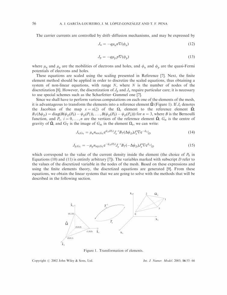
Since we shall have to perform various computations on each one of the elements of the mesh,it is advantageous to transform the elements into a reference element #OO (Figure 1). If Je denotesthe Jacobian of the map x ¼ xðxÞ of the Oe element to the reference element #OO;BT ðDcDÞ ¼ diagðBðcDðP0Þ cDðP1ÞÞ; . . . ;BðcDðP0Þ cDðPnÞÞÞ for n ¼ 3; where B is the Bernoullifunction, and Pi; i ¼ 0; . . . ; n are the vertices of the reference element #OO; Gm is the centre ofgravity of #OO; and GT is the image of Gm in the element Oe; we can write:

Jn;GT¼ mnnien;GT

ecDðP0ÞJte BT ðDcDÞJ

terefn jD ð14Þ

Jp;GT¼ mpniep;GT

ecDðP0ÞJte BT ðDcDÞJ

terefp jD ð15Þ

which correspond to the value of the current density inside the element (the choice of P0 inEquations (10) and (11) is entirely arbitrary [7]). The variables marked with subscript D refer tothe values of the discretized variable in the nodes of the mesh. Based on these expressions andusing the finite elements theory, the discretized equations are generated [9]. From theseequations, we obtain the linear systems that we are going to solve with the methods that will bedescribed in the following section.

x3^

3x

x2

x1

Ω e

0

1

3

2

-1Te

Te

(1,0,0)

(0,0,0)

(0,1,0)

(0,0,1)

^x1

^x2

Ω^

Figure 1. Transformation of elements.



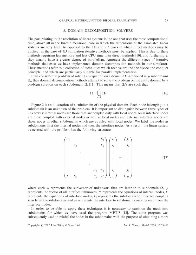
3. DOMAIN DECOMPOSITION SOLVERS

The part relating to the resolution of linear systems is the one that uses the most computationaltime, above all in the three-dimensional case in which the dimensions of the associated linearsystems are very high. As opposed to the 1D and 2D cases in which direct methods may beapplied, in the case of 3D simulation iterative methods must be applied. This is due to thesemethods requiring less memory and less CPU time than direct methods [10], and furthermore,they usually have a greater degree of parallelism. Amongst the different types of iterativemethods that exist we have implemented domain decomposition methods in our simulator.These methods refer to a collection of techniques which revolve around the divide and conquerprinciple, and which are particularly suitable for parallel implementation.

If we consider the problem of solving an equation on a domain O partitioned in p subdomainsOi; then domain decomposition methods attempt to solve the problem on the entire domain by aproblem solution on each subdomain Oi [11]. This means that Oi’s are such that

O ¼[pi¼1

Oi ð16Þ

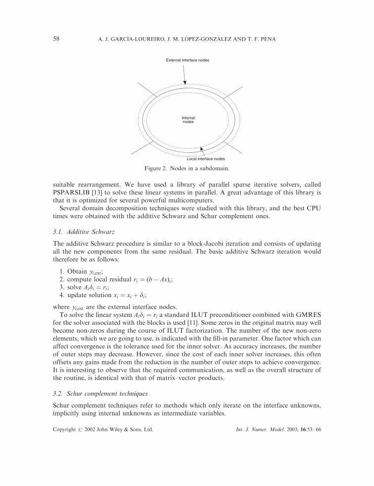
Figure 2 is an illustration of a subdomain of the physical domain. Each node belonging to asubdomain is an unknown of the problem. It is important to distinguish between three types ofunknowns: internal nodes are those that are coupled only with local nodes, local interface nodesare those coupled with external nodes as well as local nodes and external interface nodes arethose nodes in other subdomains which are coupled with local nodes. We label the nodes assubdomains, first the internal nodes and then the interface nodes. As a result, the linear systemassociated with the problem has the following structure:

B1 E1

B2 E2

:

:

:

Bp Ep

F1 F2 Fp C

0BBBBBBBBBBBBBB@

1CCCCCCCCCCCCCCA

x1

x2

:

:

:

xs

y

0BBBBBBBBBBBBBB@

1CCCCCCCCCCCCCCA

¼

f1

f2

:

:

:

fs

g

0BBBBBBBBBBBBBB@

1CCCCCCCCCCCCCCA

ð17Þ

where each xi represents the subvector of unknowns that are interior to subdomain Oi; yrepresents the vector of all interface unknowns, Bi represents the equations of internal nodes, Crepresents the equations of interface nodes, Ei represents the subdomain to interface couplingseen from the subdomains and Fi represents the interface to subdomain coupling seen from theinterface nodes.

In order to be able to apply these techniques it is necessary to partition the mesh intosubdomains for which we have used the program METIS [12]. The same program wassubsequently used to relabel the nodes in the subdomains with the purpose of obtaining a more



suitable rearrangement. We have used a library of parallel sparse iterative solvers, calledPSPARSLIB [13] to solve these linear systems in parallel. A great advantage of this library isthat it is optimized for several powerful multicomputers.

Several domain decomposition techniques were studied with this library, and the best CPUtimes were obtained with the additive Schwarz and Schur complement ones.

3.1. Additive Schwarz

The additive Schwarz procedure is similar to a block-Jacobi iteration and consists of updatingall the new components from the same residual. The basic additive Schwarz iteration wouldtherefore be as follows:

1. Obtain yi;ext;2. compute local residual ri ¼ ðb AxÞi;3. solve Aidi ¼ ri;4. update solution xi ¼ xi þ di;

where yi;ext are the external interface nodes.To solve the linear system Aidi ¼ ri a standard ILUT preconditioner combined with GMRES

for the solver associated with the blocks is used [11]. Some zeros in the original matrix may wellbecome non-zeros during the course of ILUT factorization. The number of the new non-zeroelements, which we are going to use, is indicated with the fill-in parameter. One factor which canaffect convergence is the tolerance used for the inner solver. As accuracy increases, the numberof outer steps may decrease. However, since the cost of each inner solver increases, this oftenoffsets any gains made from the reduction in the number of outer steps to achieve convergence.It is interesting to observe that the required communication, as well as the overall structure ofthe routine, is identical with that of matrix–vector products.

3.2. Schur complement techniques

Schur complement techniques refer to methods which only iterate on the interface unknowns,implicitly using internal unknowns as intermediate variables.

Internal nodes

External interface nodes

Local interface nodes

Figure 2. Nodes in a subdomain.



Consider the linear system (17) for the subdomain Oi described as

Bi Ei

Fi Ci

!xi

yi

!¼

fi

gi

!ð18Þ

in which Bi is assumed to be non-singular. From the first equation of (18) the unknown x can beexpressed as

xi ¼ B1i ðfi EiyiÞ ð19Þ

Upon substituting this into the second equation of (18), the following reduced system isobtained

ðCi FiB1i EiÞyi ¼ gi i FB1

i fi ð20Þ

Where the matrix Si ¼ Ci FiB1i Ei is called the Schur complement matrix associated with the

yi variable. If this system can be solved, all the interface variables y will become available, andthen the remaining unknowns can be computed using (19). Due to the particular structure of B;it should be observed that any linear system solution with it decouples into p separate systems.The parallelism in this situation arises from this natural decoupling.

4. RESULTS

Our simulator was developed for distributed-memory multicomputers using the multipleinstruction-multiple data strategy (MIMD) under the single program-multiple data paradigm(SPMD). It was implemented using the message passing interface (MPI) message passingstandard library [14]. The main advantage of using this library is that it is presently implementedin many computers, which guarantees the portability of the code.

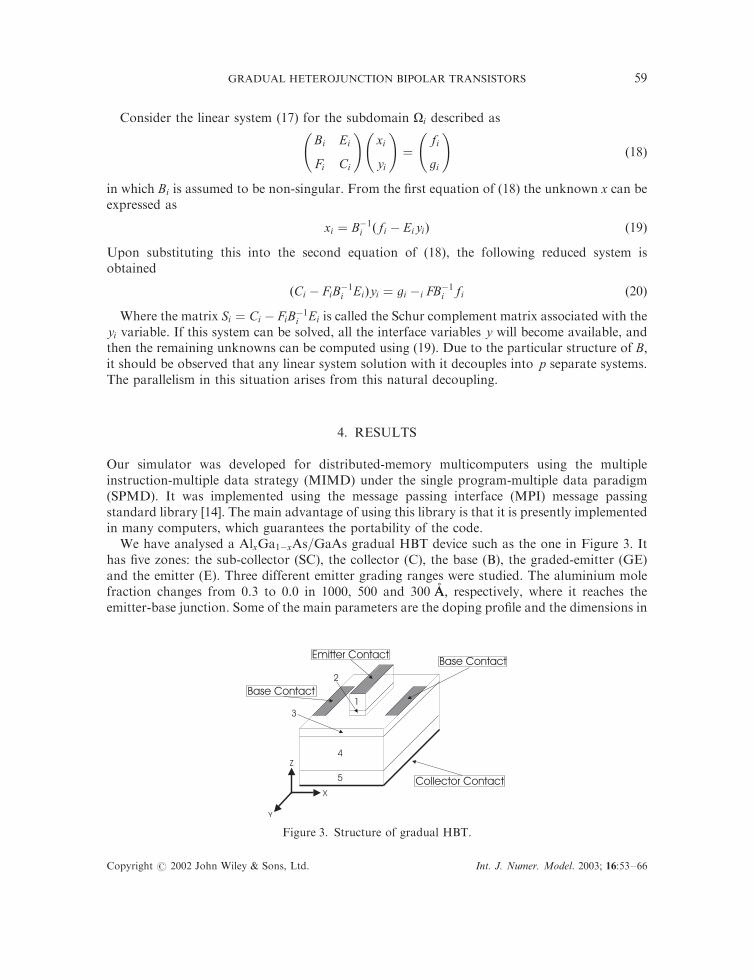
We have analysed a AlxGa1xAs=GaAs gradual HBT device such as the one in Figure 3. Ithas five zones: the sub-collector (SC), the collector (C), the base (B), the graded-emitter (GE)and the emitter (E). Three different emitter grading ranges were studied. The aluminium molefraction changes from 0.3 to 0.0 in 1000, 500 and 300 (AA; respectively, where it reaches theemitter-base junction. Some of the main parameters are the doping profile and the dimensions in

Figure 3. Structure of gradual HBT.



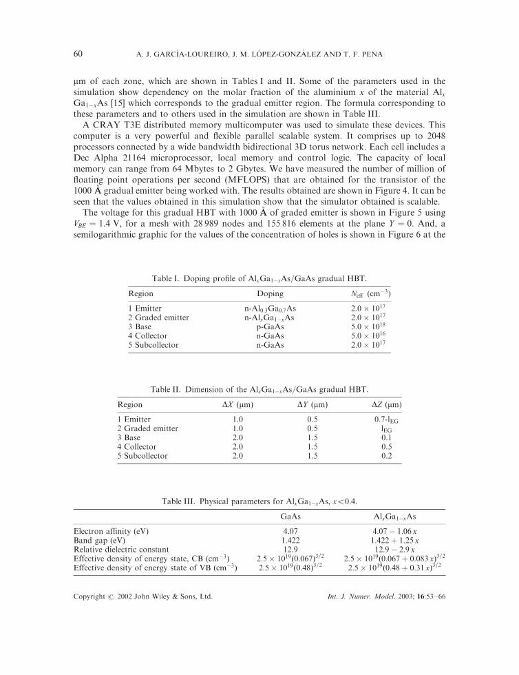
mm of each zone, which are shown in Tables I and II. Some of the parameters used in thesimulation show dependency on the molar fraction of the aluminium x of the material AlxGa1xAs [15] which corresponds to the gradual emitter region. The formula corresponding tothese parameters and to others used in the simulation are shown in Table III.

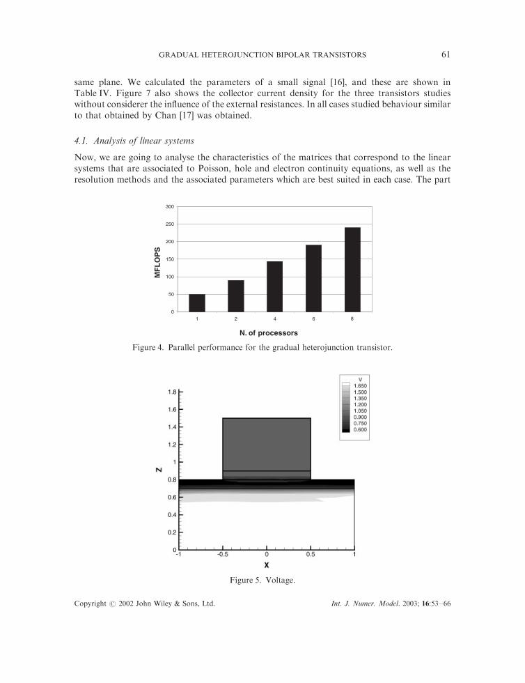
A CRAY T3E distributed memory multicomputer was used to simulate these devices. Thiscomputer is a very powerful and flexible parallel scalable system. It comprises up to 2048processors connected by a wide bandwidth bidirectional 3D torus network. Each cell includes aDec Alpha 21164 microprocessor, local memory and control logic. The capacity of localmemory can range from 64 Mbytes to 2 Gbytes. We have measured the number of million offloating point operations per second (MFLOPS) that are obtained for the transistor of the1000 (AA gradual emitter being worked with. The results obtained are shown in Figure 4. It can beseen that the values obtained in this simulation show that the simulator obtained is scalable.

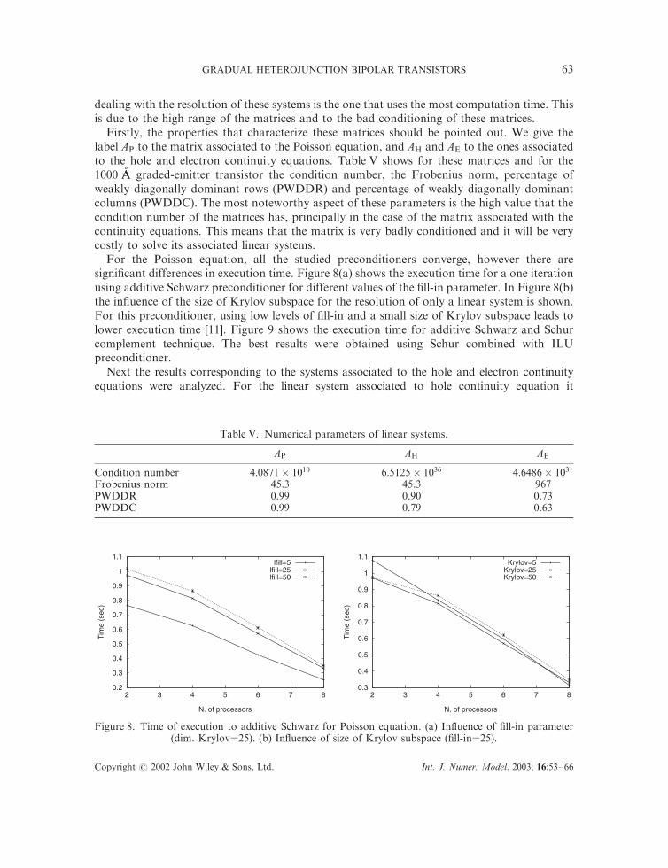
The voltage for this gradual HBT with 1000 (AA of graded emitter is shown in Figure 5 usingVBE ¼ 1:4 V; for a mesh with 28 989 nodes and 155 816 elements at the plane Y ¼ 0: And, asemilogarithmic graphic for the values of the concentration of holes is shown in Figure 6 at the

Table I. Doping profile of AlxGa1xAs=GaAs gradual HBT.

Region Doping Neff ðcm3Þ

1 Emitter n-Al0:3Ga0:7As 2:0 1017

2 Graded emitter n-AlxGa1xAs 2:0 1017

3 Base p-GaAs 5:0 1018

4 Collector n-GaAs 5:0 1016

5 Subcollector n-GaAs 2:0 1017

Table II. Dimension of the AlxGa1xAs=GaAs gradual HBT.

Region DX ðmmÞ DY ðmmÞ DZ ðmmÞ

1 Emitter 1.0 0.5 0.7-lEG2 Graded emitter 1.0 0.5 lEG3 Base 2.0 1.5 0.14 Collector 2.0 1.5 0.55 Subcollector 2.0 1.5 0.2

Table III. Physical parameters for AlxGa1xAs; x50:4:

GaAs AlxGa1xAs

Electron affinity (eV) 4.07 4:07 1:06 xBand gap (eV) 1.422 1:422þ 1:25 xRelative dielectric constant 12.9 12:9 2:9 xEffective density of energy state, CB ðcm3Þ 2:5 1019ð0:067Þ3=2 2:5 1019ð0:067þ 0:083 xÞ3=2

Effective density of energy state of VB ðcm3Þ 2:5 1019ð0:48Þ3=2 2:5 1019ð0:48þ 0:31 xÞ3=2



same plane. We calculated the parameters of a small signal [16], and these are shown inTable IV. Figure 7 also shows the collector current density for the three transistors studieswithout considerer the influence of the external resistances. In all cases studied behaviour similarto that obtained by Chan [17] was obtained.

4.1. Analysis of linear systems

Now, we are going to analyse the characteristics of the matrices that correspond to the linearsystems that are associated to Poisson, hole and electron continuity equations, as well as theresolution methods and the associated parameters which are best suited in each case. The part

0

50

100

150

200

250

300

1 2 4 6

N. of processors

MF

LO

PS

8

Figure 4. Parallel performance for the gradual heterojunction transistor.

Figure 5. Voltage.



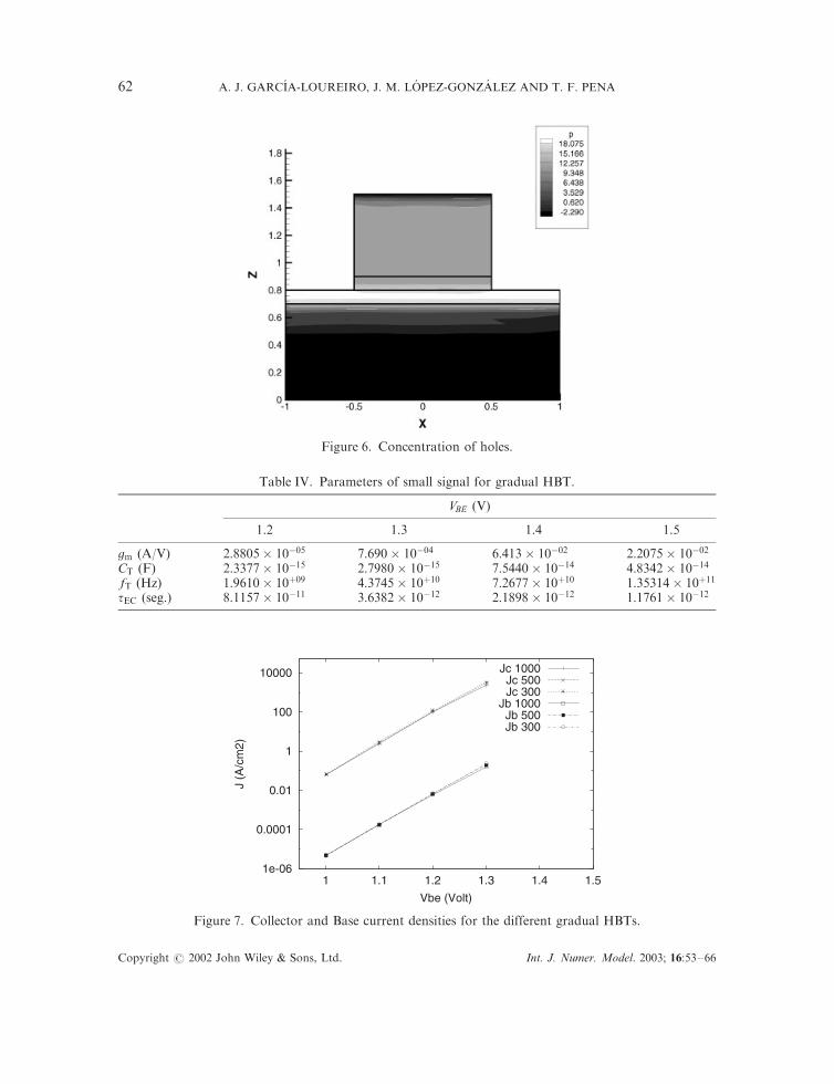
Figure 6. Concentration of holes.

1e-06

0.0001

0.01

1

100

10000

1 1.1 1.2 1.3 1.4 1.5

J (A

/cm

2)

Vbe (Volt)

Jc 1000Jc 500Jc 300

Jb 1000Jb 500Jb 300

Figure 7. Collector and Base current densities for the different gradual HBTs.

Table IV. Parameters of small signal for gradual HBT.

VBE (V)

1.2 1.3 1.4 1.5

gm (A/V) 2:8805 1005 7:690 1004 6:413 1002 2:2075 1002

CT (F) 2:3377 1015 2:7980 1015 7:5440 1014 4:8342 1014

fT (Hz) 1:9610 10þ09 4:3745 10þ10 7:2677 10þ10 1:35314 10þ11

tEC (seg.) 8:1157 1011 3:6382 1012 2:1898 1012 1:1761 1012



dealing with the resolution of these systems is the one that uses the most computation time. Thisis due to the high range of the matrices and to the bad conditioning of these matrices.

Firstly, the properties that characterize these matrices should be pointed out. We give thelabel AP to the matrix associated to the Poisson equation, and AH and AE to the ones associatedto the hole and electron continuity equations. Table V shows for these matrices and for the1000 (AA graded-emitter transistor the condition number, the Frobenius norm, percentage ofweakly diagonally dominant rows (PWDDR) and percentage of weakly diagonally dominantcolumns (PWDDC). The most noteworthy aspect of these parameters is the high value that thecondition number of the matrices has, principally in the case of the matrix associated with thecontinuity equations. This means that the matrix is very badly conditioned and it will be verycostly to solve its associated linear systems.

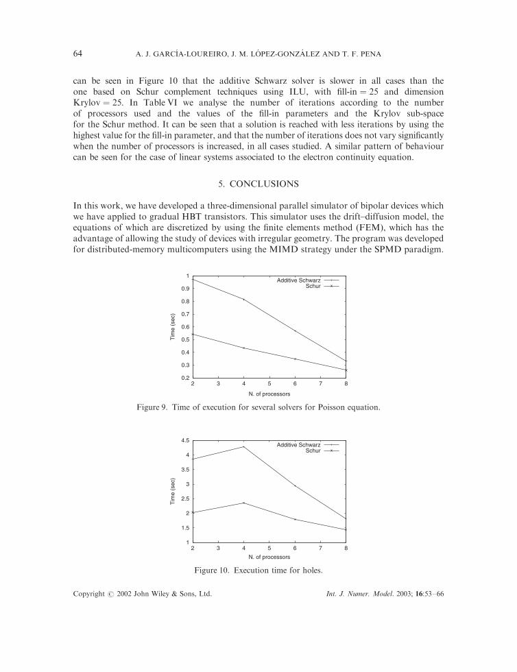
For the Poisson equation, all the studied preconditioners converge, however there aresignificant differences in execution time. Figure 8(a) shows the execution time for a one iterationusing additive Schwarz preconditioner for different values of the fill-in parameter. In Figure 8(b)the influence of the size of Krylov subspace for the resolution of only a linear system is shown.For this preconditioner, using low levels of fill-in and a small size of Krylov subspace leads tolower execution time [11]. Figure 9 shows the execution time for additive Schwarz and Schurcomplement technique. The best results were obtained using Schur combined with ILUpreconditioner.

Next the results corresponding to the systems associated to the hole and electron continuityequations were analyzed. For the linear system associated to hole continuity equation it

Table V. Numerical parameters of linear systems.

AP AH AE

Condition number 4:0871 1010 6:5125 1036 4:6486 1031

Frobenius norm 45.3 45.3 967PWDDR 0.99 0.90 0.73PWDDC 0.99 0.79 0.63

0.2

0.3

0.4

0.5

0.6

0.7

0.8

0.9

1

1.1

2 3 4 5 6 7 8

Tim

e (s

ec)

N. of processors

lfill=5lfill=25lfill=50

0.3

0.4

0.5

0.6

0.7

0.8

0.9

1

1.1

2 3 4 5 6 7 8

Tim

e (s

ec)

N. of processors

Krylov=5Krylov=25Krylov=50

Figure 8. Time of execution to additive Schwarz for Poisson equation. (a) Influence of fill-in parameter(dim. Krylov¼25). (b) Influence of size of Krylov subspace (fill-in¼25).



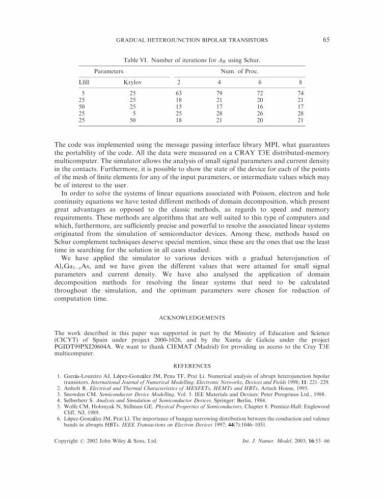
can be seen in Figure 10 that the additive Schwarz solver is slower in all cases than theone based on Schur complement techniques using ILU, with fill-in ¼ 25 and dimensionKrylov ¼ 25: In Table VI we analyse the number of iterations according to the numberof processors used and the values of the fill-in parameters and the Krylov sub-spacefor the Schur method. It can be seen that a solution is reached with less iterations by using thehighest value for the fill-in parameter, and that the number of iterations does not vary significantlywhen the number of processors is increased, in all cases studied. A similar pattern of behaviourcan be seen for the case of linear systems associated to the electron continuity equation.

5. CONCLUSIONS

In this work, we have developed a three-dimensional parallel simulator of bipolar devices whichwe have applied to gradual HBT transistors. This simulator uses the drift–diffusion model, theequations of which are discretized by using the finite elements method (FEM), which has theadvantage of allowing the study of devices with irregular geometry. The program was developedfor distributed-memory multicomputers using the MIMD strategy under the SPMD paradigm.

0.2

0.3

0.4

0.5

0.6

0.7

0.8

0.9

1

2 3 4 5 6 7 8

Tim

e (s

ec)

N. of processors

Additive SchwarzSchur

Figure 9. Time of execution for several solvers for Poisson equation.

1

1.5

2

2.5

3

3.5

4

4.5

2 3 4 5 6 7 8

Tim

e (s

ec)

N. of processors

Additive SchwarzSchur

Figure 10. Execution time for holes.



The code was implemented using the message passing interface library MPI, what guaranteesthe portability of the code. All the data were measured on a CRAY T3E distributed-memorymulticomputer. The simulator allows the analysis of small signal parameters and current densityin the contacts. Furthermore, it is possible to show the state of the device for each of the pointsof the mesh of finite elements for any of the input parameters, or intermediate values which maybe of interest to the user.

In order to solve the systems of linear equations associated with Poisson, electron and holecontinuity equations we have tested different methods of domain decomposition, which presentgreat advantages as opposed to the classic methods, as regards to speed and memoryrequirements. These methods are algorithms that are well suited to this type of computers andwhich, furthermore, are sufficiently precise and powerful to resolve the associated linear systemsoriginated from the simulation of semiconductor devices. Among these, methods based onSchur complement techniques deserve special mention, since these are the ones that use the leasttime in searching for the solution in all cases studied.

We have applied the simulator to various devices with a gradual heterojunction ofAlxGa1xAs; and we have given the different values that were attained for small signalparameters and current density. We have also analysed the application of domaindecomposition methods for resolving the linear systems that need to be calculatedthroughout the simulation, and the optimum parameters were chosen for reduction ofcomputation time.

ACKNOWLEDGEMENTS

The work described in this paper was supported in part by the Ministry of Education and Science(CICYT) of Spain under project 2000-1026, and by the Xunta de Galicia under the projectPGIDT99PXI20604A. We want to thank CIEMAT (Madrid) for providing us access to the Cray T3Emulticomputer.

REFERENCES

1. Garc!ııa-Loureiro AJ, L !oopez-Gonz!aalez JM, Pena TF, Prat Li. Numerical analysis of abrupt heterojunction bipolartransistors. International Journal of Numerical Modelling: Electronic Networks, Devices and Fields 1998; 11: 221–229.

2. Anholt R. Electrical and Thermal Characteristics of MESFETs, HEMTs and HBTs. Artech House, 1995.3. Snowden CM. Semiconductor Device Modelling. Vol. 5. IEE Materials and Devices: Peter Peregrinus Ltd., 1988.4. Selberherr S. Analysis and Simulation of Semiconductor Devices. Springer: Berlin, 1984.5. Wolfe CM, Holonyak N, Stillman GE. Physical Properties of Semiconductors, Chapter 8. Prentice-Hall: Englewood

Cliff, NJ, 1989.6. L !oopez-Gonz!aalez JM, Prat Ll. The importance of bangap narrowing distribution between the conduction and valence

bands in abrupts HBTs. IEEE Transactions on Electron Devices 1997; 44(7):1046–1051.

Table VI. Number of iterations for AH using Schur.

Parameters Num. of Proc.

Lfill Krylov 2 4 6 8

5 25 63 79 72 7425 25 18 21 20 2150 25 15 17 16 1725 5 25 28 26 2825 50 18 21 20 21



7. Markowich PA. The Stationary Semiconductor Device Equations. Springer: Berlin, 1986.8. Pena TF, Bruguera JD, Zapata EL. Finite element resolution of the 3D stationary semiconductor device equations

on multiprocessors. Journal of Integrated Computer-Aided Engineering 1997; 4(1):66–7.9. Becker EB, Carey GF, Oden JT. Finite Elements. Prentice-Hall: Englewood Cliffs, NJ, 1981.10. Heiser G, Pommerell C, Weis J, Fichner W. Three-dimensional numerical semiconductor device simulation:

algorithms, architectures, results. IEEE Transactions on Computer-Aided Design, 1991; 10(10):1218–1229.11. Saad Y. Iterative Methods for Sparse Linear Systems. PWS Publishing Co: New York, 1996.12. Karypis G, Kumar V. METIS: A software package for partitioning unstructured graphs, partitioning meshes, and

computing fill-reducing orderings of sparse matrices, University of Minnesota, 1997.13. Saad Y, Gen-Ching Lo, Kuznetsov S. PSPARSLIB users manual: a portable library of parallel sparse iterative

solvers. Technical Report, University of Minnesota, Department of Computer Science, 1997.14. MPI: A Message-Passing Interface Standard, http://www.mpi-forum.org, University of Tennessee, 1995.15. Adachi S. GaAs, AlAs and AlGaAs: material parameters for use in research and device applications. Journal of

Applied Physics 1985; 58(3):1–29.16. Stevan E. Laux. Techniques for small-signal analysis of semiconductor devices. IEEE Transactions on Electron

Devices 1985; 32(10):228–2037.17. Chan HC, Shieh TJ. A three-dimensional semiconductor device simulator for GaAs/AlGaAs heterojunction bipolar

transistor analysis. IEEE Transactions on Electron Devices 1991; 38(11):2427–2432.

AUTHORS’ BIOGRAPHIES

Antonio J. Garc!ııa-Loureiro received the MS degree in Physics from the University ofSantiago de Compostela in 1994 and the PhD degree from the University ofSantiago de Compostela in 1999. His doctoral research work was on modelling andsimulation of InP- and GaAs-based heterojunction bipolar transistors, havingdeveloped a numerical simulator about graded and abrupt HBTs, BIPS3D.Currently he is an assistance professor in the department of Electronics andComputer Science at the University of Santiago de Compotela. His research interestsinvolve HBTs for high-frequency, analytical and numerical simulation of bipolardevices.

Juan M. Lopez-Gonzalez received the BS and MSc degree in Physics from theUniversitat de Barcelona (UB) in 1987 and the PhD degree from the UniversitatPolitecnica de Catalunya (UPC), in Barcelona, Spain, in 1994. His doctoral researchwork was on modelling and simulation of InP-, Si- and GaAs-based heterojunctionbipolar transistors, having developed a numerical simulator about graded andabrupt HBTs, HBTSIM.He is an Associate Professor in the Departament dEnginyeria Electronica at theUPC, Spain. During 1991 and 1992 was a Visitor at University of California SanDiego, Department of Electrical and Computer Engineering. His research interestsinclude HBTs for high-frequency, high-power and/or high velocity applications,

analytical and numerical simulation of bipolar devices, III–V semiconductor compounds and their materialparametrization.

Tom!aas F. Pena received the MS degree in Physics from the University of Santiago deCompostela in 1989 and the PhD degree from the University of Santiago deCompostela in 1994. Currently he is a associate professor in the department ofElectronics and Computer Science at the University of Santiago de Compostela. Hisresearch interests involve parallel numerical algorithms for dense and sparsematrices, data parallel programming for irregular algorithms, FEM for modellingand simulation of homotransistors and heterojunction bipolar transistors, parallelBEM methods, and parallel volume rendering for computer graphics.



Documents

A parallel 3D semiconductor device simulator for gradual heterojunction bipolar transistors