ANSWERING CONJUNCTIVE QUERIES WITH INEQUALITIES

Paris Koutris1

Tova Milo2

Sudeepa Roy1

Dan Suciu1 ICDT 2015

1 University of Washington2 Tel Aviv University

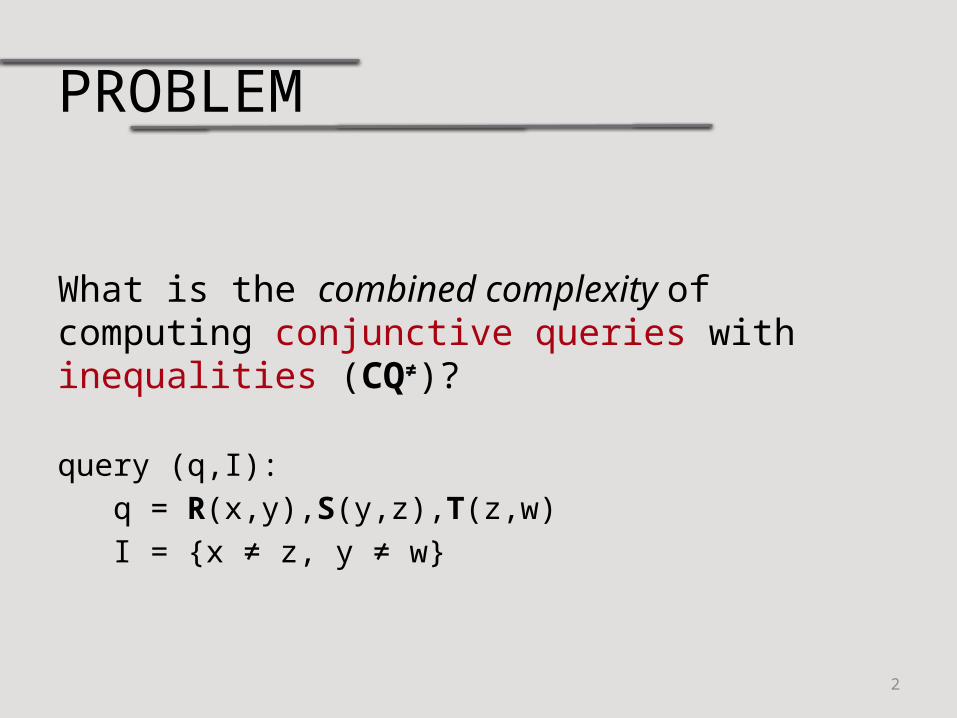
PROBLEM

What is the combined complexity of computing conjunctive queries with inequalities (CQ≠)?

query (q,I): q = R(x,y),S(y,z),T(z,w) I = {x ≠ z, y ≠ w}

2

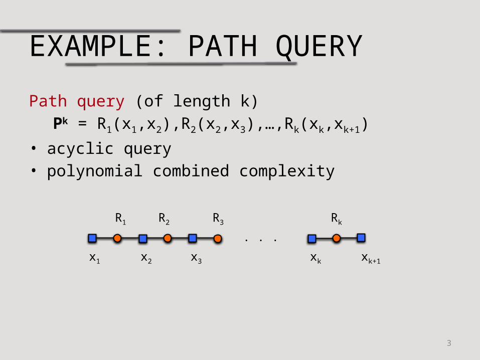
EXAMPLE: PATH QUERY

Path query (of length k)Pk = R1(x1,x2),R2(x2,x3),…,Rk(xk,xk+1)

• acyclic query• polynomial combined complexity

3

x1 x2 x3

. . .

xk xk+1

R1 R2 R3 Rk

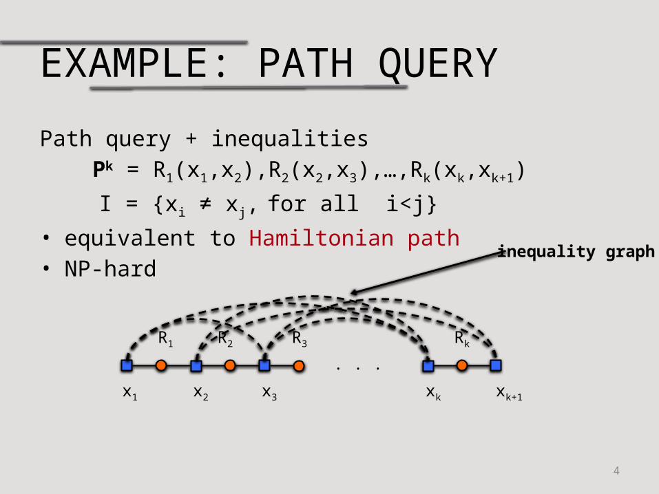
EXAMPLE: PATH QUERY

Path query + inequalities Pk = R1(x1,x2),R2(x2,x3),…,Rk(xk,xk+1)

I = {xi ≠ xj, for all i<j}

• equivalent to Hamiltonian path• NP-hard

4

x1 x2 x3

. . .

xk xk+1

R1 R2 R3 Rk

inequality graph

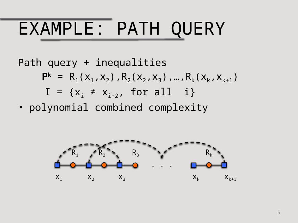
EXAMPLE: PATH QUERY

Path query + inequalities Pk = R1(x1,x2),R2(x2,x3),…,Rk(xk,xk+1)

I = {xi ≠ xi+2, for all i}

• polynomial combined complexity

5

x1 x2 x3

. . .

xk xk+1

R1 R2 R3 Rk

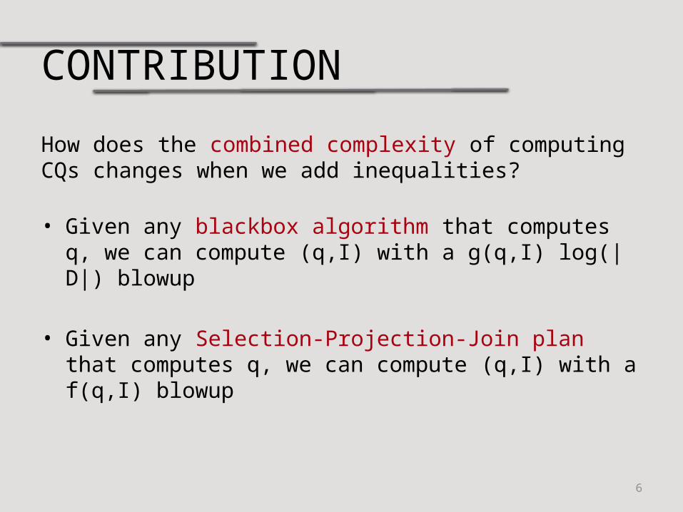
CONTRIBUTION

How does the combined complexity of computing CQs changes when we add inequalities?

• Given any blackbox algorithm that computes q, we can compute (q,I) with a g(q,I) log(|D|) blowup

• Given any Selection-Projection-Join plan that computes q, we can compute (q,I) with a f(q,I) blowup

6

OUTLINE

7

Color Coding

The Main Technique

Query Plans for Inequalities

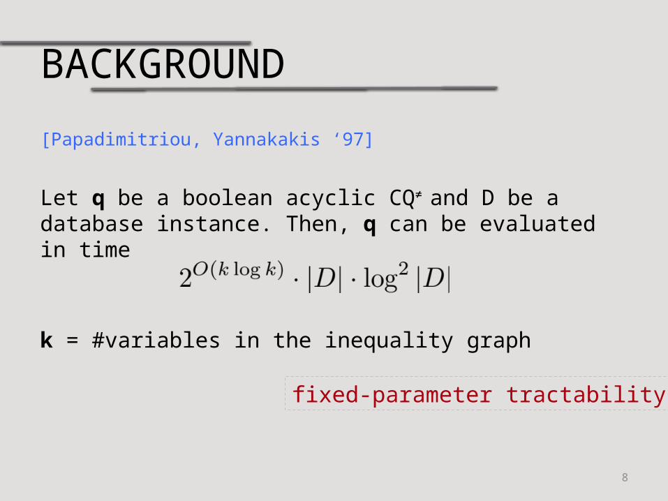
BACKGROUND

[Papadimitriou, Yannakakis ‘97]

Let q be a boolean acyclic CQ≠ and D be a database instance. Then, q can be evaluated in time

k = #variables in the inequality graph

8

fixed-parameter tractability

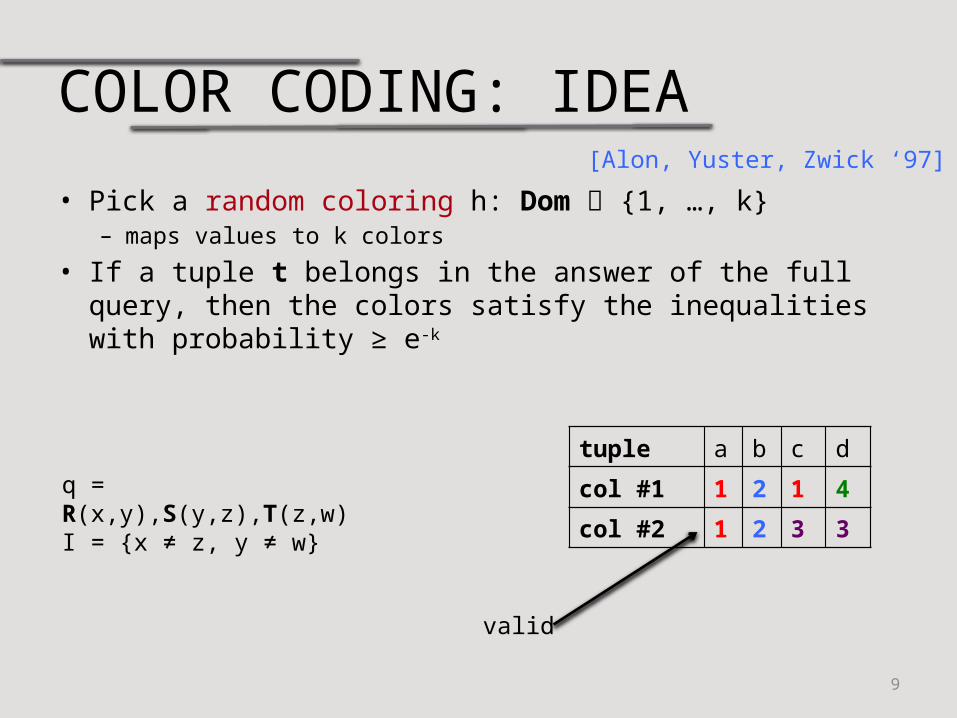
COLOR CODING: IDEA

• Pick a random coloring h: Dom {1, …, k}– maps values to k colors

• If a tuple t belongs in the answer of the full query, then the colors satisfy the inequalities with probability ≥ e-k

9

q = R(x,y),S(y,z),T(z,w)I = {x ≠ z, y ≠ w}

tuple a b c d

col #1 1 2 1 4

col #2 1 2 3 3

valid

[Alon, Yuster, Zwick ‘97]

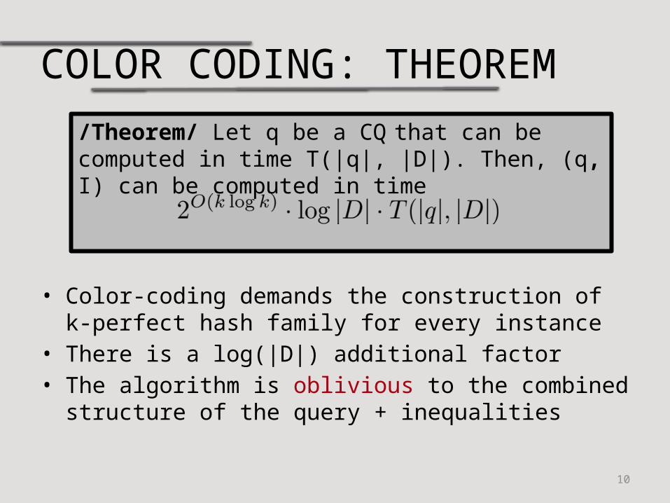
COLOR CODING: THEOREM

/Theorem/ Let q be a CQ that can be computed in time T(|q|, |D|). Then, (q, I) can be computed in time

10

• Color-coding demands the construction of k-perfect hash family for every instance

• There is a log(|D|) additional factor• The algorithm is oblivious to the combined structure of the

query + inequalities

OUTLINE

11

Color Coding

The Main Technique

Query Plans for Inequalities

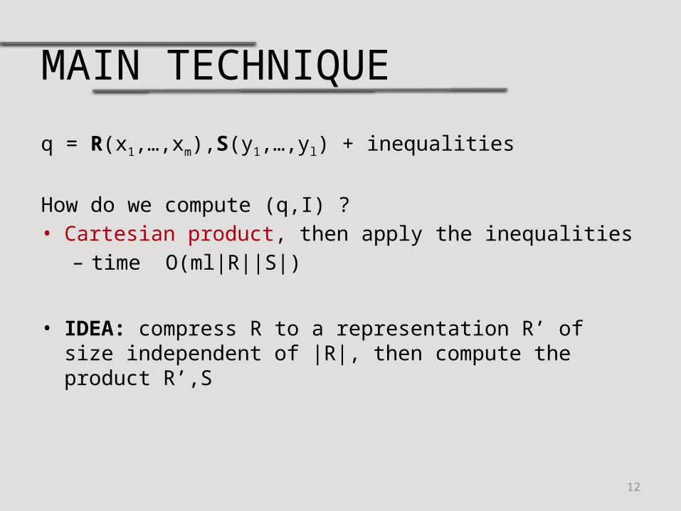
MAIN TECHNIQUE

q = R(x1,…,xm),S(y1,…,yl) + inequalities

How do we compute (q,I) ?• Cartesian product, then apply the inequalities– time O(ml|R||S|)

• IDEA: compress R to a representation R’ of size independent of |R|, then compute the product R’,S

12

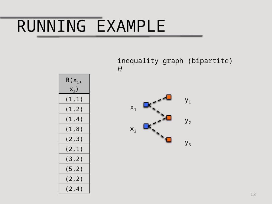
RUNNING EXAMPLE

inequality graph (bipartite) H

13

x1

x2

y1

y2

y3

R(x1, x2)

(1,1)

(1,2)

(1,4)

(1,8)

(2,3)

(2,1)

(3,2)

(5,2)

(2,2)

(2,4)

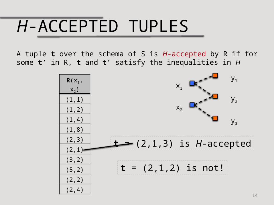
H-ACCEPTED TUPLES

14

A tuple t over the schema of S is H-accepted by R if for some t’ in R, t and t’ satisfy the inequalities in H

t = (2,1,3) is H-accepted

t = (2,1,2) is not!

R(x1, x2)

(1,1)

(1,2)

(1,4)

(1,8)

(2,3)

(2,1)

(3,2)

(5,2)

(2,2)

(2,4)

x1

x2

y1

y2

y3

H-EQUIVALENCE

15

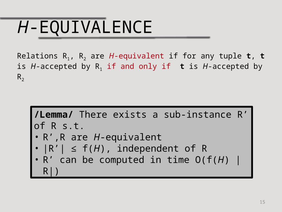
Relations R1, R2 are H-equivalent if for any tuple t, t is H-accepted by R1 if and only if t is H-accepted by R2

/Lemma/ There exists a sub-instance R’ of R s.t.• R’,R are H-equivalent • |R’| ≤ f(H), independent of R• R’ can be computed in time O(f(H) |R|)

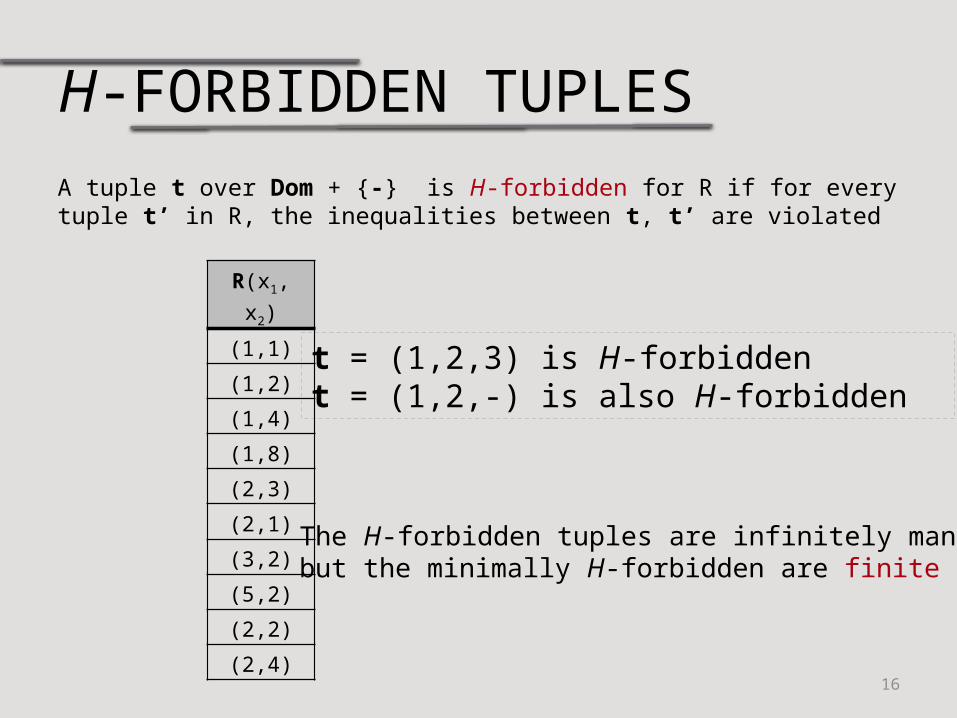
H-FORBIDDEN TUPLES

16

A tuple t over Dom + {-} is H-forbidden for R if for every tuple t’ in R, the inequalities between t, t’ are violated

t = (1,2,3) is H-forbidden t = (1,2,-) is also H-forbidden

The H-forbidden tuples are infinitely manybut the minimally H-forbidden are finite

R(x1, x2)

(1,1)

(1,2)

(1,4)

(1,8)

(2,3)

(2,1)

(3,2)

(5,2)

(2,2)

(2,4)

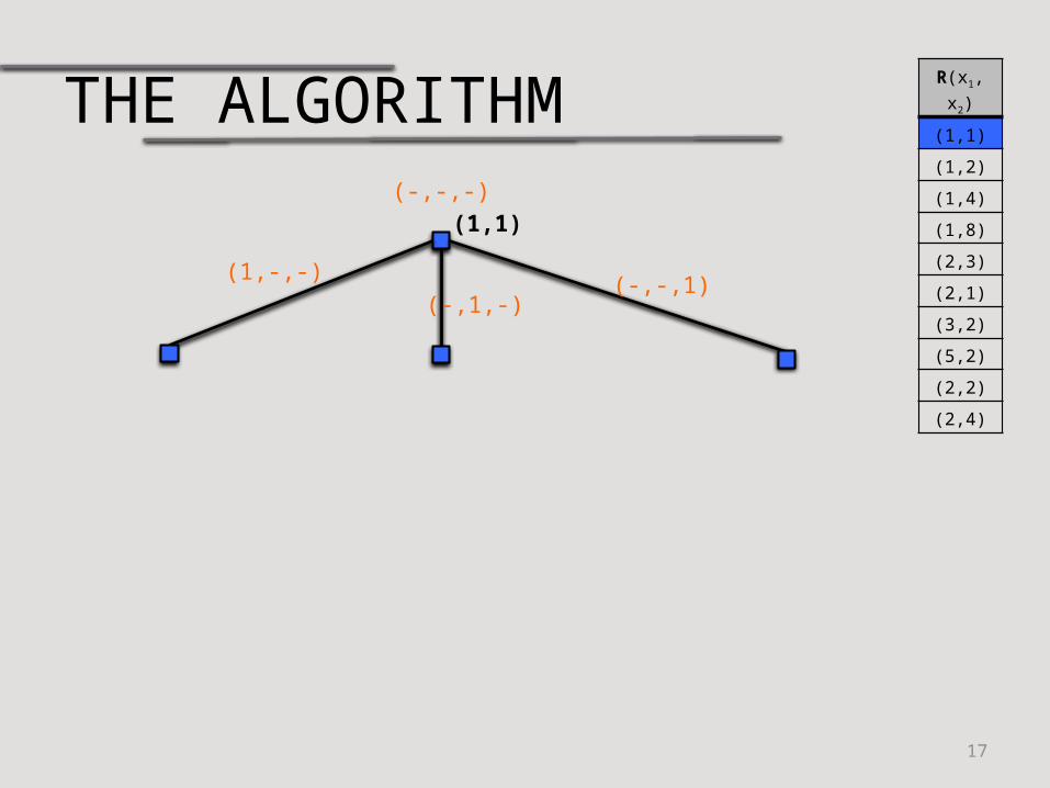
THE ALGORITHM

17

(1,1)(-,-,-)

(1,-,-)(-,1,-)

(-,-,1)

R(x1, x2)

(1,1)

(1,2)

(1,4)

(1,8)

(2,3)

(2,1)

(3,2)

(5,2)

(2,2)

(2,4)

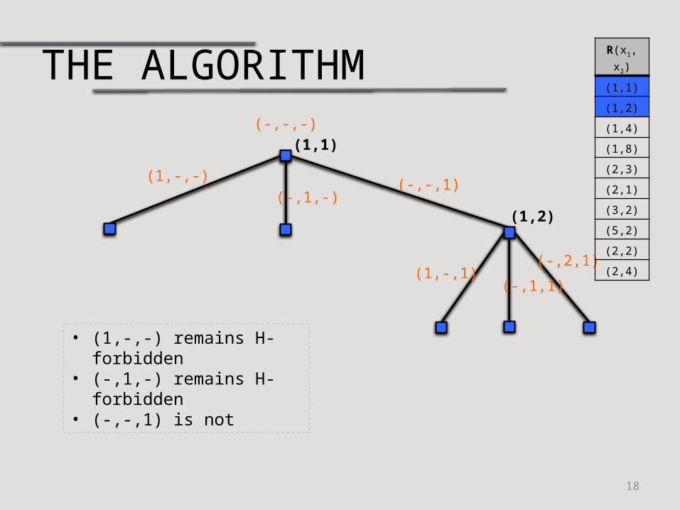
THE ALGORITHM

18

(1,1)(-,-,-)

(1,-,-)(-,1,-)

(-,-,1)

(1,2)

(-,2,1)

(-,1,1)(1,-,1)

R(x1, x2)

(1,1)

(1,2)

(1,4)

(1,8)

(2,3)

(2,1)

(3,2)

(5,2)

(2,2)

(2,4)

• (1,-,-) remains H-forbidden• (-,1,-) remains H-forbidden• (-,-,1) is not

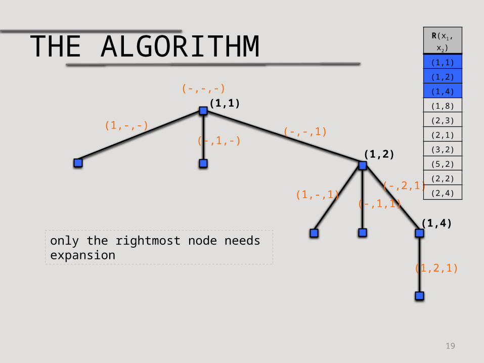
THE ALGORITHM

19

(1,1)(-,-,-)

(1,-,-)(-,1,-)

(-,-,1)

(1,2)

(-,2,1)

(-,1,1)(1,-,1)

(1,4)

(1,2,1)

R(x1, x2)

(1,1)

(1,2)

(1,4)

(1,8)

(2,3)

(2,1)

(3,2)

(5,2)

(2,2)

(2,4)

only the rightmost node needs expansion

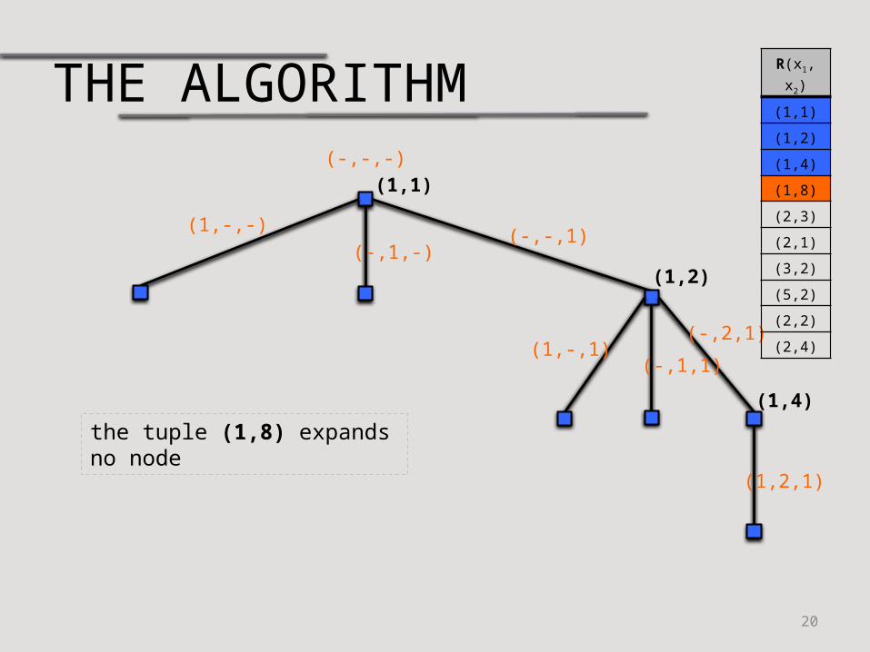
THE ALGORITHM

20

(1,1)(-,-,-)

(1,-,-)(-,1,-)

(-,-,1)

(1,2)

(-,2,1)

(-,1,1)(1,-,1)

(1,4)

(1,2,1)

R(x1, x2)

(1,1)

(1,2)

(1,4)

(1,8)

(2,3)

(2,1)

(3,2)

(5,2)

(2,2)

(2,4)

the tuple (1,8) expands no node

THE ALGORITHM

21

(1,1)(-,-,-)

(1,-,-)(-,1,-)

(-,-,1)

(1,2)

(-,2,1)

(-,1,1)(1,-,1)

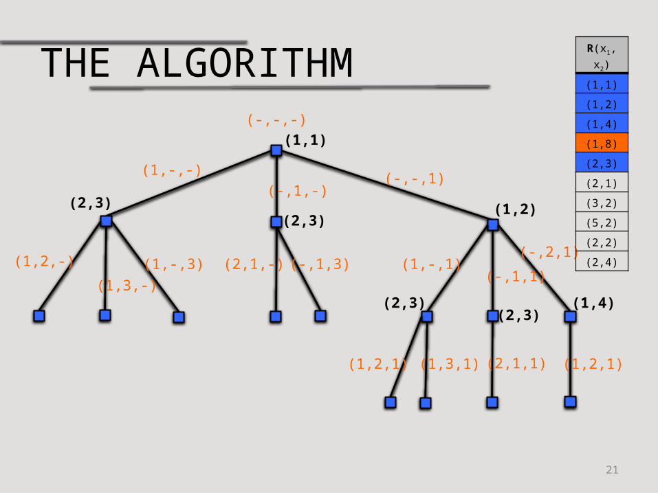
(2,3)(2,3)

(2,3)(2,3)

(2,1,1)

(1,2,-)

(1,3,-)

(1,-,3) (2,1,-) (-,1,3)

(1,2,1) (1,3,1)

(1,4)

(1,2,1)

R(x1, x2)

(1,1)

(1,2)

(1,4)

(1,8)

(2,3)

(2,1)

(3,2)

(5,2)

(2,2)

(2,4)

THE ALGORITHM

22

(1,1)(-,-,-)

(1,-,-)(-,1,-)

(-,-,1)

(1,2)

(-,2,1)

(-,1,1)(1,-,1)

(2,3)(2,3)

(2,3)(2,3)

(2,1,1)

(1,2,-)

(1,3,-)

(1,-,3) (2,1,-) (-,1,3)

(1,2,1) (1,3,1)

(1,4)

(1,2,1)

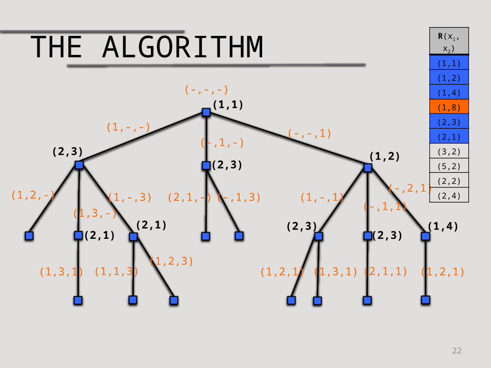
(2,1)(2,1)

(1,3,1) (1,1,3)(1,2,3)

R(x1, x2)

(1,1)

(1,2)

(1,4)

(1,8)

(2,3)

(2,1)

(3,2)

(5,2)

(2,2)

(2,4)

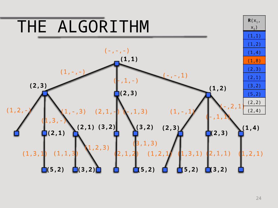
THE ALGORITHM

23

(1,1)(-,-,-)

(1,-,-)(-,1,-)

(-,-,1)

(1,2)

(-,2,1)

(-,1,1)(1,-,1)

(2,3)(2,3)

(2,3)(2,3)

(2,1,1)

(1,2,-)

(1,3,-)

(1,-,3) (2,1,-) (-,1,3)

(1,2,1) (1,3,1)

(1,4)

(1,2,1)

(2,1)(2,1)

(1,3,1) (1,1,3)(1,2,3)

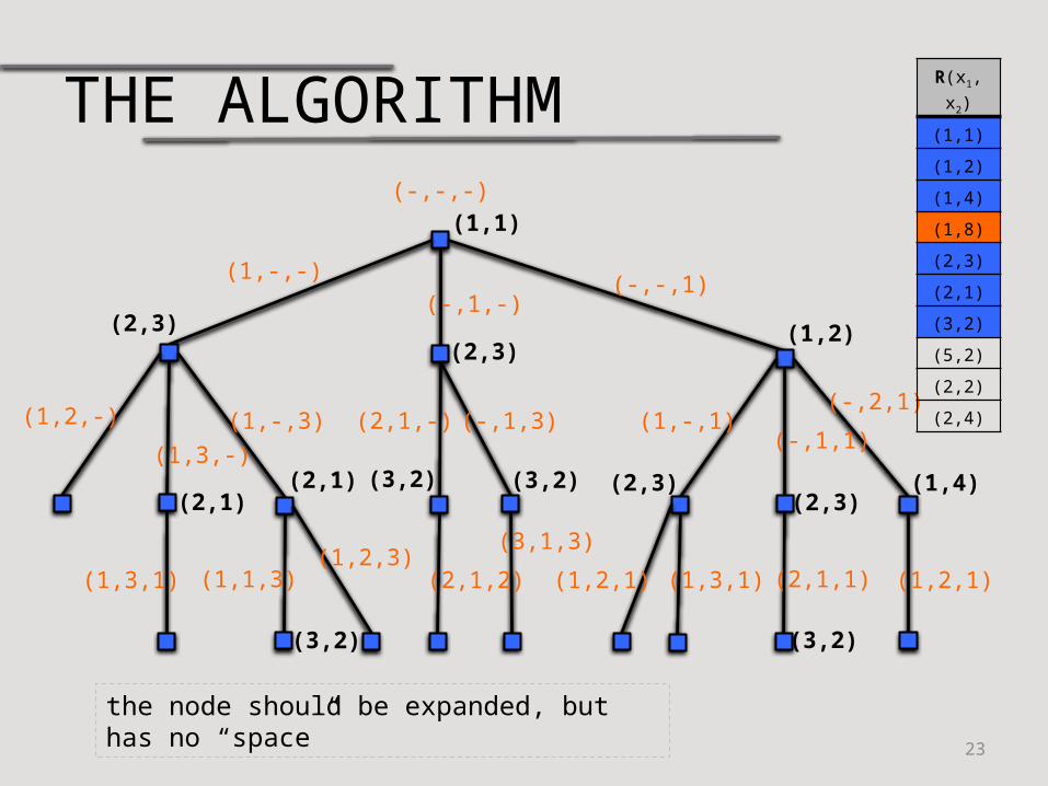
(3,2)

(3,2) (3,2)

(2,1,2)

(3,1,3)

(3,2)

R(x1, x2)

(1,1)

(1,2)

(1,4)

(1,8)

(2,3)

(2,1)

(3,2)

(5,2)

(2,2)

(2,4)

the node should be expanded, but has no “space”

THE ALGORITHM

24

(1,1)(-,-,-)

(1,-,-)(-,1,-)

(-,-,1)

(1,2)

(-,2,1)

(-,1,1)(1,-,1)

(2,3)(2,3)

(2,3)(2,3)

(2,1,1)

(1,2,-)

(1,3,-)

(1,-,3) (2,1,-) (-,1,3)

(1,2,1) (1,3,1)

(1,4)

(1,2,1)

(2,1)(2,1)

(1,3,1) (1,1,3)(1,2,3)

(3,2)

(3,2) (3,2)

(2,1,2)

(3,1,3)

(3,2)(5,2) (5,2) (5,2)

R(x1, x2)

(1,1)

(1,2)

(1,4)

(1,8)

(2,3)

(2,1)

(3,2)

(5,2)

(2,2)

(2,4)

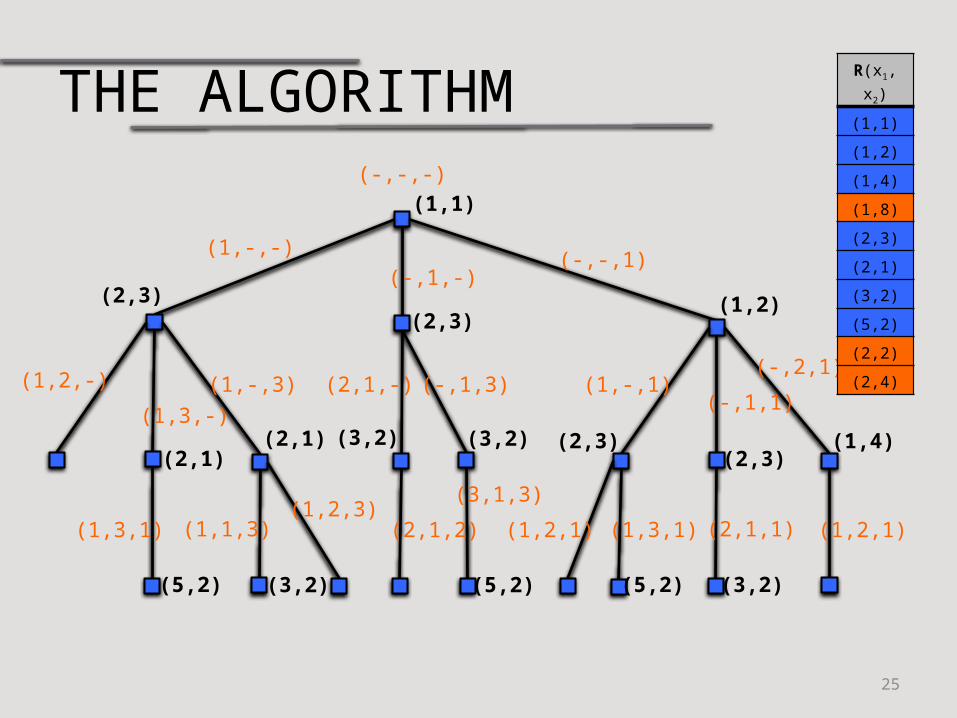
THE ALGORITHM

25

(1,1)(-,-,-)

(1,-,-)(-,1,-)

(-,-,1)

(1,2)

(-,2,1)

(-,1,1)(1,-,1)

(2,3)(2,3)

(2,3)(2,3)

(2,1,1)

(1,2,-)

(1,3,-)

(1,-,3) (2,1,-) (-,1,3)

(1,2,1) (1,3,1)

(1,4)

(1,2,1)

(2,1)(2,1)

(1,3,1) (1,1,3)(1,2,3)

(3,2)

(3,2) (3,2)

(2,1,2)

(3,1,3)

(3,2)(5,2) (5,2) (5,2)

R(x1, x2)

(1,1)

(1,2)

(1,4)

(1,8)

(2,3)

(2,1)

(3,2)

(5,2)

(2,2)

(2,4)

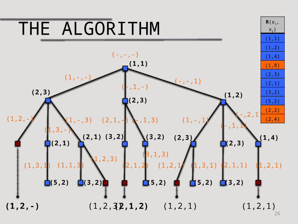
THE ALGORITHM

26

(1,1)(-,-,-)

(1,-,-)(-,1,-)

(-,-,1)

(1,2)

(-,2,1)

(-,1,1)(1,-,1)

(2,3)(2,3)

(2,3)(2,3)

(2,1,1)

(1,2,-)

(1,3,-)

(1,-,3) (2,1,-) (-,1,3)

(1,2,1) (1,3,1)

(1,4)

(1,2,1)

(2,1)(2,1)

(1,3,1) (1,1,3)(1,2,3)

(3,2)

(3,2) (3,2)

(2,1,2)

(3,1,3)

(3,2)(5,2) (5,2) (5,2)

R(x1, x2)

(1,1)

(1,2)

(1,4)

(1,8)

(2,3)

(2,1)

(3,2)

(5,2)

(2,2)

(2,4)

(1,2,-) (1,2,3) (2,1,2) (1,2,1) (1,2,1)

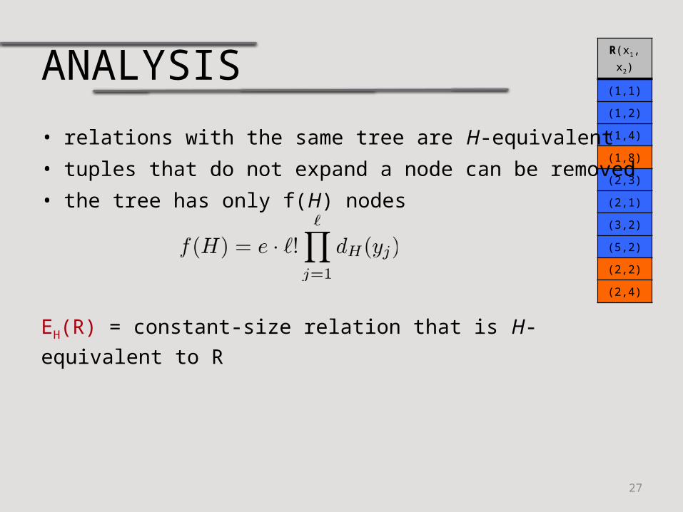
ANALYSIS

27

R(x1, x2)

(1,1)

(1,2)

(1,4)

(1,8)

(2,3)

(2,1)

(3,2)

(5,2)

(2,2)

(2,4)

• relations with the same tree are H-equivalent• tuples that do not expand a node can be removed• the tree has only f(H) nodes

EH(R) = constant-size relation that is H-equivalent to R

OUTLINE

28

Color Coding

The Main Technique

Query Plans for Inequalities

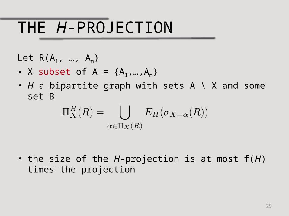
THE H-PROJECTION

29

Let R(A1, …, Am)

• X subset of A = {A1,…,Am}

• H a bipartite graph with sets A \ X and some set B

• the size of the H-projection is at most f(H) times the projection

SPJ PLANS

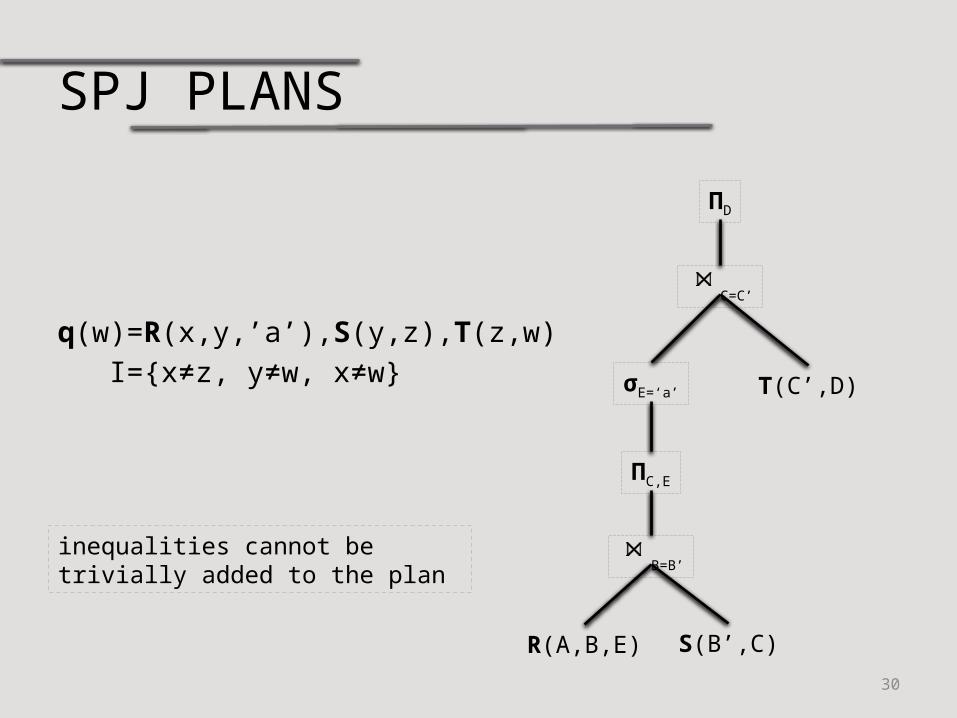
30

q(w)=R(x,y,’a’),S(y,z),T(z,w) I={x≠z, y≠w, x≠w}

R(A,B,E) S(B’,C)

ΠC,E

σE=‘a’

ΠD

T(C’,D)

B=B’

C=C’

inequalities cannot be trivially added to the plan

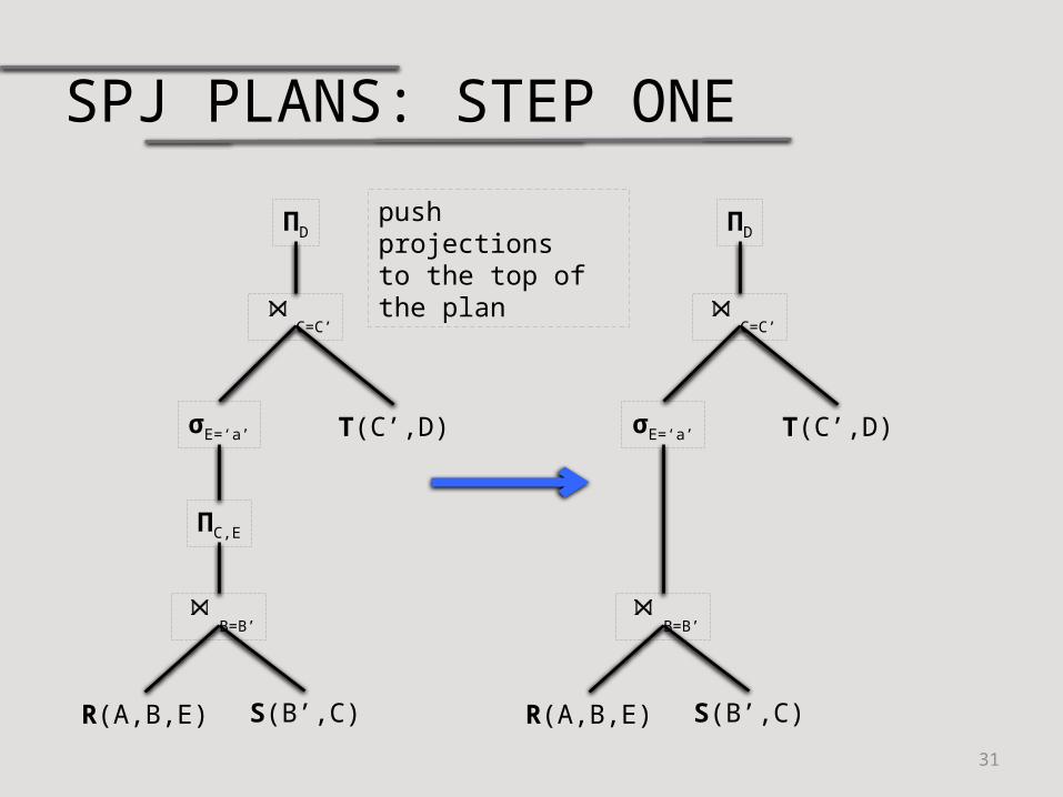
SPJ PLANS: STEP ONE

31

R(A,B,E) S(B’,C)

ΠC,E

σE=‘a’

ΠD

T(C’,D)

B=B’

C=C’

R(A,B,E) S(B’,C)

σE=‘a’

ΠD

T(C’,D)

B=B’

C=C’

push projectionsto the top of the plan

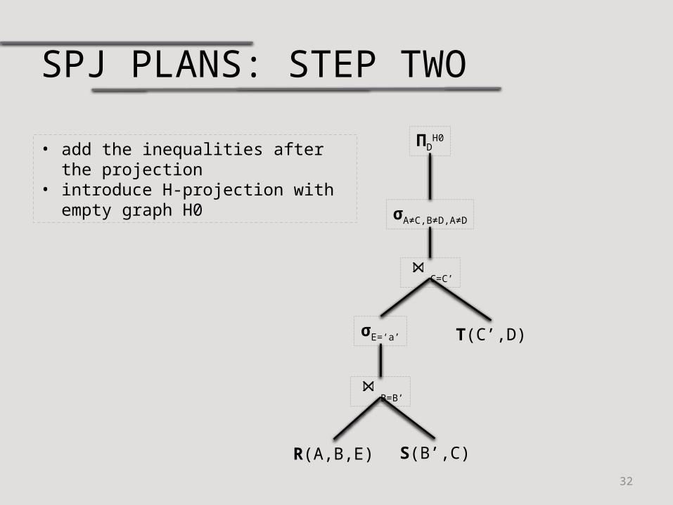
SPJ PLANS: STEP TWO

32

R(A,B,E) S(B’,C)

σE=‘a’

ΠDH0

T(C’,D)

B=B’

C=C’

• add the inequalities after the projection• introduce H-projection with empty

graph H0σA≠C,B≠D,A≠D

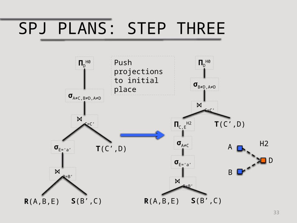
SPJ PLANS: STEP THREE

33

R(A,B,E) S(B’,C)

σE=‘a’

ΠDH0

T(C’,D)

B=B’

C=C’

Push projections to initial place

σA≠C,B≠D,A≠D

R(A,B,E) S(B’,C)

σE=‘a’

ΠDH0

T(C’,D)

B=B’

C=C’

σB≠D,A≠D

ΠC,EH2

σA≠C A

B

D

H2

SPJ PLANS: STEP THREE

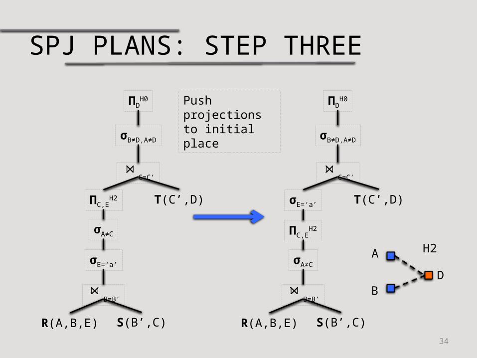
34

Push projections to initial place

R(A,B,E) S(B’,C)

σE=‘a’

ΠDH0

T(C’,D)

B=B’

C=C’

σB≠D,A≠D

ΠC,EH2

σA≠C

A

BD

H2

R(A,B,E) S(B’,C)

σE=‘a’

ΠDH0

T(C’,D)

B=B’

C=C’

σB≠D,A≠D

ΠC,EH2

σA≠C

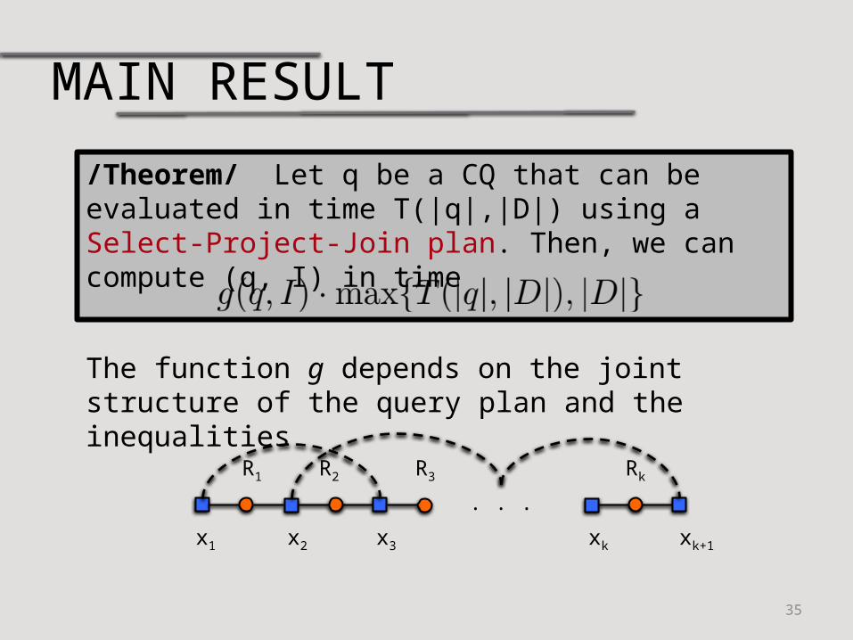
MAIN RESULT

/Theorem/ Let q be a CQ that can be evaluated in time T(|q|,|D|) using a Select-Project-Join plan. Then, we can compute (q, I) in time

35

x1 x2 x3

. . .

xk xk+1

R1 R2 R3 Rk

The function g depends on the joint structure of the query plan and the inequalities

CONCLUSION

36

What is the complexity of computing CQ≠ ?• color-coding for any CQ≠

• SPJ query plans with inequalities• In the paper : analysis of other structural properties

Open questions• can we apply the technique to arbitrary join algorithms?• other classes of queries: UCQs, Datalog

Thank you!

37

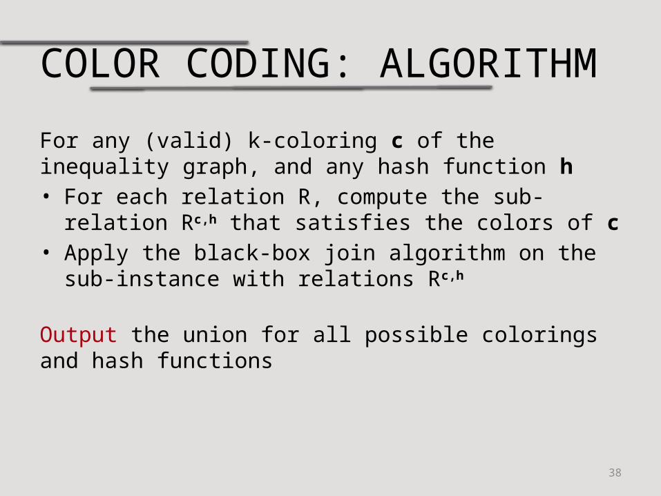
COLOR CODING: ALGORITHM

For any (valid) k-coloring c of the inequality graph, and any hash function h• For each relation R, compute the sub-relation Rc,h that

satisfies the colors of c• Apply the black-box join algorithm on the sub-instance

with relations Rc,h

Output the union for all possible colorings and hash functions

38