Embed Size (px)
Citation preview

c©Copyright 2015
Paraschos Koutris
Query Processing for Massively Parallel Systems
Paraschos Koutris
A dissertationsubmitted in partial fulfillment of the
requirements for the degree of
Doctor of Philosophy
University of Washington
2015
Reading Committee:
Dan Suciu, Chair
Paul Beame
Magdalena Balazinska
Program Authorized to Offer Degree:Computer Science and Engineering

University of Washington
Abstract
Query Processing for Massively Parallel Systems
Paraschos Koutris
Chair of the Supervisory Committee:Professor Dan Suciu
Computer Science and Engineering
The need to analyze and understand big data has changed the landscape of data manage-
ment over the last years. To process the large amounts of data available to users in both
industry and science, many modern data management systems leverage the power of massive
parallelism. The challenge of scaling computation to thousands of processing units demands
that we change our thinking on how we design such systems, and on how we analyze and
design parallel algorithms. In this dissertation, I study the fundamental problem of query
processing for modern massively parallel architectures.
I propose a theoretical model, the MPC model (Massively Parallel Computation), to
analyze the performance of parallel algorithms for query processing. In the MPC model, the
data is initially evenly distributed among p servers. The computation proceeds in rounds:
each round consists of some local computation followed by global exchange of data between
the servers. The computational complexity of an algorithm is characterized by both the
number of rounds necessary, and the maximum amount of data, or maximum load, that each
processor receives. The challenge is to identify the optimal tradeoff between the number of
rounds and maximum load for various computational tasks.
As a first step towards understanding query processing in the MPC model, we study
conjunctive queries (multiway joins) for a single round. We show that a particular type of
distributed algorithm, the HyperCube algorithm, can optimally compute join queries when
restricted to one communication round and data without skew.
In most real-world applications, data has skew (for example a graph with nodes of large
degree) that causes an uneven distribution of the load, and thus reduces the effectiveness
of parallelism. We show that the HyperCube algorithm is more resilient to skew than
traditional parallel query plans. To deal with any case of skew, we also design data-sensitive
techniques that identify the outliers in the data and alleviate the effect of skew by further
splitting the computation to more servers.
In the case of multiple rounds, we present nearly optimal algorithms for conjunctive
queries for the case of data without skew. A surprising consequence of our results is that
they can be applied to analyze iterative computational tasks: we can prove that, in order to
compute the connected components of a graph, any algorithm requires more than a constant
number of communication rounds. Finally, we show a surprising connection of the MPC
model with algorithms in the external memory model of computation.
TABLE OF CONTENTS
Page
List of Figures . . . . . . . . . . . . . . . . . . . . . . . . . . . . . . . . . . . . . . . iii
List of Tables . . . . . . . . . . . . . . . . . . . . . . . . . . . . . . . . . . . . . . . . iv
Chapter 1: Introduction . . . . . . . . . . . . . . . . . . . . . . . . . . . . . . . . 1
1.1 Motivation . . . . . . . . . . . . . . . . . . . . . . . . . . . . . . . . . . . . . 1
1.2 Contribution . . . . . . . . . . . . . . . . . . . . . . . . . . . . . . . . . . . . 4
1.3 Organization . . . . . . . . . . . . . . . . . . . . . . . . . . . . . . . . . . . 7
Chapter 2: Background . . . . . . . . . . . . . . . . . . . . . . . . . . . . . . . . . 8
2.1 Conjunctive Queries . . . . . . . . . . . . . . . . . . . . . . . . . . . . . . . 8
2.2 Entropy . . . . . . . . . . . . . . . . . . . . . . . . . . . . . . . . . . . . . . 14
2.3 Yao’s Principle . . . . . . . . . . . . . . . . . . . . . . . . . . . . . . . . . . 15
2.4 Friedgut’s Inequality . . . . . . . . . . . . . . . . . . . . . . . . . . . . . . . 15
Chapter 3: The Massively Parallel Computation Model . . . . . . . . . . . . . . . 17
3.1 The MPC Model: Computation and Parameters . . . . . . . . . . . . . . . . 17
3.2 Comparison of MPC to other Parallel Models . . . . . . . . . . . . . . . . . 24
3.3 Communication Complexity . . . . . . . . . . . . . . . . . . . . . . . . . . . 28
Chapter 4: Computing Join Queries in One Step without Skew . . . . . . . . . . . 31
4.1 The HyperCube Algorithm . . . . . . . . . . . . . . . . . . . . . . . . . . . . 32
4.2 The Lower Bound . . . . . . . . . . . . . . . . . . . . . . . . . . . . . . . . . 35
4.3 Proof of Equivalence . . . . . . . . . . . . . . . . . . . . . . . . . . . . . . . 47
4.4 Discussion . . . . . . . . . . . . . . . . . . . . . . . . . . . . . . . . . . . . . 49
Chapter 5: Computing Join Queries in One Step with Skew . . . . . . . . . . . . . 55
5.1 The HyperCube Algorithm with Skew . . . . . . . . . . . . . . . . . . . . . . 56
i

5.2 Skew with Information . . . . . . . . . . . . . . . . . . . . . . . . . . . . . . 58
Chapter 6: Computing Join Queries in Multiple Rounds . . . . . . . . . . . . . . . 74
6.1 Input Data without Skew . . . . . . . . . . . . . . . . . . . . . . . . . . . . 74
6.2 Input Data with Skew . . . . . . . . . . . . . . . . . . . . . . . . . . . . . . 93
Chapter 7: MPC and the External Memory Model . . . . . . . . . . . . . . . . . . 97
7.1 The External Memory Model . . . . . . . . . . . . . . . . . . . . . . . . . . 97
7.2 From MPC to External Memory Algorithms . . . . . . . . . . . . . . . . . . 98
Chapter 8: Conclusion and Future Outlook . . . . . . . . . . . . . . . . . . . . . . 104
8.1 From Theory to Practice . . . . . . . . . . . . . . . . . . . . . . . . . . . . . 104
8.2 Beyond Joins . . . . . . . . . . . . . . . . . . . . . . . . . . . . . . . . . . . 105
8.3 Beyond the MPC model . . . . . . . . . . . . . . . . . . . . . . . . . . . . . 106
Bibliography . . . . . . . . . . . . . . . . . . . . . . . . . . . . . . . . . . . . . . . . 108
Appendix A: Additional Material . . . . . . . . . . . . . . . . . . . . . . . . . . . . 116
A.1 Probability Bounds . . . . . . . . . . . . . . . . . . . . . . . . . . . . . . . . 116
A.2 Hashing . . . . . . . . . . . . . . . . . . . . . . . . . . . . . . . . . . . . . . 119
ii
LIST OF FIGURES
Figure Number Page
2.1 Hypergraph Example . . . . . . . . . . . . . . . . . . . . . . . . . . . . . . . 10
2.2 Vertex Covering and Edge Packing . . . . . . . . . . . . . . . . . . . . . . . 13
2.3 Examples of Database Instances . . . . . . . . . . . . . . . . . . . . . . . . . 14
3.1 The execution model for MPC . . . . . . . . . . . . . . . . . . . . . . . . . . 19
iii
LIST OF TABLES
Table Number Page
3.1 Comparison of parallel models . . . . . . . . . . . . . . . . . . . . . . . . . . 28
4.1 Share exponents . . . . . . . . . . . . . . . . . . . . . . . . . . . . . . . . . . 53
6.1 Load-communication tradeoff . . . . . . . . . . . . . . . . . . . . . . . . . . 77
iv

ACKNOWLEDGMENTS
This dissertation is a culmination of five years as a graduate student at the University of
Washington. I would like to take this opportunity to thank all the people who helped and
supported me throughout this academic journey, to whom I will be always grateful.
First of all I would like to express my gratitude to my advisor, Dan Suciu, for being an
inspiration and the best mentor I could hope for. I am deeply appreciative of the countless
hours we spent brainstorming on the whiteboard, and of how his support and advice helped
grow into the researcher I am now.
I would also like to thank the other members of my committee, Magdalena Balazinska
and Paul Beame, whose support and feedback have been indispensable during all these years.
I particularly valued Magda’s advice, which often provided me with a systems perspective on
my theoretical work, and helped me mature as a researcher. My appreciation is also extended
to Paul, for all the knowledgeable discussions about many things, not always research related.
I would also like to extend my gratitude to several other people at the University of
Washington who have assisted me along the way: Bill Howe, Anna Karlin, Luke Zettlemoyer,
Lindsay Mitsimoto and all my collaborators and mentors from around the world: Dimitris
Fotakis, Stathis Zachos, Aris Pagourtzis, Jef Wijsen, Foto Afrati, Jef Ullman, Jonathan
Goldstein.
I would also like to give a huge thanks to Emad Soroush, Prasang Upadhyaya, Nodira
Koushainova, YongChul Kwon, Alexandra Meliou, Abhay Jha, Sudeepa Roy, Eric Gribkoff,
Shumo Chu, Dan Halperin and Marianne Shaw for the wonderful discussions and their
friendship throughout all these years. To all the other members of the database group at the
University of Washington I owe them many thanks for the community we created: Jingjing
v

Wang, Shengliang Xu, Jennifer Ortiz, Laurel Orr, Ryan Maas, Kristi Morton, Dominik
Moritz, Jeremy Hyrkas, Victor Ameida, Wolfgang Gatterbauer.
This process would have not been nearly as enjoyable without the support of my colleagues
and close friends: Mark Yatskar, Ricardo Martin, Yoav Artzi, Brandon Myers, Nicholas
Fitzgerald, Qi Shan and Dimitrios Gklezakos.
These acknowledgements would not have been complete without a special note to my
family in Greece, who has supported me in more ways that I can count, even though they
are so far away. I will always be grateful for their advice and their encouragement to follow
this academic path.
Last, but not least, I would like to thank my partner, Natalie, who, since we started our
PhDs at the same time, has been my co-traveller in this journey. She has been my biggest
supporter through all the ups and downs, and I will be always grateful to her for making
this experience so much fun.
vi
1
Chapter 1
INTRODUCTION
Over the last decade, there has been a large increase in the volume of data that is
being stored, processed and analyzed. In order to extract value from the large amounts of
data available to users in both industry and science, the collected data is typically moved
through a pipeline of several data processing tasks, which include cleaning, filtering, joining,
aggregating [32]. Improving the performance of these tasks is a fundamental problem in big
data analysis, and many modern data management systems have resorted to the power of
parallelism to speed up the computation. Parallelism enables the distribution of computation
for data-intensive tasks into hundreds, and even thousands of machines, and thus significantly
reduces the completion time for several crucial data processing tasks.
The motivating question of this dissertation is the following: How can we analyze the
behavior of query processing algorithms in massively parallel environments? In this disserta-
tion, we explore the parameters that influence system behavior in this scale of parallelism,
and present a theoretical framework, called the Massively Parallel Model, or MPC. We then
apply the MPC model to rigorously analyze the computational complexity of various parallel
algorithms for query processing, with a primary focus on join processing. Using the MPC
model as a theoretical tool, we show how we can design novel algorithms and techniques for
query processing, and how we can prove their optimality.
1.1 Motivation
Query processing for big data is typically performed on a shared-nothing parallel architec-
ture [76]. In a shared nothing architecture, the processing units share no memory or other
resources, and communicate with one another by sending messages via an interconnection
2
network. Parallel database systems, pioneered in the late 1980s by GAMMA [38], have been
using such a parallel architecture: an incomplete list of these systems includes Teradata [6],
Netezza [5], Vertica [7] and Greenplum [2].
The use of the shared nothing architecture and the scaling to an even larger number of
machines became prevalent following the introduction of the MapReduce framework [37], its
open source implementation Hadoop [3], and the rich ecosystem of extensions and languages
that has been built on top (PigLatin [44, 66], Hive [74]).
Several other big data management systems were developed after the introduction of
the MapReduce paradigm: for example, Scope [31], Dryad [52, 84] and Dremel [60]. More
recently big data analysis systems have been built to support efficient iterative computing
and machine learning tasks, in addition to standard query processing: Spark [85] and its
SQL-extension Shark [81], Hyracks [28] and the software stack of ASTERIX that is built on
top [19], Stratosphere [39], and the system that has been developed by the Database group
at the University of Washington, Myria [4]. We should also mention two systems based on
the Bulk Synchronous Parallel (BSP) model [77]: Pregel [59], developed for parallel graph
processing, and Apache Hama [1]. 1
Reasoning about the computational complexity of algorithms in such massively parallel
systems requires that we shift from our thinking of traditional query processing. Typically, a
query is evaluated by a sufficiently large number of servers such that the entire data can be
kept in the main memory of these servers; hence, the complexity is no longer dominated by
the number of disk accesses. Instead, the new complexity bottleneck becomes the amount of
communication, and how this communication is distributed among the available computa-
tional resources. Indeed, as we increase the number of machines to which the computation
is distributed, more communication is required. Even though the interconnection networks
are often faster than accessing the local disk, managing the communication cost becomes a
major concern for both system and algorithm designers.
1GraphLab [58] and Grappa [62], although they run on shared nothing architectures, hide the underlyingarchitecture from the programmer and expose instead a shared-memory logical interface.
3
In addition, in most systems (such as MapReduce and Pregel), synchronization is guaran-
teed at every step of the computation. Any data reshuffling requires global synchronization
of all servers, which comes at a significant cost; synchronizing requires additional compu-
tational resources and communication. Moreover, in synchronous computation we often see
the phenomenon of stragglers, which are machines that complete a computational task slower
than others 2 In the context of MapReduce framework, this phenomenon is commonly re-
ferred to as the curse of the last reducer [73]. Since we have to wait for every machine to finish
at every synchronization step, limiting the number of synchronization steps is an important
design consideration in such parallel systems.
An additional reason for the appearance of stragglers is the uneven distribution of the
computational or data load among the available resources. Consequently, apart from the
communication cost and the amount of synchronization, a fundamental rule when we par-
allelize at scale is that the computational and data load must be distributed as evenly as
possible between all the available machines. Thus, we have to communicate as little as
possible, while simultaneously making sure that the data is partitioned evenly among the
servers. This means that we have to account for a common phenomenon that occurs in every
data partitioning or computation-balancing method, the presence of skew. Data skew, in
particular, appears when certain parts of the data are more ‘hot’ than others. As an exam-
ple, consider the Twitter follower graph, where we store an edge for each ‘follows’ relation
between two users: in this case, the Justin Bieber node results in skew, since a dispropor-
tionate amount of edges in the graph will refer to it. Parallel systems can either detect the
presence of skew in runtime and rebalance dynamically [57], or use data statistics to deploy
skew-resilient algorithms.
In summary, the parameters that are dominating computation in massively parallel sys-
tems are the total communication, the number of synchronization steps, and the maximum
data load over all machines (instead of the average load). The MPC model that we intro-
2Stragglers appear for many reasons, such as hardware heterogeneity or multi-tenancy.
4
duce captures all these three parameters in a simple but powerful model that allows us to
not only analyze the behavior of parallel algorithms, but also show their optimality through
lower bounds.
1.2 Contribution
In this dissertation, we introduce the Massively Parallel Computation model, or MPC, as
a theoretical tool to analyze the performance of parallel algorithms for query processing on
relational data.
In the MPC model, the data is initially evenly distributed among p servers/machines.
The computation proceeds in rounds, or steps: each round consists of some local computation
followed by global exchange of data between the servers. The computational complexity of
an algorithm is characterized by both the number of rounds r necessary, and the maximum
amount of data, or maximum load, L, that each machine receives. An ideal parallel algorithm
would use only one round and distribute the data evenly without any replication, hence
achieving a maximum load Mp, where M is the size of the input data. Since this is rarely
possible, the algorithms need to use more rounds, have an increased maximum load, or both.
Using the MPC model as a theoretical framework, we then identify the optimal tradeoff
between the number of rounds and maximum load for query processing tasks, and in particular
for the computation of conjunctive queries (join queries). Join processing is one of the
central computational tasks when processing relational data, and a key component of any
big data management system. Understanding this tradeoff equips system designers with
knowledge about how much synchronization, communication and load the computation of a
query requires, and what is possible to achieve under specific system constraints. Our results
in this setting are summarized below.
Input Data without Skew. We establish tight upper and lower bounds on the maximum
load L for algorithms that compute full 3 join queries in a single round. We show that a
3By full join queries we mean join queries that return all possible outputs, i.e. there are no projections.
5
particular type of distributed algorithm, the HyperCube algorithm, which was introduced
in [15] as the Shares algorithm, can optimally compute join queries when the input is
restricted to having no skew.
More formally, consider a conjunctive query q on relations S1, . . . , S`, of size M1, . . . ,M`
respectively. Let u pu1, . . . , u`q be a fractional edge packing [35] of the hypergraph of
the query q: such a packing assigns a fractional value uj to relation Sj, such that for every
variable x, the sum of the values of the relations that include x is at most 1. Then, we show
that any (randomized or deterministic) algorithm that computes q in a single round must
have load
L Ω
±`
j1Mujj
p
1°
j uj
Moreover, we show that the HyperCube algorithm matches this lower bound asymptotically
when executed on data with no skew. As an example, for the triangle query C3px, y, zq S1px, yq, S2py, zq, S3pz, xq, when all relations have size equal to M , we have an MPC algorithm
that computes the query in a single round with an optimal load of OpMp23q. (The optimal
edge packing in this case is p12, 12, 12q.) Our analysis of the HyperCube algorithm
further shows that it is more resilient to skew than traditional parallel join algorithms, such
as the parallel hash-join.
For multi-round algorithms, we establish upper and lower bounds in a restricted version of
the MPC model that we call the tuple-based MPC model: this model restricts communication
so that only relational tuples can be exchanged between servers. Both our upper and lower
bounds hold for matching databases, where each value appears exactly once in any attribute
of a relation (and so the skew is as small as possible). We show that to achieve a load L in r
rounds for a given query, we have to construct a query plan of depth r, where each operator
is a subquery that can be computed by the HyperCube algorithm in a single round with
load L. For example, to compute the query L8 S1px1, x2q, . . . , S8px8, x9q, we can either
use a bushy join tree plan of depth 3, where each operation is a simple join between two
relations, which will result in a load of OpMpq. Alternatively, since we can compute the
6
4-way join L4 in a single round with load OpMp12q, we can have a plan of depth 2; thus,
we can have a 2-round algorithm with load OpMp12q. We prove that this type of plan
is almost optimal for a large class of queries, which we call tree-like queries. To the best
of our knowledge, these are the first lower bounds on the load of parallel query processing
algorithms for multiple rounds.
Input Data with Skew. In many real-world applications, the input data has skew; for
example, a node in a graph with large degree, or a value that appears frequently in a relation.
In this dissertation, we present several algorithms and techniques regarding how we handle
skew in the context of the MPC model, mostly focusing on single-round algorithms.
We show first that the HyperCube algorithm, even though it is suboptimal in the
presence of skew, is more resilient to skewed load distribution than traditional parallel join
algorithms. We then present a general technique of handling skew when we compute join
queries; this technique requires though that we know additional information about the out-
liers in the data and their frequency (we call these heavy hitters). We show how to apply this
technique to obtain optimal single-round algorithms for star queries and the triangle query
C3. Our algorithms are optimal in a strong sense: they are not worst-case optimal, but are
optimal for the particular data distribution of the input.
For general join queries, we present a single-round algorithm, called the BinHC algo-
rithm, which however does not always match our lower bounds.
Beyond Query Processing. Our techniques for proving lower bounds on the round-
load tradeoff for computing join queries imply a powerful result on a different problem, the
problem of computing connected components in a graph. We prove that any algorithm that
computes the connected components on a graph of size M with load that is opMq cannot
use a constant number of rounds. To the best of our knowledge, this is the first result on
bounding the number of rounds for this particular graph processing task.
7
External Memory Algorithms. We show a natural connection of the MPC model with
the External Memory Computational model. In this model, there exists an internal memory
of size M , and a large external memory, and the computational complexity of an algorithm
is defined as the number of input/output operations (I/Os) of the internal memory. The
main result is that any MPC algorithm can be translated to an algorithm in the external
memory model, such that an upper bound on the load translates directly to an upper bound
on the number of I/Os.
We show surprisingly that we can apply this connection to obtain an (almost) optimal
algorithm for C3 in the external memory model. This result hence implies that designing
parallel algorithms in the MPC model can lead to advancement in the current state-of-the-art
in external memory algorithms.
1.3 Organization
We begin this thesis by providing some background and terminology, along with the expo-
sition of some technical tools, in Chapter 2. We then formally define the MPC model in
Chapter 3, and present a detailed comparison with previous models for parallel processing.
In Chapter 4, we present our results for computing join queries in a single round for
data without skew, and we discuss both the algorithms and lower bounds. We study query
processing in the presence of skew in Chapter 5, where we introduce new algorithms to handle
the outliers present in the data. In Chapter 6, we present algorithms and lower bounds for
multiple rounds, both for data with and without skew.
In Chapter 7, we discuss the surprising connection between the MPC model and the
external memory model. We finally conclude in Chapter 8.

8
Chapter 2
BACKGROUND
In this chapter, we present some background that will be necessary to the reader to
follow this dissertation. We present in detail the class of conjunctive queries, which will be
the queries this dissertation focuses on. We then lay some notation and useful mathematical
inequalities that will prove handy throughout this work.
2.1 Conjunctive Queries
The main focus in this work is the class of Conjunctive Queries (CQ). A conjunctive query
q will be denoted as
qpx1, . . . , xkq S1px1q, . . . , S`px`q (2.1)
The notation we are using here is based on the Datalog language (see [8] for more details).
The atom qpx1, . . . , xkq is called the head of the query. For each atom Sjpxjq in the body of
the query, Sj is the name of the relation in the database schema. We denote the arity of
relation Sj with aj, and also write a °`j1 aj to express the sum of all the arities for the
atoms in the query.
Definition 2.1.1. A CQ q is full if every variable in the body of the query also appears in
the head of the query. A CQ q is boolean if k 0, i.e. the head of the query is qpq.
For example, the query qpxq Spx, yq is not full, since variable y does not appear in the
head. The query qpq Spx, yq is boolean.
Definition 2.1.2. A CQ q is self-join-free if every relation name appears exactly once in the
body of the query.
9
The query qpx, y, zq Rpx, yq, Spy, zq is self-join-free, while the query qpx, y, zq Spx, yq, Spy, zq is not self-join-free, since relation S appears twice in the query.
The result qpDq of executing a conjunctive query q over a relational database D is ob-
tained as follows. For each possible assignment α of values to the variables in x1, . . . , x` such
that for every j 1, . . . , ` the tuple αpxjq belongs in the instance of relation Sj, the tuple
αpx1, . . . , xkq belongs in the output qpDq.
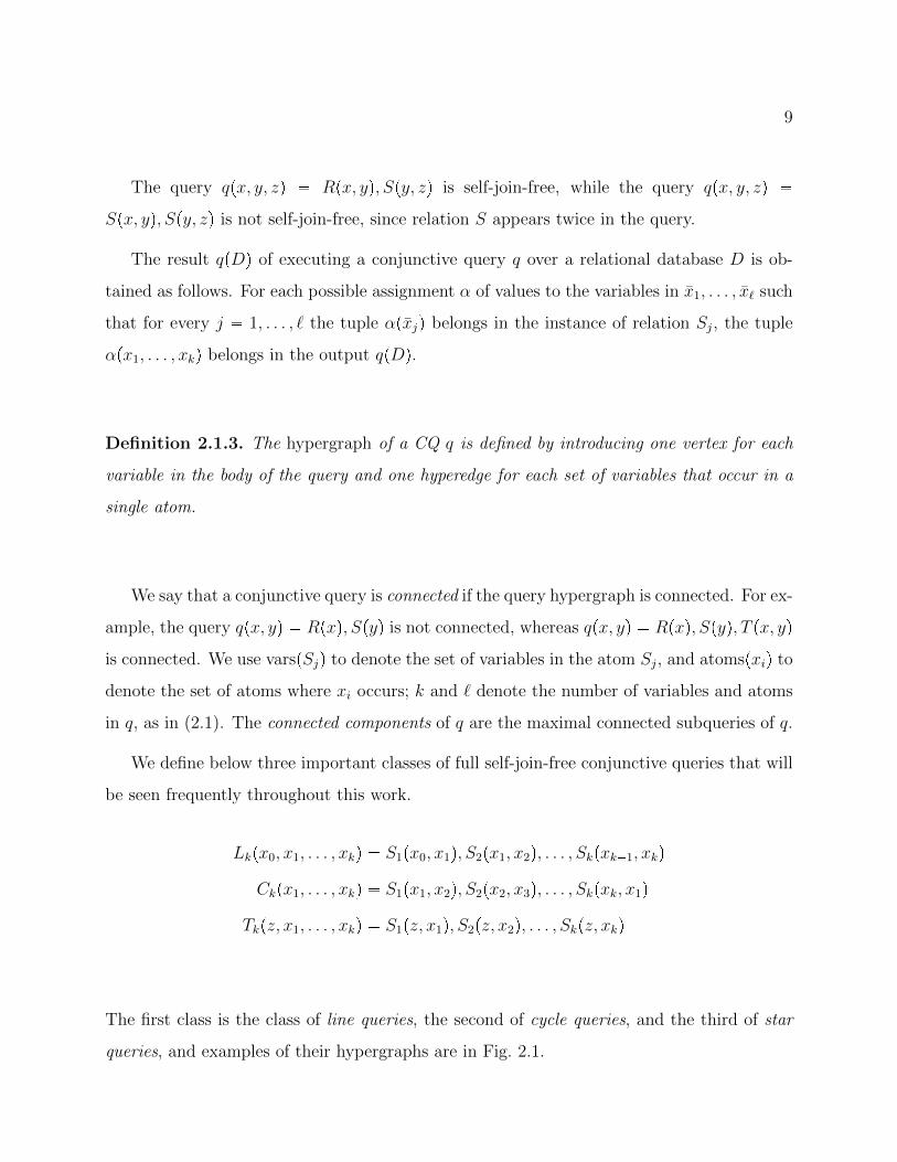
Definition 2.1.3. The hypergraph of a CQ q is defined by introducing one vertex for each
variable in the body of the query and one hyperedge for each set of variables that occur in a
single atom.
We say that a conjunctive query is connected if the query hypergraph is connected. For ex-
ample, the query qpx, yq Rpxq, Spyq is not connected, whereas qpx, yq Rpxq, Spyq, T px, yqis connected. We use varspSjq to denote the set of variables in the atom Sj, and atomspxiq to
denote the set of atoms where xi occurs; k and ` denote the number of variables and atoms
in q, as in (2.1). The connected components of q are the maximal connected subqueries of q.
We define below three important classes of full self-join-free conjunctive queries that will
be seen frequently throughout this work.
Lkpx0, x1, . . . , xkq S1px0, x1q, S2px1, x2q, . . . , Skpxk1, xkqCkpx1, . . . , xkq S1px1, x2q, S2px2, x3q, . . . , Skpxk, x1q
Tkpz, x1, . . . , xkq S1pz, x1q, S2pz, x2q, . . . , Skpz, xkq
The first class is the class of line queries, the second of cycle queries, and the third of star
queries, and examples of their hypergraphs are in Fig. 2.1.
10
x0 x1
S1
x2
S2
x3
S3
x4S4
(a) Hypergraph of L4
x1 x2
x3
S1
x4
S2
S3
S4
(b) Hypergraph of C4
z
x1
x2
x3
x4
S1
S2
S3
S4
(c) Hypergraph of T4
Figure 2.1: Examples for three different classes of conjunctive queries: (a) line queries Lk, (b) cycle queriesCk and (c) star queries Tk. The hypergraphs are depicted as graphs, since all relations are binary.
2.1.1 The Characteristic of a CQ
We introduce here a new notion, that of the characteristic of a conjunctive query, which will
be used later in this work in order to count the number of answers for queries over particular
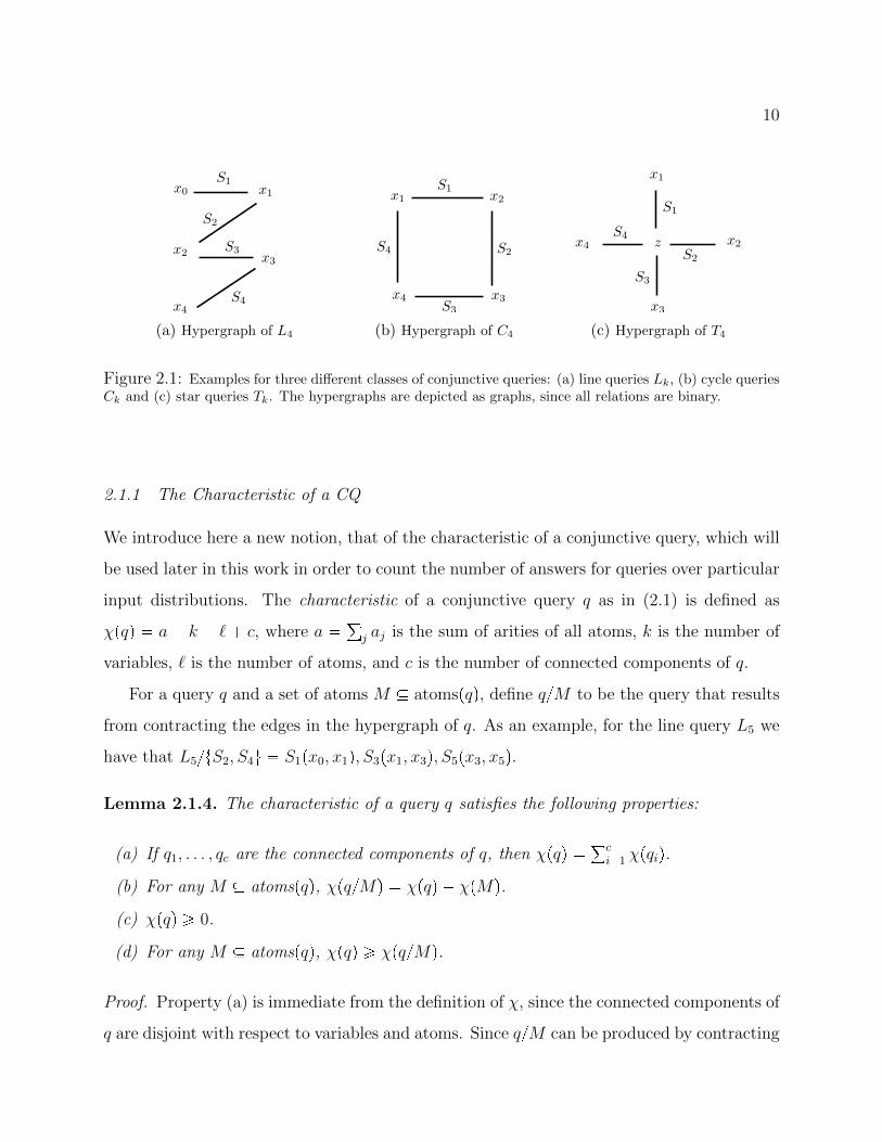
input distributions. The characteristic of a conjunctive query q as in (2.1) is defined as
χpqq a k ` c, where a °j aj is the sum of arities of all atoms, k is the number of
variables, ` is the number of atoms, and c is the number of connected components of q.
For a query q and a set of atoms M atomspqq, define qM to be the query that results
from contracting the edges in the hypergraph of q. As an example, for the line query L5 we
have that L5tS2, S4u S1px0, x1q, S3px1, x3q, S5px3, x5q.
Lemma 2.1.4. The characteristic of a query q satisfies the following properties:
(a) If q1, . . . , qc are the connected components of q, then χpqq °ci1 χpqiq.
(b) For any M atomspqq, χpqMq χpqq χpMq.(c) χpqq ¥ 0.
(d) For any M atomspqq, χpqq ¥ χpqMq.
Proof. Property (a) is immediate from the definition of χ, since the connected components of
q are disjoint with respect to variables and atoms. Since qM can be produced by contracting
11
according to each connected component of M in turn, by property (a) and induction it
suffices to show that property (b) holds in the case that M is connected. If a connected M
has kM variables, `M atoms, and total arity aM , then the query after contraction, qM , will
have the same number of connected components, kM 1 fewer variables, and the terms for
the number of atoms and total arity will be reduced by aM `M for a total reduction of
aM kM `M 1 χpMq. Thus, property (b) follows.
By property (a), it suffices to prove (c) when q is connected. If q is a single atom Sj
then χpSjq ¥ 0, since the number of variables is at most the arity aj of the atom. If q has
more than one atom, then let Sj be any such atom: then χpqq χpqSjq χpSjq ¥ χpqSjq,because χpSjq ¥ 0. Property (d) follows from (b) using the fact that χpMq ¥ 0.
For a simple illustration of property (b), consider the example above L5tS2, S4u, which
is equivalent to L3. We have χpL5q 10 6 5 1 0, and χpL3q 6 4 3 1 0,
and also χpMq 0 (because M consists of two disconnected components, S2px1, x2q and
S4px3, x4q, each with characteristic 0). For a more interesting example, consider the query
K4 whose graph is the complete graph with 4 variables:
K4 S1px1, x2q, S2px1, x3q, S3px2, x3q, S4px1, x4q, S5px2, x4q, S6px3, x4q
and denote M tS1, S2, S3u. Then K4M S4px1, x4q, S5px1, x4q, S6px1, x4q and the charac-
teristics are: χpK4q 12461 3, χpMq 6331 1, χpK4Mq 6231 2.
Finally, we define the class of tree-like queries, which will be extensively used in Chapter 6
for multi-round algorithms.
Definition 2.1.5. A conjunctive query q is tree-like if q is connected and χpqq 0.
For example, the query Lk is tree-like; in fact, a query over a binary vocabulary is tree-
like if and only if its hypergraph is a tree. An important property of tree-like queries is that
every connected subquery will be also tree-like.

12
2.1.2 The Fractional Edge Packing of a CQ
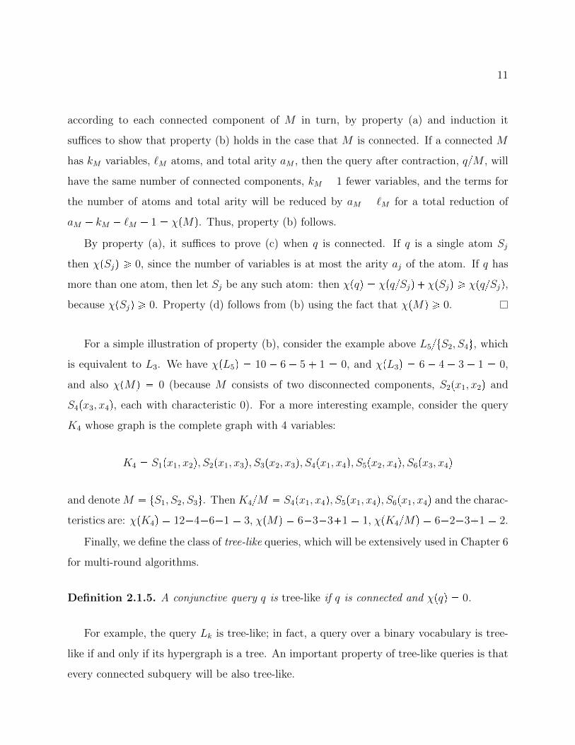
A fractional edge packing (also known as a fractional matching) of a query q is any feasible
solution u pu1, . . . , u`q of the following linear constraints:
@i P rks :¸
j:xiPvarspSjq
uj ¤ 1 (2.2)
@j P r`s : uj ¥ 0
The edge packing associates a non-negative weight uj to each atom Sj such that for
every variable xi, the sum of the weights for the atoms that contain xi do not exceed 1. If all
inequalities are satisfied as equalities by a solution to the LP, we say that the solution is tight.
The dual notion is a fractional vertex cover of q, which is a feasible solution v pv1, . . . , vkqto the following linear constraints:
@j P r`s :¸
i:xiPvarspSjq
vi ¥ 1
@i P rks : vi ¥ 0
At optimality, maxu
°j uj minv
°i vi; this quantity is denoted τ and is called the frac-
tional vertex covering number of q.
Example 2.1.6. An edge packing of the query L3 S1px1, x2q, S2px2, x3q, S3px3, x4q is any
solution to u1 ¤ 1, u1 u2 ¤ 1, u2 u3 ¤ 1 and u3 ¤ 1. In particular, the solution p1, 0, 1qis a tight edge packing; it is also an optimal packing, thus τ 2.
We also need to refer to the fractional edge cover, which is a feasible solution u pu1, . . . , u`q to the system above where ¤ is replaced by ¥ in Eq.(2.2). Every tight fractional
edge packing is a tight fractional edge cover, and vice versa. The optimal value of a fractional
edge cover is denoted ρ. The fractional edge packing and cover have no connection, and
there is no relationship between τ and ρ. For example, for q S1px, yq, S2py, zq, we have
13
Vertex Covering LP Edge Packing LP
@j P r`s :¸
i:xiPvarspSjq
vi ¥ 1 (2.3)
@i P rks : vi ¥ 0
@i P rks :¸
j:xiPvarspSjq
uj ¤ 1 (2.4)
@j P r`s : uj ¥ 0
minimize°ki1 vi maximize
°`j1 uj
Figure 2.2: The vertex covering LP of the hypergraph of a query q, and its dual edge packing LP.
τ 1 and ρ 2, while for q S1pxq, S2px, yq, S3pyq we have τ 2 and ρ 1. The
two notions coincide, however, when they are tight, meaning that a tight fractional edge
cover is also a tight fractional edge packing and vice versa. The fractional edge cover has
been used recently in several papers to prove bounds on query size and the running time of
a sequential algorithm for the query [22, 63, 64]; for the results in this paper we need the
fractional packing.
2.1.3 The Database Instance
Throughout this work, we will often focus on specific types of database instances with dif-
ferent properties.
Let R be a relation of arity r. For a tuple t over a subset of the attributes rrs that exists
in R, we define dtpRq |σtpRq| as the degree of the tuple t in relation R. In other words,
dtpRq tells us how many times the tuple t appears in the instance of relation R.1
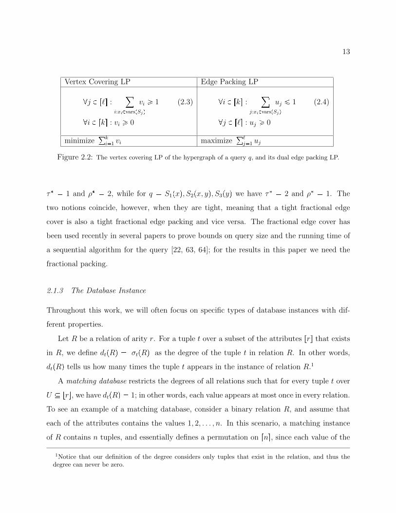
A matching database restricts the degrees of all relations such that for every tuple t over
U rrs, we have dtpRq 1; in other words, each value appears at most once in every relation.
To see an example of a matching database, consider a binary relation R, and assume that
each of the attributes contains the values 1, 2, . . . , n. In this scenario, a matching instance
of R contains n tuples, and essentially defines a permutation on rns, since each value of the
1Notice that our definition of the degree considers only tuples that exist in the relation, and thus thedegree can never be zero.
14
1
2
3
4
5
6
1
5
6
2
3
4
(a) A depiction of a matching instance for rela-tion Rpx, yq as a bipartite matching
1
1
2
3
4
5
6
(b) A depiction of a (maximally) skewed instancefor relation Rpx, yq
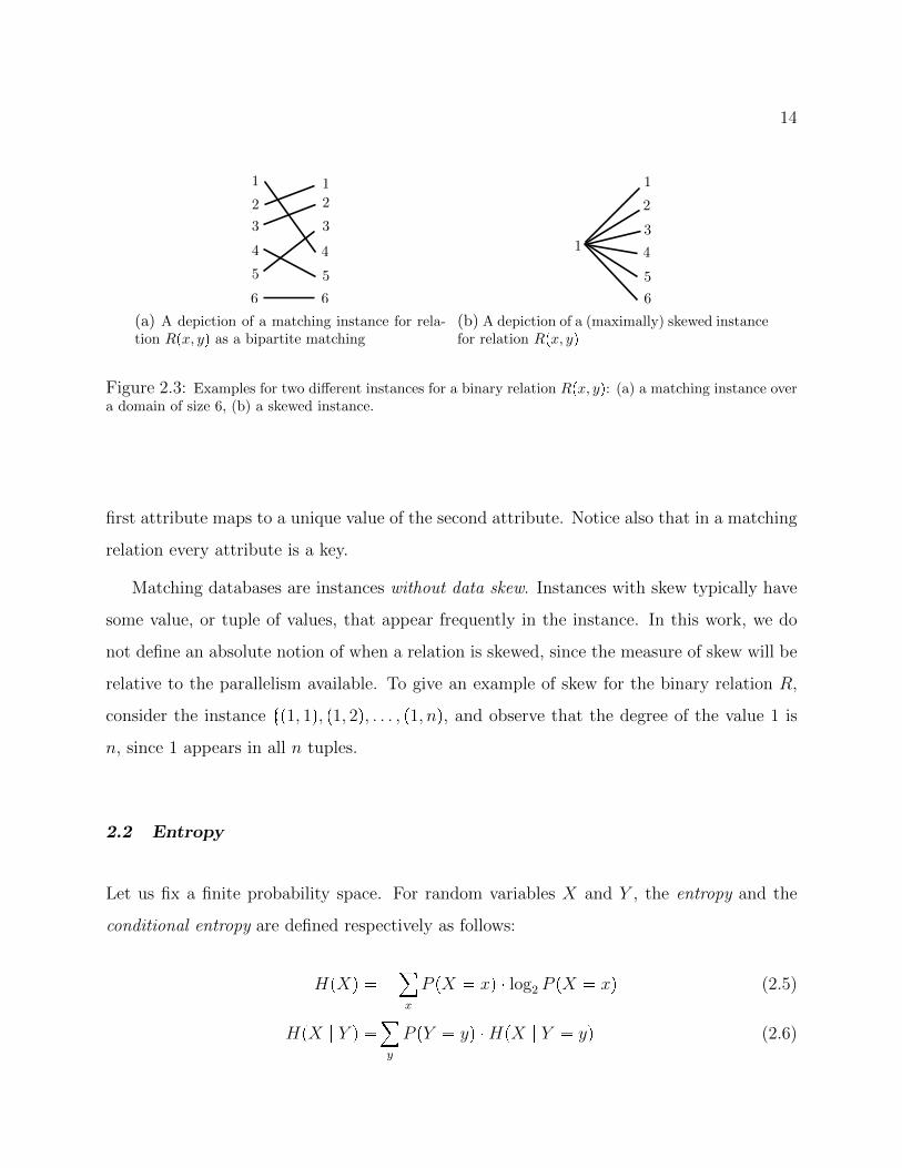
Figure 2.3: Examples for two different instances for a binary relation Rpx, yq: (a) a matching instance overa domain of size 6, (b) a skewed instance.
first attribute maps to a unique value of the second attribute. Notice also that in a matching
relation every attribute is a key.
Matching databases are instances without data skew. Instances with skew typically have
some value, or tuple of values, that appear frequently in the instance. In this work, we do
not define an absolute notion of when a relation is skewed, since the measure of skew will be
relative to the parallelism available. To give an example of skew for the binary relation R,
consider the instance tp1, 1q, p1, 2q, . . . , p1, nq, and observe that the degree of the value 1 is
n, since 1 appears in all n tuples.
2.2 Entropy
Let us fix a finite probability space. For random variables X and Y , the entropy and the
conditional entropy are defined respectively as follows:
HpXq ¸x
P pX xq log2 P pX xq (2.5)
HpX | Y q ¸y
P pY yq HpX | Y yq (2.6)

15
The entropy satisfies the following two basic inequalities:
HpX | Y q ¤ HpXqHpX, Y q HpX | Y q HpY q (2.7)
Assuming additionally that X has a support of size n, we have:
HpXq ¤ log2 n (2.8)
2.3 Yao’s Principle
The lower bounds that we show in this work apply not only to deterministic algorithms, but
to randomized algorithms as well. To prove lower bounds for randomized algorithms, we use
Yao’s Principle [83]. In the setting of answering conjunctive queries, Yao’s principle can be
stated as follows.
Let P be any probability space from which we choose a database instance I, such that
every deterministic algorithm fails to compute qpIq correctly with probability ¥ 1δ. Then,
for every randomized algorithm, there exists a database instance I 1 such that the algorithm
fails to compute qpI 1q correctly with probability ¥ 1 δ, where the probability is over the
random choices of the algorithm.
In other words, if we want to prove a lower bound for randomized algorithms, it suffices to
construct a probability distribution over instances for which any deterministic algorithm fails.
As we will see, Yao’s principle allows us to prove strong lower bounds for the communication
load, even in the case where we allow communication to take arbitrary form.
2.4 Friedgut’s Inequality
Friedgut [41] introduces a powerful class of inequalities, which will provide a useful tool for
proving lower bounds. Each inequality is described by a hypergraph, but since we work with
conjunctive queries, we will describe the inequality using query terminology (and thus the
16
hypergraph will be the query hypergraph). Fix a query q as in (2.1), and let n ¡ 0. For every
atom Sjpxjq of arity aj, we introduce a set of naj variables wjpajq ¥ 0, where aj P rnsaj . If
a P rnsa, we denote by aj the vector of size aj that results from projecting on the variables
of the relation Sj. Let u pu1, . . . , u`q be a fractional edge cover for q. Then:
¸aPrnsk
¹j1
wjpajq ¤¹j1
¸
ajPrnsaj
wjpajq1uj uj
(2.9)
We illustrate Friedgut’s inequality on the queries C3 and L3:
C3px, y, zq S1px, yq, S2py, zq, S3pz, xqL3px, y, z, wq S1px, yq, S2py, zq, S3pz, wq (2.10)
Consider the cover p12, 12, 12q for C3, and the cover p1, 0, 1q for L3. Then, we obtain the
following inequalities, where α, β, γ stand for w1, w2, w3 respectively:
¸x,y,zPrns
αxy βyz γzx ¤d ¸
x,yPrns
α2xy
¸y,zPrns
β2yz
¸z,xPrns
γ2zx
¸x,y,z,wPrns
αxy βyz γzw ¤¸
x,yPrns
αxy maxy,zPrns
βyz ¸
z,wPrns
γzw
where we used the fact that limuÑ0p°β
1uyzqu max βyz.
Friedgut’s inequalities immediately imply a well known result developed in a series of
papers [46, 22, 63, 64] that gives an upper bound on the size of a query answer as a function
on the cardinality of the relations. For example in the case of C3, consider an instance
S1, S2, S3, and set αxy 1 if px, yq P S1, otherwise αxy 0 (and similarly for βyz, γzx). We
obtain then |C3| ¤a|S1| |S2| |S3|. Note that all these results are expressed in terms of a
fractional edge cover. When we apply Friedgut’s inequality in Chapter 4 to a fractional edge
packing, we ensure that the packing is tight.
17
Chapter 3
THE MASSIVELY PARALLEL COMPUTATION MODEL
In this chapter, we introduce the Massively Parallel Computation model (MPC), a the-
oretical model that allows us to analyze algorithms in massively parallel environments. We
first give the formal description of the model in Section 3.1, where we also discuss some
observations and simplifying assumptions. In Section 3.2, we present a comparison of the
MPC model with previous parallel models, and discuss our modeling choices along various
axes. Finally in Section 3.3, we study the connections of the MPC model with the area of
communication complexity.
3.1 The MPC Model: Computation and Parameters
In the MPC model, introduced in [23, 24], computation is performed by p servers, or pro-
cessors, connected by a complete network of private channels. Each server can communicate
with any other server in an indistinguishable way. The servers run the parallel algorithm in
communication steps, or rounds, where each round consists of two distinct phases1:
Communication Phase: The servers exchange data, each by communicating with all other
servers (both sending and receiving data).
Computation Phase: Each server performs computation on the local data it has received
during all previous rounds.
The input data of size M (in bits) is initially uniformly partitioned among the p servers,
i.e. each server stores Mp bits of the data: this describes the way the data is typically par-
1In earlier versions of our work on parallel processing [55, 12], we had a third phase called the broadcastphase.

18
titioned in any distributed storage system, for example in HDFS [71]. We do not make any
particular assumptions on whether the data is partitioned according to a specific scheme.
Thus, any parallel algorithm must work for an arbitrary data partition, while any lower
bound can use a worst-case initial distribution of the data. We should note here that spe-
cific partitioning schemes (for example hash-partitioning a relation according to a specific
attribute) can help design better parallel algorithms, but this is not something we consider
in this dissertation.
After the computation is completed, the output data is present in the union of the output
of the p servers.
The complexity of a parallel algorithm in the MPC model is captured by two basic
parameters in the computation:
The number of rounds r. This parameter captures the number of synchronization barri-
ers that an algorithm requires during execution. A smaller number of rounds means
that the algorithm can run with less synchronization.
The maximum load L. This parameter captures the maximum load among all servers at
any round, where the load is the amount of data (in bits) received by a server during
a particular round. Let Ls,k denote the number of bits that server s receives during
round k. Then, we define formally L as:
L maxk1,...,r
t maxs1,...,p
Ls,ku
The reader should notice that the MPC model does not restrict or capture the running
time of the computation at each server; in other words, the servers can be as computationally
powerful as we would like. This modeling choice means that our lower bounds must be
information-theoretic, since they are based on how much data is available to each server and
not on how much computation is needed to output the desired result. On the other hand,
the algorithms that we present throughout this work are always polynomially bounded and
19
round 1 round 2
communication communication
...
... ... ... ...
round rround 3
server 1
server 2
server 3
server p
computation computation computation
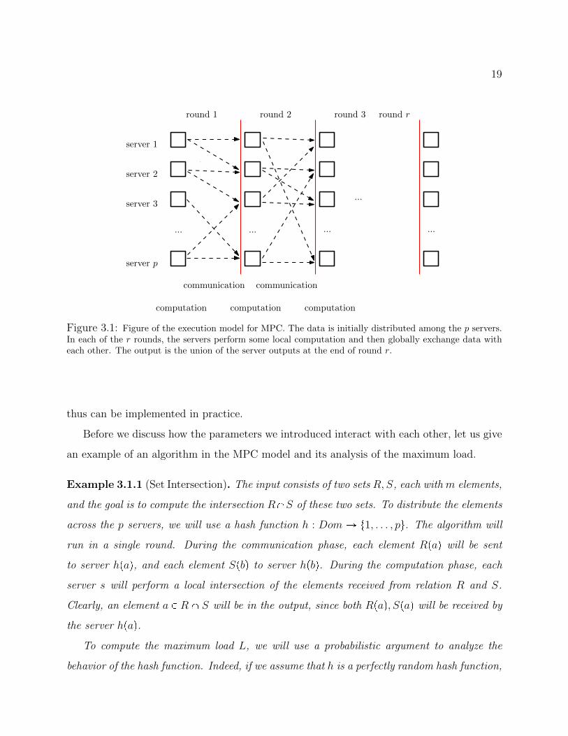
Figure 3.1: Figure of the execution model for MPC. The data is initially distributed among the p servers.In each of the r rounds, the servers perform some local computation and then globally exchange data witheach other. The output is the union of the server outputs at the end of round r.
thus can be implemented in practice.
Before we discuss how the parameters we introduced interact with each other, let us give
an example of an algorithm in the MPC model and its analysis of the maximum load.
Example 3.1.1 (Set Intersection). The input consists of two sets R, S, each with m elements,
and the goal is to compute the intersection RXS of these two sets. To distribute the elements
across the p servers, we will use a hash function h : Dom Ñ t1, . . . , pu. The algorithm will
run in a single round. During the communication phase, each element Rpaq will be sent
to server hpaq, and each element Spbq to server hpbq. During the computation phase, each
server s will perform a local intersection of the elements received from relation R and S.
Clearly, an element a P RX S will be in the output, since both Rpaq, Spaq will be received by
the server hpaq.To compute the maximum load L, we will use a probabilistic argument to analyze the
behavior of the hash function. Indeed, if we assume that h is a perfectly random hash function,
20
it can be shown that the load (in number of elements, not bits) will be Opmpq with high
probability when m " p.
Let us now discuss the interaction between the number of rounds, the input size and
the load to provide some intuition on our modeling choices. Normally, the entire data is
exchanged during the first communication round, so the load L is at least Mp. Thus, the
set intersection algorithm from the above example is asymptotically optimal. On the other
hand, if we allowed a load L M , then any problem can solved trivially in one round by
simply sending the entire data to server 1, then computing the answer locally. In this case
though, we failed to exploit the available parallelism of the p machines. The typical loads in
most of our analyses will be of the form Mp1ε, for some parameter 0 ¤ ε 1 that depends
on the query (we call the parameter ε the space exponent, see Subsection 4.4.2).
Observe also that if we allowed the number of rounds to reach r p, any problem can
be solved trivially in p rounds by sending at each round Mp bits of data to server 1, until
this server accumulates the entire data. In this thesis, we will mostly focus on algorithms
that need a constant number of rounds, r Op1q, to perform the necessary computation.
3.1.1 Computing Queries in the MPC model
In this dissertation, the main focus will be the computation of full conjunctive queries, as
defined in (2.1). As an example, for the triangle query Rpx, yq, Spy, zq, T pz, xq, we want
to output all the triangles. It is straightforward that an MPC algorithm that computes all
triangles will be able to answer the corresponding boolean query, i.e. whether there exist any
triangles, but the opposite does not hold, since computing the decision version may require
a more efficient algorithm. Computing all answers further allows us to count the answers
(for example count the number of triangles), but again the counting version of a query may
allow for a better parallel algorithm.
We discuss next two assumptions that will allow us to simplify the treatment of conjunc-
tive queries in the MPC model: the first one concerns the existence of self-joins, and the
21
second the initial partitioning of the input.
Self-Joins. Instead of studying the computation of any full conjunctive query, we can focus
only on algorithms and bounds for self-join-free queries without any loss of generality.
To see this, let q be any conjunctive query, and denote q1 the query obtained from q
by giving distinct names to repeated occurrences of the same relations (hence q is self-
join-free). For example, consider the query q Spx, yq, Spy, zq, Spz, xq, which computes all
triangles in a directed graph with edge set S. Then, q1 will be the self-join-free triangle query
S1px, yq, S2py, zq, S3pz, xq.Clearly, if we have an MPC algorithm A1 for q1, we can apply this algorithm directly to
obtain an algorithm for q by essentially ‘copying’ the relations that appear multiple times in
the body of the query. The new algorithm will have the same load as A1 when executed on
an input that is at most ` times larger than the original input (recall that ` is the number
of relations). In our example, we would copy relation S of size M to create three replicas
S1, S2, S3, each of size M , then execute the triangle query on an input 3 times as large, and
finally obtain the output answers.
Conversely, suppose that we have an algorithm A for the query q with self-joins. We
construct an algorithm A1 for q1 as follows. Suppose that relation S has k occurrences in
q and has k distinct names S1, . . . , Sk in q1. For each atom Sipx, y, z, . . .q, algorithm A1
renames every tuple Sipa, b, c, . . .q into Spxa, xy, xb, yy, xc, zy, . . .q. That is, each value a in
the first column is replaced by the pair xa, xy, where x is the variable occurring in that
column, and similarly for all other columns. This copy operation can be performed locally
by all servers, without any additional communication cost. The resulting relation S will be
essentially a ‘union’ of the k relations, but where we remember the variable mapping for each
value. We can execute then A on the constructed input, which will be exactly the same size
as the original input. In the end, we have to perform a filtering step to return the correct
output for q1: if the head variables of q are x, y, . . . and an output tuple is pxa, uy, xb, vy, . . . q,then the algorithm needs to check that x u, y v, . . . , and only then return the tuple.
22
Input Partitioning. The MPC model assumes an arbitrary initial distribution of the
input relations in the p servers. Our algorithms in the next sections are able to operate with
any distribution, since they operate per tuple (and some possibly side information). In order
to show lower bounds, however, it will be convenient to use the assumption that initially
each relation Sj is stored in a separate server, called an input server. During the first round,
the input servers send messages to the p servers, but in subsequent rounds they are no longer
used in the computation. All lower bounds in this paper assume that the relations Sj are
given on separate input servers.
We next show that if we have a lower bound on the maximum load for the model with
separate input servers, the bound carries over immediately to the standard MPC model for
the class of self-join-free conjunctive queries.
Lemma 3.1.2. Let q be a self-join-free conjunctive query q with input sizes M pM1, . . . ,M`q. Let A be an algorithm that computes q in r rounds with load LpM, pq in
the standard MPC model. Then, there exists an algorithm A1 that computes q in the input
server model in r rounds and load LpM, pq Mp, where M °`j1Mj is the total size of
the input.
Proof. We will construct an algorithm A1 over the input server model as follows. The input
server j will take the input relation Sj, and simply split it into pMjM chunks: each chunk
now contains Mp data, so we can simulate each of the p servers in the first round of the
MPC model. Notice that during the first round we also have to send the initial chunk of the
input relation to the corresponding server (which is the data that the server would contain
during initialization for A). In subsequent rounds ¥ 2, algorithm A1 behaves exactly the
same as algorithm A. We can observe now that algorithm A1 requires r rounds, and achieves
a load of LpM, pq Mp.
Say that we show a lower bound LpM, pq for the input server model such that LpM, pq ¥2Mp (this assumption holds for every lower bound that we show, since intuitively the input
must be distributed once among the servers to do any computation). From the above result,
23
this implies that every algorithm for the standard MPC model using the same number of
rounds requires a load of at least LpM, pq2. Thus, it suffices to prove our lower bounds
assuming that each input relation is stored in a separate input server. Observe that this
model is even more powerful, because an input server has now access to the entire relation
Sj, and can therefore perform some global computation on Sj, for example compute statistics,
find outliers, etc., which are common in practice.
3.1.2 The tuple-based MPC model
The MPC model, as defined in the previous sections, allows arbitrary communication among
the servers at every round, which makes the theoretical analysis of multi-round algorithms
a very hard task. Thus, in order to show lower bounds for the case of multiple rounds, we
will need to restrict the form of communication in the MPC model; to do this, we define a
restriction of the MPC model that we call the tuple-based MPC model. More precisely, the
tuple-based MPC model will impose a particular structure on what kind of messages can be
exchanged among the servers.
Let I be the input database instance, q be the query we want to compute, and A an
algorithm. For a server s P rps, we denote by msg1jÑspA, Iq the message sent during round 1
by the input server for Sj to the server s, and by msgksÑs1pA, Iq the message sent to server
s1 from server s at round k ¥ 2. Let msg1spA, Iq pmsg1
1ÑspA, Iq, . . . ,msg1`ÑspA, Iqq and
msgkspA, Iq pmsgk1ÑspA, Iq, . . . ,msgkpÑspA, Iqq for any round k ¥ 2.
Further, we define msg¤ks pA, iq to be the vector of messages received by server s during
the first k rounds, and msg¤kpA, iq pmsg¤k1 pA, iq, . . . ,msg¤kp pA, iqq.Define a join tuple to be any tuple in q1pIq, where q1 is any connected subquery of
q. An algorithm A in the tuple-based MPC model has the following two restrictions on
communication during rounds k ¥ 2, for every server s
• the message msgksÑs1pA, Iq is a set of join tuples.
• for every join tuple t, the server s decides whether to include t in msgksÑs1pA, Iq based

24
only on the parameters t, s, s1, r, and the messages msg1jÑspA, Iq for all j such that t
contains a base tuple in Sj.
The restricted model still allows unrestricted communication during the first round; the
information msg1spA, Iq received by server s in the first round is available throughout the
computation. However, during the following rounds, server s can only send messages con-
sisting of join tuples, and, moreover, the destination of these join tuples can depend only on
the tuple itself and on msg1spA, Iq.
The restriction of communication to join tuples (except for the first round during which
arbitrary, e.g. statistical, information can be sent) is natural and the tuple-based MPC
model captures a wide variety of algorithms including those based on MapReduce. Since
the servers can perform arbitrary inferences based on the messages that they receive, even a
limitation to messages that are join tuples starting in the second round, without a restriction
on how they are routed, would still essentially have been equivalent to the fully general MPC
model. For example, any server wishing to send a sequence of bits to another server can
encode the bits using a sequence of tuples that the two exchanged in previous rounds, or
(with slight loss in efficiency) using the understanding that the tuples themselves are not
important, but some arbitrary fixed Boolean function of those tuples is the true message
being communicated. This explains the need for the condition on routing tuples that the
tuple-based MPC model imposes.
3.2 Comparison of MPC to other Parallel Models
In this section, we present several theoretical models that have been developed for parallel
computation, and compare them with the MPC model, noting both the modeling similarities
and differences. We will discuss only models that capture shared-nothing architectures [76]:
in such an architecture, every machine has its own memory and there is no shared memory
available. This does not include for example the first parallel model, the Parallel Random-
Access Machine (PRAM) model, where a number of processors share an unbounded memory
25
and can operate in a synchronous way on a shared input. 2 Further, we discuss models
that are synchronous, in the sense that the computation and communication proceeds in
well-defined rounds. The comparison will be across five different axes:
1. Number of servers. The number of servers can be an explicit parameter (as in the
MPC model), or it can be chosen by the algorithm according to the input data.
2. Number of rounds. This parameter counts the number of rounds, or synchronization
barriers, during computation. Reducing the number of steps is important in terms of
performance, because of the overhead of synchronization and the presence of stragglers,
which are machines that finish slower than the rest.
3. Memory bound. This parameter models how much memory is available to each server,
or how much data (load) each server is allowed to receive during computation. This
restriction captures the parallelism in computation: the smaller the amount of data
each server receives, the more parallel the task is.
4. Communication. This parameter captures how much data is exchanged during the
communication between servers. There are many different ways communication is
modeled: one can choose to count the total amount of data exchanged, or model it
indirectly by looking at the number of servers and the memory bound.
5. Computation. Some models require that the computation is polynomial, or that the
running time is counted towards measuring the parallel complexity.
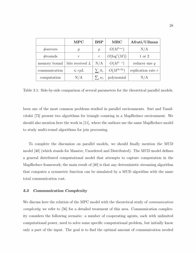
The BSP Model. To address some of the issues of the PRAM model, Valiant [77] intro-
duced the Bulk Synchronous Parallel (BSP) model. A BSP algorithm runs in supersteps:
each superstep consists of local computation and asynchronous communication, followed by
a synchronization barrier. The BSP model abstracts the communication in every superstep
by introducing the notion of the h-relation, which is defined as a communication pattern
where the maximum number of incoming or outgoing messages per machine is h. The cost
2Immerman showed in [51] that computing an expression in first-order logic (and thus evaluating con-junctive queries) requires constant time in PRAM, earning the name ”embarrassingly parallel”.
26
of a superstep i consists of three components: the cost of synchronization (a constant `), the
communication cost hi (the size of the hi-relation) and the computation cost wi (measured
as the longest running local computation). The cost of a BSP algorithm is computed as a
weighted sum of these terms over all steps:°ipwi ghi `q.
The MPC model is similar to the BSP model, but we remove the computation cost from
consideration, and also do not allow any form of asynchronous communication; this allows
us to prove lower bounds on the cost by using information-theoretic arguments. Moreover,
instead of measuring the total communication°i hi over all supersteps, the MPC model
considers the largest value of hi, which the load L.
Related to the BSP model is the CONGEST model [42] for distributed computing; the
difference between the two models is that the CONGEST model considers a communication
graph that may not be a full clique, as in the BSP model.
The LogP Model. The LogP model, introduced in [36], builds on the BSP model by
using more system parameters to model the execution. L denotes the latency of the com-
munication medium, o the overhead of sending and receiving a message, g denotes the gap
required between two send/receive operation, and finally P is the number of processing units.
Following the introduction of the MapReduce model [37], several theoretical models were
introduced in the literature to capture computation in this setting. MapReduce is a restricted
version of the BSP model, where synchronization occurs at every step, and uses a simple
programming model inspired by functional programming. In its vanilla version, the user
defines two functions: map and reduce. The map function is applied on a single data item
x of the input and returns a key-value pair pk, vq. The reduce function is applied to a list of
items with the same key, pk, rv1, . . . , vmsq and returns a new list of values. During runtime,
the system applies in parallel the map function, then performs a shuffle step that collects all
key-value pairs with the same key to the same location (reducer); finally, the reduce function
is applied in parallel to each key-group.
27
The MRC model. In order to capture computation in the MapReduce framework, the
authors in [54] define the MapReduce class (MRC) of algorithms. Denoting by M the size of
the input in bits, the model restricts both the memory per reducer/machine and the number
of machines/reducers to OpM1εq, for some constant ε ¡ 0. Observe that this means that
the number of machines (or reducers in their case) is not explicitly defined. The machines
can perform only polynomial time computations, and further the number of rounds must
be limited to OplogcpMqq for some constant c. In a related work [45], the authors use an
explicit parameter B to bound the memory of each reducer, and use the total amount of
communication C and number of rounds R as parameters that capture the complexity of a
MapReduce algorithm.
Both works do not consider problems related to query processing, but tasks such as
sorting or the Minimum Spanning Tree problem. Moreover, they provide no lower bounds
on the communication or round complexity.
The Afrati-Ullman model. In [14], Afrati and Ullman develop a model for MapReduce
where the main parameter is an upper bound q on the number of input tuples a reducer
can receive, called reducer size; this is the same as the memory per node. Given an input
of size M , a MapReduce algorithm is restricted to deterministically send each input tuple
independently to some reducer, which will then produce all the outputs that can be extracted
from the received tuples. If qi ¤ q is the number of inputs assigned to the i-th reducer, where
i 1, . . . , p, the replication rate of the algorithm is r °pi1 qiM . The replication rate
captures the communication cost of the algorithm.
In previous works [15, 10], the authors considered the total communication as the com-
plexity measure instead of the memory per machine, and studied the problems of multiway
joins and enumeration of subgraph patterns in a graph. The authors study the tradeoff
between r and q for various settings, including Hamming distance (see also [13] for a deeper
investigation of Hamming distance algorithms), matrix multiplication, triangle finding, and
multiway joins. In particular, the problem of enumerating and/or counting triangles has
28
MPC BSP MRC Afrati/Ullman
#servers p p OpM1εq N/A
#rounds r r OplogcpMqq 1 or 2
memory bound bits received L N/A OpM1εq reducer size q
communication ¤ rpL°i hi OpM22εq replication rate r
computation N/A°iwi polynomial N/A
Table 3.1: Side-by-side comparison of several parameters for the theoretical parallel models.
been one of the most common problems studied in parallel environments. Suri and Vassil-
vitskii [73] present two algorithms for triangle counting in a MapReduce environment. We
should also mention here the work in [11], where the authors use the same MapReduce model
to study multi-round algorithms for join processing.
To complete the discussion on parallel models, we should finally mention the MUD
model [40] (which stands for Massive, Unordered and Distributed). The MUD model defines
a general distributed computational model that attempts to capture computation in the
MapReduce framework; the main result of [40] is that any deterministic streaming algorithm
that computes a symmetric function can be simulated by a MUD algorithm with the same
total communication cost.
3.3 Communication Complexity
We discuss here the relation of the MPC model with the theoretical study of communication
complexity; we refer to [56] for a detailed treatment of this area. Communication complex-
ity considers the following scenario: a number of cooperating agents, each with unlimited
computational power, need to solve some specific computational problem, but initially know
only a part of the input. The goal is to find the optimal amount of communication needed
29
(in bits) to solve the problem.
There are many versions of this problem, depending on the number of agents, whether
randomization is used or how the input is distributed among the agents, but the model
closer to MPC is Number-In-Hand (NIH) multiparty communication complexity (see [68] for
example), where initially each agent receives a part of the input that is not shared with any
other agent. Although several computational tasks have been considered in this model, such
as set-disjointness or string equality, query processing has not been much studied. It should
be noted here that lower bounds for NIH communication complexity are extensively used
to obtain results in other areas, such as lower bounds on the space requirements for data
streaming algorithms (e.g. [18]).
There are three variations on the communication mode that is being used. In the black-
board model, any message sent by an agent is written to a blackboard visible to all other
agents. In the coordinator model, an additional agent, called the coordinator, receives no
input, but all agents can communicate only with the coordinator and not with each other
directly. In both of these modes, at least one agent has access to all communication among
agents; hence, any computational task with input of size M and output of size O can be
computed using no more than MO bits of communication. The third mode is the message-
passing model, where there is a private 2-way communication channel connecting any two
agents, and every message is privately sent to a specific agent. There has been a recent line
of work ([80, 30]) investigating the communication complexity of several tasks in this setting.
In [80], the authors investigate various statistical and graph problems (such as connectivity,
bipartiteness, degree computation), and show that for most tasks the simple algorithm of
communicating all data to a single location is almost optimal. In [30], the authors study the
problem of set intersection, which can be seen as a case of join computation.
Since the communication in the MPC model is point-to-point private communication,
the more related mode is the message passing model. However, there is still a key difference:
the MPC model measures the communication per agent/machine and per round instead of
measuring the total communication. As a result, in many of the computational tasks we

30
analyze in the next sections, we obtain lower bounds were the total communication is of the
form M1δ, which is much larger than a protocol in the NIH model would require. Thus, by
measuring communication in a more fine-grained way, we can obtain stronger lower bounds.
To complete the discussion on communication complexity, we should also mention the
work in [47], where the authors examine the 2-party NIH communication complexity for
distributed set-joins, which includes multiway joins as a special case.
31
Chapter 4
COMPUTING JOIN QUERIES IN ONE STEP WITHOUTSKEW
In this chapter, we present the main result of this dissertation. We study the complexity
of computing conjunctive queries in the MPC model for a single communication round under
the assumption that the input data has no skew. We show that under this assumption, there
exists an algorithm, called the HyperCube algorithm, that computes any conjunctive query
by achieving the optimal load.
Recall that we represent a full conjunctive query q as:
qpx1, . . . , xkq S1px1q, . . . , S`px`q
where k is the number of variables and ` is the number of atoms. Throughout this chapter,
we will assume that the input servers know the cardinalities m1, . . . ,m` of the relations
S1, . . . , S`. We denote m pm1, . . . ,m`q the vector of cardinalities, and M pM1, . . . ,M`qthe vector of the sizes expressed in bits, where Mj ajmj log n, n is the size of the domain
of each attribute, and aj the arity of each atom.
Given the size information, how well can an algorithm do in a single communication
round? The central result we show is that a particular type of algorithm, which we call the
HyperCube algorithm, if parametrized correctly can achieve optimal load for any conjunc-
tive query q. However, our result does not hold for any input data, but for data without
skew. We will give a precise definition of skew later in this chapter, but intuitively no skew
means that no value in the input data appears many times.
Recall that a database is a matching database if each relation has degree bounded by 1
(i.e. the frequency of each value is exactly 1 for each relation). Our lower bounds hold for

32
an input distribution that consists of such matching databases. One can view a matching
database as input with the least amount of skew possible. The upper bound, and in particular
the load analysis for the HyperCube algorithm, hold not only for matching databases,
but in general for databases with a small amount of skew, which we will formally define
in Section 4.1. This means that the HyperCube algorithm has some resilience in skew, and
we can quantify exactly how much this resilience is.
4.1 The HyperCube Algorithm
We describe here the HyperCube algorithm, which we will use to compute any conjunctive
query in one round. This algorithm was introduced by Afrati and Ullman [9] in a MapReduce
setting, and is similar to an algorithm by Suri and Vassilvitskii [73] to count the number
of triangles in graphs. The idea though can be traced much earlier in time, to a work by
Ganguly [43] on parallel processing of Datalog programs. We call this the HyperCube
(HC) algorithm, following [23], but it can also be found in the literature as the Shares
algorithm [9].
The algorithm is simple in principle, and the core idea is to perform communication by
doing a smart routing of the input tuples. The communication phase of the algorithm is
highly distributed, since the destination of each input tuple depends only on the content of
the specific tuple, the size M of the relations and the query q. Thus, the algorithm can be
easily implemented in almost any distributed or parallel computing environment.
The HC Algorithm. We initially assign to each variable xi, where i 1, . . . , k, a share
pi, such that±k
i1 pi p. Each server is then represented by a distinct point y P P , where
P rp1s rp2s; in other words, servers are mapped into points of a k-dimensional
hypercube.1
• Communication: We use k independently chosen hash functions hi : rns Ñ rpis and
1This is where the algorithm takes its name from.
33
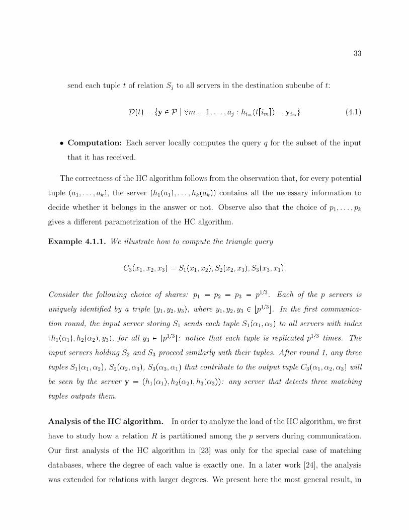
send each tuple t of relation Sj to all servers in the destination subcube of t:
Dptq ty P P | @m 1, . . . , aj : himptrimsq yimu (4.1)
• Computation: Each server locally computes the query q for the subset of the input
that it has received.
The correctness of the HC algorithm follows from the observation that, for every potential
tuple pa1, . . . , akq, the server ph1pa1q, . . . , hkpakqq contains all the necessary information to
decide whether it belongs in the answer or not. Observe also that the choice of p1, . . . , pk
gives a different parametrization of the HC algorithm.
Example 4.1.1. We illustrate how to compute the triangle query
C3px1, x2, x3q S1px1, x2q, S2px2, x3q, S3px3, x1q.
Consider the following choice of shares: p1 p2 p3 p13. Each of the p servers is
uniquely identified by a triple py1, y2, y3q, where y1, y2, y3 P rp13s. In the first communica-
tion round, the input server storing S1 sends each tuple S1pα1, α2q to all servers with index
ph1pα1q, h2pα2q, y3q, for all y3 P rp13s: notice that each tuple is replicated p13 times. The
input servers holding S2 and S3 proceed similarly with their tuples. After round 1, any three
tuples S1pα1, α2q, S2pα2, α3q, S3pα3, α1q that contribute to the output tuple C3pα1, α2, α3q will
be seen by the server y ph1pα1q, h2pα2q, h3pα3qq: any server that detects three matching
tuples outputs them.
Analysis of the HC algorithm. In order to analyze the load of the HC algorithm, we first
have to study how a relation R is partitioned among the p servers during communication.
Our first analysis of the HC algorithm in [23] was only for the special case of matching
databases, where the degree of each value is exactly one. In a later work [24], the analysis
was extended for relations with larger degrees. We present here the most general result, in

34
other words we specify the largest possible degree for which the distribution of the tuples
will not be influenced by skew. The analysis is based on the following lemma about hashing,
which we prove in detail in Section A.2.
Lemma 4.1.2. Let RpA1, . . . , Arq be a relation of arity r of size m. Let p1, . . . , pr be integers
and let p ±i pi. Suppose that we hash each tuple pa1, . . . , arq to the bin ph1pa1q, . . . , hrparqq,where h1, . . . , hr are independent and perfectly random hash functions from the domain n to
p1, . . . , pr respectively. Then:
1. The expected load in every bin is mp.
2. Suppose that for every tuple J over U rrs we have dJpRq ¤ mα|U |
±iPU pi
for some
constant α ¡ 0. Then the probability that the maximum load exceeds Opmpq is expo-
nentially small in p.2
Using the above lemma, we can now prove the following statement on the behavior of
the HC algorithm.
Corollary 4.1.3. Let p pp1, . . . , pkq be the shares of the HC algorithm. Suppose that for
every relation Sj and every tuple J over U rajs we have dJpSjq ¤ mj
α|U |±
iPU pifor some
constant α ¡ 0. Then with high probability the maximum load per server is
O
maxj
Mj±i:iPSj
pi
Choosing the Shares. We have not discussed yet how to choose the best shares for the
HC algorithm. The above analysis provided us with a tool that allows us to make the best
possible choice. Afrati and Ullman in [9] compute the shares by optimizing the total load°jmj
±i:iPSj
pi subject to the constraint±
i pi 1, which is a non-linear system that can
be solved using Lagrange multipliers. Our approach is to optimize the maximum load per
relation, L maxjmj±
i:iPSjpi; the total load per server is ¤ `L. This leads to a linear
2The notation O hides logppq factors.
35
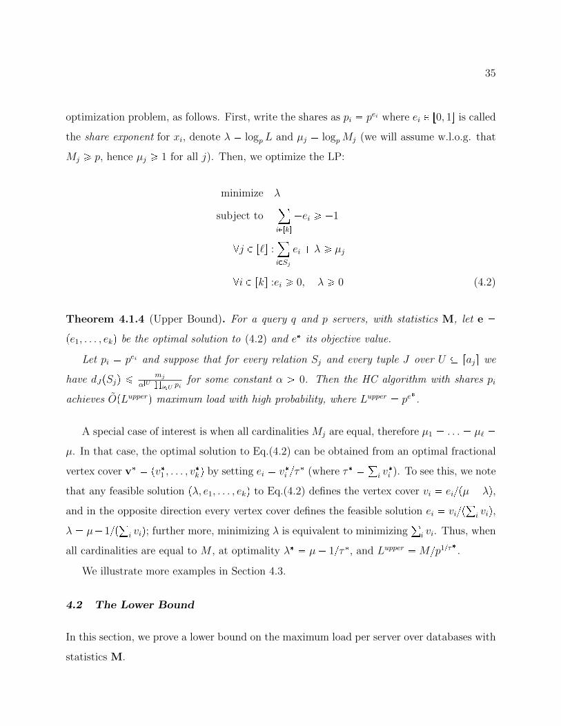
optimization problem, as follows. First, write the shares as pi pei where ei P r0, 1s is called
the share exponent for xi, denote λ logp L and µj logpMj (we will assume w.l.o.g. that
Mj ¥ p, hence µj ¥ 1 for all j). Then, we optimize the LP:
minimize λ
subject to¸iPrks
ei ¥ 1
@j P r`s :¸iPSj
ei λ ¥ µj
@i P rks :ei ¥ 0, λ ¥ 0 (4.2)
Theorem 4.1.4 (Upper Bound). For a query q and p servers, with statistics M, let e pe1, . . . , ekq be the optimal solution to (4.2) and e its objective value.
Let pi pei and suppose that for every relation Sj and every tuple J over U rajs we
have dJpSjq ¤ mj
α|U |±
iPU pifor some constant α ¡ 0. Then the HC algorithm with shares pi
achieves OpLupperq maximum load with high probability, where Lupper pe.
A special case of interest is when all cardinalities Mj are equal, therefore µ1 . . . µ` µ. In that case, the optimal solution to Eq.(4.2) can be obtained from an optimal fractional
vertex cover v pv1 , . . . , vkq by setting ei vi τ (where τ °i vi ). To see this, we note
that any feasible solution pλ, e1, . . . , ekq to Eq.(4.2) defines the vertex cover vi eipµ λq,and in the opposite direction every vertex cover defines the feasible solution ei vip
°i viq,
λ µ 1p°i viq; further more, minimizing λ is equivalent to minimizing°i vi. Thus, when
all cardinalities are equal to M , at optimality λ µ 1τ, and Lupper Mp1τ .
We illustrate more examples in Section 4.3.
4.2 The Lower Bound
In this section, we prove a lower bound on the maximum load per server over databases with
statistics M.

36
Fix a query q and a fractional edge packing u of q. Denote:
Lpu,M, pq ±`
j1Mujj
p
1°
j uj
(4.3)
Further denote Llower maxu Lpu,M, pq, where u ranges over all edge packings for q. In
this section, we will prove that Eq.(4.3) is a lower bound for the load of any algorithm
computing the query q, over a database with statistics M. We will prove in Section 4.3
that Llower Lupper, showing that the upper bound and lower bound are tight. To gain
some intuition behind the formula (4.3), consider the case when all cardinalities are equal,
M1 . . . M` M . Then Llower Mp1°
j uj , and this quantity is maximized when u is a
maximum fractional edge packing, whose value is τ, the fractional vertex covering number
for q. Thus, Llower Mp1τ , which is the same expression as Lupper.
To prove the lower bound, we will define a probability space from which the input
databases are drawn. Notice that the cardinalities of the ` relations are fixed: m1, . . . ,m`.
We first choose a domain size n ¥ maxjmj, to be specified later, and choose independently
and uniformly each relation Sj from all matchings of rnsaj with exactly mj tuples. We
call this the matching probability space. Observe that the probability space contains only
databases with relations without skew (in fact all degrees are exactly 1). We write Er|qpIq|sfor the expected number of answers to q under the above probability space.
Theorem 4.2.1 (Lower Bound). Fix statistics m, and consider any deterministic MPC
algorithm that runs in one communication round on p servers. Let u be any fractional edge
packing of q. If s is any server and Ls is its load, then server s reports at most
L°
j ujs
p°j uj4q°
j uj±`
j1Mujj
Er|qpIq|s
answers in expectation, where I is a randomly chosen from the matching probability space
with statistics m and domain size n pmaxjmjq2. Therefore, the p servers of the algorithm

37
report at most 4L
p°j ujq Lpu,M, pq
°j uj
Er|qpIq|s
answers in expectation, where L maxsPrps Ls is the maximum load of all servers.
Furthermore, if if all relations have equal size m1 . . . m` m and arity aj ¥ 2, then
one can choose n m, and strengthen the number of answers reported by the p servers to:
L
p°j ujq Lpu,M, pq
°j uj
Er|qpIq|s
Therefore, if u is any fractional edge packing, then p°j ujq Lpu,M, pq4 is a lower
bound for the load of any algorithm computing q. Up to a constant factor, the strongest
such lower bound is given by u, the optimal solution for Eq.(4.3), since for any u, we have
p°j ujq Lpu,M, pq4 ¤ rp°j ujqp°j u
j qs rp
°j u
j q Llower4s, and p°j ujqp
°j u
j q ¤ τ
Op1q (since°j uj ¤ τ and, at optimality,
°j u
j ¥ 1).
Before we prove the theorem, we show how to extend it to a lower bound for any ran-
domized algorithm. For this, we start with a lemma that we also need later.
Lemma 4.2.2. The expected number of answers to q is Er|qpIq|s nka±`
j1mj. In par-
ticular, if n m1 m` then Er|qpIq|s ncχpqq, where c is the number of connected
components of q.
Proof. For any relation Sj, and any tuple aj P rnsaj , the probability that Sj contains aj is
P paj P Sjq mjnaj . Given a tuple a P rnsk of the same arity as the query answer, let aj
denote its projection on the variables in Sj. Then:
Er|qpIq|s ¸
aPrnsk
P p©j1
paj P Sjqq ¸
aPrnsk
¹j1
P paj P Sjq
¸
aPrnsk
¹j1
mjnaj nka
¹j1
mj
38
We now can prove a lower bound for the maximum load of any randomized algorithm,
on a fixed database instance.
Theorem 4.2.3. Consider a connected query q with fractional vertex covering number τ.
Fix some database statistics M. Let A be any one round, randomized MPC algorithm A
for q, with maximum load L ¤ δ Llower, for some constant δ 1p4 9τq. Then there
exists an instance I such that the randomized algorithm A fails to compute qpIq correctly
with probability ¡ 1 9p4δq1τ Ωp1q
Proof. We use Yao’s principle, which we defined in Section 2.3. To apply the principle,
we need to choose the right probability space over database instances I. The space of
random matchings is not useful for this purpose, because for a connected query with a large
characteristic χpqq, Er|qpIq|s Op1nq and therefore P pqpIq Hq Op1nq, which means
that a naive deterministic algorithm that always returns the empty answer with fail with
a very small probably, Op1nq. Instead, denoting µ Er|qpIq|s, we define Cα the event
|qpIq| ¡ αµ, where α ¡ 1 is some constant. We will apply Yao’s principle to the probability
space of random matchings conditioned on Cα.
We prove that, for α 13, any deterministic algorithm A fails to compute qpIq correctly
with probability ¥ 1 9p4δq1τ , over random matchings conditioned on C13. Let u be an
edge packing that maximizes Lpu,M, pq, and denote f
4Lp°
j uj qL
lower
°j u
j
. Lemma 4.2.2
implies that that, for any one-round deterministic algorithm with load ¤ L, Er|ApIq|s ¤fEr|qpIq|s. We prove the following in Section A.1:
Lemma 4.2.4. If A is a deterministic algorithm for q (more precisely: @I, ApIq qpIq),
such that, over random matchings, Er|ApIq|s ¤ fEr|qpIq|s for some constant f 19, then,
denoting fail the event ApIq qpIq, we have
P pfail|C13q ¥1 9f
39
The proof of the theorem follows from Yao’s principle and the fact that f ¤4δ°j u
j
1°
j uj ¤ p4δq1τ because
°j u
j ¤ τ and, at optimality,
°j u
j ¥ 1.
In the rest of this section, we give the proof of Theorem 4.2.1.
Let us fix some server s P rps, and let msgpIq denote the function specifying the message
the server receives on input I. Recall that, in the input-sever model, each input relation Sj
is stored at a separate input server, and therefore the message received by s consists of `
separate message msgj msgjpSjq, for each j 1, . . . , `. One should think of msgj is a bit
string. Once the server s receives msgj it “knows” that the input relation Sj is in the set
tSj | msgjpSjq msgju. This justifies the following definition: given a message msgj, the set
of tuples known by the server is:
KmsgjpSjq tt P rnsaj | for all instances Sj rnsaj ,msgjpSjq msgj ñ t P Sju
where aj is the arity of Sj.
Clearly, an algorithm A may output a tuple a P rnsk as answer to the query q iff, for
every j, aj P KmsgjpSjq for all j 1, . . . , `, where aj denotes the projection of a on the
variables in the atom Sj.
We will first prove an upper bound for each |KmsgjpSjq| in Section 4.2.1. Then in
Section 4.2.2 we use this bound, along with Friedgut’s inequality, to establish an upper
bound for |Kmsgpqq| and hence prove Theorem 4.2.1.
4.2.1 Bounding the Knowledge of Each Relation
Let us fix a server s, and an input relation Sj. Recall that Mj mj log n denotes the number
of bits necessary to encode Sj. An algorithm A may use few bits,Mj, by exploiting the fact
that Sj is a uniformly chosen aj-dimensional matching. There are preciselynmj
ajpmj!qaj1
different aj-dimensional matchings of arity aj and size mj and thus the number of bits N
40
necessary to represent the relation is given by the entropy:
Mj HpSjq aj log
n
mj
paj 1q logpmj!q (4.4)
We will prove later that Mj ΩpMjq. The following lemma provides a bound on the
expected knowledge KmjpSjq the server may obtain from Sj:
Lemma 4.2.5. Suppose that the size of Sj is mj ¤ n2 (or mj n), and that the message
msgjpSjq has at most fj Mj bits. Then Er|KmsgjpSjq|s ¤ 2fj mj (or ¤ fj mj), where the
expectation is taken over random choices of the matching Sj.
It says that, if the message msgj has only a fraction fj of the bits needed to encode Sj,
then a server receiving this message knows, in expectation, only a fraction 2fj of the mj
tuples in Sj. Notice that the bound holds only in expectation: a specialized encoding may
choose to use very few bits to represent a particular matching Sj rnsaj : when a server
receives that message, then it knows all tuples in Sj, however then there will be fewer bit
combinations left to encode the other matchings Sj.
Proof. The entropy HpSjq in Eq.(4.4) has two parts, corresponding to the two parts needed
to encode Sj: for each attribute of Sj we need to encode a subset rns of size mj, and for
each attribute except one we need to encode a permutation over rmjs. Fix a value msgj of
the message received by the server from the input Sj, and let k |KmsgjpSjq|. Since msgj
fixes precisely k tuples of Sj, the conditional entropy HpSj|msgjpSjq msgjq is:
log |tSj | msgjpSjq msgju| ¤ aj log
n kmj k
paj 1q logppmj kqq!q
We will next show that
log |tSj | msgjpSjq msgju| ¤
1 k
2mj
Mj (4.5)

41
In other words, we claim that the entropy has decreased by at least a fraction kp2mjq. We
show this by proving that each of the two parts of the entropy decreased by that amount:
Proposition 4.2.6. log ppm kq!q ¤ 1 km
logpm!q
Proof. Since logpxq is an increasing function, it holds that°mki1 plogpiqpm kqq ¤°m
i1plogpiqmq, which is equivalent to:
logppm kq!qlogpm!q ¤ m k
m
This proves the claim.
Proposition 4.2.7. For any k ¤ m ¤ n2, or k ¤ m n:
log
n km k
¤
1 k
2m
log
n
m
Proof. If m n then the claim holds trivially because both sides are 0, so we assume
m ¤ n2. We have:
nkmk
nm
m pm 1q pm k 1qn pn 1q pn k 1q ¤
mn
k
and therefore:
log
n km k
¤ log
n
m
k logpnmq
1 k logpnmq
lognm
log
n
m
To conclude the proof, it suffices to show that lognm
¤ 2m logpnmq. For this, we
use the bound lognm
¤ nHpmnq, where Hpxq x logpxq p1 xq logp1 xq is the
binary entropy. Denote fpxq x logpxq, therefore Hpxq fpxq fp1 xq. Then we have
fpxq ¤ fp1 xq for x ¤ 12, because the function gpxq fpxq fp1 xq is concave (by
direct calculation, g2pxq 1x 1p1 xq ¤ 0 for x P r0, 12s), and gp0q gp12q 0,
42
meaning that gpxq ¥ 0 on the interval x P r0, 12s. Therefore, Hpxq ¤ 2fpxq, and our claim
follows from:
log
n
m
¤ nHpmnq ¤ 2nfpmnq 2m logpnmq
This concludes the proof of Proposition 4.2.7.
Now we will use Eq.(4.5) to complete the proof of Lemma 4.2.5. We apply the chain
rule for entropy, HpSj,msgjpSjqq HpmsgjpSjqq HpSj|msgjpSjqq, then use the fact that
HpSj,msgjpSjqq HpSjq (since Sj completely determines msgjpSjq) and apply the definition
of HpSj|msgjpSjqq:
HpSjq HpmsgjpSjqq ¸
msgj
P pmsgjpSjq msgjq HpSj|msgjpSjq msgjq
¤ fj HpSjq ¸
msgj
P pmsgjpSjq msgjq HpSj|msgjpSjq msgjq assumption
¤ fj HpSjq ¸
msgj
P pmsgjpSjq msgjq p1|Kmsgj
pSjq|2mj
qHpSjq Eq.(4.5)
fj HpSjq p1¸
msgj
P pmsgjpSjq msgjq|Kmsgj
pSjq|2mj
qHpSjq
fj HpSjq p1Er|KmsgjpSjqpSjq|s
2mj
qHpSjq (4.6)
where the first inequality follows from the assumed upper bound on |msgjpSjq|, the second
inequality follows by (4.5), and the last two lines follow by definition. Dividing both sides of
(4.6) by HpSjq since HpSjq is not zero and rearranging we obtain the required statement.
4.2.2 Bounding the Knowledge of the Query
We use now Lemma 4.2.5 to derive an upper bound on the number of answers to qpIq that a
server s can report. Recall that Lemma 4.2.5 assumed that the message msgjpSjq is at most
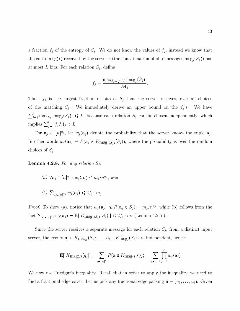
43
a fraction fj of the entropy of Sj. We do not know the values of fj, instead we know that
the entire msgpIq received by the server s (the concatenation of all ` messages msgjpSjq) has
at most L bits. For each relation Sj, define
fj maxSjrns
aj |msgjpSjq|Mj
.
Thus, fj is the largest fraction of bits of Sj that the server receives, over all choices
of the matching Sj. We immediately derive an upper bound on the fj’s. We have°`j1 maxSj
|msgjpSjq| ¤ L, because each relation Sj can be chosen independently, which
implies°`j1 fjMj ¤ L.
For aj P rnsaj , let wjpajq denote the probability that the server knows the tuple aj.
In other words wjpajq P paj P KmsgjpSjqpSjqq, where the probability is over the random
choices of Sj.
Lemma 4.2.8. For any relation Sj:
(a) @aj P rnsaj : wjpajq ¤ mjnaj , and
(b)°
ajPrnsaj wjpajq ¤ 2fj mj.
Proof. To show (a), notice that wjpajq ¤ P paj P Sjq mjnaj , while (b) follows from the
fact°
ajPrnsaj wjpajq Er|KmsgjpSjqpSjq|s ¤ 2fj mj (Lemma 4.2.5 ).
Since the server receives a separate message for each relation Sj, from a distinct input
server, the events a1 P Kmsg1pS1q, . . . , a` P Kmsg`
pS`q are independent, hence:
Er|KmsgpIqpqq|s ¸
aPrnsk
P pa P KmsgpIqpqqq ¸
aPrnsk
¹j1
wjpajq
We now use Friedgut’s inequality. Recall that in order to apply the inequality, we need to
find a fractional edge cover. Let us pick any fractional edge packing u pu1, . . . , u`q. Given

44
q, defined as in (2.1), consider the extended query, which has a new unary atom for each
variable xi:
q1px1, . . . , xkq S1px1q, . . . , S`px`q, T1px1q, . . . , Tkpxkq
For each new symbol Ti, define u1i 1°j:xiPvarspSjquj. Since u is a packing, u1i ¥ 0. Let us
define u1 pu11, . . . , u1kq.
Lemma 4.2.9. (a) The assignment pu,u1q is both a tight fractional edge packing and a tight
fractional edge cover for q1. (b)°`j1 ajuj
°ki1 u
1i k
Proof. (a) is straightforward, since for every variable xi we have u1i °j:xiPvarspSjq
uj 1.
Summing up:
k k
i1
u1i ¸
j:xiPvarspSjq
uj
k
i1
u1i `
j1
ajuj
which proves (b).
We will apply Friedgut’s inequality to the extended query q1. Set the variables wpq used
in Friedgut’s inequality as follows:
wjpajq Ppaj P KmsgjpSjqpSjqq for Sj, tuple aj P rnsaj
w1ipαq 1 for Ti, value α P rns
Recall that, for a tuple a P rnsk we use aj P rnsaj for its projection on the variables in Sj;
with some abuse, we write ai P rns for the projection on the variable xi. Assume first that
uj ¡ 0, for j 1, . . . , `. Then:
Er|Kmsgpqq|s ¸
aPrnsk
¹j1
wjpajq
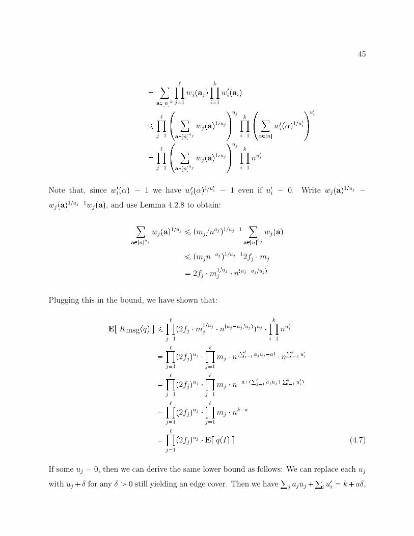
45
¸
aPrnsk
¹j1
wjpajqk¹i1
w1ipaiq
¤¹j1
¸
aPrnsaj
wjpaq1uj uj
k¹i1
¸αPrns
w1ipαq1u
1i
u1i
¹j1
¸
aPrnsaj
wjpaq1uj uj
k¹i1
nu1i
Note that, since w1ipαq 1 we have w1
ipαq1u1i 1 even if u1i 0. Write wjpaq1uj wjpaq1uj1wjpaq, and use Lemma 4.2.8 to obtain:
¸aPrnsaj
wjpaq1uj ¤ pmjnajq1uj1¸
aPrnsaj
wjpaq
¤ pmjnajq1uj12fj mj
2fj m1ujj npajajujq
Plugging this in the bound, we have shown that:
Er|Kmsgpqq|s ¤¹j1
p2fj m1ujj npajajujqquj
k¹i1
nu1i
¹j1
p2fjquj ¹j1
mj np°`
j1 ajujaq n°k
i1 u1i
¹j1
p2fjquj ¹j1
mj nap°`
j1 ajuj°k
i1 u1iq
¹j1
p2fjquj ¹j1
mj nka
¹j1
p2fjquj Er|qpIq|s (4.7)
If some uj 0, then we can derive the same lower bound as follows: We can replace each uj
with ujδ for any δ ¡ 0 still yielding an edge cover. Then we have°j ajuj
°i u
1i kaδ,

46
and hence an extra factor naδ multiplying the term n`ka in (4.7); however, we obtain the
same upper bound since, in the limit as δ approaches 0, this extra factor approaches 1.
Let fq ±`
j1p2fjquj ; the final step is to upper bound the quantity fq using the fact that°`j1 fjMj ¤ L. Recall that u °j uj, then:
fq ¹j1
p2fjquj ¹j1
fjMj
uj
uj ¹j1
2ujMj
uj
¤°`
j1 fjMj°j uj
°j uj ¹
j1
2ujMj
uj
¤
L°j uj
°j uj ¹
j1
2ujMj
uj
¹j1
2L
u Mj
uj ¹j1
pujquj
¤¹j1
2L
u Mj
uj
Here, the first inequality comes from the weighted version of the Arithmetic Mean-Geometric
Mean inequality. The last inequality holds since uj ¤ 1 for any j.
Finally, we need a lower bound on the number of bits Mj needed to represent relation
Sj. Indeed:
Proposition 4.2.10. The number of bits Mj needed to represent Sj are:
(a) If n ¥ m2j , then Mj ¤Mj2
(b) If n mj and aj ¥ 2, then Mj ¤Mj4
Proof. For the first item, we have:
Mj ¥ aj log
n
mj
¥ ajmj logpnmjq ¥ p12qajmj logpnq Mj2

47
For the second item, we have:
Mj ¥ paj 1q logpmj!q ¥ aj 1
2mj logpmjq ¥ paj 1q
2ajMj ¥Mj4
where the last inequality comes from the assumption that aj ¥ 2.
Applying the above bound on Mj, we complete the proof of Theorem 4.2.1. Recall that
our L denotes the load of an arbitrary server, which was denoted Li in the statement of the
theorem.
4.3 Proof of Equivalence
Let pkpqq be the extreme points of the convex polytope defined by the fractional edge packing
constraints in (2.2). Recall that the vertices of the polytope are feasible solutions u1,u2, . . .,
with the property that every other feasible solution u to the LP is a convex combination of
these vertices. Each vertex can be obtained by choosing m out of the k` inequalities in (2.2),
transforming them into equalities, then solving for u. Thus, it holds that |pkpqq| ¤ k`m
.
We prove here:
Theorem 4.3.1. For any vector of statistics M and number of processors p , we have:
Llower Lupper maxuPpkpqq
Lpu,M, pq
Proof. Recall that Lupper pe, where e is the optimal solution to the primal LP problem
(4.2). Consider its dual LP:
maximize¸jPr`s
µjfj f
subject to¸jPr`s
fj ¤ 1
@i P rks :¸j:iPSj
fj f ¤ 0
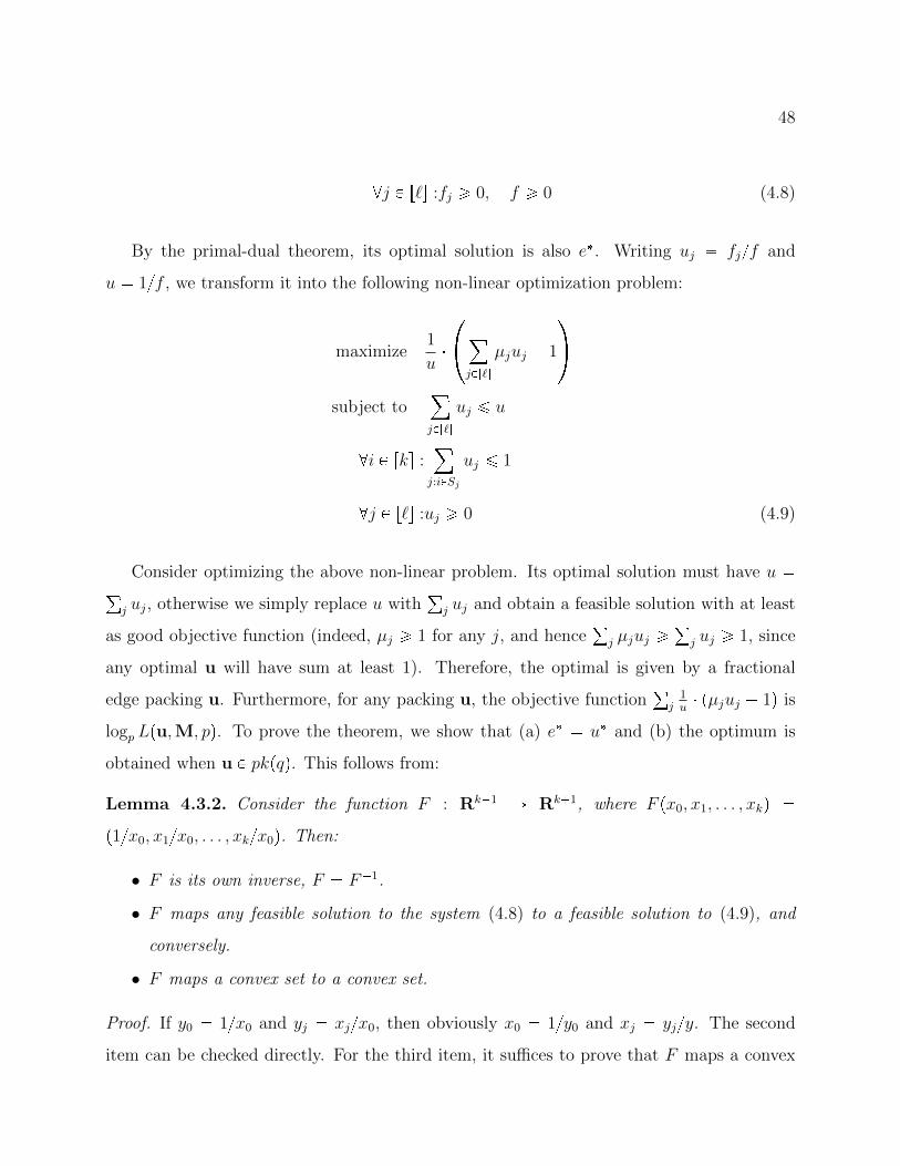
48
@j P r`s :fj ¥ 0, f ¥ 0 (4.8)
By the primal-dual theorem, its optimal solution is also e. Writing uj fjf and
u 1f , we transform it into the following non-linear optimization problem:
maximize1
u¸jPr`s
µjuj 1
subject to¸jPr`s
uj ¤ u
@i P rks :¸j:iPSj
uj ¤ 1
@j P r`s :uj ¥ 0 (4.9)
Consider optimizing the above non-linear problem. Its optimal solution must have u °j uj, otherwise we simply replace u with
°j uj and obtain a feasible solution with at least
as good objective function (indeed, µj ¥ 1 for any j, and hence°j µjuj ¥
°j uj ¥ 1, since
any optimal u will have sum at least 1). Therefore, the optimal is given by a fractional
edge packing u. Furthermore, for any packing u, the objective function°j
1u pµjuj 1q is
logp Lpu,M, pq. To prove the theorem, we show that (a) e u and (b) the optimum is
obtained when u P pkpqq. This follows from:
Lemma 4.3.2. Consider the function F : Rk1 Ñ Rk1, where F px0, x1, . . . , xkq p1x0, x1x0, . . . , xkx0q. Then:
• F is its own inverse, F F1.
• F maps any feasible solution to the system (4.8) to a feasible solution to (4.9), and
conversely.
• F maps a convex set to a convex set.
Proof. If y0 1x0 and yj xjx0, then obviously x0 1y0 and xj yjy. The second
item can be checked directly. For the third item, it suffices to prove that F maps a convex

49
combination λx λ1x1 where λ λ1 1 into a convex combination µF pxq µ1F px1q, where
µ µ1 1. Assuming x px0, x1, . . . , xkq and x1 px10, x11, . . . , x1kq, this follows by setting
µ x0pλx0 λx10q and µ1 x10pλx0 λx10q.
This completes the proof of Theorem 4.3.1.
4.4 Discussion
We present here examples and applications of the theorems proved in this section.
4.4.1 The Speedup of the HyperCube
Denote u the fractional edge packing that maximizes Lpu,M, pq (4.3). When the number
of servers increases, the load decreases at a rate of 1p1°
j uj , which we call the speedup of
the HC algorithm. We call the quantity 1°j uj the speedup exponent. Ideally, we want to
compute a query with linear speedup, which is in this case is equivalent to having°j u
j 1,
but as we have seen this holds only for very few queries.
We have seen that, when all cardinalities are equal, then the speedup exponent is 1τ,
but when the cardinalities are unequal then the speedup exponent may be better.
Example 4.4.1. Consider the triangle query
C3 S1px1, x2q, S2px2, x3q, S3px3, x1q
and assume the relation sizes are M1,M2,M3. Then, pkpC3q has five vertices, and each gives
a different value for Lpu,M, pq pMu11 Mu2
2 Mu33 pq1pu1u2u3q:
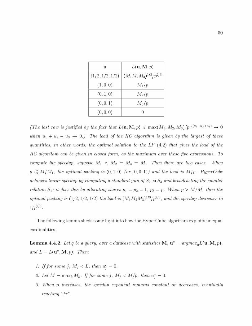
50
u Lpu,M, pqp12, 12, 12q pM1M2M3q13p23
p1, 0, 0q M1pp0, 1, 0q M2pp0, 0, 1q M3pp0, 0, 0q 0
(The last row is justified by the fact that Lpu,M, pq ¤ maxpM1,M2,M3qp1pu1u2u3q Ñ 0
when u1 u2 u3 Ñ 0.) The load of the HC algorithm is given by the largest of these
quantities, in other words, the optimal solution to the LP (4.2) that gives the load of the
HC algorithm can be given in closed form, as the maximum over these five expressions. To
compute the speedup, suppose M1 M2 M3 M . Then there are two cases. When
p ¤ MM1, the optimal packing is p0, 1, 0q (or p0, 0, 1q) and the load is Mp. HyperCube
achieves linear speedup by computing a standard join of S2 ' S3 and broadcasting the smaller
relation S1; it does this by allocating shares p1 p2 1, p3 p. When p ¡MM1 then the
optimal packing is p12, 12, 12q the load is pM1M2M3q13p23, and the speedup decreases to
1p23.
The following lemma sheds some light into how the HyperCube algorithm exploits unequal
cardinalities.
Lemma 4.4.2. Let q be a query, over a database with statistics M, u argmaxuLpu,M, pq,and L Lpu,M, pq. Then:
1. If for some j, Mj L, then uj 0.
2. Let M maxkMk. If for some j, Mj Mp, then uj 0.
3. When p increases, the speedup exponent remains constant or decreases, eventually
reaching 1τ.
51
Proof. We prove the three items of the lemma.
(1) If we modify a fractional edge packing u by setting uj 0, we still obtain a fractional
edge packing. We claim that the function fpujq Lpu,M, pq is strictly decreasing in uj on
p0,8q: the claim implies the lemma because fp0q ¡ fpujq for any uj ¡ 0. The claim follows
by noticing that fpujq ppuj logpMjbqpujcq where a, b, c are positive constants, hence f is
monotone on uj P p0,8q, and fpujq L ¡ Mj fp8q, implying that it is monotonically
decreasing.
(2) This follows immediately from the previous item by noticing that Mp ¤ L; to see the
latter, let k be such that Mk M , and let u be the packing uk 1, uj 0 for j k. Then
Mp Lpu,M, pq ¤ Lpu,M, pq L.
(3) Consider two edge packings u,u1, denote u °j uj, u1 °j u
1j, and assume u u1. Let
fppq Lpu,M, pq and gppq Lpu1,M, pq. We have fppq cp1u and gppq c1p1u1 , where
c, c1 are constants independent of p. Then fppq gppq if and only if p ¡ pcc1q1p1u1u1q,
since 1u 1u1 ¡ 0. Thus, as p increases from 1 to 8, initially we have fppq gppq,then fppq ¡ gppq, and the crossover point is pcc1q1p1u1u1q. Therefore, the value
°j u
j
can never decrease, proving the claim. To see that the speedup exponent reaches 1τ,
denote u the optimal vertex packing (maximizing°j uj) and let u be any edge packing s.t.
u °j uj τ. Then, when p1u1τ ¡ p±jMujj q1τp
±jM
ujj q1u, we have Lpu,M, pq ¡
Lpu,M, pq.
The first two items in the lemma say that, if M is the size of the largest relation, then the
only relations Sj that matter to the HC algorithm are those for which Mj ¥Mp; any smaller
relation will be broadcast by the HC algorithm. The last item says that the HC algorithm
can take advantage of unequal cardinalities and achieve speedup better than 1p1τ , e.g. by
allocating fewer shares to the smaller relations, or even broadcasting them. As p increases,
the speedup decreases until it reaches 1p1τ .
52
4.4.2 Space Exponent
Let |I| °jMj denote the size of the input database. Sometimes it is convenient to study
algorithms whose maximum load per server is given as L Op|I|p1εq, where 0 ¤ ε 1 is
a constant parameter ε called the space exponent of the algorithm. The lower bound given
by Theorem 4.2.1 can be interpreted as a lower bound on the space exponent. To see this,
consider the special case, when all relations have equal size M1 . . . M` M ; then the
load can also be written as L OpMp1εq, and, denoting u the optimal fractional edge
packing, we have°j u
j τ and Lpu,M, pq Mp1τ . Theorem 4.2.1 implies that any
algorithm with a fixed space exponent ε will report at most as many answers:
O
L
Lpu,M, pqτ
Er|qpIq|s Oppτrεp11τqsq Er|qpIq|s
Therefore, if the algorithm has a space exponent ε 1 1τ, then, as p increases, it will
return a smaller fraction of the expected number of answers. This supports the intuition
that achieving parallelism becomes harder when p increases: an algorithm with a small space
exponent may be able to compute the query correctly when p is small, but will eventually
fail, when p becomes large enough.
4.4.3 Replication Rate
Given an algorithm that computes a conjunctive query q, let Ls be the load of server s, where
s 1, . . . , p. The replication rate r of the algorithm, defined in [14], is r °ps1 Li|I|. In
other words, the replication rate computes how many times on average each input bit is
communicated. The authors in [14] discuss the tradeoff between r and the maximum load
in the case where the number of servers is not given, but can be chosen optimally. We show
next how we can apply our lower bounds to obtain a lower bound for the tradeoff between
the replication rate and the maximum load.
Corollary 4.4.3. Let q be a conjunctive query with statistics M. Any algorithm that com-

53
Conjunctive Query Share Value Lower Bound for
Exponents τpqq Space Exponent
Ckpx1, . . . , xkq k
j1 Sjpxj, xpj mod kq1q 1k, . . . , 1
kk2 1 2k
Tkpz, x1, . . . , xkq k
j1 Sjpz, xjq 1, 0, . . . , 0 1 0
Lkpx0, x1, . . . , xkq k
j1 Sjpxj1, xjq 0, 1rk2s
, 0, 1rk2s
, . . . rk2s 1 1rk2s
Bk,mpx1, . . . , xkq
Irks,|I|m SIpxIq 1k, . . . , 1
kkm 1mk
Table 4.1: Query examples: Ck cycle query, Lk linear query, Tk star query, andBk,m query with
km
relations, where each relation contains a distinct set of m out of the
k head variables. The share exponents presented are for the case where the relation sizes areequal.
putes q with maximum load L, where L ¤Mj for every Sj3 must have replication rate
r ¥ cL°jMj
maxu
¹j1
Mj
L
uj
where u ranges over all fractional edge packings of q and c maxup°j uj4q
°j uj .
Proof. Let fs be the fraction of answers returned by server s, in expectation, where I is a
randomly chosen matching database with statistics M. Let u be an edge packing for q and
cpuq p°j uj4q°
j uj ; by Theorem 4.2.1, fs ¤ L
°j uj
s
cpuq±
j Mujj
. Since we assume all answers are
returned,
1 ¤p
s1
fs p
s1
L°
j ujs
cpuq±jMujj
¤ L°
j uj1°ps1 Ls
cpuq±jMujj
L°
j uj1r|I|cpuq±jM
ujj
where we used the fact that°j uj ¥ 1 for the optimal u. The claim follows by noting that
|I| °jMj.
3if L ¡ Mj , we can send the whole relation to any processor without cost
54
Our lower bounds match the tradeoff for the queries that are discussed in [14], and
generalize the tradeoff analysis for all conjunctive queries.
In the specific case where the relation sizes are all equal to M , the above corollary tells
us that the replication rate must be r ΩppMLqτ1q. Hence, the ideal case of r op1qis achieved only when the maximum vertex cover number τ is equal to 1 (which happens if
and only if a variable occurs in every atom of the query). Another example of the replication
rate analysis is presented below:
Example 4.4.4. Consider again the triangle query C3 and assume that all sizes are equal
to M . In this case, the edge packing that maximizes the lower bound is p12, 12, 12q, and
τ 32. Thus, we obtain an ΩpaMLq bound for the replication rate for the triangle
query.
55
Chapter 5
COMPUTING JOIN QUERIES IN ONE STEP WITH SKEW
In this chapter, we focus on the effect of data skew in parallel computation. A value
in the database is skewed, and is called a heavy hitter, when its frequency exceeds some
predefined threshold. Skew for parallel joins has been studied intensively since the early
days of parallel databases, see [79]. The standard parallel join algorithm that handles skew
is the skew join [66], which consists of first detecting the heavy hitters, then treating them
differently from the others values, e.g. by partitioning tuples with heavy hitters on the other
attributes; a detailed description is in [82]. However, none of these algorithms has been
proven to be optimal in any formal sense, and to the best of our knowledge there are no
lower bounds for the communication required to compute a join in the presence of skew.
In the previous chapter, we showed tight upper and lower bounds for the load restricted
to the case where each value in the input database appears relatively few times. Here we
answer the following question: how can we compute conjunctive queries in one round under
the presence of skew? We give different answers to this question, depending on what kind of
information is available to the algorithm that computes the queries. Most of the results in
this chapter originally appear in [24, 25].
To go into more detail, let us start by presenting an example where the HC algorithm
that uses the optimal shares from (4.2) fails to work when the data has skew.
Example 5.0.5. Let qpx, y, zq S1px, zq, S2py, zq be a simple join query, where both relations
have cardinality m (and size in bits M). The optimal shares are p1 p2 1, and p3 p.
This allocation of shares corresponds to a standard parallel hash-join algorithm, where both
relations are hashed on the join variable z. When the data has no skew (in particular, when
the frequency of each value of variable z in both S1 and S2 is at most mp), the maximum

56
load is OpMpq with high probability.
However, under the presence of skew the maximum load can be as large as OpMq. Indeed,
consider the case where relation S1 is of the form tp1, 1q, p2, 1q, . . . , pm, 1qu and so is S2. In
other words, the frequency of value 1 is m in both S1 and S2. In this case, the HC algorithm
would give a maximum load of OpMq.
As we can see from the above example, the problem occurs when the input data contains
values with high frequency of occurrence, which we call outliers, or heavy hitters. In the rest
of this chapter, we will consider two different scenarios when handling data skew:
1. In the first scenario, in Section 5.1, we assume that the servers have no information on
the input data apart from the size of the relations. We study what parametrization of
the HC algorithm gives the best maximum load over all possible distributions of data.
2. In the second scenario, presented in Section 5.2, we assume that the algorithm knows
about the outliers in our data. In this case, we can do significantly better than the
no information case. We present tight algorithms for the class of star queries and the
triangle query, and a general algorithm for all conjunctive queries, which is not optimal.
5.1 The HyperCube Algorithm with Skew
We answer the following question: what are the optimal shares for the HC algorithm such that
the maximum load is minimized over all possible distributions of input data? In other words,
we limit our treatment to the HyperCube algorithm, but we consider data that can heavily
skewed, as in Example 5.0.5. Notice that the HC algorithm is oblivious to the values that
are skewed, so it cannot be modified in order to handle these cases separately. Our analysis
is based on the following lemma about hashing, which we prove in detail in Section A.2.
Lemma 5.1.1. Let RpA1, . . . , Arq be a relation of arity r with m tuples. Let p1, . . . , pr
be integers and p ±i pi. Suppose that we hash each tuple pa1, . . . , arq to the bin
ph1pa1q, . . . , hrparqq, where h1, . . . , hr are independent and perfectly random hash functions.
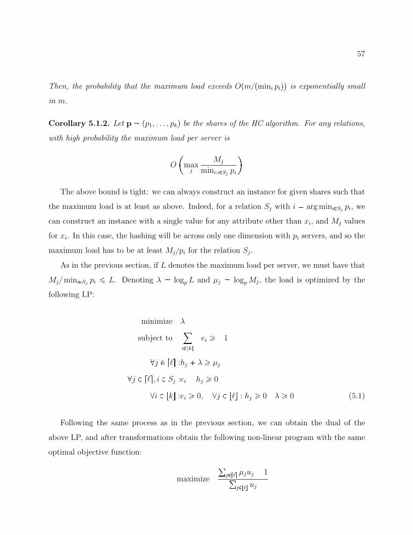
57
Then, the probability that the maximum load exceeds Opmpmini piqq is exponentially small
in m.
Corollary 5.1.2. Let p pp1, . . . , pkq be the shares of the HC algorithm. For any relations,
with high probability the maximum load per server is
O
maxj
Mj
mini:iPSjpi
The above bound is tight: we can always construct an instance for given shares such that
the maximum load is at least as above. Indeed, for a relation Sj with i arg miniPSjpi, we
can construct an instance with a single value for any attribute other than xi, and Mj values
for xi. In this case, the hashing will be across only one dimension with pi servers, and so the
maximum load has to be at least Mjpi for the relation Sj.
As in the previous section, if L denotes the maximum load per server, we must have that
MjminiPSjpi ¤ L. Denoting λ logp L and µj logpMj, the load is optimized by the
following LP:
minimize λ
subject to¸iPrks
ei ¥ 1
@j P r`s :hj λ ¥ µj
@j P r`s, i P Sj :ei hj ¥ 0
@i P rks :ei ¥ 0, @j P r`s : hj ¥ 0 λ ¥ 0 (5.1)
Following the same process as in the previous section, we can obtain the dual of the
above LP, and after transformations obtain the following non-linear program with the same
optimal objective function:
maximize
°jPr`s µjuj 1°
jPr`s uj

58
subject to @i P rks :¸j:iPSj
wij ¤ 1
@j P r`s :uj ¤¸iPSj
wij
@j P r`s :uj ¥ 0
@i P rks, j P r`s :wij ¥ 0 (5.2)
Example 5.1.3. We continue the example of the join query qpx, y, zq S1px, zq, S2py, zq,where both relations have m tuples. The optimal solution of (5.1) will give us shares px py pz 13, and maximum load of OpMp13q. Observe that this load guarantee is for
any possible data distribution, so even with a highly skewed input distribution, like the one
in Example 5.0.5, the HC algorithm will still achieve a load of OpMp13q instead of OpMq.
It is possible that some other algorithm than the HC algorithm can do better without
any skew information, but we leave this as an open question. Instead, we will next look at
how we can do much better when we are provided with information about the highly skewed
values in our data.
5.2 Skew with Information
We discuss here the case where there is additional information known about skew in the
input database. We will present a general lower bound for arbitrary conjunctive queries, and
show an algorithm that matches the bound for star queries
q S1pz, x1q, S2pz, x2q, . . . , S`pz, x`q
which are a generalization of the join query. We will also present a 1-round optimal algorithm
for the triangle query. Finally, we will describe a general algorithmic technique, which we
call the BinHC algorithm, presented first in [24], which can be used to compute arbitrary
conjunctive queries. However, there is a remaining gap between the upper and lower bounds

59
in the general case.
We first introduce some necessary notation. For each relation Sj with |Sj| mj, and
each assignment h P rns for variable z, we define its frequency as mjphq |σzhpSjq|. We
will be interested in assignments that have high frequency, which we call heavy hitters. In
order to design algorithms that take skew into account, we will assume that every input
server knows the assignments with frequency ¥ mjp for every relation Sj, along with their
frequency. Because each relation can contain at most p heavy hitters, the total number over
all relations will be Oppq. Since we are considering cases where the number of servers is
much smaller than the data, an Oppq amount of information can be easily stored in the input
server with a minimal increase of the load.
To prove the lower bound, we will make a stronger assumption about the information
available to the input servers. Given a conjunctive query q, fix a set of variables x and let
d |x| Also, let xj x X varspSjq for every relation Sj, and dj |xj|. A statistics of type
x, or x-statistics is a vector m pm1, . . . ,m`q, where mj is a function mj : rnsxj Ñ N. We
associate with m the function m : rnsx Ñ pNq`, where mphq pm1ph1q, . . . ,m`ph`qq, and hj
denotes the restriction of the tuple h to the variables in xj. We say that an instance of Sj
satisfies the statistics if for any tuple hj P rnsxj , its frequency is precisely mjphjq. When
x H, then m simply consists of ` numbers, each representing the cardinality of a relation;
thus, a x-statistics generalizes the cardinality statistics. Recall that we use upper case M pM1, . . . ,M`q to denote the same statistics expressed in bits, i.e. Mjphq ajmjphq logpnq.
5.2.1 Warmup: an Optimal Algorithm for Star Queries
For the case of the star query, we will assume that the input servers know the z-statistics;
in other words, for every assignment h P rns of variable z, we know that its frequency
in relation Sjpz, xjq is precisely mjphq. Observe that in this case the cardinality of Sj is
|Sj| °hPrnsmjphq.
The algorithm uses the same principle popular in virtually all parallel join implementa-
tions to date: identify the heavy hitters and treat them differently when distributing the
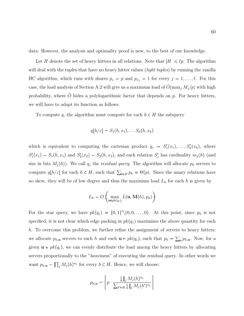
60
data. However, the analysis and optimality proof is new, to the best of our knowledge.
Let H denote the set of heavy hitters in all relations. Note that |H| ¤ `p. The algorithm
will deal with the tuples that have no heavy hitter values (light tuples) by running the vanilla
HC algorithm, which runs with shares pz p and pxj 1 for every j 1, . . . , `. For this
case, the load analysis of Section A.2 will give us a maximum load of OpmaxjMjpq with high
probability, where O hides a polylogarithmic factor that depends on p. For heavy hitters,
we will have to adapt its function as follows.
To compute q, the algorithm must compute for each h P H the subquery
qrhzs S1ph, x1q, . . . Skph, xkq
which is equivalent to computing the cartesian product qz S 11px1q, . . . , S 1kpxkq, where
S 11px1q S1ph, x1q and S 12px2q S2ph, x2q, and each relation S 1j has cardinality mjphq (and
size in bits Mjphq). We call qz the residual query. The algorithm will allocate ph servers to
compute qrhzs for each h P H, such that°hPH ph Θppq. Since the unary relations have
no skew, they will be of low degree and thus the maximum load Lh for each h is given by
Lh O
max
uPpkpqzqLpu,Mphq, phq
For the star query, we have pkpqzq t0, 1u`zp0, 0, . . . , 0q. At this point, since ph is not
specified, it is not clear which edge packing in pkpqzq maximizes the above quantity for each
h. To overcome this problem, we further refine the assignment of servers to heavy hitters:
we allocate ph,u servers to each h and each u P pkpqzq, such that ph °
u ph,u. Now, for a
given u P pkpqzq, we can evenly distribute the load among the heavy hitters by allocating
servers proportionally to the ”heaviness” of executing the residual query. In other words we
want ph,u ±
jMjphquj for every h P H. Hence, we will choose:
ph,u Sp
±jMjphquj°
h1PH
±jMjph1quj
W

61
Since rxs ¤ x 1, and |H| ¤ `p, we can compute that the total number of servers we need
is at most p` 1q |pkpqzq| p, which is Θppq. Additionally, the maximum load Lh for every
h P H will be
Lh O
max
uPpkpqzq
°hPH
±jMjphqujp
1p°
j ujq
Plugging in the values of pkpqzq, we obtain the following upper bound on the algorithm for
the heavy hitter case:
O
maxIr`s
°hPH
±jPIMjphqp
1|I|
(5.3)
Observe that the terms depend on the frequencies of the heavy hitters, and can be much
larger than the bound OpmaxjMjpq we obtain from the light hitter case. In the extreme, a
single heavy hitter h with mjphq mj for j 1, . . . , ` will demand maximum load equal to
Opp±jMjpq1`q.
5.2.2 An Optimal Algorithm for Triangle Queries
We show here how to compute the triangle query,
q Rpx, yq, Spy, zq, T pz, xq
when all relation sizes are equal to m (and have size in bits M). As with the star query, the
algorithm will deal with the tuples that have no heavy hitter values, i.e. the frequency is
less than mp13, by running the vanilla HC algorithm. For this case, we apply the standard
analysis to obtain a maximum load of OpMp23q.
Next, we show how to handle the heavy hitters. We distinguish two different cases.
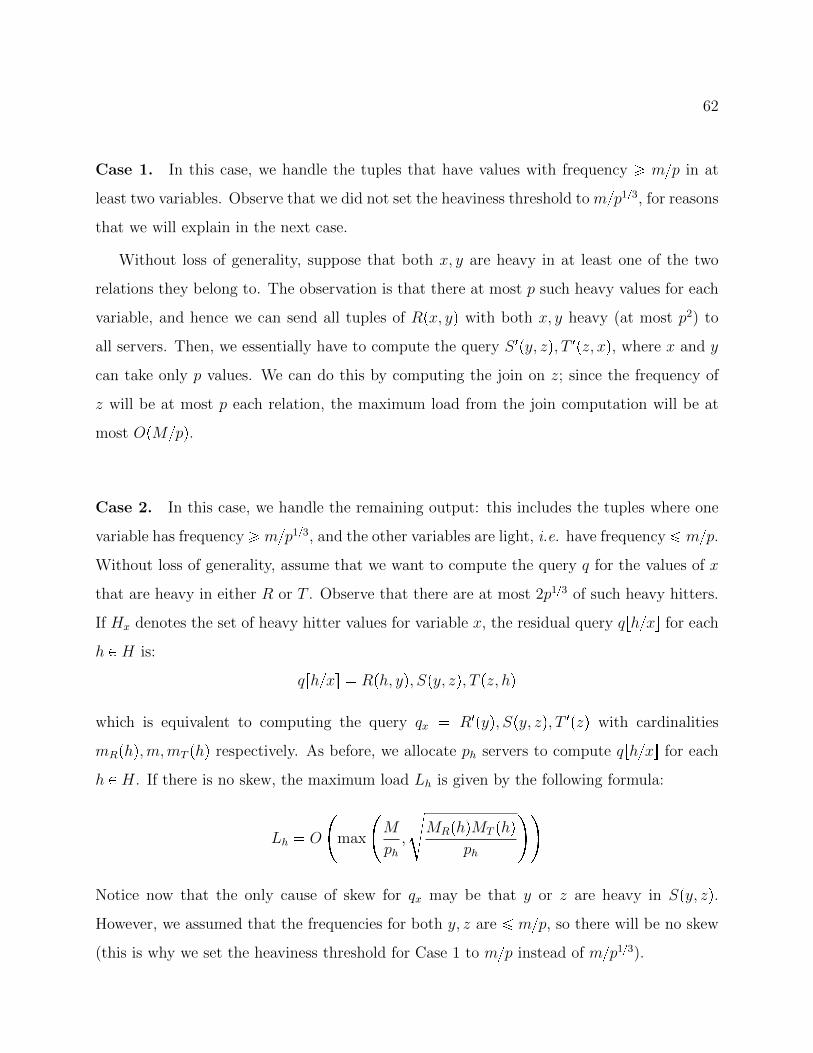
62
Case 1. In this case, we handle the tuples that have values with frequency ¥ mp in at
least two variables. Observe that we did not set the heaviness threshold to mp13, for reasons
that we will explain in the next case.
Without loss of generality, suppose that both x, y are heavy in at least one of the two
relations they belong to. The observation is that there at most p such heavy values for each
variable, and hence we can send all tuples of Rpx, yq with both x, y heavy (at most p2) to
all servers. Then, we essentially have to compute the query S 1py, zq, T 1pz, xq, where x and y
can take only p values. We can do this by computing the join on z; since the frequency of
z will be at most p each relation, the maximum load from the join computation will be at
most OpMpq.
Case 2. In this case, we handle the remaining output: this includes the tuples where one
variable has frequency ¥ mp13, and the other variables are light, i.e. have frequency ¤ mp.Without loss of generality, assume that we want to compute the query q for the values of x
that are heavy in either R or T . Observe that there are at most 2p13 of such heavy hitters.
If Hx denotes the set of heavy hitter values for variable x, the residual query qrhxs for each
h P H is:
qrhxs Rph, yq, Spy, zq, T pz, hq
which is equivalent to computing the query qx R1pyq, Spy, zq, T 1pzq with cardinalities
mRphq,m,mT phq respectively. As before, we allocate ph servers to compute qrhxs for each
h P H. If there is no skew, the maximum load Lh is given by the following formula:
Lh O
max
M
ph,
dMRphqMT phq
ph
Notice now that the only cause of skew for qx may be that y or z are heavy in Spy, zq.However, we assumed that the frequencies for both y, z are ¤ mp, so there will be no skew
(this is why we set the heaviness threshold for Case 1 to mp instead of mp13).
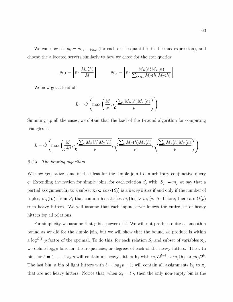
63
We can now set ph ph,1 ph,2 (for each of the quantities in the max expression), and
choose the allocated servers similarly to how we chose for the star queries:
ph,1 Rp MSphq
M
Vph,2
Rp MRphqMT phq°
hPHxMRphqMT phq
V
We now get a load of:
L O
max
M
p,
d°hMRphqMT phq
p
Summing up all the cases, we obtain that the load of the 1-round algorithm for computing
triangles is:
L O
max
M
p23,
d°hMRphqMT phq
p,
d°hMRphqMSphq
p,
d°hMSphqMT phq
p
5.2.3 The binning algorithm
We now generalize some of the ideas for the simple join to an arbitrary conjunctive query
q. Extending the notion for simple joins, for each relation Sj with |Sj| mj we say that a
partial assignment hj to a subset xj varspSjq is a heavy hitter if and only if the number of
tuples, mjphjq, from Sj that contain hj satisfies mjphjq ¡ mjp. As before, there are Oppqsuch heavy hitters. We will assume that each input server knows the entire set of heavy
hitters for all relations.
For simplicity we assume that p is a power of 2. We will not produce quite as smooth a
bound as we did for the simple join, but we will show that the bound we produce is within
a logOp1q p factor of the optimal. To do this, for each relation Sj and subset of variables xj,
we define log2 p bins for the frequencies, or degrees of each of the heavy hitters. The b-th
bin, for b 1, . . . , log2 p will contain all heavy hitters hj with mj2b1 ¥ mjphjq ¡ mj2b.The last bin, a bin of light hitters with b log2 p 1, will contain all assignments hj to xj
that are not heavy hitters. Notice that, when xj H, then the only non-empty bin is the
64
first bin, the only heavy hitter is the empty tuple hj pq, and mjphjq mj.
For a bin b on xj define βb logpp2b1q; observe that for each heavy hitter bin, there
are at most 2pβb heavy hitters in this bin, and for the last bin we have βb 1. Instead of
identifying each bin using its index b, we identify each bin by βb, called its bin exponent,
along with the index of the relation Sj for which it is defined, and the set xj varspSjq.Note that 0 β1 β2 βlog2 p1 1.
Definition 5.2.1 (Bin Combination). Let x V varspqq, and define xj xX varspSjq.A pair B pH, pβjqjq is called a bin combination if (1) βj 0 for every j where xj H,
and (2) there is some consistent assignment h to x such that for each j with xj H the
induced assignment hj to xj has bin exponent βj in relation Sj. We write CpBq for the set
of all such assignments h.
Our algorithm allocates p virtual processors to each bin combination and handles asso-
ciated inputs separately. There are Oplog pq bin choices for each relation and therefore at
most logOp1q p bin combinations in total, so at most p logOp1q p virtual processors in total.
Let Nbc be the number of possible bin combinations. As in the star join algorithm (Subsec-
tion 5.2.1), within each bin combination we partition the p servers among the heavy hitters,
using ph p1α servers for heavy hitter h (independent of h, since we have ensured complete
uniformity within a bin combination). However, we can only process pα ¤ p heavy hitters in
every bin combination: in general, we may have CpBq ¡ p, e.g. when x contains a variable
x1 in S1 and a variable x2 in S2, then there may be up to p p heavy hitters in this bin
combination.
For a bin combination B and assignment h P CpBq, write mjphq for mjphjq. For each B
we will define below a set C 1pBq CpBq with |C 1pBq| ¤ p and sets SpBqj Sj of tuples for
j P r`s that extend hj for some h P C 1pBq.The algorithm for B will compute all query answers that are joins of pSpBqj qj, by executing
the HC algorithm for a particular choice of exponents given. The share exponents for the HC
algorithm will be provided by a modification of the vertex covering primal LP (4.2), which
65
describes an algorithm that suffices for all light hitters. Recall that in this LP, µj logpMj
and λ is logp L for the load L. That LP corresponds to the bin combination BH which has
x H and all βj 0. In this case C 1pBHq CpBHq has 1 element, the empty partial
assignment. More generally, write α logp |C 1pBq|, the LP associated with our algorithm
for bin combination B is:
mininimize λ (5.4)
subject to
@j P r`s : λ¸
xiPvarspSjqxj
ei ¥ µj βj¸
iPVx
ei ¤ 1 α
@i P V x : ei ¥ 0, λ ¥ 0
Thus far, this is only fully specified for B BH since we have not defined C 1pBq for other
choices of B. We define C 1pBq inductively based on optimal solutions pλpB1q, pepB1qi qiPVx1q to
the above LP applied to bin combinations B1 with x1 x as follows. (Such solutions may
not be unique but we fix one arbitrarily for each bin combination.)
For h1 P C 1pB1q, we say that a heavy hitter hj of Sj that is an extension of h1j to xj is
overweight for B1 if there are more than Nbc mjpβj°
iPxjx1jepB1qi elements of Sj consistent
with hj. C1pBq consists of all assignments h P CpBq such that there is some j P r`s, some bin
combination B1 on set x1 x such that xx1 varspSjq, and some h1 P C 1pB1q such that h
is an extension of h1 and hj is an overweight heavy hitter of Sj for B1. The following lemma,
which is proved in the appendix, shows that α ¤ 1 and thus that the LP for B is feasible.
Lemma 5.2.2. For all bin combinations B, |C 1pBq| ¤ p.
Let AB r`s be the set of all j such that xj H. For each j P r`s AB, let SpBqj consist
of all tuples in Sj that do not contain any heavy hitter h2j of Sj that is overweight for B.
For each j P AB, and h P C 1pBq let SpBqj phq consist of all tuples in Sj that contain hj on xj

66
(with bin exponent βj) but do not contain any heavy hitter h2j of Sj that is overweight for
B and a proper extension of hj. SpBqj will be the union of all S
pBqj phq for all h P C 1pBq.
For each of the pα heavy hitter assignments h P C 1pBq the algorithm uses p1α virtual
processors to compute the join of the subinstances SpBqj phq for j P r`s. Those processors will
be allocated using the HC algorithm that assigns pepBqi shares to each variable xi P V x.
It remains to show that the load of the algorithm for B is within a logOp1q p factor of pλpBq
,
where λpBq is given by the LP for B.
Lemma 5.2.3. Let h be an assignment to x that is consistent with bin combination B. If
we hash each residual relation SpBqj phq on varspSjq xj using pe
pBqi values for each xi P
varspSjq xj, each processor receives
O
pNbc ln pqr1 mjpminpβj
°iPvarspSjqxj
epBqi ,1q
values with high probability, where r1 maxjprj |xj|q.
Proof. For j P r`s AB, SpBqj only contains tuples of Sj that are not overweight for B, which
means that for every x2j varspSjq and every heavy hitter assignment h2 to the variables
of x2j , there are at most
Nbc mjpβj°
iPx2jepBqi Nbc mjpβj
°iPx2
jxj
epBqi
elements of Sj consistent with h2. Every other assignment h2 to the variables of x2j is a
light hitter and therefore is contained in at most mjp consistent tuples of Sj. For j P AB,
we obtain the same bound, where the only difference is that we need to restrict things to
extensions of hj. This bound gives the smoothness condition on SpBqj phq necessary to apply
Lemma 4.1.2 to each relation SpBqj phq and yields the claimed result.
As a corollary, we obtain:
67
Corollary 5.2.4. Let Lmin maxjpmjpq. The maximum load of our algorithm using p
(virtual) processors for B is OppNbc ln pqrmax maxpLmin, pλqq with high probability, where
λ λpBq is the optimum of the LP for B and rmax is the maximum arity of any Sj.
Proof. There are p1α processors allocated to each h and pα such assignments h so that the
maximum load per h is also the maximum overall load. Given the presence of the Lmin
term, it suffices to show that the maximum load per h due to relation SpBqj phq is at most
pln pqk|x| maxpmjp, pλq for each j P r`s. Observe that by construction, pλ is the smallest
value such that pλ pβj°
xiPvarspSjqxjepBqi ¥ mj for all j and
°iPx e
pBqi ¤ 1 α. Lemma 5.2.3
then implies that the load due to relation SpBqj phq is at most a polylogarithmic factor times
maxpmjp,mjpβj°
xiPvarspSjqHjepBqi q
which is at most maxpmjp, pλq.
Lemma 5.2.5. Every tuple in the join of pSjqjPr`s is contained in a join of subrelations
pSpBqj qjPr`s for some bin combination B.
Proof. Observe first that every join tuple is consistent with the empty bin combination BH.
Therefore the join of pSpBHqj qjPr`s contains all join tuples that do not contain an overweight
heavy hitter hj for any relation Sj with respect to BH (and therefore contains all join tuples
that are not consistent with any heavy hitter). Now fix a join tuple t that is overweight for
BH. By definition, there is an associated relation Sj1 and x1 varspSj1q such that h1 ptx1qis an overweight heavy hitter of Sj1 for BH. Let B1 be the bin combination associated with
h1. By definition h1 P C 1pB1q. Now either t is contained in the join of pSpB1qj qjPr`s and we are
done or there is some relation Sj2 and x2 such that x2x1 varspSj2q such that h2 ptx2qhas the property that h2
j2is an overweight heavy hitter of Sj2 for B1. Again, in the latter
case, if B2 is the bin combination associated with h2 then h2 P C 1pB2q by definition and we
can repeat the previous argument for B2 instead of B1. Since the number of variables grows
at each iteration, we can repeat this at most k times before finding a first Br such that t is

68
not associated with any overweight heavy hitter for Br. In this case t will be computed in
the join of pSpBrqj qjPr`s.
We can now prove the main theorem.
Theorem 5.2.6. The algorithm that computes the joins of pSpBqj qjPr`s for every bin combina-
tion B using the HC algorithm as described above has maximum load L ¤ logOp1q pmaxB pλpBq.
Proof. There are only logOp1q p choices of B and for each choice of B, by Corollary 5.2.4, the
load with p virtual processors is logOp1q p maxpLmin, pλpBqq. To derive our claim it suffices to
show that we can remove the Lmin term. Observe that in the original LP which corresponds
to an empty bin combination B, we have λ °iPSjei ¥ µj for each j P r`s and
°i ei ¤ 1.
This implies that λ ¥ µj 1 and hence pλ ¥ mjp for each j, so pλ ¥ Lmin.
5.2.4 Lower Bound
The lower bound we present here holds for any conjunctive query, and generalizes the
lower bound in Theorem 4.2.1, which was over databases with cardinality statistics M pM1, . . . ,M`q, to databases with a fixed degree sequence. If the degree sequence is skewed,
then the new bounds can be stronger, proving that skew in the input data makes query
evaluation harder.
Let us fix statistics M of type x. We define qx as the residual query, obtained by removing
all variables x, and decreasing the arities of Sj as necessary (the new arity of relation Sj is
aj dj). Clearly, every fractional edge packing of q is also a fractional edge packing of qx,
but the converse does not hold in general. If u is a fractional edge packing of qx, we say that
u saturates a variable xi P x, if°j:xiPvarspSjq
uj ¥ 1; we say that u saturates x if it saturates
all variables in x. For a given x and u that saturates x, define
Lxpu,M, pq °
hPrnsx
±jMjphjqujqp
1°
j uj
(5.5)
69
Theorem 5.2.7. Fix statistics M of type x such that aj ¡ dj for every relation Sj. Consider
any deterministic MPC algorithm that runs in one communication round on p servers and
has maximum load L in bits. Then, for any fractional edge packing u of q that saturates x,
we must have
L ¥ minj
paj djq4aj
Lxpu,M, pq.
Note that, when x H then Lxpu,M, pq Lpu,M, pq, as defined in (4.3). However, our
theorem does not imply Theorem 4.2.1, since it does not give a lower bound on the expected
size of the algorithm output as a fraction of the expected output size.
Proof. For h P rnsx and aj P Sj, we write aj ‖ h to denote that the tuple aj from Sj matches
with h at their common variables xj, and denote pSjqh the subset of tuples aj that match
h: pSjqh taj | aj P Sj, aj ‖ hu. Let Ih denote the restriction of I to h, in other words
Ih ppS1qh, . . . , pS`qhq.We pick the domain n such that n pmaxjtmjuq2 and construct a probability space for
instances I defined by the x-statistics M as follows. For a fixed tuple h P rnsx, the restriction
Ih is a uniformly chosen instance over all matching databases with cardinality vector Mphq,which is precisely the probability space that we used in the proof of Theorem 4.3.1. In partic-
ular, for every aj P rnsxj , the probability that Sj contains aj is P paj P Sjq mjphjqnajdj .Lemma 4.2.2 immediately gives:
Er|qpIhq|s nkd¹j1
mjphjqnajdj
Let us fix some server and let msgpIq be the message the server receives on input I. As
in the previous section, let KmsgjpSjq denote the set of tuples from relation Sj known by
the server. Let wjpajq P paj P KmsgjpSjqpSjqq, where the probability is over the random
choices of Sj. This is upper bounded by P paj P Sjq:
wjpajq ¤ mjphjqnajdj , if aj ‖ h (5.6)

70
We derive a second upper bound by exploiting the fact that the server receives a limited
number of bits, in analogy with Lemma 4.2.5:
Lemma 5.2.8. Let Sj a relation with aj ¡ dj. Suppose that the size of Sj is mj ¤ n2 (or
mj n), and that the message msgjpSjq has at most L bits. Then, we have Er|KmsgjpSjq|s ¤
4Lpajdjq logpnq
.
Observe that in the case where aj dj for some relation Sj, the x-statistics fix all the
tuples of the instance for this particular relation, and hence Er|KmsgjpSjq|s mj.
Proof. We can express the entropy HpSjq as follows:
HpSjq HpmsgjpSjqq ¸
msgj
P pmsgjpSjq msgjq HpSj | msgjpSjq msgjq
¤ L¸
msgj
P pmsgjpSjq msgjq HpSj | msgjpSjq msgjq (5.7)
For every h P rnsx, let KmsgjppSjqhq denote the known tuples that belong in the restric-
tion of Sj to h. Following the proof of Lemma 4.2.5, and denoting by Mjphjq the number
of bits necessary to represent pSjqh, we have:
HpSj | msgjpSjq msgjq ¤¸
hPrnsx
1
|KmsgjppSjqhq|
2mjphjq
Mjphjq
HpSjq ¸
hPrnsx
|KmsgjppSjqhq|
2mjphjq Mjphjq
¤ HpSjq ¸
hPrnsx
|KmsgjppSjqhq|
2mjphjq mjphjqaj dj2
logpnq
HpSjq p14q |KmsgjpSjq|paj djq logpnq
where the last inequality comes from Proposition 4.2.10. Plugging this in (5.7), and solving
71
for Er|KmpSjq|s:
Er|KmsgjpSjq|s ¤ 4L
paj djq logpnq
This concludes our proof.
Let qx be the residual query, and recall that u is a fractional edge packing that saturates
x. Define the extended query qx1 to consist of qx, where we add a new atom S 1ipxiq for every
variable xi P varspqxq. Define u1i 1°j:iPSjuj. In other words, u1i is defined to be the slack
at the variable xi of the packing u. The new edge packing pu,u1q for the extended query
q1x has no more slack, hence it is both a tight fractional edge packing and a tight fractional
edge cover for qx. By adding all equalities of the tight packing we obtain:
`
j1
paj djquj kd
i1
u1i k d
We next compute how many output tuples from qpIhq will be known in expectation by
the server. Note that qpIhq qxpIhq, and thus:
Er|KmsgpqpIhqq|s Er|KmsgpqxpIhqq|s
¸a‖h
¹j1
wjpajq
¸a‖h
¹j1
wjpajqkd¹i1
w1ipaiq
¤kd¹i1
nu1i ¹j1
¸
aj‖h
wjpajq1uj uj
By writing wjpajq1uj wjpajq1uj1wjpajq for aj ‖ h, we can bound the sum in the above
72
quantity as follows:
¸aj‖h
wjpajq1uj ¤mjphjqnajdj
1uj1 ¸aj‖h
wjpajq pmjphjqndjajq1uj1Ljphq
where Ljphq °
aj‖hwjpajq. Notice that for every relation Sj, we have°
hjPrnsxj Ljphjq °
ajPrnsaj wjpajq. We can now write:
Er|KmsgpqpIhqq|s ¤ n°kd
i1 u1i
¹j1
Ljphqmjphjq1uj1npdjajqp1uj1q
uj
¹j1
Ljphquj ¹j1
mjphjquj Er|qpIhq|s (5.8)
Summing over all p servers, we obtain that the expected number of answers that can be
output for qpIhq is at most p Er|KmsgpqpIhqq|s. If some h P rnsx this number is not at least
Er|qpIhq|s, the algorithm will fail to compute qpIq. Consequently, for every h we must have
that±`
j1 Ljphjquj ¥ p1pq ±`
j1mjphjquj . Summing the inequalities for every h P rnsx:
1
p¸
hPrnsx
¹j1
mjphjquj ¤¸
hPrnsx
¹j1
Ljphjquj
¤¹j1
¸
hjPrnsxj
Ljphjq uj
by Friedgut’s inequality
¤¹j1
4L
paj djq logpnquj
by Lemma 5.2.8
Solving for L and using the fact that Mj ajmj logpnq, we obtain that for any edge packing
u that saturates x,
L ¥
minj
aj dj4aj
°
hPrnsx
±jMjphjqujp
1°
j uj

73
which concludes the proof.
To see how Theorem 5.2.7 applies to the star query, we assume that the input servers
know z-statistics M; in other words, for every assignment h P rns of variable z, we know
that its frequency in relation Sj is mjphq. Then, for any edge packing u that saturates z, we
obtain a lower bound of
L ¥ p18q °
hPrns
±jMjphqujp
1°
j uj
Observe that the set of edge packings that saturate z and maximize the above quantity is
t0, 1u`zp0, . . . , 0q. Hence, we obtain a lower bound
L ¥ p18q maxIr`s
°hPrns
±jPIMjphqp
1|I|
A similar argument proves the optimality for the triangle query C3.

74
Chapter 6
COMPUTING JOIN QUERIES IN MULTIPLE ROUNDS
In this chapter, we analyze the computation of conjunctive queries in the MPC model for
algorithms with multiple rounds. We show that there exists a tradeoff between the number
of rounds and the load when computing queries, at least for the case where the input data
has no skew: using more rounds, and hence more synchronization, it is possible to achieve a
better load per round.
We mainly focus on the following question: given a query q over input data without skew,
what is the optimal load to compute q in r rounds, where r ¥ 2? In Section 6.1, we provide
both upper and lower bounds for the case of matching databases. In order to prove lower
bounds for the case of multiple rounds, we restrict to the tuple-based MPC model, where it
is easier to analyze how communication is performed. A surprising consequence of our lower
bounds is that computing connected components in a graph of size M cannot be done in a
constant number of rounds with load less than M .
In Section 6.2, we briefly explore the computation of conjunctive queries in multiple
rounds for any input data. In particular, we present an algorithm for computing the triangle
query in 2 rounds with worst-case load that is better than the load that can be achieved in
a single round.
6.1 Input Data without Skew
To present and analyze the behavior of multi-round algorithms, we restrict both the structure
of the input and the type of computation in the MPC model. In particular, our multi-round
algorithms will process only queries where the relations are of equal size and the data has no
skew. Additionally, our lower bounds are proven for a restricted version of the MPC model,

75
called the the tuple-based MPC model, which limits the way communication is performed.
6.1.1 An Algorithm for Multiple Rounds
In Chapter 4, we showed that in the case where all relations have size equal to M and
are matching databases (i.e. the degree of any value is exactly one), we can compute a
conjunctive query q in one round with maximum load
L OpMp1τpqqq
where τpqq denotes the fractional vertex covering number of q. Hence, for any ε ¥ 0, a
conjunctive query q with τpqq ¤ 1p1εq can be computed in one round in the MPC model
with load L OpMp1εq; recall from Section 4.4 that we call the parameter ε the space
exponent.
We define now the class of queries Γrε using induction on r. For r 1, we define
Γ1ε tq | τpqq ¤ 1p1 εqu
For r ¡ 1, we define Γrε to be the set of all conjunctive queries q constructed as fol-
lows. Let q1, . . . , qm P Γr1ε be m queries, and let q0 P Γ1
ε be a query over a different
vocabulary V1, . . . , Vm, such that |varspqjq| aritypVjq for all j P rms. Then, the query
q q0rq1V1, . . . , qmVms, obtained by substituting each view Vj in q0 with its definition qj,
is in Γrε. In other words, Γrε consists of queries that have a query plan of depth r, where each
operator is a query computable in one step with maximum load OpMp1εq. The following
proposition is now straightforward.
Proposition 6.1.1. Every conjunctive query q P Γrε with input a matching database where
each relation has size M can be computed by an MPC algorithm in r rounds with maximum
load L OpMp1εq.
We next present two examples that provide some intuition on the structure of the queries
76
in the class Γrε.
Example 6.1.2. Consider the query Lk in Table 4.1 with k 16; we can construct a query
plan of depth r 2 and load L OpMp12q (with space exponent ε 12). The first step
computes in parallel four queries, v1 S1, S2, S3, S4, . . . , v4 S13, S14, S15, S16. Each query
is isomorphic to L4, therefore τpq1q τpq4q 2 and thus each can be computed in
one step with load L OpMp1τpq1qq OpMp12q. The second step computes the query
q0 V1, V2, V3, V4, which is also isomorphic to L4.
We can generalize the above approach for any query Lk. For any ε ¥ 0, let kε be the
largest integer such that Lkε P Γε1. In other words, τpLkεq ¤ 1p1 εq and so we choose
kε 2t1p1 εqu. Then, for any k ¥ kε, Lk can be computed using Lkε as a building
block at each round: the plan will have a depth of rlogkεpkqs and will achieve a load of
L OpMp1εq.
Example 6.1.3. Consider the query SPk k
i1Ripz, xiq, Sipxi, yiq. Since τpSPkq k,
the one round algorithm can achieve a load of OpMp1kq.However, we can construct a query plan of depth 2 for SPk with load OpMpq, by com-
puting the joins qi Ripz, xiq, Sipxi, yiq in the first round and in the second round joining
all qi on the common variable z.
We next present an upper bound on the number of rounds needed to compute any query
if we want to achieve a given load L OpMp1εq; in other words, we ask what is the
minimum number of rounds for which we can achieve a space exponent ε.
Let radpqq minu maxv dpu, vq denote the radius of a query q, where dpu, vq denotes
the distance between two nodes in the hypergraph of q. For example, radpLkq rk2s and
radpCkq tk2u.
Lemma 6.1.4. Fix ε ¥ 0, let kε 2t1p1 εqu, and let q be any connected query. Define
rpqq
$'&'%
rlogkεpradpqqqs 1 if q is tree-like,
tlogkεpradpqqqu 2 otherwise.
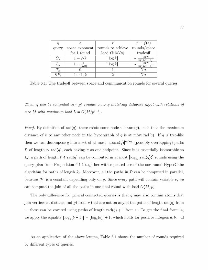
77
q ε r r fpεqquery space exponent rounds to achieve rounds/space
for 1 round load OpMpq tradeoff
Ck 1 2k rlog ks log klogp2p1εqq
Lk 1 1rk2s
rlog ks log klogp2p1εqq
Tk 0 1 NASPk 1 1k 2 NA
Table 6.1: The tradeoff between space and communication rounds for several queries.
Then, q can be computed in rpqq rounds on any matching database input with relations of
size M with maximum load L OpMp1εq.
Proof. By definition of radpqq, there exists some node v P varspqq, such that the maximum
distance of v to any other node in the hypergraph of q is at most radpqq. If q is tree-like
then we can decompose q into a set of at most |atomspqq|radpqq (possibly overlapping) paths
P of length ¤ radpqq, each having v as one endpoint. Since it is essentially isomorphic to
L`, a path of length ` ¤ radpqq can be computed in at most rlogkεpradpqqqs rounds using the
query plan from Proposition 6.1.1 together with repeated use of the one-round HyperCube
algorithm for paths of length kε. Moreover, all the paths in P can be computed in parallel,
because |P | is a constant depending only on q. Since every path will contain variable v, we
can compute the join of all the paths in one final round with load OpMpq.The only difference for general connected queries is that q may also contain atoms that
join vertices at distance radpqq from v that are not on any of the paths of length radpqq from
v: these can be covered using paths of length radpqq 1 from v. To get the final formula,
we apply the equality rlogapb 1qs tlogapbqu 1, which holds for positive integers a, b.
As an application of the above lemma, Table 6.1 shows the number of rounds required
by different types of queries.
78
6.1.2 Lower Bounds for Multiple Rounds
We present here a general lower bound for connected conjunctive queries in the tuple-based
MPC model.
We first introduce a combinatorial object associated with every query q, called the pε, rq-plan, which is central to the construction of the multi-round lower bound. We next define
this notion, and also discuss how we can construct such plans for various classes of queries.
Given a query q and a set M atomspqq, recall that qM is the query that results from
contracting the edges M in the hypergraph of q. Also, we define M atomspqqzM .
Definition 6.1.5. Let q be a connected conjunctive query. A set M atomspqq is ε-good
for q if it satisfies the following two properties:
1. Every connected subquery of q that is in Γ1ε contains at most one atom in M .
2. χpMq 0 (and thus χpqMq χpqq by Lemma 2.1.4).
For ε P r0, 1q and integer r ¥ 0, an pε, rq-plan M is a sequence M1, . . . ,Mr, with M0 atomspqq M1 Mr such that (a) for j 0, . . . , r 1, Mj1 is ε-good for qM j, and
(b) qM r R Γ1ε.
We provide some intuition about the above definition with the next two lemmas, which
shows how we can obtain such a plan for the query Lk and Ck respectively.
Lemma 6.1.6. The query Lk admits an pε, rlogkεpkqs 2q-plan for any integer k ¡ kε 2t1p1 εqu.
Proof. We will prove using induction that for every integer r ¥ 0, if k ¥ kr1ε 1 then Lk
admits an pε, rq-plan. This proves the lemma, because then for a given k the smallest integer
r we can choose for the plan is r tlogkεpk 1qu 1 rlogkεpkqs 2. For the base case
r 0, we have that k ¥ kε 1, and observe that LkM0 Lk R Γ1ε.
For the induction step, let k0 ¥ kr1ε 1; then from the inductive hypothesis for every
k ¥ krε 1 the query Lk has an pε, r 1q-plan. Define M to be the set of atoms where we

79
include every kε-th atom Lk0 , starting with S1; in other words, M tS1, Skε1, S2kε1, . . .u.Observe now that Lk0M S1px0, x1q, Skε1px1, xkε1q, S2kε1pxkε1, x2kε1q, . . ., which is
isomorphic to Lrk0kεs.
We will show first that M is ε-good for Lk0 . Indeed, χpLk0Mq χpLrk0kεq χpLk0qand thus property (2) is satisfied. Additionally, recall that Γ1
ε consists of queries for which
τpqq ¤ 1p1εq; thus the connected subqueries of Lk0 that are in Γ1ε are precisely queries of
the form Sjpxj1, xjq, Sj1pxj, xj1q, . . . , Sjk1pxjk2, xjk1q, where k ¤ kε. By choosing
M to contain every kε-atom, no such subquery in Γ1ε will contain more than one atom from
M and thus property (1) is satisfied as well.
Finally, we have that rk0kεs ¥ rkrε 1kεs krε 1 and thus from the inductive hy-
pothesis the query Lk0M admits an pε, r 1q-plan. By definition, this implies a sequence
M1, . . . ,Mr1; the extended sequence M,M1, . . . ,Mr1 will now be an pε, rq-plan for Lk0 .
Lemma 6.1.7. The query Ck admits an pε, tlogkεpkpmε 1qquq-plan, for every integer k ¡mε t2p1 εqu.
Proof. The proof is similar to the proof for the query Lk, since we can observe that any set
M of atoms that are (at least) kε apart along any cycle Ck is a ε-good set for Ck and further
CkM is isomorphic to Ctkkεu. The only difference is that the base case for r 0 is that
k ¥ mε 1. Thus, the inductive step is that for every integer r ¥ 0, if k ¥ krεpmε 1q then
Ck admits an pε, rq-plan.
The above examples of queries show how we can construct pε, rq-plans. We next present
the main theorem of this section, which tells us how we can use such plans to obtain lower
bounds on the number of communication rounds needed to compute a conjunctive query.
Theorem 6.1.8 (Lower Bound for Multiple Rounds). Let q be a conjunctive query that
admits an pε, rq-plan. For every randomized algorithm in the tuple-based MPC model that
computes q in r 1 rounds and with load L ¤ cMp1ε for a sufficiently small constant c,
there exists a (matching) instance I with relations of size M where the algorithm fails to
compute q with probability Ωp1q.
80
The constant c in the above theorem depends on the query q and the parameter ε. To
state the precise expression the constant c, we need some additional definitions.
Definition 6.1.9. Let q be a conjunctive query and M be an pε, rq-plan for q. We de-
fine τpMq to be the minimum of τpqM rq and τpq1q, where q1 ranges over all connected
subqueries of qM j1, j P rrs, such that q1 R Γ1ε.
Proposition 6.1.10. Let q be a conjunctive query and M be an pε, rq-plan for q. Then,
τpMq ¡ 1p1 εq.
Proof. For every q1 R Γ1ε, we have by definition that τpq1q ¡ 1p1 εq. Additionally, by the
definition of an pε, rq-plan, we have that τpqM rq ¡ 1p1 εq.
Further, for a given query q let us define the following sets:
Cpqq tq1 | q1 is a connected subquery of quCεpqq tq1 | q1 R Γ1
ε, q1 is a connected subquery of qu
Sεpqq tq1 | q1 R Γ1ε, q
1 is a minimal connected subquery of qu.
and let
βpq,Mq
1
τpqM rq
τpMq
r
k1
¸q1PSεpqMk1q
1
τpq1qτpMq
We can now present the precise statement.
Theorem 6.1.11. If q has an pε, rq-plan M then any deterministic tuple-based MPC algo-
rithm running in r 1 rounds with maximum load L reports at most
βpq,Mq pr 1qL
M
τpMq
p Er|qpIq|s
correct answers in expectation over a uniformly at random chosen matching database I where
each relation has size M .

81
The above theorem implies Theorem 6.1.8 by following the same proof as in Theo-
rem 4.2.3. Indeed, for L ¤ cMp1ε we obtain that the output tuples will be at most
f Er|qpIq|s, where f βpq,Mq ppr 1qcqτpMq. If we choose the constant c such that
f 19, we can apply Lemma 4.2.4 to show that for any randomized algorithm we can find
an instance I where it will fail to produce the output with probability Ωp1q.In the rest of this section, we present the proof of Theorem 6.1.11. Let A be an algorithm
that computes q in r 1 rounds. The intuition is as follows. Consider an ε-good set M ;
then any matching database i consists of two parts, i piM , iMq,1 where iM are the relations
for atoms in M , and iM are all the other relations. We show that, for a fixed instance iM ,
the algorithm can be used to compute qMpiMq in r 1 rounds; however, the first round
is almost useless, because the algorithm can discover only a tiny number of join tuples with
two or more atoms Sj P M (since every subquery q1 of q that has two atoms in M is not in
Γ1ε). This shows that the algorithm can compute most of the answers in qMpiMq in only r
rounds, and we repeat the argument until a one-round algorithm remains.
To formalize this intuition, we need some notation. For two relations A,B we write AB,
called the semijoin, to denote the set of tuples in A for which there is a tuple in B that has
equal values on their common variables. We also write ABB, called the antijoin, to denote
the set of tuples in A for which no tuple in B has equal values on their common variables.
Let A be a deterministic algorithm with r 1 rounds, k P rr 1s a round number, s a
server, and q1 a subquery of q. We define:
KA,k,smsgpq1q ta1 P rnsvarspq1q | @ matching database i,msg¤ks pA, iq msg ñ a1 P q1piqu
KA,kmsgpq1q
p¤s1
KA,k,smsgs
pq1q
Using the above notation, KA,k,smsg¤k
s pA,iqpq1q and KA,kmsg¤kpA,iqpq1q denote the set of join tuples
from q1 known at round k by server s, and by all servers, respectively, on input i. Further,
1We will use i to denote a fixed matching instance, as opposed to I that denotes a random instance.

82
Apiq KA,r1
msg¤r1pA,iqpqq is w.l.o.g. the final answer of the algorithm A on input i. Finally,
let us define
JA,qpiq ¤
q1PCpqq
KA,1msg¤1pA,iqpq1q
JA,qε piq
¤q1PCεpqq
KA,1msg¤1pA,iqpq1q
JA,qε piq is precisely the set of join tuples known after the first round, but restricted to those
that correspond to subqueries that are not computable in one round; thus, the number of
tuples in JA,qε piq will be small.
We can now state the two lemmas we need as building blocks to prove Theorem 6.1.11.
Lemma 6.1.12. Let q be a query, and M be any ε-good set for q. If A is an algorithm with
r 1 rounds for q, then for any matching database iM over the atoms of M , there exists
an algorithm A1 with r rounds for qM using the same number of processors and the same
total number of bits of communication received per processor such that, for every matching
database iM defined over the atoms of M :
|ApiM , iMq| ¤ |qpiM , iMq JA,qε piM , iMq| |A1piMq|.
In other words, the algorithm returns no more answers than the (very few) tuples in
JA,qε , plus what another algorithm A1 that we define next computes for qM using one fewer
round.
Proof. We call qM the contracted query. While the original query q takes as input the
complete database i piM , iMq, the input to the contracted query is only iM . Observe also
that for different matching databases iM , the lemma produces different algorithms A1. We
fix now a matching database iM .
The construction of A1 is based on the following two constructions, which we call con-
traction and retraction.
83
Contraction. We first show how to use the algorithm A to derive an algorithm Ac for qMthat uses the same number of rounds as A.
For each connected component qc of M , we choose a representative variable zc P varspqcq.The query answer qcpiMq is a matching instance, since qc is tree-like (because χpMq 0).
Denote mσ tσx | x P varspqqu, where, for every variable x P varspqq, σx : rns Ñ rns is the
following permutation. If x R varspMq, then σx is defined as the identity, i.e. σxpaq a for
every a P rns. Otherwise, if qc is the unique connected component such that x P varspqcqand a P qcpiMq is the unique tuple such that ax a, we define σxpaq azc . In other words,
we think of mσ as permuting the domain of each variable x P varspqq. Observe that mσ is
known to all servers, since iM is a fixed instance.
It holds that mσpqpiqq qpmσpiqq, and mσpiMq idM , where idM is the identity
matching database (where each relation in M is tp1, 1, . . .q, p2, 2, . . .q, . . .u). Therefore,2
qMpiMq mσ1pΠvarspqMqpqpmσpiMq, idMqqq
Using the above equation, we can now define the algorithm Ac that computes the query
qMpiMq. First, each input server for Sj P M replaces Sj with mσpSjq. Second, we run A
unchanged, substituting all relations Sj P M with the identity. Finally, we apply mσ1 to
the answers and return the output. Hence, we have:
AcpiMq mσ1pΠvarspqMqpApmσpiMq, idMqqq (6.1)
Retraction. Next, we transform Ac into a new algorithm Ar, called the retraction of Ac,
that takes as input iM as follows.
• In round 1, each input server for Sj sends (in addition to the messages sent by Ac)
2We assume varspqMq varspqq; for that, when we contract a set of nodes of the hypergraph, we replacethem with one of the nodes in the set.
84
every tuple in aj P Sj to all servers s that eventually receive aj. In other words,
the input server sends t to every s for which there exists k P rr 1s such that aj PKAc,k,s
msg¤ks pAc,iM q
pSjq. This is possible because of the restrictions in the tuple-based MPC
model: all destinations of aj depend only on Sj, and hence can be computed by the
input server. Note that this does not increase the total number of bits received by any
processor, though it does mean that more communication will be performed during the
first round.
• In round 2, Ar sends no tuples.
• In rounds k ¥ 3, Ar sends a join tuple t from server s to server s1 if server s knows t
at round k, and also algorithm Ac sends t from s to s1 at round k.
Observe first that the algorithm Ar is correct, in the sense that the output ArpiMq will
be a subset of qMpiMq. We now need to quantify how many tuples Ar misses compared to
the contracted algorithm Ac. Let QM tq1 | q1 subquery of qM, |q1| ¥ 2u, and define:
JAc
piMq ¤
q1PQM
KAc,1
msg1pAc,iqpq1q.
The set JAc
piMq is exactly the set of non-atomic tuples known by Ac right after round 1:
these are also the tuples that the new algorithm Ar will choose not to send during round 2.
Lemma 6.1.13. pAcpiMqB JAc
piMqq ArpiMq
Proof. We will prove the statement by induction on the number of rounds: for any subquery
q1 of qM , if server s knows t P pq1piMqB JAc
piMqq at round k for algorithm Ac, then server
s knows t at round k for algorithm Ar as well.
For the induction base, in round 1 we have by construction that KAc,1,s
msg1spAc,iM q
pSjq KAr,1,s
msg1spAr,iM q
pSjq for every Sj P M , and thus any tuple t (join or atomic) that is known by
server s for algorithm Ac will be also known for algorithm Ar.
Consider now some round k 1 and a tuple t P pq1piMq B JAc
piMqq known by server s
for algorithm Ac. If q1 is a single relation, the statement is correct since by construction all
85
atomic tuples are known at round 1 for algorithm Ar. Otherwise q1 P QM . Let t1, . . . , tm
be the subtuples at server s from which tuple t is constructed, where tj P qjpiMq for every
j 1, . . . ,m. Observe that tj P pqjpiMq B JAc
piMqq. Thus, if ti was known at round k by
some server s1 for algorithm Ac, by the induction hypothesis it would be known by server s1
for algorithm Ar as well, and thus it would have been communicated to server s at round
k 1.
From the above lemma it follows that:
AcpiMq ArpiMq Y pqMpiMq JAc
piMqq (6.2)
Additionally, by the definition of ε-goodness, if a subquery q1 of q has two atoms in M , then
q1 R Γ1ε. Hence, we also have:
JAc
piMq mσ1pΠvarspqMqpJA,qε pmσpiqqqq (6.3)
SinceAr send no information during the second round, we can compress it to an algorithm
A1 that uses only r rounds. Finally, since M is ε-good, we have χpqMq χpqq and thus
|AcpiMq| |ApiM , iMq|. Combining everything together:
|ApiM , iMq| |AcpiMq|¤ |ArpiMq| |pqMpiMq JAc
piMqq|¤ |A1piMq| |pqMpiMq mσ1pΠvarspqMqpJA,q
ε pmσpiqqqq|¤ |A1piMq| |ΠvarspqMqpqpiq JA,q
ε piqq|¤ A1piMq| |qpiq JA,q
ε piq|
This concludes the proof.
Lemma 6.1.14. Let q be a conjunctive query and q1 a subquery of q. Let B be any algorithm
that outputs a subset of answers to q1 (i.e. for every database i, Bpiq q1piq). Let I be a
86
uniformly at random chosen matching database for q, and I 1 Iatomspq1q its restriction over
the atoms in q1.
If Er|BpI 1q|s ¤ γ Er|q1pI 1q|s, then Er|qpIq BpI 1q|s ¤ γ Er|qpIq|s.
Proof. Let y varspq1q and d |y|. By symmetry, the quantity Er|σyapqpIqq|s is indepen-
dent of a, and therefore equals Er|qpIq|snd. Notice that by construction σyapBpi1qq tau.We now have:
Er|qpIq BpI 1q|s ¸
aPrnsd
Er|σyapqpIqq σyapBpI 1qq|s
¸
aPrnsd
Er|σyapqpIqq|s P pa P BpI 1qq
Er|qpIq|snd ¸aPrnsd
Ppa P BpI 1qq
Er|qpIq|s Er|BpI 1q|snd
¤ Er|qpIq|s pγ Er|q1pI 1q|sqnd
¤ γ Er|qpIq|s
where the last inequality follows from the fact that Er|q1pI 1q|s ¤ nd (since for every database
i1, we have |q1pi1q| ¤ nd).
Proof of Theorem 6.1.11. Given an pε, rq-plan atomspqq M0 M1 . . . Mr, we define
Mk Mk Mk1, for k ¥ 1. Let A be an algorithm for q that uses pr 1q rounds.
We start by applying Lemma 6.1.12 for algorithm A and the ε-good set M1. Then, for
every matching database iM1 iM1
, there exists an algorithm Ap1qiM1
for qM1 that runs in r
rounds such that for every matching database iM1 we have:
|Apiq| ¤ |qpiq JA,qε piq| |Ap1q
iM1
piM1q|
We can iteratively apply the same argument. For k 1, . . . , r 1, let us denote Bk ApkqiMk
87
the inductively defined algorithm for query qMk, and consider the ε-good set Mk1. Then,
for every matching database iMk1there exists an algorithm Bk1 Apk1q
iMk1
for qMk1 such
that for every matching database iMk1, we have:
|BkpiMkq| ¤ |qMkpiMk
q JBk,qMkε piMk
q| |Bk1piMk1q|
We can now combine all the above inequalities for k 0, . . . , r 1 to obtain:
|Apiq| ¤ |qpiq JA,qε piMr , iM1
, . . . , iMrq|
|qM1piM1q JB1,qM1ε piMr , iM2
, . . . , iMrq|
. . . |qM r1piMr1q JBr1,qMr1
ε piMr , iMrq|
|BrpiMrq| (6.4)
We now take the expectation of (6.4) over a uniformly chosen matching database I and
upper bound each of the resulting terms. Observe first that for all k 0, . . . , r we have
χpqMkq χpqq, and hence, by Lemma 4.2.2, we have Er|qpIq|s Er|pqMkqpIMkq|s.
We start by analyzing the last term of the equation, which is the expected output of an
algorithm Br that uses one round to compute qM r. By the definition of τpMq, we have
τpqM rq ¥ τpMq. Since the number of bits received by each processor in the first round
of algorithm Br is at most r 1 times the bound for the original algorithm A, we can apply
Theorem 4.2.1 to obtain that:
ErBrpIMrqs ¤ p
pr 1qLτpqM rqM
τpqMrq
Er|pqM rqpIMrq|
¤ p
pr 1qLτpqM rqM
τpMq
Er|qpIq||
We next bound the remaining terms. Note that IMk1 pIMr , IMk
, . . . , IMrq and consider

88
the expected number of tuples in J JBk1,qMk1ε pIMk1
q. The algorithm Bk1 Apk1qIMk1
itself depends on the choice of IMk1; still, we show that J has a small number of tuples. Every
subquery q1 of qMk1 that is not in Γ1ε (and hence contributes to J) has τpq1q ¥ τpMq.
For each fixing IMk1 iMk1
, the expected number of tuples produced for subquery q1 by
Bq1 , where Bq1 is the portion of the first round of Apk1qiMk1
that produces tuples for q1, satisfies
Er|Bq1pIMk1q|s ¤ γpq1q Er|q1pIMk1
q|s, where
γpq1q p
pr 1qLτpq1qM
τpMq
since each processor in a round of Apk1qiMk1
(and hence Bq1) receives at most r 1 times the
communication bound for a round of A. We now apply Lemma 6.1.14 to derive
Er|qpIq Bq1pIMk1q|s Er|pqMk1qpIMk1
q Bq1pIMk1q|s
¤ γpq1q Er|pqMk1qpIMk1q|s
γpq1q Er|qpIq|s.
Averaging over all choices of IMk1 iMk1
and summing over the number of different
queries q1 P SpqMk1q, where we recall that SεpqMk1q is the set of all minimal connected
subqueries q1 of qMk1 that are not in Γ1ε, we obtain
Er|qpIqJAk1,qMk1ε pIMk1
q|s ¤¸
q1PSεpqMk1q
γpq1q Er|qpIq|s
Combining the bounds obtained for the r 1 terms in (6.4), we conclude that Er|ApIq|s is
at most
1
τpqM rq
τpMq
r
k1
¸q1PSεpqMk1q
1
τpq1qτpMq
pr 1qL
M
τpMq
p Er|qpIq|s
89
βpq,Mq pr 1qL
M
τpMq
p Er|qpIq|s
which proves Theorem 6.1.11.
6.1.3 Application of the Lower Bound
We show now how to apply Theorem 6.1.8 to obtain lower bounds for several query classes,
and compare the lower bounds with the upper bounds.
The first class is the queries Lk, where the following corollary is a straightforward appli-
cation of Theorem 6.1.8 and Lemma 6.1.6.
Corollary 6.1.15. Any tuple-based MPC algorithm that computes the query Lk (on matching
databases) with load L OpMp1εq requires at least rlogkε ks rounds of computation.
Observe that this gives a tight lower bound for Lk, since in the previous section we showed
that there exists a query plan with depth rlogkε ks and load OpMp1εq.Second, we give a lower bound for tree-like queries, and for that we use a simple obser-
vation:
Proposition 6.1.16. Let q be a tree-like query, and q1 be any connected subquery of q. Any
algorithm that computes q1 with load L needs at least as many rounds to compute q with the
same load.
Proof. Given any tuple-based MPC algorithm A for computing q in r rounds with maximum
load L, we construct a tuple-based MPC algorithm A1 that computes q1 in r rounds with at
most load L. A1 will interpret each instance over q1 as part of an instance for q by using the
relations in q1 and using the identity permutation (Sj tp1, 1, . . .q, p2, 2, . . .q, . . .u) for each
relation in qzq1. Then, A1 runs exactly as A for r rounds; after the final round, A1 projects
out for every tuple all the variables not in q1. The correctness of A1 follows from the fact
that q is tree-like.
90
Define diampqq, the diameter of a query q, to be the longest distance between any two
nodes in the hypergraph of q. In general, radpqq ¤ diampqq ¤ 2 radpqq. For example,
radpLkq tk2u, diampLkq k and radpCkq diampCkq tk2u.
Corollary 6.1.17. Any tuple-based MPC algorithm that computes a tree-like query q (on
matching databases) with load L OpMp1εq needs at least rlogkεpdiampqqqs rounds.
Proof. Let q1 be the subquery of q that corresponds to the diameter of q. Notice that q1 is a
connected query, and moreover, it behaves exactly like Ldiampqq. Hence, by Corollary 6.1.15
any algorithm needs at least rlogkεpdiampqqqs to compute q1. By applying Proposition 6.1.16,
we have that q needs at least that many rounds as well.
Let us compare the lower bound rlow rlogkεpdiampqqqs and the upper bound rup rlogkεpradpqqqs 1 from Lemma 6.1.4. Since diampqq ¤ 2radpqq, we have that rlow ¤ rup.
Additionally, radpqq ¤ diampqq implies rup ¤ rlow 1. Thus, the gap between the lower
bound and the upper bound on the number of rounds is at most 1 for tree-like queries.
When ε 12, these bounds are matching, since kε 2 and 2radpqq 1 ¤ diampqq for
tree-like queries.
Third, we study one instance of a non tree-like query, namely the cycle query Ck. The
lemma is a direct application of Lemma 6.1.7.
Lemma 6.1.18. Any tuple-based MPC algorithm that computes the query Ck (on matching
databases) with load L OpMp1εq requires at least tlogkεpkpmε 1qqu 2 rounds, where
mε t2p1 εqu.
For cycle queries we also have a gap of at most 1 between this lower bound and the upper
bound in Lemma 6.1.4.
Example 6.1.19. Let ε 0 and consider two queries, C5 and C6. In this case, we have
kε mε 2, and radpC5q radpC6q 2.
For query C6, the lower bound is then tlog2p63qu 2 3 rounds, while the upper bound
is rlog2p3qs 1 3 rounds. Hence, in the case of C6 we have tight upper and lower bounds.
91
For query C5, the upper bound is again rlog2p3qs1 3 rounds, but the lower bound becomes
tlog2p53qu 2 2 rounds. The exact number of rounds necessary to compute C5 is thus
open.
Finally, we show how to apply Corollary 6.1.15 to show that transitive closure requires
many rounds. In particular, we consider the problem Connected-Components, for which,
given an undirected graph G pV,Eq with input a set of edges as a relation Rpx, yq, the
requirement is to label the nodes of each connected component with the same label, unique
to that component. More formally, we want to compute an output relation Opx, cq, such that
any two vertices x, y have the same label c if and only if they belong in the same connected
component.
Theorem 6.1.20. Let G be an input graph of size M . For any ε 1, there is no algorithm
in the tuple-based MPC model that computes Connected-Components with p processors
and load L OpMp1εq in fewer than oplog pq rounds.
The idea of the proof is to construct input graphs for Connected-Components whose
components correspond to the output tuples for Lk for k pδ for some small constant δ
depending on ε and use the round lower bound for solving Lk. Notice that the size of the
query Lk is not fixed, but depends on the number of processors p.
Proof. Since larger ε implies a more powerful algorithm, we assume without loss of generality
that ε 1 1t for some integer constant t ¡ 1. Let δ 1p2tpt 2qq. The family of input
graphs and the initial distribution of the edges to servers will look like an input to Lk, where
k tpδu. In particular, the vertices of the input graph G will be partitioned into k 1 sets
P1, . . . , Pk1, each partition containing mk vertices. The edges of G will form permutations
(matchings) between adjacent partitions, Pi, Pi1, for i 1, . . . , k. Thus, G will contain
exactly k pmkq m edges. This construction creates essentially k binary relations, each
with mk tuples and size Mk pmkq logpmkq.Since k p, we can assume that the adversary initially places the edges of the graph so
that each server is given edges only from one relation. It is now easy to see that any tuple-
92
based algorithm in MPC that solves Connected-Components for an arbitrary graph G of
the above family in r rounds with load L implies an pr1q-round tuple-based algorithm with
the same load that solves Lk when each relation has size M . Indeed, the new algorithm runs
the algorithm for connected components for the first r rounds. It then uses an additional
round to perform a k-way star join on the labels of the vertices so as to obtain the output
of the join query Lk (Since each tuple in Lk corresponds exactly to a connected component
in G, the join will recover all the tuples of Lk.) This can be achieved in a single round by
hashing each tuple Opx, cq according to c; because each label occurs exactly pδ times, there
will be no skew during hashing and the load for the final round will be OpMpq.
Since the query size is not independent of the number of servers p, we have to carefully
compute the constants for our lower bounds. Consider an algorithm for Lk with load L ¤cMp1ε, where M m logpmq. Let r rlogkε ks 2. Observe also that kε 2t since
ε 1 1t.
We will use the pε, rq-plan M for Lk presented in the proof of Lemma 6.1.6, apply
Theorem 6.1.11, and compute the factor βpLk,Mq. First, notice that each query LkM j for
j 0, . . . , r is isomorphic to Lkkjε . Then, the set SεpLkkjεq consists of at most kkjε paths
q1 of length kε 1. By the choice of r, LkM r is isomorphic to L` where kε 1 ¤ ` k2ε .
Further, we have that τpMq τpLkε1q rpkε 1q2s t 1 since kε 2t.
Thus, we have
βpLk,Mq
1
τpLkM rq
τpMq
r
j1
¸q1PSεpqMk1q
1
τpq1qτpMq
¤ p1 εqτpMq
1
r
j1
k
kj1ε
¤ p2k 1qp1 εqτpMq.
Observe now that MMk 1p1k logpkqpk logpmqqq ¤ 2k, assuming that m ¥ p2δ.
Consequently, Theorem 6.1.11 implies that any tuple-based MPC algorithm using at most
93
rlogkε ks 1 rounds reports at most the following fraction of the required output tuples for
the Lk query:
βpLk,Mq ppr 1qL
Mk
τpMq
¤ p2k 1qp2ckpr 1qtqτpMq p1τpMqp1εq
¤ c1kt2plog2 kqc2 p1p1tqp1εq
¤ c1pδ log2 pqc2 pδpt2q1p1tqp1εq
c1pδ log2 pqc2 pδpt2q1t
c1pδ log2 pqc2 p12t
where c, c2 are constants. Since t ¡ 1, the fraction of the output tuples is op1q as a function
of the number of processors p. This implies that any algorithm that computes Connected-
Components on G requires at least rlogkεtpδus 2 Ωplog pq rounds.
6.2 Input Data with Skew
In this section, we briefly discuss the case of input data with skew. We first present a back-of-
the-envelope calculation on the lower bound for the tuple-based MPC model, in the scenario
where all relations have size equal to M .
Given a query q, we can construct a worst-case instance I with the maximum possible
output, according to the construction of [22]. We know then that the output will be Mρ ,
where ρ is the maximum edge cover for q. Now, assume that algorithm A computes q
with load L (in tuples) in r rounds. Since each server receives at most r L tuples from
each relation Sj, we can use the AGM bound from [22] to argue that the total number of
output tuples will be at most ppr Lqρ . Hence, if A outputs all tuples, we must have that
ppr Lqρ ¥ Mρ , or equivalently L ¥ Mprp1ρq. We should note here that this is not a
formal proof, and that also we have considered only deterministic algorithms; we present this
idea in order to give the reader some intuition about what kind of lower bounds one should
expect in the worst case. For the example of the triangle query C3, since the maximum edge
94
cover is ρ 32, we obtain a lower bound ΩpMp23q for a constant number of rounds.
We will next show that we can in fact match this informal bound for the triangle query
C3 S1px1, x2q, S2px2, x3q, S3px3, x1q
in 2 rounds, up to logarithmic factors. We will present an algorithm that achieves an
OpMp23q load under any input distribution, in the case where all relations have the same
size M . This is a worst-case analysis, in the sense that there will be inputs where we will be
able to do better (in the previous section we showed that we can compute C3 on matching
databases in 2 rounds with load OpMpq), but we can guarantee that with any input we can
do at least as well as the upper bound of OpMp23q.To build the algorithm, we need a result on computing the join S1px, zq, S2py, zq in a
single round, for the case where skew appears only in one of the two relations.
Lemma 6.2.1. Let q S1px, zq, S2py, zq, and let M1 and M2 be the relation sizes of S1, S2
respectively. Let M maxtM1,M2u. If the degree of every value of the variable z in S1 is
at most Mp, then we can compute q in a single round with load OpMpq.
Proof. The algorithm is based on the ideas that we presented in Subsection 5.2.1 for com-
puting star queries with skew. We say that a value h is a heavy hitter in S2 if the degree of
h is MS2pzq ¥Mp. By our assumption, there are no heavy hitter values in S1.
For the values h that are not heavy hitters in S2, we can compute the join by applying
the vanilla HC algorithm; the load analysis of Section A.2 will give us a load of OpMpq with
high probability in this case.
For every heavy hitter h, the algorithm computes the subquery qrhzs S1px, hq, S2py, hq,which is equivalent to computing the residual query qz S 11pxq, . . . , S 12pyq, where S 11pxq S1px, hq and S 12pyq S2py, hq. We know that |S 12| MS2phq and |S 11| ¤ Mp by our
assumption. The algorithm now allocates ph rp MS2phqM s exclusive servers to compute
qrhzs for each heavy hitter h. To compute qrhzs with ph we simply use the simple broadcast
95
join that assigns a share of 1 to x and 0 to y. A simple analysis will give us that the load
for each heavy hitter h is
O
|S 12|ph
|S 11| O
MS2phq
pMS2phqMMpq
OpMpq
Finally, observe that°h ph ¤ 2p, hence we have used an appropriate amount of available
servers.
Hence, we can optimally compute joins in a single round, even in the presence of one-sided
skew. We can now present the main algorithm for computing triangles.
Proposition 6.2.2. The triangle query C3 S1px1, x2q, S2px2, x3q, S3px3, x1q on input with
sizes M1 M2 M3 M can be computed by an MPC algorithm in 2 rounds with
OpMp23q maximum load, under any input data distribution.
Proof. We say that a value h is heavy if for some relation Sj, we have Mjphq ¡Mp13. We
first compute the answers for the tuples that have no heavy values. Indeed, if for every value
we have that the degree is at most Mp13, then the load analysis of Section A.2 tells us that
we can compute the output in a single round with load OpMp23q using the HC algorithm.
Thus, it remains to output the tuples for which at least one variable has a heavy value.
Without loss of generality, consider the case where variable x1 has heavy values and observe
that there are at most p13 heavy x1-values. Let R11px1, x2q be the subset of relation R1 where
x1 takes only heavy values.
In the first round, the algorithm computes the simple join R11px1, x2q, R2px2, x3q. By
construction, the degree of any value of x2 in R11 is at most p13. Thus, assuming that p13 ¤
Mp (equivalently M ¥ p43), we can apply Lemma 6.2.1 to obtain that we can compute the
join with load OpMpq. The resulting relation R12px1, x2, x3q R11px1, x2q, R2px2, x3q has
size at most p13M .
In the second round, we compute the join R12px1, x2, x3q, R3px1, x3q, where |R12| ¤ p13M
and |R3| M . Notice that the join is on the pair of variables px1, x3q, which has a degree
96
of 1 in relation R3 (since we use set semantics). Hence, we can apply again Lemma 6.2.1 to
obtain that we can compute the join in one round with load Opp13Mpq OpMp23q.
The reader may notice that the 2-round algorithm achieves a better load than the 1-
round algorithm in the worst-case scenario. Indeed, in the previous section we proved that
there exist instances for which we can not achieve load better than OpMp12q in a single
round. By using an additional round, we can beat this bound and achieve a lower load. This
confirms our intuition that with more rounds we can reduce the maximum load, even in the
case of data with skew.
It is an intriguing question to explore whether this approach can be extended to other
conjunctive queries. What is the minimum number of rounds that are needed for any query
to achieve a worst-case optimal load?
97
Chapter 7
MPC AND THE EXTERNAL MEMORY MODEL
In this chapter, we explore the connection of the MPC model with the external memory
model, which is a computational model first introduced in [17] by Aggarwal and Vitter.
7.1 The External Memory Model
In the external memory model, we model computation in the setting where the input data
does not fit into main memory, and the dominant cost is reading the data from the disk into
the memory and writing data on the disk.
Formally, we have an external memory (disk) of unbounded size, and an internal memory
(main memory) that consists of M words. The processor can only use data stored in the
internal memory to perform computation, and data can be moved between the two memories
in blocks of consecutive B words. The I/O complexity of an algorithm is the number of
input/output blocks that are moved during the algorithm, both from the internal memory
to the external one, and vice versa.
We will use the result from [78] that the I/O complexity for sorting n elements in the
external memory model is sortpnq Opn logpnBqB logM
nBq.
The external memory model has been recently used in the context of databases to analyze
algorithms for large datasets that do not fit in the main memory, with the main application
being triangle listing [34, 49, 67, 48]. In this setting, the input is an undirected graph, and
the goal is to list all triangles in the graph. In [67] and [48], the authors consider the related
problem of triangle enumeration, where instead of listing triangles (and hence writing them
to the external memory), for each triangle in the output we call an emitpq function. The best
result comes from [48], where the authors design a deterministic algorithm that enumerates
98
triangles in Op|E|32p?MBqq I/Os, where E is the number of edges in the graph. The
authors in [48] actually consider a more general class of join problems, the so-called Loomis-
Whitney enumeration. We should also mention [72], where the author presents external
memory algorithms for enumerating subgraph patterns in graphs other than triangles.
The problem we consider in the context of external memory algorithms is a generalization
of triangle enumeration. Given a full conjunctive query q, we want to enumerate all possible
tuples in the output, by calling the emitpq function for each tuple in the output of query q.
We assume that each tuple in the input can be represented by a single word.
7.2 From MPC to External Memory Algorithms
In this section, we will show how a parallel algorithm in the MPC model can help us construct
an external memory algorithm. The idea behind the construction is that the distribution
of the data to the servers can be used to decide which input data will be loaded into the
memory; hence, the load L will correspond to the size of the internal memory M . Similarities
between hash-join algorithms used for parallel processing and the variants of hash-join used
for out-of-core processing have been already known, where the common theme is to create
partitions and then process them one at a time. Here we generalize this idea to the processing
of any conjunctive query in a rigorous way.
Let A be an MPC algorithm that computes query q over input I using r rounds with
load LpI, pq. We assume that the communication for algorithm A takes a particular form:
each tuple t during round k is sent to a set of servers Dpt, kq, where D depends only on the
data statistics that are available to the algorithm from the start. Such statistical information
can be the size of the relations, or even information about the heavy hitters in the data.1
Observe that this is the tuple-based MPC model, with the additional assumption that we
restrict the communication in the first round to be tuple-based as well. All of the algorithms
that we have presented in this dissertation satisfy the above assumption. We will show how
1Even if this information is not available initially to the algorithm, we can easily obtain it by performinga single pass over the input data, which will cost Op|I|Bq.
99
to construct an external memory algorithm B based on the algorithm A.
Simulation. The external memory algorithm B simulates the computation of algorithm
A during each of the r rounds: round k, for k 1, . . . , r simulates the total computation of
the p servers during round k of A. We pick a parameter p for the number of servers that we
show how to compute later. The algorithm will use the tuple structure pt, sq to denote that
tuple t resides in server s 1, . . . , p.
To initialize the algorithm B, we will first assign the input data to the p servers (we can
do this in any arbitrary way, as long as the data is equally distributed). More precisely, we
read each tuple t of the input relations and then produce a tuple pt, sq, where s 1, . . . , p
in a round-robin fashion, such that in the end each server is assigned |I|B data items. To
achieve this, we load each relation in chunks of size B in the memory.
After the initialization, the algorithm B, for each round k 1, . . . , r, performs the
following steps:
1. All tuples, that will be of the form pt, sq are sorted according to the second attribute
s, which is the destination server.
2. We load the tuples pt, sq in memory in chunks of size M , in the order by which they
were sorted in the external memory. If we choose p such that r LpI, pq ¤M , we can fit
in the internal memory all the tuples of any server s at round k. Hence, we first read
into the internal memory the tuples for server 1, then server 2, and so on. For each
server s, we perform the computation in the internal memory replicating the execution
of algorithm A in server s at round k.
3. For each tuple t in server s (including the ones that are newly produced), we compute
the tuples tpt, s1q | s1 P Dpt, kqu, and we write them into the external memory in blocks
of size B.

100
In other words, the writing into the internal memory and to the external memory sim-
ulates the communication step, where data is exchanged between servers. The algorithm B
produces the correct result, since by choosing p in the right way we have guaranteed that we
can load enough data in the main memory to simulate the local computation of A at each
server. Observe that we do not need to write the final result to the external memory, since
at the end of the last round we can just call emitpq for each tuple in the output.
Let us now look at the choice for p; recall that we must make sure that r LpI, pq ¤ M .
Hence, we must choose po such that
po minptLpI, pq ¤Mru.
We next analyze the I/O cost of algorithm B for this choice of po.
Analysis. The initialization cost for the algorithm is |I|B. Let us now analyze the cost
for a given round k 1, . . . , r.
To analyze the cost, we will measure first the size of the data that will be sorted and then
loaded into memory at round k. For this, observe that at every round of algorithm B, the
total amount of data that is communicated is at most po LpI, poq. Hence, the total amount
of data that will be loaded into memory will be at most k po LpI, poq ¤ poM , from our
definition of po.
Thus, the first step of sorting the data has a cost of sortppoMq in I/Os. The second step
of loading the tuples into memory has a cost of poMB, since we are loading the data using
chunks of size B; we can do this since the data has been sorted according to the destination
server. As for the third step of writing the data into the external memory, observe that the
total number of tuples written will be equal to the number of tuples communicated to the
servers at round k 1, which will be at most poLpI, poq ¤ poMr. Hence, the cost will be
poMprBq I/Os.
Summing the I/O cost of all three steps and over the r rounds, we obtain that the I/O
101
cost of the constructed algorithm B will be at most:
O
|I|B
r
k1
2poM
B poM
rB poM logppoMBq
B logpMq
O
|I|B p2r 1qpoM
B rpoM logppoMBq
B logpMq
We have thus shown the following theorem.
Theorem 7.2.1. Let A be a tuple-based MPC algorithm that computes query q over input
I using r rounds with load LpI, pq. Then, there exists an external memory algorithm B that
computes q over the same input I with I/O cost:
O
|I|B p2r 1qpoM
B rpoM logppoMBq
B logpMq
where po minptLpI, pq ¤Mru.
To make sense of the above formula, we can simplify the above I/O cost in the context
of computing conjunctive queries. In all of our algorithms we used a constant number of
rounds r, and the load is typically LpI, pq ¥ |I|p. Hence, we can rewrite the I/O cost as
O ppoMBq, where the O notation hides some polylogarithmic factors.
We next present two applications of Theorem 7.2.1 to query processing in the external
memory model.
Example 7.2.2. Recall that we have showed in Chaoter 4 that we can compute any CQ q on
input without skew in a single round with load L Opp±jmujj pq1
°j ujq for any fractional
edge packing u. By choosing
po O
¹j1
mj
M
uj
the application of Theorem 7.2.1 gives an algorithm in the external memory model where the
number of I/Os is:
O
M
B¹j1
mj
M
uj

102
For example, if we apply this to the cycle query Ck when all relation sizes are equal to m, we
obtain an algorithm with I/O cost Op mk2
BM12 q.
Example 7.2.3. In Section 6.2, we presented a 2-round algorithm that computes triangles
for any input data with load L Opmp32q, in the case where all relations have size m. By
applying Theorem 7.2.1, we obtain an external memory algorithm that computes triangles
with Opm32pBM12qq I/O cost. Notice that this cost matches the I/O cost for triangle
computation from [67] up to polylogarithmic factors.
We will end this section with some observations and discussion. First, notice that the
above two examples obtain an algorithm that has an I/O cost with polylogarithmic factors,
which are not present when we design directly external memory algorithms, as in [67, 48]. One
reason for this discrepancy is that in our design of parallel algorithms, we apply randomized
hashing to distribute the load, hence the maximum load can exceed the expected load by
some logarithmic factor. On the other hand, in the external memory model we can monitor
the load because of the centralized nature of computation and hence we can make sure
that the load always fits in memory. An interesting direction for future research is whether
there is a generic mechanism for load distribution that translates better between the two
computational models.
A different question is whether we can obtain optimal algorithms for the external mem-
ory model by simulating MPC algorithms. A 1-round algorithm cannot give an optimal
external memory algorithm, as in the case of triangle computation the 1-round algorithm
with worst-case input has optimal load Opm?pq, which implies a Opm2pBMqq external
memory algorithm. However, we showed in the example that a 2-round algorithm implies
a better algorithm with load Opm32pBM12qq, which is essentially optimal over worst-case
inputs. But can we obtain an optimal external memory algorithm using the simulation of a
multi-round MPC algorithm for r ¥ 2?
This question is also tied to whether there exists a reverse simulation: given an external
memory algorithm B, can we construct an MPC algorithm A that simulates the execution
103
of B? Given the centralized and sequential nature of the external memory model, it is hard
to imagine that such a reduction exists. However, the computational task of answering
conjunctive queries is highly parallel (since the complexity is in AC0), which means it is
possible that the optimal algorithm for the external memory model can have highly parallel
structure that mimics the execution in the MPC model. We leave this question as an exciting
direction for future research.
104
Chapter 8
CONCLUSION AND FUTURE OUTLOOK
In this dissertation, we propose a new approach in order to model query processing in
modern massively parallel systems, and introduce the MPC model. This model captures
the basic parameters of parallel query processing algorithms: the number of synchronization
steps, and the communication complexity, which we measure as the maximum amount of
data, or load, that can be received by any processor. Using the framework of the MPC
model, we explore the tradeoff between the number of rounds and maximum load for the
computation of multiway joins. Our results include novel algorithms and techniques to
handle data skew, as well as lower bounds that match our upper bound for several classes of
queries and input distributions. We have thus painted a large part of the landscape for join
processing in massively parallel systems, even though several questions still remain open,
especially regarding computing queries on input data with skew and worst-case analysis of
the load.
In the next few sections, we discuss some of the open questions in this work, and describe
some exciting directions for research that this dissertation has opened.
8.1 From Theory to Practice
Several of the algorithmic ideas presented in this work are already implemented as part of
the Myria data management system [4]. In [33], the authors show how to implement the
HyperCube algorithm in a modern parallel system, and demonstrate that it outperforms
in several cases traditional query plans that decompose the execution into pipelined hash-
joins, or use semi-join methods. Transitioning from the theory to a practical algorithm
presents several challenges, such as rounding the shares to integer numbers, and handling
105
the communication efficiently.
An interesting research direction is whether the idea of computing multiple joins in a
single step can be incorporated in a parallel query optimizer, in which case the HyperCube
algorithm will function as a new operator in the query plan. Additionally, one can ask
whether the vanilla HyperCube algorithm can handle the skew in a practical setting with
real-world data, or it is necessary to employ our skew-handling techniques to reduce the
maximum load and avoid stragglers.
8.2 Beyond Joins
The focus of this work was the study of the class of full conjunctive queries in the MPC
model. However, such queries cover only a relatively small (although important) class of data
processing tasks. Investigating the computation of larger classes of queries, such as queries
with projections, unions, aggregation and negation is an interesting direction to explore in
the future. For example, when computing queries with projections (such as boolean queries),
one can use known techniques such as tree-decompositions of queries, which translate to early
projection of variables: this can potentially reduce communication and achieve a better load
than just the naive algorithm of computing the answer to the full query and then performing
a final step that aggregates all the tuples and projects out the other variables. As another
example, consider the query q Rpx, yq, Spyq, and notice that one can use the vanilla
HyperCube algorithm and obtain a correct algorithm for q; but now is this algorithm
optimal or can we use some other technique? Several other interesting classes of queries,
where some work has already been done, include:
• Theta-joins: these are a non-natural joins of the form Rpx, zq, Spx, z1q, where an ar-
bitrary condition θpz, z1q is imposed, such as z z1 or z ¤ z1 (see [65] for parallel
algorithms for theta joins in the context of MapReduce). A common application in
this context is the band-join, where the condition is of the form |z z1| ¤ c for some
constant c.

106
• Skyline queries: given a multidimensional set, we want to find the points for which no
other point exists that is at least as good along every dimension [29]. In [12], we study
skyline computation in a model very similar to the MPC model (where each round has
an additional phase where a small amount of data can be communicated). We show
that one can compute the skyline of M points with load OpMpq using two rounds, but
we leave open whether the skyline can be computed in one round for any dimension
bigger than 3.
• Datalog queries: this class of queries adds iteration/recursion to relational algebra,
which as we have seen is often a desired property for modern data management systems.
The parallel evaluation of Datalog has been studied in the context of the PRAM model
and circuit complexity [75, 53] and other models [43]. More recently, [70, 16] shed
some light in the computation of recursive queries in the MapReduce framework. The
fundamental question is again to identify the tradeoff between the load and the number
of rounds in the MPC model. Recall here that we have showed in Chapter 6 that we
need Ωplog pq rounds to compute the connected components with a non-trivial load;
hence, we have a non-constant number of rounds, which implies that we need different
techniques to analyze the behavior of such recursive tasks.
8.3 Beyond the MPC model
The MPC model captures the computation for systems that have a synchronous model,
where the computation is split into well-defined rounds followed by a synchronization barrier.
However, not all systems choose this architecture; systems like GraphLab [58], or Myria [4]
can run asynchronously. In an asynchronous system, the lack of coordination means that the
data is exchanged without any bottleneck, but on the other hand makes proof of correctness
and analysis of complexity more challenging tasks.
There have been recent efforts [20, 21] to describe the class of queries that can be ex-
pressed in such a distributed asynchronous system; however, this line of work focuses on
the correctness of the algorithms, while ignoring the cost of communication. A fascinating

107
research direction is to look at how how we can design and analyze asynchronous algorithms
that are not only provably correct, but also provably efficient in terms of the communication
complexity.

108
BIBLIOGRAPHY
[1] Apache Hama. https://hama.apache.org.
[2] Greenplum. http://pivotal.io/big-data/pivotal-greenplum-database.
[3] Hadoop. http://hadoop.apache.org.
[4] Myria. http://myria.cs.washington.edu/.
[5] Netezza. http://www-01.ibm.com/software/data/netezza/.
[6] Teradata. http://www.teradata.com.
[7] Vertica. http://www.vertica.com.
[8] S. Abiteboul, R. Hull, and V. Vianu. Foundations of Databases. Addison-Wesley, 1995.
[9] F. N. Afrati and J. D. Ullman. Optimizing joins in a map-reduce environment. InEDBT, pages 99–110, 2010.
[10] Foto N. Afrati, Dimitris Fotakis, and Jeffrey D. Ullman. Enumerating subgraph in-stances using map-reduce. In Christian S. Jensen, Christopher M. Jermaine, and Xiao-fang Zhou, editors, ICDE, pages 62–73. IEEE Computer Society, 2013.
[11] Foto N. Afrati, Manas Joglekar, Christopher Re, Semih Salihoglu, and Jeffrey D. Ull-man. GYM: A multiround join algorithm in mapreduce. CoRR, abs/1410.4156, 2014.
[12] Foto N. Afrati, Paraschos Koutris, Dan Suciu, and Jeffrey D. Ullman. Parallel skylinequeries. In Alin Deutsch, editor, ICDT, pages 274–284. ACM, 2012.
[13] Foto N. Afrati, Anish Das Sarma, Anand Rajaraman, Pokey Rule, Semih Salihoglu,and Jeffrey D. Ullman. Anchor-points algorithms for hamming and edit distances us-ing mapreduce. In Nicole Schweikardt, Vassilis Christophides, and Vincent Leroy, edi-tors, Proc. 17th International Conference on Database Theory (ICDT), Athens, Greece,March 24-28, 2014., pages 4–14. OpenProceedings.org, 2014.
[14] Foto N. Afrati, Anish Das Sarma, Semih Salihoglu, and Jeffrey D. Ullman. Upper andlower bounds on the cost of a map-reduce computation. PVLDB, 6(4):277–288, 2013.
109
[15] Foto N. Afrati and Jeffrey D. Ullman. Optimizing multiway joins in a map-reduceenvironment. IEEE Trans. Knowl. Data Eng., 23(9):1282–1298, 2011.
[16] Foto N. Afrati and Jeffrey D. Ullman. Transitive closure and recursive datalog imple-mented on clusters. In Elke A. Rundensteiner, Volker Markl, Ioana Manolescu, SihemAmer-Yahia, Felix Naumann, and Ismail Ari, editors, EDBT, pages 132–143. ACM,2012.
[17] Alok Aggarwal and Jeffrey Scott Vitter. The input/output complexity of sorting andrelated problems. Commun. ACM, 31(9):1116–1127, 1988.
[18] Noga Alon, Yossi Matias, and Mario Szegedy. The space complexity of approximatingthe frequency moments. J. Comput. Syst. Sci., 58(1):137–147, 1999.
[19] Sattam Alsubaiee, Yasser Altowim, Hotham Altwaijry, Alexander Behm, Vinayak R.Borkar, Yingyi Bu, Michael J. Carey, Raman Grover, Zachary Heilbron, Young-SeokKim, Chen Li, Nicola Onose, Pouria Pirzadeh, Rares Vernica, and Jian Wen. Asterix:An open source system for “big data“ management and analysis. PVLDB, 5(12):1898–1901, 2012.
[20] Tom J. Ameloot, Bas Ketsman, Frank Neven, and Daniel Zinn. Weaker forms of mono-tonicity for declarative networking: a more fine-grained answer to the calm-conjecture.In Hull and Grohe [50], pages 64–75.
[21] Tom J. Ameloot, Frank Neven, and Jan Van den Bussche. Relational transducers fordeclarative networking. J. ACM, 60(2):15, 2013.
[22] Albert Atserias, Martin Grohe, and Daniel Marx. Size bounds and query plans forrelational joins. In FOCS, pages 739–748. IEEE Computer Society, 2008.
[23] Paul Beame, Paraschos Koutris, and Dan Suciu. Communication steps for parallel queryprocessing. In Richard Hull and Wenfei Fan, editors, PODS, pages 273–284. ACM, 2013.
[24] Paul Beame, Paraschos Koutris, and Dan Suciu. Skew in parallel query processing. InHull and Grohe [50], pages 212–223.
[25] Paul Beame, Paraschos Koutris, and Dan Suciu. Skew in parallel query processing.CoRR, abs/1401.1872, 2014.
[26] Michael Benedikt, Markus Krotzsch, and Maurizio Lenzerini, editors. Proceedings of the31st ACM SIGMOD-SIGACT-SIGART Symposium on Principles of Database Systems,PODS 2012, Scottsdale, AZ, USA, May 20-24, 2012. ACM, 2012.
110
[27] George Bennett. Probability inequalities for the sum of independent random variables.Journal of the American Statistical Association, 57(297):pp. 33–45, 1962.
[28] Vinayak R. Borkar, Michael J. Carey, Raman Grover, Nicola Onose, and Rares Vernica.Hyracks: A flexible and extensible foundation for data-intensive computing. In SergeAbiteboul, Klemens Bohm, Christoph Koch, and Kian-Lee Tan, editors, ICDE, pages1151–1162. IEEE Computer Society, 2011.
[29] Stephan Borzsonyi, Donald Kossmann, and Konrad Stocker. The skyline operator. InDimitrios Georgakopoulos and Alexander Buchmann, editors, Proceedings of the 17thInternational Conference on Data Engineering, April 2-6, 2001, Heidelberg, Germany,pages 421–430. IEEE Computer Society, 2001.
[30] Joshua Brody, Amit Chakrabarti, Ranganath Kondapally, David P. Woodruff, and Grig-ory Yaroslavtsev. Beyond set disjointness: the communication complexity of finding theintersection. In Magnus M. Halldorsson and Shlomi Dolev, editors, ACM Symposiumon Principles of Distributed Computing, PODC ’14, Paris, France, July 15-18, 2014,pages 106–113. ACM, 2014.
[31] Ronnie Chaiken, Bob Jenkins, Per-Ake Larson, Bill Ramsey, Darren Shakib, SimonWeaver, and Jingren Zhou. Scope: easy and efficient parallel processing of massive datasets. PVLDB, 1(2):1265–1276, 2008.
[32] Surajit Chaudhuri. What next?: a half-dozen data management research goals for bigdata and the cloud. In Benedikt et al. [26], pages 1–4.
[33] Shumo Chu, Magdalena Balazinska, and Dan Suciu. From theory to practice: Efficientjoin query evaluation in a parallel database system. In Timos Sellis, Susan B. Davidson,and Zachary G. Ives, editors, Proceedings of the 2015 ACM SIGMOD InternationalConference on Management of Data, Melbourne, Victoria, Australia, May 31 - June 4,2015, pages 63–78. ACM, 2015.
[34] Shumo Chu and James Cheng. Triangle listing in massive networks. TKDD, 6(4):17,2012.
[35] Fan R. K. Chung, Zoltan Furedi, M. R. Garey, and Ronald L. Graham. On the fractionalcovering number of hypergraphs. SIAM J. Discrete Math., 1(1):45–49, 1988.
[36] David E. Culler, Richard M. Karp, David A. Patterson, Abhijit Sahay, Klaus E.Schauser, Eunice E. Santos, Ramesh Subramonian, and Thorsten von Eicken. Logp:Towards a realistic model of parallel computation. In PPOPP, pages 1–12, 1993.

111
[37] Jeffrey Dean and Sanjay Ghemawat. Mapreduce: Simplified data processing on largeclusters. In OSDI, pages 137–150. USENIX Association, 2004.
[38] David J. DeWitt, Robert H. Gerber, Goetz Graefe, Michael L. Heytens, Krishna B. Ku-mar, and M. Muralikrishna. Gamma - a high performance dataflow database machine.In Wesley W. Chu, Georges Gardarin, Setsuo Ohsuga, and Yahiko Kambayashi, editors,VLDB, pages 228–237. Morgan Kaufmann, 1986.
[39] Stephan Ewen, Sebastian Schelter, Kostas Tzoumas, Daniel Warneke, and Volker Markl.Iterative parallel data processing with stratosphere: an inside look. In Ross et al. [69],pages 1053–1056.
[40] Jon Feldman, S. Muthukrishnan, Anastasios Sidiropoulos, Clifford Stein, and ZoyaSvitkina. On distributing symmetric streaming computations. In Shang-Hua Teng,editor, SODA, pages 710–719. SIAM, 2008.
[41] Ehud Friedgut. Hypergraphs, entropy, and inequalities. The American MathematicalMonthly, 111(9):749–760, 2004.
[42] Robert G. Gallager, Pierre A. Humblet, and Philip M. Spira. A distributed algorithmfor minimum-weight spanning trees. ACM Trans. Program. Lang. Syst., 5(1):66–77,1983.
[43] Sumit Ganguly, Abraham Silberschatz, and Shalom Tsur. Parallel bottom-up processingof datalog queries. J. Log. Program., 14(1&2):101–126, 1992.
[44] Alan Gates, Olga Natkovich, Shubham Chopra, Pradeep Kamath, Shravan Narayanam,Christopher Olston, Benjamin Reed, Santhosh Srinivasan, and Utkarsh Srivastava.Building a highlevel dataflow system on top of mapreduce: The pig experience. PVLDB,2(2):1414–1425, 2009.
[45] Michael T. Goodrich, Nodari Sitchinava, and Qin Zhang. Sorting, searching, and simula-tion in the mapreduce framework. In Takao Asano, Shin-Ichi Nakano, Yoshio Okamoto,and Osamu Watanabe, editors, ISAAC, volume 7074 of Lecture Notes in ComputerScience, pages 374–383. Springer, 2011.
[46] Martin Grohe and Daniel Marx. Constraint solving via fractional edge covers. InProceedings of the Seventeenth Annual ACM-SIAM Symposium on Discrete Algorithms,SODA 2006, Miami, Florida, USA, January 22-26, 2006, pages 289–298. ACM Press,2006.
112
[47] Dirk Van Gucht, Ryan Williams, David P. Woodruff, and Qin Zhang. The communi-cation complexity of distributed set-joins with applications to matrix multiplication. InMilo and Calvanese [61], pages 199–212.
[48] Xiaocheng Hu, Miao Qiao, and Yufei Tao. Join dependency testing, loomis-whitneyjoin, and triangle enumeration. In Milo and Calvanese [61], pages 291–301.
[49] Xiaocheng Hu, Yufei Tao, and Chin-Wan Chung. Massive graph triangulation. In Rosset al. [69], pages 325–336.
[50] Richard Hull and Martin Grohe, editors. Proceedings of the 33rd ACM SIGMOD-SIGACT-SIGART Symposium on Principles of Database Systems, PODS’14, Snowbird,UT, USA, June 22-27, 2014. ACM, 2014.
[51] Neil Immerman. Expressibility and parallel complexity. SIAM J. Comput., 18(3):625–638, 1989.
[52] Michael Isard, Mihai Budiu, Yuan Yu, Andrew Birrell, and Dennis Fetterly. Dryad:distributed data-parallel programs from sequential building blocks. In Paulo Ferreira,Thomas R. Gross, and Luıs Veiga, editors, EuroSys, pages 59–72. ACM, 2007.
[53] Paris C. Kanellakis. Logic programming and parallel complexity. In Foundations ofDeductive Databases and Logic Programming., pages 547–585. Morgan Kaufmann, 1988.
[54] Howard J. Karloff, Siddharth Suri, and Sergei Vassilvitskii. A model of computation formapreduce. In Moses Charikar, editor, SODA, pages 938–948. SIAM, 2010.
[55] Paraschos Koutris and Dan Suciu. Parallel evaluation of conjunctive queries. In MaurizioLenzerini and Thomas Schwentick, editors, PODS, pages 223–234. ACM, 2011.
[56] E. Kushilevitz and N. Nisan. Communication Complexity. Cambridge University Press,Cambridge, England ; New York, 1997.
[57] YongChul Kwon, Magdalena Balazinska, Bill Howe, and Jerome A. Rolia. Skewtune:mitigating skew in mapreduce applications. In K. Selcuk Candan, Yi Chen, Richard T.Snodgrass, Luis Gravano, and Ariel Fuxman, editors, SIGMOD Conference, pages 25–36. ACM, 2012.
[58] Yucheng Low, Danny Bickson, Joseph Gonzalez, Carlos Guestrin, Aapo Kyrola, andJoseph M. Hellerstein. Distributed graphlab: A framework for machine learning anddata mining in the cloud. Proc. VLDB Endow., 5(8):716–727, April 2012.
113
[59] Grzegorz Malewicz, Matthew H. Austern, Aart J.C Bik, James C. Dehnert, Ilan Horn,Naty Leiser, and Grzegorz Czajkowski. Pregel: A system for large-scale graph process-ing. In Proceedings of the 2010 ACM SIGMOD International Conference on Manage-ment of Data, SIGMOD ’10, pages 135–146, New York, NY, USA, 2010. ACM.
[60] Sergey Melnik, Andrey Gubarev, Jing Jing Long, Geoffrey Romer, Shiva Shivakumar,Matt Tolton, and Theo Vassilakis. Dremel: Interactive analysis of web-scale datasets.PVLDB, 3(1):330–339, 2010.
[61] Tova Milo and Diego Calvanese, editors. Proceedings of the 34th ACM Symposium onPrinciples of Database Systems, PODS 2015, Melbourne, Victoria, Australia, May 31 -June 4, 2015. ACM, 2015.
[62] Jacob Nelson, Brandon Holt, Brandon Myers, Preston Briggs, Luis Ceze, Simon Ka-han, and Mark Oskin. Grappa: A latency-tolerant runtime for large-scale irregularapplications. Technical report, University of Washington, 2014.
[63] Hung Q. Ngo, Ely Porat, Christopher Re, and Atri Rudra. Worst-case optimal joinalgorithms: [extended abstract]. In Benedikt et al. [26], pages 37–48.
[64] Hung Q. Ngo, Christopher Re, and Atri Rudra. Skew strikes back: New developmentsin the theory of join algorithms. CoRR, abs/1310.3314, 2013.
[65] Alper Okcan and Mirek Riedewald. Processing theta-joins using mapreduce. In Timos K.Sellis, Renee J. Miller, Anastasios Kementsietsidis, and Yannis Velegrakis, editors, SIG-MOD Conference, pages 949–960. ACM, 2011.
[66] Christopher Olston, Benjamin Reed, Utkarsh Srivastava, Ravi Kumar, and AndrewTomkins. Pig latin: a not-so-foreign language for data processing. In Jason Tsong-LiWang, editor, SIGMOD Conference, pages 1099–1110. ACM, 2008.
[67] Rasmus Pagh and Francesco Silvestri. The input/output complexity of triangle enumer-ation. In Hull and Grohe [50], pages 224–233.
[68] Jeff M. Phillips, Elad Verbin, and Qin Zhang. Lower bounds for number-in-hand mul-tiparty communication complexity, made easy. In Yuval Rabani, editor, Proceedingsof the Twenty-Third Annual ACM-SIAM Symposium on Discrete Algorithms, SODA2012, Kyoto, Japan, January 17-19, 2012, pages 486–501. SIAM, 2012.
[69] Kenneth A. Ross, Divesh Srivastava, and Dimitris Papadias, editors. Proceedings ofthe ACM SIGMOD International Conference on Management of Data, SIGMOD 2013,New York, NY, USA, June 22-27, 2013. ACM, 2013.
114
[70] Marianne Shaw, Paraschos Koutris, Bill Howe, and Dan Suciu. Optimizing large-scalesemi-naıve datalog evaluation in hadoop. In Pablo Barcelo and Reinhard Pichler, editors,Datalog, volume 7494 of Lecture Notes in Computer Science, pages 165–176. Springer,2012.
[71] Konstantin Shvachko, Hairong Kuang, Sanjay Radia, and Robert Chansler. The hadoopdistributed file system. In Mohammed G. Khatib, Xubin He, and Michael Factor,editors, MSST, pages 1–10. IEEE Computer Society, 2010.
[72] Francesco Silvestri. Subgraph enumeration in massive graphs. CoRR, abs/1402.3444,2014.
[73] Siddharth Suri and Sergei Vassilvitskii. Counting triangles and the curse of the lastreducer. In Sadagopan Srinivasan, Krithi Ramamritham, Arun Kumar, M. P. Ravindra,Elisa Bertino, and Ravi Kumar, editors, WWW, pages 607–614. ACM, 2011.
[74] Ashish Thusoo, Joydeep Sen Sarma, Namit Jain, Zheng Shao, Prasad Chakka, SureshAnthony, Hao Liu, Pete Wyckoff, and Raghotham Murthy. Hive - a warehousing solutionover a map-reduce framework. PVLDB, 2(2):1626–1629, 2009.
[75] Jeffrey D. Ullman and Allen Van Gelder. Parallel complexity of logical query programs.In FOCS, pages 438–454. IEEE Computer Society, 1986.
[76] Michael Stonebraker University and Michael Stonebraker. The case for shared nothing.Database Engineering, 9:4–9, 1986.
[77] Leslie G. Valiant. A bridging model for parallel computation. Commun. ACM,33(8):103–111, 1990.
[78] Jeffrey Scott Vitter. Algorithms and data structures for external memory. Foundationsand Trends in Theoretical Computer Science, 2(4):305–474, 2006.
[79] Christopher B. Walton, Alfred G. Dale, and Roy M. Jenevein. A taxonomy and perfor-mance model of data skew effects in parallel joins. In Guy M. Lohman, Amılcar Sernadas,and Rafael Camps, editors, 17th International Conference on Very Large Data Bases,September 3-6, 1991, Barcelona, Catalonia, Spain, Proceedings., pages 537–548. MorganKaufmann, 1991.
[80] David P. Woodruff and Qin Zhang. When distributed computation is communicationexpensive. In Yehuda Afek, editor, Distributed Computing - 27th International Sympo-sium, DISC 2013, Jerusalem, Israel, October 14-18, 2013. Proceedings, volume 8205 ofLecture Notes in Computer Science, pages 16–30. Springer, 2013.

115
[81] Reynold S. Xin, Josh Rosen, Matei Zaharia, Michael J. Franklin, Scott Shenker, andIon Stoica. Shark: Sql and rich analytics at scale. In Ross et al. [69], pages 13–24.
[82] Yu Xu, Pekka Kostamaa, Xin Zhou, and Liang Chen. Handling data skew in paralleljoins in shared-nothing systems. In SIGMOD ’08: Proceedings of the 2008 ACM SIG-MOD international conference on Management of data, pages 1043–1052, New York,NY, USA, 2008. ACM.
[83] Andrew Chi-Chih Yao. Lower bounds by probabilistic arguments (extended abstract).In FOCS, pages 420–428. IEEE Computer Society, 1983.
[84] Yuan Yu, Michael Isard, Dennis Fetterly, Mihai Budiu, Ulfar Erlingsson, Pradeep KumarGunda, and Jon Currey. Dryadlinq: A system for general-purpose distributed data-parallel computing using a high-level language. In OSDI, pages 1–14, 2008.
[85] Matei Zaharia, Mosharaf Chowdhury, Michael J. Franklin, Scott Shenker, and Ion Sto-ica. Spark: Cluster computing with working sets. In Proceedings of the 2Nd USENIXConference on Hot Topics in Cloud Computing, HotCloud’10, pages 10–10, Berkeley,CA, USA, 2010. USENIX Association.
116
Appendix A
ADDITIONAL MATERIAL
A.1 Probability Bounds
In this section, we show how to obtain lower bounds on the probability of failure using
bounds on the expected output. We start by proving a lemma regarding the distribution of
the query output for random matching databases.
Lemma A.1.1. Let I be a random matching database for a connected conjunctive query q,
and let µ Er|qpIq|s. Then, for any α P r0, 1q we have:
P p|qpIq| ¡ αµq ¥ p1 αq2 µ
µ 1
Proof. To prove the bound, we will use the Paley-Zygmund inequality for the random variable
|qpIq|:P p|qpIq| ¡ αµq ¥ p1 αq2 µ2
Er|qpIq|2sTo bound the quantity Er|qpIq|2s, we construct a query q1 that consists of q plus
a copy of q with new variables. For example, if q Rpx, yq, Spy, zq, we define q1 Rpx, yq, Spy, zq, Rpx1, y1q, Spy1, z1q. We now have:
Er|qpIq|2s Er|q1pIq|s ¸
a,a1Prnsk
¹j1
P paj P Sj ^ a1j P Sjq
¸
aa1Prnsk
¹j1
P paj P Sj ^ a1j P Sjq ¸
aPrnsk
¹j1
P paj P Sjq
¸
aa1Prnsk
¹j1
P paj P SjqP pa1j P Sj | aj P Sjq µ
117
Now, observe that when a, a1 differ in all positions, since the database is a matching,
the event a1j P Sj is independent of the event aj P Sj for every relation Sj; in this case,
P pa1j P Sj | aj P Sjq P pa1j P Sjq for every Sj. On the other hand, if a, a1 agree in at least
one position, then since q is connected it will be that P pa1j P Sj | aj P Sjq 0 for some
relation Sj. Thus, we can write:
Er|qpIq|2s ¤¸
aa1Prnsk
¹j1
P paj P SjqP pa1j P Sjq µ
pn2k nkq¹j
pmjnajq2 µ
1 nkµ2 µ¤ µ2 µ
For a deterministic algorithm A that computes the answers to a query q over a randomized
instance I, let fail denote the event that |qpIqzApIq| ¡ 0, i.e. the event that the algorithm
A fails to return all the output tuples. The next lemma shows how we can use a bound on
the expectation to obtain a bound on the probability of failure.
Lemma A.1.2. Let I be a random matching database for a connected query q. Let A be a
deterministic algorithm such that Er|ApIq|s ¤ fEr|qpIq|s, where f ¤ 1. Let µ Er|qpIq|sand let Cα denote the event that |qpIq| ¡ αµ. Then,
P pfail | C13q ¥ 1 9f
Proof. We start by writing
P pfail | Cαq P p|qpIqzApIq| ¡ 0 | Cαq¥ P p|ApIq| ¤ αµ | Cαq

118
1 P p|ApIq| ¡ αµ | Cαq
Additionally, we have:
Er|ApIqs Er|ApIq| | Cαs P pCαq Er|ApIq| | Cαs P p Cαq¥ Er|ApIq| | Cαs P pCαq
P pCαq8
ttαµu1
t P p|ApIq| t | Cαq
¥ P pCαqptαµu 1qP p|ApIq| ¡ α | Cαq
Combining the above two inequalities, we can now write
P pfail | Cαq ¥ 1 Er|ApIq|sptαµu 1qP pCαq ¥ 1 fµ
ptαµu 1qP pCαq
We can now apply Lemma A.1.1 to obtain P pCαq P p|qpIq| ¡ αµq ¥ p1 αq2µpµ 1q.Thus,
P pfail | Cαq ¥ 1 fµ
tαµu 1 µ 1
µp1 αq2 1 fpµ 1qptαµu 1qp1 αq2
We can now choose α 13 to obtain that
P pfail | C13q ¥ 1 p94qf µ 1
tµ3u 1
The final step is to show that the quantity µ1tµ3u1
is upper bounded by 4 for any (positive)
value of µ. We distinguish here two cases:
• If µ 3, then tµ3u 0. Thus, µ1tµ3u1
µ 1 4.
• If µ ¥ 3, we use the fact µ3 ¤ tµ3u 1 to obtain that µ1tµ3u1
¤ pµ 1qpµ3q 3p1 1µq ¤ 3p1 13q 4.
119
This concludes the proof of the lemma.
A.2 Hashing
In this section, we present a detailed analysis of the behavior of the HyperCube algorithm
for input distributions with various guarantees. Throughout this section, we assume that a
hash function is chosen randomly from a strongly universal family of hash functions. Recall
that a strongly universal set of hash function is a set H of functions with range rps such that,
for any n ¥ 1, any distinct values a1, . . . , an and any bins B1, . . . , Bn P rps, we have that
P phpa1q B1 ^ ^ hpanq Bnq 1pn, where the probability is over the random choices
of h P H.
A.2.1 Basic Partition
We start by examining the following scenario. Suppose that we have a set of weighted
balls which we hash-partition into p bins; what is the maximum load among all the bins?
Assuming that the sum of the weights is m, it is easy to see that the expected load for each
bin is mp. However, this does not tell us anything about the maximum load. In particular,
in the case where we have one ball of weight m, the maximum load will always be m, which
is far from the expected load.
In order to obtain meaningful bounds on the distribution of the maximum load, we thus
have to put a restriction on the maximum weight of a ball. The following theorem provides
such a tail bound on the probability distribution.
Theorem A.2.1 (Weighted Balls in Bins). Let S be a set where each element i has weight wi
and°iPS wi ¤ m. Let p ¡ 0 be an integer. Suppose that for some α ¡ 0, maxiPStwiu ¤ m
αp.
We hash-partition S into p bins. Then for any δ ¡ 0
P pmaximum weight of any bin ¥ p1 δqmpq ¤ p eαhpδq (A.1)
where hpxq p1 xq lnp1 xq x.

120
Theorem A.2.1 immediately follows from the following lemma (which implies the bound
for a single bin), together with a union bound over all p bins.
Lemma A.2.2. Let I be an index set. Let p ¥ 2. Let w P RI satisfy w ¥ 0, ||w||1 ¤ m1,
and ||w||8 ¤ m8 m1pαpq. Let pYiqiPI be a vector of i.i.d. random indicator variables with
P pYi 1q 1p. Then
P p¸iPI
wiYi ¡ p1 δqm1
pq ¤ eαhpδq
where hpxq p1 xq lnp1 xq x.
We prove Lemma A.2.2 using Bennett’s inequality [27].
Theorem A.2.3 (Bennett’s Inequality). Let Xi be random variables such that ErXis 0
and |Xi| ¤ d for all i P rns. Then, for all t ¥ 0,
P p¸iPrns
Xi ¡ tq ¤ exp
°i VarpXiqd2
h
td°i VarpXiq
where hpxq p1 xq lnp1 xq x.
of Lemma A.2.2. Let Zi Yi 1p and Xi wiZi. Then ErXis wiErZis 0 and
|Xi| wi|Zi| ¤ wip1 1pq ¤ ||w||8p1 1pq p1 1pqm1
αp. Also, VarpXiq ErX2
i s w2iErZ2
i s w2i pErY 2
i s 2ErYisp 1p2q w2i p1p 1p2q.
Observe that the probability of the event°iPI wiYi ¡ p1 δqm1p is precisely the prob-
ability that°iPI Xi ¡ δm1p. By setting d p1 1pqm1
αpall the variables Xi satisfy the
condition |Xi| ¤ d in Bennett’s theorem, and therefore:
P p¸iPI
Xi ¡ tq ¤ exp
td hpxqx
where x td°
iPI VarpXiq
We set t δm1p. Then we have x ¥ δ because:
¸iPI
VarpXiq ¤¸iPI
w2i p1p 1p2q ¤ d
p
¸iPI
wi ¤ dm1
p
121
Observe that the derivative of hpxq is h1pxq lnp1xq. The function hpxqx is increasing,
because phpxqxq1 pxh1pxq hpxqqx2 px lnp1 xq p1 xq lnp1 xq xqx2 px lnp1 xqqx2 ¥ 0, and therefore hpxqx ¥ hpδqδ. This implies that
P p¸i
Xi ¡ tq ¤ exp
td hpδqδ
exp
m1
pd hpδq
¤ eαhpδq
as required.
We also will find the following extension of Lemma A.2.2 to be useful.
Theorem A.2.4. Let I be an index set and p ¥ 2. Let pwpjqqj be a sequence of vectors
in RI satisfying wpjq ¥ 0, ||wpjq||1 ¤ m1, and ||wpjq||8 ¤ m8 m1pαpq. Suppose further
that ||°j wpjq||1 ¤ km1. Let pYiqiPI be a vector of i.i.d. random indicator variables with
PpYi 1q 1p. Then
P pDj¸iPI
wpjqi Yi ¡ p1 δqm1
pq ¤ 2k eαhpδq
where hpxq p1 xq lnp1 xq x.
The proof of this theorem follows easily from the following lemma.
Lemma A.2.5. Let pwpjqqj be a sequence of vectors in RI satisfying wpjq ¥ 0, ||wpjq||1 ¤m1, and ||wpjq||8 ¤ m8. Suppose further that ||°j w
pjq||1 ¤ km1. Then, there exists a
sequence of at most 2k vectors up1q, . . . , up2kq P RI such that each up`q ¥ 0, ||up`q||1 ¤ m1,
and ||up`q||8 ¤ m8, and for every j, there is some ` P r2ks such that wpjq ¤ up`q, where the
inequality holds only if it holds for every coordinate.
Proof. The construction goes via the first-fit decreasing algorithm for bin-packing. Sort the
vectors wpjq in decreasing order of ||wpjq||1. Then greedily group them in bins of capacity m1.
That is, we begin with wp1q and continue to add vectors until we find the largest j1 such that°j1j1 ||wpjq||1 ¤ m1. Define up1q by u
p1qi max1¤j¤j1 w
pjqi for each i P I. Now ||up1q|| ¤ m1
122
and ||up1q||8 ¤ maxj ||wpjq||8 ¤ m8. Moreover, for each j P r1, j1s, wpjq ¤ up1q by definition.
Then repeat beginning with wpj11q until the largest j2 such that°j2jj11 ||wpjq||1 ¤ m1,
and define up2q by up2qi maxj11¤j¤j2 w
pjqi for each i P I as before, and so on. Since the
contribution of each subsequent ||wpjq||1 is at most that of its predecessor, if it cannot be
included in a bin, then that bin is more than half full so we have ||up`q||1 ¡ m12 for all `.
Since°` ||up`q||1 ¤
°j ||wpjq||1 ¤ km1, there must be at most 2k such up`q.
of Theorem A.2.4. We apply Lemma A.2.5 to the vectors wpjq to construct up1q, . . . , up2kq.
We then apply a union bound to the application of Lemma A.2.2 to each of the vectors up`q.
The total probability that there exists some ` P r2ks such that°iPI u
p`qi Yi ¡ p1 δqm1pαpq
is at most 2k eαhpδq. Now for each j, there is some ` such that wpjq ¤ up`q and hence°iPI w
pjqi Yi ¤
°iPI u
p`qi Yi. Therefore if there exists a j such that
°iPI w
pjqi Yi ¡ p1 δqm1p
then there exists an ` such that°iPI u
p`qi Yi ¡ p1 δqm1p.
A.2.2 HyperCube Partition
Before we analyze the load of the HC algorithm, we present some useful notation. Even
though the analysis in the main paper assumes that relations are sets, here we will give a
more general analysis for bags.
Let a U -tuple J be a function J : U Ñ rns|U |, where rns is the domain and U rrs a set
of attributes. If J is a V -tuple and U V then πUpJq is the projection of J on U . Let S be
a bag of rrs-tuples. Define:
mpSq |S| the size of the bag S, counting duplicates
ΠUpSq tπUpJq | J P Su duplicates are kept, thus |ΠUpSq| |S|σJpSq tK P S | πUpKq Ju bag of tuples that contain J
dJpSq |σJpSq| the degree of the tuple J
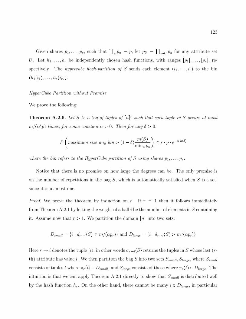
123
Given shares p1, . . . , pr, such that±
u pu p, let pU ±
uPU pu for any attribute set
U . Let h1, . . . , hr be independently chosen hash functions, with ranges rp1s, . . . , rprs, re-
spectively. The hypercube hash-partition of S sends each element pi1, . . . , irq to the bin
ph1pi1q, . . . , hrpirqq.
HyperCube Partition without Promise
We prove the following:
Theorem A.2.6. Let S be a bag of tuples of rnsr such that each tuple in S occurs at most
mpαrpq times, for some constant α ¡ 0. Then for any δ ¡ 0:
P
maximum size any bin ¡ p1 δq mpSq
minu pu
¤ r p eαhpδq
where the bin refers to the HyperCube partition of S using shares p1, . . . , pr.
Notice that there is no promise on how large the degrees can be. The only promise is
on the number of repetitions in the bag S, which is automatically satisfied when S is a set,
since it is at most one.
Proof. We prove the theorem by induction on r. If r 1 then it follows immediately
from Theorem A.2.1 by letting the weight of a ball i be the number of elements in S containing
it. Assume now that r ¡ 1. We partition the domain rns into two sets:
Dsmall ti | dr ÞÑipSq ¤ mpαprqu and Dlarge ti | dr ÞÑipSq ¡ mpαprqu
Here r ÞÑ i denotes the tuple piq; in other words σr ÞÑipSq returns the tuples in S whose last (r-
th) attribute has value i. We then partition the bag S into two sets Ssmall, Slarge, where Ssmall
consists of tuples t where πrptq P Dsmall, and Slarge consists of those where πrptq P Dlarge. The
intuition is that we can apply Theorem A.2.1 directly to show that Ssmall is distributed well
by the hash function hr. On the other hand, there cannot be many i P Dlarge, in particular
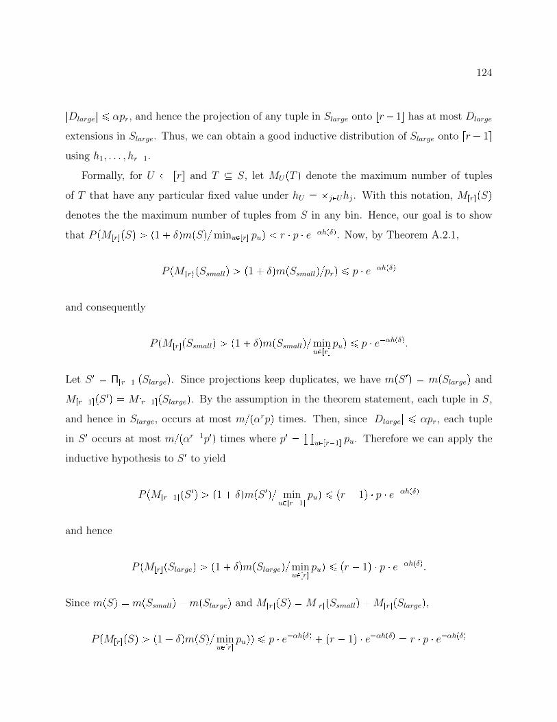
124
|Dlarge| ¤ αpr, and hence the projection of any tuple in Slarge onto rr 1s has at most Dlarge
extensions in Slarge. Thus, we can obtain a good inductive distribution of Slarge onto rr 1susing h1, . . . , hr1.
Formally, for U rrs and T S, let MUpT q denote the maximum number of tuples
of T that have any particular fixed value under hU jPUhj. With this notation, MrrspSqdenotes the the maximum number of tuples from S in any bin. Hence, our goal is to show
that P pMrrspSq ¡ p1 δqmpSqminuPrrs puq r p eαhpδq. Now, by Theorem A.2.1,
P pMtrupSsmallq ¡ p1 δqmpSsmallqprq ¤ p eαhpδq
and consequently
P pMrrspSsmallq ¡ p1 δqmpSsmallqminuPrrs
puq ¤ p eαhpδq.
Let S 1 Πrr1spSlargeq. Since projections keep duplicates, we have mpS 1q mpSlargeq and
Mrr1spS 1q Mrr1spSlargeq. By the assumption in the theorem statement, each tuple in S,
and hence in Slarge, occurs at most mpαrpq times. Then, since |Dlarge| ¤ αpr, each tuple
in S 1 occurs at most mpαr1p1q times where p1 ±uPrr1s pu. Therefore we can apply the
inductive hypothesis to S 1 to yield
P pMrr1spS 1q ¡ p1 δqmpS 1q minuPrr1s
puq ¤ pr 1q p eαhpδq
and hence
P pMrrspSlargeq ¡ p1 δqmpSlargeqminuPrrs
puq ¤ pr 1q p eαhpδq.
Since mpSq mpSsmallq mpSlargeq and MrrspSq MrrspSsmallq MrrspSlargeq,
P pMrrspSq ¡ p1 δqmpSqminuPrrs
puqq ¤ p eαhpδq pr 1q eαhpδq r p eαhpδq
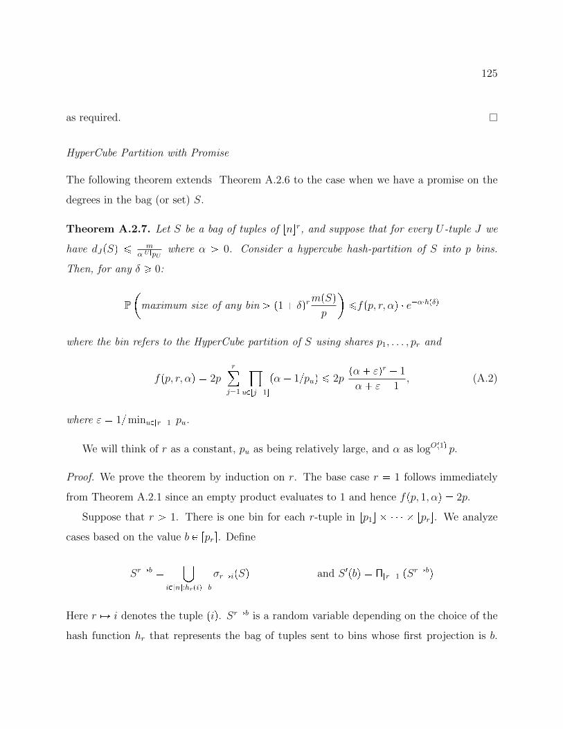
125
as required.
HyperCube Partition with Promise
The following theorem extends Theorem A.2.6 to the case when we have a promise on the
degrees in the bag (or set) S.
Theorem A.2.7. Let S be a bag of tuples of rnsr, and suppose that for every U-tuple J we
have dJpSq ¤ mα|U |pU
where α ¡ 0. Consider a hypercube hash-partition of S into p bins.
Then, for any δ ¥ 0:
P
maximum size of any bin ¡ p1 δqrmpSqp
¤fpp, r, αq eαhpδq
where the bin refers to the HyperCube partition of S using shares p1, . . . , pr and
fpp, r, αq 2pr
j1
¹uPrj1s
pα 1puq ¤ 2ppα εqr 1
α ε 1, (A.2)
where ε 1minuPrr1s pu.
We will think of r as a constant, pu as being relatively large, and α as logOp1q p.
Proof. We prove the theorem by induction on r. The base case r 1 follows immediately
from Theorem A.2.1 since an empty product evaluates to 1 and hence fpp, 1, αq 2p.
Suppose that r ¡ 1. There is one bin for each r-tuple in rp1s rprs. We analyze
cases based on the value b P rprs. Define
SrÑb ¤
iPrns:hrpiqb
σr ÞÑipSq and S 1pbq Πrr1spSrÑbq
Here r ÞÑ i denotes the tuple piq. SrÑb is a random variable depending on the choice of the
hash function hr that represents the bag of tuples sent to bins whose first projection is b.
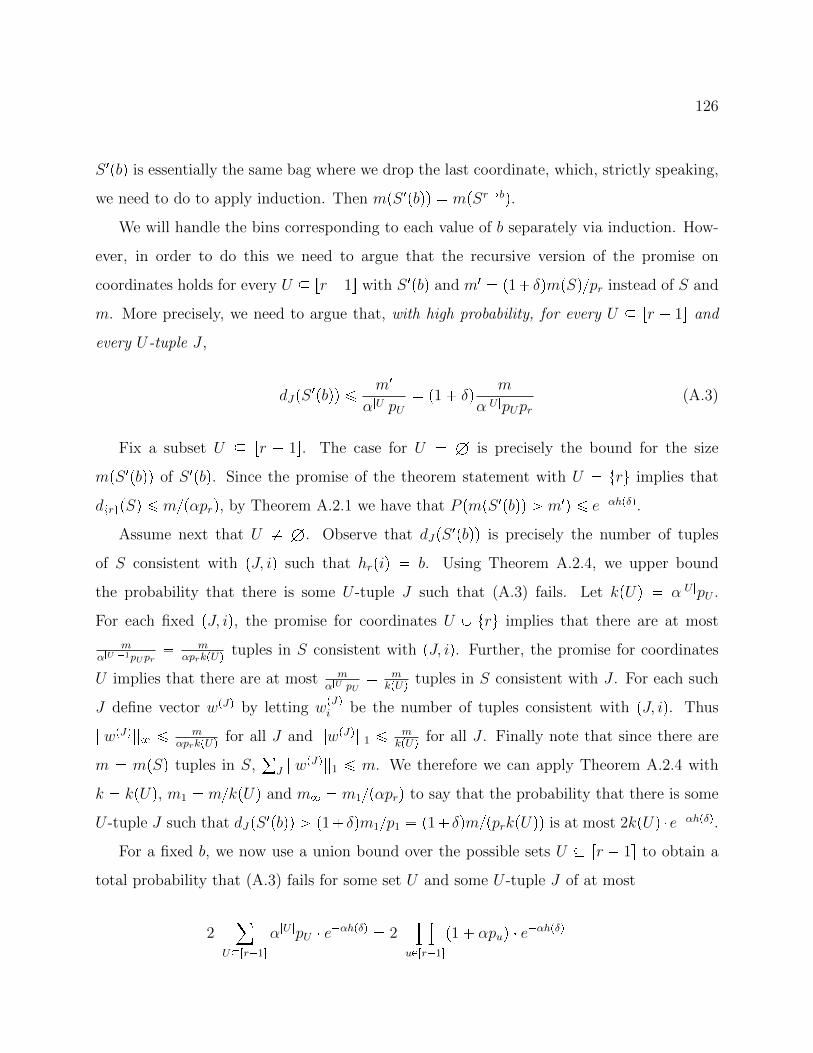
126
S 1pbq is essentially the same bag where we drop the last coordinate, which, strictly speaking,
we need to do to apply induction. Then mpS 1pbqq mpSrÑbq.We will handle the bins corresponding to each value of b separately via induction. How-
ever, in order to do this we need to argue that the recursive version of the promise on
coordinates holds for every U rr 1s with S 1pbq and m1 p1 δqmpSqpr instead of S and
m. More precisely, we need to argue that, with high probability, for every U rr 1s and
every U-tuple J ,
dJpS 1pbqq ¤ m1
α|U |pU p1 δq m
α|U |pUpr(A.3)
Fix a subset U rr 1s. The case for U H is precisely the bound for the size
mpS 1pbqq of S 1pbq. Since the promise of the theorem statement with U tru implies that
dtrupSq ¤ mpαprq, by Theorem A.2.1 we have that P pmpS 1pbqq ¡ m1q ¤ eαhpδq.
Assume next that U H. Observe that dJpS 1pbqq is precisely the number of tuples
of S consistent with pJ, iq such that hrpiq b. Using Theorem A.2.4, we upper bound
the probability that there is some U -tuple J such that (A.3) fails. Let kpUq α|U |pU .
For each fixed pJ, iq, the promise for coordinates U Y tru implies that there are at most
mα|U |1pUpr
mαprkpUq
tuples in S consistent with pJ, iq. Further, the promise for coordinates
U implies that there are at most mα|U |pU
mkpUq
tuples in S consistent with J . For each such
J define vector wpJq by letting wpJqi be the number of tuples consistent with pJ, iq. Thus
||wpJq||8 ¤ mαprkpUq
for all J and ||wpJq||1 ¤ mkpUq
for all J . Finally note that since there are
m mpSq tuples in S,°J ||wpJq||1 ¤ m. We therefore we can apply Theorem A.2.4 with
k kpUq, m1 mkpUq and m8 m1pαprq to say that the probability that there is some
U -tuple J such that dJpS 1pbqq ¡ p1 δqm1p1 p1 δqmpprkpUqq is at most 2kpUq eαhpδq.For a fixed b, we now use a union bound over the possible sets U rr 1s to obtain a
total probability that (A.3) fails for some set U and some U -tuple J of at most
2¸
Urr1s
α|U |pU eαhpδq 2¹
uPrr1s
p1 αpuq eαhpδq
127
2ppprq¹
uPrr1s
pα 1puq eαhpδq
If mpS 1pbqq ¤ m1 and (A.3) holds for all U rr 1s and U -tuples J , then we apply
the induction hypothesis (A.2) to derive that the probability that some bin that has b in
its last coordinate has more than p1 δqr1m1ppprq p1 δqrmp tuples is at most
fpppr, r 1, αq eαhpδq.Since there are pr choices for b, we obtain a total failure probability at most g eαhpδq
where
g pr
2prr1s
¹uPrr1s
pα 1puq fpppr, r 1, αq
2p¹
uPrr1s
pα 1puq pr fpppr, r 1, αq
2p¹
uPrr1s
pα 1puq prp2pprqr1
j1
¹uPrj1s
pα 1puq
2pr
j1
¹uPrj1s
pα 1puq
fpp, r, αq
The final bound uses geometric series sum upper bound.
128
VITA
Paraschos Koutris was born in Athens, Greece, on July 13, 1986. After graduating from
Ionios High School in 2004, he studied Electrical and Computer Engineering at the National
Technical University of Athens, from where he received a Diploma in 2009. He completed a
Master of Science in Logic, Algorithms and Computation at the University of Athens in 2010,
with a thesis titled ”Infrastructure Leasing Problems”. He entered the graduate program in
Computer Science and Engineering at the University of Washington, Seattle, in 2010.