Embed Size (px)
Citation preview
A NOVEL NUMERICAL ANALYSIS OF HALL EFFECT
THRUSTER AND ITS APPLICATION IN SIMULTANEOUS DESIGN
OF THRUSTER AND OPTIMAL LOW-THRUST TRAJECTORY
A Dissertation Presented to
The Academic Faculty
by
Kybeom Kwon
In Partial Fulfillment of the Requirements for the Degree
Doctor of Philosophy in the School of Aerospace Engineering
Georgia Institute of Technology August 2010
COPYRIGHT © 2010 BY KYBEOM KWON
A NOVEL NUMERICAL ANALYSIS OF HALL EFFECT
THRUSTER AND ITS APPLICATION IN SIMULTANEOUS DESIGN
OF THRUSTER AND OPTIMAL LOW-THRUST TRAJECTORY
Approved by:
Dr. Dimitri N. Mavris Advisor (Committee Chair), Professor School of Aerospace Engineering Director of Aerospace Systems Design Laboratory Georgia Institute of Technology
Dr. Justin Koo Propulsion Directorate Air Force Research Laboratory Edwards AFB
Dr. Mitchell L. R. Walker Co-Advisor, Assistant Professor School of Aerospace Engineering Director of High Power Electric Propulsion Laboratory Georgia Institute of Technology
Dr. Taewoo Nam Research Engineer II School of Aerospace Engineering Aerospace Systems Design Laboratory Georgia Institute of Technology
Dr. Ryan P. Russell Co-Advisor, Assistant Professor School of Aerospace Engineering Space Systems Design Laboratory Georgia Institute of Technology
Date Approved U July 2, 2010

iii
DEDICATION
To the space pioneers and my wife

iv
ACKNOWLEDGEMENTS
I would like to thank my committee for their advice and support. This work
couldn’t have been done without their efforts. Most of all, I truly appreciate that Dr.
Mavris, my advisor, accepted me as his student, supported me and allowed me to do this
research. It is really an honor for me to be one of your students. I am also grateful that my
co-advisors, Dr. Walker and Dr. Russell, have generously shared their priceless
accumulated knowledge with me. Thanks to Dr. Koo for your thorough review on my
proposal and thesis documents. I remember fondly the discussions with Dr. Nam and his
kind guidance.
I am also grateful to my friend, Gregory. Our friendship extended beyond that of a
collaborator of this thesis. I will always be grateful for your help and I will always feel
that I have done little for you in return. I cannot find the words to express how important
your friendship has been and I will never forget what you have done for me depite the
cultural difference. I will never forget what you have done for me.
I would like to sincerely thank the Republic of Korea Air Force for the support.
There are also many colleagues to which I would like to extend my appreciation for;
Korean colleagues, the ASDL project teams I have worked on, people in other Aerospace
Engineering labs. I thank you all.
I also want to give warm hugs to my beloved wife Insoon, who gave me full
support during hard times over the past 5 years while bringing up two sons, and my
loving parents who still think me as their child to be taken care of.
In my office desk, Atlanta, GA, Summer 2010
v
TABLE OF CONTENTS
Page
DEDICATION.................................................................................................................. iii
ACKNOWLEDGEMENTS ............................................................................................ iv
LIST OF TABLES .............................................................................................................x
LIST OF FIGURES ....................................................................................................... xiii
LIST OF SYMBOLS ..................................................................................................... xix
LIST OF ABBREVIATIONS ..................................................................................... xxvi
SUMMARY .................................................................................................................. xxix
CHAPTER 1 INTRODUCTION ....................................................................................1
1.1 Space Propulsion ....................................................................................................1
1.2 Electric Propulsion (EP) .........................................................................................5
1.3 Hall Effect Thruster ..............................................................................................10
1.4 Interim Summary ..................................................................................................14
1.5 General Remarks on a New HET Design .............................................................14
1.6 Previous Design Activities for HET .....................................................................15
1.6.1 Case Study I – University of Michigan / AFRL P5 5 kW class HET Design ............................................................................................................16
1.6.2 Case Study II – More Recently Suggested Scaling Laws and Design Process ...........................................................................................................20
1.6.3 Concluding Remarks on Case Studies ........................................................25
1.7 Low-Thrust Trajectory Optimization ...................................................................25
1.8 Motivation .............................................................................................................27
1.9 Research Objectives ..............................................................................................29
1.10 Research Questions .............................................................................................30

vi
1.11 Collaboration and Thesis Organization ..............................................................32
CHAPTER 2 THEORETICAL FOUNDATION ........................................................34
2.1 Understanding Basic Mathematical Modeling for HET .......................................34
2.2 Understanding Basic Low-Thrust Trajectory Optimization .................................46
CHAPTER 3 LITERATURE REVIEW AND PHYSICS-BASED ANALYSIS TOOL IDENTIFICATION FOR HET ..........................................................................50
3.1 Criteria for Conceptual Physics-Based Analysis Tool for HET ...........................50
3.2 Previous Work on HET Numerical Modeling ......................................................51
3.2.1 Full Kinetic Modeling ................................................................................51
3.2.2 Hybrid Modeling ........................................................................................52
3.2.3 Full Fluid Modeling ....................................................................................53
3.2.4 Other Methods ............................................................................................56
3.3 Tool Identification ................................................................................................57
CHAPTER 4 PHYSICS-BASED ANALYSIS TOOL DEVELOPMENT FOR HET ...................................................................................................................................59
4.1 Hypotheses for an Intended Tool ..........................................................................59
4.2 Ideas to Meet the Criteria .....................................................................................60
4.2.1 Assurance of Numerical Efficiency ............................................................60
4.2.2 Assurance of Numerical Robustness ..........................................................61
4.2.3 Assurance of Self-Consistency ...................................................................64
4.2.4 Assurance of Physics Representativeness ..................................................67
4.3 Development of Physics-based Analysis Tool .....................................................71
4.3.1 Analysis Domain ........................................................................................71
4.3.2 Assumptions ...............................................................................................71
4.3.3 Expected Solution Structure for Electric Potential Distribution ................73
4.3.4 Anode Sheath Region .................................................................................74
vii
4.3.5 Presheath Region ........................................................................................76
4.3.6 Ionization/Acceleration Region ..................................................................85
4.3.7 Matching Two Solutions ............................................................................95
4.3.8 Non-Dimensionalization .............................................................................98
CHAPTER 5 VALIDATION AND TOOL CAPABILITY STUDY .........................99
5.1 Point Validation with the SPT-100 .......................................................................99
5.1.1 SPT-100 Thruster .......................................................................................99
5.1.2 Comparisons of the Performance Metrics ................................................101
5.1.3 Convergence Characteristics ....................................................................103
5.1.4 Plasma Structures .....................................................................................104
5.2 Limitations of the Developed Tool .....................................................................107
5.2.1 Accuracy of the Plasma Structures ...........................................................108
5.2.2 Variation of Magnetic Field Distribution .................................................109
5.3 Validation at Other Operating Points of the SPT-100 ........................................110
5.3.1 Remarks on the Proposed Modeling of the Anomalous Coefficients ......110
5.3.2 Redefinition of Performance Metrics .......................................................111
5.3.3 Validation with Fixed Anomalous Coefficients .......................................115
5.3.4 Classification of Solutions Obtained from the Developed Tool ..............117
5.3.5 Construction of Design of Experiment (DOE) Environment ...................121
5.3.6 Numerical Exploration for the Ranges of the Anomalous Coefficients ...122
5.3.7 Validation with Optimum Anomalous Coefficients .................................129
5.4 Pseudo-Validation with the High Power Class HETs ........................................134
5.4.1 Validation with the T-220 Hall Effect Thruster .......................................134
5.4.2 Validation with the NASA-457M Hall Effect Thruster ...........................146
5.5 Sensitivity Studies for the SPT-100 ....................................................................157
viii
5.6 Approximation of the Radial Magnetic Field Distribution with the Given Performance Goals ....................................................................................................159
CHAPTER 6 DESIGN SPACE EXPLORATION FOR HET .................................164
6.1 Need of Design Space Exploration .....................................................................164
6.2 Design Space Exploration for the HET ..............................................................165
6.2.1 Selection of the Design Space ..................................................................165
6.2.2 Design Space Exploration Strategy ..........................................................167
6.2.3 Constraints on Feasible Thruster Operation .............................................168
6.2.4 Analysis of the DSE Results .....................................................................170
CHAPTER 7 CONSTRUCTION OF SURROGATE MODELS FOR HET .........179
7.1 Surrogate Models ................................................................................................179
7.2 Surrogate Models for Performance Metrics using Response Surface Methodology .............................................................................................................180
7.3 Neural Network Implementation for Performance Metric Surrogate Models ....183
7.4 Surrogate Models for Constraints .......................................................................190
7.4.1 General Considerations on Constraints ....................................................190
7.4.2 Use of Response Surface Methodology ...................................................192
7.4.3 Constraints as a Classification ..................................................................195
7.4.4 Support Vector Machine Classifier as a Constraint Function ..................197
CHAPTER 8 SIMULTANEOUS DESIGN OPTIMIZATION FOR AN ELECTRIC ORBIT RAISING MISSION BY COLLABORATION WORK .........206
8.0 Acknowledgement ..............................................................................................206
8.1 Mission Selection ................................................................................................206
8.2 Electric Orbit Raising Mission Description ........................................................208
8.3 Simultaneous Design Optimization Environment ..............................................211
8.4 Results and Comparisons ....................................................................................216
ix
8.4.1 Case of lower limit 1d for the SVM Classifier Constraint Limit .................216
8.4.2 Case of lower limit 3d for the SVM Classifier Constraint Limit ................222
8.4.3 Optimal Low-Thrust Trajectory Calculation with the SPT-100 Thruster ........................................................................................................230
8.4.4 Comparison with Pure Chemical Transfer ...............................................235
CHAPTER 9 CONCLUSIONS AND FUTURE WORK .........................................239
9.1 Conclusions .........................................................................................................239
9.2 Contributions ......................................................................................................243
9.3 Future Work ........................................................................................................245
APPENDIX A. APPROXIMATION OF AZIMUTHAL ELECTRON MEAN VELOCITY USING LANGEVIN’S APPROACH .....................................................247
APPENDIX B. CURVE-FIT EQUATIONS FOR REACTION RATES ................251
APPENDIX C. REFERENCE VALUES FOR NON-DIMENSIONALIZATION OF VARIABLES ............................................................................................................255
APPENDIX D. DESCRIPTION OF THE DEVELOPED TOOL: HOW-TO-USE ...............................................................................................................257
REFERENCES ...............................................................................................................265
VITA................................................................................................................................281
x
LIST OF TABLES
Page
Table 1.1: Available Space Propulsion Technology Options [1] - [3] ................................2
Table 1.2: Available Electric Propulsion Options and Their Characteristics [1] - [3] ........7
Table 1.3: Metrics and Parameters of Interest in HET Design ..........................................15
Table 2.1: Continuous Nonlinear Optimal Controller [58] ................................................48
Table 3.1: Tool Identification based on the Criteria ..........................................................58
Table 5.1: Geometry and Input Parameters of SPT-100 ..................................................100
Table 5.2: Comparisons of Calculated Metrics ................................................................102
Table 5.3: Experimental Performance Data of the SPT-100 [16] ....................................115
Table 5.4: Summary of Fit for Thrust ..............................................................................124
Table 5.5: Parameter Estimates and Associated Pareto Plot for Thrust ..........................125
Table 5.6: Parameter Estimates and Associated Pareto Plot for Discharge Current .......126
Table 5.7: Summary of Fit for Total Efficiency ..............................................................126
Table 5.8: Parameter Estimates and Associated Pareto Plot for Total Efficiency ...........127
Table 5.9: Comparison Results with Fixed and Optimum ,ˆ
ano in and out ............................132
Table 5.10: Operation Conditions and Geometry of the T-220 .......................................135
Table 5.11: Ranges of Magnetic Field Parameters ..........................................................137
Table 5.12: Validation Results for the T-220 Design Operating Point ............................138
Table 5.13: Performance Metric Distributions ................................................................144
Table 5.14: Performance Metric Distributions at Optimum Magnetic Field Distribution ......................................................................................................145
Table 5.15: Operation Conditions and Geometry of the NASA-457M (est: estimation) ................................................................................................147
Table 5.16: Experimental Data of the NASA-457M [128] (Thrust Error = ± 1%) .........149

xi
Table 5.17: Goodness of Fit for the NASA-457M DOEs ................................................150
Table 5.18: Validation Results for the NASA-457M ......................................................151
Table 5.19: Validation Results for the NASA-457M with All 4 Points ..........................155
Table 5.20: Effect on Multiply-Charged Ions ..................................................................157
Table 5.21: Variables and Ranges of Sensitivity Studies for the SPT-100 .....................158
Table 5.22: Operation Conditions and Geometry of the P5 .............................................160
Table 5.23: The P5 Performance Metrics at Design Operation Point ..............................161
Table 5.24: Ranges of Magnetic Field Parameters for the P5 .........................................161
Table 5.25: Results of Finding Candidate Radial Magnetic Field Distribution ..............162
Table 6.1: Ranges of Variables ........................................................................................167
Table 6.2: DOE Cases and Results ..................................................................................168
Table 6.3: Performance Metric Distributions of the Design Space .................................171
Table 7.1: Goodness of Fit Results ..................................................................................182
Table 7.2: Validation and Test Data Sets .........................................................................185
Table 7.3: Goodness of Fit for the Constraints ................................................................192
Table 7.4: Test Results of Constraint Surrogate Models .................................................192
Table 7.5: Goodness of Fit with All Cases ......................................................................193
Table 7.6: Test Results of Constraint Surrogate Models with All Cases .........................194
Table 8.1: Initial and Final Orbits of EOR ......................................................................210
Table 8.2: Constraints for Each Trajectory Segment .......................................................216
Table 8.3: SNOPT options ...............................................................................................216
Table 8.4: Design Results for lower limit 1d ......................................................................216
Table 8.5: Convergence Property for lower limit 3d ..........................................................223
Table 8.6: Design Results for lower limit 3d ......................................................................223
Table 8.7: Results of Monte Carlo Simulation ................................................................229

xii
Table 8.8: Convergence Property for the SPT-100 ..........................................................230
Table 8.9: Comparison of Design Results with SPT-100 ................................................234
Table 8.10: Comparison with Bipropellant Liquid Rocket Transfer for EOR ................236
Table 8.11: Comparison of Pure Chemical Transfer and C-EOR ...................................237
Table 8.12: GEO Delivery Cost Estimation [151] ...........................................................238
xiii
LIST OF FIGURES
Page
Figure 1.1: Final Mass Fraction Comparison (Isp of EP = 2000 sec, Isp of CP = 400 sec) ..5
Figure 1.2: Baseline Dawn Mission [4] ...............................................................................6
Figure 1.3: The Schematic of Hall Effect Thruster (SPT) .................................................11
Figure 1.4: The Sectional View of a Hall Effect Thruster (SPT) ......................................11
Figure 1.5: Relation between Thruster Power and Specific Impulse [22] .........................17
Figure 1.6: Relation between Expected Efficiency and Specific Impulse [22] .................18
Figure 1.7: Relation between Expected Discharge Chamber Diameter Squared and Propellant Mass Flow Rate [22] ........................................................................19
Figure 1.8: Lengths to be Determined [22] ........................................................................19
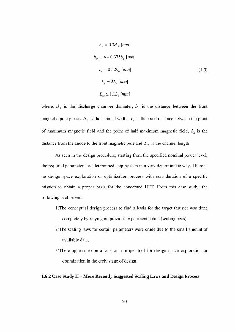
Figure 1.9: Relation between Expected Thrust and Nominal Discharge Power [24] ........21
Figure 1.10: Relation between Expected Propellant Mass Flow Rate and Nominal Discharge Power [24] ........................................................................................22
Figure 1.11: Relation between Expected Discharge Current and Propellant Mass Flow Rate [24] .............................................................................................................22
Figure 1.12: Relation between Expected Specific Impulse and Nominal Discharge Power [24] .....................................................................................................................23
Figure 1.13: Relation between Expected Efficiency and Specific Impulse [24] ...............23
Figure 1.14: Relation between Expected Channel Diameter and Nominal Discharge Power [24] ..........................................................................................................24
Figure 1.15: Relation between Expected Thruster Mass and Nominal Discharge Power [24] .....................................................................................................................24
Figure 1.16: Notional Technology S Curves on Improvement of HET Design Process ...29
Figure 1.17: Collaboration Framework..............................................................................33
Figure 2.1: Mathematical Modeling based on Kn [45] .....................................................34
Figure 2.2: Cyclotron Motion of Charged Particles [46] ...................................................36
xiv
Figure 2.3: BE
Drift of Charged Particles [46] .............................................................36
Figure 2.4: Schematic of the Sheath [54] ...........................................................................45
Figure 2.5: Plasma and Sheath Approximation [55] ..........................................................45
Figure 4.1: Solution Curves for Isothermal Euler Equations [88] .....................................61
Figure 4.2: Two Types of Anode Fall [94] ........................................................................65
Figure 4.3: Ion Current from Experimental Measurement [96] .........................................65
Figure 4.4: Electron Trajectories in Magnetic Field and Uniform Electric Field [84] ......66
Figure 4.5: Schematic of Analysis Domain .......................................................................71
Figure 4.6: Expected Solution Structure for Electric Potential ..........................................74
Figure 4.7: Schematic of Electric Potential Distribution in Anode Sheath Region ...........74
Figure 4.8: Current and Surface Charge at the Anode .......................................................75
Figure 4.9: Schematic of Sheath/Presheath Region ...........................................................76
Figure 4.10: First Ionization Cross Section for Xenon [52] ..............................................78
Figure 4.11: First Ionization Reaction Rate for Xenon ......................................................80
Figure 4.12: Non-dimensional Coordinate for Presheath Solution ....................................83
Figure 4.13: Electron-Neutral Momentum Transfer Collision Reaction Rate for Xenon .................................................................................................................88
Figure 4.14: Electron-Ion Coulomb Collision Reaction Rate ............................................89
Figure 4.15: Parameter Variation with Applied Discharge Voltage [107] ........................91
Figure 4.16: Excitation Collision Reaction Rate for Xenon ..............................................94
Figure 4.17: Diagram of Implementation of Solution Strategy .........................................97
Figure 5.1: Picture of SPT-100 (left) [120] and Computational Domain (right) [119] .....99
Figure 5.2: Magnetic Field Distribution [119] .................................................................100
Figure 5.3: Error Convergence History ...........................................................................103
Figure 5.4: Convergence History of Isp (left) and Thrust (right) .....................................104

xv
Figure 5.5: Neutral (left) and Plasma (right) Number Density Distributions ..................105
Figure 5.6: Electric Potential (left) and Electric Field (right) Distributions ....................105
Figure 5.7: Electron Temperature (left) and Ion Mean Velocity (right) Distributions ....106
Figure 5.8: Global Continuity (left) and Current Continuity (right) ................................106
Figure 5.9: Ionization Rate (left) and Electron Hall Parameter (right) Distributions ......107
Figure 5.10: Plasma Number Density (left) and Electron Velocity (right) Distributions 108
Figure 5.11: Variation of Magnetic Field Distribution with K ......................................109
Figure 5.12: UM/AFRL P5 Centerline Properties [121] .................................................110
Figure 5.13: Validation results of the SPT-100 with the anode mass flow rate variation ...........................................................................................................116
Figure 5.14. Error Behavior (left) and Specific Impulse Convergent Behavior (right) ...118
Figure 5.15. Design of Experiments Environment ..........................................................122
Figure 5.16: Visualization of Solution Success(Dot)/Fail(Cross) and Success Probability ........................................................................................................124
Figure 5.17: Actual by Predicted (left) and Residual by Predicted (right) Plots for Thrust ...............................................................................................................125
Figure 5.18: Actual by Predicted (left) and Residual by Predicted (right) Plots .............126
Figure 5.19: Prediction Profiler ( 5.25 /am mg s ) .........................................................128
Figure 5.20: Prediction Profiler for Efficiencies ( 5.25 /am mg s ) ...............................129
Figure 5.21: Prediction Profiler and Desirability Function ( 5.25 /am mg s ) ...............131
Figure 5.22: Comparisons of Experiments, Fixed and Optimum Anomalous Coefficients ......................................................................................................133
Figure 5.23: Variation of ,ˆ
ano in and Cathode Flow Fraction with Anode Mass Flow
Rate ..................................................................................................................134
Figure 5.24: T-220 Hall Effect Thruster [124] ................................................................135
Figure 5.25: Approximate Radial Magnetic Field Distribution for the T-220 ................138
Figure 5.26: Prediction Profiler and Desirability Function for the T-220 .......................139
xvi
Figure 5.27: Optimization Performance Index Contour ..................................................140
Figure 5.28: Contour of Bmax [T]......................................................................................141
Figure 5.29: Contour of Bcath [T] .....................................................................................141
Figure 5.30: Contour of K ................................................................................................142
Figure 5.31: Enlarged Contour of K – Upper Side ..........................................................142
Figure 5.32: Enlarged Contour of K – Left Side ..............................................................143
Figure 5.33: Interpretation of Outlier Box Plot [125] ......................................................144
Figure 5.34: NASA-457M Hall Effect Thruster [128] ....................................................147
Figure 5.35: Schematics of CCD and LHS ......................................................................148
Figure 5.36: Performance Validation of the NASA-457M (Thrust Error of Exp. = ± 1%) .........................................................................152
Figure 5.37: Variations of Optimum Magnetic Parameters and Anomalous Coefficients ......................................................................................................152
Figure 5.38: Performance Validation of the NASA-457M with One Magnetic Field Distribution (Thrust Error of Exp. = ± 1%) .....................................................154
Figure 5.39: Variations of Anomalous Coefficients for One Magnetic Field Distribution ......................................................................................................154
Figure 5.40: Approximate Radial Magnetic Field Distribution for the NASA-457M ....155
Figure 5.41: Sensitivity Analysis Results around the SPT-100 Design Operation Point .................................................................................................................158
Figure 5.42: Actual Radial Magnetic Field Distribution of the P5 ..................................160
Figure 5.43: Actual and Candidate Radial Magnetic Field Distribution of the P5 ..........163
Figure 6.1: Electric Propulsion Spacecraft [131] .............................................................166
Figure 6.2: Scatter Plot for the Performance Metrics ......................................................172
Figure 6.3: Scatter Plot for CCD Cases with Input Variables .........................................173
Figure 6.4: Scatter Plot of the Responses for CCD Cases ...............................................174
Figure 6.5: Effect of Anode Mass Flow ...........................................................................175
xvii
Figure 6.6: Effect of Discharge Voltage ..........................................................................176
Figure 6.7: Effect of Outer Radius ...................................................................................178
Figure 7.1: HET and Trajectory Modules in the MDO Environment [130], [5] .............179
Figure 7.2: Actual by Predicted (left) and Residual by Predicted (right) Plots ...............182
Figure 7.3: Basic Structure of an Artificial Neuron [136] ...............................................183
Figure 7.4: Basic Structure of the NNs [136] ..................................................................183
Figure 7.5: Snapshot of BRAINN Program [137] ...........................................................184
Figure 7.6: NN Regression Results For Thrust, Isp_tot, tot , Id, and Pd from Top .............188
Figure 7.7: Percent Range Errors (a) Total Specific Impulse and (b) Total Efficiency ..189
Figure 7.8: General Optimization Problem ......................................................................190
Figure 7.9: Design Space and Feasible Region ...............................................................191
Figure 7.10: Actual by Predicted Plot for g1 ....................................................................193
Figure 7.11: Actual by Predicted Plot for g1 with All Cases ...........................................194
Figure 7.12: Tree-Based Method .....................................................................................196
Figure 7.13: Optimal Separating Hyperplane [140] ........................................................197
Figure 7.14: Binary Classification (left), Support Vectors and Margin (right) [143] ......198
Figure 7.15: Mapping from 1-D to 2-D [143] ..................................................................200
Figure 7.16: Correct Rate for Polynomial Kernel Function ............................................202
Figure 7.17: Correct Rate for Gaussian Radial Basis Function Kernel ...........................203
Figure 7.18: Correct Rate for Multilayer Perceptron Kernel ...........................................203
Figure 7.19: Normalized Distance Between Hyperplane and Support Vectors ...............204
Figure 8.1: One Block DM-SL Burn (Perigee Height ≥ 200 km) [153] ..........................209
Figure 8.2: Sea Launch Payload Capability – Elliptical GTO [153] ...............................209
Figure 8.3: Structure of an optimization problem in OPTIFOR ......................................212
Figure 8.4: Flow diagram of the transition function of a segment ...................................214
xviii
Figure 8.5: Operational Variable Solutions of lower limit 1d .............................................217
Figure 8.6: Performance Histories of lower limit 1d ..........................................................218
Figure 8.7: Constraint Histories of lower limit 1d ..............................................................219
Figure 8.8: Optimum Trajectory of lower limit 1d .............................................................220
Figure 8.9: Semi-Major Axis and Eccentricity Variations of lower limit 1d ......................220
Figure 8.10: Comparisons between Surrogate Models and Actual Code ( lower limit 1d ) ....................................................................................................221
Figure 8.11: Operational Variable Solutions of lower limit 3d ..........................................224
Figure 8.12: Performance Histories of lower limit 3d ........................................................225
Figure 8.13: Constraint Histories of lower limit 3d ............................................................226
Figure 8.14: Optimum Trajectory of lower limit 3d ...........................................................226
Figure 8.15: Semi-Major Axis and Eccentricity Variations of lower limit 3d ...................227
Figure 8.16: Comparisons between Surrogate Models and Actual Code ( lower limit 3d ) ...................................................................................................228
Figure 8.17: Thrust History for the SPT-100 ...................................................................231
Figure 8.18: Optimum Trajectory for the SPT-100 .........................................................232
Figure 8.19: Semi-Major Axis and Eccentricity Variations for the SPT-100 ..................232
Figure 8.20: Comparison of In-plane Thrusting Angle Variations ..................................233
Figure 8.21: Comparisons of Semi-major Axis, Eccentricity and Spacecraft Mass Variations .........................................................................................................234
Figure 8.22: Comparison of Magnetic Field Distributions ..............................................235
Figure 8.23. Pure Chemical Transfer (left) and C-EOR Transfer (right) ........................236
Figure A.1: Uniform, Stationary Magnetic and Electric Fields .......................................248

xix
LIST OF SYMBOLS
A Thruster channel area
a Semi-major axis
B
Magnetic field vector
cathB Radial magnetic field strength at the cathode
maxB Maximum radial magnetic field strength
B Magnetic field strength difference between BRmaxR and BRcath
lower limitd Lower bound of support vector machine constraint
dt Time interval
dz Length of one computational grid cell
E
Electric field vector
e Electrical charge or eccentricity
F
Force vector
f Particle distribution function
g Constraint function
eg Magnitude of gravitational acceleration at Earth’s surface
bI Beam current
dI Discharge current
spI Specific impulse
,sp anoI Anode specific impulse
,sp totI Total specific impulse
i Orbit Inclination

xx
j
Electric current density vector
hallj
Hall current density vector
Kn Knudsen number
K Radial magnetic field shape coefficient
k Boltzmann constant
L Thruster channel length
cathL Distance from thruster exit to cathode location
sL Smooth transition distance for the anomalous coefficients
thrusterM Thruster mass
iM Ion Mach number
m Mass of particle
m Propellant mass flow rate
am Anode mass flow rate
cm Cathode mass flow rate
finalm Final space vehicle mass
initialm Initial space vehicle mass
totm Total mass flow rate
( )N t Unit normal distribution at time t
n
Unit vector
0n Plasma number density
0en Electron number density at the matching point
en Electron number density or plasma number density

xxi
,e mn Plasma number density at the matching point
,n aven Average neutral number density in the presheath region
sn Species number density
P Required Power
availableP Available Power
collP Collision probability
dP Discharge Power
totP Total Power
cathP Power used by the cathode
magP Power used by the electric magnet
sP Stress tensor
ep Electron pressure
q
Heat transfer vector
1R Thruster inner radius
2R Thruster outer radius
2R Coefficient of determination
2adjR Adjusted coefficient of determination
RR Reaction Rate
r Radial direction coordinate
cr Cyclotron radius
er Electron gyro radius
ir Ion gyro radius
xxii
( )S z Source generation function
T Thrust
anodeT Anode temperature
cpT Charged particle temperature
,e mT Electron temperature at the matching point
eVT Electron temperature in eV
pT Plasma temperature
t Time variable
t Time step
,e cu Electron mean velocity at the cathode
,e thu Mean electron thermal velocity
,eu Azimuthal electron mean velocity
su
Species mean velocity
aiu Ion acoustic velocity
,i cu Ion mean velocity at the cathode
0iu Ion mean velocity at the matching point
0nu Constant neutral mean velocity
V Total required velocity change
( )V t Velocity random variable at time t
dV Discharge voltage
xV Velocity random variable in the direction of x
yV Velocity random variable in the direction of y

xxiii
v
Velocity vector
v Cross field velocity magnitude
exitv Exit velocity of Thruster
thv Thermal velocity
W Thruster channel width
X x position random variable
Xe Abbreviation of Xenon
x
Space coordinate
Y y position random variable
z Thruster axial coordinate
cathz Axial coordinate of cathode location from thruster exit
mz Axial coordinate of matching point
Subscript , ,e i n Electron, ion, and neutral, respectively
ano Anomalous coefficient
ˆano Inverse of anomalous coefficient
relax Relaxation coefficient
Velocity space diffusion constant
Energy loss
0 Freespace permittivity
e Electron energy
exc Threshold energy of first excitation level for Xenon
ion Threshold energy of first ionization for Xenon
xxiv
Flux
Efficiency
a Acceleration efficiency
ano Anode efficiency
b Beam efficiency
e Electrical efficiency
i Ionization efficiency
tot Total efficiency
u Utilization efficiency
Electric potential
edge Electric potential at the Tonks-Langmuir edge
d Electric potential at the anode
m Electric potential at the matching point
Debye length
Reduced mass
,e Electron cross field mobility
Collision frequency or true anomaly
B Bohm collision frequency
coll Total collision frequency
d Effective frequency for the electron axial diffusion
e Electron momentum collision frequency
,e eff Effective electron momentum collision frequency

xxv
,e Electron energy loss frequency
,e m Electron momentum collision frequency
,e w Electron wall collision frequency
ei Coulomb collision frequency
en Electron neutral momentum collision frequency
exc Excitation collision frequency
i Ionization collision frequency
,i ave Averaged ionization collision frequency
mt Momentum collision frequency
recom Recombination collision frequency
Reaction cross section
Azimuthal direction coordinate
Longitude of ascending node
e Electron Hall parameter
Argument of periapsis
c Cyclotron frequency
e Electron gyro frequency
p Plasma frequency

xxvi
LIST OF ABBREVIATIONS
AFRL Air Force Research Laboratory
ASDL Aerospace Systems Design Laboratory
BN Boron Nitride
BOL Beginning Of Life
CCD Central Composite Design
CDT Closed Drift Thrusters
C-EOR Chemical-Electric Orbit Raising
CFD Computational Fluid Dynamics
CSR Charge Saturation Regime
DC Direct Current
DDP Differential Dynamic Programming
DOE Design of Experiment
DSE Design Space Exploration
DSMC Direct Simulation Monte Carlo
EDL Entry, Descent and Landing
EOR Electric Orbit Raising
EP Electric Propulsion
FET Finite Element in Time
GD-SPS General Dynamics Space Propulsion Systems
GEO Geosynchronous Earth Orbit
GTO Geosynchronous Transfer Orbit
GRC Glenn Research Center
xxvii
HDDP Hybrid Differential Dynamic Programming
HET Hall Effect Thruster
IPS Ion Propulsion System
ITAR International Traffic in Arms Regulations
LEO Low Earth Orbit
LHS Latin Hypercube Sampling
LMSSC Lockheed Martin Space Systems Company
LS Least-Squares
LTE Local Thermodynamic Equilibrium
MC Monte Carlo
MCC Monte Carlo Collision
MFE Model Fit Error
MDO Multidisciplinary Design Optimization
MLT Magnetic Layer Thruster
MPD Magnetoplasmadynamic Thruster
MRE Model Representation Error
NLP Nonlinear Programming
NMP New Millennium Program
NN Neural Network
NSSK North South Stationkeeping
ODE Ordinary Differential Equation
ORM Orbit Raising Mission
O-U Ornstein-Uhlenbeck
PIC Particle-In-Cell
PM Particle-Mesh

xxviii
PPT Pulsed Plasma Thruster
pmc Percentage of mass flow rate at the cathode
ppc Percentage of power consumed by the cathode
ppm Percentage of power consumed by electrical magnets
QP Quadratic Programming
RMSE Root Mean Square Error
RSM Response Surface Methodology
SEE Secondary Electron Emission
SEP Solar Electric Propulsion
SMO Sequential Minimal Optimization
SPT Stationary Plasma Thruster
SSDL Space Systems Design Laboratory
SVM Support Vector Machine
TAL Thruster with Anode Layer
TPBVP Two Point Boundary Value Problem
TRL Technology Readiness Level
xxix
SUMMARY
Hall Effect Thrusters (HETs) are a form of electric propulsion device which uses
external electrical energy to produce thrust. When compared to various other electric
propulsion devices, HETs are excellent candidates for future orbit transfer and
interplanetary missions due to their relatively simple configuration, moderate thrust
capability, higher thrust to power ratio, and lower thruster mass to power ratio.
Due to the short history of HETs, the current design process of a new HET is a
largely empirical and experimental science, and this has resulted in previous designs
being developed in a narrow design space based on experimental data without systematic
investigations of parameter correlations. In addition, current preliminary low-thrust
trajectory optimizations, due to inherent difficulties in solution procedure, often assume
constant or linear performances with available power in their applications of electric
thrusters. The main obstacles come from the complex physics involved in HET
technology and relatively small amounts of experimental data. Although physical theories
and numerical simulations can provide a valuable tool for design space exploration at the
inception of a new HET design and preliminary low-thrust trajectory optimization, the
complex physics makes theoretical and numerical solutions difficult to obtain.
Numerical implementations have been quite extensively conducted in the last two
decades. An investigation of current methodologies reveals that to date, none provide a
proper methodology for a new HET design at the conceptual design stage and the coupled
low-thrust trajectory optimization.

xxx
Thus, in the first half of this work, an efficient, robust, and self-consistent
numerical method for the analysis of HETs is developed with a new approach. The key
idea is to divide the analysis region into two regions in terms of electron dynamics based
on physical intuition. Intensive validations are conducted for existing HETs from 1 kW to
50 kW classes.
The second half of this work aims to construct a simultaneous design optimization
environment though collaboration with experts in low-thrust trajectory optimization
where a new HET and associated optimal low-thrust trajectory can be designed
simultaneously. A demonstration for an orbit raising mission shows that the constructed
simultaneous design optimization environment can be used effectively and synergistically
for space missions involving HETs.
It is expected that the present work will aid and ease the current expensive
experimental HET design process and reduce preliminary space mission design cycles
involving HETs.
1
CHAPTER 1
INTRODUCTION
1.1 Space Propulsion
Space propulsion basically has two objectives; one is obviously transportation, the
other is for in-orbit usage. The space transportation objective is the same as other means
of transportation; deliver payload from some initial point to a destination, which can be
intermediate or final. For example, if a communication satellite were to be placed in
Geosynchronous Earth Orbit (GEO), a launch vehicle might be used to deliver it from the
Earth’s surface to an intermediate destination in Low Earth Orbit (LEO). Another space
propulsion device such as the upper stage rocket might then deliver it from LEO to a final
destination of GEO. For planetary landing missions, another form of space propulsion is
required for capturing the planet’s orbit and Entry, Descent and Landing (EDL). In-orbit
usage stems from the requirements for specific mission needs such as attitude
requirements of the spacecraft or solar panel array (spacecraft attitude control) and space
orbital perturbation compensation (orbital maintenance). A typical metric for the
energetic requirements of these tasks is often expressed as the amount of total required
velocity change or V .
There are several space propulsion options available to accomplish various space
mission V requirements. Some of these options are commercially available while
others are considered feasible based on laboratory research or in the state of future
2
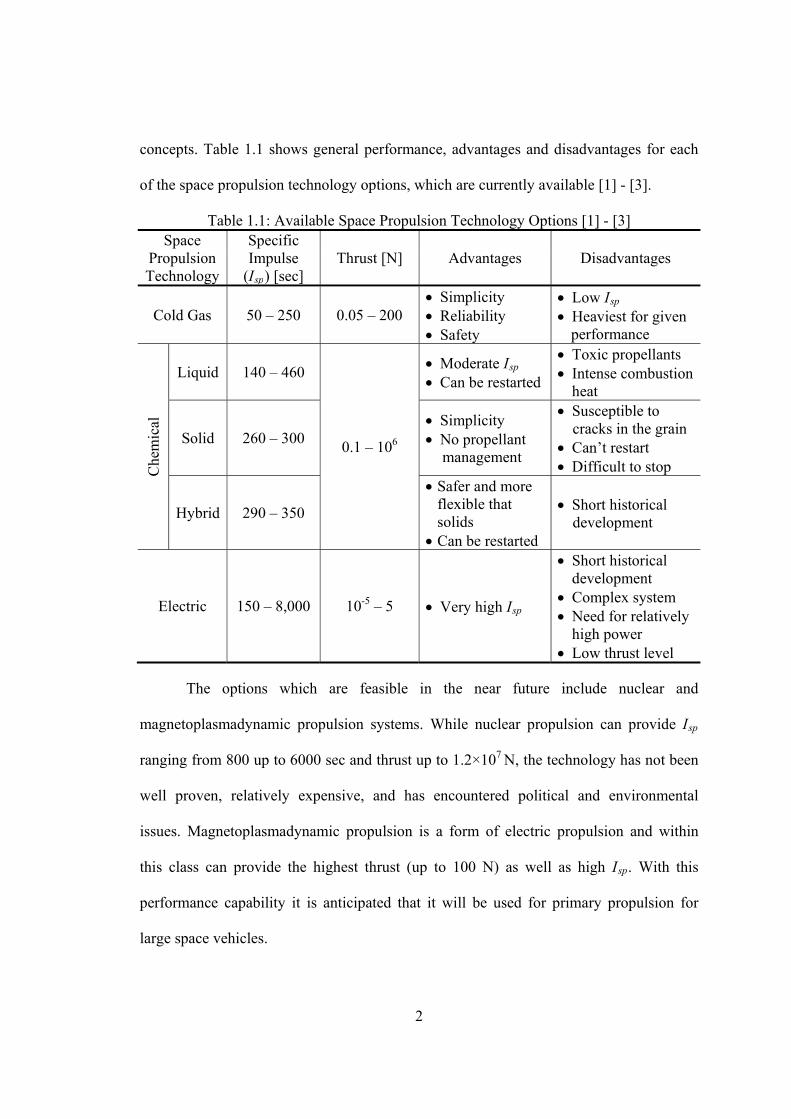
concepts. Table 1.1 shows general performance, advantages and disadvantages for each
of the space propulsion technology options, which are currently available [1] - [3].
Table 1.1: Available Space Propulsion Technology Options [1] - [3] Space
Propulsion Technology
Specific Impulse
(IRspR) [sec] Thrust [N] Advantages Disadvantages
Cold Gas 50 – 250 0.05 – 200 Simplicity Reliability Safety
Low IRsp Heaviest for given
performance
Che
mic
al
Liquid 140 – 460
0.1 – 10P
6
Moderate IRsp Can be restarted
Toxic propellants Intense combustion
heat
Solid 260 – 300 Simplicity No propellant
management
Susceptible to cracks in the grain
Can’t restart Difficult to stop
Hybrid 290 – 350
Safer and more flexible that solids
Can be restarted
Short historical development
Electric 150 – 8,000 10P
-5P – 5 Very high IRsp
Short historical development
Complex system Need for relatively
high power Low thrust level
The options which are feasible in the near future include nuclear and
magnetoplasmadynamic propulsion systems. While nuclear propulsion can provide IRspR
ranging from 800 up to 6000 sec and thrust up to 1.2×10 P
7 PN, the technology has not been
well proven, relatively expensive, and has encountered political and environmental
issues. Magnetoplasmadynamic propulsion is a form of electric propulsion and within
this class can provide the highest thrust (up to 100 N) as well as high IRspR. With this
performance capability it is anticipated that it will be used for primary propulsion for
large space vehicles.
3
Other concepts are massless propulsion devices which do not require propellants
to obtain thrust. Examples are solar sails, tethers, gravity assists, and aerobrakes.
Each propulsion system in Table 1.1 has a specific operation mechanism. Cold
gas propulsion simply uses the mechanical energy of a compressed gas propellant by
expansion through a nozzle. Chemical propulsion relies on the bond energy of propellants
through combustion. Electric propulsion uses electrical energy to accelerate the
propellant.
Referring to Table 1.1, the propulsion systems which operate in the low thrust
regime are often used for orbit maintenance, minor in-orbit maneuvers, and attitude
control. On the other hand, high thrust propulsion systems are primarily used for launch,
orbit insertion, and orbit transfers.
Specific impulse measures the efficiency of propellant usage since it is defined as
thrust divided by the propellant weight flow rate (relative to the Earth’s surface) as shown
in Equation (1.1). A high specific impulse is desirable since it gives more thrust with
given propellant mass flow rate.
spe
TI
mg
(1.1)
where, T is the thrust magnitude, m is the propellant mass flow rate, and eg is the
magnitude of the gravitational acceleration at the Earth’s surface. In the mission
perspective, specific impulse plays an important role in determining allowable payload
fractions as seen in the ideal rocket equation [2],
exp expfinal
initial exit sp e
m V V
m v I g
(1.2)

4
where, finalm is the final space vehicle mass, initialm is the initial space vehicle mass, exitv
is the exit or exhaust velocity of the thruster, and V is the required velocity change to
complete the given mission. Equation (1.2) implies that if specific impulse is high, then
for a given required velocity change, a high final mass fraction can be obtained. This is a
significant benefit since less propellant is required for the given mission.
In terms of high IRspR, electric propulsion seems to lie at the leading edge for space
propulsion. However, this is not the whole story. Due to their high thrust capability,
chemical propulsion systems are the only current viable option for launch. In addition,
orbit transfer missions have historically been performed almost exclusively by chemical
propulsion systems. However, chemical propulsion systems for other operations, such as
orbit maintenance, orbit maneuver and attitude control, are no longer the exclusive
propulsion option. Such operations do not require a large thrust capability. Rather, they
need to have the propulsion system controlled easily for precise maneuvers. Cold gas is a
good candidate for these tasks, but it has low specific impulse which implies low payload
mass fraction or short mission duration.
Electric propulsion is a leading candidate for orbit control due to its high specific
impulse capability. Furthermore, a recent study shows that if these advanced propulsion
technologies with their high specific impulse were used for general orbit transfer
missions, e.g., from LEO to GEO, significant cost savings could be realized when
compared to a conventional launch vehicle and a chemical upper stage configuration [4].
As a result, electric propulsion might be very promising for virtually all future space
propulsion except for launch. In the next section, an overview of electric propulsion will
be given.
5
1.2 Electric Propulsion (EP)
Since EP uses electrical energy to obtain thrust, the exhaust velocity produced is
not restricted by the bond energy in the propellant. Thus, exhaust velocity is not limited
in a theoretical sense, except by the speed of light. This results in a unique characteristic
of very high specific impulse. What matters is how much power can be provided to
accelerate the propellant. Therefore, a tradeoff between thrust or specific impulse and
available power is always considered.
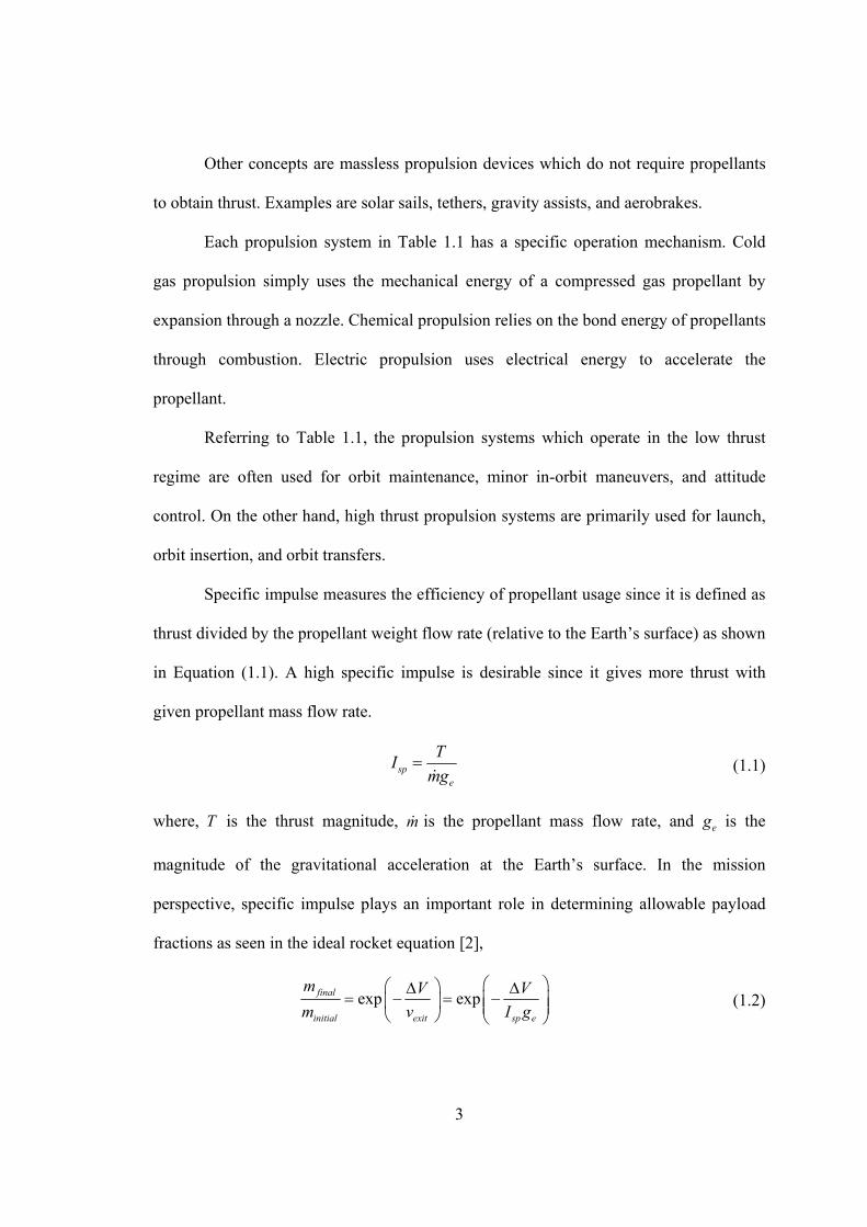
Figure 1.1: Final Mass Fraction Comparison (IRspR of EP = 2000 sec, IRspR of CP = 400 sec)
High specific impulse can expand current space mission capabilities and even
create new possibilities for future missions. This fact is more clearly shown in Figure 1.1,
which compares the final mass fractions between spacecraft using EP and chemical
propulsion using Equation (1.2). The specific impulse of EP is assumed to be 2000 sec
and that of chemical propulsion to be 400 sec.
6
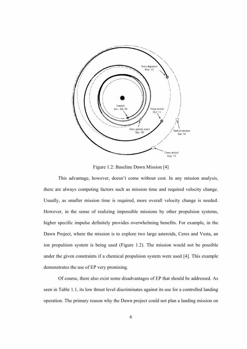
Figure 1.2: Baseline Dawn Mission [4]
This advantage, however, doesn’t come without cost. In any mission analysis,
there are always competing factors such as mission time and required velocity change.
Usually, as smaller mission time is required, more overall velocity change is needed.
However, in the sense of realizing impossible missions by other propulsion systems,
higher specific impulse definitely provides overwhelming benefits. For example, in the
Dawn Project, where the mission is to explore two large asteroids, Ceres and Vesta, an
ion propulsion system is being used (Figure 1.2). The mission would not be possible
under the given constraints if a chemical propulsion system were used [4]. This example
demonstrates the use of EP very promising.
Of course, there also exist some disadvantages of EP that should be addressed. As
seen in Table 1.1, its low thrust level discriminates against its use for a controlled landing
operation. The primary reason why the Dawn project could not plan a landing mission on
7
either Ceres or Vesta was the inability of the propulsion system to provide the 200 N
required to land on Ceres [4]. This thrust level is far beyond the capability of the current
EP devices. Furthermore, its low thrust characteristics may cause significant gravity
losses due to gradual and spiral acceleration; however this fact alone does not completely
negate its relative advantage over the chemical propulsion in terms of payload mass
fraction. Another drawback comes from its propellant acceleration mechanism. Because
electric propulsion requires an external electrical energy, additional mass for power
generation, processing and management is required, which results in a payload penalty.
Another drawback is its short development history. In spite of EP’s obvious advantages,
spacecraft designers usually prefer to use proven and highly reliable technologies rather
than those with significant uncertainties.
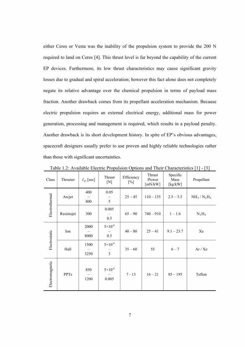
Table 1.2: Available Electric Propulsion Options and Their Characteristics [1] - [3]
Class Thruster IRspR [sec] Thrust
[N] Efficiency
[%]
Thrust /Power
[mN/kW]
Specific Mass
[kg/kW] Propellant
Ele
ctro
ther
mal
Arcjet 400
– 800
0.05 – 5
25 – 45 110 – 135 2.5 – 3.5 NHR3R / NR2RHR4
Resistojet 300 0.005
– 0.5
65 – 90 740 – 910 1 – 1.6 NR2RHR4
Ele
ctro
stat
ic
Ion 2000
– 8000
5×10P
-6
– 0.5
40 – 80 25 – 41 9.1 – 23.7 Xe
Hall 1500
– 3250
5×10P
-6P
– 3
35 – 60 55 6 – 7 Ar / Xe
Ele
ctro
mag
neti
c
PPTs 850
– 1200
5×10P
-6P
– 0.005
7 - 13 16 – 21 85 – 195 Teflon
8
Interest in EP for space propulsion started in the early 1960’s, although the
possibility had been suggested earlier [6]. Since then, a wide variety of EP devices have
been studied and developed. EP devices are classified into three categories based on their
main mechanism of accelerating propellant; electrothermal, electrostatic, and
electromagnetic. Table 1.2 shows EP classes, currently available representative thrusters,
and their characteristics.
UElectrothermal Propulsion
This category of EP has the most similar mechanism to conventional chemical
propulsion. The primary difference is that the energy required to heat the working fluid
comes from an electrical source. Conversion from heat to kinetic energy is accomplished
by a conventional nozzle as in chemical propulsion. Whereas in chemical propulsion,
heat is generated from the chemical reaction of the propellant and oxidizer, in
electrothermal propulsion, the heat is directly deposited into the working fluid by either
direct contact with resistively-heated elements (resistojet) or by passing the electric
current directly through the fluid (arcjet). Because of the limited power available, their
geometric characteristics result in small size and short nozzle length, which in turn make
the residence time of the working fluid in the nozzle small. This causes frozen flow loss
as the internal energy cannot be fully released into kinetic energy.
UElectrostatic propulsion
As implied in the name, this category of propulsion uses electrostatic fields to
accelerate the working fluid. This mechanism of obtaining thrust is quite different from
those in other space propulsion options. Since electrostatic acceleration requires at least a
partially ionized gas, the device must somehow provide the means of ionization. In
9
HETs, electron bombardment ionization is usually employed, i.e., ionization through
collisions between neutral particles and electrons. The ionization results in a plasma
consisting of atoms, electrons, and positively charged ions. Once charged particles are
generated, the ions are extracted and accelerated by an applied electrostatic field. Then a
cathode neutralizer emitting additional electrons neutralizes the accelerated ions to
prevent the spacecraft from leaving the charge equilibrium.
The ion engine has distinct regions and elements for these three processes;
ionization, ion acceleration, and ion neutralization. The ionization is done by a discharge
chamber, ion acceleration is accomplished by a series of electrically biased grids, and ion
neutralization is achieved by an additional cathode neutralizer located outside the
thruster. In contrast with the ion engine, an HET does not have distinct regions, but rather
continuous processes. Furthermore, ionization, acceleration, and neutralization are done
by a relatively simple geometric configuration when compared to ion engines. The HET
employs a magnetic field to trap electrons long enough for sufficient ionization.
Traditionally, the magnetic field has been the ubiquitous means for plasma confinement
in nuclear fusion plasma research. This is why HETs are sometimes classified as
electromagnetic propulsion. However, because the main acceleration mechanism is
electrostatic force, it seems more appropriate to classify HETs as electrostatic. Although
the efficiency of an ion thruster is the highest in terms of power conversion to useful
thrust, it suffers from a thrust density limitation (space charge constraint). In addition,
typical ion engines have a lower thrust to power ratio and higher specific mass than
HETs. In this sense, HETs are the most promising electrostatic EP device for near term
in-space propulsion. HETs will be discussed in the next section in more detail.
10
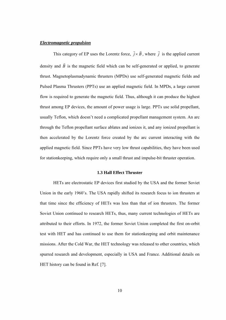
UElectromagnetic propulsion
This category of EP uses the Lorentz force, Bj
, where j
is the applied current
density and B
is the magnetic field which can be self-generated or applied, to generate
thrust. Magnetoplasmadynamic thrusters (MPDs) use self-generated magnetic fields and
Pulsed Plasma Thrusters (PPTs) use an applied magnetic field. In MPDs, a large current
flow is required to generate the magnetic field. Thus, although it can produce the highest
thrust among EP devices, the amount of power usage is large. PPTs use solid propellant,
usually Teflon, which doesn’t need a complicated propellant management system. An arc
through the Teflon propellant surface ablates and ionizes it, and any ionized propellant is
then accelerated by the Lorentz force created by the arc current interacting with the
applied magnetic field. Since PPTs have very low thrust capabilities, they have been used
for stationkeeping, which require only a small thrust and impulse-bit thruster operation.
1.3 Hall Effect Thruster
HETs are electrostatic EP devices first studied by the USA and the former Soviet
Union in the early 1960’s. The USA rapidly shifted its research focus to ion thrusters at
that time since the efficiency of HETs was less than that of ion thrusters. The former
Soviet Union continued to research HETs, thus, many current technologies of HETs are
attributed to their efforts. In 1972, the former Soviet Union completed the first on-orbit
test with HET and has continued to use them for stationkeeping and orbit maintenance
missions. After the Cold War, the HET technology was released to other countries, which
spurred research and development, especially in USA and France. Additional details on
HET history can be found in Ref. [7].
11
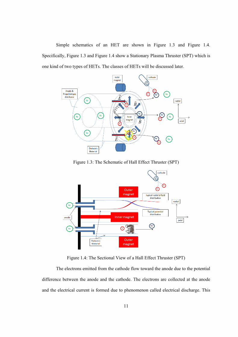
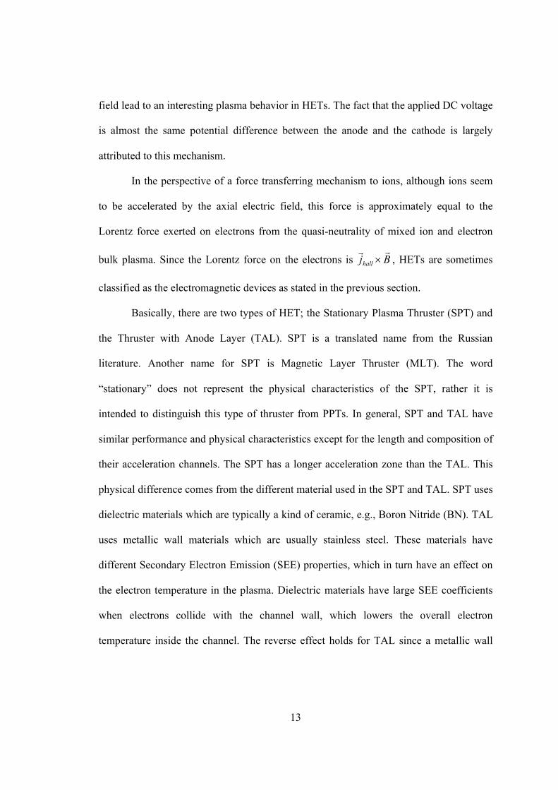
Simple schematics of an HET are shown in Figure 1.3 and Figure 1.4.
Specifically, Figure 1.3 and Figure 1.4 show a Stationary Plasma Thruster (SPT) which is
one kind of two types of HETs. The classes of HETs will be discussed later.
Figure 1.3: The Schematic of Hall Effect Thruster (SPT)
Figure 1.4: The Sectional View of a Hall Effect Thruster (SPT)
The electrons emitted from the cathode flow toward the anode due to the potential
difference between the anode and the cathode. The electrons are collected at the anode
and the electrical current is formed due to phenomenon called electrical discharge. This

12
discharge is shaped by the presence of a radial magnetic field which prohibits the
electrons from moving directly toward the anode. This is because the magnetic field has
the property of trapping the charged particles around its field lines.
Because of the axial electric field from the potential distribution between the
anode and the cathode, the Lorentz force causes the electrons to drift in the direction of
BE
, which generates an azimuthal current. This phenomenon is called the Hall effect
and the azimuthal current is called the Hall current in honor of Edwin Hall’s discovery of
this phenomenon [8]. The azimuthal current also inspired another name for HETs, Closed
Drift Thrusters (CDTs). In order to have a discharge in the device, some form of electron
transport mechanism must be present to allow the electrons to travel from the cathode to
the anode. Collisions with neutrals and other anomalous transport mechanisms provide
the mechanisms for this transport.
If a magnetic field does not exist, electrons are purely accelerated in the opposite
direction of electric field. Because the electron mass is very small, the acceleration by the
electric field causes electrons to obtain very high velocities in a very short time period.
Thus, it is expected that electrons would be transported to the anode with very high
velocity in a very short time scale, which makes it difficult to give the electrons enough
time to ionize neutrals. Through electron trapping by the magnetic field, electrons have
enough time to ionize the neutrals, i.e., raising the Damköhler number, which is the ratio
of flow times to chemical time in combustion literature. The ionization process generates
ions, which are then accelerated by the axial electric field and produce useful thrust. Ions
are nearly unaffected by the magnetic field in the distance scale of the device because of
their relatively large mass. The different responses of ions and electrons to the magnetic
13
field lead to an interesting plasma behavior in HETs. The fact that the applied DC voltage
is almost the same potential difference between the anode and the cathode is largely
attributed to this mechanism.
In the perspective of a force transferring mechanism to ions, although ions seem
to be accelerated by the axial electric field, this force is approximately equal to the
Lorentz force exerted on electrons from the quasi-neutrality of mixed ion and electron
bulk plasma. Since the Lorentz force on the electrons is Bjhall
, HETs are sometimes
classified as the electromagnetic devices as stated in the previous section.
Basically, there are two types of HET; the Stationary Plasma Thruster (SPT) and
the Thruster with Anode Layer (TAL). SPT is a translated name from the Russian
literature. Another name for SPT is Magnetic Layer Thruster (MLT). The word
“stationary” does not represent the physical characteristics of the SPT, rather it is
intended to distinguish this type of thruster from PPTs. In general, SPT and TAL have
similar performance and physical characteristics except for the length and composition of
their acceleration channels. The SPT has a longer acceleration zone than the TAL. This
physical difference comes from the different material used in the SPT and TAL. SPT uses
dielectric materials which are typically a kind of ceramic, e.g., Boron Nitride (BN). TAL
uses metallic wall materials which are usually stainless steel. These materials have
different Secondary Electron Emission (SEE) properties, which in turn have an effect on
the electron temperature in the plasma. Dielectric materials have large SEE coefficients
when electrons collide with the channel wall, which lowers the overall electron
temperature inside the channel. The reverse effect holds for TAL since a metallic wall

14
emits very few secondary electrons. This causes TALs to have very short acceleration
regions.
The extensive discussions on HET technologies are provided in Ref. [9] - [10].
The fundamental differences between SPT and TAL are discussed in depth in Ref. [11].
1.4 Interim Summary
A Top-down approach has been used to introduce background for the general
space propulsion options to the HETs. Since the current study specifically concerns HETs
in the context of its conceptual design process regarding HET performances and its
impacts on space mission trajectory optimization, the design activities for HETs and
associated low-thrust trajectory optimizations requires review. The following sections
will be devoted to these topics.
1.5 General Remarks on a New HET Design
The general design process used for aircraft or other products will apply to HETs;
conceptual, preliminary and detailed. However, in the context of the design process, how
to initiate the design process for a new HET is not an easy question due to its short
history and lack of proper design tools. The current design process of a new HET is
accomplished by empirical and experimental science. This means that specifications of
required design variables, parameters and important metrics must rely thoroughly on
previous experimental data and experience. If only historical and empirical data were to
be used, the design space to be sought would be very narrow. What makes matters worse
is that the reliance on empirical designs presents a risk for a new design which might not
be explained by previous empirical results. This risk generally comes from design trials
for either a configuration or highly nonlinear physical processes involved. The
15
configuration being designed may have major differences from what can be described by
empirical data. Highly nonlinear physical processes may also cause an unexpected and
undesirable design even though the configuration may be very similar to an existing
design. As invoked recently in the design community [12] - [13], the design processes for
a new HET must have the properties adapted into this design paradigm shift because of
the limited historical experiences, particular difficulties arising from ground test of space
propulsion devices, and highly nonlinear physical processes involved in HETs. An
important property is to bring a physics-based analysis to early design stage.
Although there are some HETs which have a Technology Readiness Level (TRL)
of 9, if one were to construct a new HET, its TRL drops significantly because of reasons
stated in the previous paragraph. General information about TRL can be found in Ref.
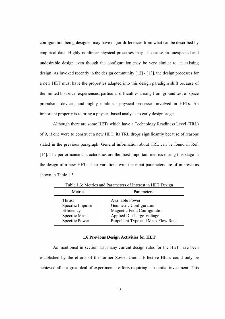
[14]. The performance characteristics are the most important metrics during this stage in
the design of a new HET. Their variations with the input parameters are of interests as
shown in Table 1.3.
Table 1.3: Metrics and Parameters of Interest in HET Design
Metrics Parameters
Thrust Specific Impulse Efficiency Specific Mass Specific Power
Available Power Geometric Configuration Magnetic Field Configuration Applied Discharge Voltage Propellant Type and Mass Flow Rate
1.6 Previous Design Activities for HET
As mentioned in section 1.3, many current design rules for the HET have been
established by the efforts of the former Soviet Union. Effective HETs could only be
achieved after a great deal of experimental efforts requiring substantial investment. This
16
seems quite ineffective compared to the current aircraft design processes. However, this
trial and error approach has been the typical process for newly proposed concepts which
are in an initial development stage.
Typical design efforts for a new HET are as follows:
1)Narrow the design space based on so called scaling laws established in the
form of graphs or empirical equations. A large number of parameters are
already determined at this step.
2)Experimental trial and error is then applied to obtain an effective HET.
Scaling laws have been proposed to aid the conceptual design process and reduce
experimental efforts. They are basically extracted from the experimental data of existing
HETs [15]-[19]. Experimental results on existing HETs can be applied to determine the
variation trend of concerned metrics for specific parameters. For example, the discharge
voltage or propellant mass flow rate can be varied for a given configuration and their
effects on metrics can be investigated. The costly parts of the design process are the
investigations necessary to determine the effects of geometric changes due to the need of
manufacturing parts of different sizes. Thus, the scaling laws for some important
geometric dimensions such as the diameter of the discharge chamber also results from
those existing HETs. Some of the detailed geometrical dimensions can be obtained
directly from the Russian Hall Thruster designers [20].
The following two sub-sections are devoted to case studies of design processes
which have been completed or proposed. The intent in presenting these case studies is to
aid in understanding the state of the art in design process of the HET.
1.6.1 Case Study I – University of Michigan / AFRL P5 5 kW class HET Design
17
University of Michigan and Air Force Research Laboratory (AFRL) designed and
built a 5kW class laboratory model HET, the UM-AFRL P5 [21]. The design process of
the P5 is summarized here [22]. Designers began by narrowing down the design using
simple equations and data from 8 existing HETs. With the targeted starting point of 5 kW
nominal power level for the target thruster, the following conceptual design process was
used.
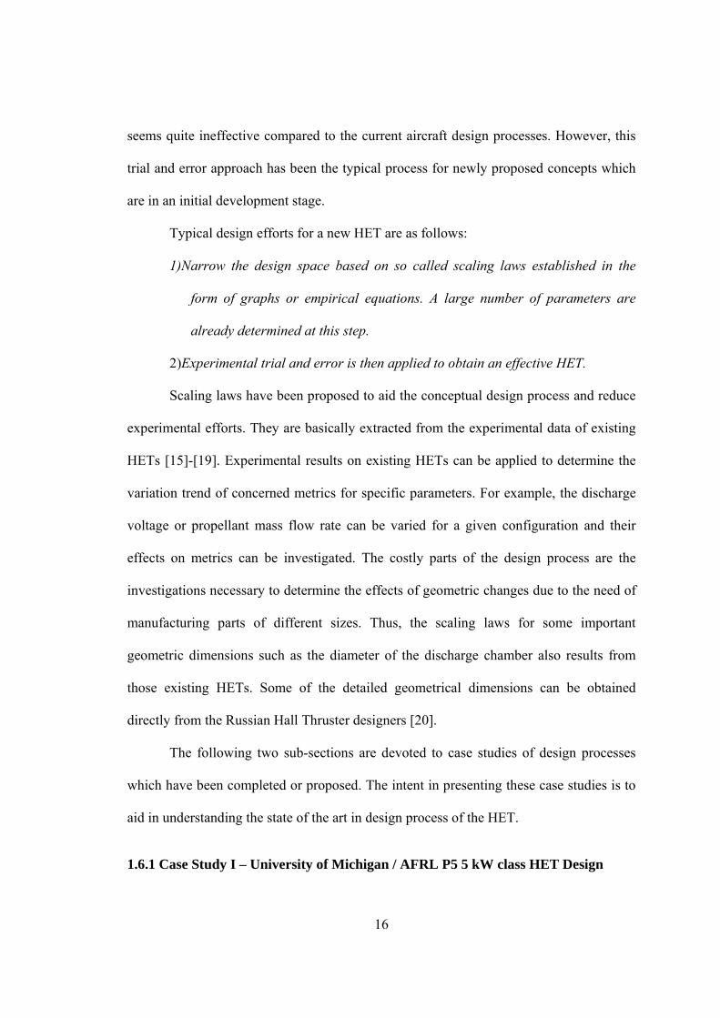
Step 1: Determine Expected Specific Impulse
An exponential scaling law from existing thrusters was used to determine the
expected specific impulse as shown in Figure 1.5.
Figure 1.5: Relation between Thruster Power and Specific Impulse [22]
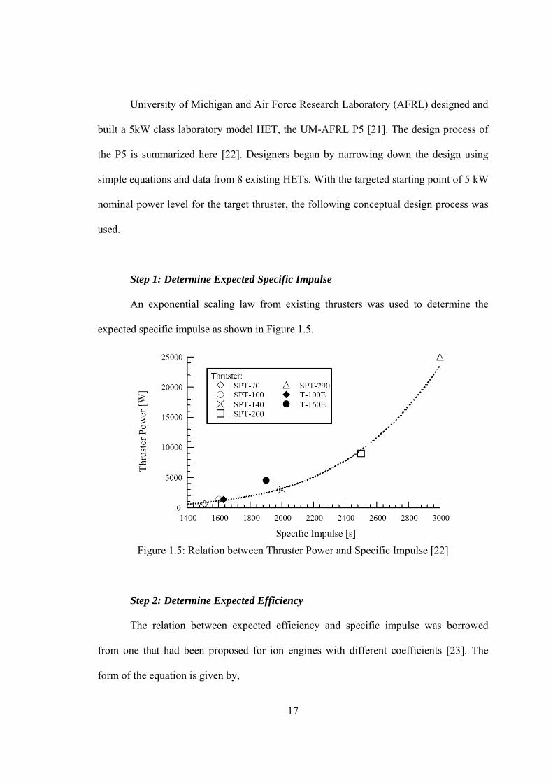
Step 2: Determine Expected Efficiency
The relation between expected efficiency and specific impulse was borrowed
from one that had been proposed for ion engines with different coefficients [23]. The
form of the equation is given by,
18
21( )e sp
ab
g I
(1.3)
where, a and b were estimated to be 0.8 and 1.42×10P
8P.
The resultant curve-fit is shown in Figure 1.6.
Figure 1.6: Relation between Expected Efficiency and Specific Impulse [22]
Step 3: Determine Expected Propellant Mass Flow Rate
The following relationship was used for the given nominal power level with
determined efficiency and specific impulse in the previous steps.
2
2
( )d
psp e
Pm
I g
(1.4)
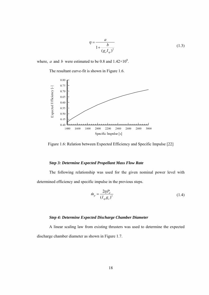
Step 4: Determine Expected Discharge Chamber Diameter
A linear scaling law from existing thrusters was used to determine the expected
discharge chamber diameter as shown in Figure 1.7.
19
Figure 1.7: Relation between Expected Discharge Chamber Diameter Squared and Propellant Mass Flow Rate [22]
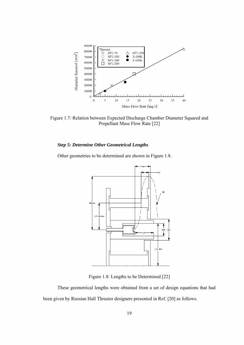
Step 5: Determine Other Geometrical Lengths
Other geometries to be determined are shown in Figure 1.8.
Figure 1.8: Lengths to be Determined [22]
These geometrical lengths were obtained from a set of design equations that had
been given by Russian Hall Thruster designers presented in Ref. [20] as follows.
20
][3.0 mmdb chm
][375.06 mmbb mch
][32.0 mmbL me
][2 mmLL ea
][1.1 mmLL ach
(1.5)
where, chd is the discharge chamber diameter, mb is the distance between the front
magnetic pole pieces, chb is the channel width, eL is the axial distance between the point
of maximum magnetic field and the point of half maximum magnetic field, aL is the
distance from the anode to the front magnetic pole and chL is the channel length.
As seen in the design procedure, starting from the specified nominal power level,
the required parameters are determined step by step in a very deterministic way. There is
no design space exploration or optimization process with consideration of a specific
mission to obtain a proper basis for the concerned HET. From this case study, the
following is observed:
1)The conceptual design process to find a basis for the target thruster was done
completely by relying on previous experimental data (scaling laws).
2)The scaling laws for certain parameters were crude due to the small amount of
available data.
3)There appears to be a lack of a proper tool for design space exploration or
optimization in the early stage of design.
1.6.2 Case Study II – More Recently Suggested Scaling Laws and Design Process
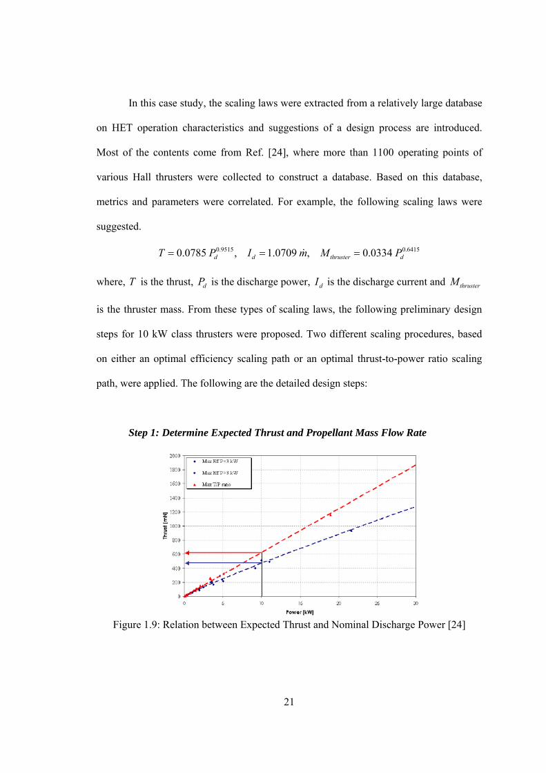
21
In this case study, the scaling laws were extracted from a relatively large database
on HET operation characteristics and suggestions of a design process are introduced.
Most of the contents come from Ref. [24], where more than 1100 operating points of
various Hall thrusters were collected to construct a database. Based on this database,
metrics and parameters were correlated. For example, the following scaling laws were
suggested.
6415.09515.0 0334.0,0709.1,0785.0 dthrusterdd PMmIPT
where, T is the thrust, dP is the discharge power, dI is the discharge current and thrusterM
is the thruster mass. From these types of scaling laws, the following preliminary design
steps for 10 kW class thrusters were proposed. Two different scaling procedures, based
on either an optimal efficiency scaling path or an optimal thrust-to-power ratio scaling
path, were applied. The following are the detailed design steps:
Step 1: Determine Expected Thrust and Propellant Mass Flow Rate
Figure 1.9: Relation between Expected Thrust and Nominal Discharge Power [24]
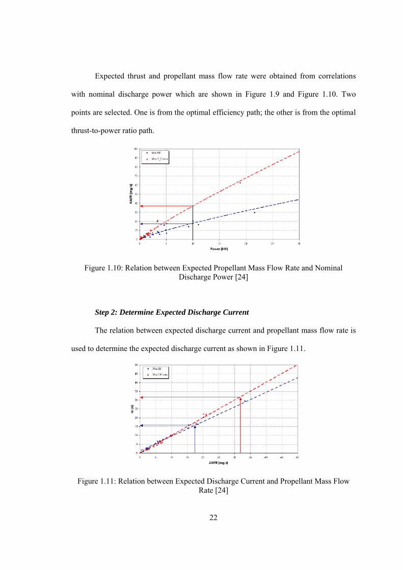
22
Expected thrust and propellant mass flow rate were obtained from correlations
with nominal discharge power which are shown in Figure 1.9 and Figure 1.10. Two
points are selected. One is from the optimal efficiency path; the other is from the optimal
thrust-to-power ratio path.
Figure 1.10: Relation between Expected Propellant Mass Flow Rate and Nominal Discharge Power [24]
Step 2: Determine Expected Discharge Current
The relation between expected discharge current and propellant mass flow rate is
used to determine the expected discharge current as shown in Figure 1.11.
Figure 1.11: Relation between Expected Discharge Current and Propellant Mass Flow Rate [24]
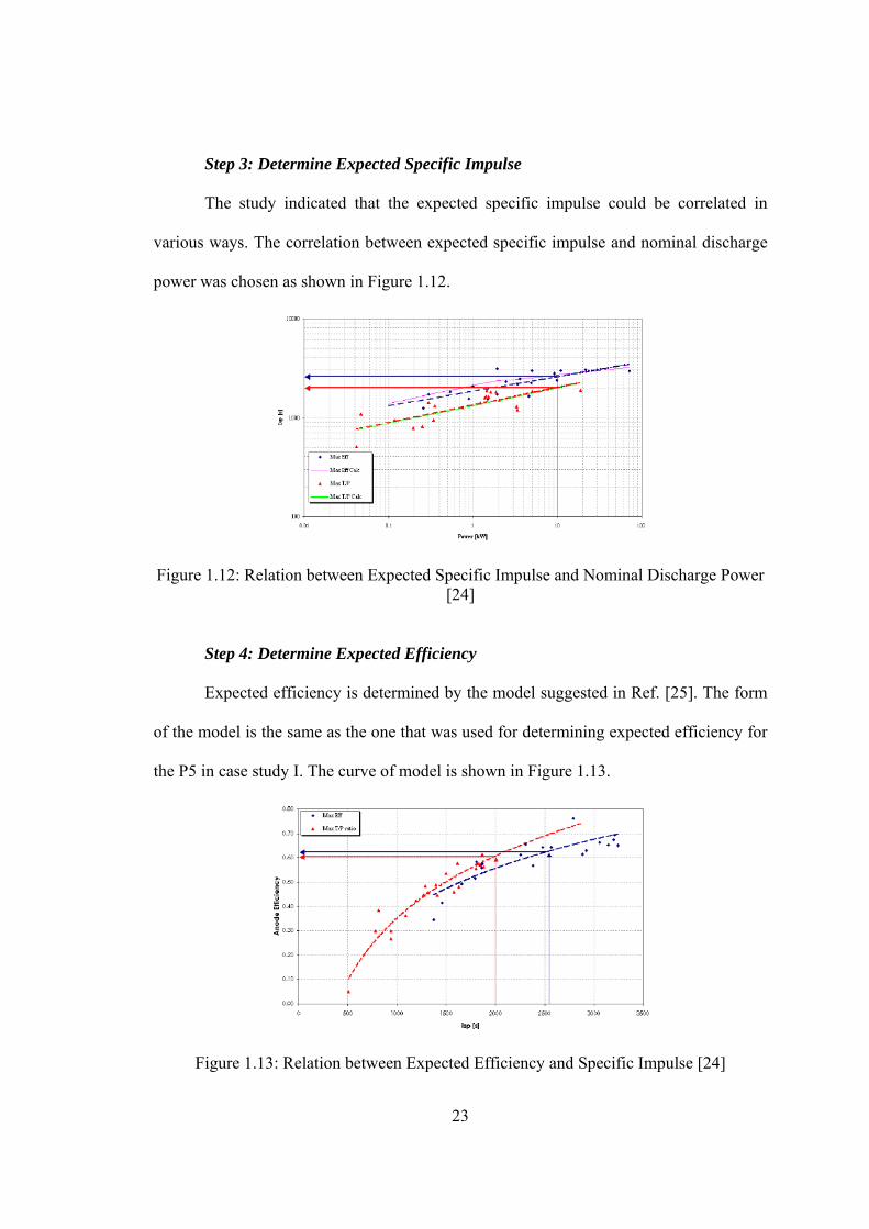
23
Step 3: Determine Expected Specific Impulse
The study indicated that the expected specific impulse could be correlated in
various ways. The correlation between expected specific impulse and nominal discharge
power was chosen as shown in Figure 1.12.
Figure 1.12: Relation between Expected Specific Impulse and Nominal Discharge Power [24]
Step 4: Determine Expected Efficiency
Expected efficiency is determined by the model suggested in Ref. [25]. The form
of the model is the same as the one that was used for determining expected efficiency for
the P5 in case study I. The curve of model is shown in Figure 1.13.
Figure 1.13: Relation between Expected Efficiency and Specific Impulse [24]
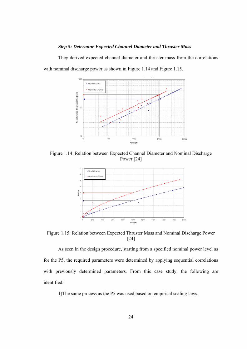
24
Step 5: Determine Expected Channel Diameter and Thruster Mass
They derived expected channel diameter and thruster mass from the correlations
with nominal discharge power as shown in Figure 1.14 and Figure 1.15.
Figure 1.14: Relation between Expected Channel Diameter and Nominal Discharge Power [24]
Figure 1.15: Relation between Expected Thruster Mass and Nominal Discharge Power [24]
As seen in the design procedure, starting from a specified nominal power level as
for the P5, the required parameters were determined by applying sequential correlations
with previously determined parameters. From this case study, the following are
identified:
1)The same process as the P5 was used based on empirical scaling laws.
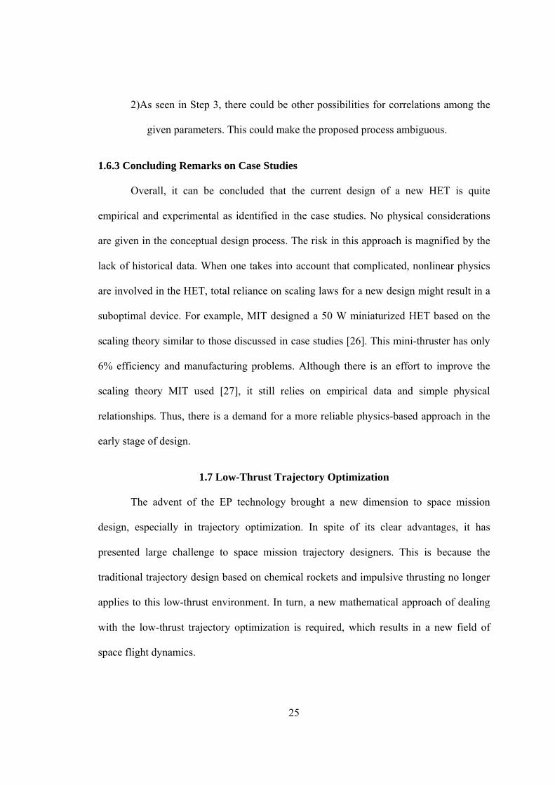
25
2)As seen in Step 3, there could be other possibilities for correlations among the
given parameters. This could make the proposed process ambiguous.
1.6.3 Concluding Remarks on Case Studies
Overall, it can be concluded that the current design of a new HET is quite
empirical and experimental as identified in the case studies. No physical considerations
are given in the conceptual design process. The risk in this approach is magnified by the
lack of historical data. When one takes into account that complicated, nonlinear physics
are involved in the HET, total reliance on scaling laws for a new design might result in a
suboptimal device. For example, MIT designed a 50 W miniaturized HET based on the
scaling theory similar to those discussed in case studies [26]. This mini-thruster has only
6% efficiency and manufacturing problems. Although there is an effort to improve the
scaling theory MIT used [27], it still relies on empirical data and simple physical
relationships. Thus, there is a demand for a more reliable physics-based approach in the
early stage of design.
1.7 Low-Thrust Trajectory Optimization
The advent of the EP technology brought a new dimension to space mission
design, especially in trajectory optimization. In spite of its clear advantages, it has
presented large challenge to space mission trajectory designers. This is because the
traditional trajectory design based on chemical rockets and impulsive thrusting no longer
applies to this low-thrust environment. In turn, a new mathematical approach of dealing
with the low-thrust trajectory optimization is required, which results in a new field of
space flight dynamics.
26
The first realized mission designed by this new method of low-thrust trajectory
optimization was NASA’s Deep Space 1 mission under the NASA New Millennium
Program (NMP) [28]. The goal of this mission was to validate high-risk, advanced
technologies for future missions. The major technology to be validated was Solar Electric
Propulsion (SEP), which was the Ion Propulsion System (IPS) in this specific mission.
The results from this mission were very successful and yielded extensive data which will
be useful for future applications of involved technologies [29]. From a low-thrust
trajectory design perspective, the tools for analyzing low-thrust trajectories were
premature. In addition, there were several challenges in trajectory design with the SEP
compared to conventional trajectory designs using chemical propulsion system; 1) a large
number of unknowns should be determined and a considerable amount of tradeoff studies
should be conducted, 2) spacecraft power consumption is highly coupled with the SEP
thrusting cycle, and 3) spacecraft attitude requirement is also competing with the SEP
thrusting.
Therefore, it is expected that the low-thrust trajectory optimization requires
consistent updates with the spacecraft design evolution. Further sophisticated tools to
optimize the low-thrust trajectory are imperative to handle the large sets of unknown
parameters and properly deal with the unique characteristics of the SEP.
The next mission which successfully applied the SEP was European SMART-1’s
flight to the Moon [30]. In this mission, the HET type of the EP was used rather than the
IPS. Note that the selection of the appropriate electric thrusters largely depends on the
mission requirements and constraints. More sophisticated methods for the low-thrust
trajectory optimization were implemented such as averaging methods, a Finite Element in
27
Time (FET) treatment, and combination of gravity assists and weak stability boundaries
[31]. Since then, a variety of methods for low-thrust trajectory optimization have been
proposed. These methods are well summarized in Ref. [32].
However, all these methods are forced to make assumptions of ideal electric
engines due to difficulties of the problem. The simplest approach is taken to assume that
the EP thrusters have constant efficiency and constant or linear variation of specific
impulse with power. Furthermore, thruster operations at power inputs below the
maximum available power are assumed to be possible, which is not generally true for real
thrusters. Trajectory designers employ the following relations for thrust and mass flow
rate as a function of power given in Equation (1.6) [33].
22 / ( ), 2 / ( )e sp e spT P g I m P g I (1.6)
where, T is the thrust, is the thruster efficiency, P is the required power, m is the
propellant mass flow rate, and spI is the specific impulse. Although there were several
researchers accounting for the variable specific impulse or efficiency, their purposes were
to investigate the effects of its variation on the low-thrust trajectory optimization [34] -
[35]. There was also a demonstration of applying actual thruster performance to the
trajectory optimization, but it employed simple polynomial representations for
performance and mass flow rate variation with power, and did not incorporate a full
operational envelope of the given thruster [36].
Thus, there is also a need to incorporate a more reliable physics-based tool for
performance of electric thrusters in preliminary stage of low-thrust trajectory
optimization.
1.8 Motivation
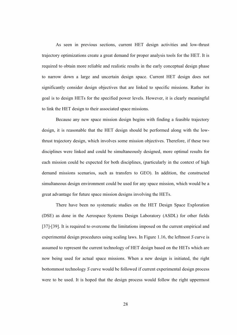
28
As seen in previous sections, current HET design activities and low-thrust
trajectory optimizations create a great demand for proper analysis tools for the HET. It is
required to obtain more reliable and realistic results in the early conceptual design phase
to narrow down a large and uncertain design space. Current HET design does not
significantly consider design objectives that are linked to specific missions. Rather its
goal is to design HETs for the specified power levels. However, it is clearly meaningful
to link the HET design to their associated space missions.
Because any new space mission design begins with finding a feasible trajectory
design, it is reasonable that the HET design should be performed along with the low-
thrust trajectory design, which involves some mission objectives. Therefore, if these two
disciplines were linked and could be simultaneously designed, more optimal results for
each mission could be expected for both disciplines, (particularly in the context of high
demand missions scenarios, such as transfers to GEO). In addition, the constructed
simultaneous design environment could be used for any space mission, which would be a
great advantage for future space mission designs involving the HETs.
There have been no systematic studies on the HET Design Space Exploration
(DSE) as done in the Aerospace Systems Design Laboratory (ASDL) for other fields
[37]-[39]. It is required to overcome the limitations imposed on the current empirical and
experimental design procedures using scaling laws. In Figure 1.16, the leftmost S curve is
assumed to represent the current technology of HET design based on the HETs which are
now being used for actual space missions. When a new design is initiated, the right
bottommost technology S curve would be followed if current experimental design process
were to be used. It is hoped that the design process would follow the right uppermost
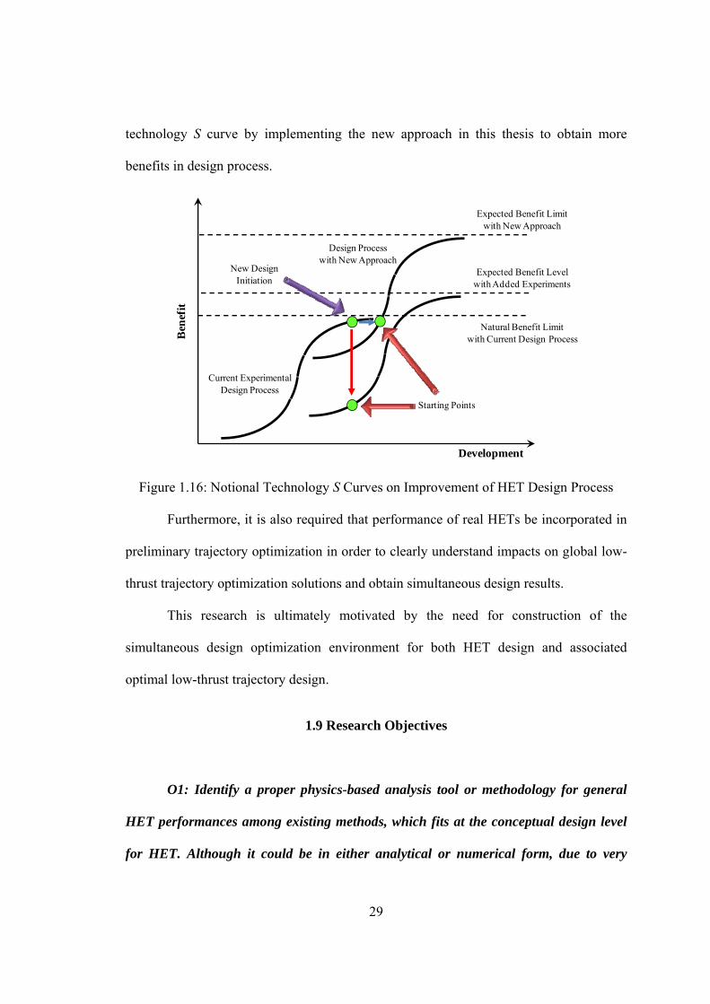
29
technology S curve by implementing the new approach in this thesis to obtain more
benefits in design process.
Development
Ben
efit
Current ExperimentalDesign Process
Design Processwith New Approach
Natural Benefit Limitwith Current Design Process
Expected Benefit Levelwith Added Experiments
Expected Benefit Limitwith New Approach
New DesignInitiation
Starting Points
Figure 1.16: Notional Technology S Curves on Improvement of HET Design Process
Furthermore, it is also required that performance of real HETs be incorporated in
preliminary trajectory optimization in order to clearly understand impacts on global low-
thrust trajectory optimization solutions and obtain simultaneous design results.
This research is ultimately motivated by the need for construction of the
simultaneous design optimization environment for both HET design and associated
optimal low-thrust trajectory design.
1.9 Research Objectives
O1: Identify a proper physics-based analysis tool or methodology for general
HET performances among existing methods, which fits at the conceptual design level
for HET. Although it could be in either analytical or numerical form, due to very
30
complicated and nonlinear physical phenomena in HET, there seems to be no
analytical method. If an adequate tool or methodology were not identified, develop an
appropriate tool or methodology which meets the current research purposes.
O2: Perform conceptual design space exploration for performance metrics with
the identified or developed analysis tool. This task is expected to provide more thorough
information for a new design of HETs in terms of thruster performance. In addition, a
more broad understanding of HET is expected to be gained.
O3: Build the HET performance analysis module based on the identified or
developed HET analysis tool and clearly identify the feasible HET design space for the
simultaneous design optimization with the low-thrust trajectory optimization.
O4: Construct the simultaneous design optimization environment to design a
new HET and associated optimal low-thrust trajectory, which can achieve a specific
space mission objective.
O5: Perform the simultaneous design optimization for a selected space mission
with a specified goal and investigate the optimum solutions. In addition, demonstrate
the capabilities of the simultaneous design optimization environment.
1.10 Research Questions
Based on the motivation, the following research questions arise:

31
UMain Questions
Q1: How can the conceptual design process of HET be improved?
Q2: How can the real thruster performances be infused in preliminary low-
thrust trajectory optimization for a specific space mission?
Q3: How can the simultaneous design optimization environment be
constructed?
USecondary Questions-1
Q4: Can an appropriate physics-based tool or methodology in conceptual level
be found among existing tools or methodologies?
Q5: If not, what is required to develop an appropriate physics-based tool or
methodology?
Q6: In case of developing an appropriate tool, can it be validated for a variety of
existing HETs?
Q7: Can the appropriate tool be efficiently used for the simultaneous design
optimization?
Q8: Can the feasible design space of the HET to be designed be properly
specified for the simultaneous design optimization?
The questions 4 and 8 may be interpreted as those incurred from how the main
questions can be answered.
USecondary Questions-2

32
Q9: What unidentified correlations exist between thruster parameters in terms
of thruster performance metrics?
Q10: Can the existing scaling laws be improved by a physics-based tool or can
new scaling laws be proposed?
Q11: What can be discovered when non-ideal thruster performances are
infused in low-thrust trajectory optimization and what are the differences compared to
that of an ideal one?
The questions 9 through 11 may be interpreted as those incurred from what
contributions can be expected when the main questions are answered.
1.11 Collaboration and Thesis Organization
Based on the research objectives in section 1.9, the current research must cover
three major disciplines such as HET physical analysis, conceptual design methodology
and preliminary low-thrust trajectory optimization. Therefore, it is expected that a great
deal of work would be involved to accomplish the research goals. As a result, it would be
a better approach if the research objectives could be accomplished in collaboration with
people across research laboratories in the Department of Aerospace Engineering at
Georgia Institute of Technology as shown in Figure 1.17.
The issues on HET design and low-thrust trajectory optimization have been
reviewed as well as motivation and corresponding research objectives in this chapter.
Chapter II provides basic materials on mathematical modeling of HET and low-thrust
trajectory optimization to understand the contents of later parts of the thesis. Chapter III
deals with previous research efforts on numerical analysis of HETs. It also provides a
process to identify an appropriate tool among existing tools or methodologies for the
33
current research purpose. Chapter IV details how to develop a new HET analysis tool,
which is a foundation of the thesis. Chapter V gives intensive validation results with the
developed tool. Chapter VI explores the design space of HET using the developed tool.
Chapter VII explains how to build surrogate models for the HET module in a
simultaneous design optimization environment. Chapter VIII culminates the thesis work
by demonstrating the capability of the simultaneous design optimization environment for
a specific space mission. Finally, Chapter IX addresses conclusions of the present
research, contributions, and future work.
Figure 1.17: Collaboration Framework
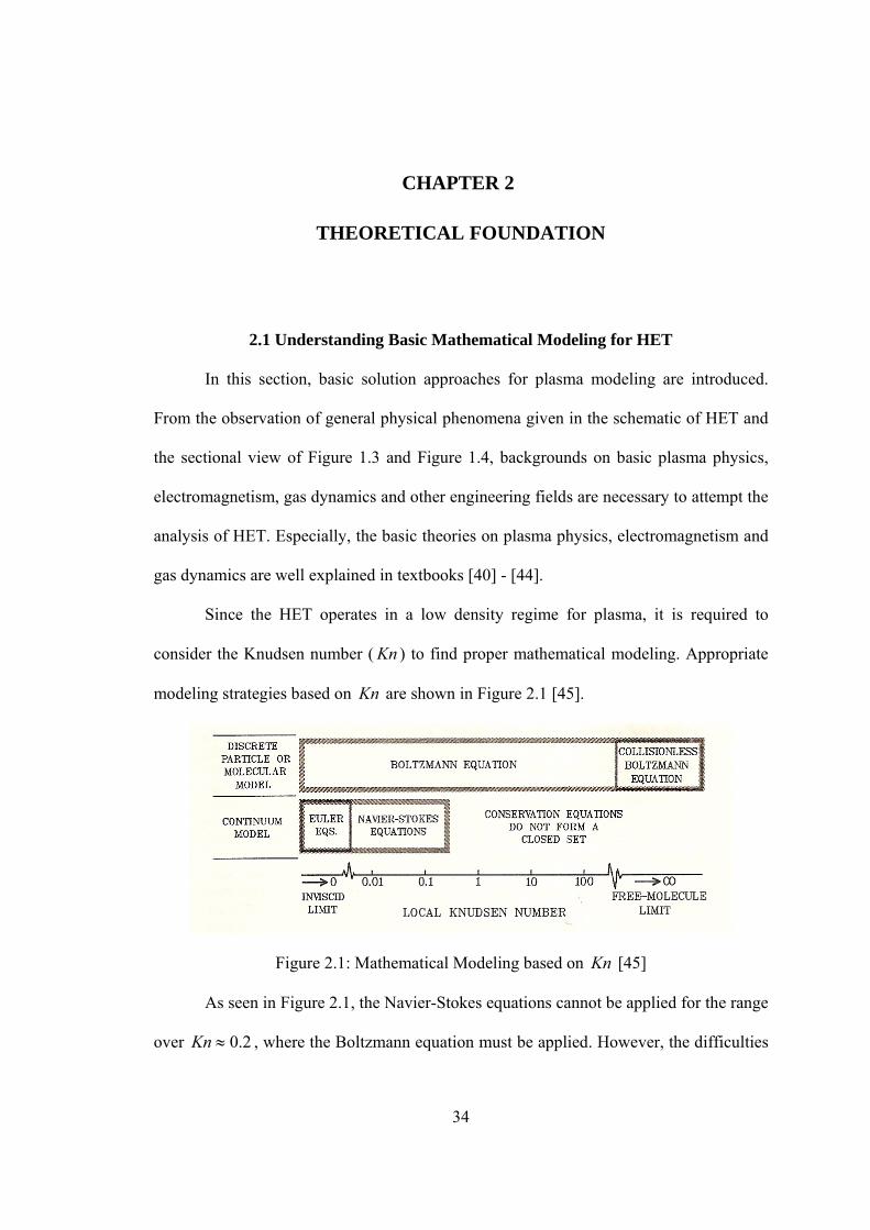
34
CHAPTER 2
THEORETICAL FOUNDATION
2.1 Understanding Basic Mathematical Modeling for HET
In this section, basic solution approaches for plasma modeling are introduced.
From the observation of general physical phenomena given in the schematic of HET and
the sectional view of Figure 1.3 and Figure 1.4, backgrounds on basic plasma physics,
electromagnetism, gas dynamics and other engineering fields are necessary to attempt the
analysis of HET. Especially, the basic theories on plasma physics, electromagnetism and
gas dynamics are well explained in textbooks [40] - [44].
Since the HET operates in a low density regime for plasma, it is required to
consider the Knudsen number ( Kn ) to find proper mathematical modeling. Appropriate
modeling strategies based on Kn are shown in Figure 2.1 [45].
Figure 2.1: Mathematical Modeling based on Kn [45]
As seen in Figure 2.1, the Navier-Stokes equations cannot be applied for the range
over 2.0Kn , where the Boltzmann equation must be applied. However, the difficulties
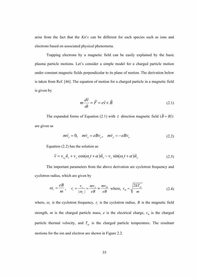
35
arise from the fact that the sKn' can be different for each species such as ions and
electrons based on associated physical phenomena.
Trapping electrons by a magnetic field can be easily explained by the basic
plasma particle motions. Let’s consider a simple model for a charged particle motion
under constant magnetic fields perpendicular to its plane of motion. The derivation below
is taken from Ref. [46]. The equation of motion for a charged particle in a magnetic field
is given by
BveFdt
vdm
(2.1)
The expanded forms of Equation (2.1) with z direction magnetic field )ˆ( zBB
are given as
xyyxz eBvvmeBvvmvm ,,0 (2.2)
Equation (2.2) has the solution as
ycxczz ntvntvnvv
)sin()cos(0
(2.3)
The important parameters from the above derivation are cyclotron frequency and
cyclotron radius, which are given by
m
eBc ,
eB
mv
eB
mvvr th
cc
|| where,
2 cpth
kTv
m (2.4)
where, c is the cyclotron frequency, cr is the cyclotron radius, B is the magnetic field
strength, m is the charged particle mass, e is the electrical charge, thv is the charged
particle thermal velocity, and cpT is the charged particle temperature. The resultant
motions for the ion and electron are shown in Figure 2.2.
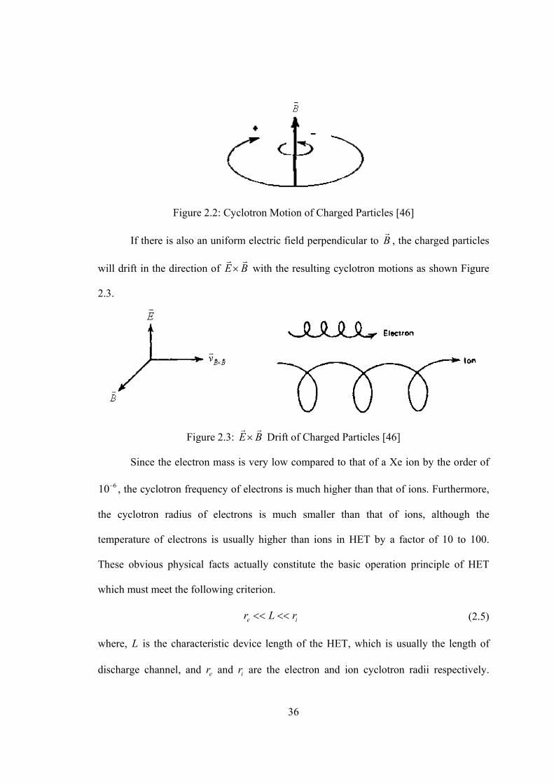
36
Figure 2.2: Cyclotron Motion of Charged Particles [46]
If there is also an uniform electric field perpendicular to B
, the charged particles
will drift in the direction of BE
with the resulting cyclotron motions as shown Figure
2.3.
Figure 2.3: BE
Drift of Charged Particles [46]
Since the electron mass is very low compared to that of a Xe ion by the order of
610 , the cyclotron frequency of electrons is much higher than that of ions. Furthermore,
the cyclotron radius of electrons is much smaller than that of ions, although the
temperature of electrons is usually higher than ions in HET by a factor of 10 to 100.
These obvious physical facts actually constitute the basic operation principle of HET
which must meet the following criterion.
ie rLr (2.5)
where, L is the characteristic device length of the HET, which is usually the length of
discharge channel, and er and ir are the electron and ion cyclotron radii respectively.
37
Equation (2.5) demonstrates that in a conventional HET the electrons are magnetized but
the ions are not. Therefore, the electrons are trapped by the magnetic field for larger
residence times (and more effective ionization) while the ions are not affected by the
magnetic field so that they can be accelerated by the applied electric field.
It is expected that the elections are under high collisional states, but ions are not.
Subsequently, the Kn of electrons is lower than that of ions. Neutrals are also expected
to have higher Kn . Therefore, it seems that the Boltzmann equation should be applied for
the neutrals and ions, and the Navier-Stokes equations can be applied for the electrons,
which considers the bulk of electrons as a continuum fluid.
Considerable technical papers have been published on the numerical methods to
analyze EP devices. The overview on this is well explained in Ref. [47]. The numerical
methods fall in three major categories: kinetic, continuum/fluid, and hybrid method
which combines the first two modeling approaches.
The kinetic modeling has been used for the high Kn regime in which the physical
phenomena are not well represented by the fluid description. This modeling is basically
based on the spirit of solving the Boltzmann equation.
The Boltzmann equation is given by
collt
f
v
f
m
F
x
fv
t
f
(2.6)
where, f is the particle distribution function in phase space, x
is the space coordinate,
v
is the velocity coordinate, F
is the force vector in space coordinate, and colltf / is
the time rate of change of the distribution function by collisions. As seen in Equation
(2.6), although the differential order of the Boltzmann equation is only 1 in all
38
independent variables, t , x
and v
, solving it can be computationally prohibitive for
many body systems and very detailed phase space descriptions. Furthermore, a correct
mathematical representation of colltf / is not available for most physical situations.
For a thermodynamic equilibrium system, colltf / can be considered to be zero. An
electron fluid in an HET is rarely in complete thermodynamic equilibrium.
In order to circumvent this difficulty, scientists and engineers especially in the
nuclear society have developed methods to solve the Boltzmann equation using particles,
i.e., kinetic modeling [48] - [49]. Particle simulations directly deal with particles and
solve each individual particle motion under the given forces. The approach is as follows.
Since the Boltzmann equation with / 0coll
f t merely represents the conservation of
the particle distribution function in the phase space, the particle motion can be easily
solved simply using Newton’s 2 P
ndP law with the exerted forces. Then the integrations will
provide new velocity and new position for each particle. After moving the particles
during a given time step, the collisional effects can be modeled by the collision
probabilities as
colltcoll eP 1 (2.7)
where, collP is the collision probability, t is the time step, and coll is the total collision
frequency. By comparing this probability with a random number, the occurrence of
collision is determined and if a collision occurs, another random number is used to
determine what type of collision it would be. Then the collisional interaction is applied
according to the determined collision type. This way of dealing with the collisions is an
indirect modeling of colltf / . The use of random numbers manifests the Monte Carlo

39
method [50] - [51]. There are various classes of this modeling approach, for example,
Monte Carlo Collision (MCC) and Direct Simulation Monte Carlo (DSMC) [52].
Since this approach directly simulates the particle motions, the computational cost
are very high at every time step. All the particles must be swept to calculate the
interacting forces and collision probabilities. In order to expedite the calculation, nuclear
scientists have developed the concept of Particle-Mesh (PM) model, usually called
Particle-In-Cell (PIC) methodology [49]. In this methodology, the meshes are used to get
macroscopic quantities such as number density, charge density, temperature and so on. In
particular, the charge density is input into the Gauss’ law, which is one of the Maxwell’s
equations, to allow for solving the Poisson’s equation. Thus, forces are obtained from the
resultant field distribution, not the direct calculations by the Coulomb law. In this way,
the computational cost to calculate forces can be significantly reduced. In spite of this
effort at reducing the computational cost, the kinetic modeling is still impractical for the
most HET calculations. There are several factors to make adaption of the kinetic method
impractical such as follows.
1)Although the plasma number density is low ( 31916 /1010 m ) relative to the
general flow problem, it is still too high to directly apply the kinetic method.
It’s obviously impractical to track billions and billions of particles at every
time step using current computer capabilities.
2)What makes matters worse is the time step restriction. In order to resolve
accurate motion of the charged particles, especially electrons, due to their high
40
mobility, the allowable time step is limited by the plasma frequency, which is
one of the basic parameters for plasma and is given by
0
2
m
enop (2.8)
where, p is the plasma frequency, 0n is the plasma number density, e is the
electrical charge, m is the mass of charged particle, and 0 is the freespace
permittivity. Usually the plasma frequency of electrons ( sec/1011 radp )
is higher than that of ions due to smaller mass, which yields the time step on
the order of sec10 11 .
3)Another important plasma parameter also makes the implementation difficult,
the Debye length, which is given by
0
2
p
o
kT
n e
(2.9)
where, is the Debye length, k is the Boltzmann constant, and pT is the
plasma temperature. The Debye length is the length over which the charged
particles are screened out from the electric fields inside the Debye sphere.
This quantity comes from the balance between the energy from electric field
and the thermal energy of charged particles. Since the order of the Debye
length is m , several hundred thousand mesh cells may be required for
practical devices.
41
There are several ways of overcoming these impracticalities [52]. The concept of
the superparticle has been used to overcome the first difficulty. A superparticle represents
many actual particles often up to 81 10 particles per a superparticle and is assumed to
have same properties within a superparticle. The size of a superparticle can be determined
by several factors to reproduce the correct physics such as distribution functions or some
other related reactions. For the HET, the ionization rate is an important factor which must
be reproduced correctly.
For getting around the second and third difficulties, the mass ratio between heavy
particles such as neutrals and ions, and electrons can be adjusted to be lower than the
actual value. In addition, the freespace permittivity can be artificially adjusted to a higher
value, which results in lower plasma frequency and higher Debye length.
As a simulation tool, the kinetic approach can resolve the actual physics of HET,
but it still involves computational inefficiency and in turn becomes unmanageable
without artificial assumptions. In addition, the computational cost can still be very high in
spite of these numerical treatments.
The second approach utilizes the fluid description of plasma. In the view of fluid,
the relevant properties are the macroscopic ones, not the details from the microscopic
view as in kinetic modeling. In the light of complex physics involved in HET, one might
be doubtful that the fluid description could accurately represent the correct physics.
However, if one is concerned only about macroscopic properties and general features of
HET, the fluid approach may be the key.
In the Computational Fluid Dynamics (CFD) and numerical combustion societies,
the Navier-Stokes equations are frequently used to obtain solutions. Especially, in
42
numerical combustion, the source term exists in each species conservation equation to
account for chemical reactions. What is usually assumed is mechanical and thermal
equilibrium, but chemical non-equilibrium for multi-species fluid is allowed, which is
called Local Thermodynamic Equilibrium (LTE). However, from the experimental
results for the HET, the plasma might not be in thermodynamic non-equilibrium. In this
case, the typical Navier-Stokes equations or those with each species conservation
equation incorporating source term cannot be directly applied to the HET. Rather, the
classic way of deriving the governing equations must be used to obtain correct
mathematical interpretations for fluid description. This can be done by taking moments of
the Boltzmann equation in the velocity space. The results of this process produce the
conservation of mass, momentum and energy, respectively based on the order of moment.
The generalized moment equation is given as follows [53].
3( ) ( ) s ss s s s s s vs
s colls
F fn n n v v n d v
t t m t
(2.10)
Depending on the expression of , the following three conservation equations for
fluid description can be obtained.
Mass Conservation: 1
vdt
funn
t collv
ssss
3)()(
(2.11)
where, sn is the number density of species s, su
is the mean velocity, and
vdtfcollv s
3/ is the rate of source generation.
Momentum Conservation: vm
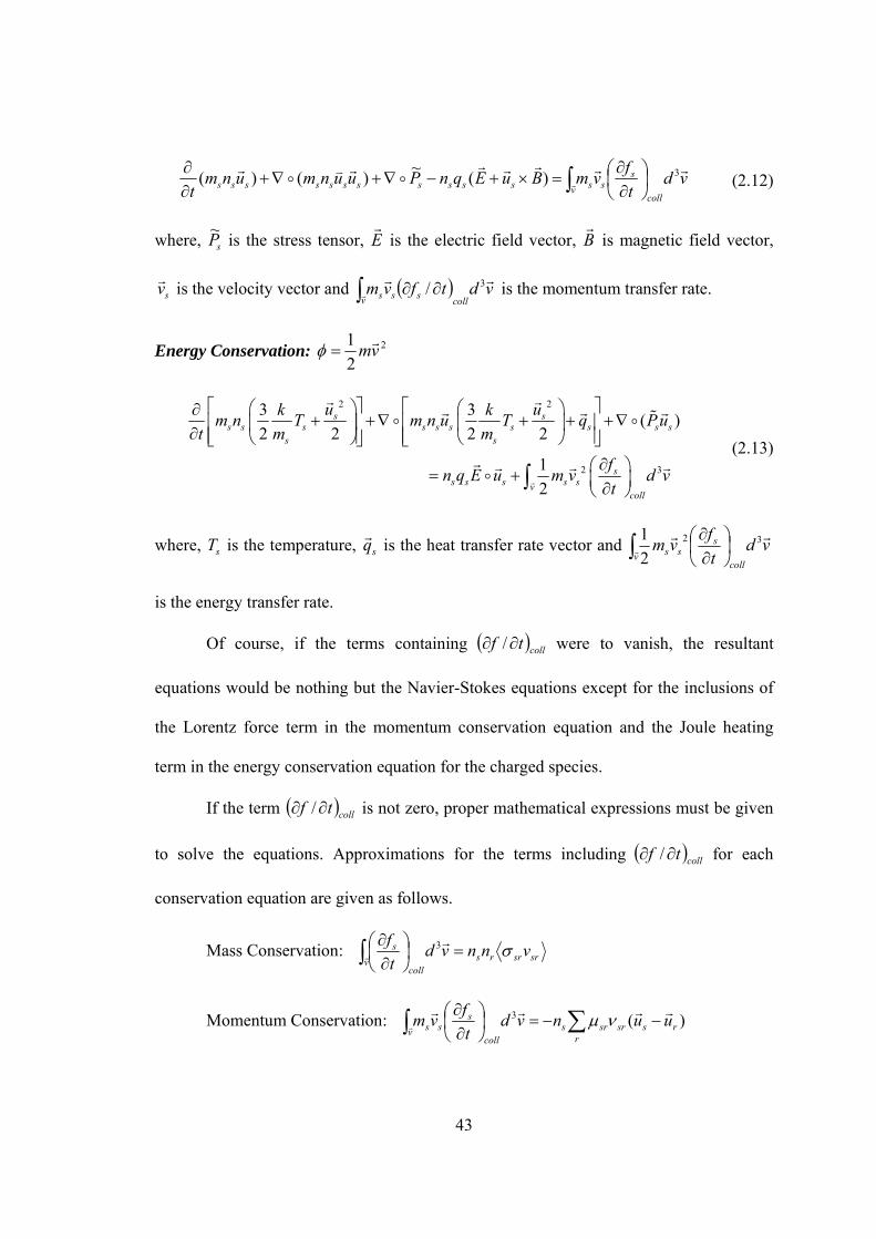
43
vdt
fvmBuEqnPuunmunm
t collv
ssssssssssssss
3)(
~)()(
(2.12)
where, sP~
is the stress tensor, E
is the electric field vector, B
is magnetic field vector,
sv
is the velocity vector and vdtfvmcollv sss
3/ is the momentum transfer rate.
Energy Conservation: 2
2
1vm
2 2
2 3
3 3( )
2 2 2 2
1
2
s ss s s s s s s s s s
s s
ss s s s sv
coll
u uk km n T m n u T q Pu
t m m
fn q E u m v d v
t
(2.13)
where, sT is the temperature, sq
is the heat transfer rate vector and vdt
fvm
collv
sss
32
2
1
is the energy transfer rate.
Of course, if the terms containing colltf / were to vanish, the resultant
equations would be nothing but the Navier-Stokes equations except for the inclusions of
the Lorentz force term in the momentum conservation equation and the Joule heating
term in the energy conservation equation for the charged species.
If the term colltf / is not zero, proper mathematical expressions must be given
to solve the equations. Approximations for the terms including colltf / for each
conservation equation are given as follows.
Mass Conservation: srsrrscoll
v
s vnnvdt
f
3
Momentum Conservation: )(3r
rssrsrs
collv
sss uunvd
t
fvm

44
Energy Conservation:
rsrsrs
collv
sss nvd
t
fvm
32
2
1
where, s represents the concerned species, r represents the species reacting with s species,
sr represents the parameters related to reactions between s and r species, is the cross
section for current reaction, v is the relative velocity between s and r species, is the
reduced mass, is the collision frequency of current reaction, and is the amount of
energy loss required for each reaction. The bracket means the average value.
In order to close the equations, the adequate relations for stress tensor and heat
transfer should also be expressed by other known variables. The collision cross section
for a specific reaction may be obtained from experimental data.
The fluid approach cannot resolve the sheath on a macroscopic scale. The sheath
is the region where quasi-neutrality doesn’t hold. Sheath formation has a very similar
origin in its role to the Debye length previously explained. The sheath plays a role in
producing a smooth transition from the bulk of plasma to the wall. At the edge of the
body of plasma, electrons usually have more mobility than ions by the factor of their
mass ratio. Furthermore, since the electrons have greater temperature than ions, they
move into wall material faster and excess ions are left behind, which results in the
positive charge space. As the electrons which hit the wall reduce the wall potential,
increasing numbers of ions are attracted to the wall. Equilibrium is then attained when the
electron and ion flux going into the wall are exactly the same.
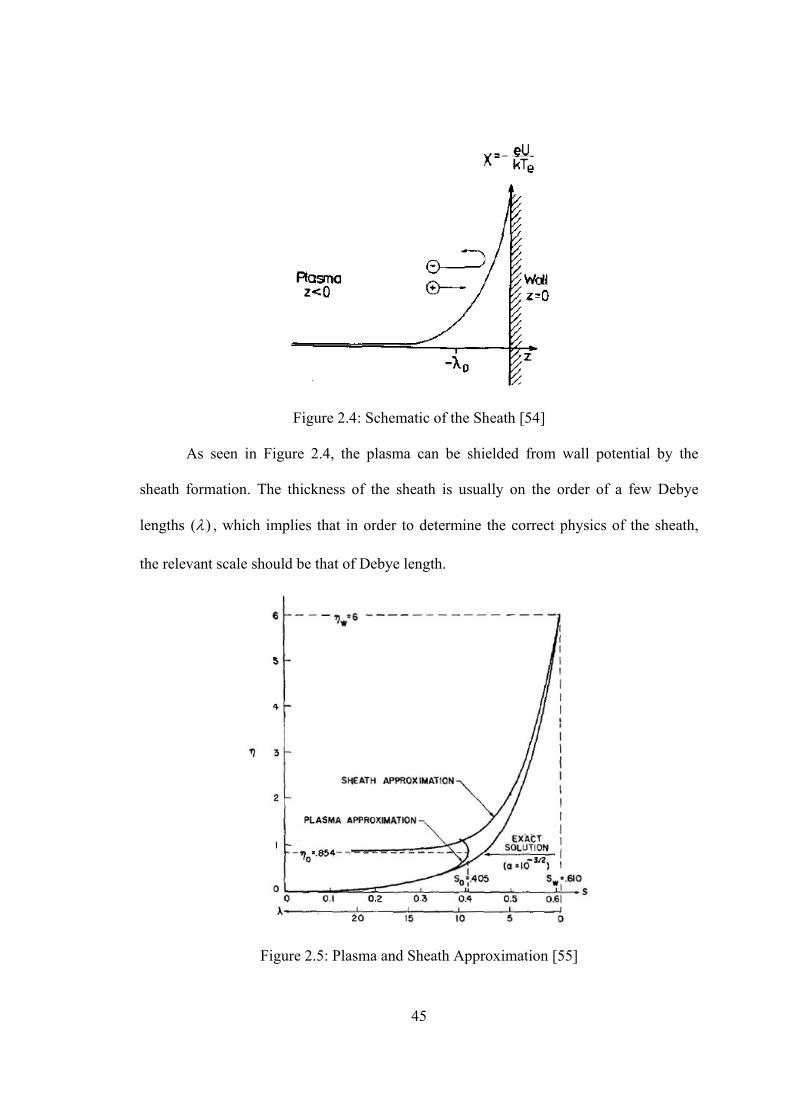
45
Figure 2.4: Schematic of the Sheath [54]
As seen in Figure 2.4, the plasma can be shielded from wall potential by the
sheath formation. The thickness of the sheath is usually on the order of a few Debye
lengths ( ) , which implies that in order to determine the correct physics of the sheath,
the relevant scale should be that of Debye length.
Figure 2.5: Plasma and Sheath Approximation [55]
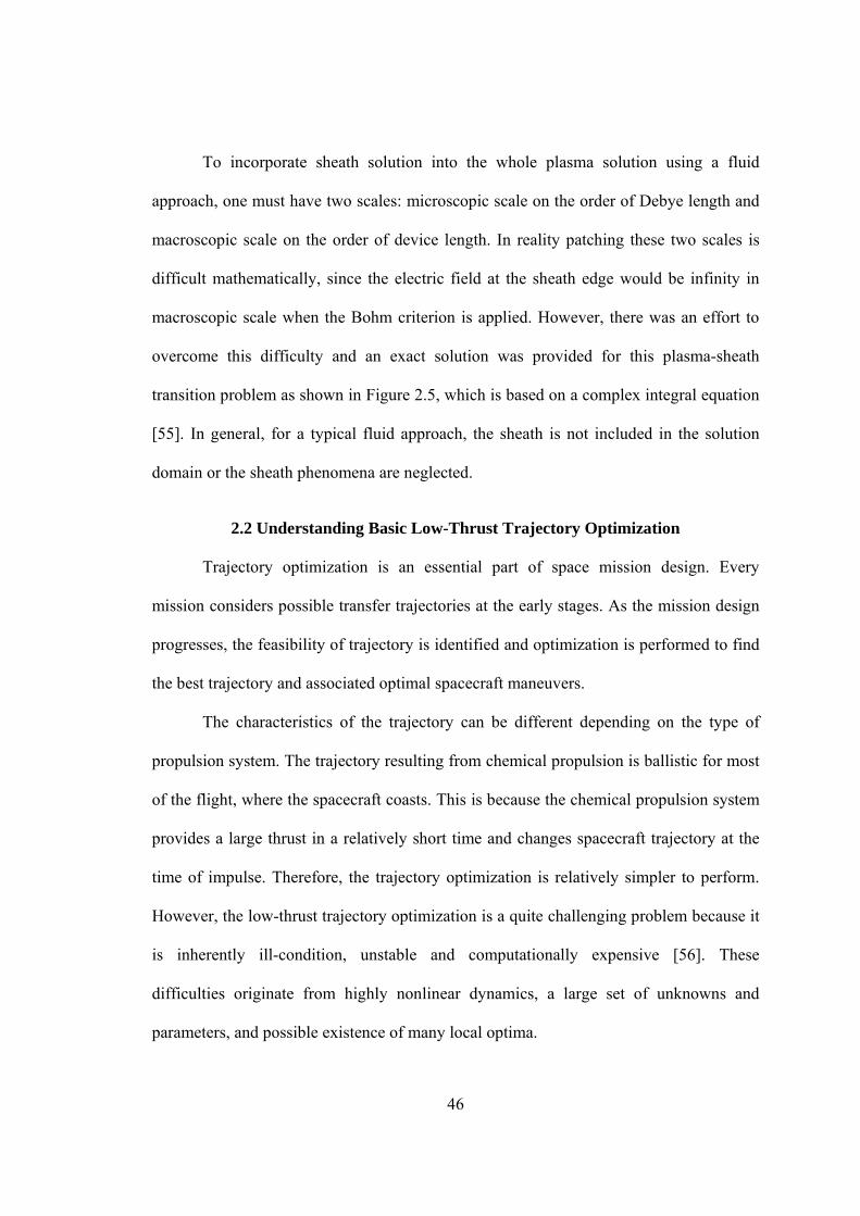
46
To incorporate sheath solution into the whole plasma solution using a fluid
approach, one must have two scales: microscopic scale on the order of Debye length and
macroscopic scale on the order of device length. In reality patching these two scales is
difficult mathematically, since the electric field at the sheath edge would be infinity in
macroscopic scale when the Bohm criterion is applied. However, there was an effort to
overcome this difficulty and an exact solution was provided for this plasma-sheath
transition problem as shown in Figure 2.5, which is based on a complex integral equation
[55]. In general, for a typical fluid approach, the sheath is not included in the solution
domain or the sheath phenomena are neglected.
2.2 Understanding Basic Low-Thrust Trajectory Optimization
Trajectory optimization is an essential part of space mission design. Every
mission considers possible transfer trajectories at the early stages. As the mission design
progresses, the feasibility of trajectory is identified and optimization is performed to find
the best trajectory and associated optimal spacecraft maneuvers.
The characteristics of the trajectory can be different depending on the type of
propulsion system. The trajectory resulting from chemical propulsion is ballistic for most
of the flight, where the spacecraft coasts. This is because the chemical propulsion system
provides a large thrust in a relatively short time and changes spacecraft trajectory at the
time of impulse. Therefore, the trajectory optimization is relatively simpler to perform.
However, the low-thrust trajectory optimization is a quite challenging problem because it
is inherently ill-condition, unstable and computationally expensive [56]. These
difficulties originate from highly nonlinear dynamics, a large set of unknowns and
parameters, and possible existence of many local optima.
47
Because of the considerable advantages of EP, numerous approaches have been
proposed to overcome the aforementioned difficulties. In spite of these efforts,
fundamental difficulties remain. Therefore, the low-thrust trajectory optimization is still
an energetic and evolving field.
In the collaboration framework in this thesis, the low-thrust trajectory
optimization is accomplished by the collaborator. Thus, in this section, basics of the low-
thrust trajectory optimization are reviewed and a brief introduction of a new method
proposed by the collaborator is given.
The methods used for the low-thrust trajectory optimization typically fall under
two categories: indirect and direct methods. The indirect method is original because it is
the same as the one first attempted in typical optimal control theory and it relies on
“Calculus of Variations”. By applying the Pontryagin Maximum Principle [57], the
optimization problem is converted into a Two Point Boundary Value Problem (TPBVP).
In this case, the problem has low-dimension since an infinite dimension control problem
is reduced to a problem calculating “control law”, which is only a function of initial co-
states. Co-states are introduced from Hamiltonian formulation when deriving the
necessary optimality conditions. Although this method is fast, it is very sensitive to initial
guesses of the co-states and difficult to incorporate other constraints such as flybys. In
addition, required boundary conditions must be re-derived for each problem type.
Table 2.1 shows the associated formulation of a continuous nonlinear optimal
controller, which can be used for this problem as well. In Table 2.1, x
is the state vector,
is the co-state vector, is the cost function at the end state, and L is the cost function
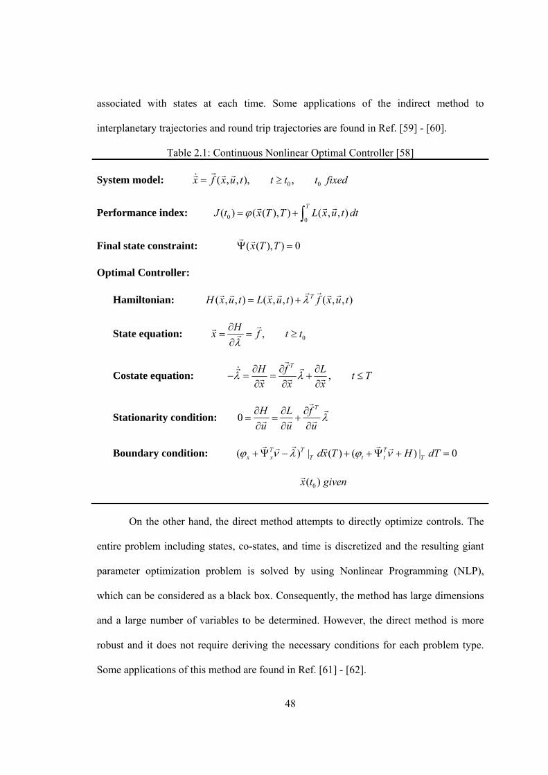
48
associated with states at each time. Some applications of the indirect method to
interplanetary trajectories and round trip trajectories are found in Ref. [59] - [60].
Table 2.1: Continuous Nonlinear Optimal Controller [58]
System model: 0 0( , , ), ,x f x u t t t t fixed
Performance index: 0 0( ) ( ( ), ) ( , , )
TJ t x T T L x u t dt
Final state constraint: ( ( ), ) 0x T T
Optimal Controller:
Hamiltonian: ( , , ) ( , , ) ( , , )TH x u t L x u t f x u t
State equation: 0,H
x f t t
Costate equation: ,TH f L
t Tx x x
Stationarity condition: 0TH L f
u u u
Boundary condition: ( ) | ( ) ( ) | 0T T Tx x T t t Tdx T H dT
0( )x t given
On the other hand, the direct method attempts to directly optimize controls. The
entire problem including states, co-states, and time is discretized and the resulting giant
parameter optimization problem is solved by using Nonlinear Programming (NLP),
which can be considered as a black box. Consequently, the method has large dimensions
and a large number of variables to be determined. However, the direct method is more
robust and it does not require deriving the necessary conditions for each problem type.
Some applications of this method are found in Ref. [61] - [62].
49
Recently, there have been efforts to obtain the advantages of both methods. These
are called hybrid methods which combine the indirect and direct methods. The basic idea
of the hybrid method is that it first uses the direct method to directly minimize some cost,
hit some constraints, and then uses the indirect principles to remove the control
dimensions of the problem. Another idea the collaborator proposed is to use Differential
Dynamic Programming (DDP), which is based on Bellman’s Principle of Optimality of
dynamic programming and successive backward quadratic expansions of the objective
function [63]. By combining DDP with an efficient discretization scheme, improved
convergence properties, and different treatments of hard and soft constraints, he proposed
an efficient Hybrid Differential Dynamic Programming (HDDP) algorithm for low-thrust
trajectory optimization with an emphasis on robustness and flexibility. For more detail
information, refer to Ref. [63].

50
CHAPTER 3
LITERATURE REVIEW AND PHYSICS-BASED ANALYSIS TOOL
IDENTIFICATION FOR HET
3.1 Criteria for Conceptual Physics-Based Analysis Tool for HET
In order to identify a proper physics-based analysis tool or methodology among
existing tools and methodologies for conceptual level design, the following criteria are
proposed:
C1: Numerical Efficiency
Numerical efficiency is apparently the most important property the conceptual
analysis tool must have because a large design space should be explored at the conceptual
level of design.
C2: Numerical Robustness
This criterion is chosen because of the highly complex and nonlinear physics
involved, which may cause unexpected numerical instabilities. Exploring the design
space using a selected tool should be done without execution crash or non-convergence,
which means that the tool should provide solutions for all cases attempted in the design
space, or at least give the criteria on numerically oscillatory cases and physically
impossible cases. In particular, if a tool is highly dependent on the initial guesses, it is not
considered as a robust tool.

51
C3: Self-Consistency
The intended tool should have self-consistency. This criterion is required to cover
an arbitrarily defined design space. In order to meet this criterion, the tool should be as
self-consistent as possible in solution algorithm. In other words, the number of unknowns
which cannot be solved by the tool should be minimized. If this is not the case, the
unknowns must be assigned to some arbitrary values to obtain solution, which results in
the loss of self-consistency.
C4: Physics Representativeness
This criterion is chosen to ensure that the tool should include as much major
physics as possible. The approximate solution provided by the tool should also give
reasonable accuracy at a conceptual level.
UAmong the 4 criteria, the requirements for the first three should be high.
Moderate requirement for the fourth criterion should be enough at the conceptual level
of design.
3.2 Previous Work on HET Numerical Modeling
3.2.1 Full Kinetic Modeling
Several researchers have attempted this modeling approach to simulate HET.
Latocha et al. investigated electron transport in the channel region using PIC-MCC
method [64]. Due to inherent computational inefficiency of the kinetic model, they
proposed an electron diffusion model and compared it with a kinetic model.
52
Adam et al. applied 2D ),( z full kinetic model to HET [65]. Since their research
focus was axial electron transport, no detailed wall effect was included in the domain.
Nonetheless, the model is self-consistent and critical physical information could be
obtained. The average computational time was a month, which is quite expensive. In
order to reduce the constraints on time step and grid spacing, they took cyclotron
frequency and radius as constraints, although the plasma frequency and the Debye length
should be applied to determine time step and grid spacing respectively. This resulted in a
100 times greater time step than that from the plasma frequency constraint.
Taccogna et al. developed 2D Vzr 3),( axisymmetric PIC-MCC program for
HET [66]. They used artificial heavy particle-electron mass ratio and permittivity ratio to
reduce computational cost. They utilized geometrical scaling to lessen computational
loads further while maintaining important physical characteristics. Especially, the model
revealed the existence of the anode sheath and backflow of ions.
The kinetic model can provide detail physics of HET such as electron distribution
function, sheath characteristics, even startup transient characteristics [67] and so on. This
modeling approach is expected to show its capability to gain deeper knowledge of
physics involved in HET. However, it still has a critical drawback in terms of
computational cost even in the current high computer capability environment.
3.2.2 Hybrid Modeling
Hybrid modeling often assumes electrons as a fluid in HET. The first successful
implementation of this approach is attributed to Fife [68] - [69]. He applied PIC-MCC
modeling to ions and neutrals and solved fluid equations to calculate electron temperature.
This method can reduce much of computational cost which was a major obstacle in the
53
kinetic approach. Since the constraints on time step and grid spacing often come from
electron analysis in the kinetic method, if electrons can be treated as fluids, these
constraints are basically eliminated. Several researchers simulated HET with a similar
approach to that of Fife’s method [70] - [72].
However, in spite of the elimination of constraints on time step and grid spacing,
this method still suffers from computational inefficiency due to inherent multiple time
scale problem of HET. In this method, the time step can be taken as those of ions or
neutrals. But, the converged solutions of electron properties must be obtained at every ion
and neutral sweep, which also needs considerable computational time.
3.2.3 Full Fluid Modeling
Various researchers have attempted this approach to investigate macroscopic
behaviors of HET. In this modeling, all the species are modeled as fluids. From the
moments of the Boltzmann equation, mass, momentum and energy conservation
equations are obtained. Quasi-neutrality is often assumed and the simplest approach using
this method is to take steady state forms of the governing equations and construct a
system of ordinary differential equations (ODEs) for dependent variables. The solution
domain is usually taken from anode sheath edge to channel exit or cathode or even a
farther distance. As explained in section 2.2, to also solve for the anode sheath solution,
additional effort and computational cost must be incurred. Currently none of previous
methodologies using fluid approach have attempted to include the anode sheath solution.
The most prominent work on solving a system of ODEs is those of Ahedo et al.
[73] - [78]. They included the boundary condition at the anode sheath and ion backflow
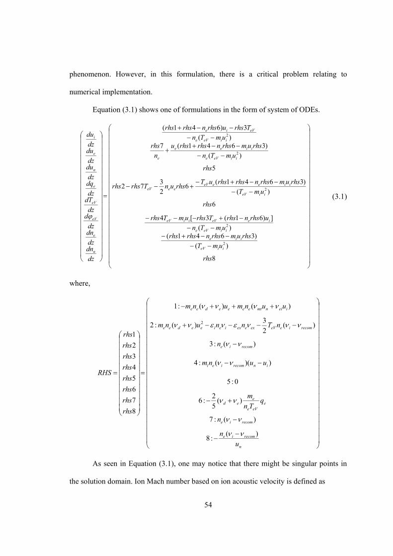
54
phenomenon. However, in this formulation, there is a critical problem relating to
numerical implementation.
Equation (3.1) shows one of formulations in the form of system of ODEs.
8
)(
)3641()(
])61(3[4
6
)(
)3641(6
2
372
5
)(
)3641(7)(
3)641(
2
2
2
2
2
rhs
umT
rhsumrhsnrhsrhsumTn
urhsnrhsTrhsumTrhs
rhs
umT
rhsumrhsnrhsrhsuTrhsunTrhsrhs
rhs
umTn
rhsumrhsnrhsrhsu
n
rhsumTn
Trhsurhsnrhsrhs
dz
dndz
dndz
ddz
dTdz
dqdz
dudz
dudz
du
iieV
iie
iieVe
ieeViieV
iieV
iieeeVeeeV
iieVe
iiee
e
iieVe
eVie
n
e
eV
eV
e
n
e
i
(3.1)
where,
n
recomie
recomie
eeVe
eed
inrecomiei
recomie
recomieeVexeexieieedee
ieinmteeeedee
u
n
n
qTn
m
uunm
n
nTnnunm
uunmunm
rhs
rhs
rhs
rhs
rhs
rhs
rhs
rhs
RHS
)(:8
)(:7
)(5
2:6
0:5
))((:4
)(:3
)(2
3)(:2
)()(:1
8
7
6
5
4
3
2
1
2
As seen in Equation (3.1), one may notice that there might be singular points in
the solution domain. Ion Mach number based on ion acoustic velocity is defined as
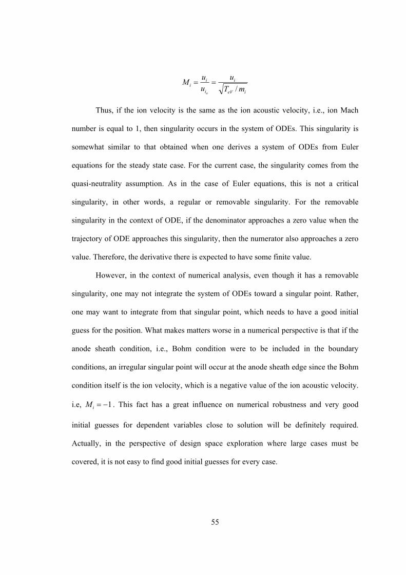
55
ieV
i
i
ii
mT
u
u
uM
a/
Thus, if the ion velocity is the same as the ion acoustic velocity, i.e., ion Mach
number is equal to 1, then singularity occurs in the system of ODEs. This singularity is
somewhat similar to that obtained when one derives a system of ODEs from Euler
equations for the steady state case. For the current case, the singularity comes from the
quasi-neutrality assumption. As in the case of Euler equations, this is not a critical
singularity, in other words, a regular or removable singularity. For the removable
singularity in the context of ODE, if the denominator approaches a zero value when the
trajectory of ODE approaches this singularity, then the numerator also approaches a zero
value. Therefore, the derivative there is expected to have some finite value.
However, in the context of numerical analysis, even though it has a removable
singularity, one may not integrate the system of ODEs toward a singular point. Rather,
one may want to integrate from that singular point, which needs to have a good initial
guess for the position. What makes matters worse in a numerical perspective is that if the
anode sheath condition, i.e., Bohm condition were to be included in the boundary
conditions, an irregular singular point will occur at the anode sheath edge since the Bohm
condition itself is the ion velocity, which is a negative value of the ion acoustic velocity.
i.e, 1iM . This fact has a great influence on numerical robustness and very good
initial guesses for dependent variables close to solution will be definitely required.
Actually, in the perspective of design space exploration where large cases must be
covered, it is not easy to find good initial guesses for every case.
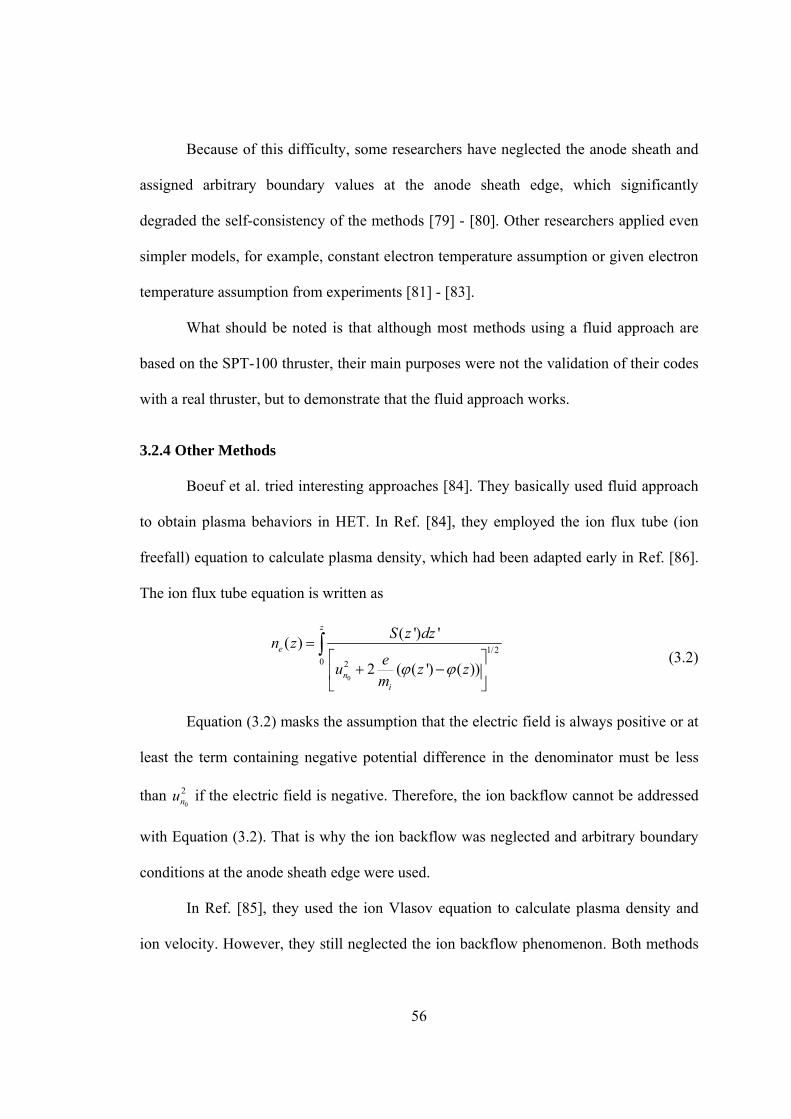
56
Because of this difficulty, some researchers have neglected the anode sheath and
assigned arbitrary boundary values at the anode sheath edge, which significantly
degraded the self-consistency of the methods [79] - [80]. Other researchers applied even
simpler models, for example, constant electron temperature assumption or given electron
temperature assumption from experiments [81] - [83].
What should be noted is that although most methods using a fluid approach are
based on the SPT-100 thruster, their main purposes were not the validation of their codes
with a real thruster, but to demonstrate that the fluid approach works.
3.2.4 Other Methods
Boeuf et al. tried interesting approaches [84]. They basically used fluid approach
to obtain plasma behaviors in HET. In Ref. [84], they employed the ion flux tube (ion
freefall) equation to calculate plasma density, which had been adapted early in Ref. [86].
The ion flux tube equation is written as
0
1/20 2
( ') '( )
2 ( ( ') ( ))
z
e
ni
S z dzn z
eu z z
m
(3.2)
Equation (3.2) masks the assumption that the electric field is always positive or at
least the term containing negative potential difference in the denominator must be less
than 2
0nu if the electric field is negative. Therefore, the ion backflow cannot be addressed
with Equation (3.2). That is why the ion backflow was neglected and arbitrary boundary
conditions at the anode sheath edge were used.
In Ref. [85], they used the ion Vlasov equation to calculate plasma density and
ion velocity. However, they still neglected the ion backflow phenomenon. Both methods
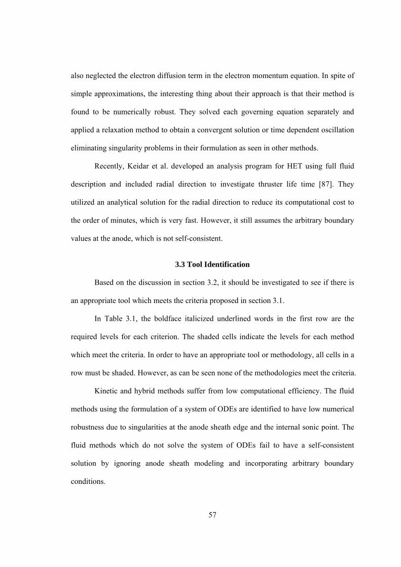
57
also neglected the electron diffusion term in the electron momentum equation. In spite of
simple approximations, the interesting thing about their approach is that their method is
found to be numerically robust. They solved each governing equation separately and
applied a relaxation method to obtain a convergent solution or time dependent oscillation
eliminating singularity problems in their formulation as seen in other methods.
Recently, Keidar et al. developed an analysis program for HET using full fluid
description and included radial direction to investigate thruster life time [87]. They
utilized an analytical solution for the radial direction to reduce its computational cost to
the order of minutes, which is very fast. However, it still assumes the arbitrary boundary
values at the anode, which is not self-consistent.
3.3 Tool Identification
Based on the discussion in section 3.2, it should be investigated to see if there is
an appropriate tool which meets the criteria proposed in section 3.1.
In Table 3.1, the boldface italicized underlined words in the first row are the
required levels for each criterion. The shaded cells indicate the levels for each method
which meet the criteria. In order to have an appropriate tool or methodology, all cells in a
row must be shaded. However, as can be seen none of the methodologies meet the criteria.
Kinetic and hybrid methods suffer from low computational efficiency. The fluid
methods using the formulation of a system of ODEs are identified to have low numerical
robustness due to singularities at the anode sheath edge and the internal sonic point. The
fluid methods which do not solve the system of ODEs fail to have a self-consistent
solution by ignoring anode sheath modeling and incorporating arbitrary boundary
conditions.
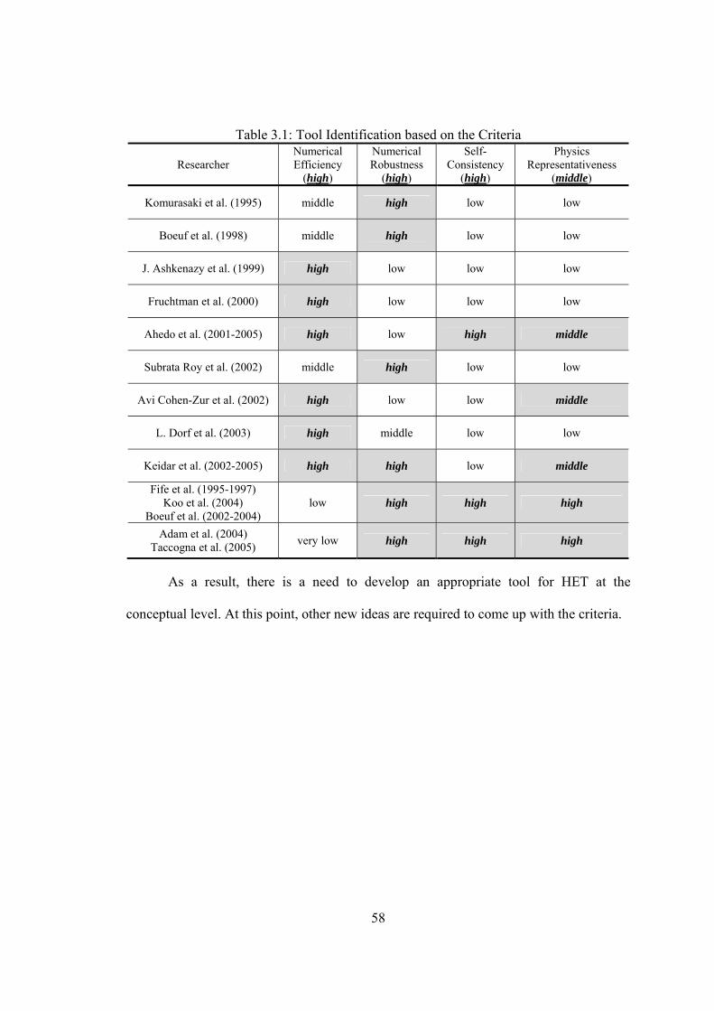
58
Table 3.1: Tool Identification based on the Criteria
Researcher Numerical Efficiency
(Uhigh U)
Numerical Robustness
(UhighU)
Self-Consistency
(UhighU)
Physics Representativeness
(Umiddle U)
Komurasaki et al. (1995) middle high low low
Boeuf et al. (1998) middle high low low
J. Ashkenazy et al. (1999) high low low low
Fruchtman et al. (2000) high low low low
Ahedo et al. (2001-2005) high low high middle
Subrata Roy et al. (2002) middle high low low
Avi Cohen-Zur et al. (2002) high low low middle
L. Dorf et al. (2003) high middle low low
Keidar et al. (2002-2005) high high low middle
Fife et al. (1995-1997) Koo et al. (2004)
Boeuf et al. (2002-2004) low high high high
Adam et al. (2004) Taccogna et al. (2005)
very low high high high
As a result, there is a need to develop an appropriate tool for HET at the
conceptual level. At this point, other new ideas are required to come up with the criteria.

59
CHAPTER 4
PHYSICS-BASED ANALYSIS TOOL DEVELOPMENT FOR HET
4.1 Hypotheses for an Intended Tool
In order to develop an appropriate tool, the following hypotheses are proposed.
UHypothesis 1
If the highly detail physics can be properly omitted when providing macroscopic
performance metrics, the fluid approach will be a good candidate for improving
numerical efficiency.
UHypothesis 2
If the singular form of a system of ODEs occurring in fluid approach can be
avoided somehow, numerical robustness will be improved.
UHypothesis 3
If proper modeling near the anode region is included in the fluid approach, a self-
consistent model will be constructed and the number of arbitrary boundary conditions
will be reduced.
UHypothesis 4
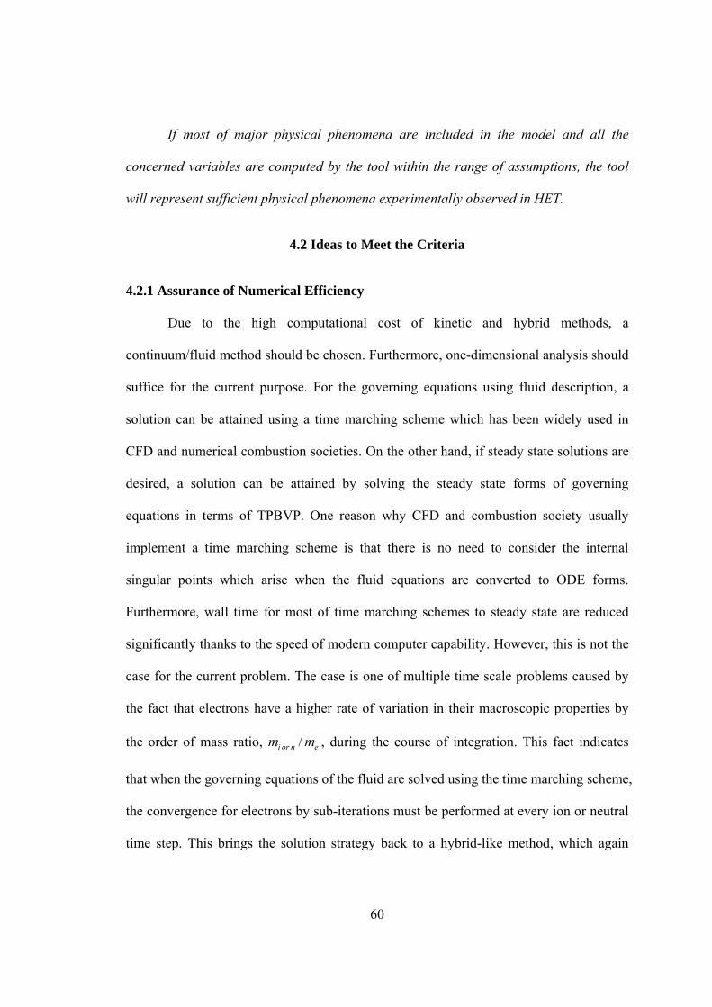
60
If most of major physical phenomena are included in the model and all the
concerned variables are computed by the tool within the range of assumptions, the tool
will represent sufficient physical phenomena experimentally observed in HET.
4.2 Ideas to Meet the Criteria
4.2.1 Assurance of Numerical Efficiency
Due to the high computational cost of kinetic and hybrid methods, a
continuum/fluid method should be chosen. Furthermore, one-dimensional analysis should
suffice for the current purpose. For the governing equations using fluid description, a
solution can be attained using a time marching scheme which has been widely used in
CFD and numerical combustion societies. On the other hand, if steady state solutions are
desired, a solution can be attained by solving the steady state forms of governing
equations in terms of TPBVP. One reason why CFD and combustion society usually
implement a time marching scheme is that there is no need to consider the internal
singular points which arise when the fluid equations are converted to ODE forms.
Furthermore, wall time for most of time marching schemes to steady state are reduced
significantly thanks to the speed of modern computer capability. However, this is not the
case for the current problem. The case is one of multiple time scale problems caused by
the fact that electrons have a higher rate of variation in their macroscopic properties by
the order of mass ratio, enori mm / , during the course of integration. This fact indicates
that when the governing equations of the fluid are solved using the time marching scheme,
the convergence for electrons by sub-iterations must be performed at every ion or neutral
time step. This brings the solution strategy back to a hybrid-like method, which again
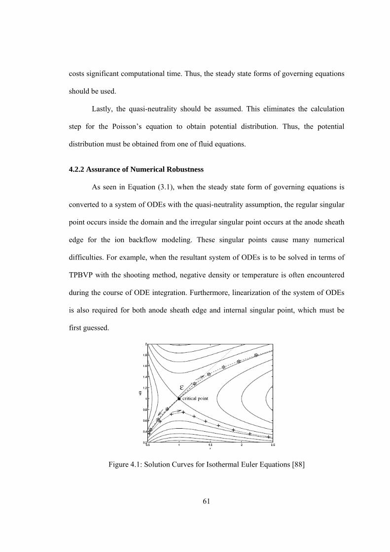
61
costs significant computational time. Thus, the steady state forms of governing equations
should be used.
Lastly, the quasi-neutrality should be assumed. This eliminates the calculation
step for the Poisson’s equation to obtain potential distribution. Thus, the potential
distribution must be obtained from one of fluid equations.
4.2.2 Assurance of Numerical Robustness
As seen in Equation (3.1), when the steady state form of governing equations is
converted to a system of ODEs with the quasi-neutrality assumption, the regular singular
point occurs inside the domain and the irregular singular point occurs at the anode sheath
edge for the ion backflow modeling. These singular points cause many numerical
difficulties. For example, when the resultant system of ODEs is to be solved in terms of
TPBVP with the shooting method, negative density or temperature is often encountered
during the course of ODE integration. Furthermore, linearization of the system of ODEs
is also required for both anode sheath edge and internal singular point, which must be
first guessed.
Figure 4.1: Solution Curves for Isothermal Euler Equations [88]
62
The linearization near the internal singular point is required to have a higher
accuracy since this kind of removable singularity usually has a unique solution as in
subsonic-supersonic transition flow, which is shown in Figure 4.1. Although a new
method using dynamical system formulation to deal with this problem was suggested
recently [88], it still requires very good initial guesses for dependent variables and
internal singular point location.
Actually, the shooting method is not good for highly nonlinear problems due to
breakdown of the code in the course of integration by previously stated reasons. One can
think of other methods like multiple shooting [89] or finite difference method [90]. These
methods divide the domain into smaller sub-intervals and integrations are performed on
each interval. Then the values at each interface between sub-intervals are matched by
Newton’s method. However, other problems still exist if the singular forms of ODEs are
maintained. Multiple shooting method makes the problem more difficult to solve. Since
the location of internal singular point is not known in advance, a numerical treatment of
moving the internal singular point from one sub-interval to another is definitely required,
which might cause slow convergence. Although a finite difference method can deal with
the internal singular point by adaptive grid strategy, it still has numerical instability such
as gradient blow-up in the vicinity of an internal singular point with poor initial
conditions. As a result, the strategy of solving the system of ODEs with a quasi-neutrality
assumption should be avoided and a more robust strategy should be found.
In order to avoid the singular formulation, each ODE for a specific variable can
be solved sequentially while other variables remain constant. Then the convergence can
be obtained by iterations. This is the same method of the so called fixed point iteration in
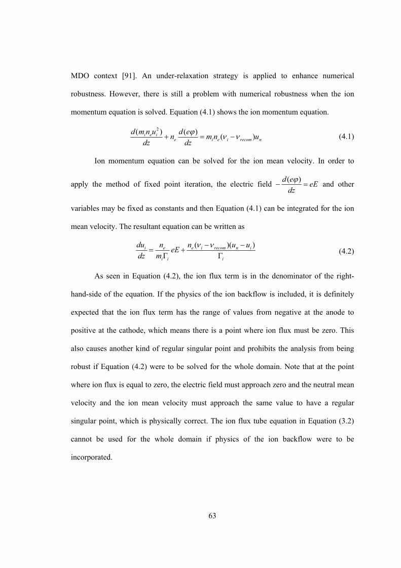
63
MDO context [91]. An under-relaxation strategy is applied to enhance numerical
robustness. However, there is still a problem with numerical robustness when the ion
momentum equation is solved. Equation (4.1) shows the ion momentum equation.
nrecomieieiei unm
dz
edn
dz
unmd)(
)()( 2
(4.1)
Ion momentum equation can be solved for the ion mean velocity. In order to
apply the method of fixed point iteration, the electric field eEdz
ed
)( and other
variables may be fixed as constants and then Equation (4.1) can be integrated for the ion
mean velocity. The resultant equation can be written as
i
inrecomie
ii
ei uuneE
m
n
dz
du
))((
(4.2)
As seen in Equation (4.2), the ion flux term is in the denominator of the right-
hand-side of the equation. If the physics of the ion backflow is included, it is definitely
expected that the ion flux term has the range of values from negative at the anode to
positive at the cathode, which means there is a point where ion flux must be zero. This
also causes another kind of regular singular point and prohibits the analysis from being
robust if Equation (4.2) were to be solved for the whole domain. Note that at the point
where ion flux is equal to zero, the electric field must approach zero and the neutral mean
velocity and the ion mean velocity must approach the same value to have a regular
singular point, which is physically correct. The ion flux tube equation in Equation (3.2)
cannot be used for the whole domain if physics of the ion backflow were to be
incorporated.
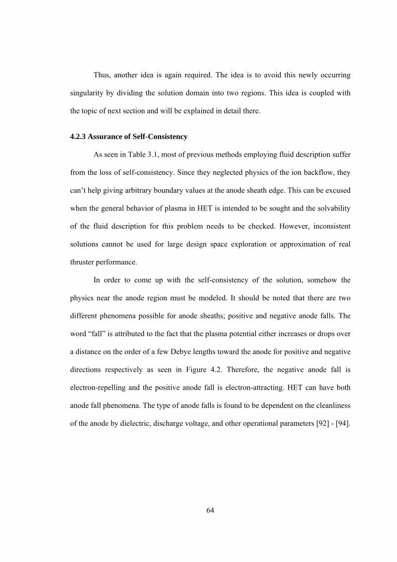
64
Thus, another idea is again required. The idea is to avoid this newly occurring
singularity by dividing the solution domain into two regions. This idea is coupled with
the topic of next section and will be explained in detail there.
4.2.3 Assurance of Self-Consistency
As seen in Table 3.1, most of previous methods employing fluid description suffer
from the loss of self-consistency. Since they neglected physics of the ion backflow, they
can’t help giving arbitrary boundary values at the anode sheath edge. This can be excused
when the general behavior of plasma in HET is intended to be sought and the solvability
of the fluid description for this problem needs to be checked. However, inconsistent
solutions cannot be used for large design space exploration or approximation of real
thruster performance.
In order to come up with the self-consistency of the solution, somehow the
physics near the anode region must be modeled. It should be noted that there are two
different phenomena possible for anode sheaths; positive and negative anode falls. The
word “fall” is attributed to the fact that the plasma potential either increases or drops over
a distance on the order of a few Debye lengths toward the anode for positive and negative
directions respectively as seen in Figure 4.2. Therefore, the negative anode fall is
electron-repelling and the positive anode fall is electron-attracting. HET can have both
anode fall phenomena. The type of anode falls is found to be dependent on the cleanliness
of the anode by dielectric, discharge voltage, and other operational parameters [92] - [94].
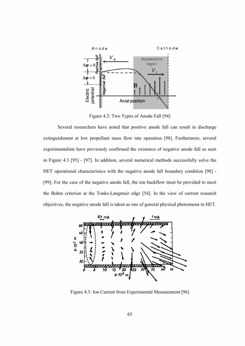
65
Figure 4.2: Two Types of Anode Fall [94]
Several researchers have noted that positive anode fall can result in discharge
extinguishment at low propellant mass flow rate operation [98]. Furthermore, several
experimentalists have previously confirmed the existence of negative anode fall as seen
in Figure 4.3 [95] - [97]. In addition, several numerical methods successfully solve the
HET operational characteristics with the negative anode fall boundary condition [98] -
[99]. For the case of the negative anode fall, the ion backflow must be provided to meet
the Bohm criterion at the Tonks-Langmuir edge [54]. In the view of current research
objectives, the negative anode fall is taken as one of general physical phenomena in HET.
Figure 4.3: Ion Current from Experimental Measurement [96]
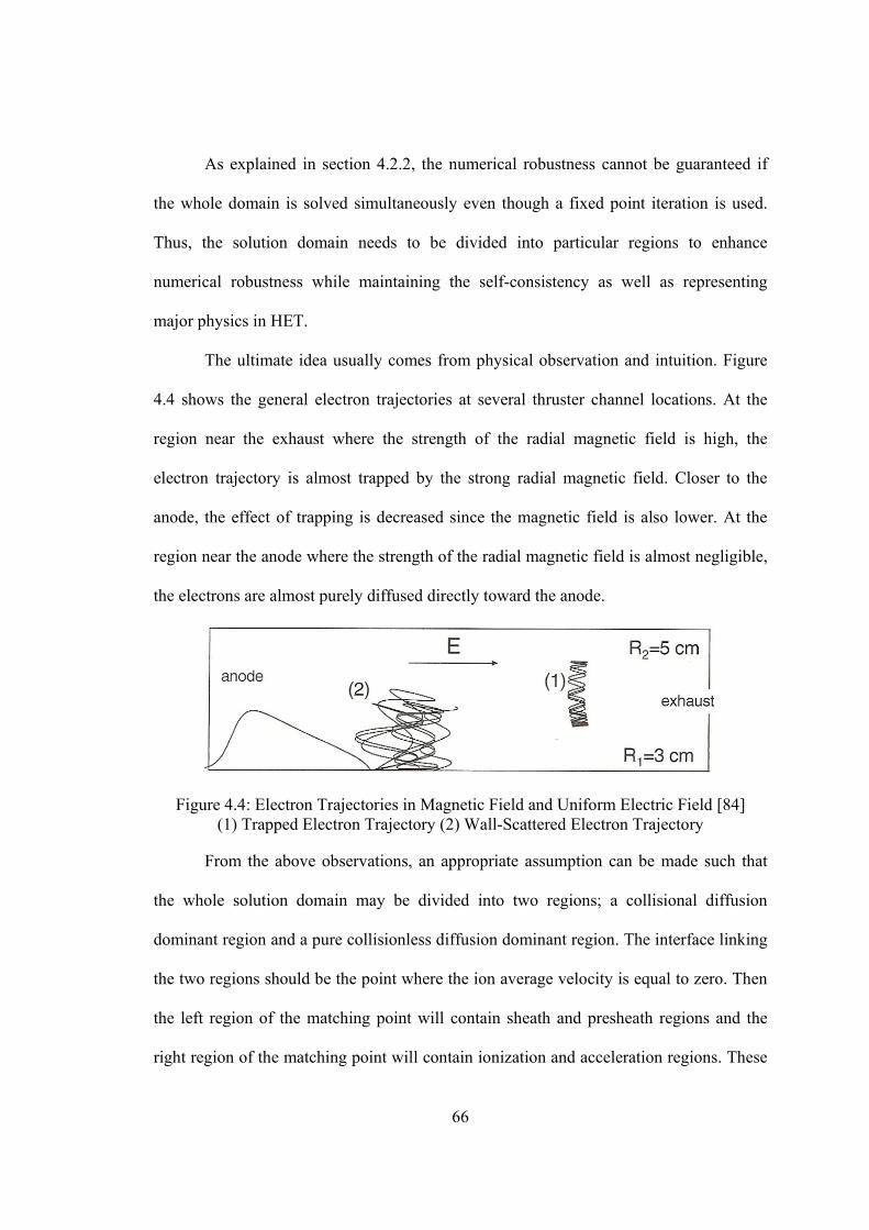
66
As explained in section 4.2.2, the numerical robustness cannot be guaranteed if
the whole domain is solved simultaneously even though a fixed point iteration is used.
Thus, the solution domain needs to be divided into particular regions to enhance
numerical robustness while maintaining the self-consistency as well as representing
major physics in HET.
The ultimate idea usually comes from physical observation and intuition. Figure
4.4 shows the general electron trajectories at several thruster channel locations. At the
region near the exhaust where the strength of the radial magnetic field is high, the
electron trajectory is almost trapped by the strong radial magnetic field. Closer to the
anode, the effect of trapping is decreased since the magnetic field is also lower. At the
region near the anode where the strength of the radial magnetic field is almost negligible,
the electrons are almost purely diffused directly toward the anode.
Figure 4.4: Electron Trajectories in Magnetic Field and Uniform Electric Field [84] (1) Trapped Electron Trajectory (2) Wall-Scattered Electron Trajectory
From the above observations, an appropriate assumption can be made such that
the whole solution domain may be divided into two regions; a collisional diffusion
dominant region and a pure collisionless diffusion dominant region. The interface linking
the two regions should be the point where the ion average velocity is equal to zero. Then
the left region of the matching point will contain sheath and presheath regions and the
right region of the matching point will contain ionization and acceleration regions. These
67
two regions are mathematically distinguished mainly by different treatments of the
electron momentum equation. The electron momentum equation can be simplified with
the assumptions of steady state, neglecting electron inertia terms, reducing stress tensor to
pure pressure, and neglecting mean velocities of other species compared to the much
higher electron mean velocity. In addition, the azimuthal electron mean velocity obtained
from stochastic analysis through the Langevin equation (Appendix A) can be substituted.
The resultant equation of these simplifications and substitution is given by Equation (4.3).
2
, 2,
( ) ( )0 1e e e
e e e e eff ee eff
d n kT d en m n u
dz dz
(4.3)
Equation (4.3) is actually one type of Ohm’s law. This equation is reduced to the
different forms for each region given below.
Collisionless Pure Diffusion Region (Left Region)
dz
edn
dz
kTnde
ee )()(0
(4.4)
Collisional Diffusion Dominant Region (Right Region)
2
, 2,
( )0 1 e
e e e e eff ee eff
d en m n u
dz
(4.5)
In this way, the two regions are solved independently and the properties at the
common interface must be matched for all dependent variables. The detailed solution
strategy will be discussed later, but the idea of treating the anode sheath/presheath region
and the ionization/acceleration region separately ensures both numerical robustness and
self-consistency.
4.2.4 Assurance of Physics Representativeness
68
As compared to previous 1D fluid descriptions, the inclusion of the region near
the anode as a sheath/presheath represents an effort to improve major physics models for
the HET.
Another straightforward way to improve the physics of this HET model is to
directly incorporate the experimental data for the calculation of various cross sections
such as ionization, excitation, and momentum collisions between neutrals and electrons,
i.e., not using Arrhenius law-like reaction rate representations typically used in previous
1-D fluid researches.
In order to eliminate arbitrary boundary conditions at the thruster exit plane, the
plume region is also included in the solution domain. By doing this, more confident
boundary conditions at the cathode can be given, which helps the self-consistency of the
analysis and physics representativeness.
The actual physical phenomenon to which the most careful attention must be
given is regarding electron anomalous diffusion. The electron anomalous diffusion has
been a hot topic of controversy among HET researchers since 1960s and it has still not
been fully understood. As explained in section 3.2, the electrons exhibit cyclotron motion
under a magnetic field and are consequently trapped. In this case, electron cross field
conductivity is assumed to be obtained through electron-neutral or Coulomb collisions,
which is based on classical collision theory. However, these collisions are not sufficient
to explain the experimentally observed electron cross field transport. The collision
frequency of electron-neutral and Coulomb collisions is on the order of 165 1010 s , but
the actual collision frequency is estimated to be on the order of 187 1010 s . The
69
classical cross field mobility of electrons under a magnetic field, neglecting electron
pressure is expressed for a high magnetic field region as
, 22
2
1
1
ee
e e e ee
e
e e
m m
(4.6)
In Equation (4.6), for a high magnetic field region, collisions actually enhance the
electron cross field mobility which is counter to the case often seen in electrical
conduction inside the solid wire. For the latter case, the collisions between free electrons
and a fixed solid grain reduce the electron mobility. The electron mobility estimated from
experiments is much higher than that from Equation (4.6), implying that classical
collisions are not sufficient to explain cross-field electron transport.
Morozov et al. first speculated on the mechanism of the anomalous electron cross
field diffusion by attributing it to electron-wall collisions [100] - [101]. In subsequent
papers using this electron wall conductivity, the electron-wall collision frequency is
approximated as
7 1, , , 10e w ref refwhere s
where, is the adjustable constant. However, they apply the magnetic field dependence
on electron mobility as 2, 1/e B , which is identical to the classical theory.
Other researchers consider azimuthal electric field fluctuation associated with the
density fluctuation from the plasma turbulence as a mechanism of the anomalous electron
cross field transport [102] - [103]. Gallard et al. numerically investigated this type of
anomalous electron diffusion [105]. In this case the electron cross field mobility is simply
inversely proportional to magnetic field strength, , 1/e B , which is called Bohm-type
70
cross field conductivity. The papers using this anomalous mobility concept employ the
anomalous diffusion collision frequency, which is approximated as
, , ,e B ano e ewhere electron cyclotron frequency
where, ano has the value of 16/1 for the Bohm diffusion case. Several researchers used
different values for their numerical modelings to match experimental data. Fife suggested
107/1ano for his hybrid simulation [68]. Ahedo et al. used 100/1ano in their 1D
fluid approach model [77]. Hofer et al. suggested even a lower value of 160/1ano in
their hybrid-PIC modeling [105].
Koo et al. compared two types of anomalous mechanisms proposed for the
UM/AFRL-P5 Hall thruster [106]. In their results, since the Bohm-type diffusion
performed better for thruster performance and electron-wall collision type performed
better for potential profile estimation, they could not suggest the preference of one
mechanism over the other.
As seen in previous reviews, the electron anomalous cross field transport is still
clearly not fully understood. Furthermore, it is impossible to resolve the mechanism for
anomalous diffusion using the current approach. Thus both types of anomalous transport
mechanisms should be included. For the Bohm type diffusion, the most recent
experimentally suggested formula should be used [107]. Although Ref. [107] concluded
that the electron-wall collisions play a minor role in the anomalous transport outside the
thruster channel, electron-wall collisions must be included to be consistent for electron-
wall energy loss rate when solving for electron temperature. The detail implementation
will be discussed in next section.
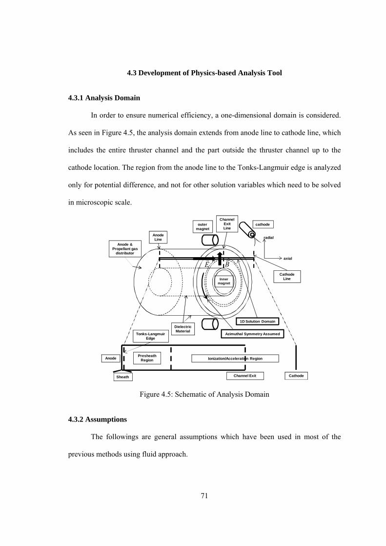
71
4.3 Development of Physics-based Analysis Tool
4.3.1 Analysis Domain
In order to ensure numerical efficiency, a one-dimensional domain is considered.
As seen in Figure 4.5, the analysis domain extends from anode line to cathode line, which
includes the entire thruster channel and the part outside the thruster channel up to the
cathode location. The region from the anode line to the Tonks-Langmuir edge is analyzed
only for potential difference, and not for other solution variables which need to be solved
in microscopic scale.
E
B
Anode &Propellant gas
distributor
cathode
Innermagnet
outermagnet
axial
radial
DielectricMaterial
AnodeLine
Cathode Line
1D Solution Domain
ChannelExitLine
Azimuthal Symmetry Assumed
Anode
CathodeChannel Exit
Presheath Region
Sheath
Ionization/Acceleration Region
Tonks-LangmuirEdge
Figure 4.5: Schematic of Analysis Domain
4.3.2 Assumptions
The followings are general assumptions which have been used in most of the
previous methods using fluid approach.
72
1)Cylindrical coordinates are used: ),,( zr
2)Steady state solution is sought: 0t
3)Azimuthal symmetry is assumed and radial variations are neglected:
0
r
4)Quasi-neutrality is assumed: ei nn
5)All mean velocities in r and are neglected except for electron mean velocity
in the direction.
6)Neutral and ion temperatures are neglected: ein TTT ,0
7)Electron inertia terms are neglected: ine mmm 0
8)Neutral velocity is constant throughout the domain and calculated from
assumed anode temperature: KTanode 1000
9)Stress tensor is reduced to pure pressure: eeee kTnpP ~
10)Only axial direction electric field and radial direction magnetic field are
considered: rz eBBeEE
,
11)The velocity distribution function of electrons is Maxwellian.
12)Neutrals and ions are assumed to be collisionless.
13)The excited neutrals by electron excitation collisions are assumed to
immediately give off the excited energy.
The following are the assumptions which are used for developing the current tool
based on these ideas.
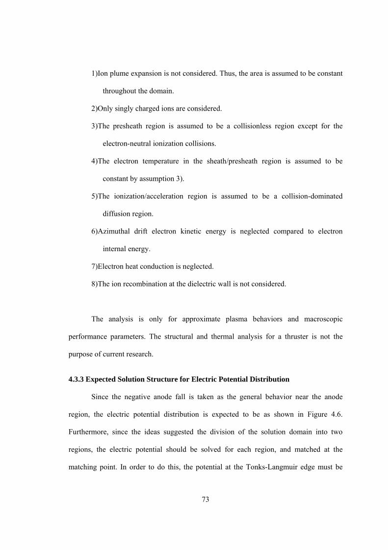
73
1)Ion plume expansion is not considered. Thus, the area is assumed to be constant
throughout the domain.
2)Only singly charged ions are considered.
3)The presheath region is assumed to be a collisionless region except for the
electron-neutral ionization collisions.
4)The electron temperature in the sheath/presheath region is assumed to be
constant by assumption 3).
5)The ionization/acceleration region is assumed to be a collision-dominated
diffusion region.
6)Azimuthal drift electron kinetic energy is neglected compared to electron
internal energy.
7)Electron heat conduction is neglected.
8)The ion recombination at the dielectric wall is not considered.
The analysis is only for approximate plasma behaviors and macroscopic
performance parameters. The structural and thermal analysis for a thruster is not the
purpose of current research.
4.3.3 Expected Solution Structure for Electric Potential Distribution
Since the negative anode fall is taken as the general behavior near the anode
region, the electric potential distribution is expected to be as shown in Figure 4.6.
Furthermore, since the ideas suggested the division of the solution domain into two
regions, the electric potential should be solved for each region, and matched at the
matching point. In order to do this, the potential at the Tonks-Langmuir edge must be
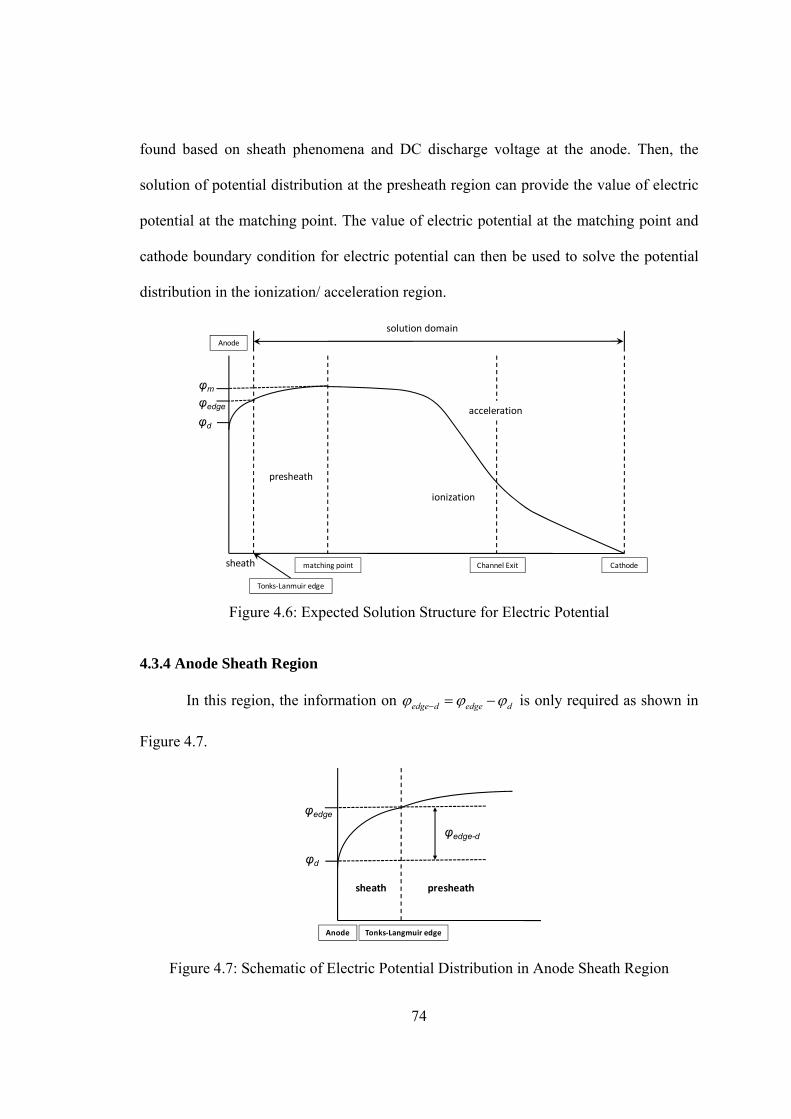
74
found based on sheath phenomena and DC discharge voltage at the anode. Then, the
solution of potential distribution at the presheath region can provide the value of electric
potential at the matching point. The value of electric potential at the matching point and
cathode boundary condition for electric potential can then be used to solve the potential
distribution in the ionization/ acceleration region.
φd
φedge
φm
sheath
presheath
acceleration
ionization
solution domain
Anode
CathodeChannel Exitmatching point
Tonks‐Lanmuir edge
Figure 4.6: Expected Solution Structure for Electric Potential
4.3.4 Anode Sheath Region
In this region, the information on dedgededge is only required as shown in
Figure 4.7.
φd
φedge
sheath presheath
Anode Tonks‐Langmuir edge
φedge-d
Figure 4.7: Schematic of Electric Potential Distribution in Anode Sheath Region
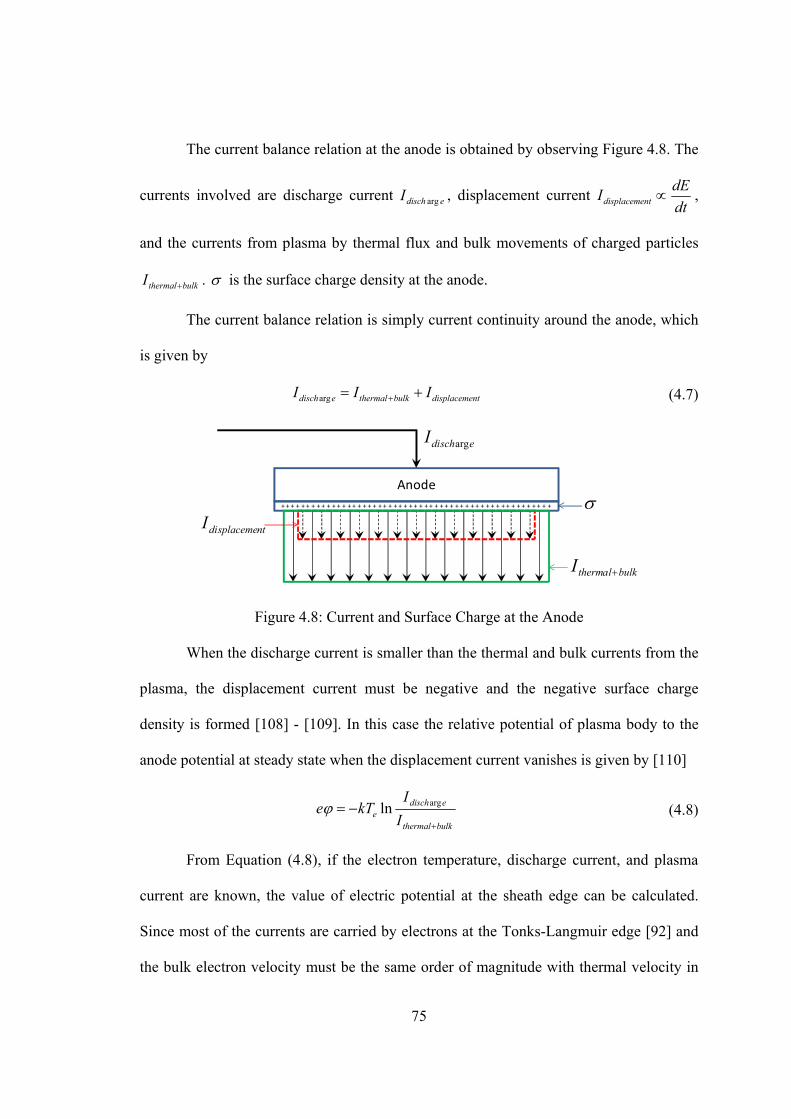
75
The current balance relation at the anode is obtained by observing Figure 4.8. The
currents involved are discharge current edischI arg , displacement current displacement
dEI
dt ,
and the currents from plasma by thermal flux and bulk movements of charged particles
bulkthermalI . is the surface charge density at the anode.
The current balance relation is simply current continuity around the anode, which
is given by
argdisch e thermal bulk displacementI I I (4.7)
Anode
+ + + + + + + + + + + + + + + + + + + + + + + + + + + + + + + + + + + + + + + + + + + + + + + + + + + + +
edischI arg
ntdisplacemeI
bulkthermalI
Figure 4.8: Current and Surface Charge at the Anode
When the discharge current is smaller than the thermal and bulk currents from the
plasma, the displacement current must be negative and the negative surface charge
density is formed [108] - [109]. In this case the relative potential of plasma body to the
anode potential at steady state when the displacement current vanishes is given by [110]
bulkthermal
edische I
IkTe
argln (4.8)
From Equation (4.8), if the electron temperature, discharge current, and plasma
current are known, the value of electric potential at the sheath edge can be calculated.
Since most of the currents are carried by electrons at the Tonks-Langmuir edge [92] and
the bulk electron velocity must be the same order of magnitude with thermal velocity in
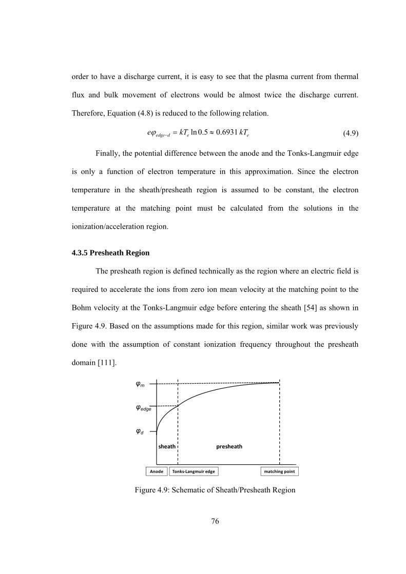
76
order to have a discharge current, it is easy to see that the plasma current from thermal
flux and bulk movement of electrons would be almost twice the discharge current.
Therefore, Equation (4.8) is reduced to the following relation.
eededge kTkTe 6931.05.0ln (4.9)
Finally, the potential difference between the anode and the Tonks-Langmuir edge
is only a function of electron temperature in this approximation. Since the electron
temperature in the sheath/presheath region is assumed to be constant, the electron
temperature at the matching point must be calculated from the solutions in the
ionization/acceleration region.
4.3.5 Presheath Region
The presheath region is defined technically as the region where an electric field is
required to accelerate the ions from zero ion mean velocity at the matching point to the
Bohm velocity at the Tonks-Langmuir edge before entering the sheath [54] as shown in
Figure 4.9. Based on the assumptions made for this region, similar work was previously
done with the assumption of constant ionization frequency throughout the presheath
domain [111].
φd
φedge
sheath presheath
Anode Tonks‐Langmuir edge matching point
φm
Figure 4.9: Schematic of Sheath/Presheath Region
77
In order to apply previous work, the assumption of constant ionization frequency
is also applied for the current case. What is meant here is that the average ionization
frequency in the presheath region may be used to appreciate the previous work. The
questions are how this assumption is reasonable and how to calculate the average
ionization frequency. The first question can be easily justified noting that the ionization
frequency is given by )( eineini TRRnvn , where i is the ionization frequency, nn
is the neutral number density, and )( eiei TRRv is the ionization reaction rate which is
only a function of electron temperature. Since the constant electron temperature in
presheath region is already assumed and the neutral number density is almost constant in
the region near the anode, it is expected that the ionization frequency has little variation
in the presheath region. To be more accurate, the neutral number density variation may be
obtained from presheath solutions such as the ion mean velocity and plasma number
density by using neutral and ion continuity equations.
The governing equations based on assumptions in section 4.3.2 are as follows.
UContinuity equations for neutral, ion, and electron
Sdz
d n
Sdz
d i
Sdz
d e
(4.10)
where, ein ,, represent neutral, ion and electron respectively, nu is the species
number flux, and S is ionization source term, which is given by eine vnnS . The
ionization reaction term, eii vRR , can be calculated as a function of electron energy.
Unlike expressions used in most methods using a fluid approach which are the Arrhenius
law-like form, the regression equation is generated by numerical integration of
experimental data for the ionization cross sections at given electron temperatures with the
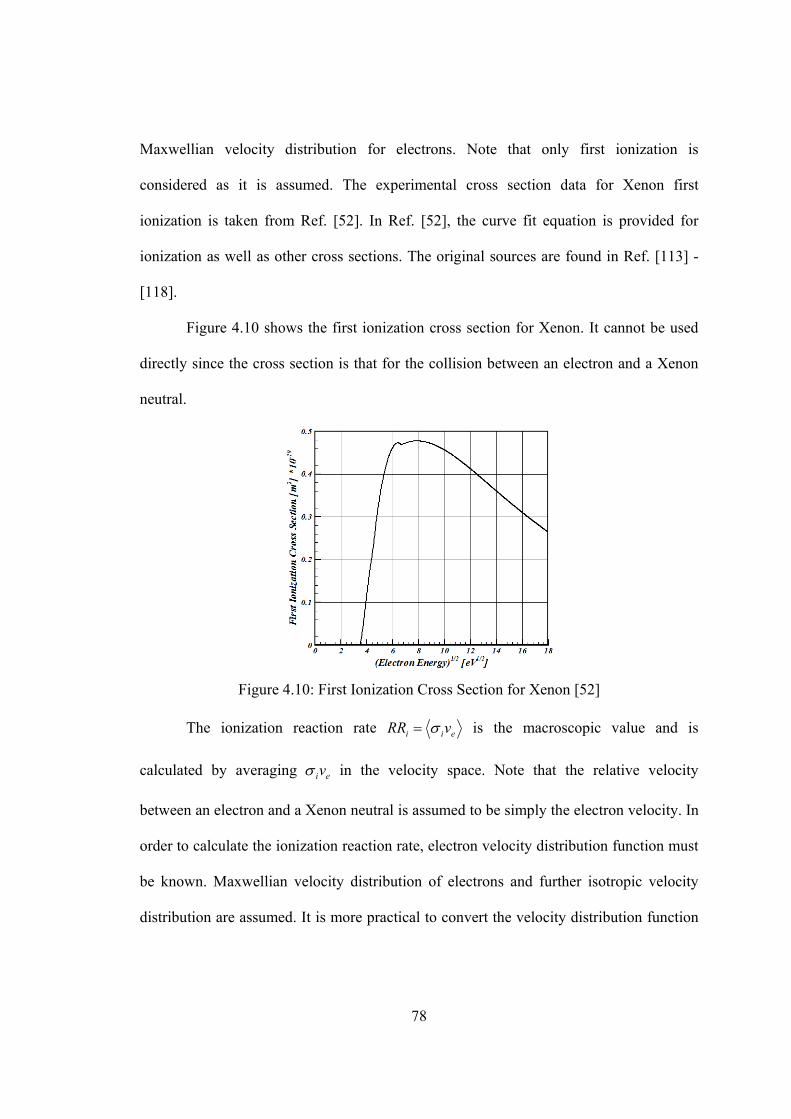
78
Maxwellian velocity distribution for electrons. Note that only first ionization is
considered as it is assumed. The experimental cross section data for Xenon first
ionization is taken from Ref. [52]. In Ref. [52], the curve fit equation is provided for
ionization as well as other cross sections. The original sources are found in Ref. [113] -
[118].
Figure 4.10 shows the first ionization cross section for Xenon. It cannot be used
directly since the cross section is that for the collision between an electron and a Xenon
neutral.
Figure 4.10: First Ionization Cross Section for Xenon [52]
The ionization reaction rate eii vRR is the macroscopic value and is
calculated by averaging eiv in the velocity space. Note that the relative velocity
between an electron and a Xenon neutral is assumed to be simply the electron velocity. In
order to calculate the ionization reaction rate, electron velocity distribution function must
be known. Maxwellian velocity distribution of electrons and further isotropic velocity
distribution are assumed. It is more practical to convert the velocity distribution function
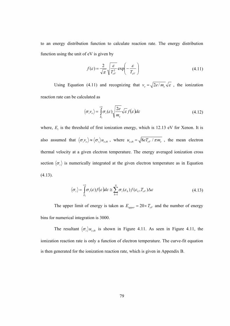
79
to an energy distribution function to calculate reaction rate. The energy distribution
function using the unit of eV is given by
eVeV TTf
exp2
)(3
(4.11)
Using Equation (4.11) and recognizing that ee mev /2 , the ionization
reaction rate can be calculated as
dfm
ev
eE
iei
2)(
1
(4.12)
where, 1E is the threshold of first ionization energy, which is 12.13 eV for Xenon. It is
also assumed that ,i e i e thv u , where , 8 /e th eV eu eT m , the mean electron
thermal velocity at a given electron temperature. The energy averaged ionization cross
section i is numerically integrated at the given electron temperature as in Equation
(4.13).
N
keVkki
E
ii Tfdf1
),()()(1
(4.13)
The upper limit of energy is taken as eVupper TE 20 and the number of energy
bins for numerical integration is 3000.
The resultant ,i e thu is shown in Figure 4.11. As seen in Figure 4.11, the
ionization reaction rate is only a function of electron temperature. The curve-fit equation
is then generated for the ionization reaction rate, which is given in Appendix B.
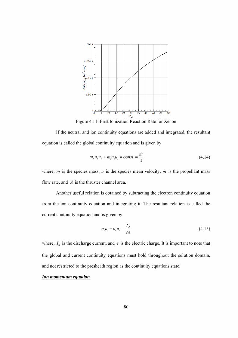
80
Figure 4.11: First Ionization Reaction Rate for Xenon
If the neutral and ion continuity equations are added and integrated, the resultant
equation is called the global continuity equation and is given by
A
mconstunmunm ieinnn
. (4.14)
where, m is the species mass, u is the species mean velocity, m is the propellant mass
flow rate, and A is the thruster channel area.
Another useful relation is obtained by subtracting the electron continuity equation
from the ion continuity equation and integrating it. The resultant relation is called the
current continuity equation and is given by
eA
Iunun d
eeie (4.15)
where, dI is the discharge current, and e is the electric charge. It is important to note that
the global and current continuity equations must hold throughout the solution domain,
and not restricted to the presheath region as the continuity equations state.
UIon momentum equation
81
dz
d
m
en
dz
und
i
eie
)( 2
(4.16)
where, is the electric potential. It is assumed in Equation (4.16) that ions are generated
at zero velocity unlike the ionization/acceleration region where the ions are generated at
neutral velocity. This can be indirectly justified from the experimental results on neutral
velocity, where neutral velocity increases from almost 0 near the anode to some value at
the exit [71]. However, when the global continuity is applied for the presheath, the
constant neutral velocity is used to calculate neutral number density. This is necessary
and reasonable by the fact that first if neutral velocity is zero in the presheath, another
relation is required to obtain neutral number density and second, since neutral velocity is
relatively small compared to ion and electron velocities, the errors from approach above
are expected to be very small.
UElectron momentum equation
dz
den
dz
dnkTor
dz
denkTn
dz
de
eeeee
0)(0 (4.17)
From the assumption of collisionless diffusion in the presheath region, the
collision term in electron momentum equation is neglected. Furthermore, since the
electron temperature is assumed to be constant, the resultant electron momentum
equation has the form of second equation in Equation (4.17).
Equation (4.17) can be easily integrated for plasma number density, which is
given by
)/()0( ekTeee enn (4.18)
If )0(en is the plasma number density at the matching point, ,e mn , the plasma
number density may be obtained for the whole presheath region once the electric
82
potential distribution is found. Equation (4.18) is sometimes called the barometric law. It
simply implies the balance between electrostatic force and pressure force. It is valid for
electrons motion along the magnetic field line and is quite a good approximation across
magnetic fields when the magnetic fields are weak.
The neutral momentum equation is not required since neutral mean velocity is
assumed to be constant. The energy equations for each species are also not required based
on the assumptions in section 4.3.2.
The 6 original unknowns are neutral number density, plasma number density, ion
velocity, electron velocity, electron temperature, and electric potential. Since electron
temperature is assumed to be constant, now 5 unknowns need to be determined, which is
the same as the number of governing equations. Following Kino and Shaw’s work [111],
the ion velocity and electric potential can be simultaneously obtained using the ion
continuity and the ion momentum equations. Then, the plasma number density can be
found using Equation (4.18). The neutral number density can be found using global
continuity. Finally, the electron velocity can be found using current continuity.
The ion continuity and momentum equations are rewritten below.
, ,
( )e ie i ave e n ave i e
d n un n n v
dz
dz
d
m
en
dz
und
i
eie
)( 2
The above equations are non-dimensionalized using the following non-
dimensional variables.
1/2
, 2i
i avee
ms z
kT
i
e
ii u
kT
mv
2/1
2
ekT
e
Then the non-dimensionalized governing equations read
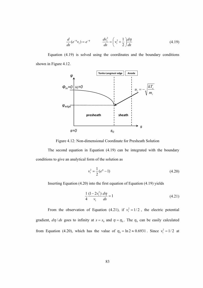
83
eveds
d)( 1
ds
dv
ds
dv
2
121
21 (4.19)
Equation (4.19) is solved using the coordinates and the boundary conditions
shown in Figure 4.12.
Φm=0
φedge
sheathpresheath
AnodeTonks‐Langmuir edge
ui=0
i
ei m
kTu
s=0 s0
φ
s
Figure 4.12: Non-dimensional Coordinate for Presheath Solution
The second equation in Equation (4.19) can be integrated with the boundary
conditions to give an analytical form of the solution as
)1(2
121 ev (4.20)
Inserting Equation (4.20) into the first equation of Equation (4.19) yields
1)21(
4
1
1
21
ds
d
v
v (4.21)
From the observation of Equation (4.21), if 2/121 v , the electric potential
gradient, dsd / goes to infinity at 0ss and 0 . The 0 can be easily calculated
from Equation (4.20), which has the value of 6931.02ln0 . Since 2/121 v at

84
0ss , the Bohm criterion at the Tonks-Langmuir edge is automatically satisfied, which
is iei mkTu / .
Equation (4.21) has an analytical solution with dsd / substituted using Equation
(4.20), which is given by
)2(tan2 11
1 vvs (4.22)
The step by step solution procedure is as follows.
1)Assume plasma number density ,e mn and electron temperature ,e mT at the
matching point.
2)Generate a grid for from 0 to 0 .
3)Calculate 1v using Equation (4.20).
4)Calculate s using Equation (4.22).
5)Calculate average ionization collision frequency, ,i ave
a.Calculate plasma number density using and Equation (4.18).
b.Calculate neutral number density using the global continuity equation.
c.Take the average of neutral number density in the presheath domain.
d.Calculate , , ( )i ave n ave i en RR T
6)Recover dimensional solutions
7)Calculate neutral number density using the global continuity equation again.
8)Calculate electron mean velocity using the current continuity equation.
From the solution procedure, the presheath length is varied depending on the
neutral number density and electron temperature at the matching point as shown in
85
Equation (4.23). The dependence on neutral number density is weak. However, the
electron temperature at the matching point has significant effects on the presheath length.
1/2
0
,
2 epresheath
i i ave
kT sL
m
(4.23)
If the electron temperature at the matching point increases, the average ionization
collision frequency also increases. Although the term 2/1)/2( ie mkT also increases, the
effect of increasing the average ionization collision frequency is greater and this results in
a decrease of the presheath length.
By the sheath and presheath solutions, the value of the electric potential at the
matching point can be determined, which is higher than the discharge voltage at the
anode.
4.3.6 Ionization/Acceleration Region
In this region, 6 unknowns must be determined; neutral number density, plasma
number density, ion mean velocity, electron velocity, electron temperature, and electric
potential. The governing equations based on assumptions in section 4.3.2 are as follows.
UContinuity equations for neutral, ion, and electron
Continuity equations are identical to those for the presheath region as well as
global and current continuities. The integration is performed only for neutral continuity
equation to obtain the neutral number density.
einen
nnn vnn
dz
dnuorS
dz
und )(
(4.24)
Equation (4.24) can be integrated with the boundary condition of neutral number
density at the matching point. Since the ion velocity is 0 there, the neutral number density
86
can be directly calculated from the propellant mass flow rate. Consequently, the neutral
number density in the left region of the matching point is higher than that from the
actually given propellant mass flow rate. This accounts for the ion recombination back to
neutrals at the anode due to ion backflow.
UIon flux-tube or freefall equation
0 0
0 0
1/2 1/20 2 2
0
( ') '( )
2 ( ( ') ( )) 2 ( ( ))
ze i
e
n ni i
n uS z dzn z
e eu z z u z
m m
(4.25)
where, the lower integration limit, 0, represents the matching point, 0nu is the neutral
mean velocity which is constant, and 0i
u is the ion mean velocity at the matching point
which is equal to neutral mean velocity. The ion momentum equation is not used to
enhance numerical robustness. If it is used, the resultant ordinary differential equation
should be solved, which can cause negative plasma number density in the course of
integration. The ion flux-tube equation or ion freefall equation simply uses the ion energy
relationship and ion continuity with a collisionless assumption. What this means is that
ions once created gain energy directly from the electric field and must satisfy the
continuity between two points. Equation (4.25) cannot be used for the case stated in
Equation (4.26), i.e., the electric potential should continue decreasing from the matching
point to the cathode.
0 0
2 202 ( ( ') ( )) 2 ( ( ))n n
i i
e ez z u and z u
m m (4.26)
The second term in Equation (4.25) accounts for the initial ion flux at the
matching point [112]. Although the ion mean velocity is zero at the matching point, here
the ion mean velocity should have the value of the neutral mean velocity which is a
87
phenomenological result from numerical experimentations. If it were not included, the
plasma number density adjacent to the matching point would have a significantly low
value and show discontinuity. The reason why it should be included can also be
explained from the ion momentum equation shown in Equation (4.2), where the ion mean
velocity must be the neutral mean velocity at the matching point in order to have a
regular singular point.
Equation (4.25) is an integral equation with the given information in the context
of a fixed point iteration as explained in section 4.2.4. The integration is performed using
4 point Gauss-Legendre quadrature rule to obtain sufficient accuracy [90].
UElectron momentum equation
,,
( )0 e e m
e e e m e ee
md d een m or
dz dz n
(4.27)
To integrate Equation (4.27), Boeuf’s method is taken [84] - [85]. Since the two
boundary conditions are provided; one at the matching point from the sheath/presheath
solutions, and the other at the cathode, which is assumed to be zero potential. Two
dependent variables can be determined and the electron flux may be expressed as
)()()()( czcz nnee (4.28)
where, c represents the cathode position. Equation (4.28) is obtained using global and
current continuity equations. In this formulation, since neutral flux distribution is
calculated from the integration of Equation (4.24), the unknown is )(ce . Since )(ce
can be considered as a parameter in the ODE to be determined, )(ce can be calculated
from the general way of implementing an additional ODE, which should be solved with
two boundary conditions.
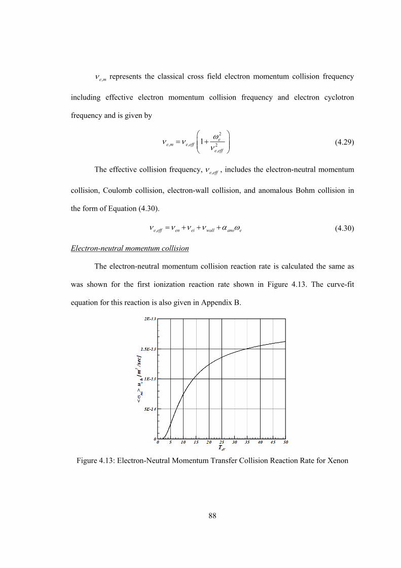
88
,e m represents the classical cross field electron momentum collision frequency
including effective electron momentum collision frequency and electron cyclotron
frequency and is given by
2
, , 2,
1 ee m e eff
e eff
(4.29)
The effective collision frequency, ,e eff , includes the electron-neutral momentum
collision, Coulomb collision, electron-wall collision, and anomalous Bohm collision in
the form of Equation (4.30).
,e eff en ei wall ano e (4.30)
UElectron-neutral momentum collision
The electron-neutral momentum collision reaction rate is calculated the same as
was shown for the first ionization reaction rate shown in Figure 4.13. The curve-fit
equation for this reaction is also given in Appendix B.
Figure 4.13: Electron-Neutral Momentum Transfer Collision Reaction Rate for Xenon
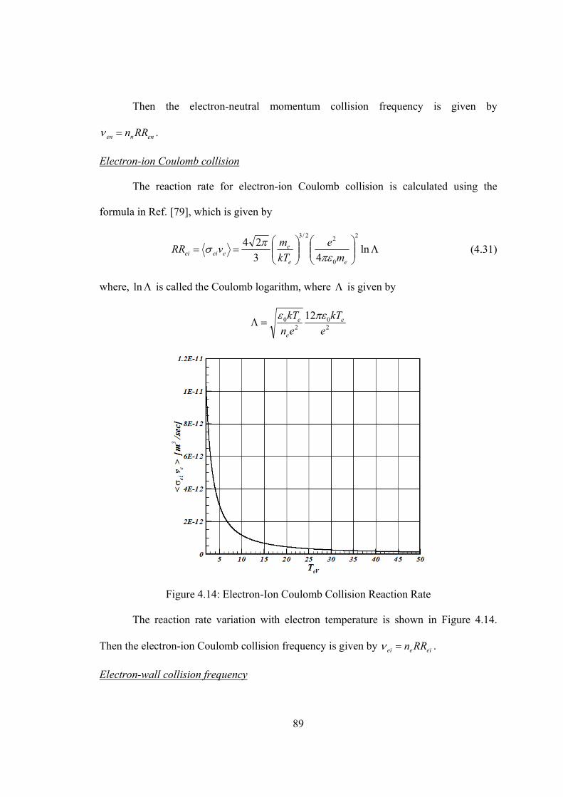
89
Then the electron-neutral momentum collision frequency is given by
ennen RRn .
UElectron-ion Coulomb collision
The reaction rate for electron-ion Coulomb collision is calculated using the
formula in Ref. [79], which is given by
ln
43
242
0
22/3
ee
eeeiei m
e
kT
mvRR
(4.31)
where, ln is called the Coulomb logarithm, where is given by
20
20 12
e
kT
en
kT e
e
e
Figure 4.14: Electron-Ion Coulomb Collision Reaction Rate
The reaction rate variation with electron temperature is shown in Figure 4.14.
Then the electron-ion Coulomb collision frequency is given by eieei RRn .
UElectron-wall collision frequency
90
The model of electron-wall collision is taken from Ref. [78]. Ref. [78] analyzed
the electron continuity and radial momentum equations and proposed the wall
recombination frequency as
i
e
c
ww m
kT
h
~
(4.32)
where, w is the wall recombination frequency, ch is the channel width, and w~ is
governed by the radial presheath plasma dynamics with a value between 0.7 and 1.2 for
typical discharge conditions. Here, the value of 1 is taken. Then the electron-wall
collision frequency is given by
w
wmwmwall where
1
, (4.33)
where, w is the effective SEE yield, which is approximated by
**
*1
,
,/)(
eew
eeeew
TT
TTTTT
(4.34)
where, 983.0* w , 1* 968.0 TTe , and 11 66.0~ ET . 1E is the energy of electron which
yields 100% of SEE and its value is 50eV for a Boron Nitride wall material. Equation
(4.34) indicates that the effective SEE is limited to *w at an electron temperature over
*ee TT . This means that the electron-repelling sheath at the wall prevents further
electron flux to the wall at a higher electron temperature, which is called the Charge
Saturation Regime (CSR).
UAnomalous Bohm collision frequency
As explained in section 4.2.4, this topic is still not in consensus among HET
researchers. Thus, the most recent experimental results are taken to implement it for
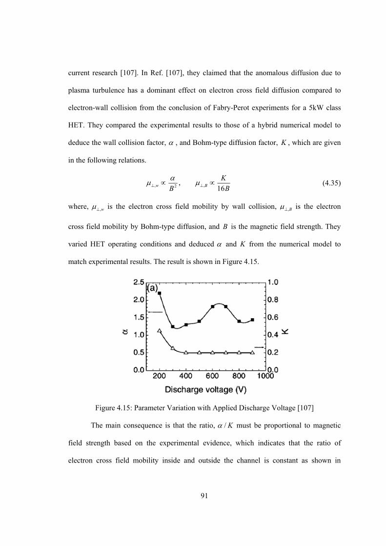
91
current research [107]. In Ref. [107], they claimed that the anomalous diffusion due to
plasma turbulence has a dominant effect on electron cross field diffusion compared to
electron-wall collision from the conclusion of Fabry-Perot experiments for a 5kW class
HET. They compared the experimental results to those of a hybrid numerical model to
deduce the wall collision factor, , and Bohm-type diffusion factor, K , which are given
in the following relations.
B
K
B Bw 16, ,2, (4.35)
where, w, is the electron cross field mobility by wall collision, B, is the electron
cross field mobility by Bohm-type diffusion, and B is the magnetic field strength. They
varied HET operating conditions and deduced and K from the numerical model to
match experimental results. The result is shown in Figure 4.15.
Figure 4.15: Parameter Variation with Applied Discharge Voltage [107]
The main consequence is that the ratio, K/ must be proportional to magnetic
field strength based on the experimental evidence, which indicates that the ratio of
electron cross field mobility inside and outside the channel is constant as shown in
92
Equation (4.36). This led them to conclude that the same mechanism must hold for the
regions inside and outside the channel.
,
,
1.in
out
constK B
(4.36)
They proposed the same form of mobility expressions for inside and outside the
channel and the value of each parameter given by.
, ,, 0.1 0.216 16
in outin in out out
K KK K
B B (4.37)
In order to adapt the results of Figure 4.15 and Equation (4.37) to the current form
of eanoB , the following curve fit equations are proposed to cover large discharge
voltage variations. By letting anoano /1ˆ ,
1)Inside the thruster channel
,minˆ 100 150ano at V ,max
ˆ 160 400ano over V
2,max ,min
,min ,max,min
ˆ ˆ400ˆ ˆ ˆ1 exp , log 1
ˆ400 150ano anod
ano ano anoano
VA where A
2)Outside the thruster channel
The same form as inside the channel but with a different ,min ,maxˆ ˆano anoand .
,minˆ 50 150ano at V ,max
ˆ 80 400ano over V
Furthermore in order to have numerical stability, the smooth variation of ano
between inside and outside the channel is implemented as shown in Equation(4.38).
93
,
, , , ,
,
ˆ
ˆ ˆ ˆ ˆˆ ( ) cos
2 2
ˆ
ano in
ano in ano out ano in ano outano s
ss
ano out
z Lz L
z L z L LL
z L L
(4.38)
where, L is the thruster channel length and sL is the smooth transition distance, which
must be less than the distance between the thruster exit to the cathode line. Here, sL is
taken to be half of the distance between the thruster exit to the cathode line.
UElectron energy equation
,
5( )
3 e e e e e e
de E n
dz ee kT2
3 (4.39)
Equation (4.39) can be integrated with a boundary condition at the cathode line.
The electron temperature at the cathode is usually taken to be 2eV~3eV. Here, 2eV is
taken as a boundary condition. Equation (4.39) can be expanded to give the form for
dzd e / as
,3 3
5 5e ee e i
e ee e
nd neE
dz
(4.40)
The electron energy loss frequency, ,e , consists of several loss mechanisms
such as ionization, excitation, and wall-collision energy loss.
UIonization and excitation energy loss frequency
The energy loss rate by ionization and excitation is given by
excexciionexcione / (4.41)
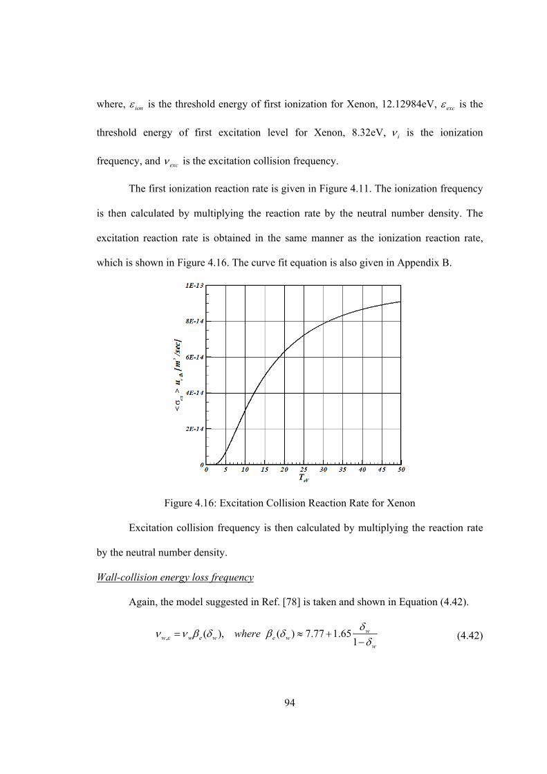
94
where, ion is the threshold energy of first ionization for Xenon, 12.12984eV, exc is the
threshold energy of first excitation level for Xenon, 8.32eV, i is the ionization
frequency, and exc is the excitation collision frequency.
The first ionization reaction rate is given in Figure 4.11. The ionization frequency
is then calculated by multiplying the reaction rate by the neutral number density. The
excitation reaction rate is obtained in the same manner as the ionization reaction rate,
which is shown in Figure 4.16. The curve fit equation is also given in Appendix B.
Figure 4.16: Excitation Collision Reaction Rate for Xenon
Excitation collision frequency is then calculated by multiplying the reaction rate
by the neutral number density.
UWall-collision energy loss frequency
Again, the model suggested in Ref. [78] is taken and shown in Equation (4.42).
, ( ), ( ) 7.77 1.651
ww w e w e w
w
where
(4.42)
95
where, ww and are given in Equation (4.32) and Equation (4.34), respectively.
4.3.7 Matching Two Solutions
In order to match two solutions, all the values of the unknowns from the presheath
and ionization/acceleration regions must be the same at the matching point. Since the
unknowns are neutral number density, ion mean velocity, electron mean velocity,
electron temperature, plasma number density, and electric potential, proper strategies for
these to match must be provided. The strategies are as follows.
1)Neutral number density: Neutral number density is constant and fixed as the one
obtained from the given propellant mass flow rate. This is a consequence of
global continuity since the ion velocity is zero at the matching point. This
value also plays a role of a boundary condition for neutral density integration
in the ionization/acceleration region. Neutral number density distribution in
the presheath is obtained from global continuity.
2)Ion mean velocity: Ion mean velocity is zero at the matching point. This is a
consequence from the assumption of dividing the whole domain into two
regions since the presheath region starts from the edge of main plasma body
where the ion mean velocity is equal to zero. This value also becomes one of
the boundary conditions in the presheath region. Ion mean velocity in the
ionization/acceleration region is obtained from global continuity.
3)Electron mean velocity: Electron mean velocity is obtained from the solution of
ionization/acceleration region by solving the electron momentum equation.
From these solutions, the electron flux at the cathode is obtained and the
electron mean velocity is then calculated using current continuity for the
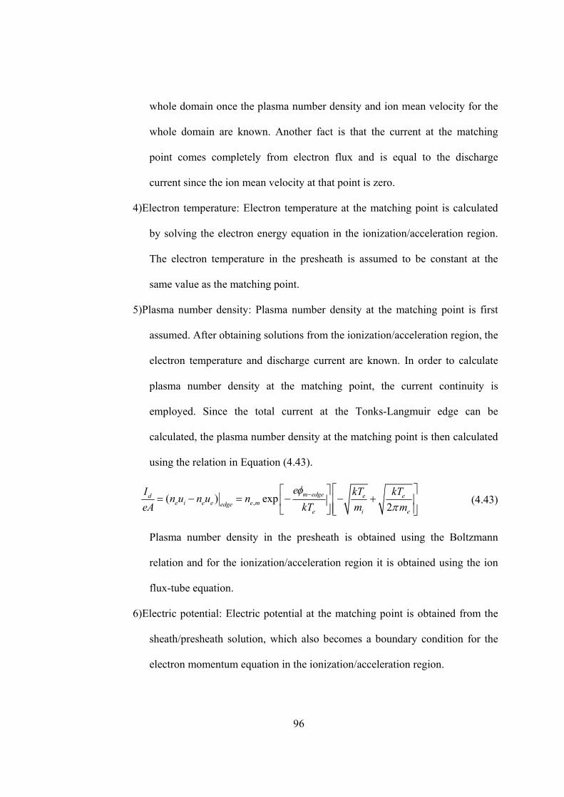
96
whole domain once the plasma number density and ion mean velocity for the
whole domain are known. Another fact is that the current at the matching
point comes completely from electron flux and is equal to the discharge
current since the ion mean velocity at that point is zero.
4)Electron temperature: Electron temperature at the matching point is calculated
by solving the electron energy equation in the ionization/acceleration region.
The electron temperature in the presheath is assumed to be constant at the
same value as the matching point.
5)Plasma number density: Plasma number density at the matching point is first
assumed. After obtaining solutions from the ionization/acceleration region, the
electron temperature and discharge current are known. In order to calculate
plasma number density at the matching point, the current continuity is
employed. Since the total current at the Tonks-Langmuir edge can be
calculated, the plasma number density at the matching point is then calculated
using the relation in Equation (4.43).
,( ) exp2
m edged e ee i e e e medge
e i e
eI kT kTn u n u n
eA kT m m
(4.43)
Plasma number density in the presheath is obtained using the Boltzmann
relation and for the ionization/acceleration region it is obtained using the ion
flux-tube equation.
6)Electric potential: Electric potential at the matching point is obtained from the
sheath/presheath solution, which also becomes a boundary condition for the
electron momentum equation in the ionization/acceleration region.
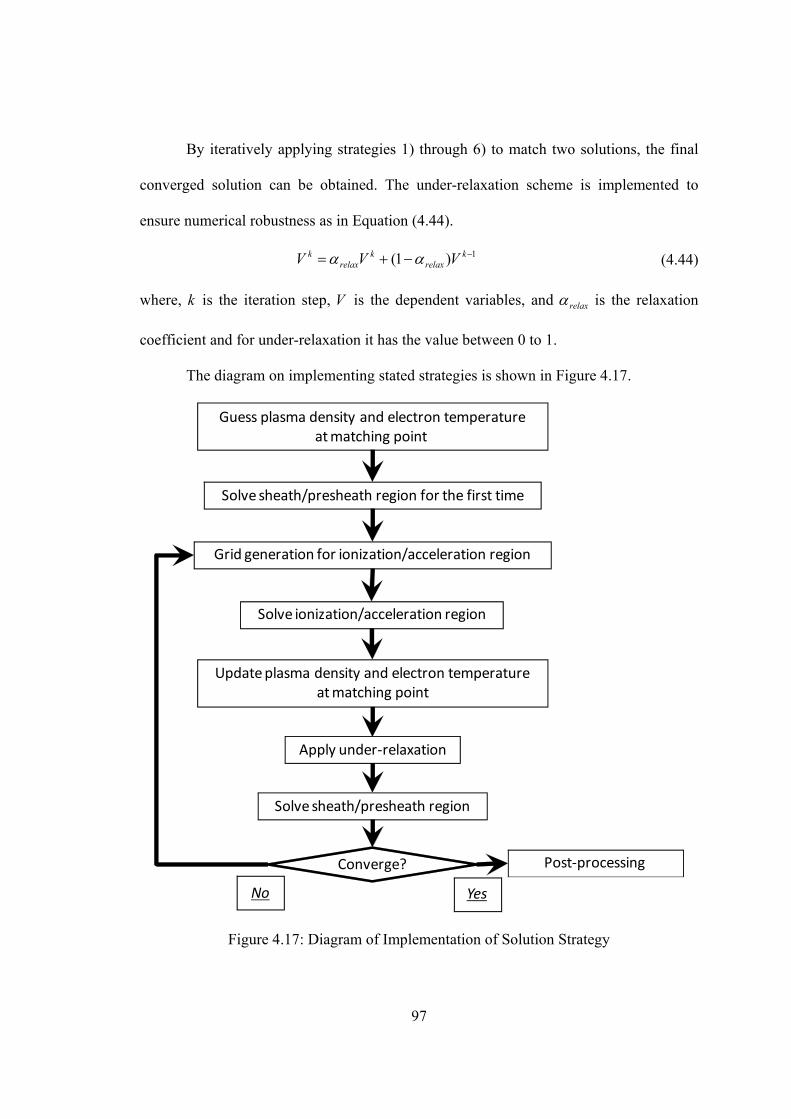
97
By iteratively applying strategies 1) through 6) to match two solutions, the final
converged solution can be obtained. The under-relaxation scheme is implemented to
ensure numerical robustness as in Equation (4.44).
1)1( krelax
krelax
k VVV (4.44)
where, k is the iteration step, V is the dependent variables, and relax is the relaxation
coefficient and for under-relaxation it has the value between 0 to 1.
The diagram on implementing stated strategies is shown in Figure 4.17.
Guess plasma density and electron temperatureat matching point
Solve sheath/presheath region for the first time
Grid generation for ionization/acceleration region
Solve ionization/acceleration region
Update plasma density and electron temperatureat matching point
Solve sheath/presheath region
Apply under‐relaxation
Converge? Post‐processing
YesNo
Figure 4.17: Diagram of Implementation of Solution Strategy

98
4.3.8 Non-Dimensionalization
Before solving the governing equations, they should be properly non-
dimensionalized with appropriate reference values. For the current governing equations,
the orders of magnitude of the variables are quite different. For example, number density
is on the order of 1810 , but electron temperature is on the order of 10 . Furthermore, the
masses of species have considerably low orders of magnitude and the electrical charge
quantity is also very low magnitude. Thus, if they are used with original units, it might
cause serious numerical errors such as round-off and truncation. The machine precision
for calculation must be carefully examined in this regard.
Reference values for proper non-dimensionalizations of each variable are given in
Appendix C. These values have been typically used in most of the previous work.
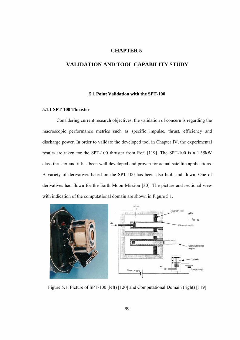
99
CHAPTER 5
VALIDATION AND TOOL CAPABILITY STUDY
5.1 Point Validation with the SPT-100
5.1.1 SPT-100 Thruster
Considering current research objectives, the validation of concern is regarding the
macroscopic performance metrics such as specific impulse, thrust, efficiency and
discharge power. In order to validate the developed tool in Chapter IV, the experimental
results are taken for the SPT-100 thruster from Ref. [119]. The SPT-100 is a 1.35kW
class thruster and it has been well developed and proven for actual satellite applications.
A variety of derivatives based on the SPT-100 has been also built and flown. One of
derivatives had flown for the Earth-Moon Mission [30]. The picture and sectional view
with indication of the computational domain are shown in Figure 5.1.
Figure 5.1: Picture of SPT-100 (left) [120] and Computational Domain (right) [119]
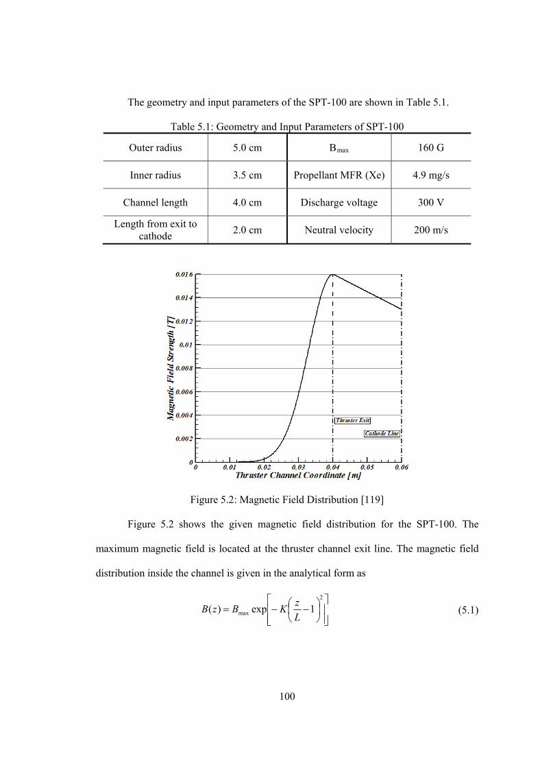
100
The geometry and input parameters of the SPT-100 are shown in Table 5.1.
Table 5.1: Geometry and Input Parameters of SPT-100
Outer radius 5.0 cm BRmax 160 G
Inner radius 3.5 cm Propellant MFR (Xe) 4.9 mg/s
Channel length 4.0 cm Discharge voltage 300 V
Length from exit to cathode
2.0 cm Neutral velocity 200 m/s
Figure 5.2: Magnetic Field Distribution [119]
Figure 5.2 shows the given magnetic field distribution for the SPT-100. The
maximum magnetic field is located at the thruster channel exit line. The magnetic field
distribution inside the channel is given in the analytical form as
2
max 1exp)(L
zKBzB (5.1)
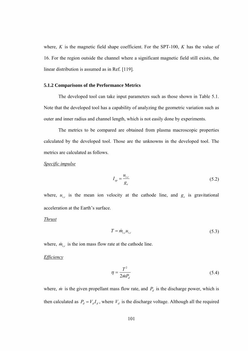
101
where, K is the magnetic field shape coefficient. For the SPT-100, K has the value of
16. For the region outside the channel where a significant magnetic field still exists, the
linear distribution is assumed as in Ref. [119].
5.1.2 Comparisons of the Performance Metrics
The developed tool can take input parameters such as those shown in Table 5.1.
Note that the developed tool has a capability of analyzing the geometric variation such as
outer and inner radius and channel length, which is not easily done by experiments.
The metrics to be compared are obtained from plasma macroscopic properties
calculated by the developed tool. Those are the unknowns in the developed tool. The
metrics are calculated as follows.
USpecific impulse
,i csp
e
uI
g (5.2)
where, ,i cu is the mean ion velocity at the cathode line, and eg is gravitational
acceleration at the Earth’s surface.
UThrust
, ,i c i cT m u (5.3)
where, ,i cm is the ion mass flow rate at the cathode line.
UEfficiency
dPm
T2
2
(5.4)
where, m is the given propellant mass flow rate, and dP is the discharge power, which is
then calculated as ddd IVP , where dV is the discharge voltage. Although all the required
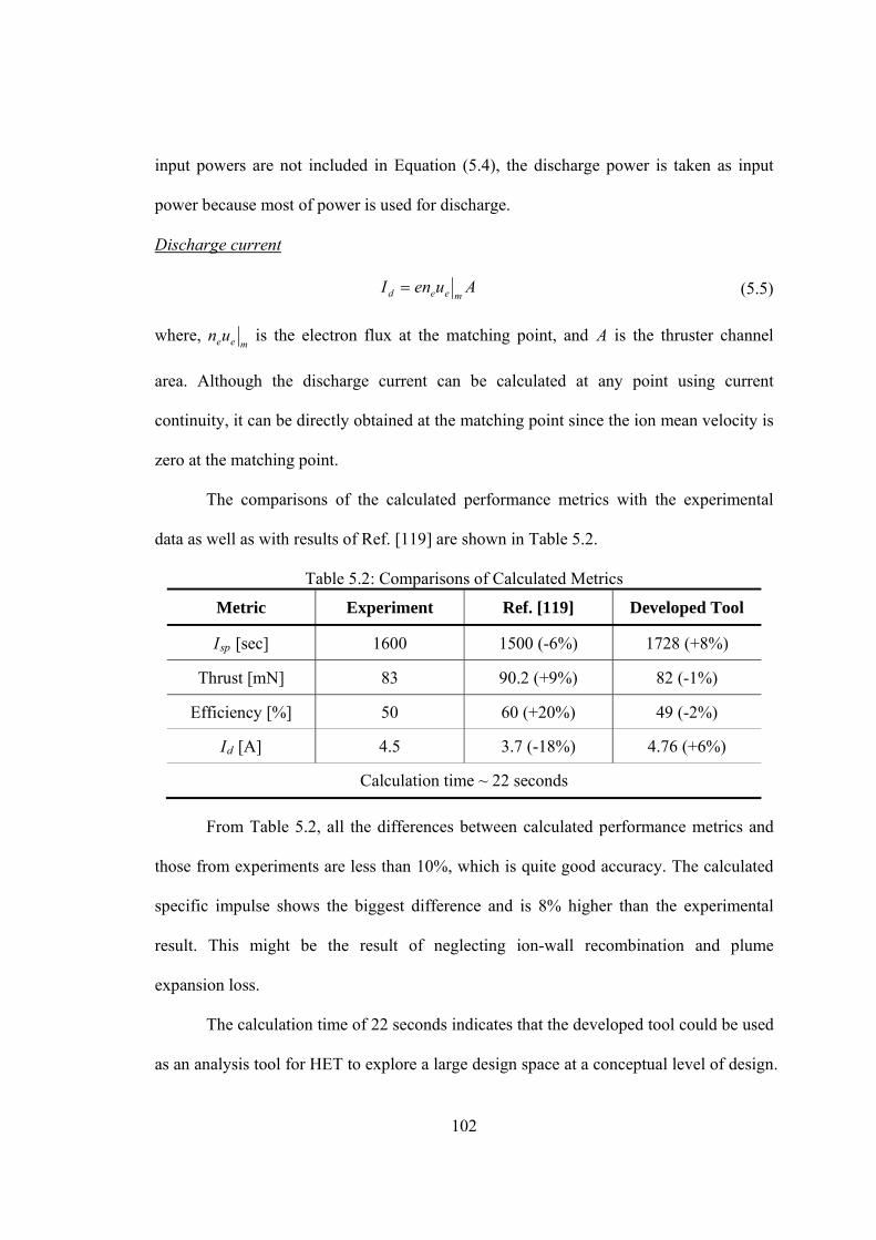
102
input powers are not included in Equation (5.4), the discharge power is taken as input
power because most of power is used for discharge.
UDischarge current
AuenImeed (5.5)
where, meeun is the electron flux at the matching point, and A is the thruster channel
area. Although the discharge current can be calculated at any point using current
continuity, it can be directly obtained at the matching point since the ion mean velocity is
zero at the matching point.
The comparisons of the calculated performance metrics with the experimental
data as well as with results of Ref. [119] are shown in Table 5.2.
Table 5.2: Comparisons of Calculated Metrics
Metric Experiment Ref. [119] Developed Tool
IRspR [sec] 1600 1500 (-6%) 1728 (+8%)
Thrust [mN] 83 90.2 (+9%) 82 (-1%)
Efficiency [%] 50 60 (+20%) 49 (-2%)
IRdR [A] 4.5 3.7 (-18%) 4.76 (+6%)
Calculation time ~ 22 seconds
From Table 5.2, all the differences between calculated performance metrics and
those from experiments are less than 10%, which is quite good accuracy. The calculated
specific impulse shows the biggest difference and is 8% higher than the experimental
result. This might be the result of neglecting ion-wall recombination and plume
expansion loss.
The calculation time of 22 seconds indicates that the developed tool could be used
as an analysis tool for HET to explore a large design space at a conceptual level of design.
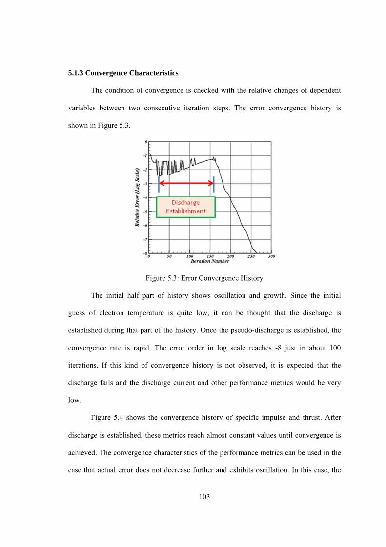
103
5.1.3 Convergence Characteristics
The condition of convergence is checked with the relative changes of dependent
variables between two consecutive iteration steps. The error convergence history is
shown in Figure 5.3.
Figure 5.3: Error Convergence History
The initial half part of history shows oscillation and growth. Since the initial
guess of electron temperature is quite low, it can be thought that the discharge is
established during that part of the history. Once the pseudo-discharge is established, the
convergence rate is rapid. The error order in log scale reaches -8 just in about 100
iterations. If this kind of convergence history is not observed, it is expected that the
discharge fails and the discharge current and other performance metrics would be very
low.
Figure 5.4 shows the convergence history of specific impulse and thrust. After
discharge is established, these metrics reach almost constant values until convergence is
achieved. The convergence characteristics of the performance metrics can be used in the
case that actual error does not decrease further and exhibits oscillation. In this case, the
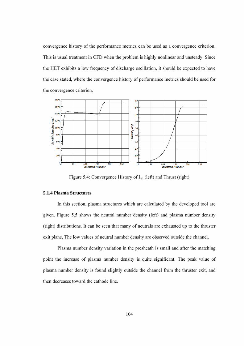
104
convergence history of the performance metrics can be used as a convergence criterion.
This is usual treatment in CFD when the problem is highly nonlinear and unsteady. Since
the HET exhibits a low frequency of discharge oscillation, it should be expected to have
the case stated, where the convergence history of performance metrics should be used for
the convergence criterion.
Figure 5.4: Convergence History of IRspR (left) and Thrust (right)
5.1.4 Plasma Structures
In this section, plasma structures which are calculated by the developed tool are
given. Figure 5.5 shows the neutral number density (left) and plasma number density
(right) distributions. It can be seen that many of neutrals are exhausted up to the thruster
exit plane. The low values of neutral number density are observed outside the channel.
Plasma number density variation in the presheath is small and after the matching
point the increase of plasma number density is quite significant. The peak value of
plasma number density is found slightly outside the channel from the thruster exit, and
then decreases toward the cathode line.
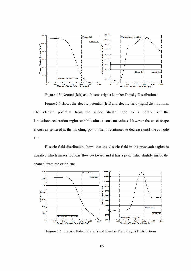
105
Figure 5.5: Neutral (left) and Plasma (right) Number Density Distributions
Figure 5.6 shows the electric potential (left) and electric field (right) distributions.
The electric potential from the anode sheath edge to a portion of the
ionization/acceleration region exhibits almost constant values. However the exact shape
is convex centered at the matching point. Then it continues to decrease until the cathode
line.
Electric field distribution shows that the electric field in the presheath region is
negative which makes the ions flow backward and it has a peak value slightly inside the
channel from the exit plane.
Figure 5.6: Electric Potential (left) and Electric Field (right) Distributions
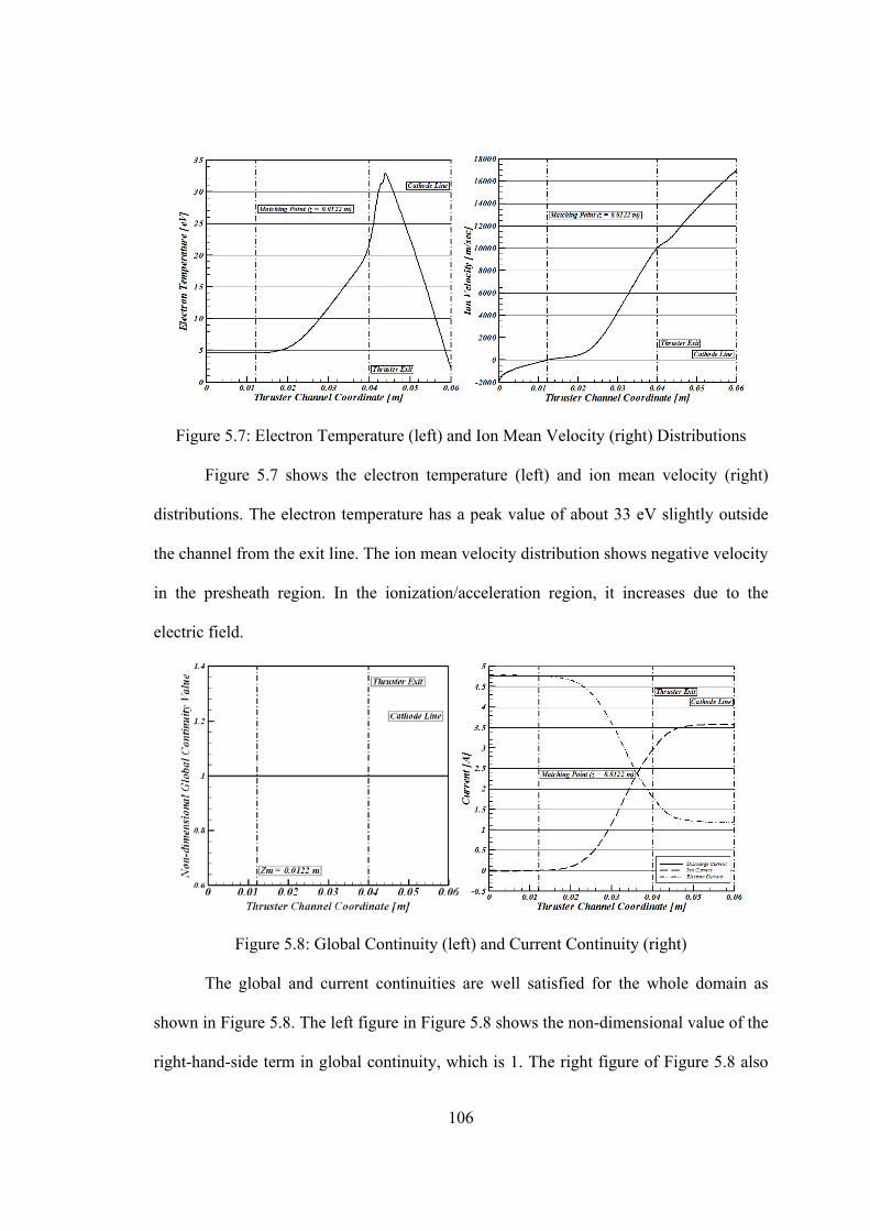
106
Figure 5.7: Electron Temperature (left) and Ion Mean Velocity (right) Distributions
Figure 5.7 shows the electron temperature (left) and ion mean velocity (right)
distributions. The electron temperature has a peak value of about 33 eV slightly outside
the channel from the exit line. The ion mean velocity distribution shows negative velocity
in the presheath region. In the ionization/acceleration region, it increases due to the
electric field.
Figure 5.8: Global Continuity (left) and Current Continuity (right)
The global and current continuities are well satisfied for the whole domain as
shown in Figure 5.8. The left figure in Figure 5.8 shows the non-dimensional value of the
right-hand-side term in global continuity, which is 1. The right figure of Figure 5.8 also
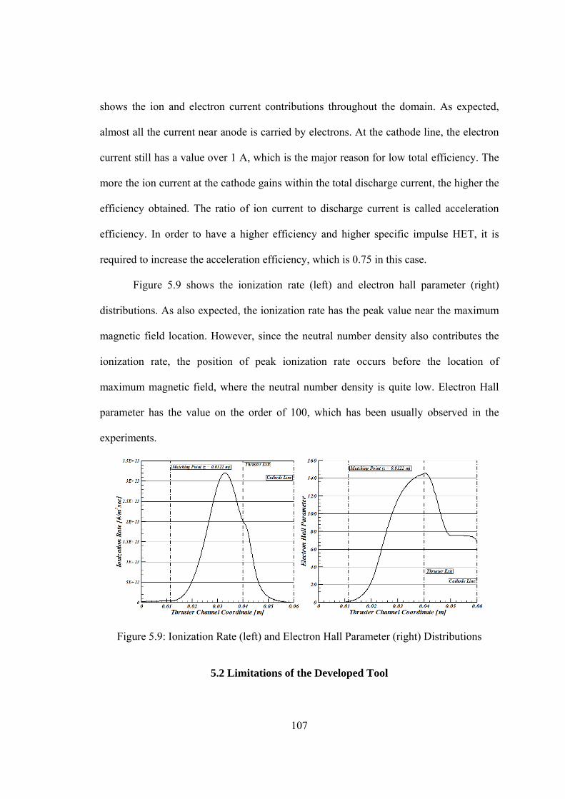
107
shows the ion and electron current contributions throughout the domain. As expected,
almost all the current near anode is carried by electrons. At the cathode line, the electron
current still has a value over 1 A, which is the major reason for low total efficiency. The
more the ion current at the cathode gains within the total discharge current, the higher the
efficiency obtained. The ratio of ion current to discharge current is called acceleration
efficiency. In order to have a higher efficiency and higher specific impulse HET, it is
required to increase the acceleration efficiency, which is 0.75 in this case.
Figure 5.9 shows the ionization rate (left) and electron hall parameter (right)
distributions. As also expected, the ionization rate has the peak value near the maximum
magnetic field location. However, since the neutral number density also contributes the
ionization rate, the position of peak ionization rate occurs before the location of
maximum magnetic field, where the neutral number density is quite low. Electron Hall
parameter has the value on the order of 100, which has been usually observed in the
experiments.
Figure 5.9: Ionization Rate (left) and Electron Hall Parameter (right) Distributions
5.2 Limitations of the Developed Tool
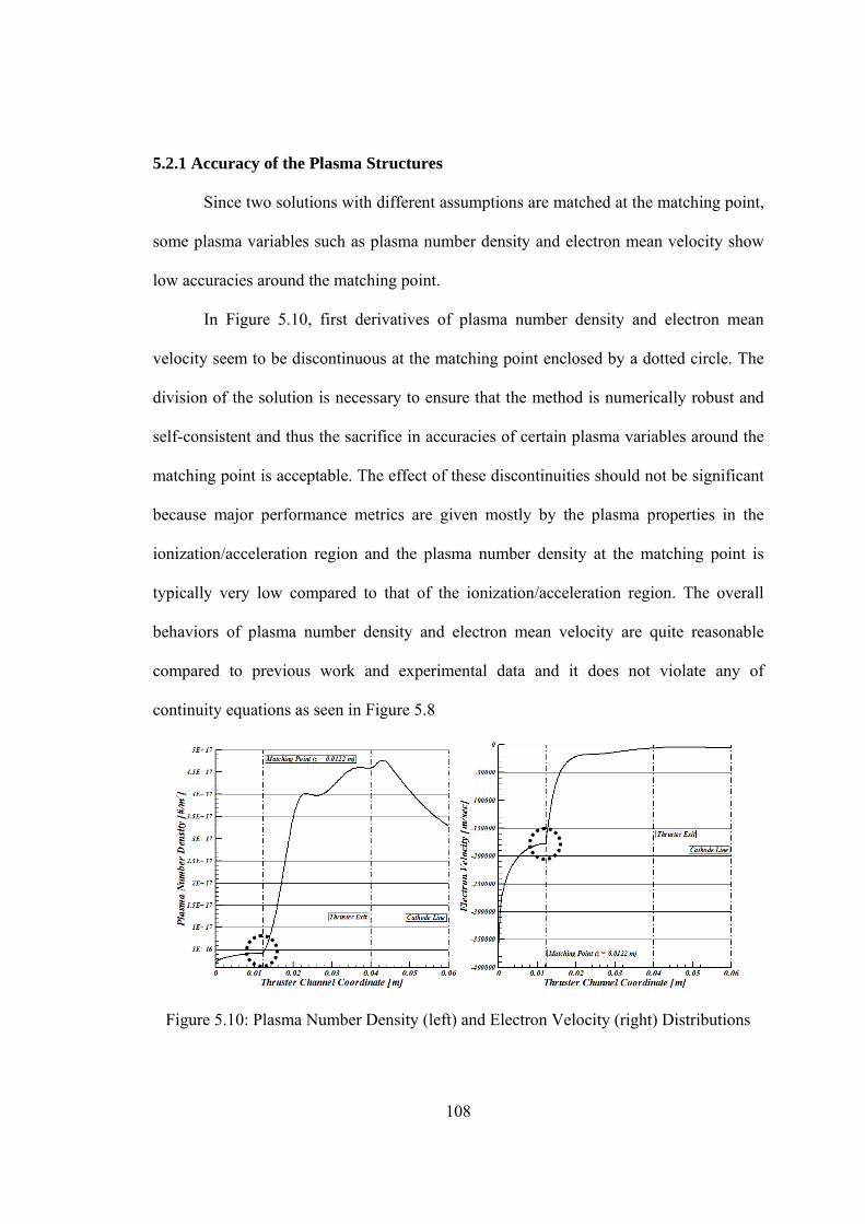
108
5.2.1 Accuracy of the Plasma Structures
Since two solutions with different assumptions are matched at the matching point,
some plasma variables such as plasma number density and electron mean velocity show
low accuracies around the matching point.
In Figure 5.10, first derivatives of plasma number density and electron mean
velocity seem to be discontinuous at the matching point enclosed by a dotted circle. The
division of the solution is necessary to ensure that the method is numerically robust and
self-consistent and thus the sacrifice in accuracies of certain plasma variables around the
matching point is acceptable. The effect of these discontinuities should not be significant
because major performance metrics are given mostly by the plasma properties in the
ionization/acceleration region and the plasma number density at the matching point is
typically very low compared to that of the ionization/acceleration region. The overall
behaviors of plasma number density and electron mean velocity are quite reasonable
compared to previous work and experimental data and it does not violate any of
continuity equations as seen in Figure 5.8
Figure 5.10: Plasma Number Density (left) and Electron Velocity (right) Distributions
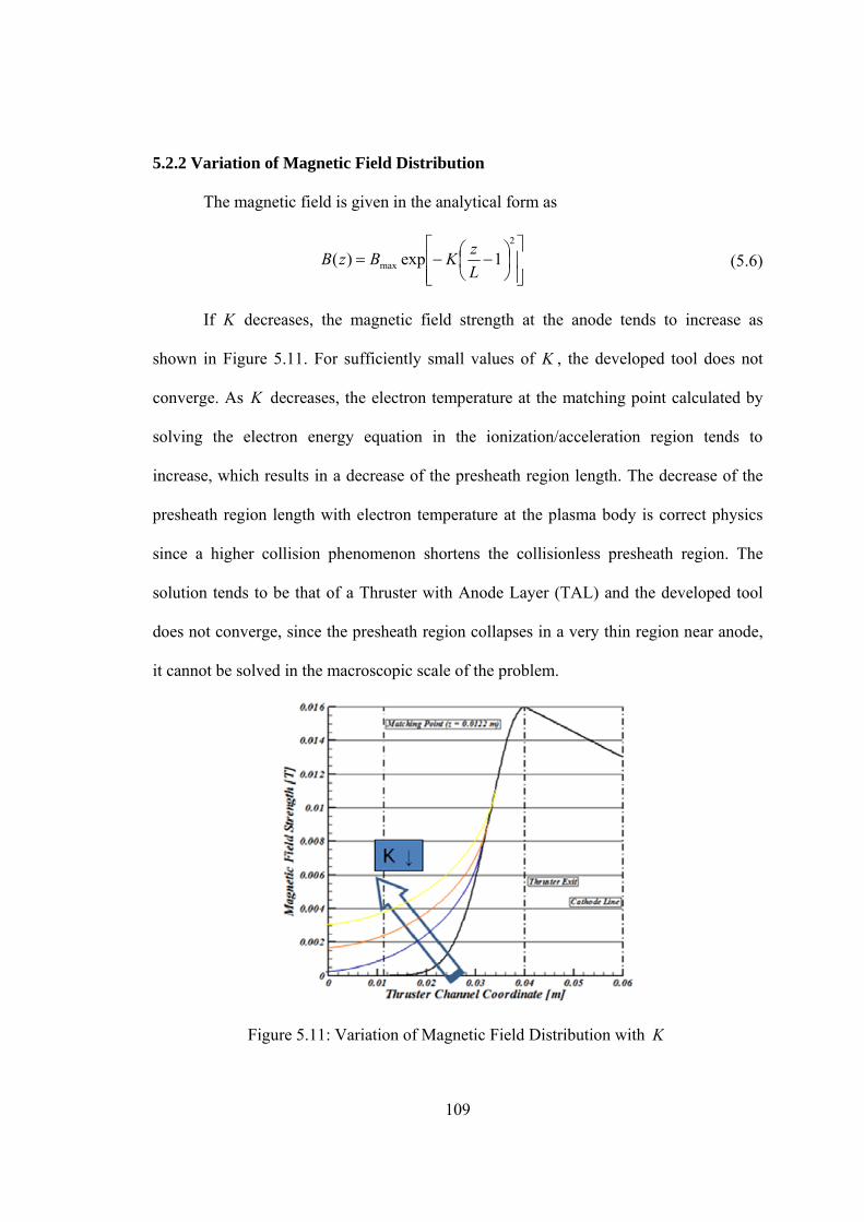
109
5.2.2 Variation of Magnetic Field Distribution
The magnetic field is given in the analytical form as
2
max 1exp)(L
zKBzB (5.6)
If K decreases, the magnetic field strength at the anode tends to increase as
shown in Figure 5.11. For sufficiently small values of K , the developed tool does not
converge. As K decreases, the electron temperature at the matching point calculated by
solving the electron energy equation in the ionization/acceleration region tends to
increase, which results in a decrease of the presheath region length. The decrease of the
presheath region length with electron temperature at the plasma body is correct physics
since a higher collision phenomenon shortens the collisionless presheath region. The
solution tends to be that of a Thruster with Anode Layer (TAL) and the developed tool
does not converge, since the presheath region collapses in a very thin region near anode,
it cannot be solved in the macroscopic scale of the problem.
Figure 5.11: Variation of Magnetic Field Distribution with K
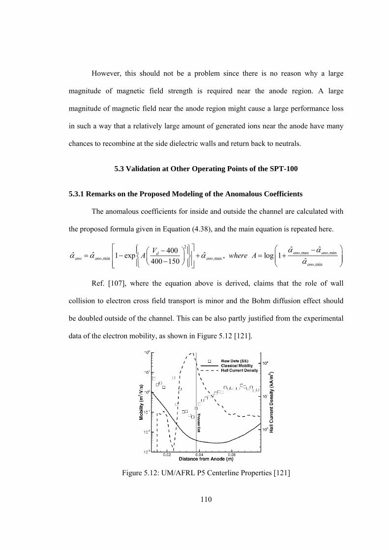
110
However, this should not be a problem since there is no reason why a large
magnitude of magnetic field strength is required near the anode region. A large
magnitude of magnetic field near the anode region might cause a large performance loss
in such a way that a relatively large amount of generated ions near the anode have many
chances to recombine at the side dielectric walls and return back to neutrals.
5.3 Validation at Other Operating Points of the SPT-100
5.3.1 Remarks on the Proposed Modeling of the Anomalous Coefficients
The anomalous coefficients for inside and outside the channel are calculated with
the proposed formula given in Equation (4.38), and the main equation is repeated here.
2,max ,min
,min ,max,min
ˆ ˆ400ˆ ˆ ˆ1 exp , log 1
ˆ400 150ano anod
ano ano anoano
VA where A
Ref. [107], where the equation above is derived, claims that the role of wall
collision to electron cross field transport is minor and the Bohm diffusion effect should
be doubled outside of the channel. This can be also partly justified from the experimental
data of the electron mobility, as shown in Figure 5.12 [121].
Figure 5.12: UM/AFRL P5 Centerline Properties [121]
111
Figure 5.12 shows that the difference between experimental mobility and classical
mobility outside of the channel is far greater than the difference inside. In the current
implementation, the anomalous coefficients are only a function of discharge voltage and
those are fixed as ,ˆ 160ano in and ,
ˆ 80ano out over 400 V. Furthermore, the equation is
derived based on the experimental results only from the comparison with a 5 kW HET. In
order to verify these simple relations, further validation is conducted with the variation of
the anode propellant mass flow rate. The experimental data is taken from Table V of Ref.
[16] since the lowest facility pressure was achieved in that experiment. The specific
impulse and efficiency in the experimental data include the cathode mass flow rate.
Therefore, the calculation of performance metrics should be expanded.
5.3.2 Redefinition of Performance Metrics
More thorough definitions for the performance metrics are given below.
USpecific Impulse
Specific impulse is given in the same form of Equation (5.2). The total specific
impulse incorporates cathode mass flow rate, the form of which will be given later.
UTotal power required
Total power required to sustain the discharge can be expressed as follows.
tot d cath magP P P P (5.7)
where, dP is the discharge power and it is the product of the discharge voltage and
discharge current, cathP is the power required to operate the cathode and it is usually less
than 10% of dP , although it varies with the cathode type used, and magP is the power
112
required to produce magnetic field and it would be zero if permanent magnets were to be
used.
UAnode Efficiency
Anode efficiency is expressed as
2
2anoa d
T
m P
(5.8)
where, ano is the anode efficiency, and am is the anode propellant mass flow rate. The
anode efficiency is a function of propellant utilization, ion beam divergence, ionization
rate, and the amount of ion recombination. Thus, it can be separated into several
efficiency terms characterizing each effect on the resultant anode efficiency. The thrust
can be expanded by
, , , , , ,a i i c i c n c n c i c i cT m u m u m u m u (5.9)
where ,i cm and ,n cm are the ion and neutral mass flow rate at the cathode line,
respectively. Since ,n cm is very small at the cathode line, the resultant expression in
Equation (5.9) can be safely assumed. If the thrust expression in Equation (5.9) is
substituted into Equation (5.8), the anode efficiency can be separated as
2 2 21 1, , , ,2 2i c i c i c i cb i
ano e a un d d n d d
m u m uI m
m V I m I e V
(5.10)
where nm is the same value of am to emphasize that neutrals only contribute to this mass
flow rate term, and bI is the ion beam current at the cathode line. Note that the relation of
,, ,
i c i bi c i i c i
n m Iem m n m
t e e
is applied in Equation (5.10). Three efficiency terms at the
end of Equation (5.10) are defined in detail below.
113
1)Electrical efficiency, e
be
d
I
I (5.11)
The electrical efficiency is a fraction of the ion beam current to total discharge
current at the cathode line. If larger portion of discharge current is used to generate thrust
while sustaining the discharge, the overall efficiency of the thruster would be high.
Conversely, the electrical efficiency accounts for the minimum electron current necessary
to sustain the discharge.
2)Acceleration efficiency ( a )
2,
12 i i c
ad
m u
eV (5.12)
The acceleration efficiency is a measure of the mean kinetic energy gained by the
ions with the given electrical energy. If all of the ions are generated at the anode and
there is no bulk or wall recombination and plume divergence, this efficiency would be
one by being accelerated under the maximum potential drop.
3)Propellant utilization efficiency ( u )
This efficiency can be further expressed as the product of two efficiencies.
bin
biu anodetheatm
exittheatm
, (5.13)
where,
i (ionization efficiency) n
createdi
m
m
, (conversion rate to ion)
b (beam efficiency) createdi
bi
m
m
,
,
(exit rate of ion)
114
Based on the definitions above, the actual performance calculations in the
developed tool are modified as follows.
UThrust
, , , ,i c i c n c n cT m u m u (5.14)
UAnode Specific Impulse
,sp anoa e
TI
m g (5.15)
UDischarge Power
In the developed tool, the discharge power is only calculated.
ddd VIP (5.16)
UAnode Efficiency
In the developed tool, the anode efficiency and its components such as electrical,
acceleration, and utilization efficiencies are calculated.
2
2anoa d
T
m P
(5.17)
If the specific impulse and efficiency include the cathode mass flow rate, they are
termed as total specific impulse and total efficiency, respectively. For these total
quantities as well as total power, additional inputs are required such as
1)Percentage of cm based on am (%) = pmc (percentage of mass flow rate at the
cathode), where cm is the cathode mass flow rate.
2)Percentage of cathP based on dP (%) = ppc (percentage of power consumed for
the cathode)
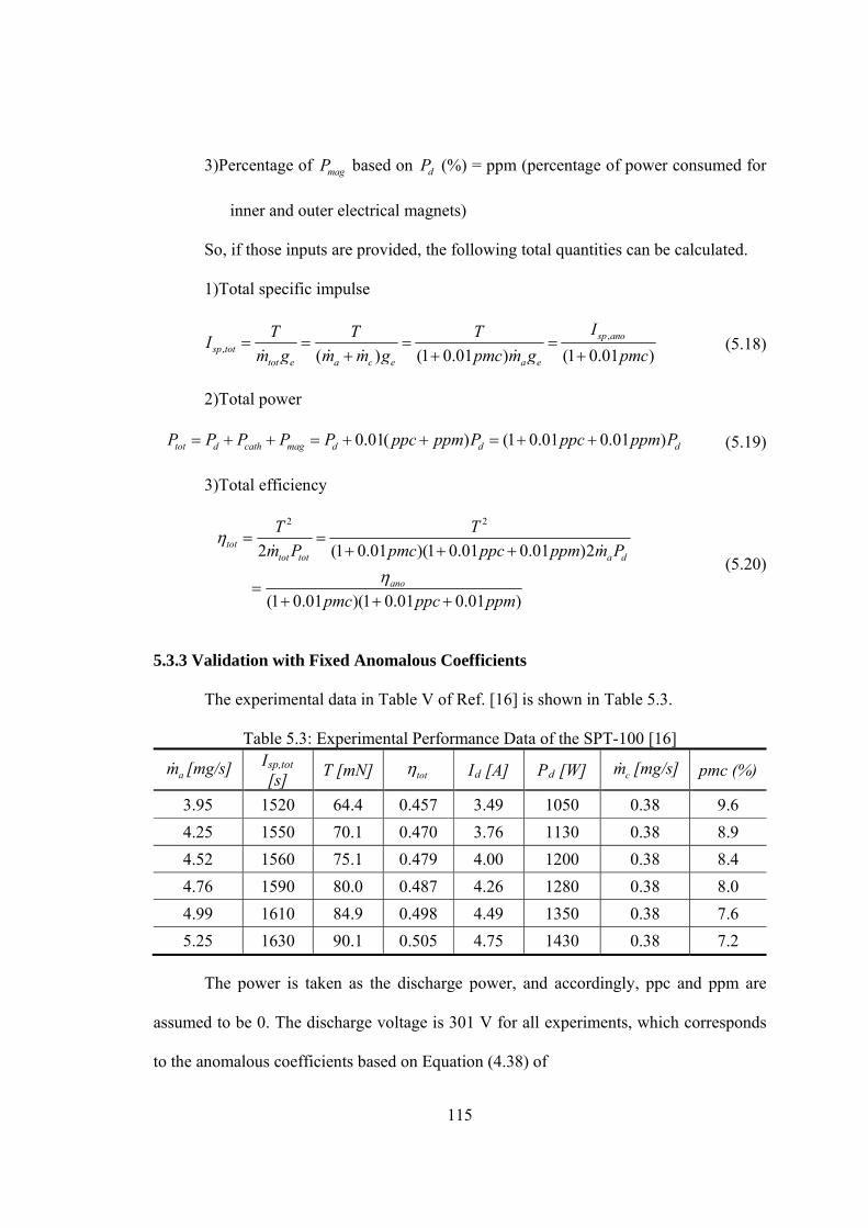
115
3)Percentage of magP based on dP (%) = ppm (percentage of power consumed for
inner and outer electrical magnets)
So, if those inputs are provided, the following total quantities can be calculated.
1)Total specific impulse
,, ( ) (1 0.01 ) (1 0.01 )
sp anosp tot
tot e a c e a e
IT T TI
m g m m g pmc m g pmc
(5.18)
2)Total power
0.01( ) (1 0.01 0.01 )tot d cath mag d d dP P P P P ppc ppm P ppc ppm P (5.19)
3)Total efficiency
2 2
2 (1 0.01 )(1 0.01 0.01 )2
(1 0.01 )(1 0.01 0.01 )
tottot tot a d
ano
T T
m P pmc ppc ppm m P
pmc ppc ppm
(5.20)
5.3.3 Validation with Fixed Anomalous Coefficients
The experimental data in Table V of Ref. [16] is shown in Table 5.3.
Table 5.3: Experimental Performance Data of the SPT-100 [16]
am [mg/s] IRsp,totR [s]
T [mN] tot IRdR [A] PRdR [W] cm [mg/s] pmc (%)
3.95 1520 64.4 0.457 3.49 1050 0.38 9.6
4.25 1550 70.1 0.470 3.76 1130 0.38 8.9
4.52 1560 75.1 0.479 4.00 1200 0.38 8.4
4.76 1590 80.0 0.487 4.26 1280 0.38 8.0
4.99 1610 84.9 0.498 4.49 1350 0.38 7.6
5.25 1630 90.1 0.505 4.75 1430 0.38 7.2
The power is taken as the discharge power, and accordingly, ppc and ppm are
assumed to be 0. The discharge voltage is 301 V for all experiments, which corresponds
to the anomalous coefficients based on Equation (4.38) of
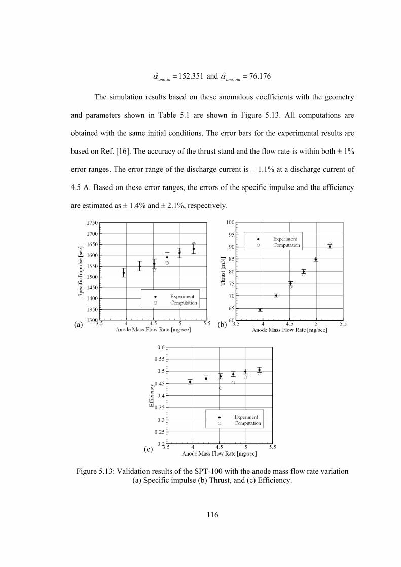
116
,ˆ 152.351ano in and ,
ˆ 76.176ano out
The simulation results based on these anomalous coefficients with the geometry
and parameters shown in Table 5.1 are shown in Figure 5.13. All computations are
obtained with the same initial conditions. The error bars for the experimental results are
based on Ref. [16]. The accuracy of the thrust stand and the flow rate is within both ± 1%
error ranges. The error range of the discharge current is ± 1.1% at a discharge current of
4.5 A. Based on these error ranges, the errors of the specific impulse and the efficiency
are estimated as ± 1.4% and ± 2.1%, respectively.
Figure 5.13: Validation results of the SPT-100 with the anode mass flow rate variation (a) Specific impulse (b) Thrust, and (c) Efficiency.
(b)(a)
(c)
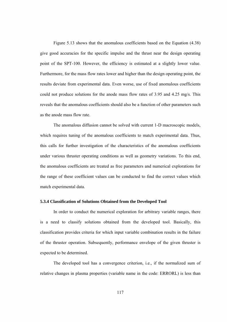
117
Figure 5.13 shows that the anomalous coefficients based on the Equation (4.38)
give good accuracies for the specific impulse and the thrust near the design operating
point of the SPT-100. However, the efficiency is estimated at a slightly lower value.
Furthermore, for the mass flow rates lower and higher than the design operating point, the
results deviate from experimental data. Even worse, use of fixed anomalous coefficients
could not produce solutions for the anode mass flow rates of 3.95 and 4.25 mg/s. This
reveals that the anomalous coefficients should also be a function of other parameters such
as the anode mass flow rate.
The anomalous diffusion cannot be solved with current 1-D macroscopic models,
which requires tuning of the anomalous coefficients to match experimental data. Thus,
this calls for further investigation of the characteristics of the anomalous coefficients
under various thruster operating conditions as well as geometry variations. To this end,
the anomalous coefficients are treated as free parameters and numerical explorations for
the range of these coefficient values can be conducted to find the correct values which
match experimental data.
5.3.4 Classification of Solutions Obtained from the Developed Tool
In order to conduct the numerical exploration for arbitrary variable ranges, there
is a need to classify solutions obtained from the developed tool. Basically, this
classification provides criteria for which input variable combination results in the failure
of the thruster operation. Subsequently, performance envelope of the given thruster is
expected to be determined.
The developed tool has a convergence criterion, i.e., if the normalized sum of
relative changes in plasma properties (variable name in the code: ERRORL) is less than
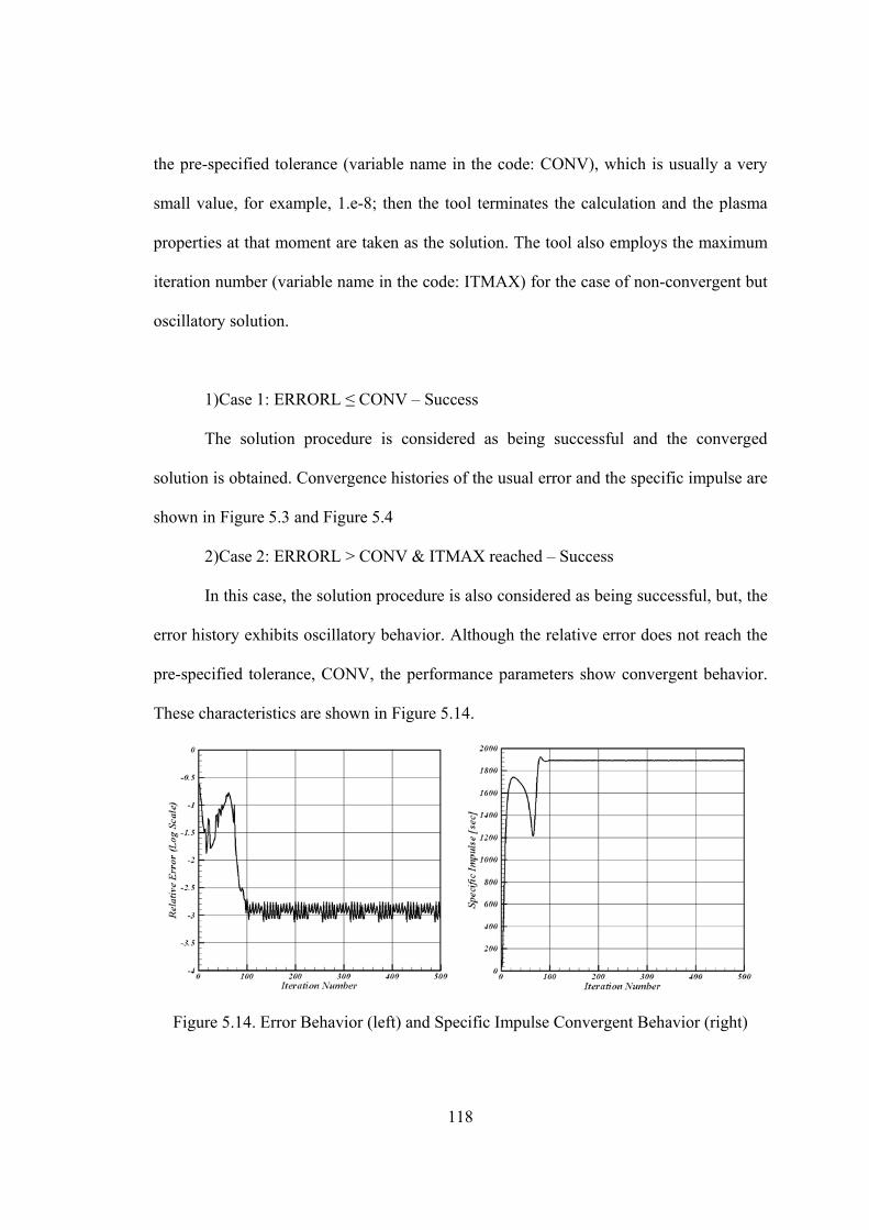
118
the pre-specified tolerance (variable name in the code: CONV), which is usually a very
small value, for example, 1.e-8; then the tool terminates the calculation and the plasma
properties at that moment are taken as the solution. The tool also employs the maximum
iteration number (variable name in the code: ITMAX) for the case of non-convergent but
oscillatory solution.
1)Case 1: ERRORL ≤ CONV – Success
The solution procedure is considered as being successful and the converged
solution is obtained. Convergence histories of the usual error and the specific impulse are
shown in Figure 5.3 and Figure 5.4
2)Case 2: ERRORL > CONV & ITMAX reached – Success
In this case, the solution procedure is also considered as being successful, but, the
error history exhibits oscillatory behavior. Although the relative error does not reach the
pre-specified tolerance, CONV, the performance parameters show convergent behavior.
These characteristics are shown in Figure 5.14.
Figure 5.14. Error Behavior (left) and Specific Impulse Convergent Behavior (right)
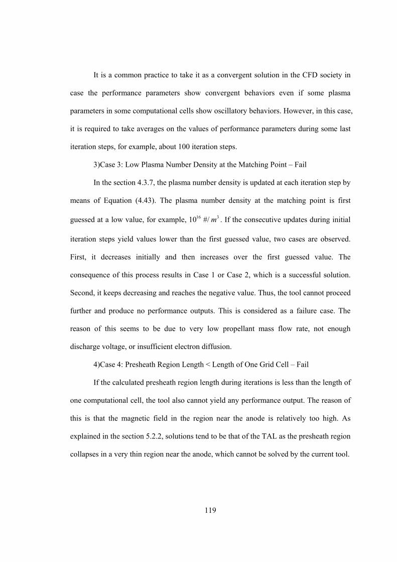
119
It is a common practice to take it as a convergent solution in the CFD society in
case the performance parameters show convergent behaviors even if some plasma
parameters in some computational cells show oscillatory behaviors. However, in this case,
it is required to take averages on the values of performance parameters during some last
iteration steps, for example, about 100 iteration steps.
3)Case 3: Low Plasma Number Density at the Matching Point – Fail
In the section 4.3.7, the plasma number density is updated at each iteration step by
means of Equation (4.43). The plasma number density at the matching point is first
guessed at a low value, for example, 16 310 #/ m . If the consecutive updates during initial
iteration steps yield values lower than the first guessed value, two cases are observed.
First, it decreases initially and then increases over the first guessed value. The
consequence of this process results in Case 1 or Case 2, which is a successful solution.
Second, it keeps decreasing and reaches the negative value. Thus, the tool cannot proceed
further and produce no performance outputs. This is considered as a failure case. The
reason of this seems to be due to very low propellant mass flow rate, not enough
discharge voltage, or insufficient electron diffusion.
4)Case 4: Presheath Region Length < Length of One Grid Cell – Fail
If the calculated presheath region length during iterations is less than the length of
one computational cell, the tool also cannot yield any performance output. The reason of
this is that the magnetic field in the region near the anode is relatively too high. As
explained in the section 5.2.2, solutions tend to be that of the TAL as the presheath region
collapses in a very thin region near the anode, which cannot be solved by the current tool.

120
This case is actually not a failure case. The developed tool simply cannot
recognize a noticeable presheath region in the macroscopic scale. However, in this
research scope, the noticeable presheath existence in the HETs should be guaranteed. The
magnetic field profile should have sufficiently low radial magnetic field strength in the
region near the anode. Because the magnetic field profile may be constructed in this way
in the view of design, this case is classified as a failure case to avoid a large magnetic
field strength near the anode region.
5)Case 5: Positive Electron Mean Velocity at the Cathode – Fail
In this case, the electron mean velocity at the cathode is positive during iteration
steps, which means that electrons exit from the thruster. If this happens, the electron
temperature in the region near the cathode will be negative, which prevent the tool from
proceeding to the solution. There are several possibilities for this occurrence. First, the
thruster might require more voltage difference between the anode and the cathode, since
the electric potential profile exhibits decreasing and increasing behavior near the cathode.
Second, electron mobility might not be enough due to low electron temperature.
6)Case 6: Presheath Region Length > Thruster Device Length – Fail
Basically, the reason seems to be similar to those for the Case 5. Particularly, the
fact that electron temperature at the matching point might be too low (cold plasma)
causes this failure.
Based on observations of many numerical experiments on the failure cases, Case
3 is the most dominant factor, which clearly indicates that certain input combinations
cannot achieve discharge phenomenon for the given thruster. Case 3 through Case 6 stops
121
the solution procedure. Because these are occurring during the iteration steps, it should be
checked whether the exact causes of failure cases are physical or numerical. This requires
intensive validation with a variety of existing thrusters.
5.3.5 Construction of Design of Experiment (DOE) Environment
In order to investigate the effects of the anomalous coefficient variation, the
environment of design of experiments is created using ModelCenterP
TMP. Figure 5.15
shows the created environment. The left figure is the component tree view, which
includes inputs and outputs for each component. The right figure shows actual linkage
between components. The “hall1d” component is an actual performance calculation
module, which corresponds to the developed tool. Inputs are information on propellant,
power, magnetic field profile, geometry, parameters for computation, and other options.
Outputs are performance, matching point properties, continuity check, maximum values,
and so forth.
The “WidthDelB” component is a simple one where the outer radius is calculated
with the given inner radius and the channel width, and maximum magnetic field strength
is obtained with the given cathode magnetic field strength and the difference between
them. This component is required because the “hall1d” module takes the inner radius and
the maximum magnetic field strength as inputs. This component is also necessary to have
the channel width and the magnetic field strength difference between the channel exit and
the cathode as variables in the design space exploration, which provides the more square-
like design space for these variables than using the outer radius, the maximum magnetic
field strength, and constraints regarding the inner radius and the cathode magnetic field.
The “PerfDetail” component is another simple one where the total performance
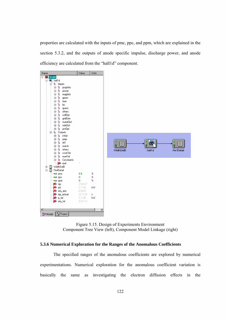
122
properties are calculated with the inputs of pmc, ppc, and ppm, which are explained in the
section 5.3.2, and the outputs of anode specific impulse, discharge power, and anode
efficiency are calculated from the “hall1d” component.
Figure 5.15. Design of Experiments Environment Component Tree View (left), Component Model Linkage (right)
5.3.6 Numerical Exploration for the Ranges of the Anomalous Coefficients
The specified ranges of the anomalous coefficients are explored by numerical
experimentations. Numerical exploration for the anomalous coefficient variation is
basically the same as investigating the electron diffusion effects in the
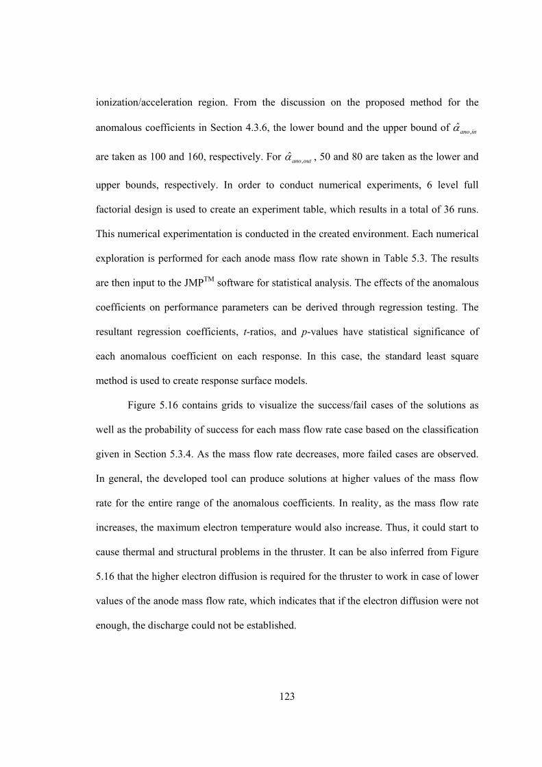
123
ionization/acceleration region. From the discussion on the proposed method for the
anomalous coefficients in Section 4.3.6, the lower bound and the upper bound of ,ˆ
ano in
are taken as 100 and 160, respectively. For ,ˆ
ano out , 50 and 80 are taken as the lower and
upper bounds, respectively. In order to conduct numerical experiments, 6 level full
factorial design is used to create an experiment table, which results in a total of 36 runs.
This numerical experimentation is conducted in the created environment. Each numerical
exploration is performed for each anode mass flow rate shown in Table 5.3. The results
are then input to the JMPP
TMP software for statistical analysis. The effects of the anomalous
coefficients on performance parameters can be derived through regression testing. The
resultant regression coefficients, t-ratios, and p-values have statistical significance of
each anomalous coefficient on each response. In this case, the standard least square
method is used to create response surface models.
Figure 5.16 contains grids to visualize the success/fail cases of the solutions as
well as the probability of success for each mass flow rate case based on the classification
given in Section 5.3.4. As the mass flow rate decreases, more failed cases are observed.
In general, the developed tool can produce solutions at higher values of the mass flow
rate for the entire range of the anomalous coefficients. In reality, as the mass flow rate
increases, the maximum electron temperature would also increase. Thus, it could start to
cause thermal and structural problems in the thruster. It can be also inferred from Figure
5.16 that the higher electron diffusion is required for the thruster to work in case of lower
values of the anode mass flow rate, which indicates that if the electron diffusion were not
enough, the discharge could not be established.
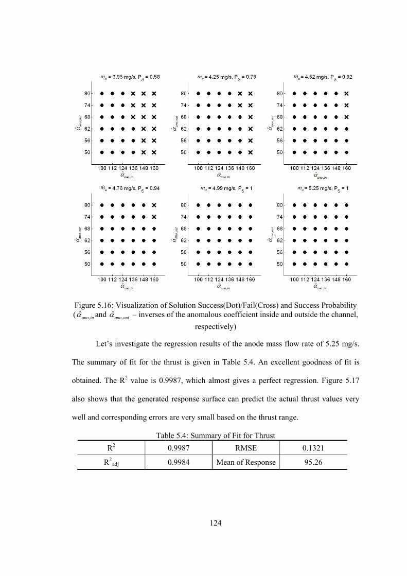
124
Figure 5.16: Visualization of Solution Success(Dot)/Fail(Cross) and Success Probability ( ,ˆano in and ,ˆano out – inverses of the anomalous coefficient inside and outside the channel,
respectively)
Let’s investigate the regression results of the anode mass flow rate of 5.25 mg/s.
The summary of fit for the thrust is given in Table 5.4. An excellent goodness of fit is
obtained. The RP
2P value is 0.9987, which almost gives a perfect regression. Figure 5.17
also shows that the generated response surface can predict the actual thrust values very
well and corresponding errors are very small based on the thrust range.
Table 5.4: Summary of Fit for Thrust
RP
2 0.9987 RMSE 0.1321
RP
2PRadj 0.9984 Mean of Response 95.26
125
Thr
ust A
ctua
l [m
N]
Thrust Predicted [mN] Thrust Predicted [mN]
Thr
ust
Res
idua
l [m
N]
Figure 5.17: Actual by Predicted (left) and Residual by Predicted (right) Plots for Thrust
Table 5.5 shows the parameter estimates and the Pareto plot. The anomalous
coefficient inside the channel plays a dominant role for thrust variation. Although the
effect of the square term of the inside anomalous coefficient is 10P
-3P times less, it is
statistically significant based on the p-value (Prob>|t|). The total specific impulse shows
the same trend as the thrust.
Table 5.5: Parameter Estimates and Associated Pareto Plot for Thrust
Term Estimate t Ratio Prob>|t| Pareto Plot
,ˆ
ano in -0.1585 -147.5 <.0001*
,ˆ
ano out -0.0256 -11.9 <.0001*
( ,ˆ
ano in -130)×( ,ˆ
ano in -130) -0.0007 -11.3 <.0001*
( ,ˆ
ano in -130)×( ,ˆ
ano out -65) 0.00019 1.9 0.0725
( ,ˆ
ano out -65)×( ,ˆ
ano out -65) 0.00022 0.9 0.3698
The anomalous coefficients are expected to have a large influence on the
discharge current because they basically control the electron cross field transport and
accordingly the axial current as seen in Table 5.6. All terms are statistically significant.
The total efficiency shows more interesting features. The goodness of fit is not as good as
those of other responses as seen in Table 5.7 and Figure 5.18, although it still shows a
high R P
2P value.
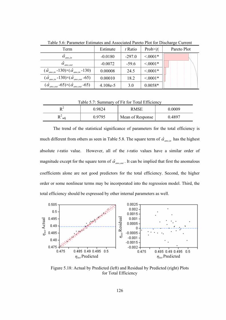
126
Table 5.6: Parameter Estimates and Associated Pareto Plot for Discharge Current
Term Estimate t Ratio Prob>|t| Pareto Plot
,ˆ
ano in -0.0180 -297.0 <.0001*
,ˆ
ano out -0.0072 -59.6 <.0001*
( ,ˆ
ano in -130)×( ,ˆ
ano in -130) 0.00008 24.5 <.0001*
( ,ˆ
ano in -130)×( ,ˆ
ano out -65) 0.00010 18.2 <.0001*
( ,ˆ
ano out -65)×( ,ˆ
ano out -65) 4.108e-5 3.0 0.0058*
Table 5.7: Summary of Fit for Total Efficiency
RP
2 0.9824 RMSE 0.0009
RP
2PRadj 0.9795 Mean of Response 0.4897
The trend of the statistical significance of parameters for the total efficiency is
much different from others as seen in Table 5.8. The square term of ,ˆ
ano in has the highest
absolute t-ratio value. However, all of the t-ratio values have a similar order of
magnitude except for the square term of ,ˆ
ano out . It can be implied that first the anomalous
coefficients alone are not good predictors for the total efficiency. Second, the higher
order or some nonlinear terms may be incorporated into the regression model. Third, the
total efficiency should be expressed by other internal parameters as well.
η tot
Act
ual
ηtot Predicted
ηtot Predicted
η tot
Res
idua
l
Figure 5.18: Actual by Predicted (left) and Residual by Predicted (right) Plots for Total Efficiency
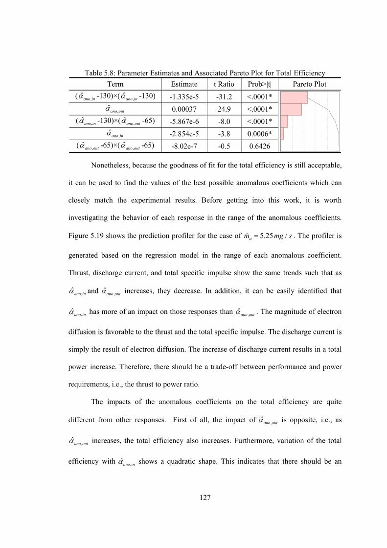
127
Table 5.8: Parameter Estimates and Associated Pareto Plot for Total Efficiency
Term Estimate t Ratio Prob>|t| Pareto Plot
( ,ˆ
ano in -130)×( ,ˆ
ano in -130) -1.335e-5 -31.2 <.0001*
,ˆ
ano out 0.00037 24.9 <.0001*
( ,ˆ
ano in -130)×( ,ˆ
ano out -65) -5.867e-6 -8.0 <.0001*
,ˆ
ano in -2.854e-5 -3.8 0.0006*
( ,ˆ
ano out -65)×( ,ˆ
ano out -65) -8.02e-7 -0.5 0.6426
Nonetheless, because the goodness of fit for the total efficiency is still acceptable,
it can be used to find the values of the best possible anomalous coefficients which can
closely match the experimental results. Before getting into this work, it is worth
investigating the behavior of each response in the range of the anomalous coefficients.
Figure 5.19 shows the prediction profiler for the case of 5.25 /am mg s . The profiler is
generated based on the regression model in the range of each anomalous coefficient.
Thrust, discharge current, and total specific impulse show the same trends such that as
,ˆ
ano in and ,ˆ
ano out increases, they decrease. In addition, it can be easily identified that
,ˆ
ano in has more of an impact on those responses than ,ˆ
ano out . The magnitude of electron
diffusion is favorable to the thrust and the total specific impulse. The discharge current is
simply the result of electron diffusion. The increase of discharge current results in a total
power increase. Therefore, there should be a trade-off between performance and power
requirements, i.e., the thrust to power ratio.
The impacts of the anomalous coefficients on the total efficiency are quite
different from other responses. First of all, the impact of ,ˆano out is opposite, i.e., as
,ˆ
ano out increases, the total efficiency also increases. Furthermore, variation of the total
efficiency with ,ˆ
ano in shows a quadratic shape. This indicates that there should be an
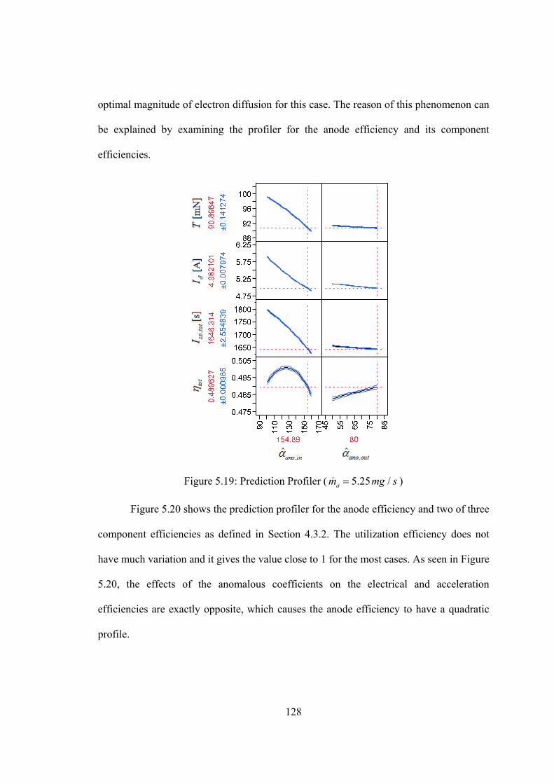
128
optimal magnitude of electron diffusion for this case. The reason of this phenomenon can
be explained by examining the profiler for the anode efficiency and its component
efficiencies.
Figure 5.19: Prediction Profiler ( 5.25 /am mg s )
Figure 5.20 shows the prediction profiler for the anode efficiency and two of three
component efficiencies as defined in Section 4.3.2. The utilization efficiency does not
have much variation and it gives the value close to 1 for the most cases. As seen in Figure
5.20, the effects of the anomalous coefficients on the electrical and acceleration
efficiencies are exactly opposite, which causes the anode efficiency to have a quadratic
profile.
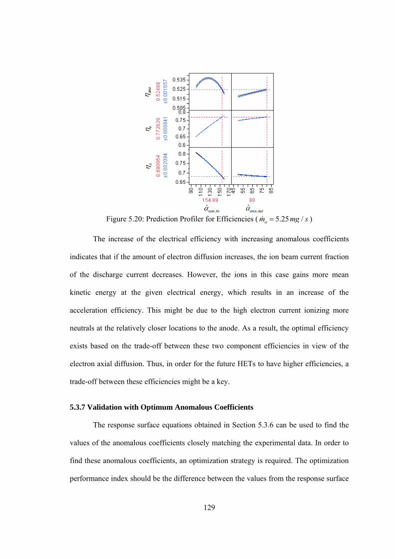
129
Figure 5.20: Prediction Profiler for Efficiencies ( 5.25 /am mg s )
The increase of the electrical efficiency with increasing anomalous coefficients
indicates that if the amount of electron diffusion increases, the ion beam current fraction
of the discharge current decreases. However, the ions in this case gains more mean
kinetic energy at the given electrical energy, which results in an increase of the
acceleration efficiency. This might be due to the high electron current ionizing more
neutrals at the relatively closer locations to the anode. As a result, the optimal efficiency
exists based on the trade-off between these two component efficiencies in view of the
electron axial diffusion. Thus, in order for the future HETs to have higher efficiencies, a
trade-off between these efficiencies might be a key.
5.3.7 Validation with Optimum Anomalous Coefficients
The response surface equations obtained in Section 5.3.6 can be used to find the
values of the anomalous coefficients closely matching the experimental data. In order to
find these anomalous coefficients, an optimization strategy is required. The optimization
performance index should be the difference between the values from the response surface
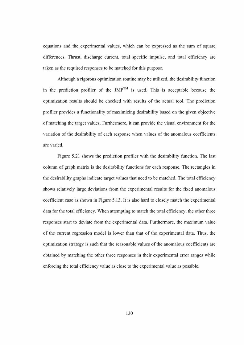
130
equations and the experimental values, which can be expressed as the sum of square
differences. Thrust, discharge current, total specific impulse, and total efficiency are
taken as the required responses to be matched for this purpose.
Although a rigorous optimization routine may be utilized, the desirability function
in the prediction profiler of the JMPP
TMP is used. This is acceptable because the
optimization results should be checked with results of the actual tool. The prediction
profiler provides a functionality of maximizing desirability based on the given objective
of matching the target values. Furthermore, it can provide the visual environment for the
variation of the desirability of each response when values of the anomalous coefficients
are varied.
Figure 5.21 shows the prediction profiler with the desirability function. The last
column of graph matrix is the desirability functions for each response. The rectangles in
the desirability graphs indicate target values that need to be matched. The total efficiency
shows relatively large deviations from the experimental results for the fixed anomalous
coefficient case as shown in Figure 5.13. It is also hard to closely match the experimental
data for the total efficiency. When attempting to match the total efficiency, the other three
responses start to deviate from the experimental data. Furthermore, the maximum value
of the current regression model is lower than that of the experimental data. Thus, the
optimization strategy is such that the reasonable values of the anomalous coefficients are
obtained by matching the other three responses in their experimental error ranges while
enforcing the total efficiency value as close to the experimental value as possible.
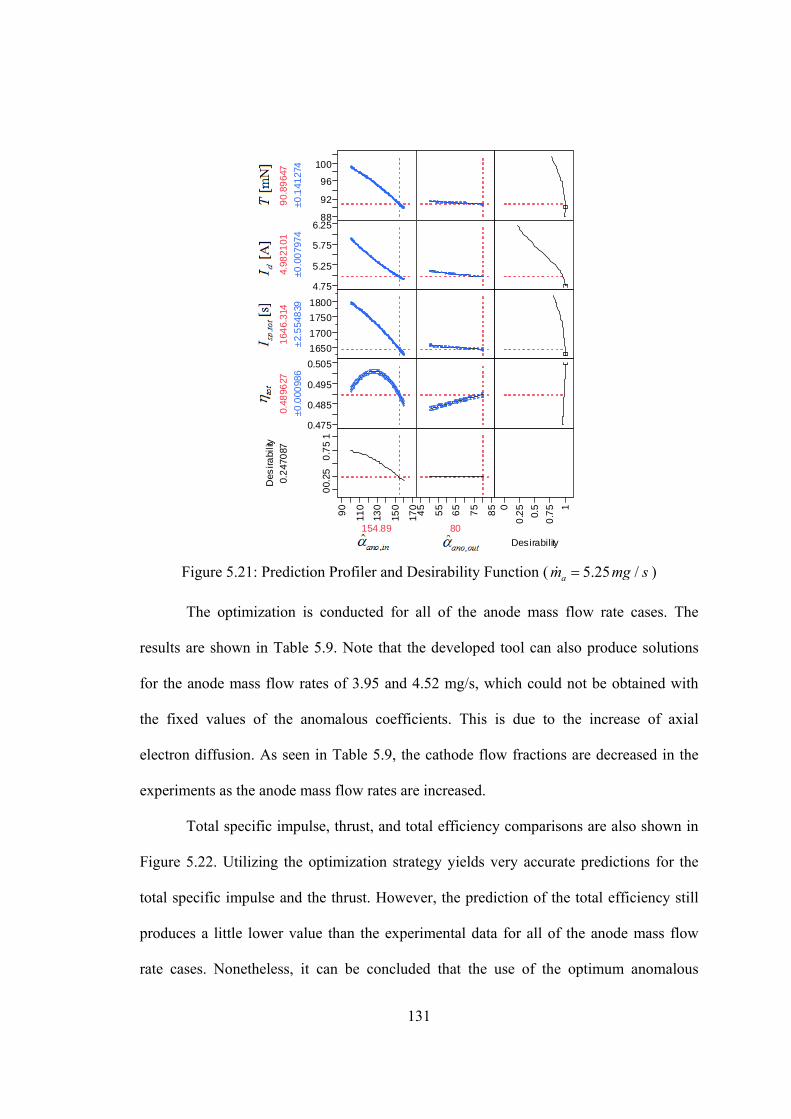
131
88
92
96
100
thru
st
90.
8964
7
±0.1
4127
44.75
5.25
5.75
6.25
id
4.98
2101
±0.0
079
74
1650
1700
1750
1800
isp_
tot
164
6.31
4
±2.
554
839
0.475
0.485
0.495
0.505
eta
_tot
0.48
9627
±0.0
0098
6
00.
250
.75
1
Des
irabi
lity
0.2
470
87
90
110
130
150
170
154.89
coe_ano1
45
55
65
75
85
80
coe_ano2
0
0.2
5
0.5
0.7
5 1
Desirability
Figure 5.21: Prediction Profiler and Desirability Function ( 5.25 /am mg s )
The optimization is conducted for all of the anode mass flow rate cases. The
results are shown in Table 5.9. Note that the developed tool can also produce solutions
for the anode mass flow rates of 3.95 and 4.52 mg/s, which could not be obtained with
the fixed values of the anomalous coefficients. This is due to the increase of axial
electron diffusion. As seen in Table 5.9, the cathode flow fractions are decreased in the
experiments as the anode mass flow rates are increased.
Total specific impulse, thrust, and total efficiency comparisons are also shown in
Figure 5.22. Utilizing the optimization strategy yields very accurate predictions for the
total specific impulse and the thrust. However, the prediction of the total efficiency still
produces a little lower value than the experimental data for all of the anode mass flow
rate cases. Nonetheless, it can be concluded that the use of the optimum anomalous
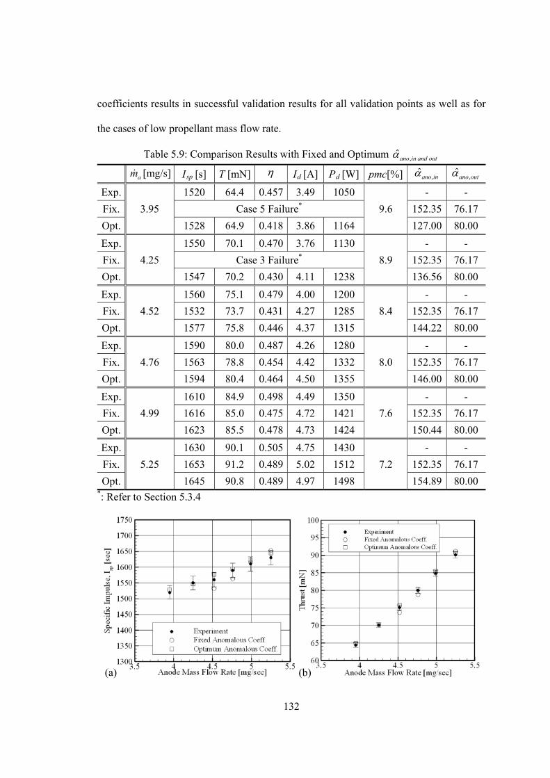
132
coefficients results in successful validation results for all validation points as well as for
the cases of low propellant mass flow rate.
Table 5.9: Comparison Results with Fixed and Optimum ,ˆ
ano in and out
am [mg/s] IRsp R[s] T [mN] IRd R[A] PRd R[W] pmc[%] ,ˆ
ano in ,ˆ
ano out
Exp.
3.95
1520 64.4 0.457 3.49 1050
9.6
- -
Fix. Case 5 FailureP
* 152.35 76.17
Opt. 1528 64.9 0.418 3.86 1164 127.00 80.00
Exp.
4.25
1550 70.1 0.470 3.76 1130
8.9
- -
Fix. Case 3 FailureP
* 152.35 76.17
Opt. 1547 70.2 0.430 4.11 1238 136.56 80.00
Exp.
4.52
1560 75.1 0.479 4.00 1200
8.4
- -
Fix. 1532 73.7 0.431 4.27 1285 152.35 76.17
Opt. 1577 75.8 0.446 4.37 1315 144.22 80.00
Exp.
4.76
1590 80.0 0.487 4.26 1280
8.0
- -
Fix. 1563 78.8 0.454 4.42 1332 152.35 76.17
Opt. 1594 80.4 0.464 4.50 1355 146.00 80.00
Exp.
4.99
1610 84.9 0.498 4.49 1350
7.6
- -
Fix. 1616 85.0 0.475 4.72 1421 152.35 76.17
Opt. 1623 85.5 0.478 4.73 1424 150.44 80.00
Exp.
5.25
1630 90.1 0.505 4.75 1430
7.2
- -
Fix. 1653 91.2 0.489 5.02 1512 152.35 76.17
Opt. 1645 90.8 0.489 4.97 1498 154.89 80.00
P
*P: Refer to Section 5.3.4
(a) (b)
133
Figure 5.22: Comparisons of Experiments, Fixed and Optimum Anomalous Coefficients (a)Total Specific Impulse (b) Thrust, and (c) Total Efficiency.
An interesting fact is that ,ˆ
ano in increases as the anode propellant mass flow rate
increases, while ,ˆ
ano out does not have much impact on the performance parameters. In
other words, the anomalous diffusion may be increased as the anode mass flow rate is
decreased. The reason for this might be the effect of the cathode propellant mass flow
rate fraction. This can be clearly seen in Figure 5.23. The cathode flow rate fraction
increases as the anode propellant mass flow rate is decreased, while ,ˆ
ano in is increased. It
seems that the anomalous coefficient inside the channel and the cathode mass flow rate
fraction are positively correlated.
In view of the actual experiments where the cathode mass flow rate is fixed as
0.38 /mg s for all cases, it is plausible that this fixed cathode mass flow rate was given
based on the lowest anode mass flow rate operation in the experiments with an intention
to establish and sustain thruster discharge at the low neutral number density operation. It
can be subsequently inferred that the increase of the cathode mass flow rate fraction
might cause a higher anomalous diffusion effect.
(c)
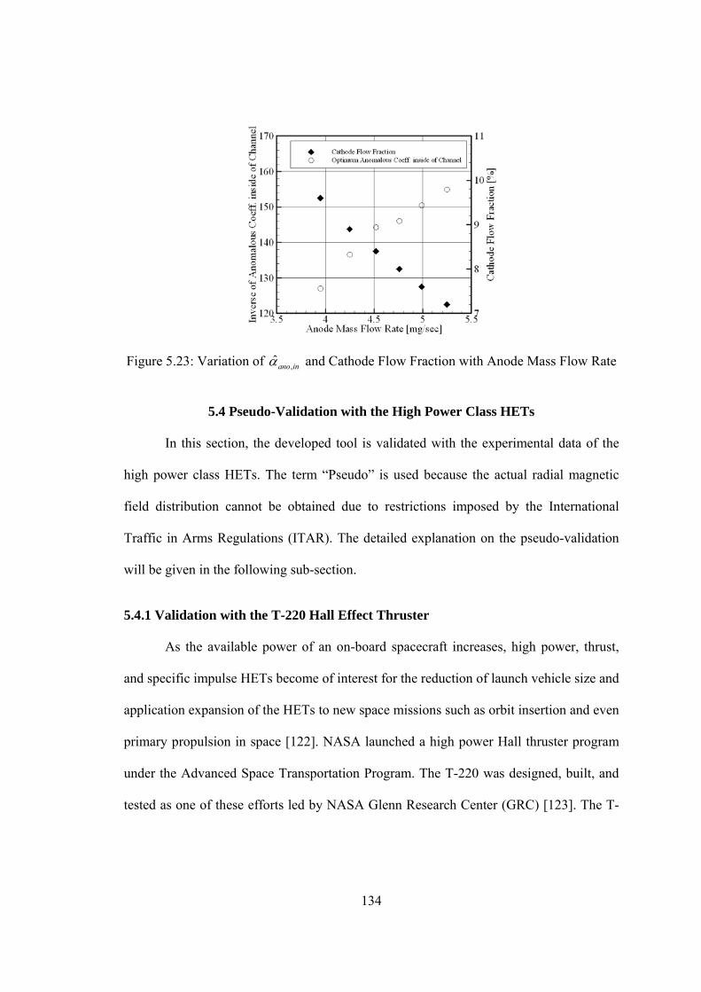
134
Figure 5.23: Variation of ,ˆ
ano in and Cathode Flow Fraction with Anode Mass Flow Rate
5.4 Pseudo-Validation with the High Power Class HETs
In this section, the developed tool is validated with the experimental data of the
high power class HETs. The term “Pseudo” is used because the actual radial magnetic
field distribution cannot be obtained due to restrictions imposed by the International
Traffic in Arms Regulations (ITAR). The detailed explanation on the pseudo-validation
will be given in the following sub-section.
5.4.1 Validation with the T-220 Hall Effect Thruster
As the available power of an on-board spacecraft increases, high power, thrust,
and specific impulse HETs become of interest for the reduction of launch vehicle size and
application expansion of the HETs to new space missions such as orbit insertion and even
primary propulsion in space [122]. NASA launched a high power Hall thruster program
under the Advanced Space Transportation Program. The T-220 was designed, built, and
tested as one of these efforts led by NASA Glenn Research Center (GRC) [123]. The T-
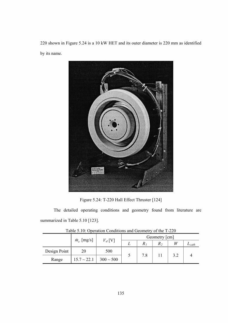
135
220 shown in Figure 5.24 is a 10 kW HET and its outer diameter is 220 mm as identified
by its name.
Figure 5.24: T-220 Hall Effect Thruster [124]
The detailed operating conditions and geometry found from literature are
summarized in Table 5.10 [123].
Table 5.10: Operation Conditions and Geometry of the T-220
am [mg/s] VRdR [V] Geometry [cm]
L RR1 RR2 W LRcath
Design Point 20 500 5 7.8 11 3.2 4
Range 15.7 ~ 22.1 300 ~ 500
136
In order to validate the developed tool with experimental data of the T-220, the
radial magnetic field distribution is required. Although it is not available from the
literature due to the ITAR Regulations, if the DOE is utilized as done in the previous
section, the approximate radial magnetic field distribution can be obtained. The approach
is a form of a reverse engineering process and the process can be generalized for other
HETs as well. This is the reason why the process is called “Pseudo-Validation.”
It is evident that pseudo-validation necessarily increases the number of numerical
experiments because parameters characterizing the radial magnetic field distribution
should be incorporated in the DOE. The radial magnetic field distribution along the
thruster axial coordinate up to the cathode can be completely determined by the three
parameters such as BRmaxR, BRcathR, and magnetic field shape coefficient inside the channel
which is denoted by K. BRmaxR and K completely determine the distribution inside the
channel by Equation (5.1). BRmaxR and BRcathR also determine the distribution outside the
channel by the assumption of linear distribution as explained in Section 5.1.1. Therefore,
variables in the DOE consist of three parameters for the magnetic field distribution and
two parameters for the anomalous coefficients.
The ranges of magnetic field variables are given in Table 5.11. In actual
numerical experimentation, ΔB is taken instead of BRmaxR because BRmaxR must be greater than
BRcathR, and it is more preferable to have a square design space in terms of the DOE. The 4
level full factorial design is created, which results in a total of 1024 runs for 5 variables.
Because there are 5 variables that have to be adjusted to match the experimental data, the
rigorous optimization routine is applied to obtain accurate results.
137
Table 5.11: Ranges of Magnetic Field Parameters
BRmaxR [T] ΔB [T] BRcathR [T] K
Lower Limit 0.015 0.005 0.010 12
Upper Limit 0.031 0.013 0.018 20
The experimental data is taken from Ref. [123]. In Ref. [123], there are two sets
of data at the design operation condition of the T-220, which differ by the measurement
date. Because there is not much difference between two data sets, the average values
from the experimental data are taken as a validation set. The results of the DOE are then
input into the JMPP
TMP to create the response surface equation for each response. The
goodness of fit is greater than 0.99 for all of the responses.
In order to find the optimum values for the anomalous coefficients and the
magnetic field distribution parameters, the “fmincon” function in MATLABP
TMP is used,
which can generally find the minimum of a constrained nonlinear multivariable function.
The normalized values in terms of median of each variable range are used and the
optimization performance index is chosen to be the sum of square errors, which are the
differences between the experimental values and the calculated values. Because the
regression equations are all quadratic and the objective function that is the sum of square
errors is also quadratic, only one step is required to find optimum values regardless of
initial conditions. The optimization results are shown in Table 5.12 with the comparison
to the experimental data and corresponding errors. The comparisons show great accuracy
and the errors are all within 2%.
The approximate radial magnetic field distribution from the optimization results is
also shown in Figure 5.25.
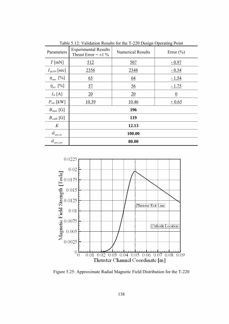
138
Table 5.12: Validation Results for the T-220 Design Operating Point
Parameters Experimental Results Thrust Error = ±1 %
Numerical Results Error (%)
T [mN] U512 U507 U- 0.97
IRsp,tot R[sec] U2356 U2348 U- 0.34
ano [%] U65 U64 U- 1.54
tot [%] U57 U56 U- 1.75
IRdR [A] U20 U20 0
PRtotR [kW] U10.39 U10.46 U+ 0.65
BRmaxR [G] 196
BRcathR [G] 119
K 12.13
,ˆano in 100.00
,ˆ
ano out 80.00
Figure 5.25: Approximate Radial Magnetic Field Distribution for the T-220
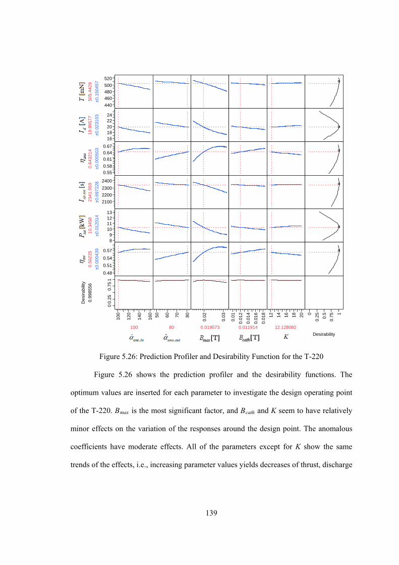
139
440
460
480
500
520th
rust
505.
4429
±0.1
5045
7
1618202224
id
19.8
9577
±0.0
2310
3
0.55
0.58
0.61
0.64
0.67
eta_
ano
0.64
3214
±0.0
0050
3
2100
2200
2300
2400
isp_
tot
2341
.959
±0.6
9722
8
89
10111213
p_to
t
10.3
458
±0.0
1201
4
0.48
0.51
0.54
0.57
eta_
tot
0.56
225
±0.0
0043
9
00.
250.
751
Des
irabi
lity
0.99
8556
100
120
140
160
100
coe_ano1
50 60 70 80
80
coe_ano2
0.02
0.03
0.019573
bmax
0.01
0.01
2
0.01
4
0.01
6
0.01
8
0.011914
bcath
12 14 16 18 20
12.128092
K
0
0.25 0.5
0.75 1
Desirability
Figure 5.26: Prediction Profiler and Desirability Function for the T-220
Figure 5.26 shows the prediction profiler and the desirability functions. The
optimum values are inserted for each parameter to investigate the design operating point
of the T-220. BRmaxR is the most significant factor, and BRcathR and K seem to have relatively
minor effects on the variation of the responses around the design point. The anomalous
coefficients have moderate effects. All of the parameters except for K show the same
trends of the effects, i.e., increasing parameter values yields decreases of thrust, discharge
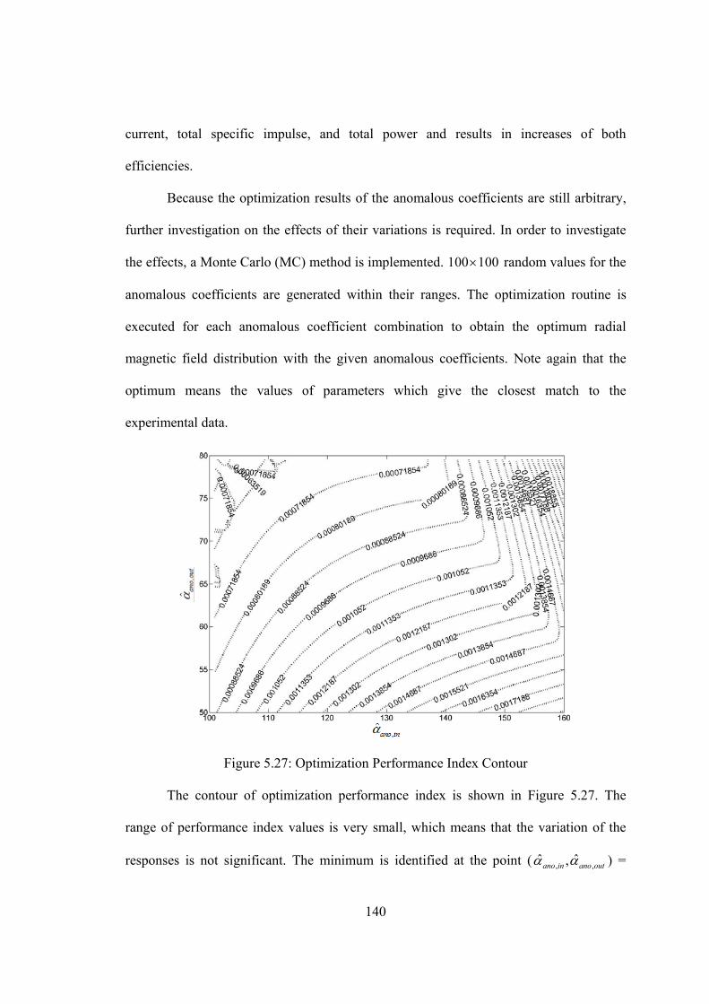
140
current, total specific impulse, and total power and results in increases of both
efficiencies.
Because the optimization results of the anomalous coefficients are still arbitrary,
further investigation on the effects of their variations is required. In order to investigate
the effects, a Monte Carlo (MC) method is implemented. 100 100 random values for the
anomalous coefficients are generated within their ranges. The optimization routine is
executed for each anomalous coefficient combination to obtain the optimum radial
magnetic field distribution with the given anomalous coefficients. Note again that the
optimum means the values of parameters which give the closest match to the
experimental data.
Figure 5.27: Optimization Performance Index Contour
The contour of optimization performance index is shown in Figure 5.27. The
range of performance index values is very small, which means that the variation of the
responses is not significant. The minimum is identified at the point ( , ,ˆ ˆ,ano in ano out ) =
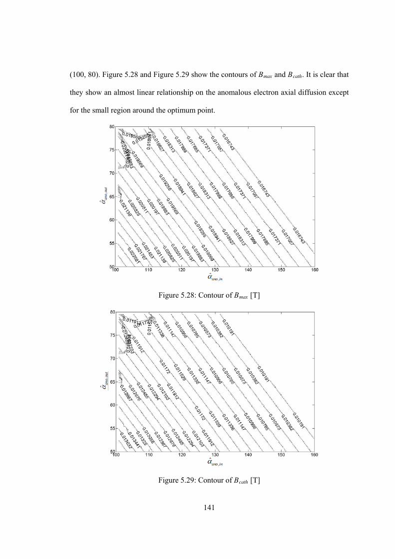
141
(100, 80). Figure 5.28 and Figure 5.29 show the contours of BRmaxR and BRcathR. It is clear that
they show an almost linear relationship on the anomalous electron axial diffusion except
for the small region around the optimum point.
Figure 5.28: Contour of BRmaxR [T]
Figure 5.29: Contour of BRcathR [T]
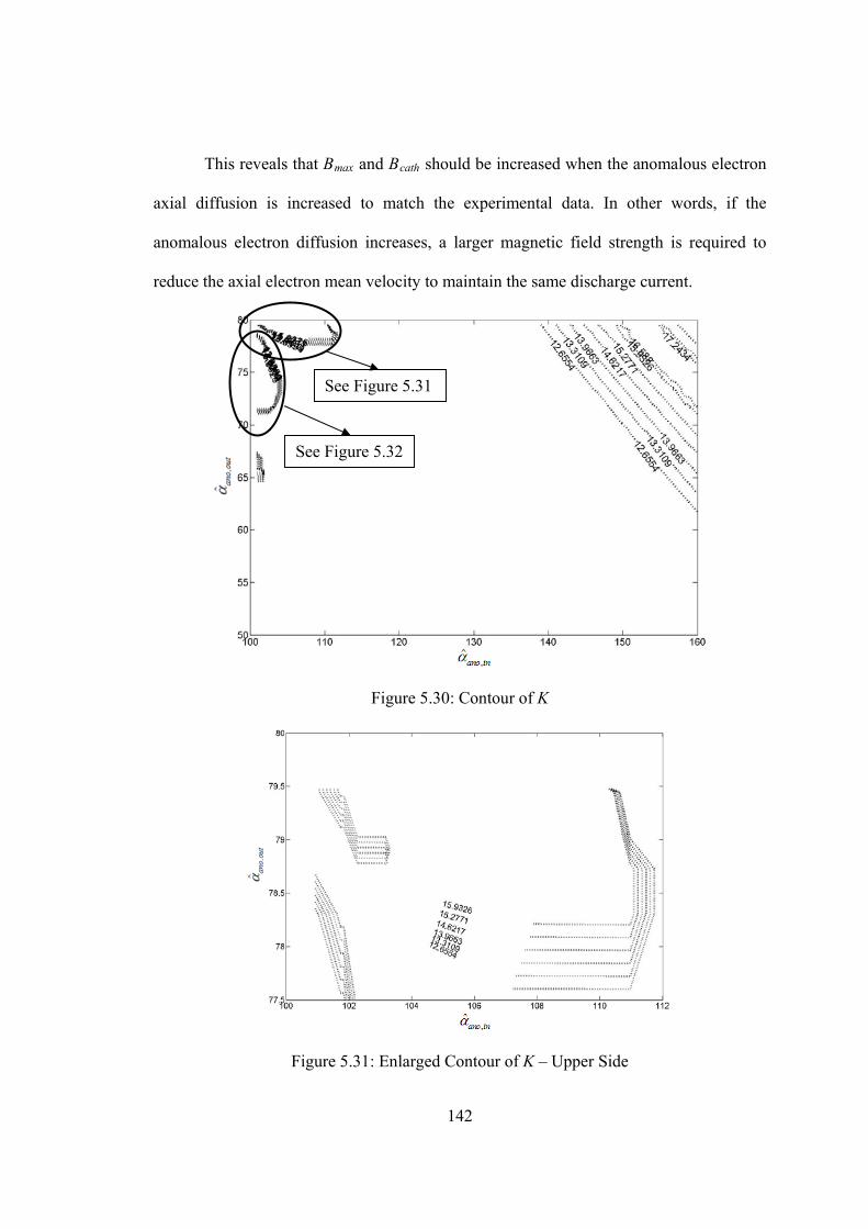
142
This reveals that BRmaxR and BRcathR should be increased when the anomalous electron
axial diffusion is increased to match the experimental data. In other words, if the
anomalous electron diffusion increases, a larger magnetic field strength is required to
reduce the axial electron mean velocity to maintain the same discharge current.
Figure 5.30: Contour of K
Figure 5.31: Enlarged Contour of K – Upper Side
See Figure 5.32
See Figure 5.31
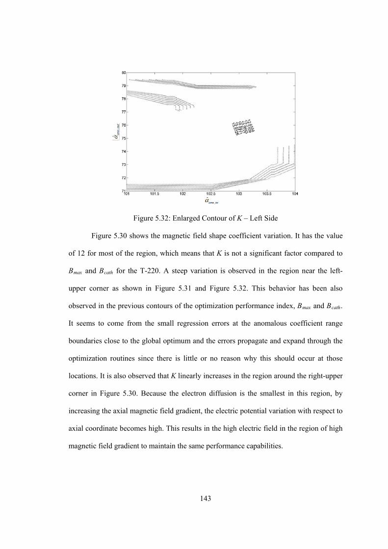
143
Figure 5.32: Enlarged Contour of K – Left Side
Figure 5.30 shows the magnetic field shape coefficient variation. It has the value
of 12 for most of the region, which means that K is not a significant factor compared to
BRmaxR and BRcathR for the T-220. A steep variation is observed in the region near the left-
upper corner as shown in Figure 5.31 and Figure 5.32. This behavior has been also
observed in the previous contours of the optimization performance index, BRmaxR and BRcathR.
It seems to come from the small regression errors at the anomalous coefficient range
boundaries close to the global optimum and the errors propagate and expand through the
optimization routines since there is little or no reason why this should occur at those
locations. It is also observed that K linearly increases in the region around the right-upper
corner in Figure 5.30. Because the electron diffusion is the smallest in this region, by
increasing the axial magnetic field gradient, the electric potential variation with respect to
axial coordinate becomes high. This results in the high electric field in the region of high
magnetic field gradient to maintain the same performance capabilities.
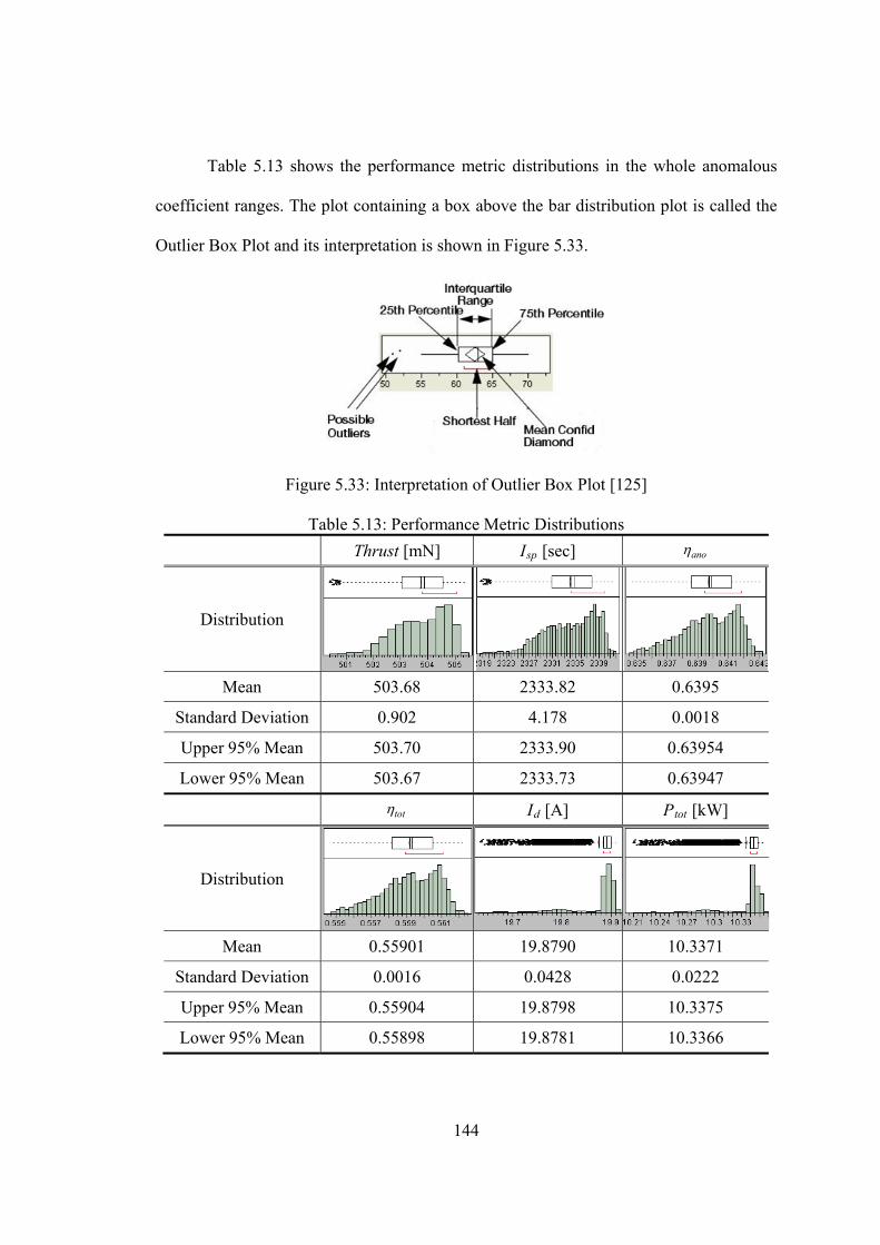
144
Table 5.13 shows the performance metric distributions in the whole anomalous
coefficient ranges. The plot containing a box above the bar distribution plot is called the
Outlier Box Plot and its interpretation is shown in Figure 5.33.
Figure 5.33: Interpretation of Outlier Box Plot [125]
Table 5.13: Performance Metric Distributions
Thrust [mN] IRspR [sec] ano
Distribution
Mean 503.68 2333.82 0.6395
Standard Deviation 0.902 4.178 0.0018
Upper 95% Mean 503.70 2333.90 0.63954
Lower 95% Mean 503.67 2333.73 0.63947
tot IRdR [A] PRtotR [kW]
Distribution
Mean 0.55901 19.8790 10.3371
Standard Deviation 0.0016 0.0428 0.0222
Upper 95% Mean 0.55904 19.8798 10.3375
Lower 95% Mean 0.55898 19.8781 10.3366
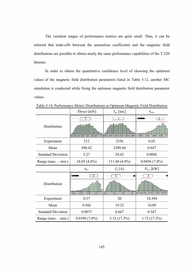
145
The variation ranges of performance metrics are quite small. Thus, it can be
inferred that trade-offs between the anomalous coefficients and the magnetic field
distributions are possible to obtain nearly the same performance capabilities of the T-220
thruster.
In order to obtain the quantitative confidence level of choosing the optimum
values of the magnetic field distribution parameters listed in Table 5.12, another MC
simulation is conducted while fixing the optimum magnetic field distribution parameter
values.
Table 5.14: Performance Metric Distributions at Optimum Magnetic Field Distribution
Thrust [mN] IRspR [sec] ano
Distribution
Experiment 512 2356 0.65
Mean 498.42 2309.44 0.647
Standard Deviation 5.27 24.42 0.0086
Range (max. – min.) 24.05 (4.8%) 111.48 (4.8%) 0.0456 (7.0%)
tot IRdR [A] PRtotR [kW]
Distribution
Experiment 0.57 20 10.394
Mean 0.566 19.22 10.00
Standard Deviation 0.0075 0.667 0.347
Range (max. – min.) 0.0398 (7.0%) 3.33 (17.3%) 1.73 (17.3%)
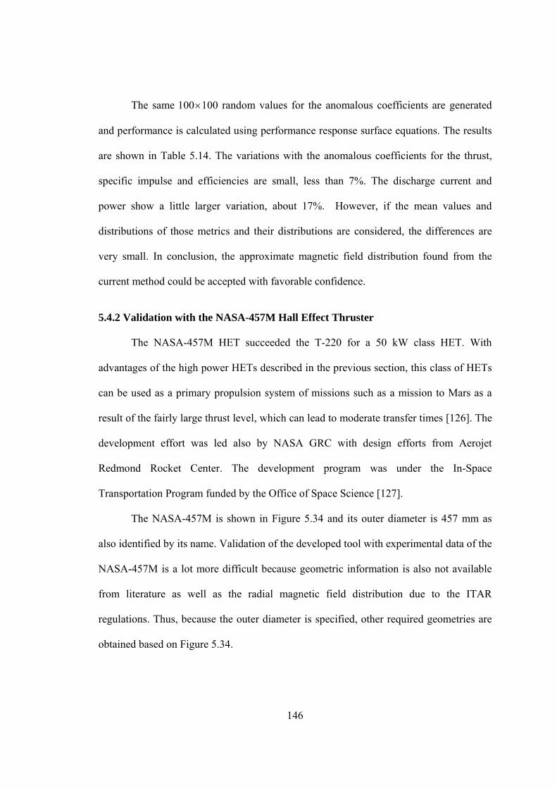
146
The same 100 100 random values for the anomalous coefficients are generated
and performance is calculated using performance response surface equations. The results
are shown in Table 5.14. The variations with the anomalous coefficients for the thrust,
specific impulse and efficiencies are small, less than 7%. The discharge current and
power show a little larger variation, about 17%. However, if the mean values and
distributions of those metrics and their distributions are considered, the differences are
very small. In conclusion, the approximate magnetic field distribution found from the
current method could be accepted with favorable confidence.
5.4.2 Validation with the NASA-457M Hall Effect Thruster
The NASA-457M HET succeeded the T-220 for a 50 kW class HET. With
advantages of the high power HETs described in the previous section, this class of HETs
can be used as a primary propulsion system of missions such as a mission to Mars as a
result of the fairly large thrust level, which can lead to moderate transfer times [126]. The
development effort was led also by NASA GRC with design efforts from Aerojet
Redmond Rocket Center. The development program was under the In-Space
Transportation Program funded by the Office of Space Science [127].
The NASA-457M is shown in Figure 5.34 and its outer diameter is 457 mm as
also identified by its name. Validation of the developed tool with experimental data of the
NASA-457M is a lot more difficult because geometric information is also not available
from literature as well as the radial magnetic field distribution due to the ITAR
regulations. Thus, because the outer diameter is specified, other required geometries are
obtained based on Figure 5.34.
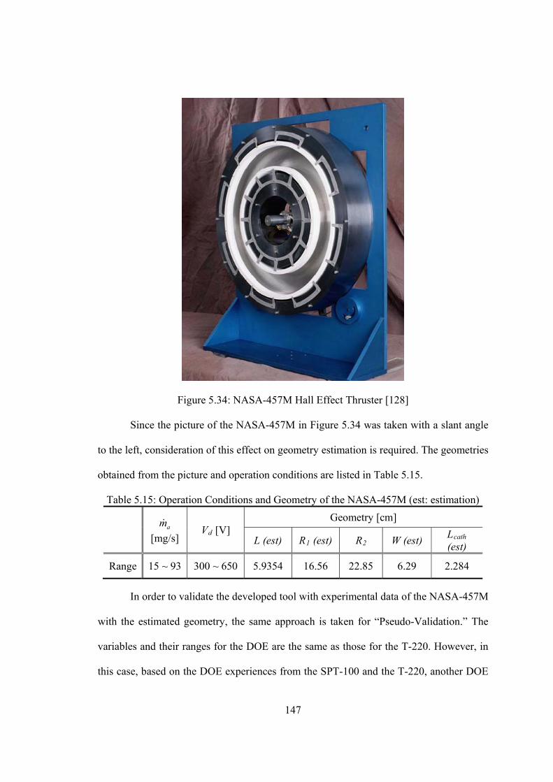
147
Figure 5.34: NASA-457M Hall Effect Thruster [128]
Since the picture of the NASA-457M in Figure 5.34 was taken with a slant angle
to the left, consideration of this effect on geometry estimation is required. The geometries
obtained from the picture and operation conditions are listed in Table 5.15.
Table 5.15: Operation Conditions and Geometry of the NASA-457M (est: estimation)
am
[mg/s] VRdR [V]
Geometry [cm]
L (est) RR1R (est) RR2 W (est) LRcathR (est)
Range 15 ~ 93 300 ~ 650 5.9354 16.56 22.85 6.29 2.284
In order to validate the developed tool with experimental data of the NASA-457M
with the estimated geometry, the same approach is taken for “Pseudo-Validation.” The
variables and their ranges for the DOE are the same as those for the T-220. However, in
this case, based on the DOE experiences from the SPT-100 and the T-220, another DOE
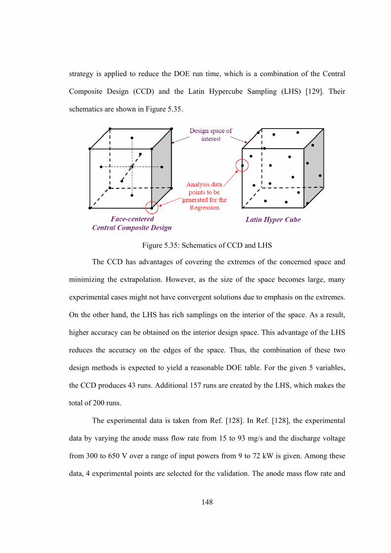
148
strategy is applied to reduce the DOE run time, which is a combination of the Central
Composite Design (CCD) and the Latin Hypercube Sampling (LHS) [129]. Their
schematics are shown in Figure 5.35.
Figure 5.35: Schematics of CCD and LHS
The CCD has advantages of covering the extremes of the concerned space and
minimizing the extrapolation. However, as the size of the space becomes large, many
experimental cases might not have convergent solutions due to emphasis on the extremes.
On the other hand, the LHS has rich samplings on the interior of the space. As a result,
higher accuracy can be obtained on the interior design space. This advantage of the LHS
reduces the accuracy on the edges of the space. Thus, the combination of these two
design methods is expected to yield a reasonable DOE table. For the given 5 variables,
the CCD produces 43 runs. Additional 157 runs are created by the LHS, which makes the
total of 200 runs.
The experimental data is taken from Ref. [128]. In Ref. [128], the experimental
data by varying the anode mass flow rate from 15 to 93 mg/s and the discharge voltage
from 300 to 650 V over a range of input powers from 9 to 72 kW is given. Among these
data, 4 experimental points are selected for the validation. The anode mass flow rate and
149
the cathode mass flow rate for all points are 74.3 mg/s and 7.5 mg/s, respectively. The
resultant percentage of the cathode mass flow rate (pmc) is then calculated as 10.09 %.
Other experimental parameters and performance metrics are shown in Table 5.16.
Table 5.16: Experimental Data of the NASA-457M [128] (Thrust Error = ± 1%) VRdR [V]
T [mN] IRsp,anoR
[s] IRsp,totR [s] ano tot IRdR [A]
PRdR [kW]
PRtotR [kW]
ppm + ppc [%]
300 1395.5 1914.5 1739 0.555 0.48 78.5 23.59 24.80 5.14
402 1688 2315 2103 0.60 0.52 80 32.14 33.45 4.05
500 1930 2648 2405 0.62 0.54 81 40.48 41.81 3.27
649 2184 2996 2722 0.62 0.55 80 51.64 52.84 2.32
The results of the DOE for the discharge voltage of 300 V show 116 failure cases
out of a total of 200 cases. For the discharge voltage of 402 V, only 4 failure cases occur.
The DOE for two other discharge voltage cases doesn’t have any failure cases. This
somewhat coincides with what’s encountered for the SPT-100. For the SPT-100, low
anode mass flow rates with low electron diffusion causes a thruster discharge failure.
Thus, it is observed for the SPT-100 that increasing the cathode mass flow rate fraction
could be one factor causing larger anomalous electron diffusion. For the current case, low
discharge voltage causes the failure. This means that the discharge voltage is also related
to the anomalous electron diffusion, which will be discussed in more detail.
From the DOE results with the developed tool, the resultant response surface
equations for each performance metrics are created using JMPP
TMP software as before.
Because the number of runs is reduced for each case compared to the T-220 cases and the
failure cases for the discharge voltage of 300 V are over half of the total runs, the
goodness of fits should be carefully checked. Table 5.17 shows the goodness of fit for
each metric at each discharge voltage. All are over 0.99 of RP
2P value except for the
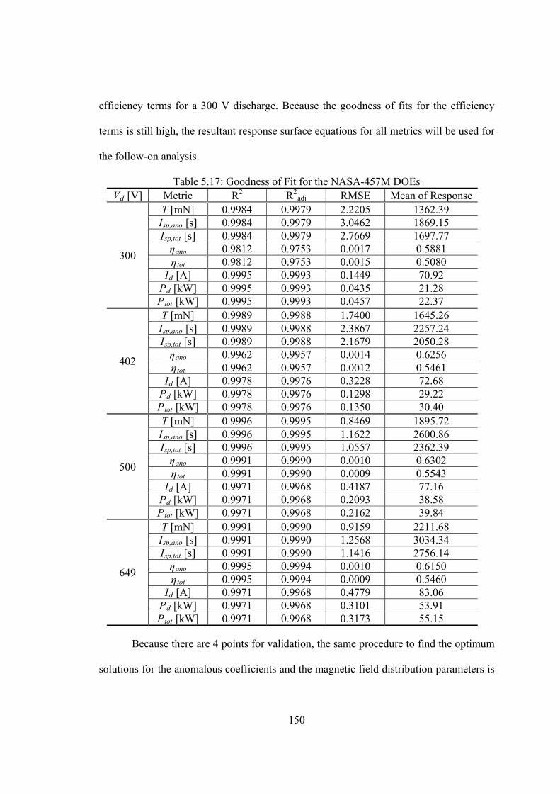
150
efficiency terms for a 300 V discharge. Because the goodness of fits for the efficiency
terms is still high, the resultant response surface equations for all metrics will be used for
the follow-on analysis.
Table 5.17: Goodness of Fit for the NASA-457M DOEs VRdR [V] Metric RP
2 RP
2PRadj RMSE Mean of Response
300
T [mN] 0.9984 0.9979 2.2205 1362.39 IRsp,anoR [s] 0.9984 0.9979 3.0462 1869.15 IRsp,totR [s] 0.9984 0.9979 2.7669 1697.77 ηRano
0.9812 0.9753 0.0017 0.5881 ηRtot
0.9812 0.9753 0.0015 0.5080 IRdR [A] 0.9995 0.9993 0.1449 70.92
PRdR [kW] 0.9995 0.9993 0.0435 21.28 PRtotR [kW] 0.9995 0.9993 0.0457 22.37
402
T [mN] 0.9989 0.9988 1.7400 1645.26 IRsp,anoR [s] 0.9989 0.9988 2.3867 2257.24 IRsp,totR [s] 0.9989 0.9988 2.1679 2050.28 ηRano
0.9962 0.9957 0.0014 0.6256 ηRtot
0.9962 0.9957 0.0012 0.5461 IRdR [A] 0.9978 0.9976 0.3228 72.68
PRdR [kW] 0.9978 0.9976 0.1298 29.22 PRtotR [kW] 0.9978 0.9976 0.1350 30.40
500
T [mN] 0.9996 0.9995 0.8469 1895.72 IRsp,anoR [s] 0.9996 0.9995 1.1622 2600.86 IRsp,totR [s] 0.9996 0.9995 1.0557 2362.39 ηRano
0.9991 0.9990 0.0010 0.6302 ηRtot
0.9991 0.9990 0.0009 0.5543 IRdR [A] 0.9971 0.9968 0.4187 77.16
PRdR [kW] 0.9971 0.9968 0.2093 38.58 PRtotR [kW] 0.9971 0.9968 0.2162 39.84
649
T [mN] 0.9991 0.9990 0.9159 2211.68 IRsp,anoR [s] 0.9991 0.9990 1.2568 3034.34 IRsp,totR [s] 0.9991 0.9990 1.1416 2756.14 ηRano
0.9995 0.9994 0.0010 0.6150 ηRtot
0.9995 0.9994 0.0009 0.5460 IRdR [A] 0.9971 0.9968 0.4779 83.06
PRdR [kW] 0.9971 0.9968 0.3101 53.91 PRtotR [kW] 0.9971 0.9968 0.3173 55.15
Because there are 4 points for validation, the same procedure to find the optimum
solutions for the anomalous coefficients and the magnetic field distribution parameters is
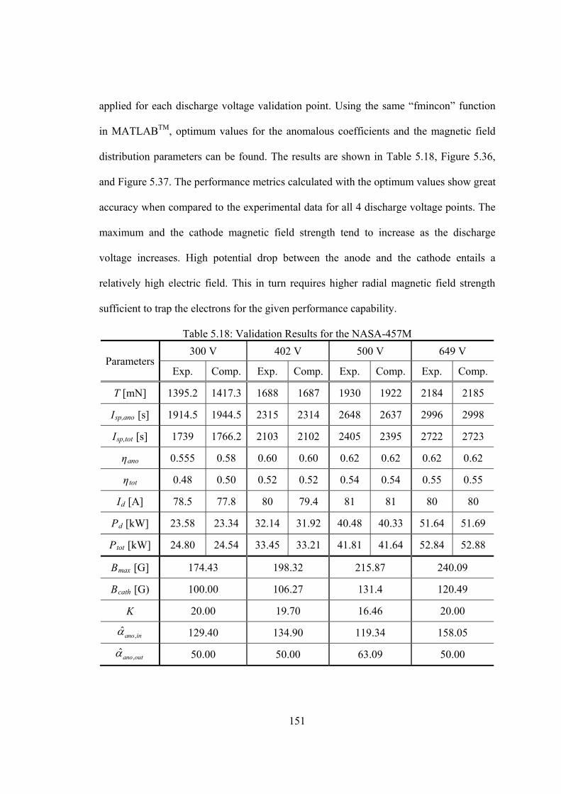
151
applied for each discharge voltage validation point. Using the same “fmincon” function
in MATLABP
TMP, optimum values for the anomalous coefficients and the magnetic field
distribution parameters can be found. The results are shown in Table 5.18, Figure 5.36,
and Figure 5.37. The performance metrics calculated with the optimum values show great
accuracy when compared to the experimental data for all 4 discharge voltage points. The
maximum and the cathode magnetic field strength tend to increase as the discharge
voltage increases. High potential drop between the anode and the cathode entails a
relatively high electric field. This in turn requires higher radial magnetic field strength
sufficient to trap the electrons for the given performance capability.
Table 5.18: Validation Results for the NASA-457M
Parameters 300 V 402 V 500 V 649 V
Exp. Comp. Exp. Comp. Exp. Comp. Exp. Comp.
T [mN] 1395.2 1417.3 1688 1687 1930 1922 2184 2185
IRsp,anoR [s] 1914.5 1944.5 2315 2314 2648 2637 2996 2998
IRsp,totR [s] 1739 1766.2 2103 2102 2405 2395 2722 2723
ηRano 0.555 0.58 0.60 0.60 0.62 0.62 0.62 0.62
ηRtot 0.48 0.50 0.52 0.52 0.54 0.54 0.55 0.55
IRdR [A] 78.5 77.8 80 79.4 81 81 80 80
PRdR [kW] 23.58 23.34 32.14 31.92 40.48 40.33 51.64 51.69
PRtotR [kW] 24.80 24.54 33.45 33.21 41.81 41.64 52.84 52.88
BRmaxR [G] 174.43 198.32 215.87 240.09
BRcathR [G) 100.00 106.27 131.4 120.49
K 20.00 19.70 16.46 20.00
,ˆ
ano in 129.40 134.90 119.34 158.05
,ˆ
ano out 50.00 50.00 63.09 50.00
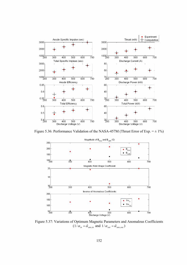
152
Figure 5.36: Performance Validation of the NASA-457M (Thrust Error of Exp. = ± 1%)
Figure 5.37: Variations of Optimum Magnetic Parameters and Anomalous Coefficients ( ,ˆ1 / in ano in and ,ˆ1 / out ano out )
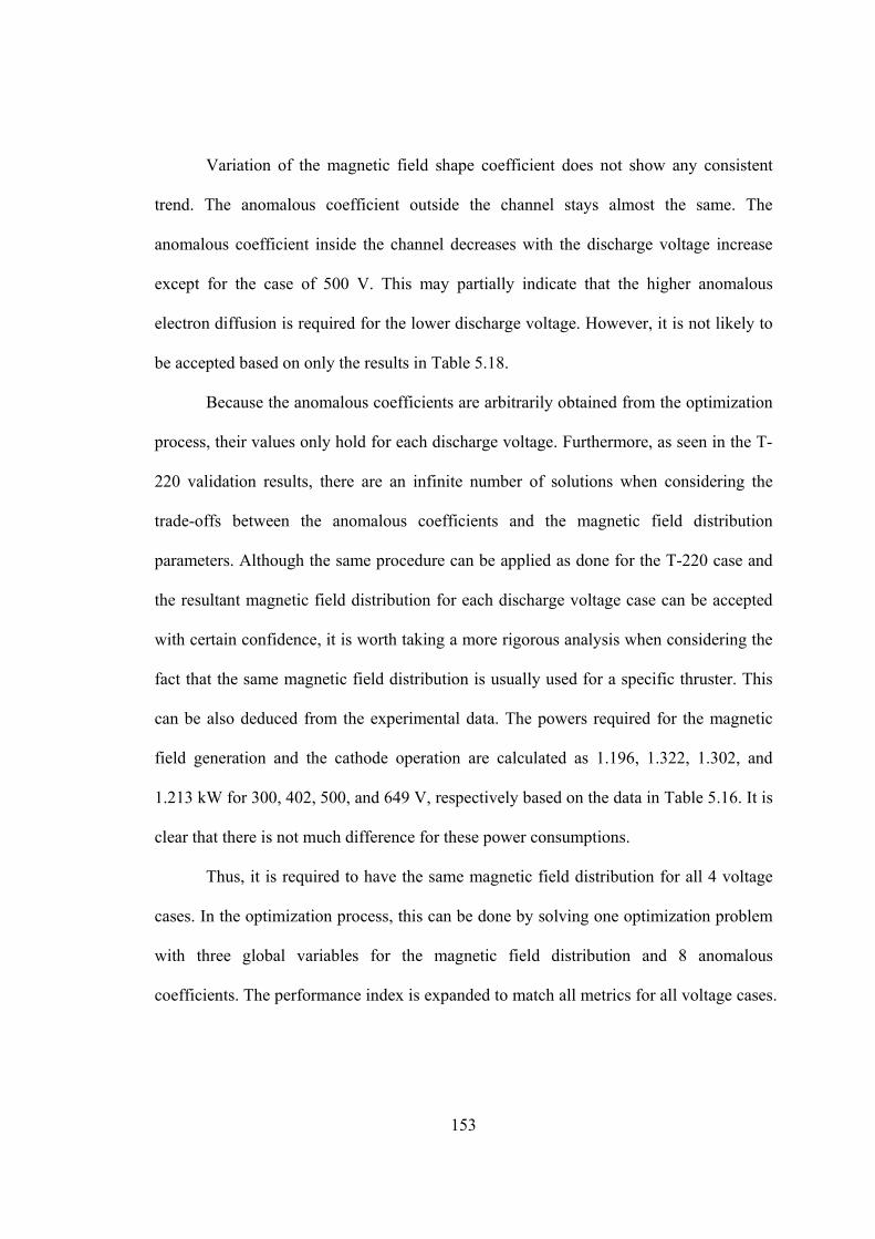
153
Variation of the magnetic field shape coefficient does not show any consistent
trend. The anomalous coefficient outside the channel stays almost the same. The
anomalous coefficient inside the channel decreases with the discharge voltage increase
except for the case of 500 V. This may partially indicate that the higher anomalous
electron diffusion is required for the lower discharge voltage. However, it is not likely to
be accepted based on only the results in Table 5.18.
Because the anomalous coefficients are arbitrarily obtained from the optimization
process, their values only hold for each discharge voltage. Furthermore, as seen in the T-
220 validation results, there are an infinite number of solutions when considering the
trade-offs between the anomalous coefficients and the magnetic field distribution
parameters. Although the same procedure can be applied as done for the T-220 case and
the resultant magnetic field distribution for each discharge voltage case can be accepted
with certain confidence, it is worth taking a more rigorous analysis when considering the
fact that the same magnetic field distribution is usually used for a specific thruster. This
can be also deduced from the experimental data. The powers required for the magnetic
field generation and the cathode operation are calculated as 1.196, 1.322, 1.302, and
1.213 kW for 300, 402, 500, and 649 V, respectively based on the data in Table 5.16. It is
clear that there is not much difference for these power consumptions.
Thus, it is required to have the same magnetic field distribution for all 4 voltage
cases. In the optimization process, this can be done by solving one optimization problem
with three global variables for the magnetic field distribution and 8 anomalous
coefficients. The performance index is expanded to match all metrics for all voltage cases.
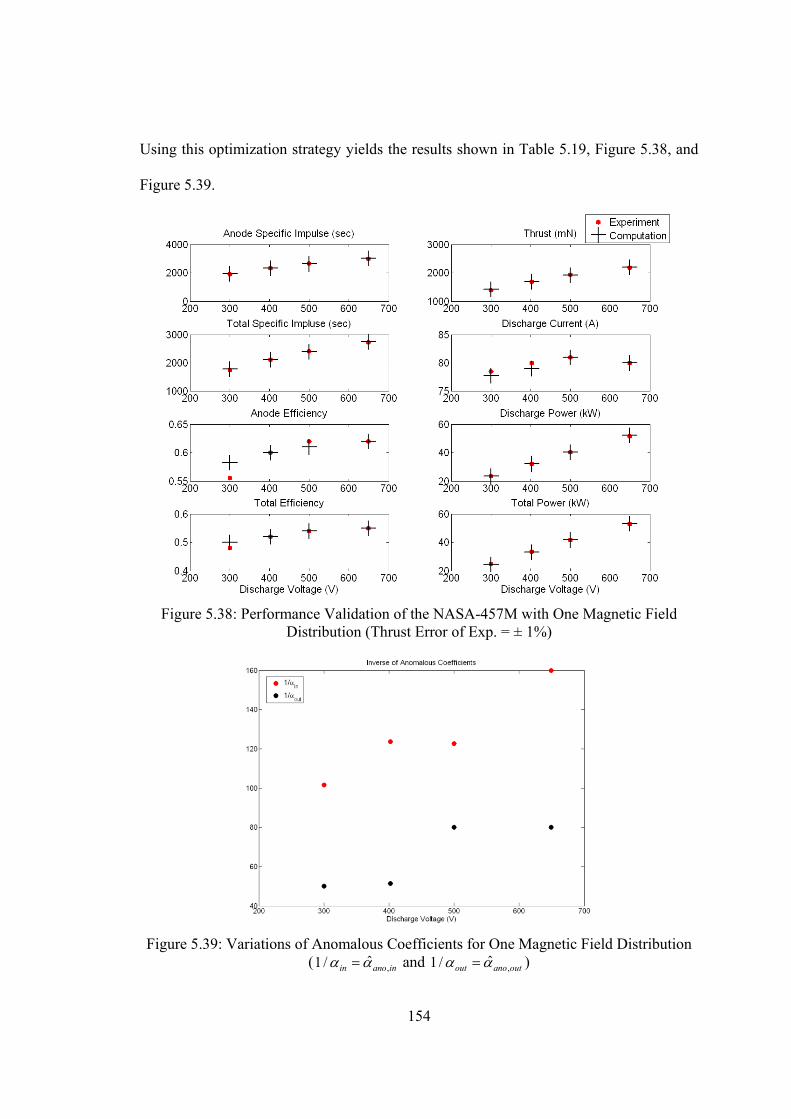
154
Using this optimization strategy yields the results shown in Table 5.19, Figure 5.38, and
Figure 5.39.
Figure 5.38: Performance Validation of the NASA-457M with One Magnetic Field Distribution (Thrust Error of Exp. = ± 1%)
Figure 5.39: Variations of Anomalous Coefficients for One Magnetic Field Distribution ( ,ˆ1 / in ano in and ,ˆ1 / out ano out )
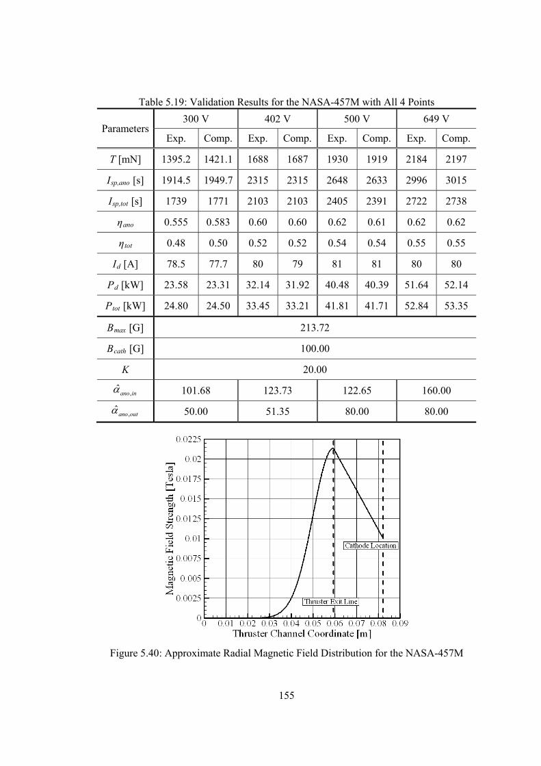
155
Table 5.19: Validation Results for the NASA-457M with All 4 Points
Parameters 300 V 402 V 500 V 649 V
Exp. Comp. Exp. Comp. Exp. Comp. Exp. Comp.
T [mN] 1395.2 1421.1 1688 1687 1930 1919 2184 2197
IRsp,anoR [s] 1914.5 1949.7 2315 2315 2648 2633 2996 3015
IRsp,totR [s] 1739 1771 2103 2103 2405 2391 2722 2738
ηRano 0.555 0.583 0.60 0.60 0.62 0.61 0.62 0.62
ηRtot 0.48 0.50 0.52 0.52 0.54 0.54 0.55 0.55
IRdR [A] 78.5 77.7 80 79 81 81 80 80
PRdR [kW] 23.58 23.31 32.14 31.92 40.48 40.39 51.64 52.14
PRtotR [kW] 24.80 24.50 33.45 33.21 41.81 41.71 52.84 53.35
BRmaxR [G] 213.72
BRcathR [G] 100.00
K 20.00
,ˆ
ano in 101.68 123.73 122.65 160.00
,ˆ
ano out 50.00 51.35 80.00 80.00
Figure 5.40: Approximate Radial Magnetic Field Distribution for the NASA-457M
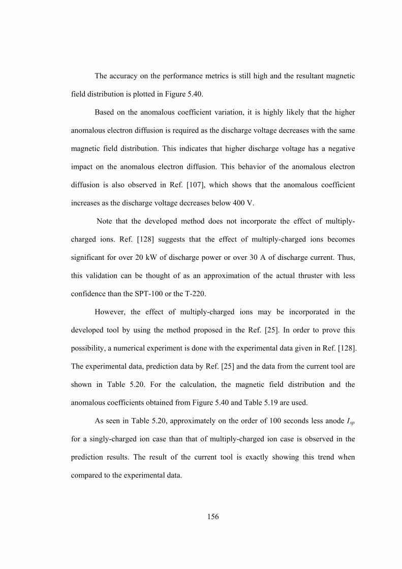
156
The accuracy on the performance metrics is still high and the resultant magnetic
field distribution is plotted in Figure 5.40.
Based on the anomalous coefficient variation, it is highly likely that the higher
anomalous electron diffusion is required as the discharge voltage decreases with the same
magnetic field distribution. This indicates that higher discharge voltage has a negative
impact on the anomalous electron diffusion. This behavior of the anomalous electron
diffusion is also observed in Ref. [107], which shows that the anomalous coefficient
increases as the discharge voltage decreases below 400 V.
Note that the developed method does not incorporate the effect of multiply-
charged ions. Ref. [128] suggests that the effect of multiply-charged ions becomes
significant for over 20 kW of discharge power or over 30 A of discharge current. Thus,
this validation can be thought of as an approximation of the actual thruster with less
confidence than the SPT-100 or the T-220.
However, the effect of multiply-charged ions may be incorporated in the
developed tool by using the method proposed in the Ref. [25]. In order to prove this
possibility, a numerical experiment is done with the experimental data given in Ref. [128].
The experimental data, prediction data by Ref. [25] and the data from the current tool are
shown in Table 5.20. For the calculation, the magnetic field distribution and the
anomalous coefficients obtained from Figure 5.40 and Table 5.19 are used.
As seen in Table 5.20, approximately on the order of 100 seconds less anode IRspR
for a singly-charged ion case than that of multiply-charged ion case is observed in the
prediction results. The result of the current tool is exactly showing this trend when
compared to the experimental data.
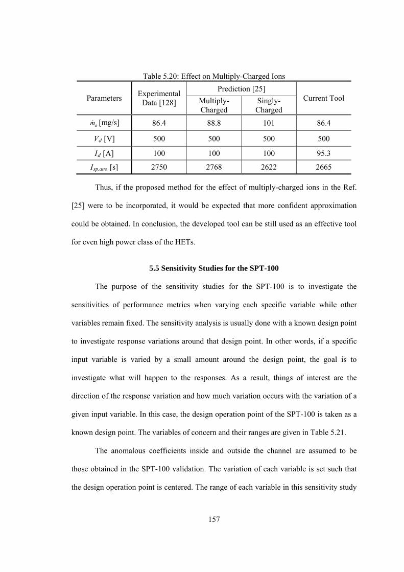
157
Table 5.20: Effect on Multiply-Charged Ions
Parameters Experimental
Data [128]
Prediction [25] Current Tool Multiply-
Charged Singly-Charged
am [mg/s] 86.4 88.8 101 86.4
VRdR [V] 500 500 500 500
IRdR [A] 100 100 100 95.3
IRsp,anoR [s] 2750 2768 2622 2665
Thus, if the proposed method for the effect of multiply-charged ions in the Ref.
[25] were to be incorporated, it would be expected that more confident approximation
could be obtained. In conclusion, the developed tool can be still used as an effective tool
for even high power class of the HETs.
5.5 Sensitivity Studies for the SPT-100
The purpose of the sensitivity studies for the SPT-100 is to investigate the
sensitivities of performance metrics when varying each specific variable while other
variables remain fixed. The sensitivity analysis is usually done with a known design point
to investigate response variations around that design point. In other words, if a specific
input variable is varied by a small amount around the design point, the goal is to
investigate what will happen to the responses. As a result, things of interest are the
direction of the response variation and how much variation occurs with the variation of a
given input variable. In this case, the design operation point of the SPT-100 is taken as a
known design point. The variables of concern and their ranges are given in Table 5.21.
The anomalous coefficients inside and outside the channel are assumed to be
those obtained in the SPT-100 validation. The variation of each variable is set such that
the design operation point is centered. The range of each variable in this sensitivity study
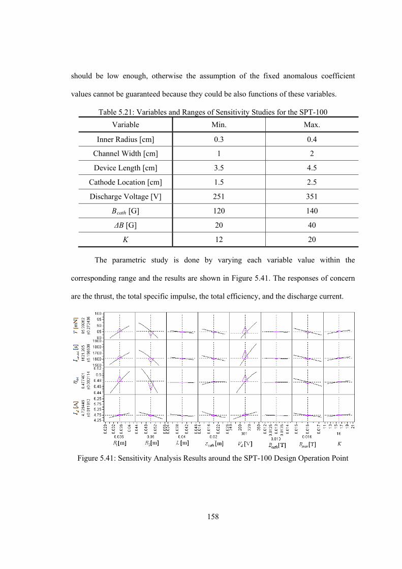
158
should be low enough, otherwise the assumption of the fixed anomalous coefficient
values cannot be guaranteed because they could be also functions of these variables.
Table 5.21: Variables and Ranges of Sensitivity Studies for the SPT-100
Variable Min. Max.
Inner Radius [cm] 0.3 0.4
Channel Width [cm] 1 2
Device Length [cm] 3.5 4.5
Cathode Location [cm] 1.5 2.5
Discharge Voltage [V] 251 351
BRcathR [G] 120 140
ΔB [G] 20 40
K 12 20
The parametric study is done by varying each variable value within the
corresponding range and the results are shown in Figure 5.41. The responses of concern
are the thrust, the total specific impulse, the total efficiency, and the discharge current.
Figure 5.41: Sensitivity Analysis Results around the SPT-100 Design Operation Point
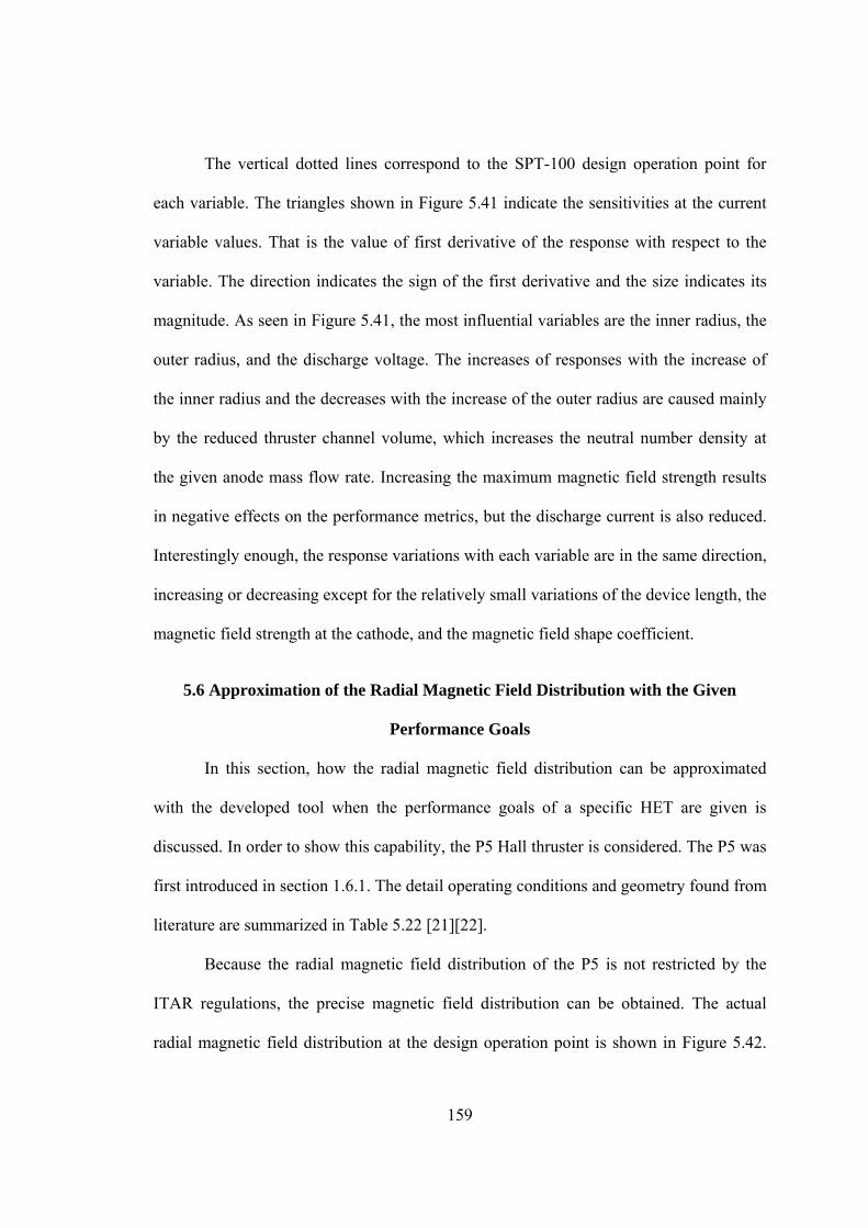
159
The vertical dotted lines correspond to the SPT-100 design operation point for
each variable. The triangles shown in Figure 5.41 indicate the sensitivities at the current
variable values. That is the value of first derivative of the response with respect to the
variable. The direction indicates the sign of the first derivative and the size indicates its
magnitude. As seen in Figure 5.41, the most influential variables are the inner radius, the
outer radius, and the discharge voltage. The increases of responses with the increase of
the inner radius and the decreases with the increase of the outer radius are caused mainly
by the reduced thruster channel volume, which increases the neutral number density at
the given anode mass flow rate. Increasing the maximum magnetic field strength results
in negative effects on the performance metrics, but the discharge current is also reduced.
Interestingly enough, the response variations with each variable are in the same direction,
increasing or decreasing except for the relatively small variations of the device length, the
magnetic field strength at the cathode, and the magnetic field shape coefficient.
5.6 Approximation of the Radial Magnetic Field Distribution with the Given
Performance Goals
In this section, how the radial magnetic field distribution can be approximated
with the developed tool when the performance goals of a specific HET are given is
discussed. In order to show this capability, the P5 Hall thruster is considered. The P5 was
first introduced in section 1.6.1. The detail operating conditions and geometry found from
literature are summarized in Table 5.22 [21][22].
Because the radial magnetic field distribution of the P5 is not restricted by the
ITAR regulations, the precise magnetic field distribution can be obtained. The actual
radial magnetic field distribution at the design operation point is shown in Figure 5.42.
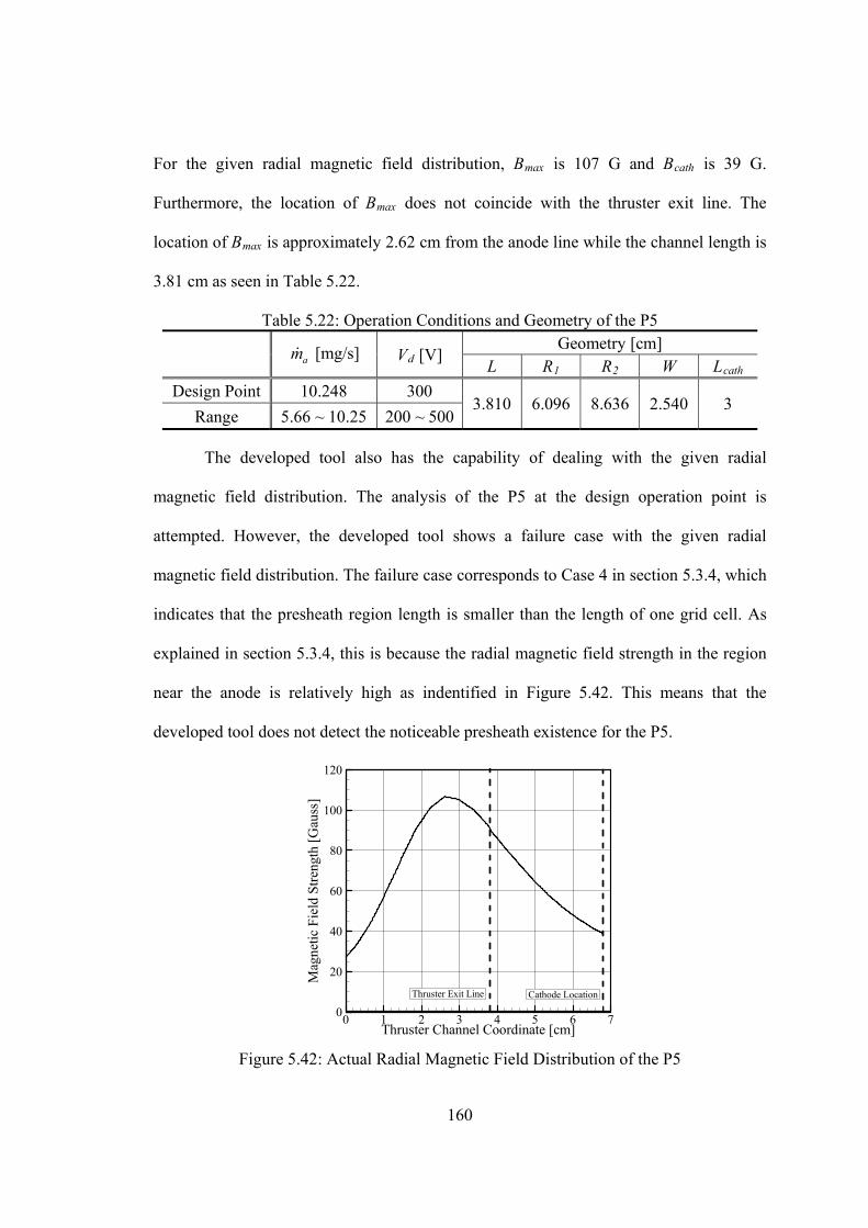
160
For the given radial magnetic field distribution, BRmaxR is 107 G and BRcathR is 39 G.
Furthermore, the location of BRmaxR does not coincide with the thruster exit line. The
location of BRmaxR is approximately 2.62 cm from the anode line while the channel length is
3.81 cm as seen in Table 5.22.
Table 5.22: Operation Conditions and Geometry of the P5
am [mg/s] VRdR [V] Geometry [cm]
L RR1 RR2 W LRcath
Design Point 10.248 300 3.810 6.096 8.636 2.540 3
Range 5.66 ~ 10.25 200 ~ 500
The developed tool also has the capability of dealing with the given radial
magnetic field distribution. The analysis of the P5 at the design operation point is
attempted. However, the developed tool shows a failure case with the given radial
magnetic field distribution. The failure case corresponds to Case 4 in section 5.3.4, which
indicates that the presheath region length is smaller than the length of one grid cell. As
explained in section 5.3.4, this is because the radial magnetic field strength in the region
near the anode is relatively high as indentified in Figure 5.42. This means that the
developed tool does not detect the noticeable presheath existence for the P5.
Thruster Channel Coordinate [cm]
Mag
netic
Fie
ldS
tren
gth
[Gau
ss]
0 1 2 3 4 5 6 70
20
40
60
80
100
120
Cathode LocationThruster Exit Line
Figure 5.42: Actual Radial Magnetic Field Distribution of the P5
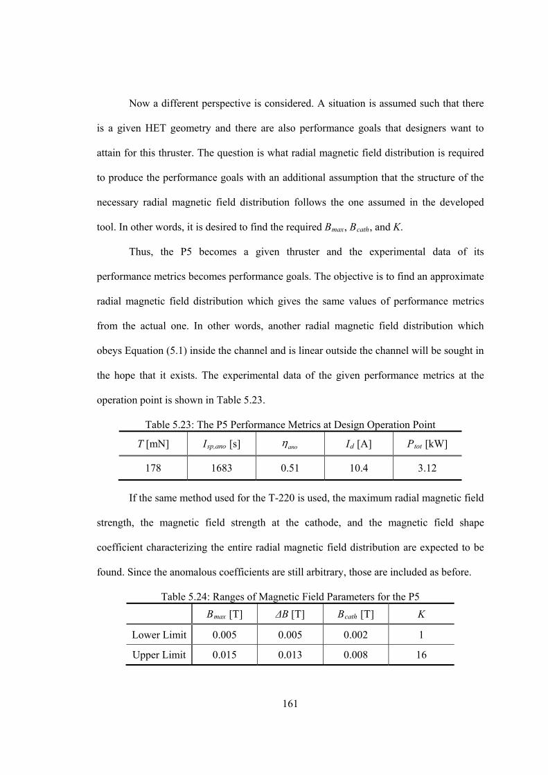
161
Now a different perspective is considered. A situation is assumed such that there
is a given HET geometry and there are also performance goals that designers want to
attain for this thruster. The question is what radial magnetic field distribution is required
to produce the performance goals with an additional assumption that the structure of the
necessary radial magnetic field distribution follows the one assumed in the developed
tool. In other words, it is desired to find the required BRmaxR, BRcathR, and K.
Thus, the P5 becomes a given thruster and the experimental data of its
performance metrics becomes performance goals. The objective is to find an approximate
radial magnetic field distribution which gives the same values of performance metrics
from the actual one. In other words, another radial magnetic field distribution which
obeys Equation (5.1) inside the channel and is linear outside the channel will be sought in
the hope that it exists. The experimental data of the given performance metrics at the
operation point is shown in Table 5.23.
Table 5.23: The P5 Performance Metrics at Design Operation Point
T [mN] IRsp,anoR [s] ano IRdR [A] PRtotR [kW]
178 1683 0.51 10.4 3.12
If the same method used for the T-220 is used, the maximum radial magnetic field
strength, the magnetic field strength at the cathode, and the magnetic field shape
coefficient characterizing the entire radial magnetic field distribution are expected to be
found. Since the anomalous coefficients are still arbitrary, those are included as before.
Table 5.24: Ranges of Magnetic Field Parameters for the P5
BRmaxR [T] ΔB [T] BRcathR [T] K
Lower Limit 0.005 0.005 0.002 1
Upper Limit 0.015 0.013 0.008 16
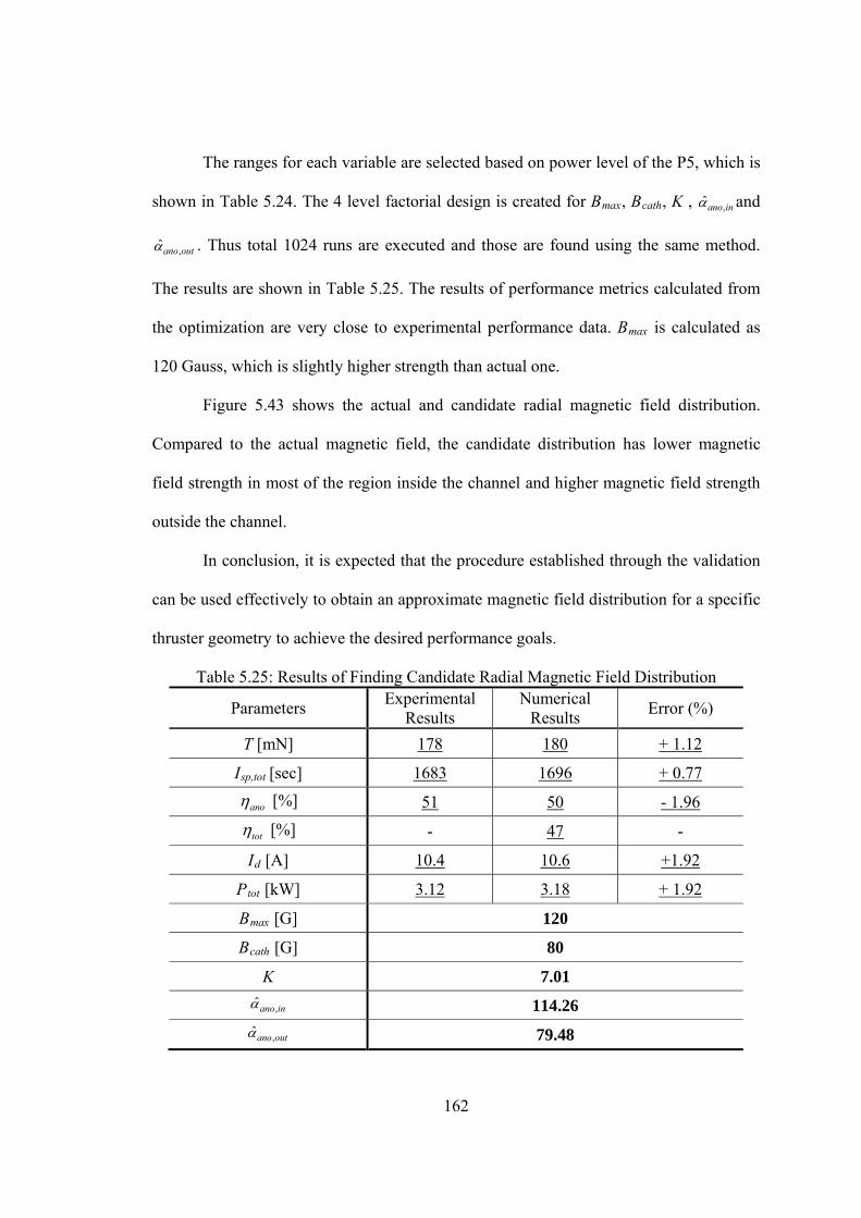
162
The ranges for each variable are selected based on power level of the P5, which is
shown in Table 5.24. The 4 level factorial design is created for BRmaxR, BRcathR, K , ,ˆano in and
,ˆano out . Thus total 1024 runs are executed and those are found using the same method.
The results are shown in Table 5.25. The results of performance metrics calculated from
the optimization are very close to experimental performance data. BRmaxR is calculated as
120 Gauss, which is slightly higher strength than actual one.
Figure 5.43 shows the actual and candidate radial magnetic field distribution.
Compared to the actual magnetic field, the candidate distribution has lower magnetic
field strength in most of the region inside the channel and higher magnetic field strength
outside the channel.
In conclusion, it is expected that the procedure established through the validation
can be used effectively to obtain an approximate magnetic field distribution for a specific
thruster geometry to achieve the desired performance goals.
Table 5.25: Results of Finding Candidate Radial Magnetic Field Distribution
Parameters Experimental
Results Numerical
Results Error (%)
T [mN] U178 U180 U+ 1.12
IRsp,tot R[sec] U1683 U1696 U+ 0.77
ano [%] U51 U50 U- 1.96
tot [%] - U47 -
IRdR [A] U10.4 U10.6 U+1.92
PRtotR [kW] U3.12 U3.18 U+ 1.92
BRmaxR [G] 120
BRcathR [G] 80
K 7.01
,ˆano in 114.26
,ˆano out 79.48
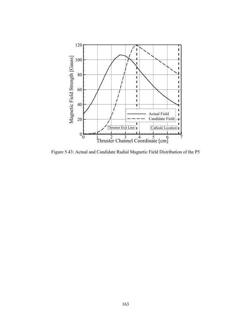
163
Thruster Channel Coordinate [cm]
Mag
netic
Fie
ldS
tren
gth
[Gau
ss]
0 1 2 3 4 5 6 70
20
40
60
80
100
120
Actual FieldCandidate Field
Cathode LocationThruster Exit Line
Figure 5.43: Actual and Candidate Radial Magnetic Field Distribution of the P5
164
CHAPTER 6
DESIGN SPACE EXPLORATION FOR HET
6.1 Need of Design Space Exploration
Based on validations with the HETs from 1 kW to 50 kW classes in the previous
chapter, it is expected that the developed tool can, in principle, be effectively used for the
design of a new HET in the conceptual design stage. It should be noted that the
implementation of the developed tool for design requires additional work as seen in the
validation process because the anomalous coefficients are arbitrary and there is currently
no way of calculating these coefficients a priori. In order to produce reliable designs, the
effects of these coefficients on the design should be incorporated in the design results.
The current method of incorporating the effects of the anomalous coefficients is
that they also be treated as design variables. In other words, the variation of the
anomalous coefficients also has impacts on the HET performance as other design
variables do. By doing this, design results are probabilistic rather than deterministic. This
is a reasonable strategy in the conceptual design stage because it can greatly reduce the
design space in spite of uncertainties in some variables.
The DSE can be accomplished by generating the data using numerical experiment,
which characterizes the entire design space. The advantages of the DSE are in general
that: 1) detail correlation information between input variables with respect to each
response can be obtained, 2) the feasible region, here the performance envelope, can be
165
identified, and 3) it could provide an environment for further investigations such as
optimization, sensitivity analysis, robust design, and probabilistic design.
6.2 Design Space Exploration for the HET
6.2.1 Selection of the Design Space
Defining the design space can be a quite difficult task due to the fact that: 1) the
ranges of variables determine the scope of the output response, 2) the output response
scope cannot be known before it is explored, 3) the output response scope should
effectively include the response goals, and 4) the DSE is a time-consuming process. Thus,
the selection of the design space tends to largely depend on accumulated experiences.
Because the DSE for the HET has not been done before, the situation becomes even
worse. However, the experiences gained from the validation work in the previous chapter,
which covers from 1 kW to 50 kW classes, are expected to aid in determining the HET
design space.
The current HET design is intended for near Earth missions. Figure 6.1 shows the
electric propulsion spacecraft operating near Earth [131]. Of all HETs on orbit, the SPT-
100 class is most common. These thrusters are primarily used for North South
Stationkeeping (NSSK) orbit control and momentum management. Their successful daily
operations for the geostationary communication satellites are well described in Ref. [132].
Recently, the PPSP
®P-1350-G HET was used for the SMART-1 mission, which is
the same power class as the SPT-100 [133]. Although it was used as a primary propulsion
system for this mission, it was originally developed for the implementation of the NSKK
of the GEO satellites constructed by Snecma.
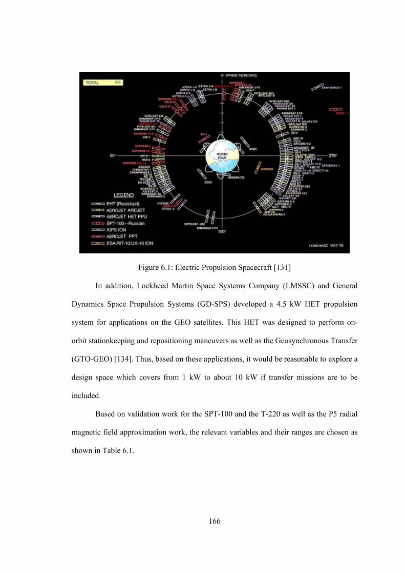
166
Figure 6.1: Electric Propulsion Spacecraft [131]
In addition, Lockheed Martin Space Systems Company (LMSSC) and General
Dynamics Space Propulsion Systems (GD-SPS) developed a 4.5 kW HET propulsion
system for applications on the GEO satellites. This HET was designed to perform on-
orbit stationkeeping and repositioning maneuvers as well as the Geosynchronous Transfer
(GTO-GEO) [134]. Thus, based on these applications, it would be reasonable to explore a
design space which covers from 1 kW to about 10 kW if transfer missions are to be
included.
Based on validation work for the SPT-100 and the T-220 as well as the P5 radial
magnetic field approximation work, the relevant variables and their ranges are chosen as
shown in Table 6.1.
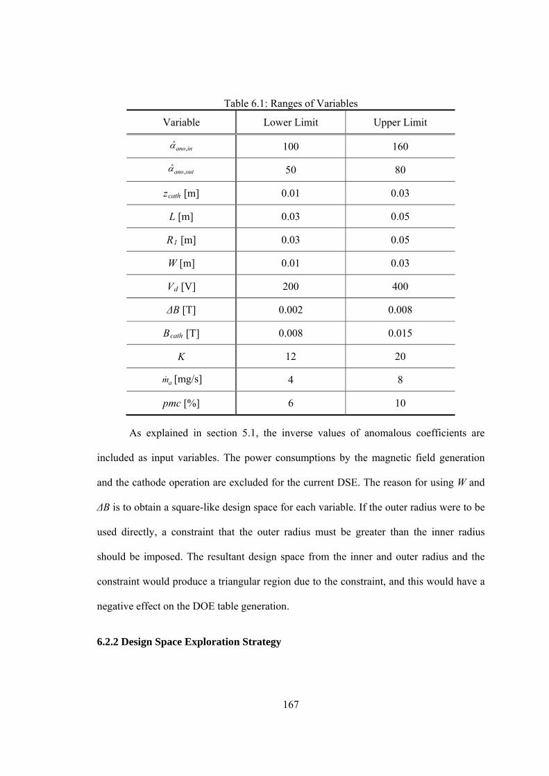
167
Table 6.1: Ranges of Variables
Variable Lower Limit Upper Limit
,ˆano in 100 160
,ˆano out 50 80
zRcathR [m] 0.01 0.03
L [m] 0.03 0.05
RR1R [m] 0.03 0.05
W [m] 0.01 0.03
VRdR [V] 200 400
ΔB [T] 0.002 0.008
BRcathR [T] 0.008 0.015
K 12 20
am [mg/s] 4 8
pmc [%] 6 10
As explained in section 5.1, the inverse values of anomalous coefficients are
included as input variables. The power consumptions by the magnetic field generation
and the cathode operation are excluded for the current DSE. The reason for using W and
ΔB is to obtain a square-like design space for each variable. If the outer radius were to be
used directly, a constraint that the outer radius must be greater than the inner radius
should be imposed. The resultant design space from the inner and outer radius and the
constraint would produce a triangular region due to the constraint, and this would have a
negative effect on the DOE table generation.
6.2.2 Design Space Exploration Strategy
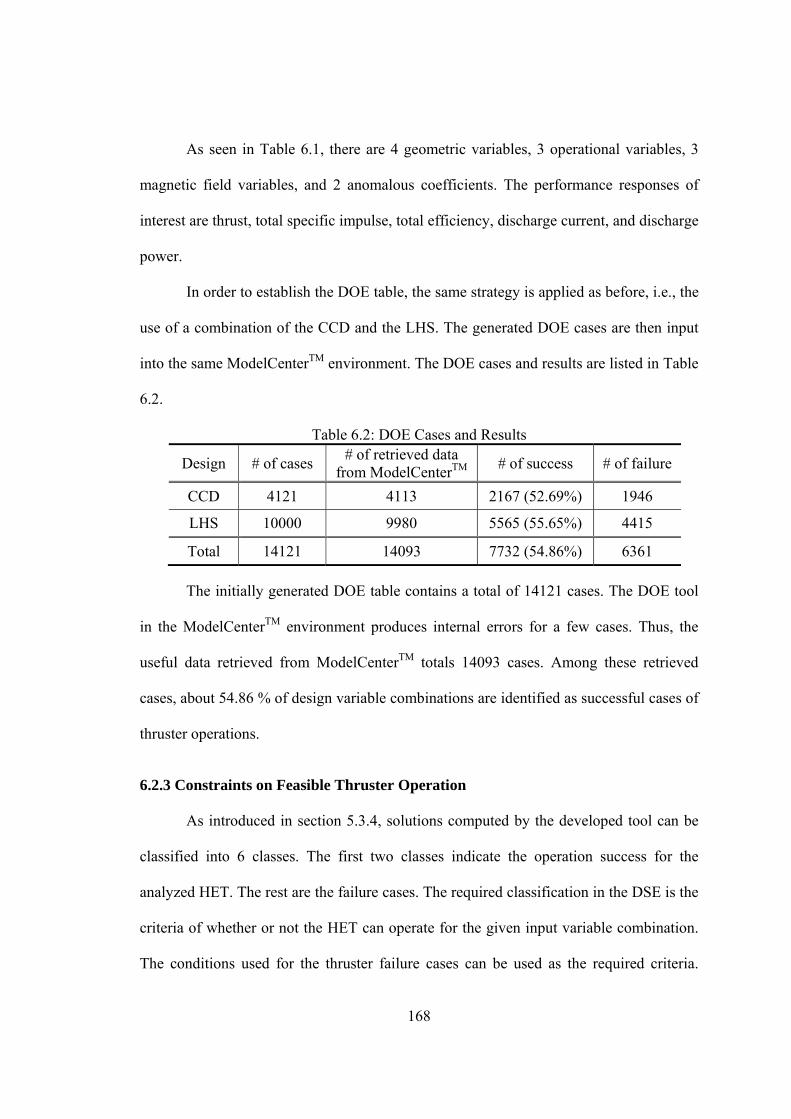
168
As seen in Table 6.1, there are 4 geometric variables, 3 operational variables, 3
magnetic field variables, and 2 anomalous coefficients. The performance responses of
interest are thrust, total specific impulse, total efficiency, discharge current, and discharge
power.
In order to establish the DOE table, the same strategy is applied as before, i.e., the
use of a combination of the CCD and the LHS. The generated DOE cases are then input
into the same ModelCenterP
TMP environment. The DOE cases and results are listed in Table
6.2.
Table 6.2: DOE Cases and Results
Design # of cases # of retrieved data
from ModelCenterP
TM # of success # of failure
CCD 4121 4113 2167 (52.69%) 1946
LHS 10000 9980 5565 (55.65%) 4415
Total 14121 14093 7732 (54.86%) 6361
The initially generated DOE table contains a total of 14121 cases. The DOE tool
in the ModelCenterP
TMP environment produces internal errors for a few cases. Thus, the
useful data retrieved from ModelCenterP
TMP totals 14093 cases. Among these retrieved
cases, about 54.86 % of design variable combinations are identified as successful cases of
thruster operations.
6.2.3 Constraints on Feasible Thruster Operation
As introduced in section 5.3.4, solutions computed by the developed tool can be
classified into 6 classes. The first two classes indicate the operation success for the
analyzed HET. The rest are the failure cases. The required classification in the DSE is the
criteria of whether or not the HET can operate for the given input variable combination.
The conditions used for the thruster failure cases can be used as the required criteria.
169
These conditions could be partially justified by the validation results in previous chapter
because the developed tool exhibits the thruster operation success at the experimental
operating points. Because the failure cases are determined by monitoring the internal
physical variables in the developed tool such as the plasma number density at the
matching point, the presheath region length, and the electron mean velocity at the cathode,
the constraints on the thruster operation success seem to come from a physically plausible
basis. For example, the constraint on the presheath region length for case 4 entails the
assumption that the noticeable presheath region is identified and accordingly, the ion
backflow region in the presheath exists. This assumption entails very low radial magnetic
field strength at the region near the anode. In the design perspective, this should not be a
problem because low magnetic field strength can be applied in a designed HET
accordingly.
Based on the discussion in section 5.3.4, the constraints can be quantitatively
expressed as Equation (6.1).
1 , ,
2
3 ,
4
| | 3
| 4
| 5
| 6
e m cal e m initial
m cal
e c cal
m cal
g n n corresponds to Case
g z dz corresponds to Case
g u corresponds to Case
g z L corresponds to Case
(6.1)
In Equation (6.1), all the variables are in non-dimensional units defined in
Appendix C. In constraint 1, the calculated plasma number density at the matching must
be greater than the initial guessed value. The initial guessed value is low and set to be 1e-
16 #/mP
3P. In constraint 2, dz is the length of one grid cell. If the presheath region length is
less than dz, it is considered that there exists no noticeable presheath and the presheath
region collapses in a very thin region near the anode. Thus, all constraints must be greater

170
than zero for the success of thruster operation. If any one of the constraints is violated,
the HET is considered to fail to operate for the given input variable combination.
In the hope that the constraints of gR1R ~ gR4R could reveal the performance envelope
for the given design space, the values of constraints are recorded during the DSE as well
as the required metrics.
6.2.4 Analysis of the DSE Results
The results of the DSE are retrieved from ModelCenterP
TMP and analyzed in the
JMPP
TMP environment. Table 6.3 shows the performance distribution and statistics for each
response. Thrust shows the highest standard deviation with variations from about 40 mN
to 200 mN.
The average of the total specific impulse is about 1850 sec, which varies from 950
sec to 2400 sec. The total efficiency has a short interquartile range and the maximum
value which can be obtained for the current design space is 0.633. The distributions of the
discharge current and the discharge power are similar. Their potential outliers are
distributed in the high value region and spreads in the wide range. The mean power is
2.65 kW for the current design space, however, the current design space includes the
power class from about 700 W to 10 kW, which is the intended power range.
Figure 6.2 shows the scatter plot for the responses, and shows all of the data
points and the relations between each pair of responses. Based on Figure 6.2, the
envelope of the feasible region can be approximately identified for each response.
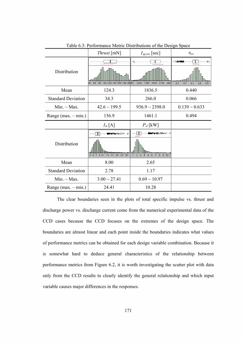
171
Table 6.3: Performance Metric Distributions of the Design Space
Thrust [mN] IRsp,totR [sec] tot
Distribution
Mean 124.3 1836.5 0.440
Standard Deviation 34.3 266.0 0.066
Min. ~ Max. 42.6 ~ 199.5 936.9 ~ 2398.0 0.139 ~ 0.633
Range (max. – min.) 156.9 1461.1 0.494
IRdR [A] PRdR [kW]
Distribution
Mean 8.00 2.65
Standard Deviation 2.78 1.17
Min. ~ Max. 3.00 ~ 27.41 0.69 ~ 10.97
Range (max. – min.) 24.41 10.28
The clear boundaries seen in the plots of total specific impulse vs. thrust and
discharge power vs. discharge current come from the numerical experimental data of the
CCD cases because the CCD focuses on the extremes of the design space. The
boundaries are almost linear and each point inside the boundaries indicates what values
of performance metrics can be obtained for each design variable combination. Because it
is somewhat hard to deduce general characteristics of the relationship between
performance metrics from Figure 6.2, it is worth investigating the scatter plot with data
only from the CCD results to clearly identify the general relationship and which input
variable causes major differences in the responses.
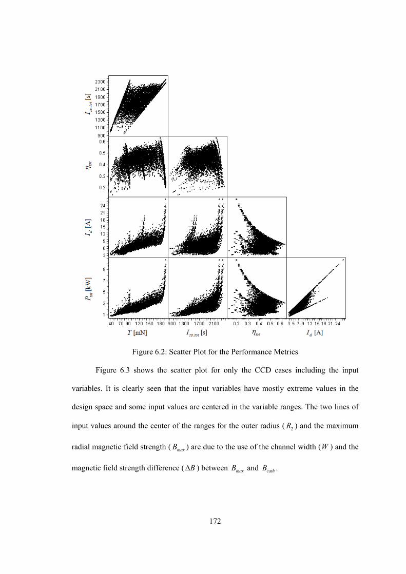
172
Figure 6.2: Scatter Plot for the Performance Metrics
Figure 6.3 shows the scatter plot for only the CCD cases including the input
variables. It is clearly seen that the input variables have mostly extreme values in the
design space and some input values are centered in the variable ranges. The two lines of
input values around the center of the ranges for the outer radius ( 2R ) and the maximum
radial magnetic field strength ( maxB ) are due to the use of the channel width (W ) and the
magnetic field strength difference ( B ) between maxB and cathB .
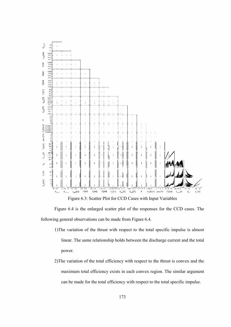
173
Figure 6.3: Scatter Plot for CCD Cases with Input Variables
Figure 6.4 is the enlarged scatter plot of the responses for the CCD cases. The
following general observations can be made from Figure 6.4.
1)The variation of the thrust with respect to the total specific impulse is almost
linear. The same relationship holds between the discharge current and the total
power.
2)The variation of the total efficiency with respect to the thrust is convex and the
maximum total efficiency exists in each convex region. The similar argument
can be made for the total efficiency with respect to the total specific impulse.
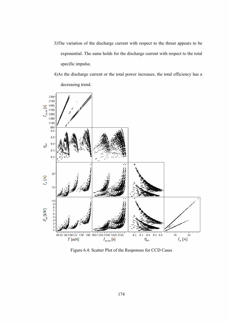
174
3)The variation of the discharge current with respect to the thrust appears to be
exponential. The same holds for the discharge current with respect to the total
specific impulse.
4)As the discharge current or the total power increases, the total efficiency has a
decreasing trend.
Figure 6.4: Scatter Plot of the Responses for CCD Cases
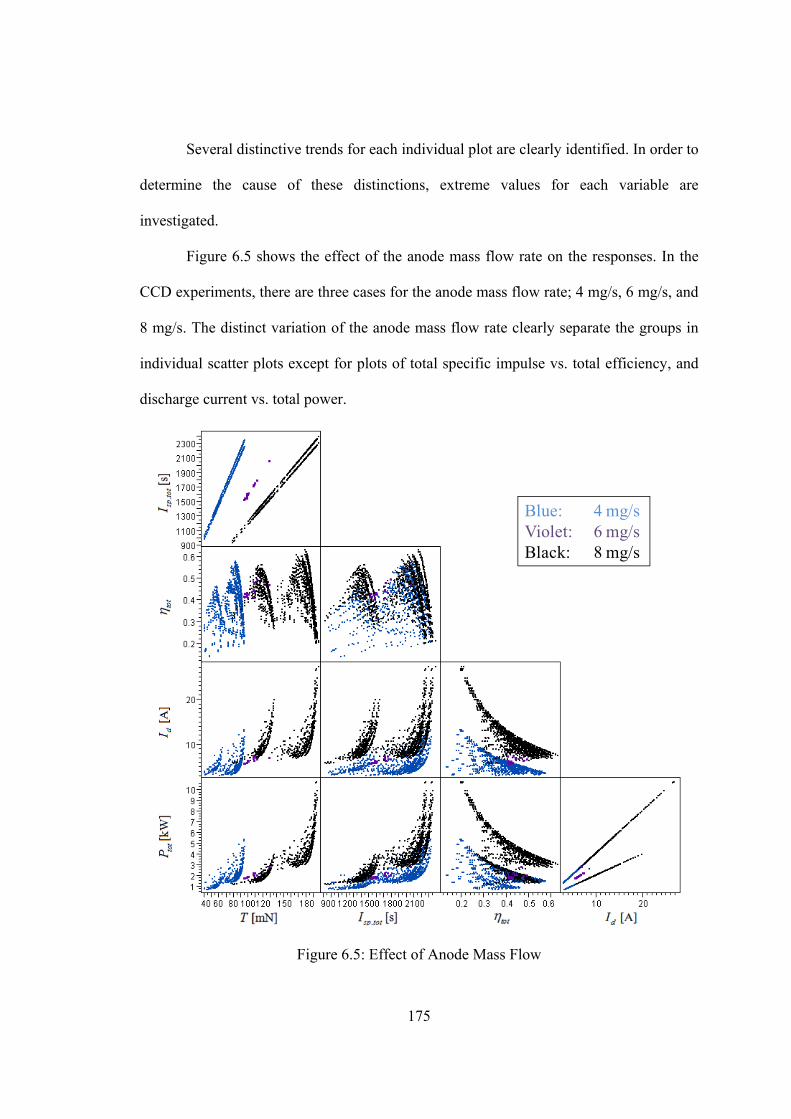
175
Several distinctive trends for each individual plot are clearly identified. In order to
determine the cause of these distinctions, extreme values for each variable are
investigated.
Figure 6.5 shows the effect of the anode mass flow rate on the responses. In the
CCD experiments, there are three cases for the anode mass flow rate; 4 mg/s, 6 mg/s, and
8 mg/s. The distinct variation of the anode mass flow rate clearly separate the groups in
individual scatter plots except for plots of total specific impulse vs. total efficiency, and
discharge current vs. total power.
Blue: 4 mg/sViolet: 6 mg/sBlack: 8 mg/s
Figure 6.5: Effect of Anode Mass Flow
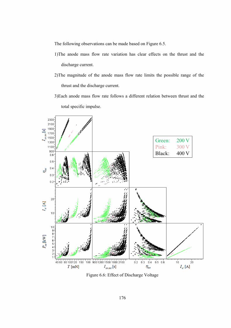
176
The following observations can be made based on Figure 6.5.
1)The anode mass flow rate variation has clear effects on the thrust and the
discharge current.
2)The magnitude of the anode mass flow rate limits the possible range of the
thrust and the discharge current.
3)Each anode mass flow rate follows a different relation between thrust and the
total specific impulse.
Green: 200 VPink: 300 VBlack: 400 V
Figure 6.6: Effect of Discharge Voltage

177
Figure 6.6 shows the effect of the discharge voltage on the responses. There are
three cases which are 200 V, 300 V, and 400 V. The distinctive regions are also identified
in plots of thrust vs. total efficiency, and total specific impulse vs. total efficiency. The
following observations can be made for the discharge voltage variations.
1)The discharge voltage variation has clear effects on the total specific impulse
and the total power.
2)The effect of the discharge voltage variation clearly limits the possible ranges of
total specific impulse, but weakly limits the total power range.
3)The lower discharge voltage can produce more thrust than higher discharge
voltage with the proper values of other parameters.
4)Each discharge voltage follows a different relationship between the discharge
current and the total power.
Although the discharge current and the total power are increased, it is interesting
to note that the combination of increased discharge voltage and increased anode mass
flow rate produces slightly higher maximum attainable total efficiency.
Figure 6.7 shows the effect of the outer radius of the channel on the responses.
There are three cases which are 4 cm, 6 cm, and 8 cm. There is no distinctive region
identified for the outer radius. However, the effect is given in each group of response. For
example, a small radius tends to produce a higher total efficiency, a lower discharge
current, and a lower total power in each group for the current design space.
There are not many noticeable effects identified for other input variable variations.
One is that a higher maximum magnetic field in the given range provides slightly
favorable total efficiency values for a given group.
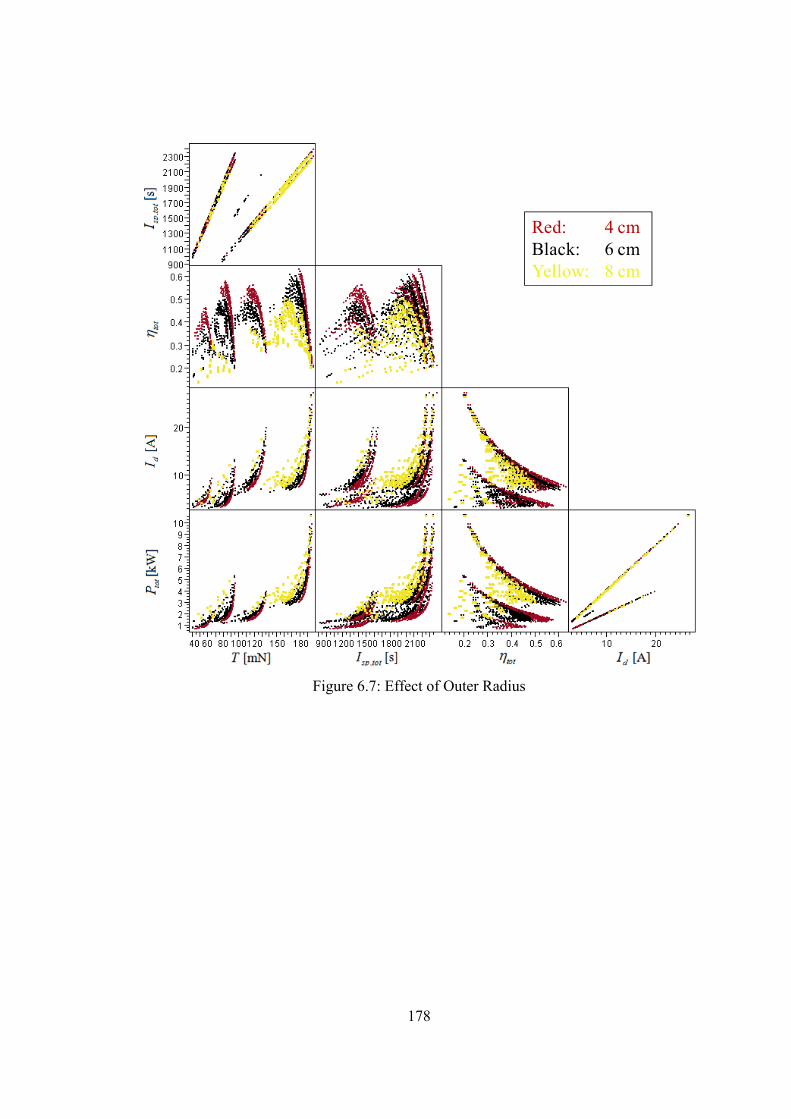
178
Red: 4 cmBlack: 6 cmYellow: 8 cm
Figure 6.7: Effect of Outer Radius
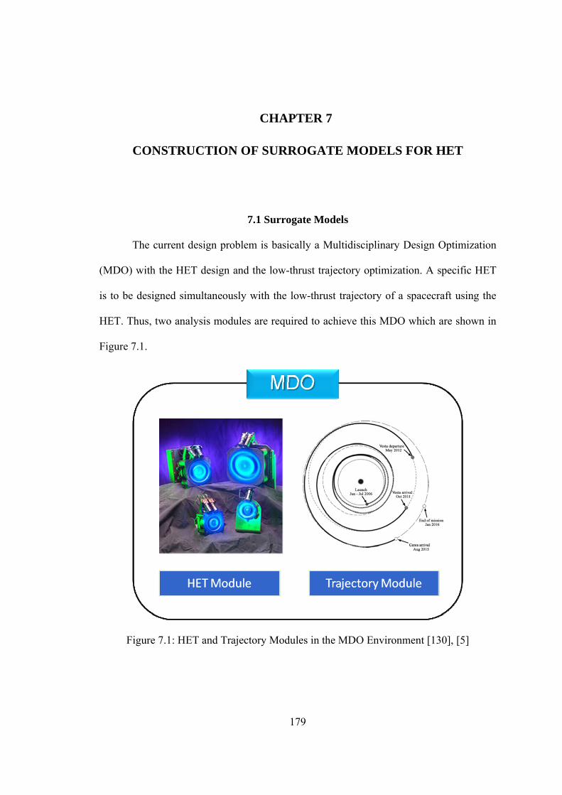
179
CHAPTER 7
CONSTRUCTION OF SURROGATE MODELS FOR HET
7.1 Surrogate Models
The current design problem is basically a Multidisciplinary Design Optimization
(MDO) with the HET design and the low-thrust trajectory optimization. A specific HET
is to be designed simultaneously with the low-thrust trajectory of a spacecraft using the
HET. Thus, two analysis modules are required to achieve this MDO which are shown in
Figure 7.1.
Figure 7.1: HET and Trajectory Modules in the MDO Environment [130], [5]
180
It is worth noting that the low-thrust trajectory optimization inherently uses
optimization algorithms to find the optimal trajectory, and the performance of the electric
thruster of interest is required to calculate the trajectory. The general goal of the
trajectory optimization is to minimize transfer time or maximize the final spacecraft mass.
The traditional low-thrust trajectory optimization has been done with a specifically
chosen simple electric thruster performance model as explained in section 1.7. As a result,
the thruster performance is fixed during the trajectory optimization except for the thrust.
On the other hand, the thruster performance needs to be varied in the current MDO,
which means that both the HET and the low-thrust trajectory are to be optimized
simultaneously to minimize transfer time or maximize the final spacecraft mass.
For this purpose, the HET performance analysis module and the trajectory
analysis module are combined under the global optimization environment and solved
simultaneously. Because it is expected that there are potentially thousands of function
calls for both modules during the optimization, it is highly desirable to construct proper
surrogate models for the HET. Although the developed tool (prior chapters) is
numerically efficient, more computationally efficient models, i.e., surrogate models for
each performance metric are demanded for the MDO purpose. Furthermore, the surrogate
models of the HET must produce performances for the given input variables close to
those from the actual developed tool. The acquired data from the DSE can be used to
construct the surrogate models of the HET by using a variety of statistical methods.
7.2 Surrogate Models for Performance Metrics using Response Surface
Methodology
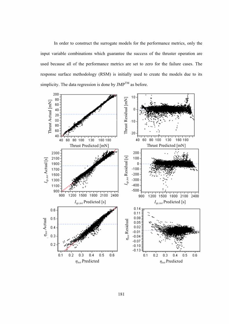
181
In order to construct the surrogate models for the performance metrics, only the
input variable combinations which guarantee the success of the thruster operation are
used because all of the performance metrics are set to zero for the failure cases. The
response surface methodology (RSM) is initially used to create the models due to its
simplicity. The data regression is done by JMPP
TMP as before.
Thr
ust A
ctua
l [m
N]
Thrust Predicted [mN]
Thr
ust
Res
idua
l [m
N]
Thrust Predicted [mN]
I sp,
totA
ctua
l [s]
Isp,tot Predicted [s]
Isp,tot Predicted [s]
I sp,
totR
esid
ual [
s]
η tot
Act
ual
ηtot Predicted
ηtot Predicted
η tot
Res
idua
l
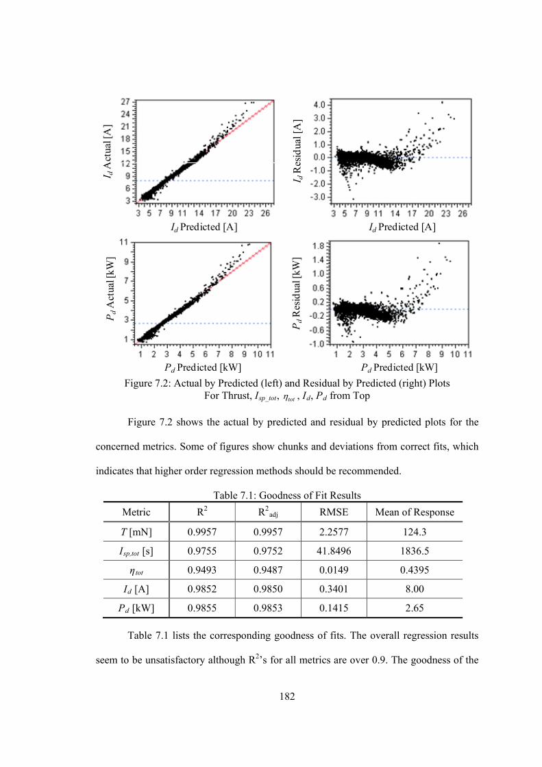
182
I dA
ctua
l [A
]
Id Predicted [A]
Id Predicted [A]
I dR
esid
ual [
A]
Pd
Act
ual [
kW]
Pd Predicted [kW]
Pd
Res
idua
l [kW
]
Pd Predicted [kW]
Figure 7.2: Actual by Predicted (left) and Residual by Predicted (right) Plots For Thrust, IRsp_totR, tot , IRdR, PRdR from Top
Figure 7.2 shows the actual by predicted and residual by predicted plots for the
concerned metrics. Some of figures show chunks and deviations from correct fits, which
indicates that higher order regression methods should be recommended.
Table 7.1: Goodness of Fit Results
Metric R P
2 RP
2PRadj RMSE Mean of Response
T [mN] 0.9957 0.9957 2.2577 124.3
IRsp,totR [s] 0.9755 0.9752 41.8496 1836.5
ηRtot 0.9493 0.9487 0.0149 0.4395
IRdR [A] 0.9852 0.9850 0.3401 8.00
PRdR [kW] 0.9855 0.9853 0.1415 2.65
Table 7.1 lists the corresponding goodness of fits. The overall regression results
seem to be unsatisfactory although RP
2P’s for all metrics are over 0.9. The goodness of the
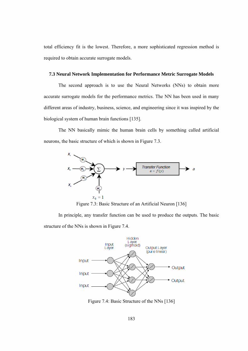
183
total efficiency fit is the lowest. Therefore, a more sophisticated regression method is
required to obtain accurate surrogate models.
7.3 Neural Network Implementation for Performance Metric Surrogate Models
The second approach is to use the Neural Networks (NNs) to obtain more
accurate surrogate models for the performance metrics. The NN has been used in many
different areas of industry, business, science, and engineering since it was inspired by the
biological system of human brain functions [135].
The NN basically mimic the human brain cells by something called artificial
neurons, the basic structure of which is shown in Figure 7.3.
Figure 7.3: Basic Structure of an Artificial Neuron [136]
In principle, any transfer function can be used to produce the outputs. The basic
structure of the NNs is shown in Figure 7.4.
Figure 7.4: Basic Structure of the NNs [136]

184
When the NNs are used for the regression purpose, several advantages can be
gained. They can handle highly nonlinear problems and the final regression equation is
given in a closed-form. The NNs can also handle continuous and discrete responses.
Although it is relatively more difficult to create and use than the RSM, the advantages are
fully appreciated once the corresponding NNs are created.
For the current purpose, the “BRAINN” program, which has been created in the
ASDL, is used. The purpose of this program is to provide the users with the automated
generation of neural network regressions [137]. The program is written in MATLABP
TMP
language and utilizes the Neural Net Toolbox in MATLABP
TMP. The snapshot of the
program is shown in Figure 7.5.
Figure 7.5: Snapshot of BRAINN Program [137]
In order to utilize the “BRAINN”, additional data sets are required such as
validation data and test data. The original data set is taken as a training data set used to
determine the Model Fit Error (MFE) of the resultant network. The validation data set is
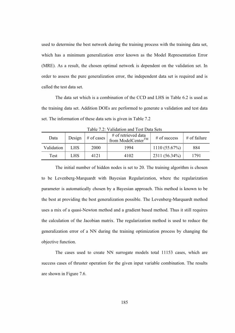
185
used to determine the best network during the training process with the training data set,
which has a minimum generalization error known as the Model Representation Error
(MRE). As a result, the chosen optimal network is dependent on the validation set. In
order to assess the pure generalization error, the independent data set is required and is
called the test data set.
The data set which is a combination of the CCD and LHS in Table 6.2 is used as
the training data set. Addition DOEs are performed to generate a validation and test data
set. The information of these data sets is given in Table 7.2
Table 7.2: Validation and Test Data Sets
Data Design # of cases# of retrieved data
from ModelCenter P
TM # of success # of failure
Validation LHS 2000 1994 1110 (55.67%) 884
Test LHS 4121 4102 2311 (56.34%) 1791
The initial number of hidden nodes is set to 20. The training algorithm is chosen
to be Levenberg-Marquardt with Bayesian Regularization, where the regularization
parameter is automatically chosen by a Bayesian approach. This method is known to be
the best at providing the best generalization possible. The Levenberg-Marquardt method
uses a mix of a quasi-Newton method and a gradient based method. Thus it still requires
the calculation of the Jacobian matrix. The regularization method is used to reduce the
generalization error of a NN during the training optimization process by changing the
objective function.
The cases used to create NN surrogate models total 11153 cases, which are
success cases of thruster operation for the given input variable combination. The results
are shown in Figure 7.6.
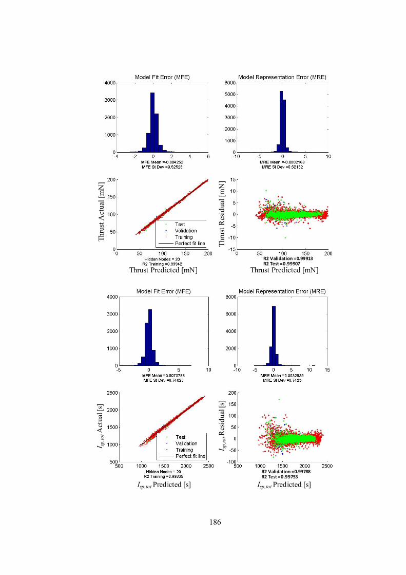
186
Thr
ust A
ctua
l [m
N]
Thrust Predicted [mN]
Thr
ust
Res
idua
l [m
N]
Thrust Predicted [mN]
R2 Validation =0.99913R2 Test =0.99907
I sp,
totA
ctua
l [s]
Isp,tot Predicted [s] Isp,tot Predicted [s]
I sp,
totR
esid
ual [
s]
R2 Validation =0.99788R2 Test =0.99753
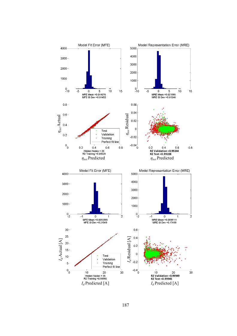
187
η tot
Act
ual
ηtot Predicted ηtot Predicted
η tot
Res
idua
l
R2 Validation =0.99244R2 Test =0.99228
I dA
ctua
l [A
]
Id Predicted [A] Id Predicted [A]
I dR
esid
ual [
A]
R2 Validation =0.99949R2 Test =0.99945
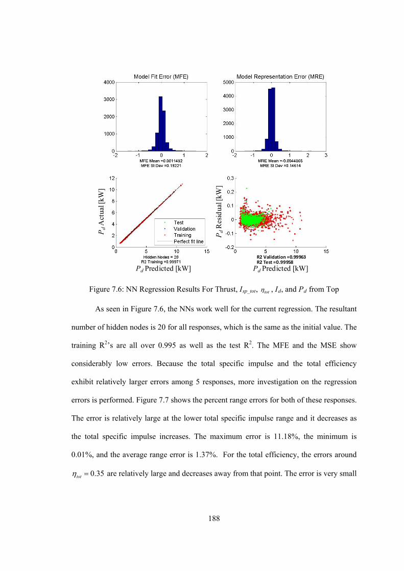
188
Pd
Act
ual [
kW]
Pd Predicted [kW]
Pd
Res
idua
l [kW
]
Pd Predicted [kW]
R2 Validation =0.99963R2 Test =0.99958
Figure 7.6: NN Regression Results For Thrust, IRsp_totR, tot , IRdR, and PRdR from Top
As seen in Figure 7.6, the NNs work well for the current regression. The resultant
number of hidden nodes is 20 for all responses, which is the same as the initial value. The
training RP
2P’s are all over 0.995 as well as the test RP
2P. The MFE and the MSE show
considerably low errors. Because the total specific impulse and the total efficiency
exhibit relatively larger errors among 5 responses, more investigation on the regression
errors is performed. Figure 7.7 shows the percent range errors for both of these responses.
The error is relatively large at the lower total specific impulse range and it decreases as
the total specific impulse increases. The maximum error is 11.18%, the minimum is
0.01%, and the average range error is 1.37%. For the total efficiency, the errors around
0.35tot are relatively large and decreases away from that point. The error is very small
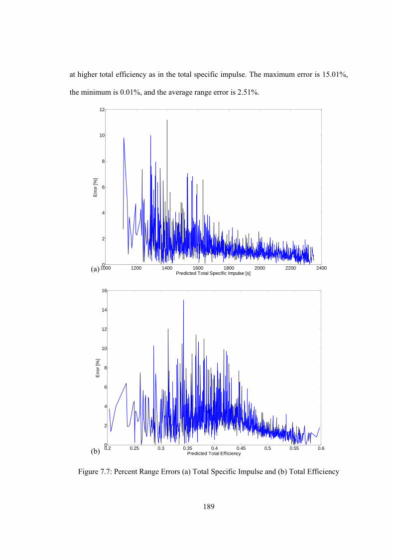
189
at higher total efficiency as in the total specific impulse. The maximum error is 15.01%,
the minimum is 0.01%, and the average range error is 2.51%.
1000 1200 1400 1600 1800 2000 2200 24000
2
4
6
8
10
12
Predicted Total Specific Impulse [s]
Err
or [%
]
0.2 0.25 0.3 0.35 0.4 0.45 0.5 0.55 0.60
2
4
6
8
10
12
14
16
Predicted Total Efficiency
Err
or [%
]
Figure 7.7: Percent Range Errors (a) Total Specific Impulse and (b) Total Efficiency
(a)
(b)
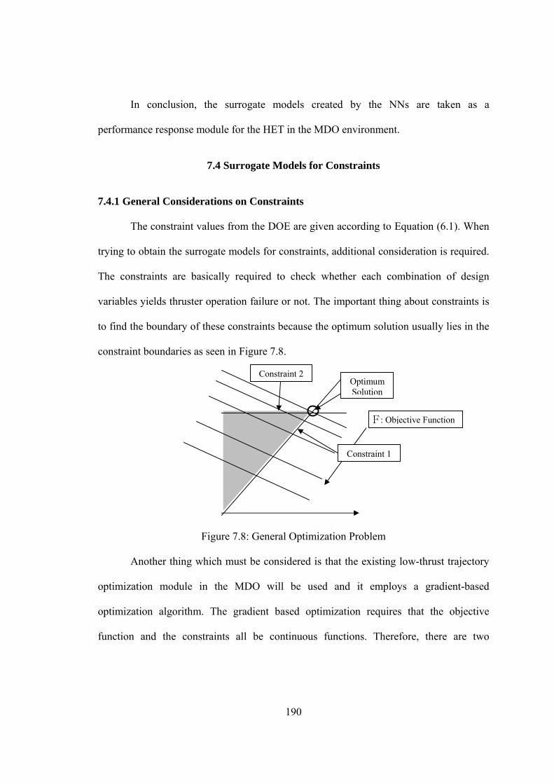
190
In conclusion, the surrogate models created by the NNs are taken as a
performance response module for the HET in the MDO environment.
7.4 Surrogate Models for Constraints
7.4.1 General Considerations on Constraints
The constraint values from the DOE are given according to Equation (6.1). When
trying to obtain the surrogate models for constraints, additional consideration is required.
The constraints are basically required to check whether each combination of design
variables yields thruster operation failure or not. The important thing about constraints is
to find the boundary of these constraints because the optimum solution usually lies in the
constraint boundaries as seen in Figure 7.8.
Figure 7.8: General Optimization Problem
Another thing which must be considered is that the existing low-thrust trajectory
optimization module in the MDO will be used and it employs a gradient-based
optimization algorithm. The gradient based optimization requires that the objective
function and the constraints all be continuous functions. Therefore, there are two
F
Optimum Solution
Constraint 1
Constraint 2
: Objective Function

191
objectives when building the surrogate models for the constraints: the constraints must
clearly identify the boundary, and the constraint functions must be continuous.
However, the constraint values of the thruster operation failure cases are obtained
as intermediate internal physical values because the developed tool cannot proceed to
produce the solutions as explained in section 5.3.4. In cases of the thruster operation
success, these constraint values, of course, are the converged values based on the plasma
number density at the matching point, the presheath region length, and the electron mean
velocity at the cathode. Therefore, if the regressions on these constraint values were to be
used and include the thruster operation failure cases, it is expected to be very poor.
Furthermore, it is also expected that the boundary separating the combinations into
operation success and failure is even harder to recognize.
Figure 7.9 shows the entire design space and the feasible region enclosed by the
boundary. The optimization in the MDO environment must be done in the feasible
thruster operation region.
Figure 7.9: Design Space and Feasible Region
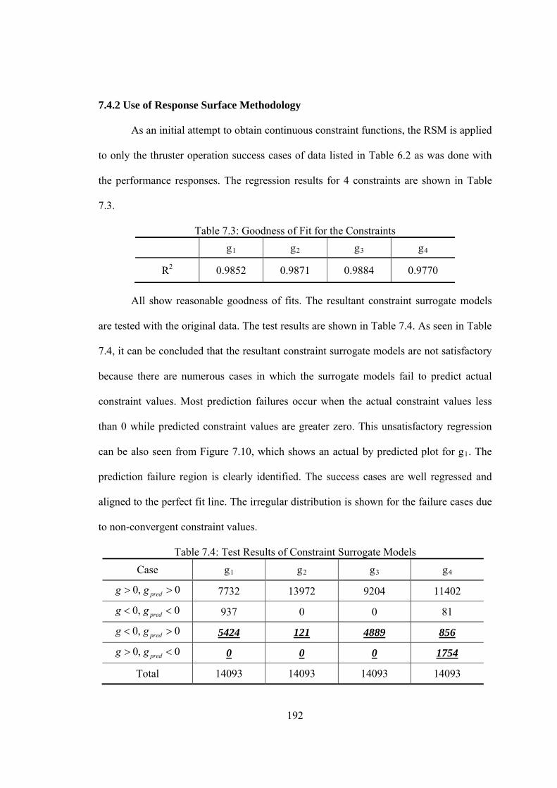
192
7.4.2 Use of Response Surface Methodology
As an initial attempt to obtain continuous constraint functions, the RSM is applied
to only the thruster operation success cases of data listed in Table 6.2 as was done with
the performance responses. The regression results for 4 constraints are shown in Table
7.3.
Table 7.3: Goodness of Fit for the Constraints
gR1 gR2 gR3 gR4
RP
2 0.9852 0.9871 0.9884 0.9770
All show reasonable goodness of fits. The resultant constraint surrogate models
are tested with the original data. The test results are shown in Table 7.4. As seen in Table
7.4, it can be concluded that the resultant constraint surrogate models are not satisfactory
because there are numerous cases in which the surrogate models fail to predict actual
constraint values. Most prediction failures occur when the actual constraint values less
than 0 while predicted constraint values are greater zero. This unsatisfactory regression
can be also seen from Figure 7.10, which shows an actual by predicted plot for gR1R. The
prediction failure region is clearly identified. The success cases are well regressed and
aligned to the perfect fit line. The irregular distribution is shown for the failure cases due
to non-convergent constraint values.
Table 7.4: Test Results of Constraint Surrogate Models
Case gR1 gR2 gR3 gR4
0, 0predg g 7732 13972 9204 11402
0, 0predg g 937 0 0 81
0, 0predg g U5424 U121 U4889 U856
0, 0predg g 0 0 0 U1754
Total 14093 14093 14093 14093
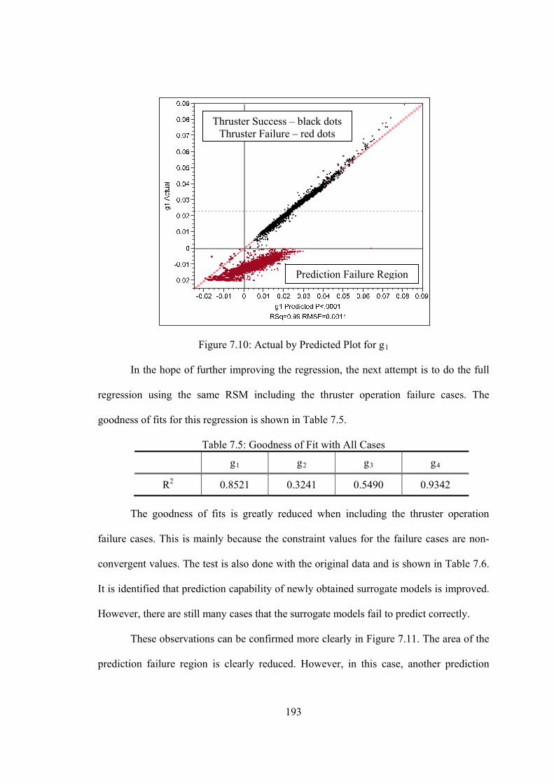
193
Figure 7.10: Actual by Predicted Plot for gR1
In the hope of further improving the regression, the next attempt is to do the full
regression using the same RSM including the thruster operation failure cases. The
goodness of fits for this regression is shown in Table 7.5.
Table 7.5: Goodness of Fit with All Cases
gR1 gR2 gR3 gR4
RP
2 0.8521 0.3241 0.5490 0.9342
The goodness of fits is greatly reduced when including the thruster operation
failure cases. This is mainly because the constraint values for the failure cases are non-
convergent values. The test is also done with the original data and is shown in Table 7.6.
It is identified that prediction capability of newly obtained surrogate models is improved.
However, there are still many cases that the surrogate models fail to predict correctly.
These observations can be confirmed more clearly in Figure 7.11. The area of the
prediction failure region is clearly reduced. However, in this case, another prediction
Prediction Failure Region
Thruster Success – black dots Thruster Failure – red dots
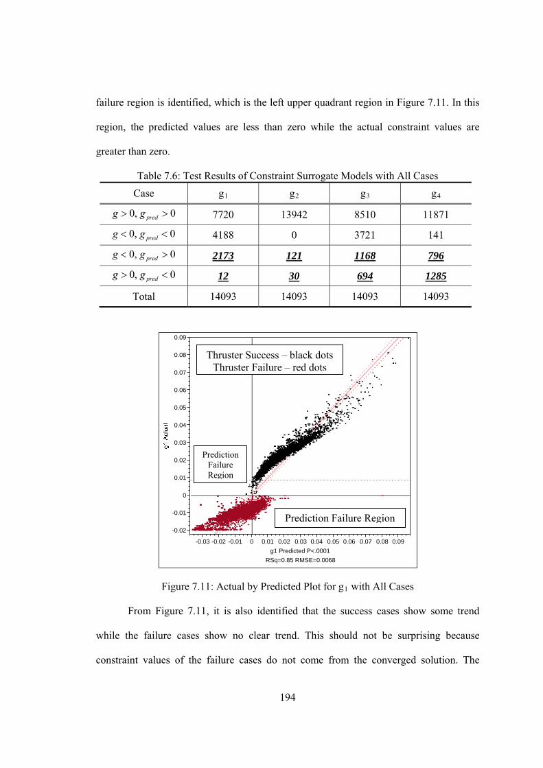
194
failure region is identified, which is the left upper quadrant region in Figure 7.11. In this
region, the predicted values are less than zero while the actual constraint values are
greater than zero.
Table 7.6: Test Results of Constraint Surrogate Models with All Cases
Case gR1 gR2 gR3 gR4
0, 0predg g 7720 13942 8510 11871
0, 0predg g 4188 0 3721 141
0, 0predg g U2173 U121 U1168 U796
0, 0predg g U12 U30 U694 U1285
Total 14093 14093 14093 14093
-0.02
-0.01
0
0.01
0.02
0.03
0.04
0.05
0.06
0.07
0.08
0.09
-0.03 -0.02 -0.01 0 0.01 0.02 0.03 0.04 0.05 0.06 0.07 0.08 0.09
g1 Predicted P<.0001
RSq=0.85 RMSE=0.0068
Figure 7.11: Actual by Predicted Plot for gR1R with All Cases
From Figure 7.11, it is also identified that the success cases show some trend
while the failure cases show no clear trend. This should not be surprising because
constraint values of the failure cases do not come from the converged solution. The
Thruster Success – black dots Thruster Failure – red dots
Prediction Failure Region
Prediction Failure Region
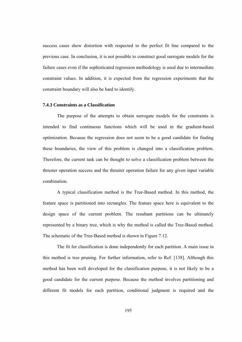
195
success cases show distortion with respected to the perfect fit line compared to the
previous case. In conclusion, it is not possible to construct good surrogate models for the
failure cases even if the sophisticated regression methodology is used due to intermediate
constraint values. In addition, it is expected from the regression experiments that the
constraint boundary will also be hard to identify.
7.4.3 Constraints as a Classification
The purpose of the attempts to obtain surrogate models for the constraints is
intended to find continuous functions which will be used in the gradient-based
optimization. Because the regression does not seem to be a good candidate for finding
these boundaries, the view of this problem is changed into a classification problem.
Therefore, the current task can be thought to solve a classification problem between the
thruster operation success and the thruster operation failure for any given input variable
combination.
A typical classification method is the Tree-Based method. In this method, the
feature space is partitioned into rectangles. The feature space here is equivalent to the
design space of the current problem. The resultant partitions can be ultimately
represented by a binary tree, which is why the method is called the Tree-Based method.
The schematic of the Tree-Based method is shown in Figure 7.12.
The fit for classification is done independently for each partition. A main issue in
this method is tree pruning. For further information, refer to Ref. [138]. Although this
method has been well developed for the classification purpose, it is not likely to be a
good candidate for the current purpose. Because the method involves partitioning and
different fit models for each partition, conditional judgment is required and the
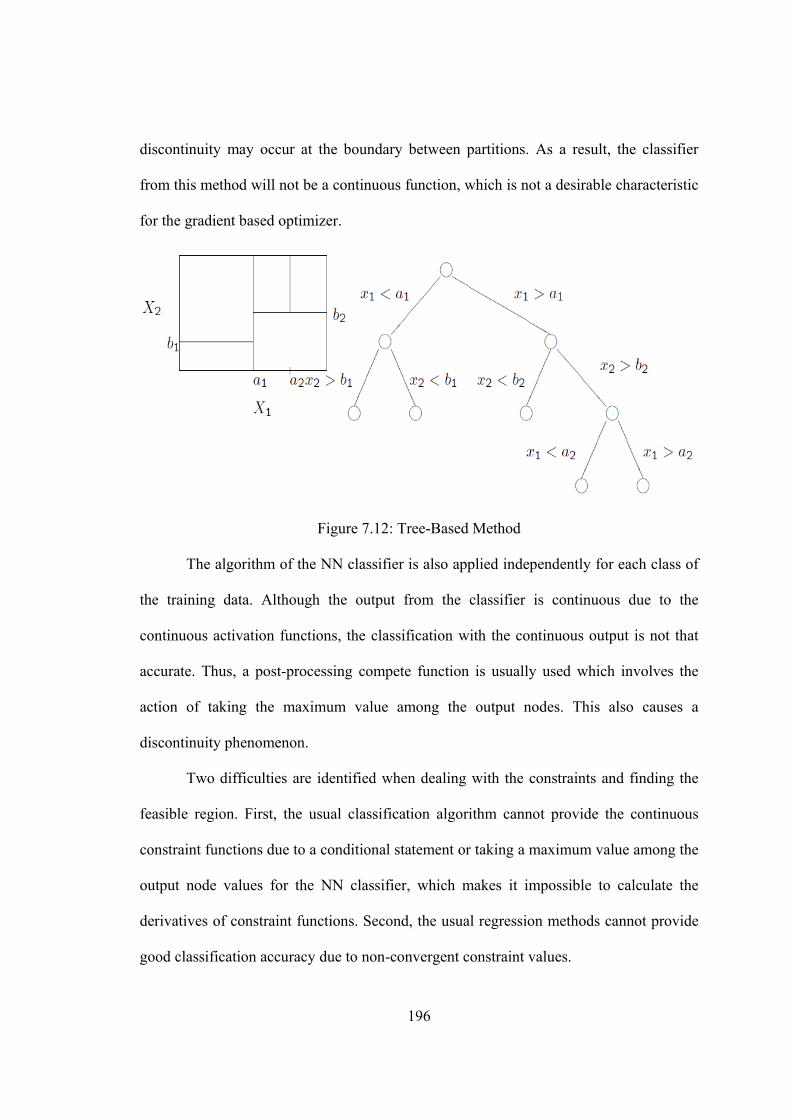
196
discontinuity may occur at the boundary between partitions. As a result, the classifier
from this method will not be a continuous function, which is not a desirable characteristic
for the gradient based optimizer.
Figure 7.12: Tree-Based Method
The algorithm of the NN classifier is also applied independently for each class of
the training data. Although the output from the classifier is continuous due to the
continuous activation functions, the classification with the continuous output is not that
accurate. Thus, a post-processing compete function is usually used which involves the
action of taking the maximum value among the output nodes. This also causes a
discontinuity phenomenon.
Two difficulties are identified when dealing with the constraints and finding the
feasible region. First, the usual classification algorithm cannot provide the continuous
constraint functions due to a conditional statement or taking a maximum value among the
output node values for the NN classifier, which makes it impossible to calculate the
derivatives of constraint functions. Second, the usual regression methods cannot provide
good classification accuracy due to non-convergent constraint values.
197
7.4.4 Support Vector Machine Classifier as a Constraint Function
The idea to resolve these difficulties is to use a Support Vector Machine (SVM)
classification algorithm. The SVM is a supervised learning method based on statistical
learning theory and its applications are classification and regression. The initial
development work is attributed mostly to Vapnik [139]. The SVM has been gaining
increasing attention and popularity due to many attractive features, and promising
empirical performance [140]. In addition to the basic statistical learning application, areas
of application are also increasing throughout science and engineering [141] - [142].
The classification problem in the SVM is to find an optimal hyperplane to
separate the data as shown in Figure 7.13. The hyperplane is a general term for separator
for any dimensional space. It will be a point for 1-D case, a line for 2-D case, or a plane
for 3-D case. The optimal hyperplane is a hyperplane which maximizes the margin. The
margin is the distance between the hyperplane and the nearest data point of each class.
Figure 7.13: Optimal Separating Hyperplane [140]
Thus, calculation of the SVM classifier involves an optimization problem to find
the optimal hyperplane. The simple binary classification and the corresponding classifier
are shown in the left of Figure 7.14. The nearest points from the optimal hyperplane are
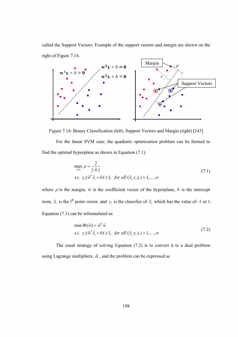
198
called the Support Vectors. Example of the support vectors and margin are shown on the
right of Figure 7.14.
Figure 7.14: Binary Classification (left), Support Vectors and Margin (right) [143]
For the linear SVM case, the quadratic optimization problem can be formed to
find the optimal hyperplane as shown in Equation (7.1).
,
,
2max
|| ||
. . ( ) 1, ( ), 1, ,
w b
Ti i i i
w
s t y w x b for all x y i n
(7.1)
where is the margin, w
is the coefficient vector of the hyperplane, b is the intercept
term, ix
is the iP
thP point vector, and iy is the classifier of ix
which has the value of -1 or 1.
Equation (7.1) can be reformulated as
,
min ( )
. . ( ) 1, ( ), 1, ,
T
Ti i i i
w w w
s t y w x b for all x y i n
(7.2)
The usual strategy of solving Equation (7.2) is to convert it to a dual problem
using Lagrange multipliers, , and the problem can be expressed as
Support Vectors
Margin
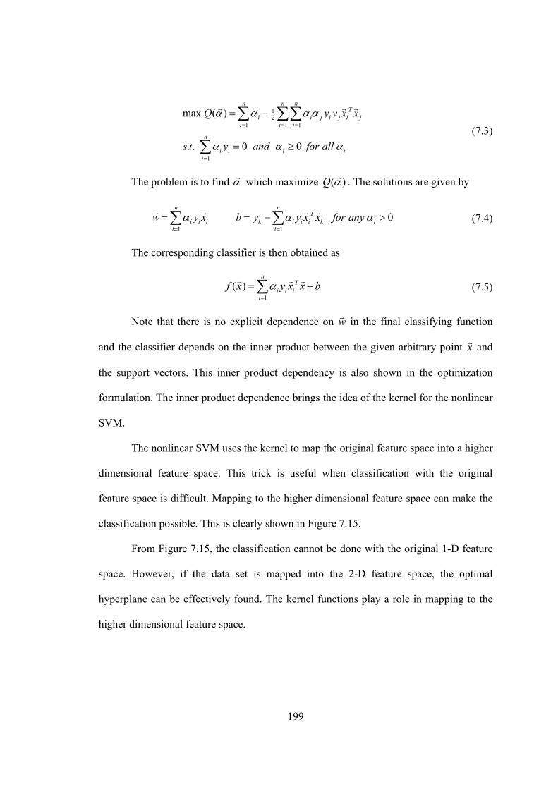
199
12
1 1 1
1
max ( )
. . 0 0
n n nT
i i j i j i ji i j
n
i i i ii
Q y y x x
s t y and for all
(7.3)
The problem is to find which maximize ( )Q . The solutions are given by
1 1
0n n
Ti i i k i i i k i
i i
w y x b y y x x for any
(7.4)
The corresponding classifier is then obtained as
1
( )n
Ti i i
i
f x y x x b
(7.5)
Note that there is no explicit dependence on w
in the final classifying function
and the classifier depends on the inner product between the given arbitrary point x
and
the support vectors. This inner product dependency is also shown in the optimization
formulation. The inner product dependence brings the idea of the kernel for the nonlinear
SVM.
The nonlinear SVM uses the kernel to map the original feature space into a higher
dimensional feature space. This trick is useful when classification with the original
feature space is difficult. Mapping to the higher dimensional feature space can make the
classification possible. This is clearly shown in Figure 7.15.
From Figure 7.15, the classification cannot be done with the original 1-D feature
space. However, if the data set is mapped into the 2-D feature space, the optimal
hyperplane can be effectively found. The kernel functions play a role in mapping to the
higher dimensional feature space.
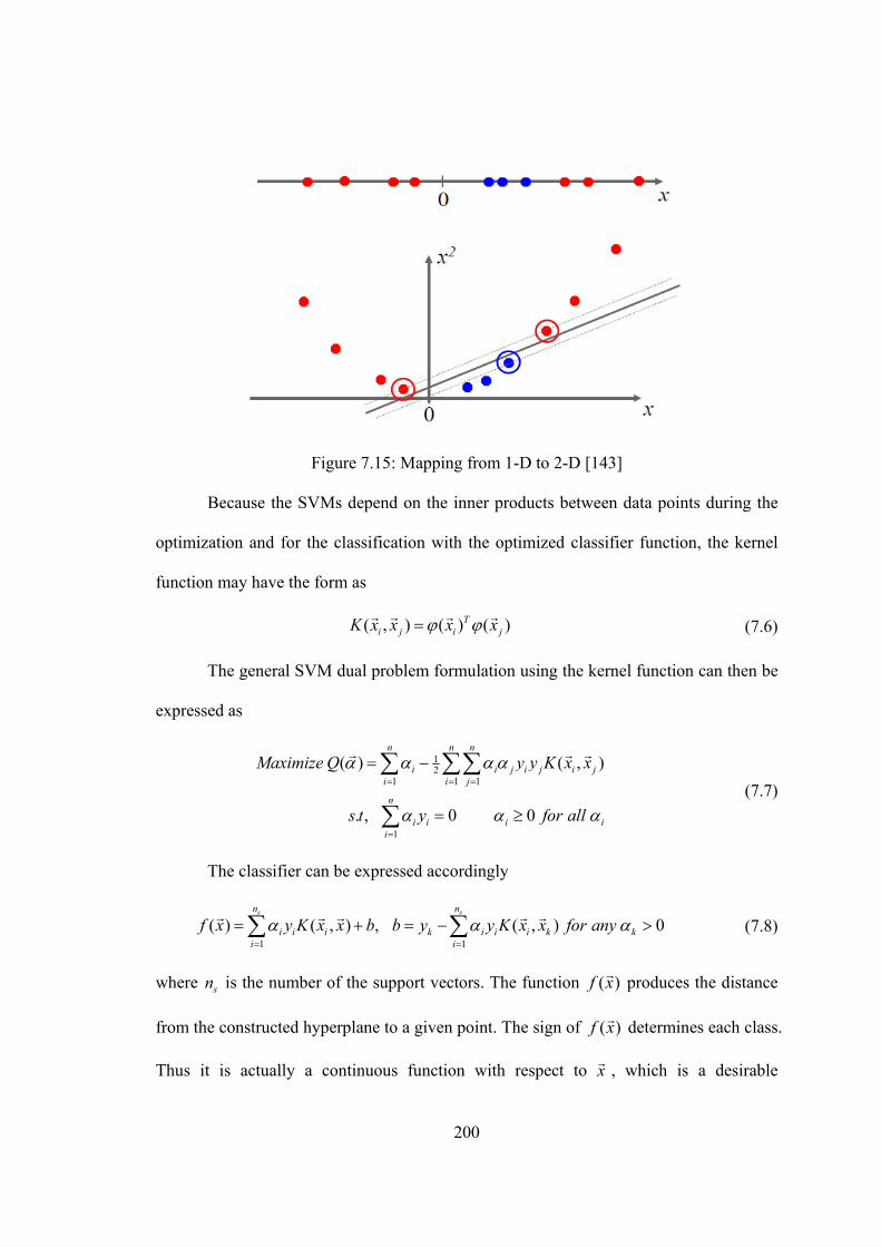
200
Figure 7.15: Mapping from 1-D to 2-D [143]
Because the SVMs depend on the inner products between data points during the
optimization and for the classification with the optimized classifier function, the kernel
function may have the form as
( , ) ( ) ( )Ti j i jK x x x x
(7.6)
The general SVM dual problem formulation using the kernel function can then be
expressed as
12
1 1 1
1
( ) ( , )
. , 0 0
n n n
i i j i j i ji i j
n
i i i ii
Maximize Q y y K x x
s t y for all
(7.7)
The classifier can be expressed accordingly
1 1
( ) ( , ) , ( , ) 0s sn n
i i i k i i i k ki i
f x y K x x b b y y K x x for any
(7.8)
where sn is the number of the support vectors. The function ( )f x
produces the distance
from the constructed hyperplane to a given point. The sign of ( )f x
determines each class.
Thus it is actually a continuous function with respect to x
, which is a desirable
201
characteristic for the current problem. Furthermore, because the SVMs are originally
intended for classification, it is expected that implementing the SVM to the current
problem will resolve the aforementioned two difficulties if the value of the function,
( )f x
is directly used without hard and soft classifications.
In order to implement the SVM, the SVM classifier in the Bioinformatics
ToolboxP
TMP of the MATLAB P
TMP is used. The SVM classifier in this software provides
three optimization methods to find the separating hyperplane, which are Quadratic
Programming (QP), Least-Squares (LS), and Sequential Minimal Optimization (SMO).
Because of high dimensionality and large data set of the current problem, the QP and the
LS cannot be used due to computer memory limitations. Thus, the SMO is used for
optimization in the SVM.
Before obtaining a desired classifying function, a proper kernel function should be
selected. The SVM classifier provides 5 kinds of the kernel functions such as linear,
quadratic, Gaussian Radial Basis Function, polynomial, and Multilayer Perceptron. Each
kernel functions are given as
2
2
2
|| ||
2
:
( , )
:
( , ) (1 )
:
( , ) (1 ) ,
:
( , ) ,i j
Ti j i j
Ti j i j
T pi j i j
x x
i j
Linear
K x x x x
Quadratic
K x x x x
Polynomial
K x x x x p polynomial order
Gaussian Radial Basis Function
K x x e scaling factor
Multilayer Perceptr
1 2 1 2
:
( , ) tanh( ), &Ti j i j
on
K x x p x x p p p scaling and bias parameters
(7.9)
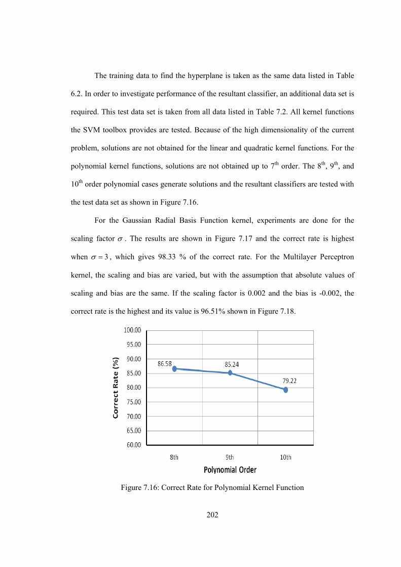
202
The training data to find the hyperplane is taken as the same data listed in Table
6.2. In order to investigate performance of the resultant classifier, an additional data set is
required. This test data set is taken from all data listed in Table 7.2. All kernel functions
the SVM toolbox provides are tested. Because of the high dimensionality of the current
problem, solutions are not obtained for the linear and quadratic kernel functions. For the
polynomial kernel functions, solutions are not obtained up to 7 P
thP order. The 8P
thP, 9 P
thP, and
10P
thP order polynomial cases generate solutions and the resultant classifiers are tested with
the test data set as shown in Figure 7.16.
For the Gaussian Radial Basis Function kernel, experiments are done for the
scaling factor . The results are shown in Figure 7.17 and the correct rate is highest
when 3 , which gives 98.33 % of the correct rate. For the Multilayer Perceptron
kernel, the scaling and bias are varied, but with the assumption that absolute values of
scaling and bias are the same. If the scaling factor is 0.002 and the bias is -0.002, the
correct rate is the highest and its value is 96.51% shown in Figure 7.18.
Figure 7.16: Correct Rate for Polynomial Kernel Function
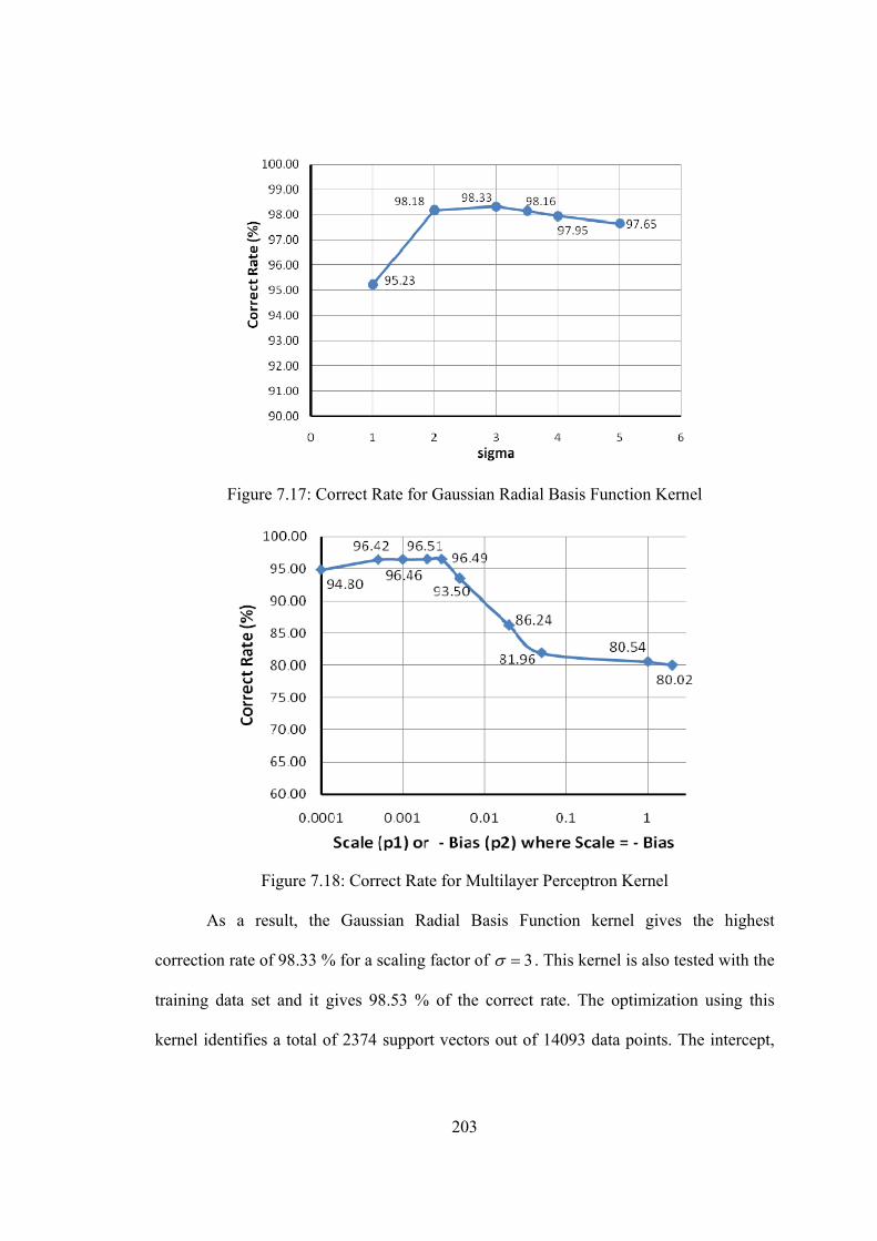
203
Figure 7.17: Correct Rate for Gaussian Radial Basis Function Kernel
Figure 7.18: Correct Rate for Multilayer Perceptron Kernel
As a result, the Gaussian Radial Basis Function kernel gives the highest
correction rate of 98.33 % for a scaling factor of 3 . This kernel is also tested with the
training data set and it gives 98.53 % of the correct rate. The optimization using this
kernel identifies a total of 2374 support vectors out of 14093 data points. The intercept,
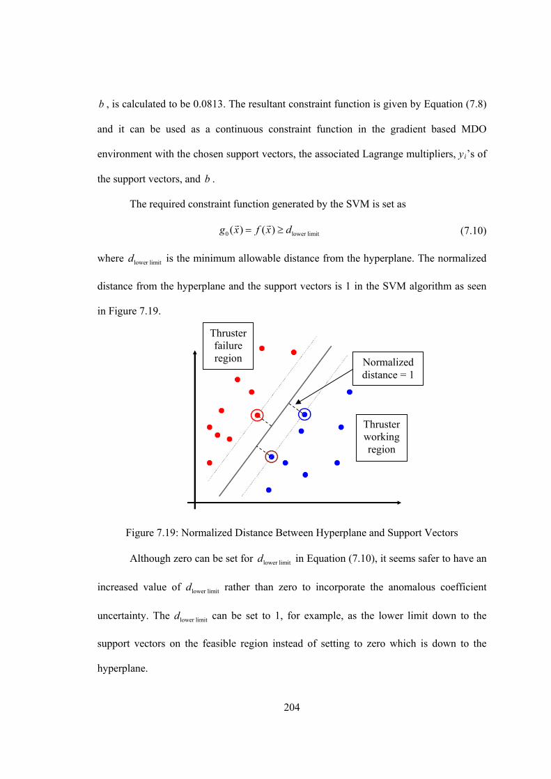
204
b , is calculated to be 0.0813. The resultant constraint function is given by Equation (7.8)
and it can be used as a continuous constraint function in the gradient based MDO
environment with the chosen support vectors, the associated Lagrange multipliers, yRiR’s of
the support vectors, and b .
The required constraint function generated by the SVM is set as
0 lower limit( ) ( )g x f x d
(7.10)
where lower limitd is the minimum allowable distance from the hyperplane. The normalized
distance from the hyperplane and the support vectors is 1 in the SVM algorithm as seen
in Figure 7.19.
Figure 7.19: Normalized Distance Between Hyperplane and Support Vectors
Although zero can be set for lower limitd in Equation (7.10), it seems safer to have an
increased value of lower limitd rather than zero to incorporate the anomalous coefficient
uncertainty. The lower limitd can be set to 1, for example, as the lower limit down to the
support vectors on the feasible region instead of setting to zero which is down to the
hyperplane.
Thruster working region
Thruster failure region Normalized
distance = 1

205
Now that the constraint function by the SVM is constructed, other constraint
functions generated by the NNs using only thruster operation success cases are no longer
needed. However, it would be useful to check the behavior of those constraint functions
in the MDO environment in order to compare them with the performance of the SVM
constraint function. All these constraints must be greater than or equal to zero to indicate
the feasible region.
206
CHAPTER 8
SIMULTANEOUS DESIGN OPTIMIZATION FOR AN ELECTRIC
ORBIT RAISING MISSION BY COLLABORATION WORK
8.0 Acknowledgement
It is acknowledged that this chapter is written in part by the efforts of
collaborators.
8.1 Mission Selection
The missions with SEP can be applied to such cases where a large acceleration is
not required and additional increased time of flight is not a significant factor [144].
Furthermore, as seen in Figure 1.1, SEP increases the possibility of achieving the high
V missions to which chemical propulsion is not applicable.
However, if a new HET is considered and designed, near-Earth missions should
be the focus because it is not expected that a new HET would be developed for a single
mission such as the Discovery class missions nor solar system explorations, or deep space
missions due to the large cost of new HET development. The near-Earth missions have
benefits in that there is still a high demand for communications satellites worldwide and
other near-Earth applications. If the advantages of SEP are fully appreciated with these
missions, more performance enhancement and cost-effective satellite operations can be
realized.

207
GEO satellites are now commonly using SEP for stationkeeping purposes. In
order to obtain greater mass transportation or extension of satellite lifetime while
reducing the launch cost, missions including near-Earth transfers using SEP should be
considered for future applications. Especially for the GEO satellites, combinations of
transfers and stationkeeping could produce considerable benefits from a systems
perspective compared to the present bi-propellant systems for an apogee insertion and
stationkeeping scenario, which requires about half of the total mass of the GEO satellites
for the propellant in the GTO [145]. Thus, there is a high possibility of increased use of
SEP for near-Earth missions and it is expected to increase in the near future.
However, due to long time of transfer with SEP, there are risks involving transfers
starting from the LEO such as radiation exposure in the Van Allen Radiation Belts and
collision with Earth-orbiting debris. Therefore, the mission considered here is the Orbit
Raising Mission (ORM). Generally speaking, the ORM refers to transportation from a
transfer orbit to the GEO regardless of the type of propulsion system. The ORM using the
electric thruster is termed as Electric Orbit Raising (EOR). The transfer mission from the
GTO to the GEO using the EOR has been researched with top-level analysis [146] and
found in some low-thruster trajectory optimization papers [147] - [149]. This transfer
mission still needs a transfer time on the order of 150 days and the number of revolutions
on the order of 200. In addition, a large part of the transfer trajectory is still exposed to a
high concentration of radiation. These drawbacks prevent the EOR from being part of
commercial applications.
In the low-thrust trajectory optimization perspective, problems with such a large
number of revolutions are difficult because the problems are often ill-posed and
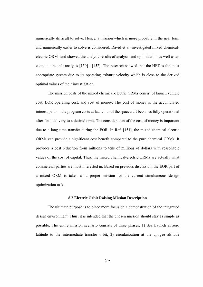
208
numerically difficult to solve. Hence, a mission which is more probable in the near term
and numerically easier to solve is considered. David et al. investigated mixed chemical-
electric ORMs and showed the analytic results of analysis and optimization as well as an
economic benefit analysis [150] - [152]. The research showed that the HET is the most
appropriate system due to its operating exhaust velocity which is close to the derived
optimal values of their investigation.
The mission costs of the mixed chemical-electric ORMs consist of launch vehicle
cost, EOR operating cost, and cost of money. The cost of money is the accumulated
interest paid on the program costs at launch until the spacecraft becomes fully operational
after final delivery to a desired orbit. The consideration of the cost of money is important
due to a long time transfer during the EOR. In Ref. [151], the mixed chemical-electric
ORMs can provide a significant cost benefit compared to the pure chemical ORMs. It
provides a cost reduction from millions to tens of millions of dollars with reasonable
values of the cost of capital. Thus, the mixed chemical-electric ORMs are actually what
commercial parties are most interested in. Based on previous discussion, the EOR part of
a mixed ORM is taken as a proper mission for the current simultaneous design
optimization task.
8.2 Electric Orbit Raising Mission Description
The ultimate purpose is to place more focus on a demonstration of the integrated
design environment. Thus, it is intended that the chosen mission should stay as simple as
possible. The entire mission scenario consists of three phases; 1) Sea Launch at zero
latitude to the intermediate transfer orbit, 2) circularization at the apogee altitude
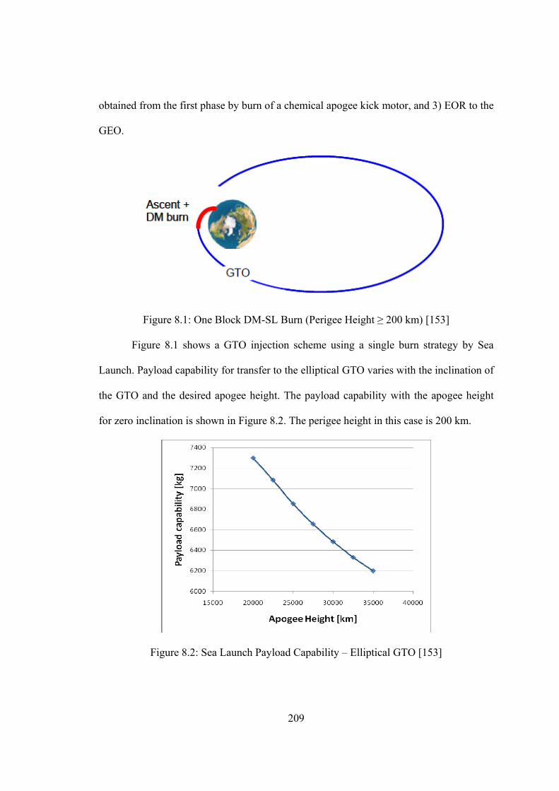
209
obtained from the first phase by burn of a chemical apogee kick motor, and 3) EOR to the
GEO.
Figure 8.1: One Block DM-SL Burn (Perigee Height ≥ 200 km) [153]
Figure 8.1 shows a GTO injection scheme using a single burn strategy by Sea
Launch. Payload capability for transfer to the elliptical GTO varies with the inclination of
the GTO and the desired apogee height. The payload capability with the apogee height
for zero inclination is shown in Figure 8.2. The perigee height in this case is 200 km.
Figure 8.2: Sea Launch Payload Capability – Elliptical GTO [153]
210
For the current problem, the apogee radius of the intermediate transfer orbit is
chosen to be 33000 km. The reason of choosing this radius is that the long time transfer
by the EOR can be started approximately at the outer edge of the Van Allen Radiation
Outer Belt, which minimizes the radiation exposure during the EOR. Then, it is further
assumed that the apogee kick motor, using a bipropellant chemical engine, is used to
circularize the orbit. In order to obtain full advantages of the EOR and minimize the
propellant for the bipropellant chemical system, the perigee is raised to the apogee radius
so that the circle-to-circle EOR can maximize the capability of SEP while minimizing the
radiation exposure. Finally, the EOR delivers the spacecraft to the final GEO.
The initial and final orbits of the EOR part are given in Table 8.1.
Table 8.1: Initial and Final Orbits of EOR
a (km) e i (deg) (deg) (deg) (deg)
Initial 33000 0 0 0 0 0
Final 42164 0 0 0 0 free
The spacecraft mass at t=0 is assumed to be 700 kg, which is well within the Sea
Launch payload capability. It is also assumed that the spacecraft is equipped with two
HETs. The objective is a minimum-fuel transfer. In order to make the trajectory
optimization easier to solve, it is decided that the time of flight is fixed. The time of flight
selected corresponds to the minimum time to accomplish the transfer using two SPT-100
engines, and is equal to 20.034 days. Based on this time of flight, the number of
revolutions would be approximately 1224 . There are two main reasons for this choice: 1)
in practice, it is best to minimize the time of flight to reduce the hazardous effects in the
radiation belt during the transfer, and 2) using the physics-based engine model does not
allow to switch off the engine during the transfer as will be explained in the next section.
211
8.3 Simultaneous Design Optimization Environment
The overall performance of a spacecraft is a function of both the spacecraft
trajectory and the engine design. Further, the engine design will impact the spacecraft
trajectory and vice versa. However, as explained before, the impact of simultaneously
considering both trajectory and engine design variables has not been previously
considered. In fact, the EP design problem is often carried out prior to the low-thrust
trajectory optimization problem. Therefore, it can be seen that this limitation might result
in a sub-optimal configuration. To improve results during the preliminary design, an ‘all-
at-a-time’ approach is adopted where engine and trajectory problems are optimized
together to obtain a solution. Therefore, an efficiently coupled MDO scheme is required
to account for the optimization of these two very different disciplines.
Current MDO approaches often involve a multistep sequential optimization
procedure. In the current context, this method would consist of a trajectory optimization
cycle (inner loop) and an engine design cycle (outer loop). The inner loop uses the data of
the outer loop to determine the engine system parameters yielding the optimum
performance as long as the departure from the preset design (outer loop) remains small.
However, this approach is not efficient for the current problem. Since such a strategy
requires many inner loop optimizations given by the number of outer loop iterations, it
would be inefficient. Low-thrust trajectory problems are computationally intensive and it
is therefore preferable to perform only one optimization per problem.
In this thesis, this issue can be avoided by transforming the MDO problem into a
single trajectory problem having both a static and a dynamic aspect. The dynamic aspect
involves all the variables that can be varied over time on the trajectory. The static aspect
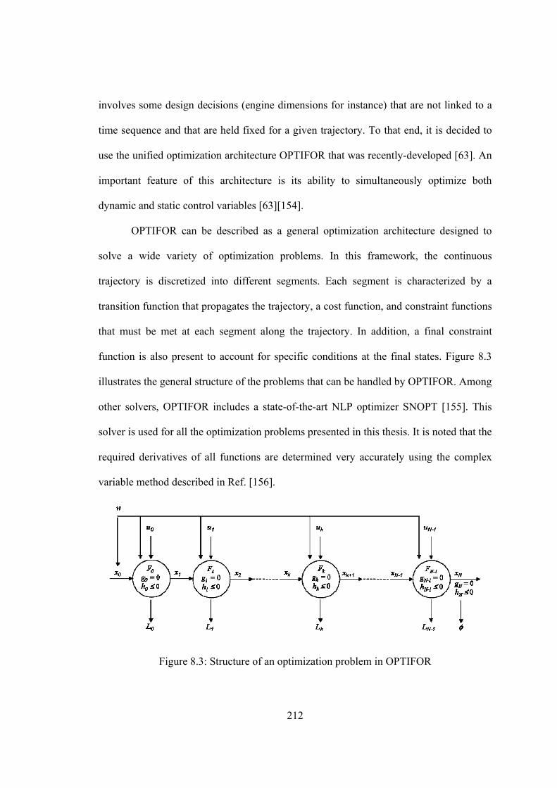
212
involves some design decisions (engine dimensions for instance) that are not linked to a
time sequence and that are held fixed for a given trajectory. To that end, it is decided to
use the unified optimization architecture OPTIFOR that was recently-developed [63]. An
important feature of this architecture is its ability to simultaneously optimize both
dynamic and static control variables [63][154].
OPTIFOR can be described as a general optimization architecture designed to
solve a wide variety of optimization problems. In this framework, the continuous
trajectory is discretized into different segments. Each segment is characterized by a
transition function that propagates the trajectory, a cost function, and constraint functions
that must be met at each segment along the trajectory. In addition, a final constraint
function is also present to account for specific conditions at the final states. Figure 8.3
illustrates the general structure of the problems that can be handled by OPTIFOR. Among
other solvers, OPTIFOR includes a state-of-the-art NLP optimizer SNOPT [155]. This
solver is used for all the optimization problems presented in this thesis. It is noted that the
required derivatives of all functions are determined very accurately using the complex
variable method described in Ref. [156].
Figure 8.3: Structure of an optimization problem in OPTIFOR
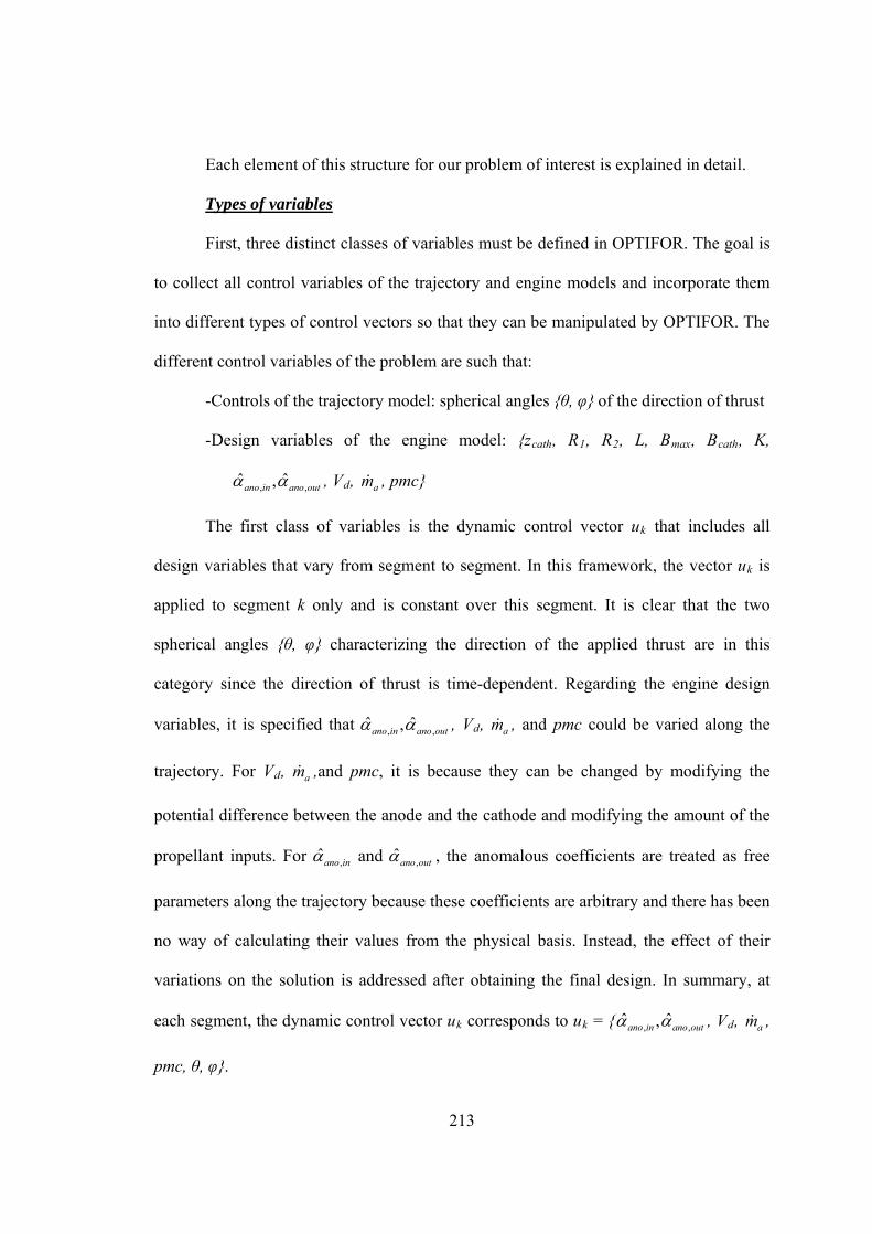
213
Each element of this structure for our problem of interest is explained in detail.
UTypes of variables
First, three distinct classes of variables must be defined in OPTIFOR. The goal is
to collect all control variables of the trajectory and engine models and incorporate them
into different types of control vectors so that they can be manipulated by OPTIFOR. The
different control variables of the problem are such that:
-Controls of the trajectory model: spherical angles {θ, φ} of the direction of thrust
-Design variables of the engine model: {zRcathR, RR1R, RR2R, L, BRmaxR, BRcathR, K,
, ,ˆ ˆ,ano in ano out , VRdR, am , pmc}
The first class of variables is the dynamic control vector uRkR that includes all
design variables that vary from segment to segment. In this framework, the vector uRkR is
applied to segment k only and is constant over this segment. It is clear that the two
spherical angles {θ, φ} characterizing the direction of the applied thrust are in this
category since the direction of thrust is time-dependent. Regarding the engine design
variables, it is specified that , ,ˆ ˆ,ano in ano out , VRdR, am , and pmc could be varied along the
trajectory. For VRdR, am ,and pmc, it is because they can be changed by modifying the
potential difference between the anode and the cathode and modifying the amount of the
propellant inputs. For ,ˆ
ano in and ,ˆ
ano out , the anomalous coefficients are treated as free
parameters along the trajectory because these coefficients are arbitrary and there has been
no way of calculating their values from the physical basis. Instead, the effect of their
variations on the solution is addressed after obtaining the final design. In summary, at
each segment, the dynamic control vector uRkR corresponds to uRkR = { , ,ˆ ˆ,ano in ano out , VRdR, am ,
pmc, θ, φ}.
214
The second variable class is the static control vector w that encompasses design
variables that can have an effect over the whole trajectory and are time-independent. This
includes obviously the variables related to the dimensions of the engine {zRcathR, RR1R, RR2R, L}.
In addition, it is also decided that BRmaxR, BRcathR, and K should be in this category as it is
assumed that changing them along the trajectory would be currently difficult. In
summary, the components of the static control vector are defined to be: w = {zRcathR, RR1R, RR2R,
L, BRmaxR, BRcathR, K}.
The last variable class is the time-dependent state vector x. It corresponds
classically to the position and velocity of the spacecraft, as well as its mass.
UTransition function
The representation of Sims and Flanegan is used to propagate the low-thrust
trajectory [157] - [158]. Each segment consists of a V impulse followed by a coast
period. The impulsive V s approximate the low thrust acceleration over a segment and
are computed from the corresponding thrust magnitude. The mass discontinuity due to
the impulse is obtained from the rocket equation. Thrust magnitude and IRspR are given by
the engine model. Figure 8.4 gives the flow diagram for the transition functions of the
segments.
Figure 8.4: Flow diagram of the transition function of a segment
215
UCost function
The cost function of each segment corresponds to the thrust magnitude, obtained
from the engine model.
USegment constraint functions
For feasibility, it should be guaranteed that the SVM constraint gR0R is met at each
segment. In addition, to account for the uncertainty in the anomalous coefficients, it is
decided that gR0R should be satisfied with some safety margin: gR0R ≥ lower limitd . The selection
of a proper value for lower limitd requires some trial-and-errors experiments, which will be
shown in the results section.
Moreover, even if other constraint functions gR1R, gR2R, gR3R, and gR4R generated by the
NNs using only thruster operation success cases are no longer strictly needed, they are
included to provide an extra safety strategy and to check their performance as constraints.
It is interesting to compare the behavior of gR1R, gR2R, gR3R, and gR4 Rwith the SVM constraint gR0R.
All extra constraints must be greater than 0 to indicate the feasible region.
Finally, the power usage required by the engine must not be greater than the
power available. In general, the power available is produced by solar arrays. To simplify
the problem, it is assumed that the power available is constant along the trajectory, which
is a good approximation for geocentric transfers since the distance from the Sun is nearly
constant. The corresponding constraint is therefore:
PRdR < PRavailableR , where PRdR is output power of the engine model.
The constraints which must be satisfied for each trajectory segment are
summarized in Table 8.2.
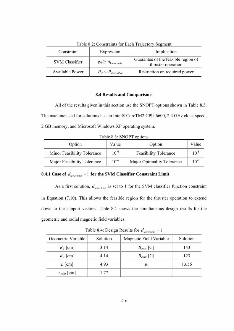
216
Table 8.2: Constraints for Each Trajectory Segment
Constraint Expression Implication
SVM Classifier gR0R ≥ lower limitd Guarantee of the feasible region of thruster operation
Available Power PRdR < PRavailable Restriction on required power
8.4 Results and Comparisons
All of the results given in this section use the SNOPT options shown in Table 8.3.
The machine used for solutions has an Intel® CoreTM2 CPU 6600, 2.4 GHz clock speed,
2 GB memory, and Microsoft Windows XP operating system.
Table 8.3: SNOPT options
Option Value Option Value
Minor Feasibility Tolerance 10 P
-6 Feasibility Tolerance 10P
-8
Major Feasibility Tolerance 10 P
-6 Major Optimality Tolerance 10P
-2
8.4.1 Case of lower limit 1d for the SVM Classifier Constraint Limit
As a first solution, lower limitd is set to 1 for the SVM classifier function constraint
in Equation (7.10). This allows the feasible region for the thruster operation to extend
down to the support vectors. Table 8.4 shows the simultaneous design results for the
geometric and radial magnetic field variables.
Table 8.4: Design Results for lower limit 1d
Geometric Variable Solution Magnetic Field Variable Solution
RR1R [cm] 3.14 BRmaxR [G] 143
RR2R [cm] 4.14 BRcathR [G] 123
L [cm] 4.93 K 13.56
zRcathR [cm] 1.77
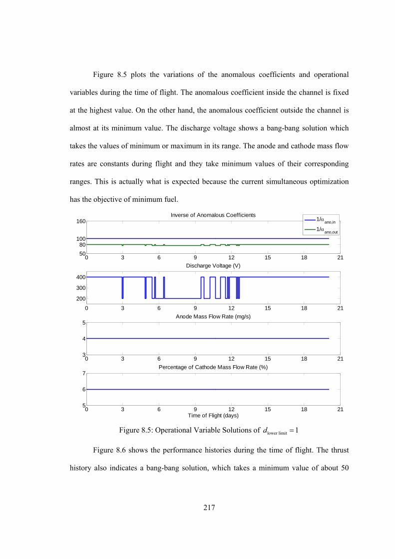
217
Figure 8.5 plots the variations of the anomalous coefficients and operational
variables during the time of flight. The anomalous coefficient inside the channel is fixed
at the highest value. On the other hand, the anomalous coefficient outside the channel is
almost at its minimum value. The discharge voltage shows a bang-bang solution which
takes the values of minimum or maximum in its range. The anode and cathode mass flow
rates are constants during flight and they take minimum values of their corresponding
ranges. This is actually what is expected because the current simultaneous optimization
has the objective of minimum fuel.
0 3 6 9 12 15 18 2150
80100
160Inverse of Anomalous Coefficients
1/ano,in
1/ano,out
0 3 6 9 12 15 18 21
200
300
400
Discharge Voltage (V)
0 3 6 9 12 15 18 213
4
5Anode Mass Flow Rate (mg/s)
0 3 6 9 12 15 18 215
6
7Percentage of Cathode Mass Flow Rate (%)
Time of Flight (days)
Figure 8.5: Operational Variable Solutions of lower limit 1d
Figure 8.6 shows the performance histories during the time of flight. The thrust
history also indicates a bang-bang solution, which takes a minimum value of about 50
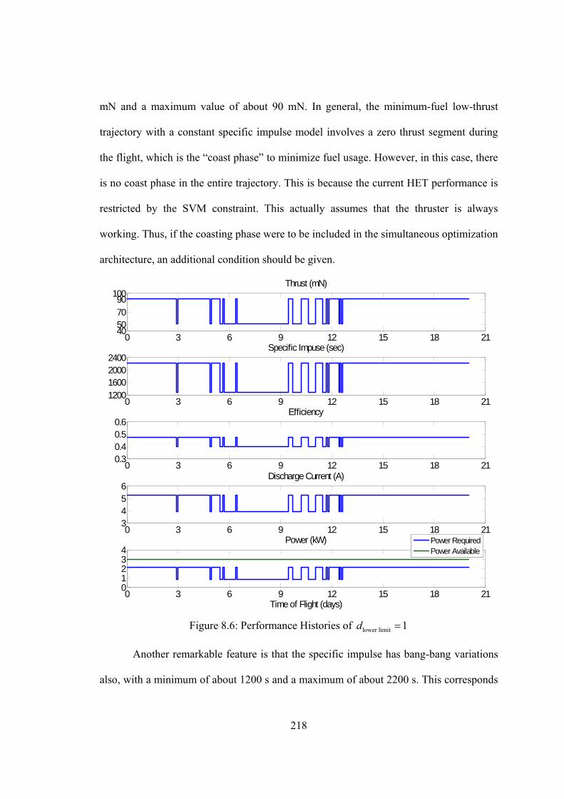
218
mN and a maximum value of about 90 mN. In general, the minimum-fuel low-thrust
trajectory with a constant specific impulse model involves a zero thrust segment during
the flight, which is the “coast phase” to minimize fuel usage. However, in this case, there
is no coast phase in the entire trajectory. This is because the current HET performance is
restricted by the SVM constraint. This actually assumes that the thruster is always
working. Thus, if the coasting phase were to be included in the simultaneous optimization
architecture, an additional condition should be given.
0 3 6 9 12 15 18 2140507090
100Thrust (mN)
0 3 6 9 12 15 18 211200160020002400
Specific Impuse (sec)
0 3 6 9 12 15 18 210.30.40.50.6
Efficiency
0 3 6 9 12 15 18 213456
Discharge Current (A)
0 3 6 9 12 15 18 2101234
Power (kW)
Time of Flight (days)
Power RequiredPower Available
Figure 8.6: Performance Histories of lower limit 1d
Another remarkable feature is that the specific impulse has bang-bang variations
also, with a minimum of about 1200 s and a maximum of about 2200 s. This corresponds
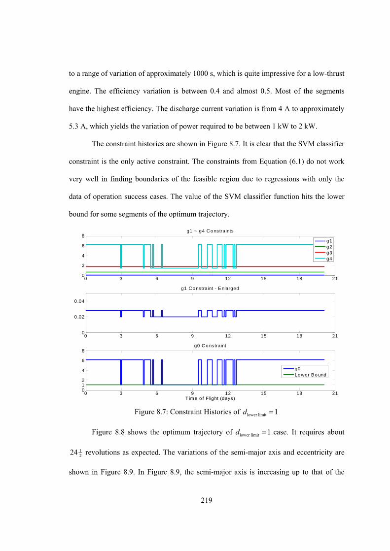
219
to a range of variation of approximately 1000 s, which is quite impressive for a low-thrust
engine. The efficiency variation is between 0.4 and almost 0.5. Most of the segments
have the highest efficiency. The discharge current variation is from 4 A to approximately
5.3 A, which yields the variation of power required to be between 1 kW to 2 kW.
The constraint histories are shown in Figure 8.7. It is clear that the SVM classifier
constraint is the only active constraint. The constraints from Equation (6.1) do not work
very well in finding boundaries of the feasible region due to regressions with only the
data of operation success cases. The value of the SVM classifier function hits the lower
bound for some segments of the optimum trajectory.
0 3 6 9 12 15 18 210
2
4
6
8g1 ~ g4 Co nstraints
g1g2g3g4
0 3 6 9 12 15 18 210
0.02
0.04
g1 Co nstraint - E nlarged
0 3 6 9 12 15 18 21012
4
6
8g0 C o nstraint
T ime o f Flight (days)
g0Lo wer B o und
Figure 8.7: Constraint Histories of lower limit 1d
Figure 8.8 shows the optimum trajectory of lower limit 1d case. It requires about
1224 revolutions as expected. The variations of the semi-major axis and eccentricity are
shown in Figure 8.9. In Figure 8.9, the semi-major axis is increasing up to that of the
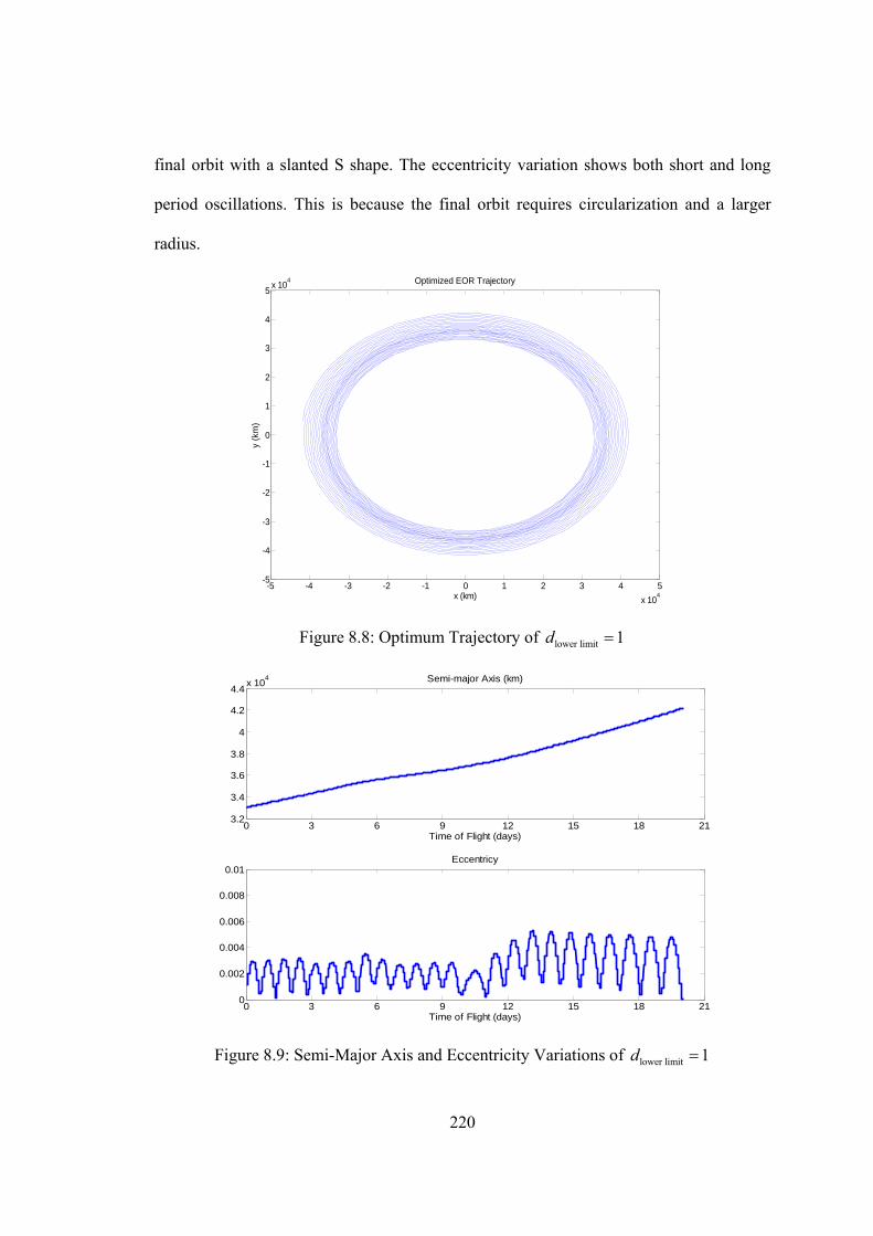
220
final orbit with a slanted S shape. The eccentricity variation shows both short and long
period oscillations. This is because the final orbit requires circularization and a larger
radius.
-5 -4 -3 -2 -1 0 1 2 3 4 5
x 104
-5
-4
-3
-2
-1
0
1
2
3
4
5x 10
4
x (km)
y (k
m)
Optimized EOR Trajectory
Figure 8.8: Optimum Trajectory of lower limit 1d
0 3 6 9 12 15 18 213.2
3.4
3.6
3.8
4
4.2
4.4x 10
4 Semi-major Axis (km)
Time of Flight (days)
0 3 6 9 12 15 18 210
0.002
0.004
0.006
0.008
0.01Eccentricy
Time of Flight (days)
Figure 8.9: Semi-Major Axis and Eccentricity Variations of lower limit 1d
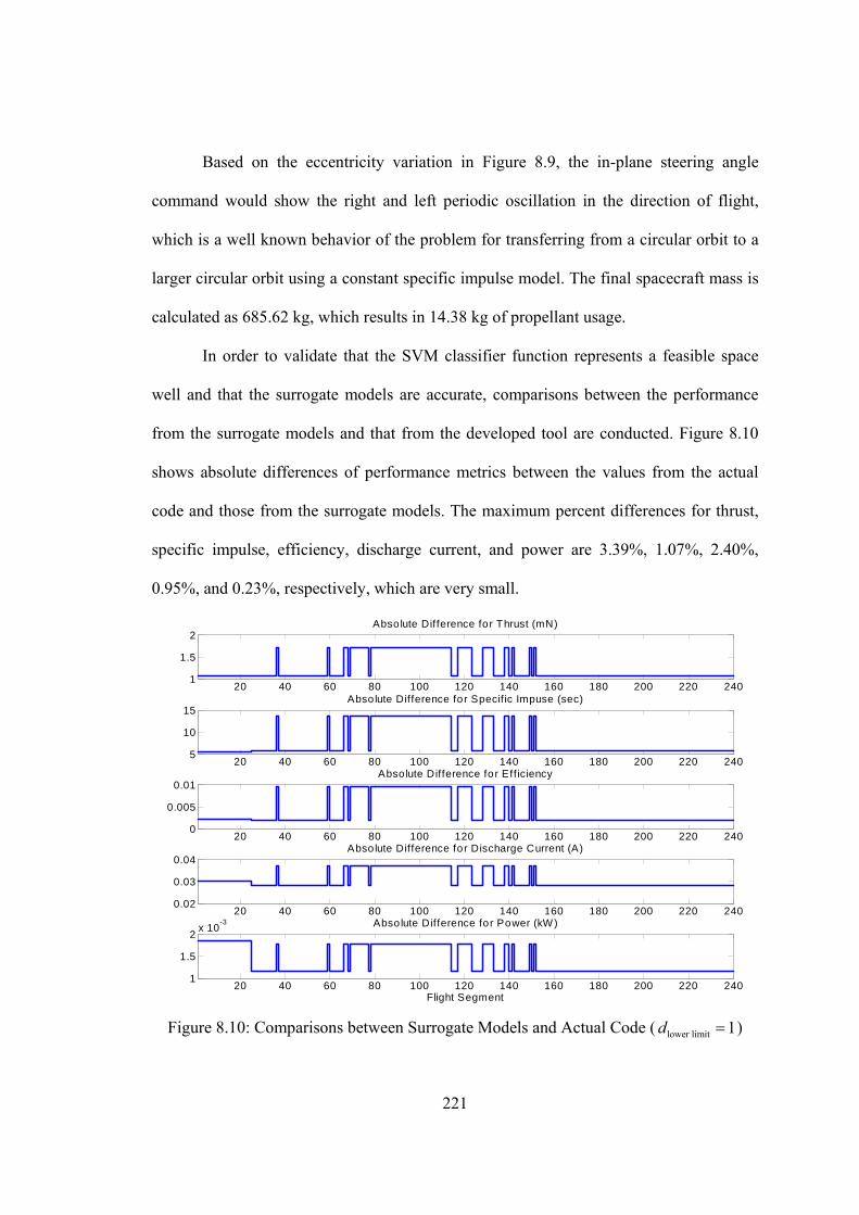
221
Based on the eccentricity variation in Figure 8.9, the in-plane steering angle
command would show the right and left periodic oscillation in the direction of flight,
which is a well known behavior of the problem for transferring from a circular orbit to a
larger circular orbit using a constant specific impulse model. The final spacecraft mass is
calculated as 685.62 kg, which results in 14.38 kg of propellant usage.
In order to validate that the SVM classifier function represents a feasible space
well and that the surrogate models are accurate, comparisons between the performance
from the surrogate models and that from the developed tool are conducted. Figure 8.10
shows absolute differences of performance metrics between the values from the actual
code and those from the surrogate models. The maximum percent differences for thrust,
specific impulse, efficiency, discharge current, and power are 3.39%, 1.07%, 2.40%,
0.95%, and 0.23%, respectively, which are very small.
20 40 60 80 100 120 140 160 180 200 220 2401
1.5
2Absolute Difference for Thrust (mN)
20 40 60 80 100 120 140 160 180 200 220 2405
10
15Absolute Difference for Specif ic Impuse (sec)
20 40 60 80 100 120 140 160 180 200 220 2400
0.005
0.01Absolute Difference for Efficiency
20 40 60 80 100 120 140 160 180 200 220 2400.02
0.03
0.04Absolute Difference for Discharge Current (A)
20 40 60 80 100 120 140 160 180 200 220 2401
1.5
2x 10
-3 Absolute Difference for Power (kW)
Flight Segment
Figure 8.10: Comparisons between Surrogate Models and Actual Code ( lower limit 1d )
222
As shown in Figure 8.10, the developed tool produces all of the responses for
optimum geometry, radial magnetic field parameters, and the variations of operational
variables. This indicates that the optimum solutions are within the feasible region. This
also confirms that the SVM classifier function constraint is well performing.
Because the anomalous coefficients are arbitrary values, the optimum solutions
from the simultaneous design optimization must be given in terms of probability of
success and confidence. For this purpose, a Monte Carlo simulation is required for the
anomalous coefficients. The strategy is that for each segment of the optimal trajectory
10000 pairs of the anomalous coefficients are randomly generated. The generated pairs
for each segment are then checked with the SVM classifier constraint. In this case,
lower limitd is set to zero to cover the entire feasible region. This provides the probability of
success (or the success rate) of the obtained optimum solution. The performance values
are then calculated with the pairs which do not violate the SVM classifier constraint.
Trajectories are integrated with these feasible cases. The required confidence can be
given by the distributions of the orbital elements at the end state and the final spacecraft
mass.
Unfortunately, results of the Monte Carlo simulation show that the probability of
success is 0 for the case of lower limit 1d . This means that a harder limit should be given to
the SVM classifier constraint in order to address the arbitrary variations of the anomalous
coefficients. As a result, the harder limit will reduce the feasible region of the thruster
operation.
8.4.2 Case of lower limit 3d for the SVM Classifier Constraint Limit
223
The limit for the SVM classifier constraint is now set to 3. This reduces the
feasible space for the thruster operation compared to the previous case. The convergence
properties are shown in Table 8.5.
Table 8.5: Convergence Property for lower limit 3d
Iteration CPU Run Time Max Constraint Violation No. of Iteration: 5751
No. of Function Calls: 136 21.35 min. 1.0×10P
-5
Table 8.6 shows the simultaneous design results for the geometric and radial
magnetic field variables.
Table 8.6: Design Results for lower limit 3d
Geometric Variable Solution Magnetic Field Variable Solution
RR1R [cm] 3.54 BRmaxR [Gauss] 157
RR2R [cm] 4.54 BRcathR [Gauss] 137
L [cm] 5.00 K 13.99
zRcathR [cm] 1.92
Both the inner and outer radii are slightly increased. The cathode location is a
little farther from the thrust exit line than before. The maximum and the cathode radial
magnetic fields are increased by about 15 Gauss. The magnetic field shape coefficient is
almost the same as the previous case.
Figure 8.11 plots the variations of the anomalous coefficients and operational
variables during the time of flight. The anomalous electron diffusion inside the channel is
slightly decreased. Again, the discharge voltage shows more bang-bang behavior. It is
also clearly seen that the range of the discharge voltage variation is reduced by 100 V, to
between 300 V and 400 V. This is because the feasible design space for the optimization
is reduced by the SVM classifier constraint. The anode and cathode mass flow rates still
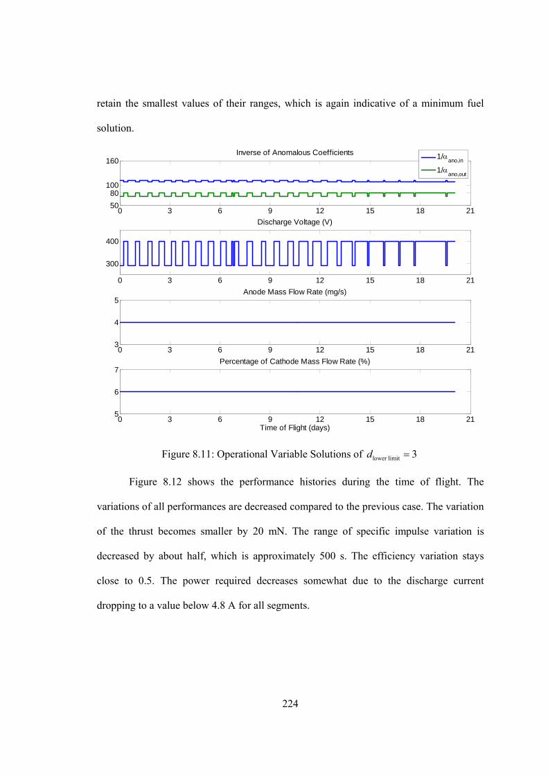
224
retain the smallest values of their ranges, which is again indicative of a minimum fuel
solution.
0 3 6 9 12 15 18 2150
80100
160Inverse of Anomalous Coefficients
1/
ano,in
1/ano,out
0 3 6 9 12 15 18 21
300
400
Discharge Voltage (V)
0 3 6 9 12 15 18 213
4
5Anode Mass Flow Rate (mg/s)
0 3 6 9 12 15 18 215
6
7Percentage of Cathode Mass Flow Rate (%)
Time of Flight (days)
Figure 8.11: Operational Variable Solutions of lower limit 3d
Figure 8.12 shows the performance histories during the time of flight. The
variations of all performances are decreased compared to the previous case. The variation
of the thrust becomes smaller by 20 mN. The range of specific impulse variation is
decreased by about half, which is approximately 500 s. The efficiency variation stays
close to 0.5. The power required decreases somewhat due to the discharge current
dropping to a value below 4.8 A for all segments.
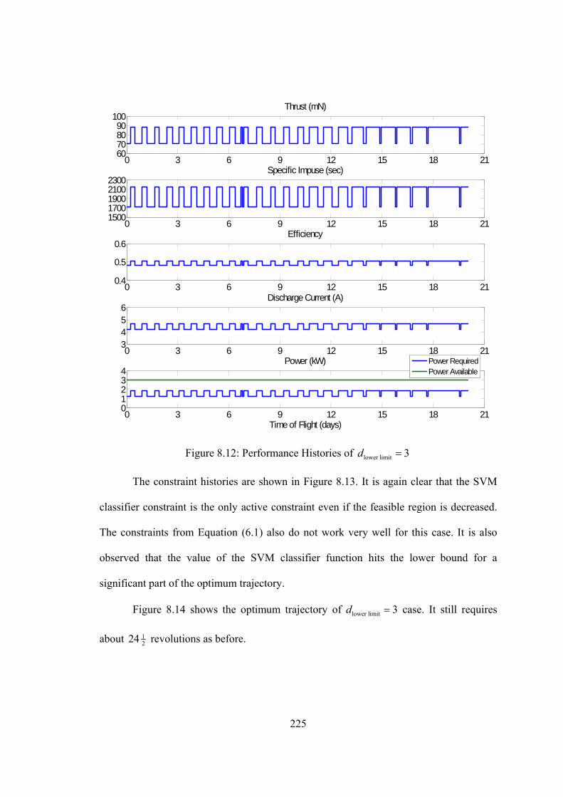
225
0 3 6 9 12 15 18 2160708090
100Thrust (mN)
0 3 6 9 12 15 18 2115001700190021002300
Specific Impuse (sec)
0 3 6 9 12 15 18 210.4
0.5
0.6Efficiency
0 3 6 9 12 15 18 213456
Discharge Current (A)
0 3 6 9 12 15 18 2101234
Power (kW)
Time of Flight (days)
Power RequiredPower Available
Figure 8.12: Performance Histories of lower limit 3d
The constraint histories are shown in Figure 8.13. It is again clear that the SVM
classifier constraint is the only active constraint even if the feasible region is decreased.
The constraints from Equation (6.1) also do not work very well for this case. It is also
observed that the value of the SVM classifier function hits the lower bound for a
significant part of the optimum trajectory.
Figure 8.14 shows the optimum trajectory of lower limit 3d case. It still requires
about 1224 revolutions as before.
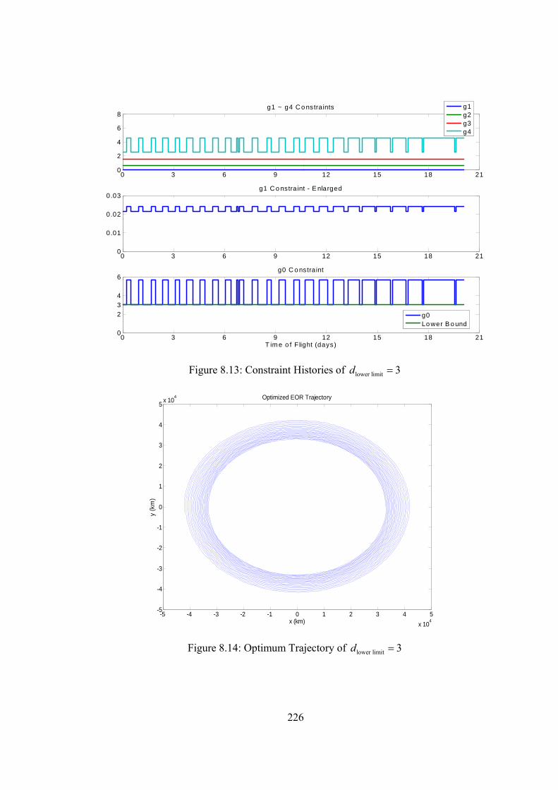
226
0 3 6 9 12 15 18 210
2
4
6
8g1 ~ g4 C o nstraints
g1g2g3g4
0 3 6 9 12 15 18 210
0.01
0.02
0.03g1 C o nstraint - E nlarged
0 3 6 9 12 15 18 210
2
3
4
6g0 C o nstraint
T im e o f Flight (days)
g0Lo wer B o und
Figure 8.13: Constraint Histories of lower limit 3d
-5 -4 -3 -2 -1 0 1 2 3 4 5
x 104
-5
-4
-3
-2
-1
0
1
2
3
4
5x 10
4
x (km)
y (k
m)
Optimized EOR Trajectory
Figure 8.14: Optimum Trajectory of lower limit 3d
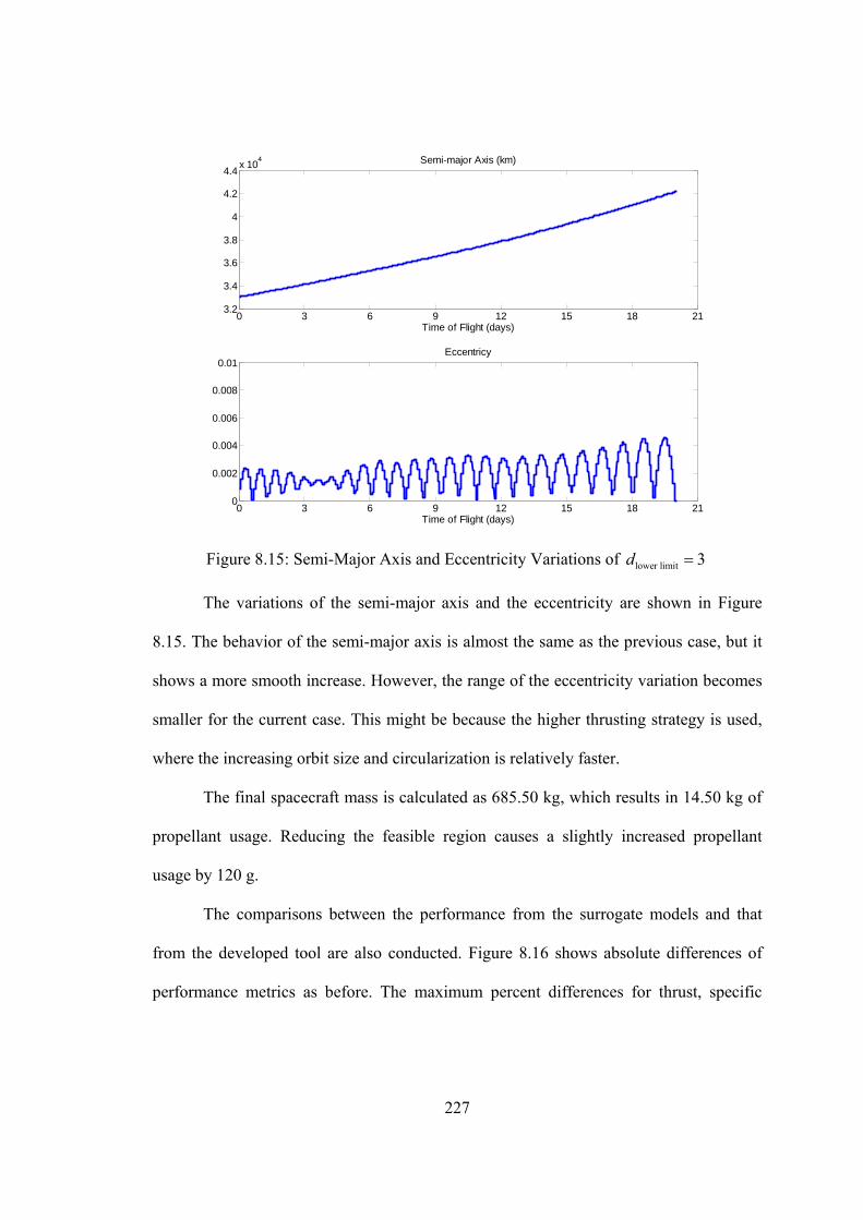
227
0 3 6 9 12 15 18 213.2
3.4
3.6
3.8
4
4.2
4.4x 10
4 Semi-major Axis (km)
Time of Flight (days)
0 3 6 9 12 15 18 210
0.002
0.004
0.006
0.008
0.01Eccentricy
Time of Flight (days)
Figure 8.15: Semi-Major Axis and Eccentricity Variations of lower limit 3d
The variations of the semi-major axis and the eccentricity are shown in Figure
8.15. The behavior of the semi-major axis is almost the same as the previous case, but it
shows a more smooth increase. However, the range of the eccentricity variation becomes
smaller for the current case. This might be because the higher thrusting strategy is used,
where the increasing orbit size and circularization is relatively faster.
The final spacecraft mass is calculated as 685.50 kg, which results in 14.50 kg of
propellant usage. Reducing the feasible region causes a slightly increased propellant
usage by 120 g.
The comparisons between the performance from the surrogate models and that
from the developed tool are also conducted. Figure 8.16 shows absolute differences of
performance metrics as before. The maximum percent differences for thrust, specific
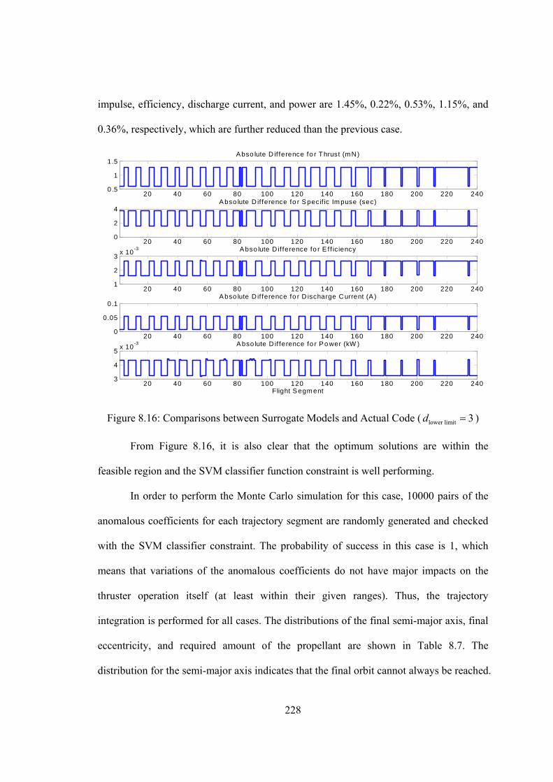
228
impulse, efficiency, discharge current, and power are 1.45%, 0.22%, 0.53%, 1.15%, and
0.36%, respectively, which are further reduced than the previous case.
20 40 60 80 100 120 140 160 180 200 220 2400.5
1
1.5A bso lute D if ference fo r T hrust (m N)
20 40 60 80 100 120 140 160 180 200 220 2400
2
4A bso lute D if ference fo r S pecif ic Im puse (sec)
20 40 60 80 100 120 140 160 180 200 220 2401
2
3x 10
-3 A bso lute D if ference fo r E ff ic iency
20 40 60 80 100 120 140 160 180 200 220 2400
0.05
0.1A bso lute D if ference fo r D ischarge C urrent (A )
20 40 60 80 100 120 140 160 180 200 220 2403
4
5x 10
-3 A bso lute D if ference fo r P o wer (kW )
Flight S egm ent
Figure 8.16: Comparisons between Surrogate Models and Actual Code ( lower limit 3d )
From Figure 8.16, it is also clear that the optimum solutions are within the
feasible region and the SVM classifier function constraint is well performing.
In order to perform the Monte Carlo simulation for this case, 10000 pairs of the
anomalous coefficients for each trajectory segment are randomly generated and checked
with the SVM classifier constraint. The probability of success in this case is 1, which
means that variations of the anomalous coefficients do not have major impacts on the
thruster operation itself (at least within their given ranges). Thus, the trajectory
integration is performed for all cases. The distributions of the final semi-major axis, final
eccentricity, and required amount of the propellant are shown in Table 8.7. The
distribution for the semi-major axis indicates that the final orbit cannot always be reached.
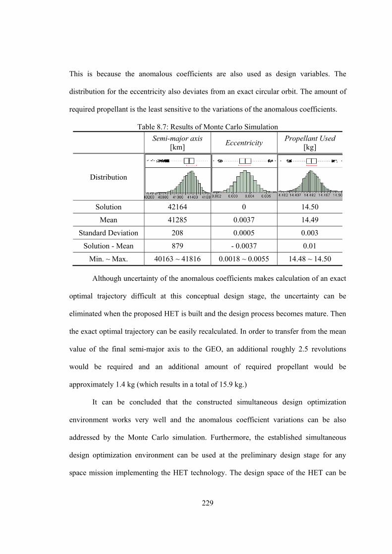
229
This is because the anomalous coefficients are also used as design variables. The
distribution for the eccentricity also deviates from an exact circular orbit. The amount of
required propellant is the least sensitive to the variations of the anomalous coefficients.
Table 8.7: Results of Monte Carlo Simulation
Semi-major axis
[km] Eccentricity
Propellant Used [kg]
Distribution
Solution 42164 0 14.50
Mean 41285 0.0037 14.49
Standard Deviation 208 0.0005 0.003
Solution - Mean 879 - 0.0037 0.01
Min. ~ Max. 40163 ~ 41816 0.0018 ~ 0.0055 14.48 ~ 14.50
Although uncertainty of the anomalous coefficients makes calculation of an exact
optimal trajectory difficult at this conceptual design stage, the uncertainty can be
eliminated when the proposed HET is built and the design process becomes mature. Then
the exact optimal trajectory can be easily recalculated. In order to transfer from the mean
value of the final semi-major axis to the GEO, an additional roughly 2.5 revolutions
would be required and an additional amount of required propellant would be
approximately 1.4 kg (which results in a total of 15.9 kg.)
It can be concluded that the constructed simultaneous design optimization
environment works very well and the anomalous coefficient variations can be also
addressed by the Monte Carlo simulation. Furthermore, the established simultaneous
design optimization environment can be used at the preliminary design stage for any
space mission implementing the HET technology. The design space of the HET can be
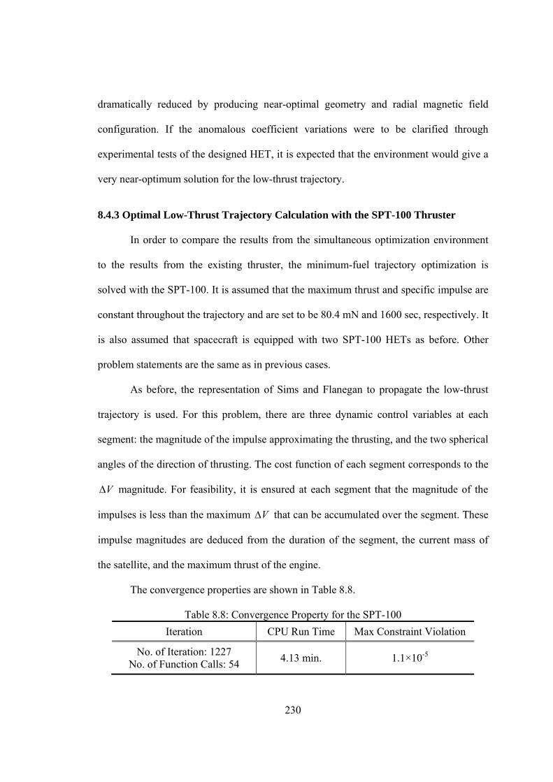
230
dramatically reduced by producing near-optimal geometry and radial magnetic field
configuration. If the anomalous coefficient variations were to be clarified through
experimental tests of the designed HET, it is expected that the environment would give a
very near-optimum solution for the low-thrust trajectory.
8.4.3 Optimal Low-Thrust Trajectory Calculation with the SPT-100 Thruster
In order to compare the results from the simultaneous optimization environment
to the results from the existing thruster, the minimum-fuel trajectory optimization is
solved with the SPT-100. It is assumed that the maximum thrust and specific impulse are
constant throughout the trajectory and are set to be 80.4 mN and 1600 sec, respectively. It
is also assumed that spacecraft is equipped with two SPT-100 HETs as before. Other
problem statements are the same as in previous cases.
As before, the representation of Sims and Flanegan to propagate the low-thrust
trajectory is used. For this problem, there are three dynamic control variables at each
segment: the magnitude of the impulse approximating the thrusting, and the two spherical
angles of the direction of thrusting. The cost function of each segment corresponds to the
V magnitude. For feasibility, it is ensured at each segment that the magnitude of the
impulses is less than the maximum V that can be accumulated over the segment. These
impulse magnitudes are deduced from the duration of the segment, the current mass of
the satellite, and the maximum thrust of the engine.
The convergence properties are shown in Table 8.8.
Table 8.8: Convergence Property for the SPT-100
Iteration CPU Run Time Max Constraint Violation
No. of Iteration: 1227 No. of Function Calls: 54
4.13 min. 1.1×10P
-5
231
Figure 8.17 shows the thrust history. The thrust takes the maximum value for
entire trajectory segments, which indicates a constant maximum thrusting strategy. This
strategy is typically observed in minimum time solutions. As explained in section 8.2, the
time of flight is fixed as that of the minimum time solution using the SPT-100. When the
time of flight is chosen greater than the minimum time of the SPT-100 solution, the
minimum fuel solution of the SPT-100 would produce some coasting phases. However,
the engine model in the current simultaneous optimization architecture doesn’t allow
coasting phases due to the SVM constraint, which enforces no coasting phases on the
minimum fuel solution of the SPT-100 as well. Therefore, it is clear that the minimum
fuel solution of the SPT-100 should be the same as the minimum time solution of the
SPT-100.
0 3 6 9 12 15 18 2170
72
74
76
78
80
82
84
86
88
90
Time of Flight (days)
Thr
ust (
mN
)
Figure 8.17: Thrust History for the SPT-100
Figure 8.18 shows the optimum EOR trajectory using the SPT-100. The
revolution is almost the same as before due to the fixed time of flight. Figure 8.19 shows
the semi-major axis and the eccentricity variations with time. The semi-major axis
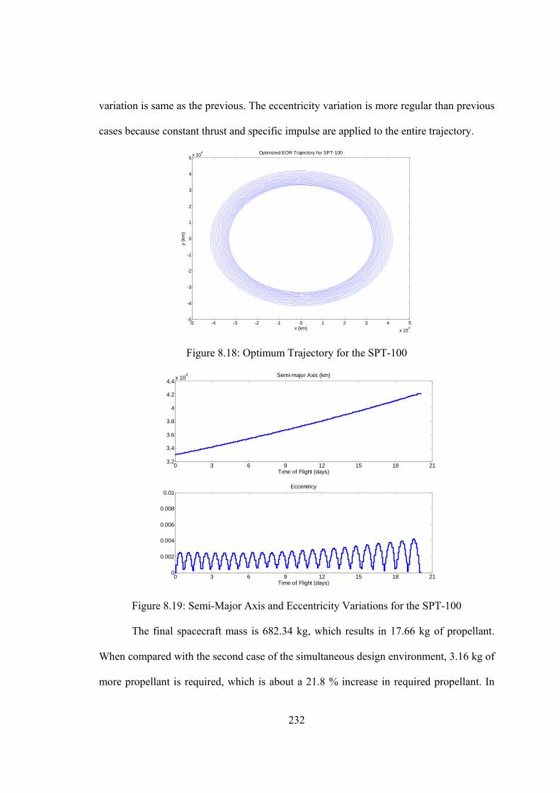
232
variation is same as the previous. The eccentricity variation is more regular than previous
cases because constant thrust and specific impulse are applied to the entire trajectory.
-5 -4 -3 -2 -1 0 1 2 3 4 5
x 104
-5
-4
-3
-2
-1
0
1
2
3
4
5x 10
4
x (km)
y (k
m)
Optimized EOR Trajectory for SPT-100
Figure 8.18: Optimum Trajectory for the SPT-100
0 3 6 9 12 15 18 213.2
3.4
3.6
3.8
4
4.2
4.4x 10
4 Semi-major Axis (km)
Time of Flight (days)
0 3 6 9 12 15 18 210
0.002
0.004
0.006
0.008
0.01Eccentricy
Time of Flight (days)
Figure 8.19: Semi-Major Axis and Eccentricity Variations for the SPT-100
The final spacecraft mass is 682.34 kg, which results in 17.66 kg of propellant.
When compared with the second case of the simultaneous design environment, 3.16 kg of
more propellant is required, which is about a 21.8 % increase in required propellant. In
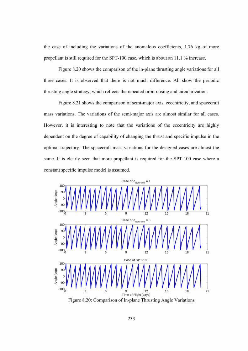
233
the case of including the variations of the anomalous coefficients, 1.76 kg of more
propellant is still required for the SPT-100 case, which is about an 11.1 % increase.
Figure 8.20 shows the comparison of the in-plane thrusting angle variations for all
three cases. It is observed that there is not much difference. All show the periodic
thrusting angle strategy, which reflects the repeated orbit raising and circularization.
Figure 8.21 shows the comparison of semi-major axis, eccentricity, and spacecraft
mass variations. The variations of the semi-major axis are almost similar for all cases.
However, it is interesting to note that the variations of the eccentricity are highly
dependent on the degree of capability of changing the thrust and specific impulse in the
optimal trajectory. The spacecraft mass variations for the designed cases are almost the
same. It is clearly seen that more propellant is required for the SPT-100 case where a
constant specific impulse model is assumed.
0 3 6 9 12 15 18 21-180
-90
0
90
180
Case of dlower limit
= 1
Ang
le (
deg)
0 3 6 9 12 15 18 21-180
-90
0
90
180
Case of dlower limit
= 3
Ang
le (
deg)
0 3 6 9 12 15 18 21-180
-90
0
90
180Case of SPT-100
Ang
le (
deg)
Time of Flight (days) Figure 8.20: Comparison of In-plane Thrusting Angle Variations
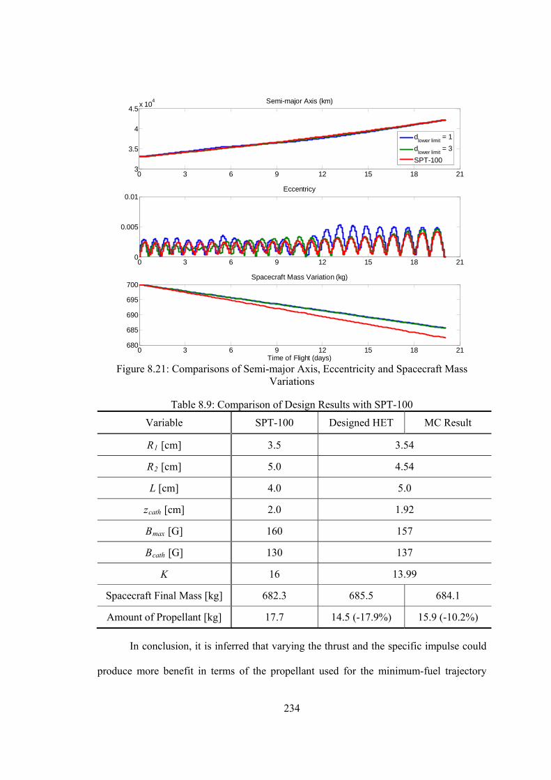
234
0 3 6 9 12 15 18 213
3.5
4
4.5x 10
4 Semi-major Axis (km)
dlower limit
= 1
dlower limit
= 3
SPT-100
0 3 6 9 12 15 18 210
0.005
0.01Eccentricy
0 3 6 9 12 15 18 21680
685
690
695
700Spacecraft Mass Variation (kg)
Time of Flight (days) Figure 8.21: Comparisons of Semi-major Axis, Eccentricity and Spacecraft Mass
Variations
Table 8.9: Comparison of Design Results with SPT-100
Variable SPT-100 Designed HET MC Result
RR1R [cm] 3.5 3.54
RR2R [cm] 5.0 4.54
L [cm] 4.0 5.0
zRcathR [cm] 2.0 1.92
BRmaxR [G] 160 157
BRcathR [G] 130 137
K 16 13.99
Spacecraft Final Mass [kg] 682.3 685.5 684.1
Amount of Propellant [kg] 17.7 14.5 (-17.9%) 15.9 (-10.2%)
In conclusion, it is inferred that varying the thrust and the specific impulse could
produce more benefit in terms of the propellant used for the minimum-fuel trajectory
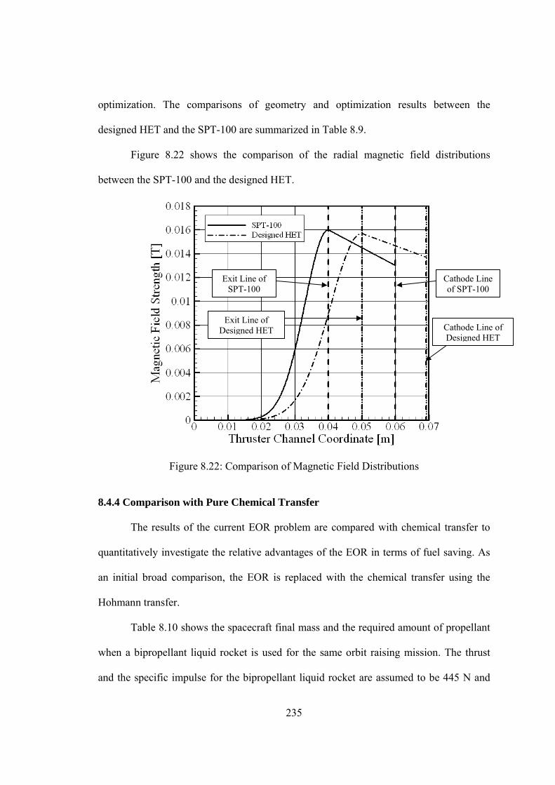
235
optimization. The comparisons of geometry and optimization results between the
designed HET and the SPT-100 are summarized in Table 8.9.
Figure 8.22 shows the comparison of the radial magnetic field distributions
between the SPT-100 and the designed HET.
Figure 8.22: Comparison of Magnetic Field Distributions
8.4.4 Comparison with Pure Chemical Transfer
The results of the current EOR problem are compared with chemical transfer to
quantitatively investigate the relative advantages of the EOR in terms of fuel saving. As
an initial broad comparison, the EOR is replaced with the chemical transfer using the
Hohmann transfer.
Table 8.10 shows the spacecraft final mass and the required amount of propellant
when a bipropellant liquid rocket is used for the same orbit raising mission. The thrust
and the specific impulse for the bipropellant liquid rocket are assumed to be 445 N and
Exit Line of SPT-100
Exit Line of Designed HET
Cathode Line of SPT-100
Cathode Line of Designed HET
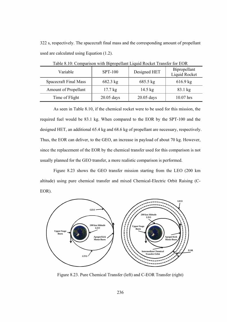
236
322 s, respectively. The spacecraft final mass and the corresponding amount of propellant
used are calculated using Equation (1.2).
Table 8.10: Comparison with Bipropellant Liquid Rocket Transfer for EOR
Variable SPT-100 Designed HET Bipropellant
Liquid Rocket
Spacecraft Final Mass 682.3 kg 685.5 kg 616.9 kg
Amount of Propellant 17.7 kg 14.5 kg 83.1 kg
Time of Flight 20.05 days 20.05 days 10.07 hrs
As seen in Table 8.10, if the chemical rocket were to be used for this mission, the
required fuel would be 83.1 kg. When compared to the EOR by the SPT-100 and the
designed HET, an additional 65.4 kg and 68.6 kg of propellant are necessary, respectively.
Thus, the EOR can deliver, to the GEO, an increase in payload of about 70 kg. However,
since the replacement of the EOR by the chemical transfer used for this comparison is not
usually planned for the GEO transfer, a more realistic comparison is performed.
Figure 8.23 shows the GEO transfer mission starting from the LEO (200 km
altitude) using pure chemical transfer and mixed Chemical-Electric Orbit Raising (C-
EOR).
200 km AltitudeLEO
GTO
GEO
Upper StageBurn
Apogee KickMotor Burn
200 km AltitudeLEO
Intermediate ChemicalTransfer Orbit
GEO
Upper StageBurn
Apogee KickMotor Burn
EOR
Figure 8.23. Pure Chemical Transfer (left) and C-EOR Transfer (right)
237
The pure chemical transfer scenario is as follows; 1) the upper stage burn delivers
the spacecraft into the GTO, and 2) the apogee kick motor burn inserts the spacecraft to
the final GEO. The pure chemical transfer is also using the Hohmann transfer to
minimize the required fuel. The upper stage of the Sea Launch is the Block DM-SL,
where the propulsive capability is provided by the 11D58M rocket. The rocket uses liquid
oxygen and kerosene. The thrust and the specific impulse are assumed to be 80 kN and
353 s, respectively. The C-EOR mission phases are given in section 8.2.
In order to compare these two transfer strategies, the total required fuel for each
case is calculated to deliver a given final mass. The given final mass is chosen to be
685.5 kg, which is the final mass for the case of the designed HET. The comparison
results are shown in Table 8.11.
Table 8.11: Comparison of Pure Chemical Transfer and C-EOR
Variable Pure Chemical Transfer C-EOR
Amount of Propellant 1538.4 kg 1462.5 kg
Spacecraft Initial Mass 2223.9 kg 2148.0 kg
Time of Flight 5.26 hrs 20.21 days
As seen in Table 8.11, the C-EOR can save about 76 kg of fuel, which means that
the C-EOR can deliver about 76 kg more payload to the GEO with the same initial
spacecraft mass of the pure chemical transfer. Comparing Table 8.11 with Table 8.10, the
main advantage of fuel saving results from the EOR. In order to obtain a broad estimate
for cost savings, the cost savings per unit of delivered mass is calculated based on data in
Ref. [151], which is shown in Table 8.12.
238
Table 8.12: GEO Delivery Cost Estimation [151]
BOL Mass [kg] Strategy Cost [M$] Cost Savings per Unit
Delivered Mass [M$/kg]
3445 Proton M/Breeze M + EOR 82
0.0023 Sea Launch w/o EOR 90
4073 Sea Launch + EOR 106
0.0034 Ariane 5 w/o EOR 120
If the average value of the cost savings per unit of delivered mass is used, about
0.22 M$ could be saved for this case with the designed HET. It is clear from these
comparisons that the advantage of SEP is considerable in terms of fuel savings (mass
transportation) and cost, although the transfer time is a lot longer than that of the
chemical rocket.

239
CHAPTER 9
CONCLUSIONS AND FUTURE WORK
9.1 Conclusions
The motivations come from the needs for improving the current expensive
experimental design procedure and infusing the actual HET performance envelope in the
low-thrust trajectory optimization. The observations on the current design process of the
HETs and the low-thrust trajectory optimization are made and the initial main questions
are recalled here:
Observation A. The design process of the HETs has relied on mostly an
experimental and empirical process.
Q1: How can the conceptual design process of HET be improved?
Observation B. The low-thrust trajectory optimization has been performed
without consideration of the performance envelope of a real electric thruster.
Q2: How can the real thruster performance be infused in preliminary low-thrust
trajectory optimization for a specific space mission?
Observation C. The design of HETs and the associated low-thrust trajectory
optimization has been decoupled.
Q3: How can the simultaneous design optimization environment be constructed?
The main questions guide the direction of the current research. In order to answer
the main questions, subsequent secondary questions arise and are as follows:
240
Q4: Can an appropriate physics-based tool or methodology at the conceptual
level be found among existing tools or methodologies?
Q5: If not, what is required to develop an appropriate physics-based tool or
methodology?
In order to answer Q4 and Q5, there is a need for a proper physics-based analysis
tool or methodology at a conceptual level of design. Thus, addressing this need is the first
objective of the thesis, which is recalled here:
O1: Identify a proper physics-based analysis tool or methodology for general
HET performances among existing methods, which fits at the conceptual design level
for HET. If an adequate tool or methodology were not identified, develop an
appropriate tool or methodology which meets the current research purposes.
The first objective requires the proposition of four criteria such as numerical
efficiency, numerical robustness, self-consistency, and physics representativeness to
evaluate the current tools or methodologies. Based on the evaluation in section 3.3, none
are identified as an appropriate tool. Thus, a proper tool is developed with a new
approach where the main idea is two-region discharge characterizing the HET physics.
The development of a new tool can be achieved by addressing the hypotheses, which are
repeated here.
Hypothesis 1. If the highly detail physics can be properly omitted when providing
macroscopic performance metrics, the fluid approach will be a good candidate for
improving numerical efficiency.
Hypothesis 2. If the singular form of a system of ODEs occurring in fluid
approach can be somehow avoided, numerical robustness will be improved.
241
Hypothesis 3. If proper modeling near the anode region is included in the fluid
approach, a self-consistent model will be constructed and the number of arbitrary
boundary conditions will be reduced.
Hypothesis 4. If most of the major physical phenomena are included in the model
and all concerned variables are computed by the tool within the range of assumptions, the
tool will represent sufficient physical phenomena experimentally observed in HET.
The application of the fluid approach ensures the numerical efficiency as proved
in the SPT-100 point validation. The idea of the two-region discharge makes it possible
to avoid the singular form of the system of ODEs and have no dependence on the initial
conditions for solutions, which results in the numerical robustness. The simple anode
modeling introduced in section 4.3.4 enables the developed tool to solve all dependent
variables without inputting arbitrary values, which guarantees the self-consistency.
Finally, as seen in section 5.1, most of major physical phenomena are well reproduced by
the developed tool with high accuracy of the performance metrics, which provides the
moderate HET physics representativeness. At this point, another secondary question
arises.
Q6: In case of developing an appropriate tool, can it be validated for a variety of
existing HETs?
Q6 is answered by the intensive validation and additional capability studies which
justifies the possibility of its use for new HET designs in spite of uncertainties in the
anomalous coefficients. This achievement is largely attributed to careful examination of
HET plasma physics from previous researches. This can lead to physical intuitions which
give birth to new ideas as well as proofs of the proposed hypotheses.

242
In order to answer Q2 and Q3, the following secondary questions are invoked:
Q7: Can the appropriate tool be efficiently used for the simultaneous design
optimization?
Q8: Can the feasible design space of HET to be designed be properly specified
for the simultaneous design optimization.
The second and third objectives are intended to answer these questions by
providing an HET performance analysis module that can be used for the simultaneous
design environment, which are repeated here:
O2: Perform conceptual design space exploration for performance metrics with
the identified or developed analysis tool. This task is expected to provide more thorough
information for a new design of HETs in terms of thruster performance. In addition, a
more broad understanding of HET is expected to be gained.
O3: Build the HET performance analysis module based on the identified or
developed HET analysis tool and clearly identify the feasible HET design space for the
simultaneous design optimization with the low-thrust trajectory optimization.
Based on the validation experience, a proper design space for the intended space
missions can be defined. Furthermore, the analysis of DSE results provides several
important observations on the thruster performance in terms of design variables such as
identification of the anode mass flow rate and the discharge voltage as main performance
drivers of the HETs. The implementations of the NN and SVM construct a solid HET
performance analysis module and a feasible HET design space.
The fourth objective is to construct the simultaneous design optimization
environment, which is repeated here:

243
O4: Construct the simultaneous design optimization environment to design a
new HET and associated optimal low-thrust trajectory, which can achieve a specific
space mission objective.
The main approach is to divide the HET design variables, based on their time
dependence in one trajectory, into two categories; dynamic control and static control. The
construction of the simultaneous design optimization environment for HET design and
associated optimal low-thrust trajectory interconnects two disciplines which have been
studied independently.
The final objective is to demonstrate the capabilities of the simultaneous design
optimization environment by performing a simultaneous optimization for a sample orbit
raising mission, which is repeated here:
O5: Perform the simultaneous design optimization for a selected space mission
with a specified goal and investigate the optimum solutions. In addition, demonstrate
the capabilities of the simultaneous design optimization environment.
A demonstration of an orbit raising mission application shows that the
environment and its algorithms can be used for any space missions involving HETs. In
conclusion, all of the research objectives are successfully accomplished and all of the
main questions are answered.
9.2 Contributions
The research questions Q9 through Q11 regard the contributions that can be
expected when the main questions are answered. These questions are repeated here:
Q9: What unidentified correlations exist between thruster parameters in terms of
thruster performance metrics?
244
Q10: Can the existing scaling laws be improved by a physics-based tool or can
new scaling laws be proposed?
Q11: What can be discovered when non-ideal thruster performances are infused
in the low-thrust trajectory optimization and what are the differences
compared to that of an ideal one?
By the analysis of the DSE results, the full correlation information between
thruster parameters and thruster performance metrics are obtained. Furthermore, the
construction of surrogate models for the HET can provide a quick tool to analyze the
performance in terms of thruster parameters for a new HET design rather than simple
scaling laws. In addition, the low-thrust trajectory optimization with the HET
performance envelope provides more design freedom and benefits on the results. These
achievements of the current research answer the questions about contributions.
In addition to these contributions from the results of research, development of a
new analysis method is one major academic contribution. It overcomes weaknesses of
current numerical methods at least in terms of the current purpose. However, because the
developed method is expected to be reproduced quite easily by other researchers, it is
highly possible that the method will be improved and adopted in other HET applications.
Intensive validations and design space exploration provide a more thorough
understanding on HET plasma physics in quantitative ways. The way of identifying the
feasible design space for HET is another achievement, and the idea and its use can be
further extended to other applications as well.
The construction of a simultaneous optimization environment is another major
academic contribution. It can be used for any space mission utilizing HETs. It is expected
245
that its use in preliminary space mission design stage can greatly reduce design cycles
and cost. Practical implementation is also highly possible when designing new HETs for
common commercial satellites.
9.3 Future Work
The future work can be enormous based on capabilities of the work presented in
this thesis. The first initiative is to look at improvements of the developed tool. The
anomalous coefficient needs to be properly physically modeled in order to greatly reduce
the uncertainties. Because the electron anomalous diffusion is still a debated topic, it is
imperative that a large amount of research effort should be given to understanding this
physical phenomenon. Ion recombination at the wall needs to be incorporated in order to
obtain more accurate discharge characteristics and address the HET lifetime issue. A
method of eliminating the first derivative discontinuities of the plasma number density
and electron mean velocity at the matching point should be developed to improve the
reliability of the developed tool. The effects of multiply-charged ions also need to be
accounted for in order to implement the tool more accurately for high-power HETs.
There are still many open problems involving the HET plasma physics such as turbulent
diffusion, plasma-wall interaction, electron distribution function and wall erosion.
Therefore, the possibility of improvements seems to be unbounded.
However, the improvements should be carefully determined based on the purpose
at hand. For example, if the tool is improved to include very detailed physical phenomena
it may be necessary to sacrifice numerical efficiency, as in the full kinetic modeling.
Thus, in the development procedure, careful decisions on what should be improved must

246
be made. The proposed criteria presented in section 3.1 can be effectively used for this
decision.
Second, more validations with existing HETs are preferable to reveal any major
weaknesses of the developed tool. As stated above, the complicated HET plasma physics
is a major challenge and there are many phenomena which are yet to be fully understood.
Therefore, further validation work will provide excellent guidance with regard to the best
direction for improvements.
Third, simultaneous design optimization for a large number of space missions
utilizing HETs is worthwhile and it will reveal general characteristics of coupled design
and its advantages. The problem of coupled design optimization has not been attempted
before, thus, a more thorough understanding is required for practical applications.
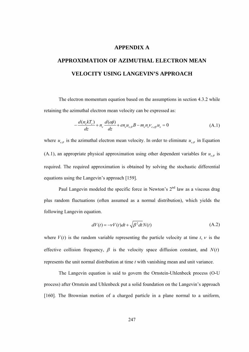
247
APPENDIX A
APPROXIMATION OF AZIMUTHAL ELECTRON MEAN
VELOCITY USING LANGEVIN’S APPROACH
The electron momentum equation based on the assumptions in section 4.3.2 while
retaining the azimuthal electron mean velocity can be expressed as:
, ,
( ) ( )0e e
e e e e e e eff e
d n kT d en en u B m n u
dz dz (A.1)
where ,eu is the azimuthal electron mean velocity. In order to eliminate ,eu in Equation
(A.1), an appropriate physical approximation using other dependent variables for ,eu is
required. The required approximation is obtained by solving the stochastic differential
equations using the Langevin’s approach [159].
Paul Langevin modeled the specific force in Newton’s 2 P
ndP law as a viscous drag
plus random fluctuations (often assumed as a normal distribution), which yields the
following Langevin equation.
2( ) ( ) ( )dV t V t dt dt N t (A.2)
where ( )V t is the random variable representing the particle velocity at time t, is the
effective collision frequency, is the velocity space diffusion constant, and ( )N t
represents the unit normal distribution at time t with vanishing mean and unit variance.
The Langevin equation is said to govern the Ornstein-Uhlenbeck process (O-U
process) after Ornstein and Uhlenbeck put a solid foundation on the Langevin’s approach
[160]. The Brownian motion of a charged particle in a plane normal to a uniform,
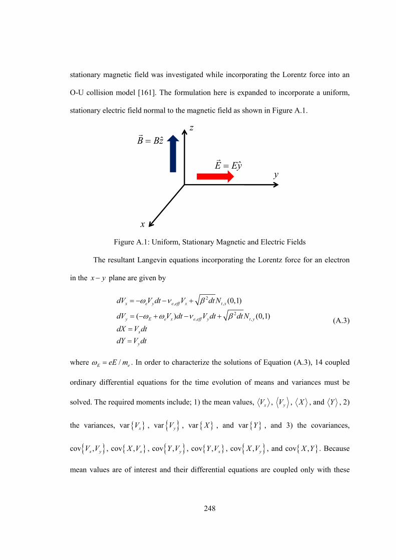
248
stationary magnetic field was investigated while incorporating the Lorentz force into an
O-U collision model [161]. The formulation here is expanded to incorporate a uniform,
stationary electric field normal to the magnetic field as shown in Figure A.1.
ˆB Bz
ˆE Ey
x
y
z
Figure A.1: Uniform, Stationary Magnetic and Electric Fields
The resultant Langevin equations incorporating the Lorentz force for an electron
in the x y plane are given by
2, ,
2, ,
(0,1)
( ) (0,1)
x e y e eff x t x
y E e x e eff y t y
x
y
dV V dt V dt N
dV V dt V dt dt N
dX V dt
dY V dt
(A.3)
where /E eeE m . In order to characterize the solutions of Equation (A.3), 14 coupled
ordinary differential equations for the time evolution of means and variances must be
solved. The required moments include; 1) the mean values, xV , yV , X , and Y , 2)
the variances, var xV , var yV , var X , and var Y , and 3) the covariances,
cov ,x yV V , cov , xX V , cov , yY V , cov , xY V , cov , yX V , and cov ,X Y . Because
mean values are of interest and their differential equations are coupled only with these
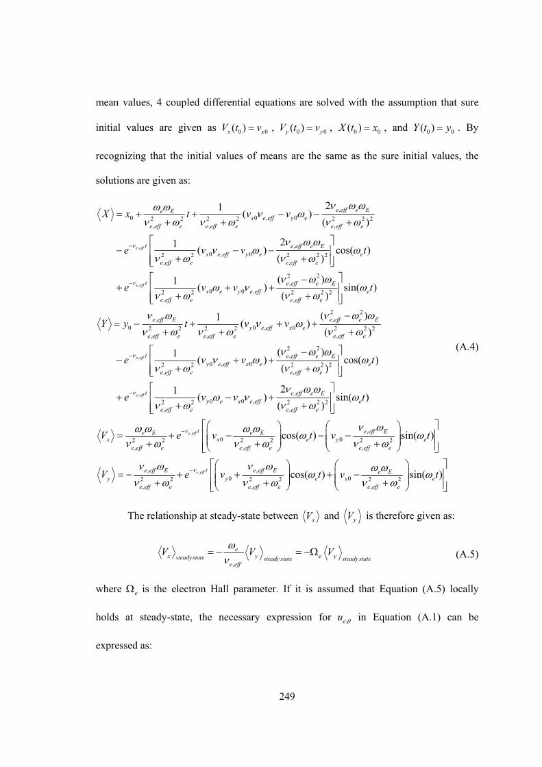
249
mean values, 4 coupled differential equations are solved with the assumption that sure
initial values are given as 0 0( )x xV t v , 0 0( )y yV t v , 0 0( )X t x , and 0 0( )Y t y . By
recognizing that the initial values of means are the same as the sure initial values, the
solutions are given as:
,
,
,0 0 , 02 2 2 2 2 2 2
, , ,
,0 , 02 2 2 2 2
, ,
0 0 ,2 2,
21( )
( )
21( ) cos( )
( )
(1( )
e eff
e eff
e eff e Ee Ex e eff y e
e eff e e eff e e eff e
t e eff e Ex e eff y e e
e eff e e eff e
tx e y e eff
e eff e
X x t v v
e v v t
e v v
,
2 2,
2 2 2,
2 2, ,
0 0 , 02 2 2 2 2 2 2, , ,
2 2,
0 , 02 2 2 2 2, ,
)sin( )
( )
( )1( )
( )
( )1( )
( )e eff
e eff e Ee
e eff e
e eff E e eff e Ey e eff x e
e eff e e eff e e eff e
t e eff e Ey e eff x e
e eff e e eff e
t
Y y t v v
e v v
,
,
,0 0 ,2 2 2 2 2
, ,
,0 02 2 2 2 2 2
, , ,
cos( )
21( ) sin( )
( )
cos( ) sin( )
e eff
e eff
e
t e eff e Ey e x e eff e
e eff e e eff e
t e eff Ee E e Ex x e y e
e eff e e eff e e eff e
t
e v v t
V e v t v t
,, ,0 02 2 2 2 2 2
, , ,
cos( ) sin( )e eff te eff E e eff E e Ey y e x e
e eff e e eff e e eff e
V e v t v t
(A.4)
The relationship at steady-state between xV and yV is therefore given as:
,
ex y e ysteady state steady state steady state
e eff
V V V
(A.5)
where e is the electron Hall parameter. If it is assumed that Equation (A.5) locally
holds at steady-state, the necessary expression for ,eu in Equation (A.1) can be
expressed as:

250
,,
ee e
e eff
u u
(A.6)
Finally, substituting Equation (A.6) into Equation (A.1) results in Equation (4.3)
in section 4.3.2.
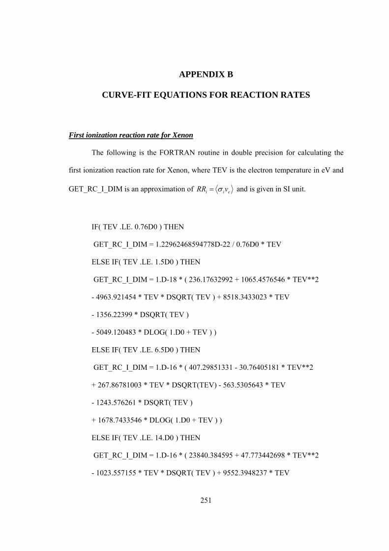
251
APPENDIX B
CURVE-FIT EQUATIONS FOR REACTION RATES
UFirst ionization reaction rate for Xenon
The following is the FORTRAN routine in double precision for calculating the
first ionization reaction rate for Xenon, where TEV is the electron temperature in eV and
GET_RC_I_DIM is an approximation of eii vRR and is given in SI unit.
IF( TEV .LE. 0.76D0 ) THEN
GET_RC_I_DIM = 1.22962468594778D-22 / 0.76D0 * TEV
ELSE IF( TEV .LE. 1.5D0 ) THEN
GET_RC_I_DIM = 1.D-18 * ( 236.17632992 + 1065.4576546 * TEV**2
- 4963.921454 * TEV * DSQRT( TEV ) + 8518.3433023 * TEV
- 1356.22399 * DSQRT( TEV )
- 5049.120483 * DLOG( 1.D0 + TEV ) )
ELSE IF( TEV .LE. 6.5D0 ) THEN
GET_RC_I_DIM = 1.D-16 * ( 407.29851331 - 30.76405181 * TEV**2
+ 267.86781003 * TEV * DSQRT(TEV) - 563.5305643 * TEV
- 1243.576261 * DSQRT( TEV )
+ 1678.7433546 * DLOG( 1.D0 + TEV ) )
ELSE IF( TEV .LE. 14.D0 ) THEN
GET_RC_I_DIM = 1.D-16 * ( 23840.384595 + 47.773442698 * TEV**2
- 1023.557155 * TEV * DSQRT( TEV ) + 9552.3948237 * TEV
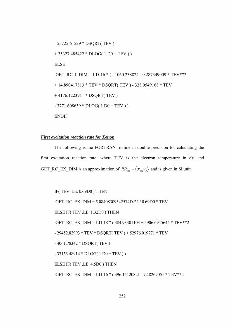
252
- 55725.61529 * DSQRT( TEV )
+ 35327.485422 * DLOG( 1.D0 + TEV ) )
ELSE
GET_RC_I_DIM = 1.D-16 * ( - 1060.238824 - 0.287349009 * TEV**2
+ 14.890417813 * TEV * DSQRT( TEV ) - 328.0549168 * TEV
+ 4176.1223911 * DSQRT( TEV )
- 3771.608639 * DLOG( 1.D0 + TEV ) )
ENDIF
UFirst excitation reaction rate for Xenon
The following is the FORTRAN routine in double precision for calculating the
first excitation reaction rate, where TEV is the electron temperature in eV and
GET_RC_EX_DIM is an approximation of eexcexc vRR and is given in SI unit.
IF( TEV .LE. 0.69D0 ) THEN
GET_RC_EX_DIM = 5.08408309542574D-22 / 0.69D0 * TEV
ELSE IF( TEV .LE. 1.32D0 ) THEN
GET_RC_EX_DIM = 1.D-18 * ( 384.93301103 + 5906.6945644 * TEV**2
- 29452.82993 * TEV * DSQRT( TEV ) + 52976.019771 * TEV
- 4061.78342 * DSQRT( TEV )
- 37153.48914 * DLOG( 1.D0 + TEV ) )
ELSE IF( TEV .LE. 4.5D0 ) THEN
GET_RC_EX_DIM = 1.D-16 * ( 396.15120821 - 72.8269051 * TEV**2
253
+ 559.35258841 * TEV * DSQRT( TEV ) - 1206.807152 * TEV
- 1251.468902 * DSQRT( TEV )
+ 2273.5013847 * DLOG( 1.D0 + TEV ) )
ELSE IF( TEV .LE. 14.D0 ) THEN
GET_RC_EX_DIM = 1.D-16 * ( - 9530.927928 - 12.8807594 * TEV**2
+ 317.4647051 * TEV * DSQRT( TEV ) - 3484.270567 * TEV
+ 24038.281055 * DSQRT( TEV )
- 16718.66551 * DLOG( 1.D0 + TEV ) )
ELSE
GET_RC_EX_DIM = 1.D-16 * ( - 1764.678691 - 0.370317143 * TEV**2
+ 14.56036509 * TEV * DSQRT( TEV ) - 228.5523671 * TEV
+ 1832.91572 * DSQRT( TEV )
- 783.6626165 * DLOG( 1.D0 + TEV ) )
ENDIF
UMomentum transfer collision reaction rate for Xenon
The following is the FORTRAN routine in double precision for calculating the
momentum transfer collision reaction rate, where TEV is the electron temperature in eV
and GET_RC_MT_DIM is an approximation of emtmt vRR and is given in SI unit.
IF( TEV .LE. 0.66D0 ) THEN
GET_RC_MT_DIM = 2.80018415651284D-021 / 0.66D0 * TEV
ELSE IF( TEV .LE. 0.96D0 ) THEN
254
GET_RC_MT_DIM = 1.D-18 * ( 1942.7833599 + 21752.481587 * TEV**2
- 106373.3163 * TEV * DSQRT( TEV ) + 189020.76071 * TEV
- 17006.19333 * DSQRT( TEV )
- 128882.7118 * DLOG( 1.D0 + TEV ) )
ELSE IF( TEV .LE. 1.5D0 ) THEN
GET_RC_MT_DIM = 1.D-16 * ( 86.367756586 + 340.94984236 * TEV**2
- 1620.465496 * TEV * DSQRT( TEV ) + 2820.6047391 * TEV
- 462.4640629 * DSQRT( TEV )
- 1680.702613 * DLOG( 1.D0 + TEV ) )
ELSE IF( TEV .LE. 14.D0 ) THEN
GET_RC_MT_DIM = 1.D-16 * ( - 4897.223675 + 23.050024721 * TEV**2
- 182.8462002 * TEV * DSQRT( TEV ) - 632.7605435 * TEV
+ 13942.419088 * DSQRT( TEV )
- 11944.35514 * DLOG( 1.D0 + TEV ) )
ELSE
GET_RC_MT_DIM = 1.D-16 * ( - 1920.569321 + 0.1200436464 * TEV**2
- 7.301695795 * TEV * DSQRT( TEV ) + 177.65021262 * TEV
- 2572.495579 * DSQRT( TEV )
+ 3848.6613267 * DLOG( 1.D0 + TEV ) )
ENDIF
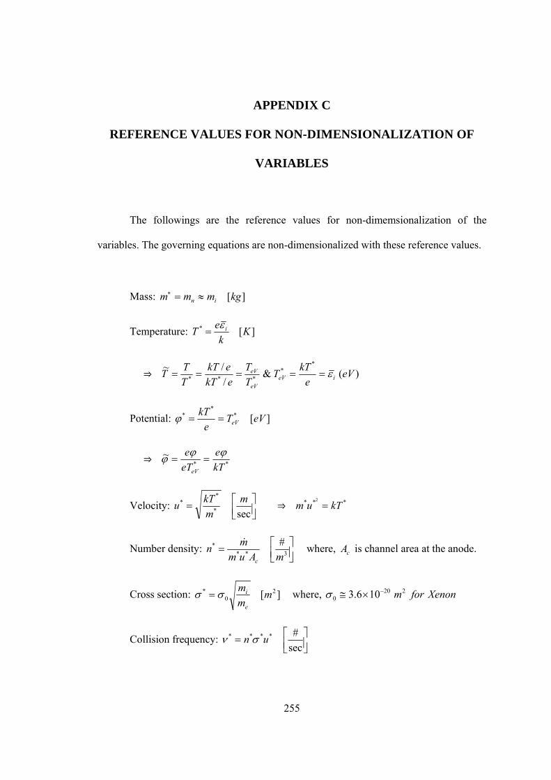
255
APPENDIX C
REFERENCE VALUES FOR NON-DIMENSIONALIZATION OF
VARIABLES
The followings are the reference values for non-dimemsionalization of the
variables. The governing equations are non-dimensionalized with these reference values.
Mass: ][kgmmm in
Temperature: ][* Kk
eT i
fl )(&/
/~ **
***eV
e
kTT
T
T
ekT
ekT
T
TT ieV
eV
eV
Potential: ][**
* eVTe
kTeV
fl **
~kT
e
eT
e
eV
Velocity:
sec*
** m
m
kTu fl *** 2
kTum
Number density:
3*** #
mAum
mn
c
where, cA is channel area at the anode.
Cross section: ][ 20
* mm
m
e
i where, Xenonform2200 106.3
Collision frequency:
sec
#**** un

256
Length: ][1
***
** m
n
ul
fl 1*** ln
Time: [sec]11
*
*
*****
u
l
unt
257
APPENDIX D
DESCRIPTION OF THE DEVELOPED TOOL: HOW-TO-USE
D.1 Introduction
The developed tool is a numerical analysis software for the typical HET
configuration. The algorithms are described in Chapter IV. The tool is coded in
FORTRAN and consists of the following components:
A main program
Readout of input variables and pre-processing
Calculation of reference variables and non-dimensionalization
Calculation of miscellaneous required variables, the Gaussian-Legengdre
abscissas and weights, and readout of the magnetic field distribution in case it is
given
Iterative solution procedure using relaxation method
Calculation of anomalous coefficients as a function of discharge voltage
Calculation of collision frequencies and reaction rates
Finite difference method for ionization/acceleration region
Post-processing for plasma structures, performance, and data for plotting
Miscellaneous routines including spline and grid clustering
D.2 Usage
To use the developed tool, execute “hall1d.exe” with a given input file in the
command window or double click the execution file in the directory.

258
D.2.1 Input
The inputs consist of a total of 13 groups as follows.
1) Group 1: propellant information (limited to Xenon)
a. AMW_DIM: molecular weight of propellant species [kg/kmole]
b. EI_DIM: threshold of first ionization energy [eV]
c. EEXCITE_DIM: first excitation energy [eV]
d. AMDOT_DIM: propellant (anode) mass flow rate [kg/s]
2) Group 2: power
a. PHI_D_DIM: discharge voltage [V]
b. COE_ANO1: inverse of the anomalous coefficient inside the channel
c. COE_ANO2: inverse of the anomalous coefficient outside the channel
3) Group 3: magnetic field information
a. BMAX_DIM: maximum radial magnetic field strength [T]
b. BCATH_DIM: radial magnetic field strength at the cathode [T]
c. COEMAG: shape coefficient of radial magnetic field strength inside the
channel
d. IMAGOPT: magnetic field option, 1 – analytic expression (no input required),
2 – given in input file (mf.dat file must exist in the same directory as the
execution file)
e. IMAGDISTOPT: When IMAGOPT = 1, option for magnetic field distribution
in the plume region, 1 – linear, 2 - quadratic
4) Group 4: geometry information
a. D_L_DIM: channel length [m]
259
b. R1_DIM: inner radius [m]
c. R2_DIM: outer radius [m]
d. Z_CATH_DIM: distance from exit plane to the cathode line [m]
5) Group 5: max constraints
a. TE_MAX0_DIM: maximum allowable electron temperature the material can
withstand [eV]
6) Group 6: boundary conditions
a. T_A_DIM: anode temperature [K]
b. TE_C_DIM: electron temperature at the cathode line [eV]
c. PHI_C_DIM: electric potential at the cathode line [V]
7) Group 7: guessed values
a. UI_C_GUESS: initial guess for ion mean velocity at the cathode line [m/s]
b. TE_M_GUESS: initial guess for electron temperature at the matching point
[eV]
c. NE_M_GUESS: initial guess for plasma number density at the matching point
[#/mP
3P]
8) Group 8: additional parameters
a. IWOPT: option for wall collision model, 1 – constant, 2 – NASA model, 3 –
Ahedo’s model
b. IMUEOPT: option for electron mobility expression, 1 – classical expression, 2
– expression with the assumption of high electron hall parameter

260
c. ANODIST: fraction of distance from the thruster exit to the cathode line for
smooth transition of the anomalous coefficient between inside and outside the
channel
d. WALDIST: fraction of distance from the thruster exit to the cathode line for
smooth transition of wall collision effect between inside and outside the
channel
9) Group 9: option for collision frequency, 0 – no inclusion, 1 – inclusion
a. IMNCOL: electron-neutral momentum exchange collision
b. IMEICOL: electron-ion Coulomb collision
c. IMWCOL: electron-wall momentum collision
d. IMBCOL: effective Bohm collision
e. IEICOL: ionization energy loss collision
f. IRECOL: recombination collision
g. IEXCOL: excitation energy loss collision
h. IEWCOL: wall energy loss collision
i. IEACOL: additional ionization energy loss collision
10) Group 10: option for grid generation
a. ICLUST: 0 – equal space, else – clustering
b. BETA: degree of clustering ( >1 ), the smaller, the more clustering
c. IPOS1: type of clustering for channel region, negative – start point clustering, 0
– both side clustering, positive – end point clustering
d. IPOS2: type of clustering for outside region with the same options as IPOS1
11) Group 11: general numerical inputs

261
a. NQ: number of dependent variables to be solved
b. M: number of grid points
c. ITMAX: maximum iteration for global iteration
d. STEP: step size for numerical differentiation
e. CONV: convergence criterion (log scale)
f. OMEGA: relaxation factor
g. NQUAD: number of points used for the Gaussian-Legengdre quadrature rule
12) Group 12: numerical inputs for finite difference ODE solver
a. CONVODE: convergence criterion
b. SLOWODE: factor for convergence rate adjustment
c. ITMAXODE: maximum iteration
13) Group 13: print option, 0 – no print, 1 – print
a. IPREF: reference variable values
b. IPMAG: radial magnetic field distribution
c. IPGRID: generated grid
d. IPINIT: initial guessed values
e. IPPERI: periodic solutions
f. IPSOL: final solutions
g. IPERR: error history
h. IPOUT: performance history
i. NSTO: iteration number interval for saving intermediate solutions
j. NERR: iteration number interval for saving error

262
k. NAVE: in case of oscillatory solution, average values during last NAVE
iterations
D.2.2 Outputs
The outputs consist of an exit mode code and a total of 8 groups as follows.
1) Exit mode code: solution case number explained in section 5.3.4
2) Group 1: constant values
a. COE_ANO1, COE_ANO2: anomalous coefficients inside and outside the
channel
b. WE_MAX, Z_WE_MAX: maximum electron gyro frequency [rad/s] and its
location [cm]
c. UN0: neutral mean velocity [m/s]
d. NN0: neutral number density at the matching point [#/mP
3P]
e. TE_C: electron temperature at the cathode [eV]
f. PHI_C: electric potential at the cathode [V]
g. EE_C: electron internal energy at the cathode [eV]
h. A: channel area [mP
2P]
3) Group 2: performance
a. ISP: anode specific impulse [s]
b. THRUST: thrust [mN]
c. CRT_D: discharge current [A]
d. PD: discharge power [kW]
4) Group 3: efficiencies
a. ETA_ANO: anode efficiency

263
b. ETA_E: electrical efficiency
c. ETA_A: acceleration efficiency
d. ETA_U: utilization efficiency
5) Group 4: matching point variables
a. Z_M: location of the matching point [cm]
b. TE_M: electron temperature at the matching point [eV]
c. ANE_M: plasma number density at the matching point [#/mP
3P]
d. PHI_M: electric potential at the matching point [V]
6) Group 5: other parameters
a. ANU_I_AVE: average ionization collision frequency in the presheath region
[#/s]
b. UE_CATHODE: electron mean velocity at the cathode line [m/s]
7) Group 6: continuity check
a. MDOT_C: total mass flow rate at the cathode line [kg/s]
b. ID_A: discharge current at the anode [A]
8) Group 7: maximum properties
a. TE_MAX, Z_TE_MAX: maximum electron temperature [eV] and its location
[cm]
b. IR_MAX, Z_IR_MAX: maximum ionization rate [#/mP
3P-s] and its location [cm]
c. EF_MAX, Z_EF_MAX: maximum electric field [V/m] and its location [cm]
d. HP_MAX, Z_HP_MAX: maximum electron Hall parameter and its location
[cm]

264
9) Group 8: 4 constraint values explained in section 6.2.3 and maximum electron
temperature constraint value for later use
265
REFERENCES
[1] Dan M. Goebel, and Ira Katz, “Fundamentals of Electric Propulsion,” JPL Space Science and Technology Series, A John Wiley & Sons, Inc., 2008.
[2] Ronald W. Humble, Gary N. Henry, and Wiley J. Larson, “Space Propulsion Analysis and Design,” Space Technology Series, The McGraw-Hill Companies, Inc., 1995.
[3] Wiley J. Larson, and James R. Wertz, “Space Mission Analysis and Design,” The Space Technology Library, Microcosm, Inc., 2004.
[4] Gulczinski, P., and Spores, R., “Analysis of Hall-effect thrusters and ion engines for orbit transfer missions,” AIAA-96-2973, 32P
ndP Joint Propulsion Conference, Lake
Buena Vista, FL. July 1-3, 1996.
[5] Marc D. Rayman, Thomas C. Fraschetti, Carol A. Raymond, and Christopher T. Russell, “Dawn: A Mission in Development for Exploration of Main Belt Asteroids Vesta and Ceres,” Acta Astronautica, Vol 58, 2006, pp. 605-616.
[6] E. Y. Choueiri, “A Critical History of Electric Propulsion: The First 50 Years (1906 – 1956)”, Journal of Propulsion and Power, Vol 20, No 2, Mar.-Apr., 2004, pp. 193-203.
[7] Richard R. Hofer, “Development and Characterization of High-Efficiency, High-Specific Impulse Xenon Hall Thrusters”, NASA/CR-2004-213099.
[8] E. H. Hall, “On a New Action of the Magnet on Electric Currents,” American Journal of Mathematics, Vol 2, 1879, pp. 287-292.
[9] Harold R. Kaufman, “Technology of Closed-Drift Thrusters,” AIAA Journal, Vol. 23, No. 1, 1983, pp. 78-87.
[10] Raymond S. Robinson, Terry D. Schemmel, and Michael J. Patterson, “Closed-Drift Thruster Investigation,” NASA CR-179497, Jun. 1986.
266
[11] Edgar Y. Choueiri, “Fundamental Difference between the Two Variants of Hall Thrusters: SPT and TAL”, AIAA-2001-3504, 37P
thP AIAA Joint Propulsion
Conference, Salt Lake City, UT, July 9-11, 2001.
[12] Michelle R. Kirby, “A Methodology for Technology Identification, Evaluation, and Selection in Conceptual and Preliminary Aircraft Design,” Ph.D. Thesis, Georgia Institute of Technology, Mar. 2001.
[13] Mavris, D. N., Kirby, M. R., and Qiu, S., “Technology Impact Forecasting for a High Speed Civil Transport,” SAE-985547, World Aviation Conference, Sept. 1998, Anaheim, CA.
[14] Mankins, John C., “Technology Readiness Levels: A White Paper,” NASA, Office of Space Access and Technology, Advanced Concepts Office, 1995.
[15] Charles E. Garner, James E. Polk, Lewis C. Pless, Keith D. Goodfellow, and John R. Brophy, “Performance Evaluation and Life Testing of the SPT-100,” IEPC-93-091, 23P
rdP International Electric Propulsion Conference, Sept. 1993, Seattle, WA, USA.
[16] John M. Sankovic, John A. Hamley, and Thomas W. Haag, “Performance Evaluation of the Russian SPT-100 Thruster at NASA LeRC,” IEPC-93-094, 23 P
rdP
International Electric Propulsion Conference, Sept. 1993, Seattle, WA, USA.
[17] Arhipov B. A., Krochak L. Z., Kudriavcev S. S., Murashko V. M., and Randolph T., “Investigation of the Stationary Plasma Thruster (SPT-100) Characteristics and Thermal Maps at the Raised Discharge Power,” AIAA-98-3791, 1998.
[18] N. Gascon, M. Dudeck, and S. Barral, “Wall Material Effects in Stationary Plasma Thrusters. I. Parametric Studies of an SPT-100,” Physics of Plasmas, Vol. 10, No. 10, Oct. 2003.
[19] E. E. Barkalov, A. N. Veselovzorov, A. A. Pogorelov, E. B. Svirskii, and V. A. Smirnov, “Composition of the Beam of an SPT-100 Stationary Plasma Thruster,” Instruments and Experimental Techniques, Vol. 51, No. 2, 2008, pp. 263-267.
[20] Maslenikov, N. A., Russian Electric Propulsion Seminar, Massachusetts Institute of Technology, 1991.

267
[21] Haas, J. M., Gulczinski, F. S., Gallimore, A. D, Spanjers, G. G., and Spores, R. A., “Performance Characteristics of a 5kW Laboratory Hall Thruster,” AIAA-98-3503, 34P
thP Joint Propulsion Conference, Cleveland, OH, July 1998.
[22] Frank Stanley Gulczinski III, "Examination of the Structure and Evolution of Ion Energy Properties of a 5kW Class Laboratory Hall Effect Thruster at Various Operational Conditions," Ph. D. Dissertation, School of Aerospace Engineering, The University of Michigan, Ann Arbor, MI, 1999.
[23] Brophy, J. R., “Ion Thruster Performance Model,” NASA CR-174810, Dec. 1984.
[24] Leonard Biagioni, Massimo Saverdi, and Mariano Andrenucci, “Scaling and Performance Prediction of Hall Effect Thrusters,” AIAA 2003-4727, 39P
thP
AIAA/ASME/SAE/ASEE Joint Propulsion Conference and Exhibit, 20-23 July 2003, Huntsville, Alabama.
[25] Hofer, R. R., and Jankovsky, R. S., “A Hall Thruster performance Model Incorporating the Effects of a Multiply-Charged Plasma,” AIAA 2001-3322, 37P
thP
AIAA/ASME/SAE/ASEE Joint Propulsion Conference and Exhibit, Salt Lake city UT, July 2001.
[26] Khayms, V., and Martinez-Sanchez, M., “Design of a Miniaturized Hall Thruster for Microsatellites,” AIAA 1996-3291, 32 P
ndP AIAA/ASME/SAE/ASEE Joint Propulsion
Conference and Exhibit, Lake Buena Vista, FL, July 1-3, 1996.
[27] Yu Daren, Ding Yongjie, and Zeng Zhi, “Improvement on the Scaling Theory of the Stationary Plasma Thruster,” Journal of Propulsion and Power, Vol. 21, No. 1., 2005.
[28] Marc D. Rayman, Pamela A. Chadbourne, Jeffery S. Culwell, and Steven N. Williams, “Mission Design for Deep Space 1: A Low-Thrust Technology Validation Mission,” Acta Astronautica, Vol. 45, Nos. 4-9, 1999, pp. 381-388.
[29] Marc D. Rayman, Philip Varghese, David H. Lehman, and Leslie L. Livesay, “Results from the Deep Space 1 Technology Validation Mission,” Acta Astronautica, Vol. 47, Nos. 2-9, 2000, pp. 475-487.
[30] Racca, G. D., Foing, B. H. and Coradini, M., “SMART-1: The First Time of Europe to the Moon,” Earth, Moon and Planets, Vol. 85, 2001.
268
[31] Giuseppe D. Racca, “New Challenges to Trajectory Design by the Use of Electric Propulsion and Other New Means of Wandering in the Solar System,” Celestial Mechanics and Dynamical Astronomy, Vol. 85, 2003, pp. 1-24.
[32] Kristina Alemany, and Robert D. Braun, “Survey of Global Optimization Methods for Low-Thrust, Multiple Asteroid Tour Missions,” AAS 07-211.
[33] Damon Landau, Theresa Kowalkowski, Jon Sims, Thomas Randolph, and Paul Timmerman, “Electric Propulsion System Selection Process for Interplanetary Missions,” AIAA/AAS Astrodynamics Specialist Conference and Exhibit, 18-21 Aug. 2008, Honolulu, Hawaii.
[34] C. A. Kluever, “Geostationary Orbit Transfers Using Solar Electric Propulsion with Specific Impulse Modulation,” Journal of Spacecraft and Rockets, Vol. 41, No. 3, 2004, pp. 461-466.
[35] Giovanni Mengali, and Alessandro A. Quarta, “Fuel-Optimal, Power-Limited Rendezvous with Variable Thruster Efficiency,” Journal of Guidance, Control, and Dynamics, Vol. 28, No. 6, 2005, pp. 1194-1199.
[36] David Manzella, David Oh, and Randall Aadland, “Hall Thruster Technology for NASA Science Missions,” AIAA-2005-3675, 41 P
stP AIAA/ASME/SAE/ASEE Joint
Propulsion Conference & Exhibit, 10-13 July, 2005, Tucson, Arizona.
[37] Bucovsky Adrian Eyer, Jesse and Mavris, Dimitri, “Design Space Exploration for Boom Mitigation on a Quiet Supersonic Business Jet,” AIAA 3P
rdP Annual Aviation
Technology, Integration, and Operation (ATIO) Technology Conference, Denver, Co, Nov. 2003.
[38] Frits, Andrew P. and Mavris, Dimitri N., “A Screening Method for Customizing Designs around Non-Convergent Regions of Design Spaces,” 9P
thP AIAA/ISSMO
Symposium and Exhibit on Multidisciplinary Analysis and Optimization, Atlanta, GA, Sept. 2002.
[39] Frits, Andrew P., Mavris, N. Dimitri, Kusmik Aldo, and Krol Jr. William, “Examination of a Torpedo Performance Space and its Relation to the System Design Space,” 9 P
thP AIAA/ISSMO Symposium and Exhibit on Multidisciplinary
Analysis and Optimization, Atlanta, GA, Sept. 2002.
269
[40] Walter G. Vincenti, and Charles H. Kruger, Jr., “Introduction to Physical Gas Dynamics,” John Wiley & Sons, Inc., 1965.
[41] Francis F. Chen, “Introduction to Plasma Physics and Controlled Fusion,” Plenum Press, NY, 1984.
[42] J. A. Bittencourt, “Fundamentals of Plasma Physics,” Springer-Verlag New York, Inc., 2004.
[43] Edward M. Purcell, “Electricity and Magnetism,” McGraw-Hill Book Company, 2P
ndP
Ed., 1985.
[44] William H. Hayt, Jr., and John A. Buck, “Engineering Electromagnetics,” McGraw-Hill Book Company, 7 P
thP Ed., 2006.
[45] G. A. Bird, “Molecular Gas dynamics and the Direct Simulation of Gas Flows,” Oxford University Press Inc., New York, 1994.
[46] Weston M. Stacey, Jr., “FUSION: An Introduction to the Physics and Technology of Magnetic Confinement Fusion,” John Wiley & Sons, Inc., 1984.
[47] Iain D. Boyd, “Numerical Modeling of Spacecraft Electric Propulsion Thrusters,” Progress in Aerospace Sciences, Vol. 41, 2005, pp. 669-687.
[48] C. K. Birdsall, and A. B. Landon, “Plasma Physics via Computer Simulation,” Taylor & Francis Group, New York, 2005.
[49] R. W. Hockney, and J. W. Eastwood, “Computer Simulation using Particles,” Taylor & Francis Group, New York, 1988.
[50] J. P. Boeuf, and E. Marode, “A Monte Carlo Analysis of an Electron Swarm in a Non-Uniform Field: the Cathode Region of a Glow Discharge in Helium,” Journal of Physics D: Applied Physics, Vol. 15, 1982, pp. 2169-2187.
[51] Nicholas Metropolis, Arianna W. Rosenbluth, Marshall N. Rosenbluth, and Augusta H. Teller, “Equation of State Calculations by Fast Computing Machines,” The Journal of Chemical Physics, Vol. 21, No. 6, 1953, pp. 1087-1092.
270
[52] James Joseph Szabo, Jr., “Fully Kinetic Numerical Modeling of a Plasma Thruster,” Ph.D. Thesis, Massachusetts Institute of Technology, Feb. 2001.
[53] Christopher A. Lentz, “Transient One Dimensional Numerical Simulation of Hall Thrusters,” Master Thesis, Massachusetts Institute of Technology, Sept. 1993.
[54] K-U Riemann, “The Bohm Criterion and Sheath Formation,” Journal of Physics D: Applied Physics, Vol. 24, 1991, pp. 493-518.
[55] S. A. Self, “Exact Solution of the Collisionless Plasma-Sheath Equation,” The Physics of Fluids, Vol. 6, No. 12, Dec. 1963, pp. 1762-1768.
[56] Seungwon Lee, Paul von Allmen, Wolfgang Fink, Anastassios E. Petropoulos, and Richard J. Terrile, “Design and Optimization of Low-thrust Orbit Transfer,” IEEEAC paper #2.1204, 2005.
[57] Arthur E. Bryson, Jr., Yu-Chi Ho, “Applied Optimal Control,” Taylor & Francis Group, LLC, Revised Edition, 1975.
[58] Frank L. Lewis, “Applied Optimal Control and Estimation,” Prentice Hall, 1992.
[59] Lorenzo Casalino, Guido Colasurdo, and Matteo Rosa Sentinella, “Indirect Optimization Method for Low-Thrust Interplanetary Trajectories,” IEPC-2007-356, 30P
thP International Electric Propulsion Conference, Sept. 17-20, 2007, Florence, Italy.
[60] Christopher L. Ranieri, and Cesar A. Ocampo, “Optimization of Roundtrip, Tim-Constraintd, Finite Burn Trajectories via an Indirect Method,” Journal of Guidance, Control, and Dynamics, Vol. 28, No. 2, 2005, pp. 306-314.
[61] Sean Tang, and Bruce A. Conway, “Optimization of Low-Thrust Interplanetary Trajectories Using Collocation and Nonlinear Programming,” Journal of Guidance, Control, and Dynamics, Vol. 18, No. 3, 1995, pp. 599-604.
[62] Matthew A. Vavrina, and Kathleen C. Howell, “Global Low-Thrust Trajectory Optimization through Hybridization of a Genetic Algorithm and a Direct Method,” AAS/AIAA Astrodynamics Specialists Conference, Aug. 2008, Honolulu, Hawaii.
271
[63] Lantoine, G., “A Methodology for Robust Optimization of Low-Thrust Trajectories in Multi-Body Environments,” Ph.D. Thesis, Georgia Institute of Technology, 2010 (in completion).
[64] V. Latocha, L. Garrigues, P. Degond, and J. P. Boeuf, “Numerical Simulation of Electron Transport in the Channel Region of a Stationary Plasma Thruster,” Plasma Sources Science and Technology, Vol. 11, 2002, pp. 104-114.
[65] J. C. Adam, A. Heron, and G. Laval, “Study of Stationary Plasma Thrusters Using Two-Dimensional Fully Kinetic Simulations,” Physics of Plasmas, Vol. 11, No. 1, Jan. 2004, pp. 295-305.
[66] Francesco Taccogna, Savino Longo, Mario Capitelli, and Ralf Schneider, “Plasma Flow in a Hall Thruster,” Physics of Plasmas, Vol. 12, 043502, 2005.
[67] F. Taccogna, S. Longo, M. Capitelli, and R. Schneider, “Start-Up Transient in a Hall Thruster,” Contributions to Plasma Physics, Vol. 46, No. 10, 2006, pp. 781-786.
[68] John Michael Fife, “Two-Dimensional Hybrid Particle-In-Cell Modeling of Hall Thrusters,” Master Thesis, Massachusetts Institute of Technology, May 1995.
[69] John Michael Fife, “Hybrid-PIC Modeling and Electrostatic Probe Survey of Hall Thruster,” Ph.D. Thesis, Massachusetts Institute of Technology, Sept. 1998.
[70] Justin W. Koo, and Iain D. Boyd, “Computational Modeling of Stationary Plasma Thrusters,” AIAA-2003-10113, 39 P
thP AIAA/ASME/SAE/ASEE Joint Propulsion
Conference, Huntsville, AL, July 2003.
[71] Michelle K. Scharfe, Nicolas Gascon, Mark A. Cappelli, and Eduardo Fernandez, “Comparison of Hybrid Hall Thruster Model to Experimental Measurements,” Physics of Plasmas, Vol. 13, 083505, 2005.
[72] G. Hagelaar, J. Bareilles, L. Garrigues, and J. P. Boeuf, “Two Dimensional Model of a Stationary Plasma Thruster,” Journal of Applied Physics, Vol. 91, 2002, pp. 5592-5598.
[73] E. Ahedo, P. Martinez, and M. Martinez-Sanchez, “Steady and Linearly-Unsteady Analysis of a Hall Thruster with and Internal Sonic Point,” AIAA-2000-3655, 36 P
thP
272
AIAA/ASME/SAE/ASEE Joint Propulsion Conference & Exhibit, July 2000, Huntsville, Alabama.
[74] E. Ahedo, P. Martinez Cerezo, and M. Martinez-Sanchez, “1-D Performance Analysis of a Hall Thruster,” Proceedings of 3P
rdP International Conference on
Spacecraft Propulsion, Cannes, Oct. 2003.
[75] E. Ahedo, P. Martinez Cerezo, and M. Martinez-Sanchez, “One-Dimensional Model of the Plasma Flow in a Hall Thruster,” Physics of Plasmas, Vol. 8, No. 6, June 2001, pp. 3058-3068.
[76] E. Ahedo, J. M. Gallardo, and M. Martinez-Sanchez, “Effects of the Dielectric Walls on the Axial Discharge of a Hall Thruster,” AIAA-2002-4244, 38P
thP
/ASME/SAE/ASEE Joint Propulsion Conference & Exhibit, July 2002, Indianapolis, Indiana.
[77] E. Ahedo, J. M. Gallardo, and M. Martinez-Sanchez, “Model of the Plasma Discharge in a Hall Thruster with Heat Conduction,” Physics of Plasmas, Vol. 9, No. 9, Sept. 2002, pp. 4061-4070.
[78] E. Ahedo, J. M. Gallardo, and M. Martinez-Sanchez, “Effects of the Radial Plasma-Wall Interaction on the Hall Thruster Discharge,” Physics of Plasmas, Vol. 10, No. 8, Aug. 2003, pp. 3397-3409.
[79] Subrata Roy, and B. P. Pandey, “Numerical Investigation of a Hall Thruster Plasma,” Physics of Plasmas, Vol. 9, No. 9, Sept. 2002, pp. 4052-4060.
[80] Avi Cohen-Zur, Amnon Fruchtman, Joseph Ashkenazy, and Alon Gany, “Analysis of the Steady-State Axial Flow in the Hall Thruster,” Physics of Plasmas, Vol. 9, No. 10, Oct. 2002, pp. 4363-4374.
[81] J. Ashkenazy, A. Fruchtman, Y. Raitses, and N. J. Fisch, “Modeling the Behaviour of a Hall Current Plasma Accelerator,” Plasma Physics and Controlled Fusion, Vol. 41, 1999, pp. A357-A364.
[82] A. Fruchtman, N. J. Fisch, and Y. Raitses, “Hall Thruster with Absorbing Electrodes,” AIAA 2000-3659, 36P
thP AIAA/ASME/SAE/ASEE Joint Propulsion
Conference, 17-19 July 2000, Huntsville, AL.
273
[83] L. Dorf, and V. Semenov, “Anode Sheath in Hall Thrusters,” Applied Physics Letters, Vol. 83, No. 13, Sept. 2003, pp. 2551-2553.
[84] J. P. Boeuf, L. Garrigues, and L. C. Pitchford, “Modeling of a Magnetized Plasma: The Stationary Plasma Thruster,” Electron Kinetics and Application of Glow Discharge, 1998, pp. 85-100.
[85] J. P. Boeuf, and L. Garrigues, “Low Frequency Oscillations in a Stationary Plasma Thruster,” Journal of Applied Physics, Vol. 84, No. 7, Oct. 1998, pp. 3541-3554.
[86] K. Komurasaki, and Y. Arakawa, “Two-Dimensional Numerical Model of Plasma Flow in a Hall Thruster,” Journal of Propulsion and Power, Vol. 11, No. 6, 1995, pp. 1317-1323.
[87] M. Keidar, and I. D. Boyd, “Plasma Flow and Plasma-Wall Transition in Hall Thruster Channel,” Physics of Plasmas, Vol. 8, No. 12, Dec. 2001, pp. 5315-5322.
[88] H. De Sterck, “Critical Point Analysis of Transonic Flow Profiles with Heat Conduction,” SIAM Journal of Applied Dynamical Systems, Vol. 6, No. 3, pp. 645-662.
[89] D. D. Morrison, J. D. Riley, and J. F. Zancanaro, “Multiple Shooting Method for Two-Point Boundary Value Problems,” Communications of the ACM, Vol. 5, No. 12, 1962, pp. 613-614.
[90] W. H. Press, S. A. Teukolsky, W. T. Vetterling, and B. P. Flannery, “Numerical Recipes in FORTRAN,” Cambridge University Press, 1992, pp. 745-778.
[91] Laura A. Ledsinger, and John R. Olds, “Multidisciplinary Design Optimization Techniques for Branching Trajectories,” AIAA-1998-4713, 7 P
thP
AIAA/USAF/NASA/ISSMO Symposium on Multidisciplinary Analysis and Optimization, St. Louis, MO, Sept. 1998.
[92] Leonid A. Dorf, Yevgeny F. Raitses, Artem N. Smirnov, and Nathaniel J. Fisch, “Anode Fall Formation in a Hall Thruster,” AIAA-2004-3779, 40P
thP
AIAA/ASME/SAE/ASEE Joint Propulsion Conference & Exhibit, Jul. 2004, Fort Lauderdale, FL.
274
[93] L. Dorf, Y. Raitses, N. J. Fisch, and V. Semenov, “Effect of Anode Dielectric Coating on Hall Thruster Operation,” Applied Physics Letters, Vol. 84, No. 7, Feb. 2004, pp. 1070-1072.
[94] L. Dorf, Y. Raitses, and N. J. Fisch, “Experimental Studies of Anode Sheath Phenomena in a Hall Thruster Discharge,” Journal of Applied Physics, Vol. 97, 103309, 2005.
[95] V. V. Zhurin, H. R. Kaufman, and R. S. Robinson, “Physics of Closed Drift Thrusters,” Plasma Sources Science and Technology, Vol. 8, 1999, pp. R1-R20.
[96] A. M. Bishaev, and V. Kim, “Local Plasma Properties in a Hall-Current Accelerator with an Extended Acceleration Zone,” Soviet Physics – Technical Physics, Vol. 23, No. 9, Sept. 1978, pp. 1055-1057.
[97] Vladimir Kim, “Main Physical Features and Processes Determining the Performance of Stationary Plasma Thrusters,” Journal of Propulsion and Power, Vol. 14, No. 5, 1998, pp. 736-743.
[98] E. Ahedo, and J. Rus, “Vanishing of the Negative Anode Sheath in a Hall Thruster,” Journal of Applied Physics, Vol. 98, 043306, 2005.
[99] L. Dorf, V. Semenov, Y. Raitses, and N. J. Fisch, “Hall Thruster Modeling with a Given Temperature Profile,” 38 P
thP AIAA/ASME/SAE/ASEE Joint Propulsion
Conference & Exhibit, Jul. 2002, Indianapolis, Indiana.
[100] A. Morozov, Y. Esipchuk, G. Tilinin, A. Trofimov, Y. Sharov, and G. Y. Shchepkin, “Plasma Accelerator with Closed Electron Drift and Extended Acceleration Zone,” Soviet Physics – Technical Physics, Vol. 17, No. 1, 1972, pp. 38-45.
[101] A. I. Morozov, and V. V. Savelyev, Reviews of Plasma Physics, Vol. 21, Kluwer Academic/Plenum Publishers, New York, 2000, pp. 277-299.
[102] G. Janes, and R. Lowder, “Anomalous Electron Diffusion and Ion Acceleration in a Low-Density Plasma,”, The Physics of Fluids, Vol. 9, No. 6, 1966, pp. 1115-1123.
275
[103] E. Choueiri, “Plasma Oscillations in Hall Thrusters,” Physics of Plasmas, Vol. 8, No. 4, 2001, pp. 1411-1426.
[104] J. M. Gallardo, and E. Ahedo, “On the Anomalous Diffusion Mechanism in Hall-Effect Thrusters,” IEPC-2005-117, 29P
thP International Electric Propulsion
Conference, Princeton University, 2005.
[105] Hofer, R. R., Katz, I. Mikellides, I. G., and Gamero-Castano, M., “Heavy Particle Velocity and Electron Mobility Modeling in Hybrid-PIC Hall Thruster Simulations,” AIAA 2006-4658, 42th AIAA/ASME/SAE/ASEE Joint Propulsion Conference, Jul. 2004, Ft. Lauderdale, FL.
[106] Justin W. Koo, and Iain D. Boyd, “Computational Model of a Hall Thruster,” Computer Physics Communications, Vol. 164, 2004, pp. 442-447.
[107] C. Boniface, L. Garrigues, G. J. M. Hagelaar, J. P. Boeuf, D. Gawron, and S. Mazouffre, “Anomalous Cross Field Electron Transport in a Hall Effect Thruster,” Applied Physics Letters, Vol. 89, 161503, 2006.
[108] Luke Uribarri, and E. Y. Choueiri, “The Onset of Voltage Hash and its Relationship to Anode Spots in Magnetoplasmadynamic Thrusters,” IEPC-2005-084, 29P
thP International Electric Propulsion Conference, Princeton University, Oct.
2005.
[109] Luke Uribarri, “An Electron-Attracting Anode Sheath,” Documentation for Onset in MPD Thrusters, 5Thttp://www.princeton.edu/~uribarri/research/Onset/anode-sheath. pdf5T , 2006.
[110] M. Mitchner, and Charles H. Kruger, Jr., “Partially Ionized Gases,” John Wiley & Sons, Inc., New York, 1973, pp. 140.
[111] G. S. Kino, and E. K. Shaw, “Two-Dimensional Low-Pressure Discharge Theory,” The Physics of Fluids, Vol. 9, No. 3, Mar. 1966, pp. 587-593.
[112] Kimiya Komurasaki, Miharu Hirakawa, and Yoshihiro Arakawa, “Plasma Acceleration Process in a Hall-Current Thruster,” IEPC-1991-078, 22P
ndP
International Electric Propulsion Conference, Viareggio, Italy, Oct. 1991.
276
[113] Makoto Hayashi, “Determination of Electron-Xenon Total Excitation Cross-Sections, from Threshold to 100 eV, from Experimental Values of Townsend’s a,” Journal of Physics D: Applied Physics, Vol. 16, 1983, pp. 581-589.
[114] Rapp, D., and P. Englander-Golden, “Total Cross Sections for Ionization and Attachment in Gases by Electron Impact. I. Positive Ionization,” Journal of Chemical Physics, Vol. 43. No. 5, 1965.
[115] Syage, J. A., “Electron-Impact Cross Sections for Multiple Ionization of Kr and Xe,” Physical Review A, Vol. 46, No. 9, 1992.
[116] M. Suzuki, T. Taniguchi, N. Yoshimura, and H. Tagashira, “Momentum Transfer Cross Section of Xenon Deduced from Electron Drift Velocity Data,” Journal of Physics D: Applied Physics, Vol. 25, 1992, pp. 50-56.
[117] Ramsauer, C., “Ueber den Wirkungsquerschnitt der Gasmolekuele langsamen Elektronen. II. Fortsetzung and Schluss - Effective cross section of gas molecules for slow electrons. II. Continuation and final,” Ann. d. Physik - Annals of Physics, 72:345, 1923.
[118] Ramsauer, C., and R. Kollath, “Ueber den Wirkungsquerschnitt der Edelgasmolekuele gegenueber Elektronen unterhalb 1 Volt - Effective cross section of inert gas molecules against electrons below 1 volt,” Ann. d. Physik, 3:536, 1929.
[119] I. G. Mikellides, I. Katz, M. J. Mandell, and J. Steven Snyder, “A 1-D Model of the Hall Effect Thruster with an Exhaust Region,” AIAA-2001-3505, 37P
thP
AIAA/ASME/SAE/ASEE Joint Propulsion Conference and Exhibit, July 2001, Salt Lake City, Utah.
[120] 5Thttp://www.astronautix.com/engines/spt100.htm5T
[121] Justin W. Koo, and Iain D. Boyd, “Modeling of Anomalous Electron Mobility in Hall Thrusters,” Physics of Plasmas, Vol. 13, 033501, 2006.
[122] Steven R. Oleson, and Roger M. Myers, “Launch Vehicle and Power Level Impacts on Electric GEO Insertion,” AIAA-1996-2978, 32P
ndP
AIAA/ASME/SAE/ASEE Joint Propulsion Conference and Exhibit, July 1996, Lake Buena Vista, FL.
277
[123] Lee S. Mason, Robert S. Jankovsky, and David H. Manzella, “1000 Hours of Testing on a 10 Kilowatt Hall Effect Thruster,” AIAA-2001-3773, 37P
thP
AIAA/ASME/SAE/ASEE Joint Propulsion Conference and Exhibit, July 2001, Salt Lake City, Utah.
[124] Robert S. Jankovsky, and Chris McLean, “Preliminary Evaluation of a 10 kW Hall Thruster,” AIAA-99-0456, 37 P
thP AIAA Aerospace Sciences Meeting and Exhibit,
January 1999, Reno, NV.
[125] JMP® 8.0 Help File, SAS Institute Inc., 2008.
[126] K. Sankaran, L. Cassady, A.D. Kodys, and E. Y. Choueiri, “A Survey of Propulsion Options for Cargo and Piloted Missions to Mars,” The Annals of the New York Academy of Science, Vol. 1017, 2004, pp. 450-467.
[127] David T. Jacobson, David H. Manzella, Richard R. Hofer, and Peter Y. Peterson, “NASA’s 2004 Hall Thruster Program,” AIAA-2004-3600, 40 P
thP
AIAA/ASME/SAE/ASEE Joint Propulsion Conference and Exhibit, 11-14 July 2004, Fort Lauderdale, FL.
[128] David Manzella, Robert Jankovsky, and Richard Hofer, “Laboratory Model 50 kW Hall Thruster,” AIAA-2002-3676, 38P
thP AIAA/ASME/SAE/ASEE Joint Propulsion
Conference and Exhibit, 7-10 July 2002, Indianapolis, IN.
[129] C. F. Jeff Wu and Michael Hamada, “Experiment: Planning, Analysis, and Parameter Design Optimization,” Wiley-Interscience, ISBN-10 0471255114, 2000.
[130] 5Thttp://image.absoluteastronomy.com/images/encyclopediaimages/r/ru/russian_stationary_plasma_thrusters.jpg as of 05/08/20105T
[131] Danel A. Lichtin, “An Overview of Electric Propulsion Activities in US Industry – 2005,” AIAA-2005-3532, 41P
stP AIAA/ASME/SAE/ASEE Joint Propulsion
Conference & Exhibit, 10-13 July 2005, Tucson, Arizona.
[132] David J. Pidgeon, Ronald L. Corey, Birgit Sauer, and Michael L. Day, “Two Years On-Orbit Performance of SPT-100 Electric Propulsion,” AIAA-2006-5353, 24 P
thP
AIAA International Communications Satellite Conference (ICSSC) and 4t, 11-14 June 2006, San Diego, California.
278
[133] D. Milligan, D. Gestal, O. Camino, D. Estublier, and C. Koppel, “SMART-1 Electric Propulsion Operations,” AIAA-2004-3436, 40 P
thP AIAA/ASME/SAE/
ASEE Joint Propulsion Conference and Exhibit, 11-14 July 2004, Fort Lauderdale, Florida.
[134] Jack Fisher, Alfred Wilson, David King, Steve Meyer, Carl EngelBrecht, Kristi de Grys, and Lance Werthman, “The Development and Qualification of a 4.5 kW Hall Thruster Propulsion System for GEO Satellite Applications,” IEPC-01-010, 27P
thP
International Electric Propulsion Conference, 15-19 Oct. 2001, Pasadena, California.
[135] Guoqiang Zhang, B. Eddy Patuwo, and Michael Y. Hu, “Forecasting with Artificial Neural Networks: The State of the Art,” International Journal of Forecasting, Vol. 14, 1998, pp. 35-62.
[136] Debora D. Daberkow, and Dimitri N. Mavris, “New Approaches to Conceptual and Preliminary Aircraft Design: A Comparative Assessment of a Neural Network Formulation and a Response Surface Methodology,” AIAA-98-5509, World Aviation Conference, Sept. 28-30, 1998, Anaheim, CA.
[137] Carl Johnson, and Jeff Schutte, “Basic Regression Analysis for Integrated Neural Networks (BRAINN) Documentation,” Users Manual, Version 2.3, Aerospace System Design Laboratory, Georgia Institute of Technology, 2009.
[138] Leo Breiman, Jerome Friedman, Charles J. Stone, and R. A. Olshen, “Classification and Regression Trees,” Chapman and Hall/CRC Press, 1998.
[139] V. Vapnik, “The Nature of Statistical Learning Theory,” Springer, New York, 1995.
[140] Steve R. Gunn, “Support Vector Machines for Classification and Regression,” ISIS Technical Report, 1998.
[141] C. J. C. Burges, “A Tutorial on Support Vector Machines for Pattern Recognition,” Data Mining and Knowledge Discovery, Vol. 2, 1998, pp. 121-167.
[142] Ovidiu Ivanciuc, “Applications of Support Vector Machines in Chemistry,” Reviews in Computational Chemistry, Vol. 23, 2007, pp. 291-400.

279
[143] Raymond J. Mooney, “Support Vector Machines,” Lecture Note, CS391L Machine Learning, Department of Computer Science, University of Texas at Austin, 2007.
[144] Gordon R. Woodcock, and John Dankanich, “Application of Solar-Electric Propulsion to Robotic Missions in Near-Earth Space,” CP880, Space Technology and Applications International Forum – STAIF 2007, Albuquerque, NM.
[145] Gopinath, N. S., and Srinivasamuthy, K. N., “Optimal Low Thrust Orbit Transfer from GTO to Geosynchronous Orbit and Stationkeeping using Electric Propulsion System,” IAC-03-A.7.03, 54P
thP International Astronautical Congress of the
International Astronautical Federation, the International Academy of Astronautics, and the International Institute of Space Law, Bremen, Germany, Sep. 29 – Oct. 3, 2003.
[146] John W. Dankanich, and Gordon R. Woodcock, “Electric Propulsion Performance from Geo-transfer to Geosynchronous Orbits,” IEPC-2007-287, 30 P
thP International
Electric Propulsion Conference, Sep. 17-20, 2007, Florence, Italy.
[147] Yang Gao, “Linear Feedback Guidance for Low-Thrust Many-Revolution Earth-Orbit Transfers,” Journal of Spacecraft and Rockets, Vol. 46, No. 6, 2009, pp. 1320-1325.
[148] C. A. Kluever, “Geostationary Orbit Transfers Using Solar Electric Propulsion with Specific Impulse Modulation,” Journal of Spacecraft and Rockets, Vol. 41, No. 3, 2004, pp. 461-466.
[149] Sophie Geffroy and Richard Epenoy, “Optimal Low-Thrust Transfers with Constraints – Generalization of Averaging Techniques,” Acta Astronautica, Vol. 4, No.3, 1997, pp. 133-149.
[150] David Y. Oh, “Analytic Optimization of Mixed Chemical-Electric Orbit Raising Missions,” IEPC-01-173, 27 P
thP International Electric Propulsion Conference, Oct.
15-19, 2001, Pasadena, CA.
[151] Thomas M. Randolph, and David Y. Oh, “Economic Benefit Analysis of Chemical-Electric Orbit Raising Missions,” AIAA-2002-1980, 20 P
thP AIAA
International Communication Satellite Systems Conference and Exhibit, May 12-15, 2002, Montreal, Quebec, Canada.
280
[152] David Oh, Thomas Randolph, Manuel Martinez-Sanchez and Scott Kimbrel, “End to End Optimization of Two Dimensional Chemical-Electric Orbit Raising Missions,” AIAA-2002-3966, 38P
thP AIAA/ASME/SAE/ASEE Joint Propulsion
Conference and Exhibit, July 7-10, 2002, Indianapolis, Indiana.
[153] Sea Launch Company, L.L.C., “Sea Launch User’s Guide,” One World Trade Center, Suite 950, Long Beach, CA, 2008.
[154] Lantoine, G., and Russell, R. P., “A Hybrid Differential Dynamic Programming Algorithm for Robust Low-Thrust Optimization,” AIAA-2008-6615, AAS/AIAA Astrodynamics Specialist Conference and Exhibit, Aug. 2008, Honolulu, HI.
[155] Gill, P.E., Murray, W., and Saunders, M. A., “SNOPT: An SQP Algorithm for Large-Scale Constrained Optimization,” SIAM Journal on Optimization, Vol.12, No. 4, 2002, pp. 979-1006.
[156] Martins, J. R., Kroo, I. M., and Alonso, J. J., “An Automated Method for Sensitivity Analysis Using Complex Variables,” AIAA-2000-0689, 38P
thP Aerospace
Sciences Meeting, Jan. 2000, Reno, NV.
[157] Sims, J. A., and Flanagan, S. N., “Preliminary Design of Low-Thrust Interplanetary Missions,” AAS-99-338, AAS/AIAA Astrodynamics Specialist Conference, Aug. 1999, Girdwood, Alaska.
[158] Lantoine, G., and Russell, R. P., “A Fast Second-Order Algorithm for Preliminary Design of Low-Thrust Trajectories,” IAC-08-C1.2.5, 59P
thP International
Astronautical Congress, Sep. 29-Oct. 3, 2008, Glasgow, Scotland.
[159] P. Langevin, “On the Theory of Brownian Motion,” C. R. Acad. Sci., Paris, 1908, Vol. 146, pp. 530-533; English translation by D. S. Lemons and A. Gythiel, “Paul Langevin’s 1908 paper ‘On the Theory of Brownian Motion’,” American Journal of Physics, Vol. 65, 1997, pp. 1079-1081.
[160] G. E. Uhlenbeck, and L. S. Ornstein, “On the Theory of Brownian Motion,” Physical Review, Vol. 36, 1930, pp. 823-841.
[161] Don S. Lemons, and David L. Kaufman, “Brownian Motion of a Charged Particle in a Magnetic Field,” IEEE Transactions on Plasma Science, Vol. 27, No. 5, 1999, pp. 1288-1296.
281
VITA
Kybeom Kwon was born to Mr. Ohkyo Kwon and Ms. Jaesoon Lee in Daegu, South
Korea. He is married to Ms. Insoon Kim and has two sons, Keunhyung Kwon and Uyeol
Kwon. His undergraduate degree is in Aerospace engineering from Republic of Korea
Air Force (ROKAF) Academy in 1996. After graduating, he had served ROKAF as a
strategic intelligence officer for two years. He earned his master degree in Aerospace
engineering from Seoul National University in 2000. He studied aircraft design during
the master course specializing in CFD and associated design methodology. After the
master course, he had taught cadets in ROKAF Academy for 5 years. He received an
assistant professor position in 2003. He also served as a medium-size subsonic wind
tunnel laboratory researcher. After he joined Georgia Tech in 2005, his main research has
been on advanced space propulsion systems. His research interests have expanded to
space propulsion system modeling, conceptual design methodology, and space mission
trajectory optimization. He has also worked on a variety of systems engineering projects
such as space mission design, advanced logistics systems, life cycle cost analysis,
advanced vehicle concept modeling, feasibility study for personal air vehicle, and
technology evaluation and tradeoff.