A novel numerical mechanical model for the stress–strain distribution in superconducting

cable-in-conduit conductors

This article has been downloaded from IOPscience. Please scroll down to see the full text article.

2011 Supercond. Sci. Technol. 24 065012

(http://iopscience.iop.org/0953-2048/24/6/065012)

Download details:

IP Address: 130.89.101.220

The article was downloaded on 05/12/2011 at 18:09

Please note that terms and conditions apply.

View the table of contents for this issue, or go to the journal homepage for more

Home Search Collections Journals About Contact us My IOPscience

IOP PUBLISHING SUPERCONDUCTOR SCIENCE AND TECHNOLOGY

Supercond. Sci. Technol. 24 (2011) 065012 (11pp) doi:10.1088/0953-2048/24/6/065012

A novel numerical mechanical model forthe stress–strain distribution insuperconducting cable-in-conduitconductorsJ Qin1,2, Y Wu1, L L Warnet3 and A Nijhuis2

1 Institute of Plasma Physics, Chinese Academy of Sciences, Hefei, Anhui 230031,People’s Republic of China2 Energy, Materials and Systems, Faculty of Science and Technology, University of Twente,Enschede, 7500AE, The Netherlands3 Division of Design, Production and Manufacturing, Faculty of Mechanical Engineering,University of Twente, Enschede, 7500 AE, The Netherlands

Received 17 December 2010, in final form 15 March 2011Published 7 April 2011Online at stacks.iop.org/SUST/24/065012

AbstractBesides the temperature and magnetic field, the strain and stress state of the superconductingNb3Sn wires in multi-stage twisted cable-in-conduit conductors (CICCs), as applied in ITER orhigh field magnets, strongly influence their transport properties. For an accurate quantitativeprediction of the performance and a proper understanding of the underlying phenomena, adetailed analysis of the strain distribution along all individual wires is required. For this, thethermal contraction of the different components and the huge electromagnetic forces imposingbending and contact deformation must be taken into account, following the complex strandpattern and mutual interaction by contacts from surrounding strands. In this paper, we describea numerical model for a superconducting cable, which can simulate the strain and stress statesof all single wires including interstrand contact force and associated deformation. The strandsin the cable can be all similar (Nb3Sn/Cu) or with the inclusion of different strand materials forprotection (Cu, Glidcop).

The simulation results are essential for the analysis and conductor design optimization fromcabling to final magnet operation conditions. Comparisons are presented concerning theinfluence of the sequential cable twist pitches and the inclusion of copper strands on themechanical properties and thus on the eventual strain distribution in the Nb3Sn filaments whensubjected to electromagnetic forces, axial force and twist moment. Recommendations are givenfor conductor design improvements.

(Some figures in this article are in colour only in the electronic version)

1. Introduction

ITER is a joint international research and developmentproject [1, 2] that aims to demonstrate the scientific andtechnical feasibility of fusion power. The ITER magnet systemis made up of four main sub-systems: the 18 toroidal field coils,referred to as TF coils; the central solenoid coils, referred to asCS coils; the six poloidal field coils, referred to as PF coils; andthe correction coils, referred to as CCs. All coils with differentdimensions used cable-in-conduit conductors (referred to as

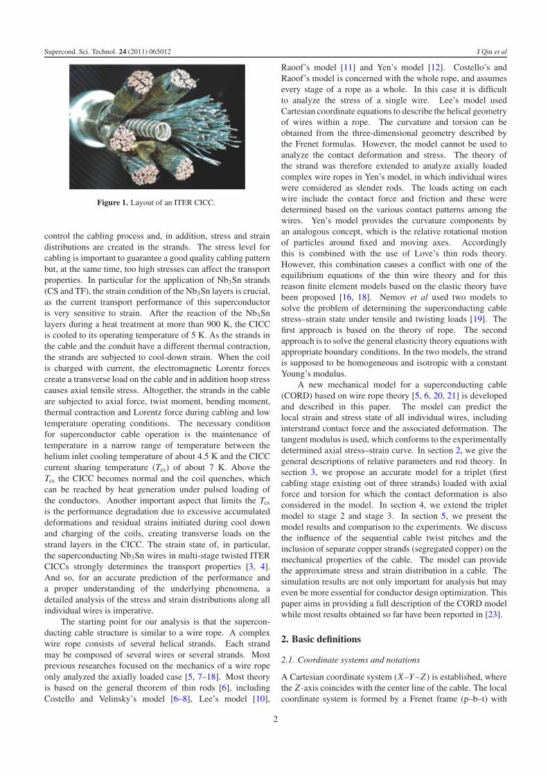
CICCs) in their turn have different layouts. The key point ina CICC is the superconductor cable. The cable of more than1000 strands is build up from different cabling stages with adiameter of 0.8 mm and a void fraction of 30% for optimalhelium cooling, see figure 1.

The cable is enclosed in a (stainless steel) conduitand a helium cooling channel in the axial center allowsa low pressure drop of the helium flow through the largeCICC sections in the coils. Already in the phase of cablemanufacturing, the strands are subjected to stress in order to

0953-2048/11/065012+11$33.00 © 2011 IOP Publishing Ltd Printed in the UK & the USA1

Supercond. Sci. Technol. 24 (2011) 065012 J Qin et al

Figure 1. Layout of an ITER CICC.

control the cabling process and, in addition, stress and straindistributions are created in the strands. The stress level forcabling is important to guarantee a good quality cabling patternbut, at the same time, too high stresses can affect the transportproperties. In particular for the application of Nb3Sn strands(CS and TF), the strain condition of the Nb3Sn layers is crucial,as the current transport performance of this superconductoris very sensitive to strain. After the reaction of the Nb3Snlayers during a heat treatment at more than 900 K, the CICCis cooled to its operating temperature of 5 K. As the strands inthe cable and the conduit have a different thermal contraction,the strands are subjected to cool-down strain. When the coilis charged with current, the electromagnetic Lorentz forcescreate a transverse load on the cable and in addition hoop stresscauses axial tensile stress. Altogether, the strands in the cableare subjected to axial force, twist moment, bending moment,thermal contraction and Lorentz force during cabling and lowtemperature operating conditions. The necessary conditionfor superconductor cable operation is the maintenance oftemperature in a narrow range of temperature between thehelium inlet cooling temperature of about 4.5 K and the CICCcurrent sharing temperature (Tcs) of about 7 K. Above theTcs the CICC becomes normal and the coil quenches, whichcan be reached by heat generation under pulsed loading ofthe conductors. Another important aspect that limits the Tcs

is the performance degradation due to excessive accumulateddeformations and residual strains initiated during cool downand charging of the coils, creating transverse loads on thestrand layers in the CICC. The strain state of, in particular,the superconducting Nb3Sn wires in multi-stage twisted ITERCICCs strongly determines the transport properties [3, 4].And so, for an accurate prediction of the performance anda proper understanding of the underlying phenomena, adetailed analysis of the stress and strain distributions along allindividual wires is imperative.

The starting point for our analysis is that the supercon-ducting cable structure is similar to a wire rope. A complexwire rope consists of several helical strands. Each strandmay be composed of several wires or several strands. Mostprevious researches focused on the mechanics of a wire ropeonly analyzed the axially loaded case [5, 7–18]. Most theoryis based on the general theorem of thin rods [6], includingCostello and Velinsky’s model [6–8], Lee’s model [10],

Raoof’s model [11] and Yen’s model [12]. Costello’s andRaoof’s model is concerned with the whole rope, and assumesevery stage of a rope as a whole. In this case it is difficultto analyze the stress of a single wire. Lee’s model usedCartesian coordinate equations to describe the helical geometryof wires within a rope. The curvature and torsion can beobtained from the three-dimensional geometry described bythe Frenet formulas. However, the model cannot be used toanalyze the contact deformation and stress. The theory ofthe strand was therefore extended to analyze axially loadedcomplex wire ropes in Yen’s model, in which individual wireswere considered as slender rods. The loads acting on eachwire include the contact force and friction and these weredetermined based on the various contact patterns among thewires. Yen’s model provides the curvature components byan analogous concept, which is the relative rotational motionof particles around fixed and moving axes. Accordinglythis is combined with the use of Love’s thin rods theory.However, this combination causes a conflict with one of theequilibrium equations of the thin wire theory and for thisreason finite element models based on the elastic theory havebeen proposed [16, 18]. Nemov et al used two models tosolve the problem of determining the superconducting cablestress–strain state under tensile and twisting loads [19]. Thefirst approach is based on the theory of rope. The secondapproach is to solve the general elasticity theory equations withappropriate boundary conditions. In the two models, the strandis supposed to be homogeneous and isotropic with a constantYoung’s modulus.

A new mechanical model for a superconducting cable(CORD) based on wire rope theory [5, 6, 20, 21] is developedand described in this paper. The model can predict thelocal strain and stress state of all individual wires, includinginterstrand contact force and the associated deformation. Thetangent modulus is used, which conforms to the experimentallydetermined axial stress–strain curve. In section 2, we give thegeneral descriptions of relative parameters and rod theory. Insection 3, we propose an accurate model for a triplet (firstcabling stage existing out of three strands) loaded with axialforce and torsion for which the contact deformation is alsoconsidered in the model. In section 4, we extend the tripletmodel to stage 2 and stage 3. In section 5, we present themodel results and comparison to the experiments. We discussthe influence of the sequential cable twist pitches and theinclusion of separate copper strands (segregated copper) on themechanical properties of the cable. The model can providethe approximate stress and strain distribution in a cable. Thesimulation results are not only important for analysis but mayeven be more essential for conductor design optimization. Thispaper aims in providing a full description of the CORD modelwhile most results obtained so far have been reported in [23].

2. Basic definitions

2.1. Coordinate systems and notations

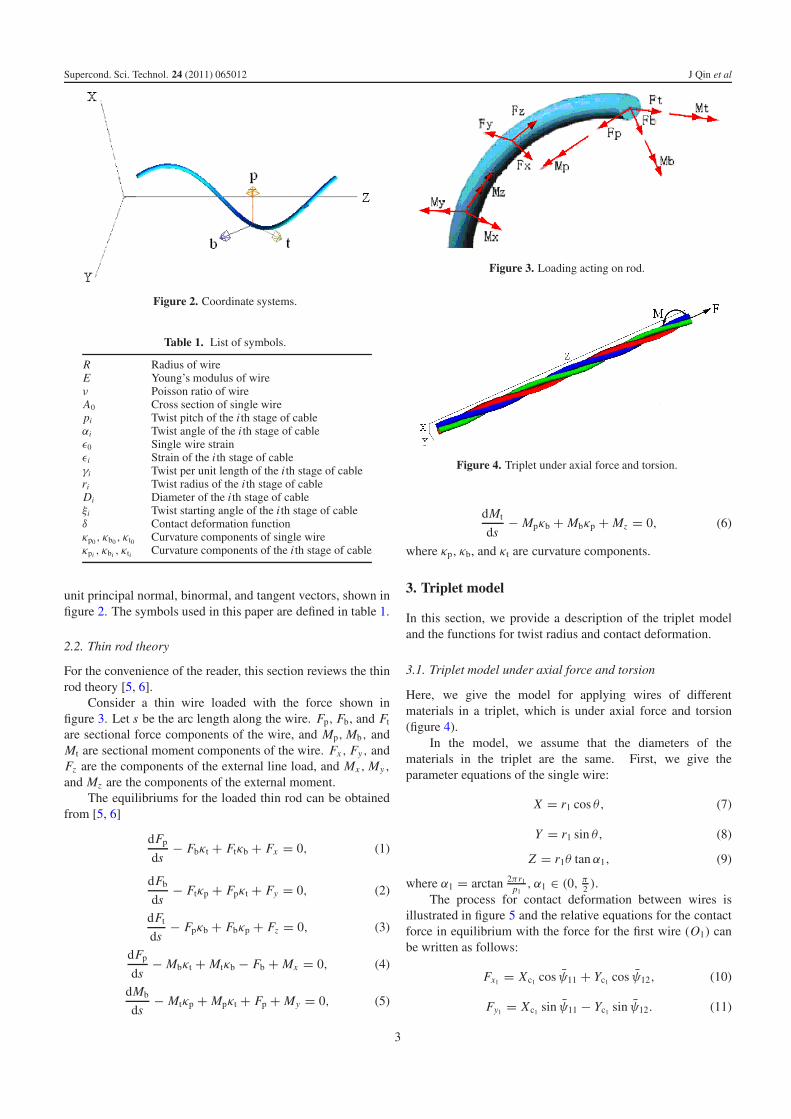
A Cartesian coordinate system (X–Y –Z ) is established, wherethe Z -axis coincides with the center line of the cable. The localcoordinate system is formed by a Frenet frame (p–b–t) with

2

Supercond. Sci. Technol. 24 (2011) 065012 J Qin et al

Figure 2. Coordinate systems.

Table 1. List of symbols.

R Radius of wireE Young’s modulus of wireν Poisson ratio of wireA0 Cross section of single wirepi Twist pitch of the i th stage of cableαi Twist angle of the i th stage of cableε0 Single wire strainεi Strain of the i th stage of cableγi Twist per unit length of the i th stage of cableri Twist radius of the i th stage of cableDi Diameter of the i th stage of cableξi Twist starting angle of the i th stage of cableδ Contact deformation functionκp0 , κb0 , κt0 Curvature components of single wireκpi , κbi , κti Curvature components of the i th stage of cable

unit principal normal, binormal, and tangent vectors, shown infigure 2. The symbols used in this paper are defined in table 1.

2.2. Thin rod theory

For the convenience of the reader, this section reviews the thinrod theory [5, 6].

Consider a thin wire loaded with the force shown infigure 3. Let s be the arc length along the wire. Fp, Fb, and Ft

are sectional force components of the wire, and Mp,Mb, andMt are sectional moment components of the wire. Fx , Fy, andFz are the components of the external line load, and Mx ,My ,

and Mz are the components of the external moment.The equilibriums for the loaded thin rod can be obtained

from [5, 6]

dFp

ds− Fbκt + Ftκb + Fx = 0, (1)

dFb

ds− Ftκp + Fpκt + Fy = 0, (2)

dFt

ds− Fpκb + Fbκp + Fz = 0, (3)

dFp

ds− Mbκt + Mtκb − Fb + Mx = 0, (4)

dMb

ds− Mtκp + Mpκt + Fp + My = 0, (5)

Figure 3. Loading acting on rod.

Figure 4. Triplet under axial force and torsion.

dMt

ds− Mpκb + Mbκp + Mz = 0, (6)

where κp, κb, and κt are curvature components.

3. Triplet model

In this section, we provide a description of the triplet modeland the functions for twist radius and contact deformation.

3.1. Triplet model under axial force and torsion

Here, we give the model for applying wires of differentmaterials in a triplet, which is under axial force and torsion(figure 4).

In the model, we assume that the diameters of thematerials in the triplet are the same. First, we give theparameter equations of the single wire:

X = r1 cos θ, (7)

Y = r1 sin θ, (8)

Z = r1θ tanα1, (9)

where α1 = arctan 2πr1p1, α1 ∈ (0, π2 ).

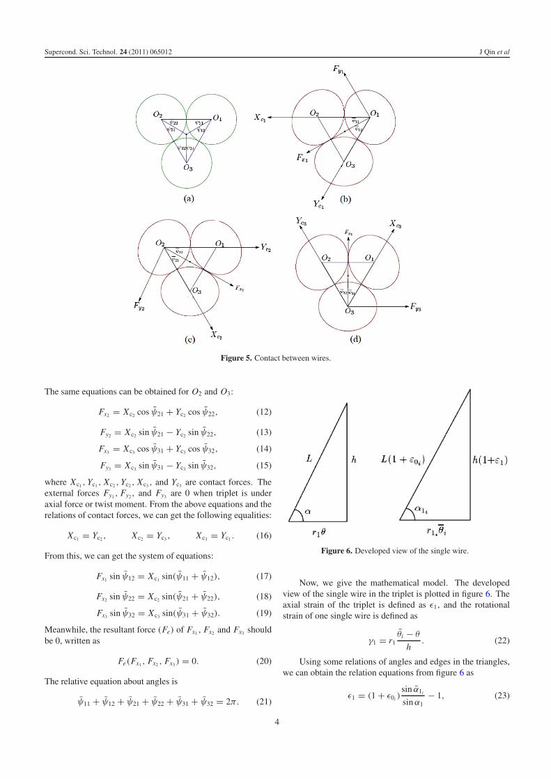
The process for contact deformation between wires isillustrated in figure 5 and the relative equations for the contactforce in equilibrium with the force for the first wire (O1) canbe written as follows:

Fx1 = Xc1 cos ψ11 + Yc1 cos ψ12, (10)

Fy1 = Xc1 sin ψ11 − Yc1 sin ψ12. (11)

3

Supercond. Sci. Technol. 24 (2011) 065012 J Qin et al

Figure 5. Contact between wires.

The same equations can be obtained for O2 and O3:

Fx2 = Xc2 cos ψ21 + Yc2 cos ψ22, (12)

Fy2 = Xc2 sin ψ21 − Yc2 sin ψ22, (13)

Fx3 = Xc3 cos ψ31 + Yc3 cos ψ32, (14)

Fy3 = Xc3 sin ψ31 − Yc3 sin ψ32, (15)

where Xc1 ,Yc1 , Xc2 ,Yc2 , Xc3 , and Yc3 are contact forces. Theexternal forces Fy1 , Fy2, and Fy3 are 0 when triplet is underaxial force or twist moment. From the above equations and therelations of contact forces, we can get the following equalities:

Xc1 = Yc2 , Xc2 = Yc3 , Xc3 = Yc1 . (16)

From this, we can get the system of equations:

Fx1 sin ψ12 = Xc1 sin(ψ11 + ψ12), (17)

Fx2 sin ψ22 = Xc2 sin(ψ21 + ψ22), (18)

Fx3 sin ψ32 = Xc3 sin(ψ31 + ψ32). (19)

Meanwhile, the resultant force (Fe) of Fx1 , Fx2 and Fx3 shouldbe 0, written as

Fe(Fx1 , Fx2 , Fx3 ) = 0. (20)

The relative equation about angles is

ψ11 + ψ12 + ψ21 + ψ22 + ψ31 + ψ32 = 2π. (21)

Figure 6. Developed view of the single wire.

Now, we give the mathematical model. The developedview of the single wire in the triplet is plotted in figure 6. Theaxial strain of the triplet is defined as ε1, and the rotationalstrain of one single wire is defined as

γ1 = r1θi − θ

h. (22)

Using some relations of angles and edges in the triangles,we can obtain the relation equations from figure 6 as

ε1 = (1 + ε0i )sin α1i

sinα1− 1, (23)

4

Supercond. Sci. Technol. 24 (2011) 065012 J Qin et al

Figure 7. Contact between wires (left: before contact deformation; right: after contact deformation).

γ1 = r1

r1i

1 + ε1

tan α1i

− 1

tanα1. (24)

The original components of the curvature and the twist perunit length are

κp0 = 0, κb0 = cos2 α1

r1, κt0 = sinα1 cosα1

r1.

The components of the curvature and the twist per unitlength of every wire under loading are

κp0i= 0, κb0i

= cos2 α1i

r1i

, κt0i= sin α1i cos α1

r1i

.

In the analysis, a wire is regarded as a thin rod, and thesectional moments are related to the changes of curvature andtorsion. The moments of a single wire can be obtained with

Mpi = Ei Ipi (κp0i− κp0), (25)

Mbi = Ei Ibi (κb0i− κb0), (26)

Mti = Ei Iti (κt0i− κt0). (27)

The axial force in the single wire is given by

Fti = A0σi (ε0i ). (28)

According to the above equilibrium of a thin wire, the sectionalshear forces and contact force can be expressed by

Fpi = −dMbi

ds+ Mti · κp0i

− Mpi · κt0i, (29)

Fbi = dMpi

ds− Mbi · κt0i

+ Mti · κb0i, (30)

Fxi = Fbi · κt0i− Fti · κb0i

. (31)

The total axial force F and the total axial twisting moment Macting on the triplet can be obtained by

F = 3i=1(Fti sinα1 + Fbi cosα1), (32)

M = 3i=1(Mti sinα1+Mbi cosα1+Fti r1 cosα1−Fbi r1 sinα1).

(33)There are nineteen unknown quantities in the model,

which are F,M, Xc1 , Xc2 , Xc3 , ψ11, ψ12, ψ21, ψ22, ψ31, ψ32,

ε1, ε01 , ε02 , ε03 , γ1, α11 , α12 , and α13 . The relative equationsare equations (17)–(24), equations (32) and (33) and sometriangle relationship equations. The system of equations isnonlinear. Therefore, we apply the Newton method to solveit when we know the values of two quantities. Generally, wesolve the system of equations with known axial force (F) andtwist moment (M) or ε1 and γ1.

3.2. Functions of changed twist radius and contactdeformation

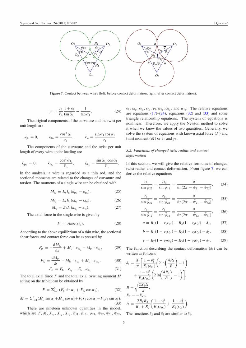
In this section, we will give the relative formulas of changedtwist radius and contact deformation. From figure 7, we canderive the relative equations

r11

sin ψ22= r12

sin ψ11= a

sin(2π − ψ11 − ψ22), (34)

r12

sin ψ32= r13

sin ψ21= a

sin(2π − ψ21 − ψ32), (35)

r13

sin ψ12= r11

sin ψ31= a

sin(2π − ψ12 − ψ31), (36)

a = R1(1 − ν1ε01)+ R2(1 − ν2ε02)− δ1, (37)

b = R1(1 − ν1ε01)+ R3(1 − ν3ε03)− δ2, (38)

c = R2(1 − ν2ε02)+ R3(1 − ν3ε03)− δ3. (39)

The function describing the contact deformation (δ1) can bewritten as follows:

δ1 = X f

π

[1 − ν2

1

E1(ε01)

(2 ln

(4R1

B

)− 1

)

+ 1 − ν22

E2(ε02)

(2 ln

(4R2

B

)− 1

)],

B =√

2X f�

π,

X f = −Xci ,

� = 2R1 R2

R1 + R2

(1 − ν2

1

E1(ε01)+ 1 − ν2

2

E2(ε02)

).

The functions δ2 and δ3 are similar to δ1.

5

Supercond. Sci. Technol. 24 (2011) 065012 J Qin et al

Figure 8. Second stage under axial force and torsion.

4. The model for the second stage and third stage

In this section, we present the models for stages 2 and 3 forwhich an analogous approach is followed.

4.1. The model for the second stage

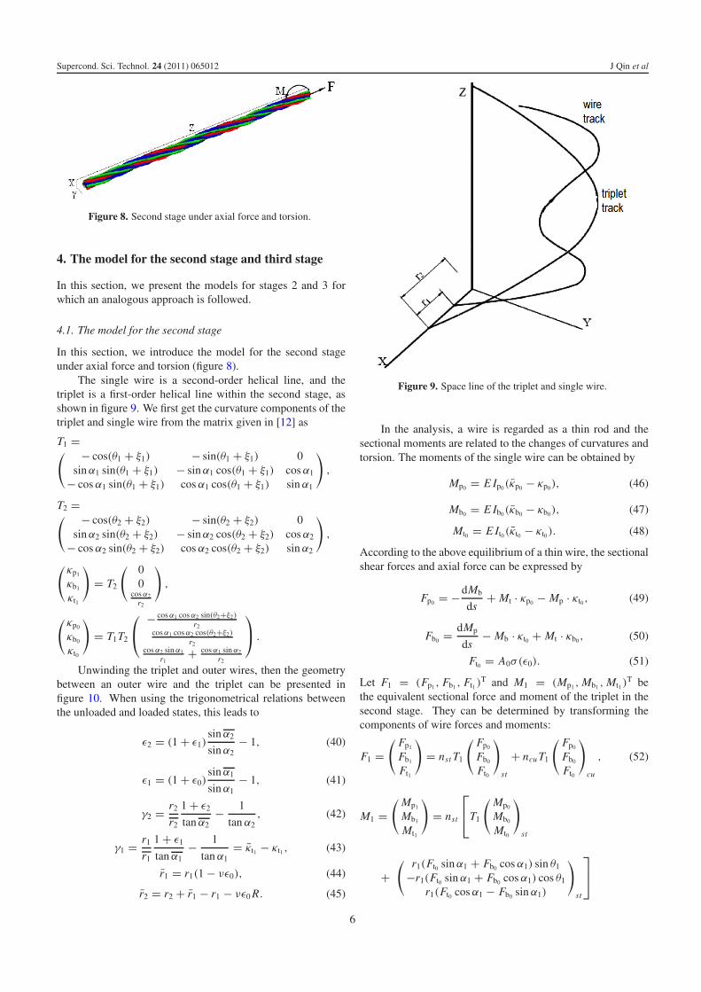
In this section, we introduce the model for the second stageunder axial force and torsion (figure 8).

The single wire is a second-order helical line, and thetriplet is a first-order helical line within the second stage, asshown in figure 9. We first get the curvature components of thetriplet and single wire from the matrix given in [12] as

T1 =( − cos(θ1 + ξ1) − sin(θ1 + ξ1) 0sinα1 sin(θ1 + ξ1) − sinα1 cos(θ1 + ξ1) cosα1

− cosα1 sin(θ1 + ξ1) cosα1 cos(θ1 + ξ1) sinα1

),

T2 =( − cos(θ2 + ξ2) − sin(θ2 + ξ2) 0sinα2 sin(θ2 + ξ2) − sinα2 cos(θ2 + ξ2) cosα2

− cosα2 sin(θ2 + ξ2) cosα2 cos(θ2 + ξ2) sinα2

),

(κp1

κb1

κt1

)= T2

( 00

cosα2r2

),

(κp0

κb0

κt0

)= T1T2

⎛⎝

− cosα1 cosα2 sin(θ2+ξ2)

r2cosα1 cosα2 cos(θ2+ξ2)

r2cosα2 sin α1

r1+ cosα1 sinα2

r2

⎞⎠ .

Unwinding the triplet and outer wires, then the geometrybetween an outer wire and the triplet can be presented infigure 10. When using the trigonometrical relations betweenthe unloaded and loaded states, this leads to

ε2 = (1 + ε1)sinα2

sinα2− 1, (40)

ε1 = (1 + ε0)sinα1

sinα1− 1, (41)

γ2 = r2

r2

1 + ε2

tanα2− 1

tanα2, (42)

γ1 = r1

r1

1 + ε1

tanα1− 1

tanα1= κt1 − κt1 , (43)

r1 = r1(1 − νε0), (44)

r2 = r2 + r1 − r1 − νε0 R. (45)

Figure 9. Space line of the triplet and single wire.

In the analysis, a wire is regarded as a thin rod and thesectional moments are related to the changes of curvatures andtorsion. The moments of the single wire can be obtained by

Mp0 = E Ip0(κp0 − κp0), (46)

Mb0 = E Ib0(κb0 − κb0), (47)

Mt0 = E It0(κt0 − κt0). (48)

According to the above equilibrium of a thin wire, the sectionalshear forces and axial force can be expressed by

Fp0 = −dMb

ds+ Mt · κp0 − Mp · κt0, (49)

Fb0 = dMp

ds− Mb · κt0 + Mt · κb0, (50)

Ft0 = A0σ(ε0). (51)

Let F1 = (Fp1, Fb1 , Ft1 )T and M1 = (Mp1 ,Mb1 ,Mt1 )

T bethe equivalent sectional force and moment of the triplet in thesecond stage. They can be determined by transforming thecomponents of wire forces and moments:

F1 =( Fp1

Fb1

Ft1

)= nst T1

( Fp0

Fb0

Ft0

)

st

+ ncu T1

( Fp0

Fb0

Ft0

)

cu

, (52)

M1 =(Mp1

Mb1

Mt1

)= nst

⎡⎣T1

(Mp0

Mb0

Mt0

)

st

+( r1(Ft0 sinα1 + Fb0 cosα1) sin θ1

−r1(Ft0 sinα1 + Fb0 cosα1) cos θ1

r1(Ft0 cosα1 − Fb0 sinα1)

)

st

⎤⎦

6

Supercond. Sci. Technol. 24 (2011) 065012 J Qin et al

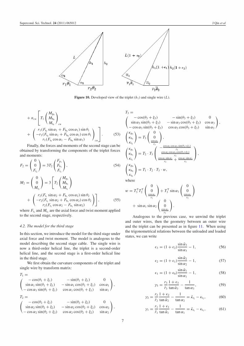
Figure 10. Developed view of the triplet (h1) and single wire (L).

+ ncu

⎡⎣T1

(Mp0

Mb0

Mt0

)

cu

+( r1(Ft0 sinα1 + Fb0 cosα1) sin θ1

−r1(Ft0 sinα1 + Fb0 cosα1) cos θ1

r1(Ft0 cosα1 − Fb0 sinα1)

)

cu

⎤⎦ . (53)

Finally, the forces and moments of the second stage can beobtained by transforming the components of the triplet forcesand moments:

F2 =( 0

0Ft2

)= 3T2

( Fp1

Fb1

Ft1

), (54)

M2 =( 0

0Mt2

)= 3

[T2

(Mp1

Mb1

Mt1

)

+( r2(Ft1 sinα2 + Fb1 cosα2) sin θ2

−r2(Ft1 sinα2 + Fb1 cosα2) cos θ2

r2(Ft1 cosα2 − Fb1 sinα2)

)], (55)

where Ft2 and Mt2 are the axial force and twist moment appliedto the second stage, respectively.

4.2. The model for the third stage

In this section, we introduce the model for the third stage underaxial force and twist moment. The model is analogous to themodel describing the second stage cable. The single wire isnow a third-order helical line, the triplet is a second-orderhelical line, and the second stage is a first-order helical linein the third stage.

We first obtain the curvature components of the triplet andsingle wire by transform matrix:

T1 =( − cos(θ1 + ξ1) − sin(θ1 + ξ1) 0sinα1 sin(θ1 + ξ1) − sinα1 cos(θ1 + ξ1) cosα1

− cosα1 sin(θ1 + ξ1) cosα1 cos(θ1 + ξ1) sinα1

),

T2 =( − cos(θ2 + ξ2) − sin(θ2 + ξ2) 0sinα2 sin(θ2 + ξ2) − sinα2 cos(θ2 + ξ2) cosα2

− cosα2 sin(θ2 + ξ2) cosα2 cos(θ2 + ξ2) sinα2

),

T3 =( − cos(θ3 + ξ3) − sin(θ3 + ξ3) 0sinα3 sin(θ3 + ξ3) − sinα3 cos(θ3 + ξ3) cosα3

− cosα3 sin(θ3 + ξ3) cosα3 cos(θ3 + ξ3) sinα3

),

(κp2

κb2

κt2

)= T3

( 00

cosα3r3

),

(κp1

κb1

κt1

)= T2 · T3

⎛⎝

− cosα2 cosα3 sin(θ3+ξ3)

r3cosα2 cosα3 cos(θ3+ξ3)

r3cosα3 sin α2

r2+ cosα2 sin α3

r3

⎞⎠ ,

(κp0

κb0

κt0

)= T1 · T2 · T3 ·w,

where

w = T T3 T T

2

( 00

cosα1r1

)+ T T

3 sinα1

( 00

cosα2r2

)

+ sinα1 sinα2

( 00

cosα3r3

).

Analogous to the previous case, we unwind the tripletand outer wires, then the geometry between an outer wireand the triplet can be presented as in figure 11. When usingthe trigonometrical relations between the unloaded and loadedstates, we can write

ε3 = (1 + ε2)sin α3

sinα3− 1, (56)

ε2 = (1 + ε1)sin α2

sinα2− 1, (57)

ε1 = (1 + ε0)sin α1

sinα1− 1, (58)

γ3 = r3

r3

1 + ε3

tan α3− 1

tanα3, (59)

γ2 = r2

r2

1 + ε2

tan α2− 1

tanα2= κt2 − κt2 , (60)

γ1 = r1

r1

1 + ε1

tan α1− 1

tanα1= κt1 − κt1 , (61)

7

Supercond. Sci. Technol. 24 (2011) 065012 J Qin et al

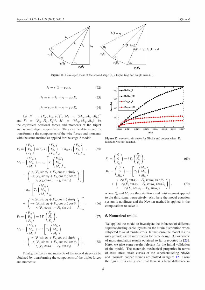
Figure 11. Developed view of the second stage (h2), triplet (h1) and single wire (L).

r1 = r1(1 − νε0), (62)

r2 = r2 + r1 − r1 − νε0 R, (63)

r3 = r3 + r2 − r2 − νε0 R. (64)

Let F1 = (Fp1 , Fb1 , Ft1)T, M1 = (Mp1 ,Mb1 ,Mt1 )

T

and F2 = (Fp2 , Fb2 , Ft2)T, M2 = (Mp2 ,Mb2 ,Mt2 )

T bethe equivalent sectional forces and moments of the tripletand second stage, respectively. They can be determined bytransforming the components of the wire forces and momentswith the same method as applied for the stage 2 model:

F1 =( Fp1

Fb1

Ft1

)= nst T1

( Fp0

Fb0

Ft0

)

st

+ ncu T1

( Fp0

Fb0

Ft0

)

cu

, (65)

M1 =(Mp1

Mb1

Mt1

)= nst

⎡⎣T1

(Mp0

Mb0

Mt0

)

st

+( r1(Ft0 sinα1 + Fb0 cosα1) sin θ1

−r1(Ft0 sinα1 + Fb0 cosα1) cos θ1

r1(Ft0 cosα1 − Fb0 sinα1)

)

st

⎤⎦

+ ncu

⎡⎣T1

(Mp0

Mb0

Mt0

)

cu

+( r1(Ft0 sinα1 + Fb0 cosα1) sin θ1

−r1(Ft0 sinα1 + Fb0 cosα1) cos θ1

r1(Ft0 cosα1 − Fb0 sinα1)

)

cu

⎤⎦ , (66)

F2 =( Fp2

Fb2

Ft2

)= 3T1

( Fp1

Fb1

Ft1

), (67)

M1 =(Mp1

Mb1

Mt1

)= 3

[T2

(Mp1

Mb1

Mt1

)

+( r2(Ft1 sinα2 + Fb1 cosα2) sin θ2

−r2(Ft1 sinα2 + Fb1 cosα2) cos θ2

r2(Ft1 cosα1 − Fb1 sinα2)

)]. (68)

Finally, the forces and moments of the second stage can beobtained by transforming the components of the triplet forcesand moments:

Figure 12. stress–strain curve for Nb3Sn and copper wires, R:reacted; NR: not reacted.

F3 =( 0

0Ft2

)= 5T3

( Fp2

Fb2

Ft2

), (69)

M3 =( 0

0Mt3

)= 3

[T3

(Mp2

Mb2

Mt2

)

+( r3(Ft2 sinα3 + Fb2 cosα3) sin θ3

−r3(Ft2 sinα3 + Fb2 cosα3) cos θ3

r3(Ft2 cosα3 − Fb2 sinα3)

)], (70)

where Ft3 and Mt3 are the axial force and twist moment appliedto the third stage, respectively. Also here the model equationsystem is nonlinear and the Newton method is applied in thecomputations to solve it.

5. Numerical results

We applied the model to investigate the influence of differentsuperconducting cable layouts on the strain distribution whensubjected to axial tensile stress. In that sense the model resultsmay provide useful information for cable design. An overviewof most simulation results obtained so far is reported in [23].Here, we give some results relevant for the initial validationof the model. The materials mechanical properties in termsof axial stress–strain curves of the superconducting Nb3Snand ‘normal’ copper strands are plotted in figure 12. Fromthe figure, it is easily seen that there is a large difference in

8

Supercond. Sci. Technol. 24 (2011) 065012 J Qin et al

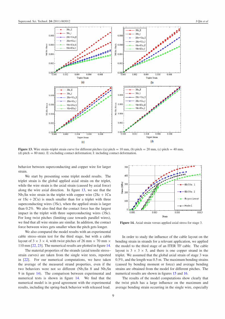
Figure 13. Wire strain–triplet strain curve for different pitches ((a) pitch = 10 mm, (b) pitch = 20 mm, (c) pitch = 40 mm,(d) pitch = 80 mm). E: excluding contact deformation; I: including contact deformation.

behavior between superconducting and copper wire for largerstrain.

We start by presenting some triplet model results. Thetriplet strain is the global applied axial strain on the triplet,while the wire strain is the axial strain (caused by axial force)along the wire axial direction. In figure 13, we see that theNb3Sn wire strain in the triplet with copper wire (2Sc + 1Cuor 1Sc + 2Cu) is much smaller than for a triplet with threesuperconducting wires (3Sc), when the applied strain is largerthan 0.2%. We also find that the contact force has the largestimpact in the triplet with three superconducting wires (3Sc).For long twist pitches (limiting case towards parallel wires),we find that all wire strains are similar. In addition, the contactforce between wires gets smaller when the pitch gets longer.

We also compared the model results with an experimentalcable stress–strain test for the third stage, but with a cablelayout of 3 × 3 × 4, with twist pitches of 26 mm × 70 mm ×110 mm [22, 23]. The numerical results are plotted in figure 14.

The material properties of the strands (axial tensile stress–strain curves) are taken from the single wire tests, reportedin [22]. For our numerical computations, we have takenthe average of the measured strand properties, even if thetwo behaviors were not so different (Nb3Sn 8 and Nb3Sn9 in figure 14). The comparison between experimental andnumerical tests is shown in figure 14. We find that thenumerical model is in good agreement with the experimentalresults, including the spring-back behavior with released load.

Figure 14. Axial strain versus applied axial stress for stage 3.

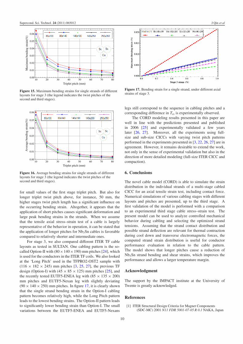
In order to study the influence of the cable layout on thebending strain in strands for a relevant application, we appliedthe model to the third stage of an ITER TF cable. The cablelayout is 3 × 3 × 5, and there is one copper strand in thetriplet. We assumed that the global axial strain of stage 3 was0.5%, and the length was 0.5 m. The maximum bending strains(caused by bending moment or force) and average bendingstrains are obtained from the model for different pitches. Thenumerical results are shown in figures 15 and 16.

The results of the model computations show clearly thatthe twist pitch has a large influence on the maximum andaverage bending strain occurring in the single wire, especially

9

Supercond. Sci. Technol. 24 (2011) 065012 J Qin et al

Figure 15. Maximum bending strains for single strands of differentlayouts for stage 3 (the legend indicates the twist pitches of thesecond and third stages).

Figure 16. Average bending strains for single strands of differentlayouts for stage 3 (the legend indicates the twist pitches of thesecond and third stages).

for small values of the first stage triplet pitch. But also forlonger triplet twist pitch above, for instance, 50 mm, thehigher stages twist pitch length has a significant influence onthe occurring bending strain. Altogether, it appears that theapplication of short pitches causes significant deformation andlarge peak bending strains in the strands. When we assumethat the tensile axial stress–strain test of a cable is largelyrepresentative of the behavior in operation, it can be stated thatthe application of longer pitches for Nb3Sn cables is favorablecompared to relatively shorter and intermediate ones.

For stage 3, we also compared different ITER TF cablelayouts as tested in SULTAN. One cabling pattern is the so-called Option-II with (80×140×190) mm pitches [24], whichis used for the conductors in the ITER TF coils. We also lookedat the ‘Long Pitch’ used in the TFPRO2-OST2 sample with(116 × 182 × 245) mm pitches [3, 25, 27], the previous TFdesign (Option-I) with (45 × 85 × 125) mm pitches [25], andthe recently tested EUTF5-ENEA leg with (85 × 135 × 200)mm pitches and EUTF5-Nexan leg with slightly deviating(90 × 140 × 250) mm pitches. In figure 17, it is clearly shownthat the single strand bending strain in the Option-I cablingpattern becomes relatively high, while the Long Pitch patternleads to the lowest bending strains. The Option-II pattern leadsto significantly lower bending strain than Option-I. The smallvariations between the EUTF5-ENEA and EUTF5-Nexans

Figure 17. Bending strain for a single strand, under different axialstrains of stage 3.

legs still correspond to the sequence in cabling pitches and acorresponding difference in Tcs is experimentally observed.

The CORD modeling results presented in this paper arewell in line with the predictions presented and publishedin 2006 [25] and experimentally validated a few yearslater [26, 27]. Moreover, all the experiments using full-size and sub-size CICCs with varying twist pitch patternsperformed in the experiments presented in [3, 22, 26, 27] are inagreement. However, it remains desirable to extend the work,not only in the sense of experimental validation but also in thedirection of more detailed modeling (full-size ITER CICC andcompaction).

6. Conclusions

The novel cable model (CORD) is able to simulate the straindistribution in the individual strands of a multi-stage cabledCICC for an axial tensile strain test, including contact force.Numerical simulations of various cabling stages with differentlayouts and pitches are presented, up to the third stage. Afirst validation of the model is performed with a comparisonto an experimental third stage cable stress–strain test. Thepresent model can be used to analyze controlled mechanicalbehavior during cabling and selecting the optimized strandtensions. Assuming that the strand contact distribution andpossible strand deflection are relevant for thermal contractionduring cool down and transverse electromagnetic forces, thecomputed strand strain distribution is useful for conductorperformance evaluation in relation to the cable pattern.The model shows that longer pitches cause a reduction ofNb3Sn strand bending and shear strains, which improves theperformance and allows a larger temperature margin.

Acknowledgment

The support by the IMPACT institute at the University ofTwente is greatly acknowledged.

References

[1] ITER Structural Design Criteria for Magnet Components(SDC-MC) 2001 N11 FDR 5001-07-05 R 0.1 NAKA, Japan

10

Supercond. Sci. Technol. 24 (2011) 065012 J Qin et al

[2] 2004 ITER Final Design Report IAEA Vienna and ITER ITteam Design Description Document 1.1 Update January

[3] Nijhuis A 2008 A solution for transverse load degradation inITER Nb3Sn CICCs: verification of cabling effect onLorentz force response Supercond. Sci. Technol. 21 054011

[4] van den Eijnden N C and Nijhuis A 2005 Axial tensilestress–strain characterization of ITER model coil typeNb3Sn strands in TARSIS Supercond. Sci. Technol. 18 1–10

[5] Costello G A 1997 Theory of Wire Rope 2nd edn (Berlin:Springer)

[6] Love A E H 1944 A Treatise on the Mathematical Theory ofElasticity (New York: Dover)

[7] Phillips J W and Costello G A 1979 Gernal axial response ofstranded wire helical springs Int. J. Non-Linear Mech.14 247–57

[8] Costello G A and Phillips J W 1979 Static response of strandedwire helical springs Int. J. Non-Linear Mech. 21 171–81

[9] Velinsky S A 1985 General nonlinear theory for complex wirerope Int. J. Mech. Sci. 27 497–507

[10] Lee W K 1991 An insight into wire rope geometry Int. J. SolidsStruct. 28 471–90

[11] Raoof M and Hobbs R E 1988 Analysis of multilayeredstructurestrands J. Eng. Mech., ASCE 114 1166–82

[12] Yen J and Chen C 2006 Theoretical approach to the solutions ofaxially loaded complex ropes J. Chin. Inst. Eng. 29 695–701

[13] Feyrer K 2007 Wire Ropes: Tension, Endurance, Reliability(Berlin: Springer)

[14] Kruijer M 2006 Modelling the time-dependent mechanicalbehaviour of steel reinforced thermo-plasticpipes PhDThesis

[15] Elata D, Eshkenazy R and Weiss M P 2004 The mechanicalbehaviour of a wire rope with an indepen-dent wire ropecore Int. J. Solids Struct. 41 1157–72

[16] Nawrocki A and Labrosse M 2000 A fnite element model forsimple straight wire rope strands Comput. Struct. 77 345–59

[17] Kusy R P and Dilley G J 1984 Elastic modulus of atriple-strand stainless steel arch wire via three-and four-pointbending J. Dent. Res. 63 1232–40

[18] Inagaki K, Ekh J and Zahrai S 2007 Mechanical analsis ofsecond order helical structure in electrical cable Int. J. SolidsStruct. 44 1657–79

[19] Nemov A S et al Generalized stiffness coefcients for ITERsuperconducting cables, direct FE modeling and initialconfguration Cryogenics 50 304–13

[20] Johnson K L 1985 Contact Mechanics (Cambridge: CambridgeUniversity Press)

[21] Gere J M and Timoshenko S P 1999 Mechanics of Materials(Cheltenham: Stanley Thornes Ltd)

[22] Ilyin Y, Nijhuis A, Wessel W A J, van den Eijnden N andten Kate H H J 2006 Axial tensile stress-straincharacterization of 36 Nb3Sn strands cable IEEE Trans.Appl. Supercond. 16 1249–52

[23] Qin J, Warnet L L, Wu Y and Nijhuis A 2008 CORD, a novelnumerical mechanical model for Nb3Sn CICCs IEEE Trans.Appl. Supercond. 18 1105–8

[24] Besi Vetrella U et al 2008 Manufacturing of the the ITER TFfull size prototype conductor IEEE Trans. Appl. Supercond.18 1105–8

[25] Nijhuis A and Ilyin Y 2006 Transverse load optimization inNb3Sn CICC design; influence of cabling, void fraction andstrand stiffness Supercond. Sci. Technol. 19 945–62

[26] Bruzzone P et al 2009 Test results of a Nb3Sn cable-in-conduitconductor with variable pitch sequence IEEE Trans. Appl.Supercond. 19 1448–51

[27] Bessette D and Mitchell N 2008 Review of the results of theITER toroidal field conductor R&D and qualification IEEETrans. Appl. Supercond. 18 1109–13

11