Embed Size (px)
Citation preview
applied sciences
Article
A Novel Approach to Model a Gas Network
Ali Ekhtiari 1 , Ioannis Dassios 2,*, Muyang Liu 2 and Eoin Syron 1
1 School of Chemical and Bioprocess Engineering, University College Dublin, Dublin 4, Ireland;[email protected] (A.E.); [email protected] (E.S.)
2 AMPSAS, University College Dublin, Dublin 4, Ireland; [email protected]* Correspondence: [email protected]
Received: 29 December 2018; Accepted: 6 March 2019; Published: 13 March 2019
Abstract: The continuous uninterrupted supply of Natural Gas (NG) is crucial to today’s economy,with issues in key infrastructure, e.g., Baumgarten hub in Austria in 2017, highlighting the importanceof the NG infrastructure for the supply of primary energy. The balancing of gas supply from a widerange of sources with various end users can be challenging due to the unique and different behavioursof the end users, which in some cases span across a continent. Further complicating the managementof the NG network is its role in supporting the electrical network. The fast response times of NGpower plants and the potential to store energy in the network play a key role in adding flexibilityacross other energy systems. Traditionally, modelling the NG network relies on nonlinear pipe flowequations that incorporate the demand (load), flow rate, and physical network parameters includingtopography and NG properties. It is crucial that the simulations produce accurate results quickly.This paper seeks to provide a novel method to solve gas flow equations through a network understeady-state conditions. Firstly, the model is reformulated into non-linear matrix equations, then theequations separated into their linear and nonlinear components, and thirdly, the non-linear systemis solved approximately by providing a linear system with similar solutions to the non-linear one.The non-linear equations of the NG transport system include the main variables and characteristicsof a gas network, focusing on pressure drop in the gas network. Two simplified models, both of theIrish gas network (1. A gas network with 13 nodes, 2. A gas network with 109 nodes) are used as acase study for comparison of the solutions. Results are generated by using the novel method, andthey are compared to the outputs of two numerical methods, the Newton–Raphson solution usingMATLAB and SAINT, a commercial software that is used for the simulation of the gas network andelectrical grids.
Keywords: non-linear system; discrete calculus; gas network model; gas flow equation
1. Introduction
The continuous uninterrupted supply of Natural Gas (NG) is crucial to today’s economy.The balancing of gas supply from a wide range of sources with various end users can be challengingdue to the unique and different behaviours of the end users, which in some cases span acrossa continent [1,2]. NG is one of the strategic primary sources of energy in the world, supplyingapproximately 24% of the world’s primary energy in 2016 [3]. This increases to 30% in Ireland, whereon occasion, 80% of peak power demand is provided by NG [4], and in Singapore, where generatedelectricity can be up to 95% [5] from NG. Transport of NG via pipeline is the most efficient andeconomic and has the lowest carbon footprint [6–8], and in many instances, the gas network is capableof supplying NG from gas fields directly to the end users (from Well to Wheels; WtW is a commonexpression for the life cycle of a product). A gas network includes both transmission and distributionpipelines, compressor stations to bring the transmission network to its operating pressure and City
Appl. Sci. 2019, 9, 1047; doi:10.3390/app9061047 www.mdpi.com/journal/applsci

Appl. Sci. 2019, 9, 1047 2 of 26
Gas reduction Stations (CGS) and Town Break Stations (TBS) to reduce the NG pressure so that itcan be provided safely into homes and business [9]. Gas systems need a reliable design to ensureeffective operation, and due to the important role of natural gas of supplying primary energy and thesignificant investment in the network infrastructure, using a reliable and fast method for solving thegas flow calculations is essential. Gas network simulation allows for the understanding and forecastof the behaviour of the gas network under different conditions, and it is useful for decision makersfor installing an optimal system. For the simulation of a gas network, the pipe flow equations thatdescribe the flow, pressure, compressibility, line-pack capacity, and density of the compressible gas inthe pipelines need to be solved. These equations include variables dependant on the gas composition,temperature, pipe length and diameter, gas constant, and pipe inclination, along with unknownvariables such as pressure and flow rate. The pressure and flow rate are the most important variablesfrom all points of view including financial/trading, technical, environmental, and health and safety.Gas network simulation helps the Transmission System Operator (TSO) understand how the individualcomponents work together as a system. It is crucial in planning for the development and expansion ofthe network, the prevention of faults due to system changes in supply or demand nodes [2], and inmanaging crisis events that occur due to catastrophic component failures. Furthermore, deviationsbetween accurate simulations and measured parameters can be an indication of leakage, which isimportant not just due to lost revenue point of view, but also from an environmental [10,11] andworker safety point of view. Therefore, accuracy is hugely important for simulations, where it can bethe difference between making a profit or loss for both the TSO and the retailer [12]. Validation of thesimulations requires reliable data, and robust reliable metering devices are key to ensuring this; theyare also crucial in custody transfer, which is becoming more important as gas markets are opening up.
Multiple variables affect gas flow through a pipeline, all of which must be accounted for in themodelling of the gas network; these are pressure, flow rate, density, comparability, friction factors,inclination of the pipe, the Reynolds number, gas velocity, and pipe length and diameter. The mostimportant variable in a gas network is pressure, which is the driving force for the transport of the NGthrough the pipe. When gas flows, the pressure decreases due to the frictional interaction between thegas and the pipe wall, exerting a shear force on the gas [2,13–17].
The modelling of the network topology also needs to be accounted for as it affects the gas pressureand has a major impact on the energy required to pump gas through the network. Each network hasits unique particular distribution/transmission characteristics, and changes at a node (supplier ordemand) will have consequences throughout the NG transport system [18]. In most countries, gas isdistributed by pipeline networks over a vast range of pressures [19]; these are mainly divided intotwo, high pressure and low pressure systems, which are specified for transmission and distributionlines, respectively. However, in some research simulations, e.g., [18], middle-pressure pipelines arealso investigated. Very large users of NG, such as power stations, are supplied directly from thetransmission network, while other users including residential users receive NG via the distributionnetwork [20]. A gas network is generally represented by a diagram involving branches (pipelines)and nodes (pipe connections). Facilities and equipment can be divided two groups: active and/orpassive [21]. An active node or branch represents a actively-controlled facility, which is controlledduring operation, e.g., compressors, regulator valves, and town gate stations. On the other side,the passive equipment will exert an influence on the network; however, its impact is due to the flowconditions, and the device is not adjusted or controlled. The prime example of passive equipment isthe pipes [13].
Gas networks are large infrastructures with significant interconnection to the other networks,mainly electrical grids. Therefore, the security of gas supply is important to ensure continuingelectricity supply. The challenge in gas networks is to balance the supply from different sources, withthe changing demand. By controlling the pressure of the network, the TSO can ensure that sufficientgas is available to supply the end users with sufficient quantities. In this paper, a novel method isused to solve the non-linear system of algebraic equations. It provides a matrix formulation of the

Appl. Sci. 2019, 9, 1047 3 of 26
non-linear system describing the model, and by using matrix algebra, an alternative linear systemis created. The solution of the alternative linear system can be used as a smooth approximation ofthe solutions of the non-linear system. This formulation is ready for software implementation andmay also be used in atomic scale models as an alternative to existing empirical approaches with pairand cohesive potentials. An illustrative example, analysing a local region of a node, is presented todemonstrate the model performance.
In this study, two simplified gas networks were created, each based on the Irish Gas Network.Network 1 is A gas network with 13 nodes and 14 pipes, and a bigger network, Network 2, has109 nodes and 112 pipes. Both networks are used for comparison of the novel approach with numericalsolutions. Having a new reliable method for gas network modelling with fast calculation and preciseresults can be an option to replace numerical solutions, especially for large gas networks, such as thosein continental Europe or North America, which contain several hundred nodes and pipelines andwhere large computation power is required. This new approach is a computational method that helpsin producing faster results, and when the modelling of NG networks is coupled with other energysystems, for example the electrical network, faster and less computationally-demanding results are ofkey importance.
2. Literature Review
Various methods have been published to model a gas network and solve the governing equationsof gas flow through the pipelines, with the vast majority applying numerical methods due to thenon-linearity of the equations. In the literature, a Steady-State Model (SSM) is frequently used wherethe pressure (the driving force) and flow rate at the inlet and outlet of the pipeline are assumedconstant. The steady-state equations of gas flow are non-linear algebraic, and in most cases, forsolving this type of equation, numerical solutions are employed. Some valuable studies of SSM havebeen published. The principles and fundamentals of graph theory can be used to model a networkalong with the empirical flow equations for low-, medium-, and high-pressure flow. Various differentempirical flow equations have been proposed such as Lacey’s equation, the Polyflo equation, thePanhandle equation, and the Weymouth equation (for high-pressure networks). Osiadacz [19] appliedthe Newton–Raphson method to deal with the non-linear equations. In this work, a step-by-step,Newton–Raphson method using a Jacobian matrix in graph theory was presented to model a horizontalgas pipe network. The essence of the work is the presentation of a computational method based onphysical and mathematical laws for simplification of fundamental equations. While this work is oneof the leading references in the modelling of gas networks, no specified example for a pipeline withinclination was presented. Many authors for simplification neglect the inclination term; however,Matko, Kwabena, and Iterran-Gonzales [22–25] are some authors who have considered inclinationin the pipe flow equation, because of its importance for the validation of models with real-worlddata. Simulation of a natural gas network focusing on gas quality using a numerical-iteration methodwas carried out by Abeysekera [26]. An important point of this literature is the inclusion of gaseswith different density in the network. Varying gas composition will impact gas pipeline systemcharacteristics such as pressure and flow rate. With a move to decarbonise the NG network, this isvital in the evaluation of the networks’ ability to store synthetic natural gas or hydrogen. Szoplik [18],after describing three different gas networks, low, middle, and high pressure, indicated two methodsto run the gas system model, which are the nodal method and loop method. In the nodal method, theflow rate is the dependent variable, and the pressure drop (differential pressures between two nodes ofa pipe/branch) through each branch is the independent variable Qij = f (dPij), while the loop methoddescribes that pressure is a function of flow rate (Equation (1)). The article investigates the impact ofambient temperature on the flow rate.
dPij = f (Qij) (1)

Appl. Sci. 2019, 9, 1047 4 of 26
Debebe’s [27] paper focused on simulation of transmission pipelines in a gas network focusingon compressor stations. The equations are mainly based on the mass balance, flow principles,and compression characteristics of gas in pipes. The Newton–Raphson method has been applied tosolve the equation using C++. The model evaluated the energy consumption for various configurationsin order to optimize the transmission pipeline flow and pressure. There are a number of papers thathave implemented the MATLAB-Simulink tool to simulate pipelines: Behbahani and Bagheri [28]and Herran-Gonzalez in [24] applied the Simulink toolbox in MATLAB to model the gas network.Behbahani and Bagheri [28] have manipulated the Simulink model of a gas system, and in order toverify the accuracy, the results have been compared with outputs from the finite difference scheme(FSM) and experimental test cases. The proposed model can predict the transient response of thedependent variable (pressure) with a good correlation with the nonlinear finite difference models.Herran [24] has implemented two models, the characteristic method and Crank–Nicholson, bothusing the MATLAB-Simulink library for solving the partial differential equations. The results for asimple triangle gas network (including two demand nodes and one supplier node) for both modelsproduced similar results to the Osiadacz model [19]. Mohring [29] applied a numerical method to runthe simplified loop model of a gas network. In this study, the inclination term has been neglected, andduring simplification, the compressibility term was held constant. Matko [25] discussed the non-linearequations and presented a solution by linearizing the unsteady-state equations where density, viscosity,and temperature (in adiabatic flow) are constant, but in reality, the non-linear flow equation consists ofa number of interdependent variables, e.g., flow through a pipeline gas flow rate relates the squares ofthe inlet and outlet pressures [30].
Yue-Wu [31] believed there were two important aspects in the modelling of gas systems; numericalsolutions and optimization, where a numerical solution is applied to determine the actual behaviour ofgas flow in the pipe. However, it is highlighted that the disadvantage of the numerical method is thatit is not able to put constraints on the system to find minimal cost, which is necessary for optimization.Furthermore, due to the fact that sizing of pipe diameters depends on the users’ demand, optimizationcould lead to significant operational advantages. The aim of optimization is to find the best set ofcontrol variables within a single optimization run. For some recent optimization methods useful forthis we refer to [32–34].
Along with the equation parameters, the solving of non-linear equations is dependent on both theinitial conditions and tolerance level chosen by the programmers, which can increase the computationaltime required and impact the convergence of the model (accuracy of the solution). Alternative methodsof solving the pipe flow equations such as the one presented in this work are therefore of interest,as when a large-scale network is modelled, the numerical iteration method will take more time to solvethe equations.
In recent years, there has been a significant development in using matrix theory to study networksrelated to engineering problems [35–38] and the solutions of non-linear algebraic systems [39–45].The idea is to provide new techniques and methods ready for software implementation in order tosolve non-linear equations, similar to those for modelling gas pipelines.
This paper presents a novel method for solving the equations governing flow and pressure in anatural gas network using matrix theory to derive a unique theorem.
3. Modelling of a Gas Network
A large amount of NG is transported long distances through the high-pressure pipeline network.Therefore, modelling/simulating of a gas transmission system with sufficient accuracy and fastcalculations methods is beneficial in understanding how the system will behave. Evaluation of thefeasibility of networks to cope with new customers, as well as the ability to determine the capacityof the current network, or to forecast the response of the system to any changes in supplying nodes(decrease/outage), as well as designing new gas network systems are areas where modelling can beused. The differential equations are used depending on the working pressure of the network and the

Appl. Sci. 2019, 9, 1047 5 of 26
operational conditions [19]. The major equations that must be satisfied in modelling gas flow in apipeline are:
• Mass conservation equation (equation of continuity).• Newton’s second law of motion (conservation of momentum).• Energy equation (thermodynamic first law) and the equation of state.
According to forces’ directions in a pipe, the governing equation has been extracted, which isshown in Figure 1 and from Newton’s second law of motion-momentum Equation (3).
Figure 1. Forces effective on a specific volume of gas flow through a pipeline.
The common equation for the steady-state flow of gas through a pipe is derived from Bernoulli’sequation of fluid flow, including changing density of gas due to the pressure drop along the pipe in thedirection of flow. The equation of mass conservation from inlet Point (1) to outlet Point (2) is shown inEquation (2).
ρ1w1 = ρ2w2 (2)
where ρ is density and ω represents flow velocity.
∂ρ
∂t+
∂(ρw)
∂x= 0 (3)
Newton’s second law of motion (conservation of momentum) in Equation (4):
∂(ρw)
∂t+
∂(ρw2)
∂x+
∂p∂x
+f ρw|w|
2D+ ρgsin(θ) = 0 (4)
where the following terms describe each portion of Equation (4):
∂(ρw)
∂t: inertia force (acting against the flow direction through the pipe)
∂(ρw2)
∂x: convective term

Appl. Sci. 2019, 9, 1047 6 of 26
∂p∂x
: pressure force
f ρw|w|2D
: shear force
ρgsin(θ): force of gravity
The variable pressure, p, and displacement, x, have been changed to p + dp and x + dx,respectively, which have been identified in Bernoulli’s Equation (5):
pρg
+w2
2g+ z =
p + dpρg
+(w + dw)2
2g+ (z + dz) + dh f (5)
where “dh f ” is the head losses, i and j are sending and receiving nodes, respectively, and “z” is pipeelevation. The first law of thermodynamics expresses the conservation of energy and for a system maybe written as:
Ω−W = ∆E (6)
where “Ω” is the heat added to the system, “W” is the work done by the system, and “E” is the changein energy of the system. Energy associated with the mass of the system is customarily separated intothree parts:
E = U +12
mw2 + mgz (7)
where “U” is the internal energy associated with molecular and atomic behaviour, “12
mw2” the kinetic
energy, and “mgz” the potential energy associated with the height. If the rate of workdWdt
on the flowis zero, Equation (6) can be written as [46]:
dΩ =∂(ρAdx)
∂t(u +
w2
2+ gz) +
∂(ρwA)
∂x(u + pν +
w2
2+ gz)dx (8)
The final energy equation for gas flow in a pipeline can be expressed in two cases: firstly,an adiabatic flow (dΩ = 0); secondly, an isothermal flow. In adiabatic flow, the rate of heat change willbe zero, and in the isothermal flow, temperature will remain constant (T = constant and dΩ 6= 0) [47].The change of temperature within the gas due to heat conduction between the pipe and the ground (if itis constructed as an underground pipeline) is sufficiently slow to be neglected [48]. This means, due tothe slow flowing gas, it has sufficient time to exchange heat with the ground and its temperature withthe ground temperature (for underground pipes) and for aboveground pipes, with the surroundingtemperature. Therefore, temperature changes can be neglected and assumed a constant temperatureequal to the ground/environment temperature [19,23,24].
∂p∂x
= −ρn
A∂Q∂t− f ρ2
nZRTQ|Q|2η2
t DA2 p− gsin(θ)
ZRTp (9)
where “ρn” and “Q” are the density at standard conditions and flow rate of the NG. “A” and “D” arethe cross-sectional area and inner diameter of the pipe, and “p” in Equation (9) is the average pressurebetween two nodes. “ηt” is the efficiency of pipe friction factor to convert theoretical friction to actualfriction factor (Equation (10)). √
1f= ηt
√1ft
(10)
Another significant and effective term in a pipe network equation is the compressibility factor,“Z”. This is a correction factor in the state of gas equations for real gases, which accounts for thedeviation from ideal gas behaviour. “Z” depends on pressure and temperature of gas and can be

Appl. Sci. 2019, 9, 1047 7 of 26
calculated using correlations such as Peng–Robinson, Redlich–Kwong, Soave-RK, the cubic equation,etc. [49]. In this research “Z” has been approximated by the PAPAY equation, which is applicable forhigh-pressure networks [50].
Z = 1− 3.52(ppc)exp[−2.260(
TTc
)] + 0.274(ppc)2exp[−1.878(
TTc
)] (11)
Due to slow changes of the variable in gas network pipelines, the focus of this study is asteady-state model. At steady state, outlet flow equals inlet flow, and the first term of Equation (9) isneglected. The equation then becomes:
∂p∂x
= − ftρ2nZRTQ|Q|
2η2t DA2 p
− gsin(θ)ZRT
p (12)
By integrating from Equation (12), the final steady-state equation is presented in Equation (13),where pressure drop depends on inertia force, frictional force of the pipe, and different elevations ofthe pipeline in a gas network.
p2i − p2
j = aij|Qij|Qij + bij(pi + pj)2 (13)
where:
aij =16. fij.ρ2
n.Z.R.T.lπ2.D5 (14)
bij =g.l.sin(θ)2Z.R.T
(15)
In the next section only the modelling of the Irish gas network with 13 nodes and 14 branches isexplained step-by-step using the matrix approach, see Figure 2. Due to massive matrices associatedwith the larger Network 2, details are shown in Appendix D. Boundary conditions and network detailscan be seen in Table 1 and Table A1.
4. Solving the Non-Linear System
In this section we will focus on the case of the Irish gas network of 13 nodes and 14 branches, seeFigure 2. This model consists of two sets of equations. The first set includes the equations for pressuredrop in (13) which are non-linear. Analytically in the case of the under study model, these non-linearequations are given by (A1). The second set describes the connectivity of the network in Figure 2 andconsists of the linear equations (A2). These two sets of linear and non-linear equations can be writtenin the following matrix form:
AX = B + F(X). (16)
where: X =
[Xp
Xq
], B =
[bp
bq
]with:

Appl. Sci. 2019, 9, 1047 8 of 26
Xp =
P24
P25
P26
P27
P28
P29
P210
P211
P212
P213
Q1,4
Q1,10
Q2,4
Q3,5
∈ R14×1, Xq =
Q4,5
Q5,6
Q5,11
Q6,7
Q6,9
Q7,8
Q8,9
Q9,10
Q11,12
Q11,13
∈ R10×1,
bp =
(1− b1,4)P21
(1− b1,10)P21
00000
(1− b3,5)P23
000
(1− b2,4)P22
00
,∈ R14×1 bq =
L4
L5
L6
L7
L8
L9
L10
L11
L12
L13
∈ R10×1.
Furthermore, F(X) =
[f (X)
010,1
], with:
f (X) =
−a1,4|Q1,4|Q1,4 − 2b1,4P1P4
−a1,10|Q1,10|Q1,10 − 2b1,10P1P10
a9,10|Q9,10|Q9,10 + 2b9,10P9P10
a6,9|Q6,9|Q6,9 + 2b6,9P6P9
a6,7|Q6,7|Q6,7 + 2b6,7P6P7
a7,8|Q7,8|Q7,8 + 2b7,8P7P8
a8,9|Q8,9|Q8,9 + 2b8,9P6P9
−a3,5|Q3,5|Q3,5 − 2b3,5P3P5
a5,6|Q5,6|Q5,6 + 2b5,6P5P6
a5,11|Q5,11|Q5,11 + 2b5,11P5P11
a4,5|Q4,5|Q4,5 + 2b4,5P4P5
−a2,4|Q2,4|Q2,4 − 2b2,4P2P4
a11,12|Q11,12|Q11,12 + 2b11,12P11P12
a11,13|Q11,13|Q11,13 + 2b11,13P11P13
∈ R14×1,

Appl. Sci. 2019, 9, 1047 9 of 26
and: A =
[A11 014,10
A21 A22
], with:
A11 =[
A11 014,4
]∈ R14×14, A21 =
[010,10 A21
]∈ R10×14, A22 =∈ R10×10,
and:
A11 =
1 0 0 0 0 0 0 0 0 00 0 0 0 0 0 1 0 0 00 0 0 0 0 1 1 0 0 00 0 1 0 0 −1 0 0 0 00 0 1 −1 0 0 0 0 0 00 0 0 1 −1 0 0 0 0 00 0 0 0 1 −1 0 0 0 00 1 0 0 0 0 0 0 0 00 1 −1 0 0 0 0 0 0 00 1 0 0 0 0 0 −1 0 01 −1 0 0 0 0 0 0 0 01 0 0 0 0 0 0 0 0 00 0 0 0 0 0 0 1 −1 00 0 0 0 0 0 0 1 0 −1
+
b1,4 0 0 0 0 0 0 0 0 00 0 0 0 0 0 b1,10 0 0 00 0 0 0 0 −b9,10 b9,10 0 0 00 0 −b6,9 0 0 −b6,9 0 0 0 00 0 −b6,7 −b6,7 0 0 0 0 0 00 0 0 −b7,8 −b7,8 0 0 0 0 00 0 0 0 −b8,9 −b8,9 0 0 0 00 b3,5 0 0 0 0 0 0 0 00 −b5,6 −b5,6 0 0 0 0 0 0 00 −b5,11 0 0 0 0 0 −b5,11 0 0−b4,5 −b4,5 0 0 0 0 0 0 0 0b2,4 0 0 0 0 0 0 0 0 00 0 0 0 0 0 0 −b11,12 b11,12 00 0 0 0 0 0 0 −b11,13 0 −b11,13
,
A21 =
1 0 1 00 0 0 10 0 0 00 0 0 00 0 0 00 0 0 00 1 0 00 0 0 00 0 0 00 0 0 0
, A22 =
−1 0 0 0 0 0 0 0 0 01 −1 1 0 0 0 1 0 0 00 1 0 −1 −1 1 1 0 0 00 0 0 1 0 −1 0 0 0 00 0 0 0 0 1 −1 0 0 00 0 0 0 1 0 1 −1 0 00 0 0 0 0 0 0 1 0 00 0 1 0 0 0 0 0 −1 −10 0 0 0 0 0 0 0 1 00 0 0 0 0 0 0 0 0 1
.
Then, System (16) can be written in the form:[A11 014,10
A21 A22
] [Xp
Xq
]=
[bp
bq
]+
[f (X)
010,1
],

Appl. Sci. 2019, 9, 1047 10 of 26
and be split into two subsystems:A11Xp = bp + f (X), (17)
and:A21Xp + A22Xq = bq. (18)
By setting Xp =
[Zp
Wq
]with:
Zp =
P24
P25
P26
P27
P28
P29
P210
P211
P212
P213
∈ R10×1, Wp =
Q1,4
Q1,10
Q2,4
Q3,5
∈ R4×1.
The subsystem (17) can take the form:
A11Zp = bp + f (X).
There exists X∗, which satisfies the solution of (16) and can be found through a standard numericalmethod like the Newton–Raphson, such that:
f (X∗) = −A12Wp − A12Xq + bp. (19)
Then, by replacing (19) in the above expression:
A11Zp + A12Wp + A12Xq = bp + bp,
or, equivalently,A11Xp + A12Xq = bp. (20)
where A11 =[
A11 A12
], and bp = bp + bp. The system (21) with the system (18) will provide a
solution for the non-linear system (16).The following Theorem is provided.
Theorem 1. Consider the non-linear system (16). Then, an effective linearization of System (16) is:
AX = B. (21)
where:
A =
[A11 A12
A21 A22
], B =
[bp
bq
].
Furthermore:
• The matrix A11 is defined as:A11 =
[A11 A12
].
where A11 is given, and A12 is defined in (19);

Appl. Sci. 2019, 9, 1047 11 of 26
• The matrix A12 is defined in (19);• The column vector bp is defined as:
bp = bp + bp.
where bp is defined in (19).
5. Numerical Example Results
Both of the gas networks modelled include three supplier nodes of natural gas at a 70-bargpressure set point, which are shown in Figure 2 and Figure A1 (Nodes 1, 2, and 3). No constraintwas placed on the flow of gas, which can be supplied from any of the supply nodes. Details and theboundary conditions of Network 1 and Network 2 are presented in Table 1 and Appendix D. The loadat the demand nodes was weighted according to approximated town populations at the given node.These networks were then modelled as isothermal systems at 288.15 K using MATLAB (modellingthe pipe flow equation using the Newton–Raphson method), SAINT (an energy system modellingsoftware), and the new approach proposed in this paper. Results for Network 1 are presented inTables 3 and 4, while those for Network 2 can be found in Appendix D. In both networks, there arethree supply nodes, which represent the current sources of NG for the Island of Ireland Node 1, Moffatthe Irish-Great Britain Interconnector, Node 2 the Corrib Gas field, and Node 3 the Kinsale Gas Field.Using the estimated gas consumption for each demand node, along with reported NG supplies [4],with the ZRT term representing the isothermal squared speed of sound in a pipeline, which was nearly341 m/s in this case, the model was solved for pressure at each node and flow rate in each pipe. UsingEquations (14) and (15), the parameters ”aij and bij” for each pipe have been calculated, for which aijrelates to the friction factor, pipe length, ZRT, normal density of gas, and diameter, while bij relates tothe pipe angle, pipe length, and ZRT. The numbers shown in Table 2 for the smaller network and forthe bigger network can be found in the Appendix D. In the pipe flow Equation (13), bij is a secondaryimportant term.
To supply the estimated overall demand of Network 1, the Moffat interconnectors supply nearly53.5 m3/s, and gas flows from Nodes 2 and 3 are 38 m3/s and 88 m3/s, respectively. Based on thepicture of Ireland’s gas network (Figure 2), distributing this flow among the demand nodes resultedin an maximum pressure drop of 4 barg at Node 10 and and minimum pressure drop of 0.6 barg atNode 4 when the inlet pressure was 70 barg using SAINT. It is important to note that the maximumand minimum pressures did not occur at the minimum and maximum elevations, which was 130 m atNode 1 and 25 m at Node 11, respectively; therefore, the major source of pressure loss in the systemwas due to gas flow in the pipelines.
Table 1. Parameters of the gas flow equation in the small network with 13 nodes and 14 branches.
Pipe Number FromNode
ToNode
Pipe Length,km Pipe Angle Pipe Fraction
FactorPipe Diameter,
m
1 1 4 550 −0.009 0.01 0.762 1 10 350 −0.016 0.01 0.63 9 10 50 −0.063 0.01 0.64 6 9 15 0.095 0.01 0.65 6 7 20 0.063 0.01 0.66 7 8 18 0.003 0.01 0.67 8 9 8 0.014 0.01 0.68 3 5 25 −0.069 0.01 0.69 5 6 70 −0.025 0.01 0.6
10 5 11 65 −0.004 0.01 0.611 4 5 150 −0.004 0.01 0.612 2 4 135 −0.008 0.01 0.7613 11 12 15 0.019 0.01 0.614 11 13 13 0.331 0.01 0.6

Appl. Sci. 2019, 9, 1047 12 of 26
Table 2. Parameters aij and bij, which come from Equations (13) and (14).
Parameter aij Parameter bij
a14 2,021,152,507 b14 −0.00379a110 3,825,126,631 b110 −0.0042a910 603,344,912 b910 −0.0023a69 180,950,610 b69 0.001046a67 241,253,384 b67 0.000921a78 236,922,319 b78 4.19 × 10⁻⁵
a89 140,398,411 b89 8.37 × 10⁻⁵
a35 272,631,999 b35 −0.00126a56 766,010,664 b56 −0.00126a511 710,214,368 b511 −0.00021a45 1,636,367,083 b45 −0.00042a24 450,972,262 b24 −0.00084a1112 196,766,854 b1112 0.00021
A summary of the results from the numerical solutions is shown in Tables 3 and 4, and the resultsof Network 2 are shown in Appendix D. The pipelines’ and nodes’ details including pipe diameter,length, and inclination are shown. In Figure 2, the designed network is illustrated.
Figure 2. A simplified gas network of Ireland with 13 nodes and 14 branches.
Appl. Sci. 2019, 9, 1047 13 of 26
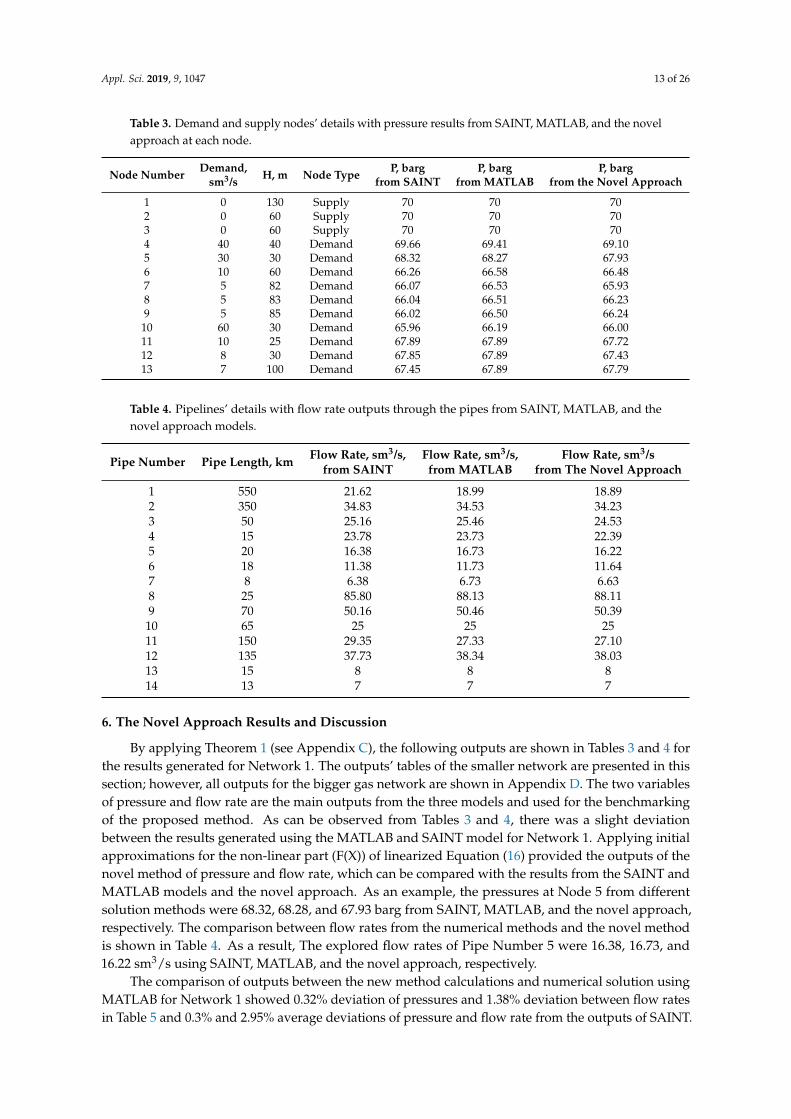
Table 3. Demand and supply nodes’ details with pressure results from SAINT, MATLAB, and the novelapproach at each node.
Node NumberDemand,
sm3/s H, m Node Type P, bargfrom SAINT
P, bargfrom MATLAB
P, bargfrom the Novel Approach
1 0 130 Supply 70 70 702 0 60 Supply 70 70 703 0 60 Supply 70 70 704 40 40 Demand 69.66 69.41 69.105 30 30 Demand 68.32 68.27 67.936 10 60 Demand 66.26 66.58 66.487 5 82 Demand 66.07 66.53 65.938 5 83 Demand 66.04 66.51 66.239 5 85 Demand 66.02 66.50 66.24
10 60 30 Demand 65.96 66.19 66.0011 10 25 Demand 67.89 67.89 67.7212 8 30 Demand 67.85 67.89 67.4313 7 100 Demand 67.45 67.89 67.79
Table 4. Pipelines’ details with flow rate outputs through the pipes from SAINT, MATLAB, and thenovel approach models.
Pipe Number Pipe Length, km Flow Rate, sm3/s,from SAINT
Flow Rate, sm3/s,from MATLAB
Flow Rate, sm3/sfrom The Novel Approach
1 550 21.62 18.99 18.892 350 34.83 34.53 34.233 50 25.16 25.46 24.534 15 23.78 23.73 22.395 20 16.38 16.73 16.226 18 11.38 11.73 11.647 8 6.38 6.73 6.638 25 85.80 88.13 88.119 70 50.16 50.46 50.39
10 65 25 25 2511 150 29.35 27.33 27.1012 135 37.73 38.34 38.0313 15 8 8 814 13 7 7 7
6. The Novel Approach Results and Discussion
By applying Theorem 1 (see Appendix C), the following outputs are shown in Tables 3 and 4 forthe results generated for Network 1. The outputs’ tables of the smaller network are presented in thissection; however, all outputs for the bigger gas network are shown in Appendix D. The two variablesof pressure and flow rate are the main outputs from the three models and used for the benchmarkingof the proposed method. As can be observed from Tables 3 and 4, there was a slight deviationbetween the results generated using the MATLAB and SAINT model for Network 1. Applying initialapproximations for the non-linear part (F(X)) of linearized Equation (16) provided the outputs of thenovel method of pressure and flow rate, which can be compared with the results from the SAINT andMATLAB models and the novel approach. As an example, the pressures at Node 5 from differentsolution methods were 68.32, 68.28, and 67.93 barg from SAINT, MATLAB, and the novel approach,respectively. The comparison between flow rates from the numerical methods and the novel methodis shown in Table 4. As a result, The explored flow rates of Pipe Number 5 were 16.38, 16.73, and16.22 sm3/s using SAINT, MATLAB, and the novel approach, respectively.
The comparison of outputs between the new method calculations and numerical solution usingMATLAB for Network 1 showed 0.32% deviation of pressures and 1.38% deviation between flow ratesin Table 5 and 0.3% and 2.95% average deviations of pressure and flow rate from the outputs of SAINT.

Appl. Sci. 2019, 9, 1047 14 of 26
Furthermore, for the bigger network with 109 nodes, the average deviations of pressure and flow ratewere 0.07% and 1.23%, respectively, using MATLAB, and the average deviations between the novelapproach and SAINT software for pressure and flow rates were 0.77% and 3.48%. The comparisonsare shown in Appendix D, Table A2. Along with accuracy, the time taken for each of the simulationswas measured for both modelled networks. The proposed new method was significantly faster, taking0.31 s, while 1 s was taken for the solution in SAINT and 2.80 for the MATLAB solution of the biggernetwork. This time is even less for the smaller network, with 0.058 s, shown in the Table 6. This methodcan be used for much bigger networks at continental scales with fast calculations.
Table 5. Deviations of the novel method from the MATLAB and SAINT outputs.
SAINT MATLABPressure
Deviation %Flow Rate
Deviation %Pressure
Deviation %Flow Rate
Deviation %13 Nodes (small network) 0.3 2.95 0.32 1.38109 Nodes (big network) 0.77 3.48 0.07 1.23
Table 6. Elapsed for calculations in seconds for each model.
Elapsed for Calculations, SecondsNovel Method MATLAB Model SAINT Model
13 Nodes (small network) 0.058 0.4 0.25109 Nodes (big network) 0.32 2.8 1
7. Conclusions
Currently, there are several numerical methods along with commercially-available softwareto solve the non-linear equations describing the compressible gas flow through the gas network.In this paper, a novel, unique mathematical method has been developed for simulating a steady-statenon-linear gas network to quantify the main characteristics, pressure and flow rate through thetransmission pipeline system.
Using two approximate models of the Irish natural gas transmission network as a casestudy the novel method was compared and benchmarked against a numerical modelling solutionusing the Newton–Raphson method carried out in MATLAB and the commercial software SAINT.The comparison of the results from all solutions showed that the new model is much faster than thealternative methods, and the average deviation between the methods was less than 0.31% (0.3% and0.32%) for pressure and less than 2.1% (2.95% and 1.38%) for flow rate. Based on these key findings,the new method can be applied as a reliable fast method to model various conditions in a gas networkeven when there is a large number of nodes and branches. The method also lends its self ideally tothe modelling of integrated energy systems as it is fast, simple, and can be easily integrated withlinear models of electrical networks. The networks presented here only contain boundary conditionsassociated with pressure for supply nodes and load for demand nodes; in reality, there may be otherreal-world constraints that impact gas supply or demand. These constraints need to be included whenmodelling real-world systems, so that in the future, the results from the novel method can be validatedwith accurate data from a real gas network.
Author Contributions: I.D.; methodology, I.D., A.E. and M.L.; software, I.D. and A.E.; formal analysis, I.D., andA.E.; original draft preparation, A.E., and M.L.; data curation, I.D., E.S. and A.E.; editing.
Funding: This work is supported by the Science Foundation Ireland, by funding Ioannis Dassios and Muyang Liuunder Investigator Programme Grant No. SFI/15/IA/3074; and Ali Ekhtiari and Eoin Syron under StrategicPartnership Programme Grant No. SFI/15/SPP/3125
Conflicts of Interest: The authors declare no conflict of interest.

Appl. Sci. 2019, 9, 1047 15 of 26
Abbreviations
The following abbreviations are used in this manuscript:
CBI Cross Border ImportCGS City Gas StationODE Ordinary Differential EquationPDE Partial Differential EquationSSM Steady-State ModelTBS Town Board StationA cross-sectional area of the pipeA matrix system of variablesD pipe inner diameterE energyf friction factorft theoretical friction factorg gravitational accelerationdh f head lossesi sender note punctuationj receiver node punctuationL nodal load (demand)l pipe lengthp nodal pressurepb basic pressurepc critical pressuredp differential pressure∆ p pressure dropU internal energyx pipeline coordinateXp pressure variable matrixXq flow rate variable matrixz elevationZ compressibility factorθ inclinationρn normal densityρ densityη pipe efficiencyτ shear stressω velocityΩ heat energyν volumeW workQ flow rateR gas constantRe Reynold’s numbert timeT TemperatureTb basic temperatureTc critical temperature

Appl. Sci. 2019, 9, 1047 16 of 26
Appendix A. Non-Linear Equations
The non-linear equations of the model are the following:
(b1,4 + 1)P24 = (1− b1,4)P2
1 − a1,4|Q1,4|Q1,4 − 2b1,4P1P4
(b1,10 + 1)P210 = (1− b1,10)P2
1 − a1,10|Q1,10|Q1,10 − 2b1,10P1P10
(1− b9,10)P29 − (1 + b9,10)P2
10 = 0 + a9,10|Q9,10|Q9,10 + 2b9,10P9P10
(1− b6,9)P26 − (1 + b6,9)P2
9 = 0 + a6,9|Q6,9|Q6,9 + 2b6,9P6P9
(1− b6,7)P26 − (1 + b6,7)P2
7 = 0 + a6,7|Q6,7|Q6,7 + 2b6,7P6P7
(1− b7,8)P27 − (1 + b7,8)P2
8 = 0 + a7,8|Q7,8|Q7,8 + 2b7,8P7P8
(1− b8,9)P28 − (1 + b8,9)P2
9 = 0 + a8,9|Q8,9|Q8,9 + 2b8,9P6P9
(b3,5 + 1)P25 = (1− b3,5)P2
3 − a3,5|Q3,5|Q3,5 − 2b3,5P3P5
(1− b5,6)P25 − (1 + b5,6)P2
6 = 0 + a5,6|Q5,6|Q5,6 + 2b5,6P5P6
(1− b5,11)P25 − (1 + b5,11)P2
11 = 0 + a5,11|Q5,11|Q5,11 + 2b5,11P5P11
(1− b4,5)P24 − (1 + b4,5)P2
5 = 0 + a4,5|Q4,5|Q4,5 + 2b4,5P4P5
(b2,4 + 1)P24 = (1− b2,4)P2
2 − a2,4|Q2,4|Q2,4 − 2b2,4P2P4
(1− b11,12)P211 − (1 + b11,12)P2
12 = 0 + a11,12|Q11,12|Q11,12 + 2b11,12P11P12
(1− b11,13)P211 − (1 + b11,13)P2
13 = 0 + a11,13|Q11,13|Q11,13 + 2b11,13P11P13
(A1)
Appl. Sci. 2019, 9, 1047 17 of 26
Appendix B. Linear Equations
The linear equations of the model are the following:
L4 = Q1,4 + Q2,4 −Q4,5
L5 = Q4,5 + Q3,5 −Q5,6 −Q5,11
L6 = Q5,6 −Q6,7 −Q6,9
L7 = Q6,7 −Q7,8
L8 = Q7,8 −Q8,9
L9 = Q8,9 + Q6,9 −Q9,10
L10 = Q9,10 + Q1,10
L11 = Q5,11 −Q11,12 −Q11,13
L12 = Q11,12
L13 = Q11,13
(A2)
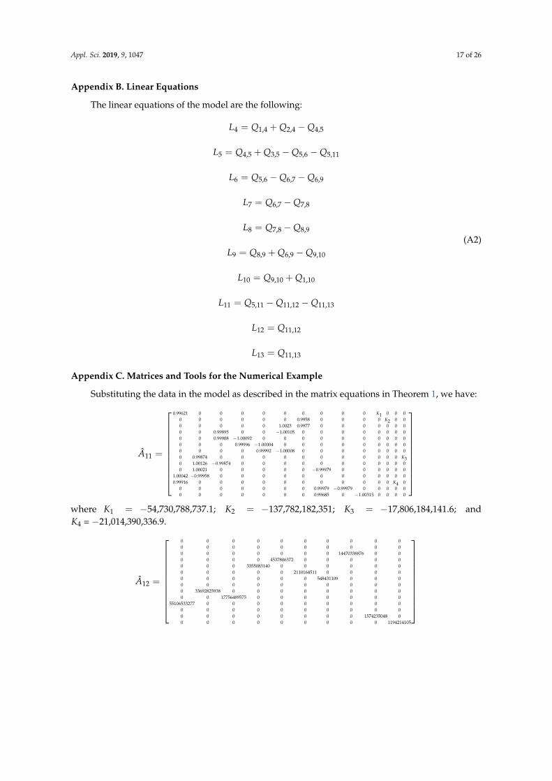
Appendix C. Matrices and Tools for the Numerical Example
Substituting the data in the model as described in the matrix equations in Theorem 1, we have:
A11 =
0.99621 0 0 0 0 0 0 0 0 0 K1 0 0 00 0 0 0 0 0 0.9958 0 0 0 0 K2 0 00 0 0 0 0 1.0023 0.9977 0 0 0 0 0 0 00 0 0.99895 0 0 −1.00105 0 0 0 0 0 0 0 00 0 0.99908 −1.00092 0 0 0 0 0 0 0 0 0 00 0 0 0.99996 −1.00004 0 0 0 0 0 0 0 0 00 0 0 0 0.99992 −1.00008 0 0 0 0 0 0 0 00 0.99874 0 0 0 0 0 0 0 0 0 0 0 K30 1.00126 −0.99874 0 0 0 0 0 0 0 0 0 0 00 1.00021 0 0 0 0 0 −0.99979 0 0 0 0 0 0
1.00042 −0.99958 0 0 0 0 0 0 0 0 0 0 0 00.99916 0 0 0 0 0 0 0 0 0 0 0 K4 0
0 0 0 0 0 0 0 0.99979 −0.99979 0 0 0 0 00 0 0 0 0 0 0 0.99685 0 −1.00315 0 0 0 0
where K1 = −54,730,788,737.1; K2 = −137,782,182,351; K3 = −17,806,184,141.6; andK4 = −21,014,390,336.9.
A12 =
0 0 0 0 0 0 0 0 0 00 0 0 0 0 0 0 0 0 00 0 0 0 0 0 0 14470338876 0 00 0 0 0 4537806372 0 0 0 0 00 0 0 3355083140 0 0 0 0 0 00 0 0 0 0 2110164511 0 0 0 00 0 0 0 0 0 548431109 0 0 00 0 0 0 0 0 0 0 0 00 33692825938 0 0 0 0 0 0 0 00 0 17756489575 0 0 0 0 0 0 0
55106533277 0 0 0 0 0 0 0 0 00 0 0 0 0 0 0 0 0 00 0 0 0 0 0 0 0 1574235048 00 0 0 0 0 0 0 0 0 1194214105

Appl. Sci. 2019, 9, 1047 18 of 26
B =
4955.28374959.1798−19.7939
9.05157.93530.34400.6876
4918.0644−11.1695−1.8961−3.9177
4912.25291.8828
28.076540.030.05.05.05.05.0
60.010.08.07.0
With the above result, we arrive at the results in Table 5.
Appendix D. Table of Outputs
Table A1. Parameters of the gas flow equation in the bigger network with 109 nodes and 112 branches.
Pipe Number From Node To Node Pipe Length,km
Diameter,m
1 1 89 75 0.92 89 88 5 0.73 89 86 150 0.74 88 87 80 0.85 87 90 70 0.86 90 91 5 0.87 86 51 70 0.78 51 52 5 0.79 51 49 20 0.710 49 50 5 0.711 49 47 10 0.712 47 48 10 0.713 47 46 15 0.714 46 45 15 0.715 45 43 10 0.716 43 44 5 0.717 43 30 10 0.718 2 41 20 0.819 41 42 10 0.7

Appl. Sci. 2019, 9, 1047 19 of 26
Table A1. Cont.
Pipe Number From Node To Node Pipe Length,km
Diameter,m
20 41 39 15 0.721 39 40 10 0.722 39 36 15 0.723 36 37 10 0.724 36 38 5 0.725 36 33 10 0.726 33 34 5 0.727 33 35 5 0.728 33 31 15 0.729 31 32 5 0.730 31 30 3 0.731 30 28 5 0.732 28 29 5 0.733 28 26 5 0.734 26 27 3 0.735 26 25 10 0.736 25 24 15 0.737 24 22 5 0.738 22 23 3 0.739 22 14 10 0.740 14 17 10 0.741 17 21 10 0.742 17 20 10 0.743 17 18 10 0.744 18 19 10 0.745 14 15 5 0.746 15 16 10 0.747 3 4 20 0.748 4 5 3 0.749 4 6 5 0.750 6 8 10 0.751 8 7 10 0.752 8 9 10 0.753 8 10 10 0.754 4 11 20 0.755 11 12 10 0.756 12 13 10 0.757 12 14 8 0.758 53 54 5 0.859 54 55 3 0.760 54 60 5 0.761 60 56 10 0.762 56 57 15 0.763 57 59 5 0.764 57 58 10 0.765 11 82 15 0.766 82 83 5 0.7

Appl. Sci. 2019, 9, 1047 20 of 26
Table A1. Cont.
Pipe Number From Node To Node Pipe Length,km
Diameter,m
67 82 84 10 0.768 84 85 10 0.769 82 78 15 0.770 78 81 5 0.771 78 79 15 0.772 79 80 15 0.773 78 76 3 0.774 76 77 3 0.775 76 75 5 0.776 75 74 10 0.777 74 73 5 0.878 73 72 5 0.779 72 71 10 0.780 71 70 5 0.781 70 69 5 0.782 72 69 5 0.783 69 68 5 0.784 68 66 5 0.785 66 67 3 0.786 73 61 10 0.787 61 62 3 0.788 62 63 3 0.789 62 64 3 0.790 62 65 3 0.791 61 60 3 0.892 61 66 2 0.793 60 55 3 0.794 90 53 5 0.895 53 92 10 0.896 92 94 10 0.897 94 95 3 0.898 92 93 3 0.799 93 97 10 0.7
100 97 98 10 0.7101 93 96 10 0.7102 91 99 20 0.7103 99 100 20 0.8104 100 101 15 0.8105 101 102 3 0.7106 101 103 5 0.8107 103 104 5 0.8108 103 105 5 0.8109 105 106 10 0.8110 106 107 5 0.8111 106 108 15 0.8112 108 109 15 0.8

Appl. Sci. 2019, 9, 1047 21 of 26
Table A2. SAINT, MATLAB, and the novel method outputs for a 109-node network.
Pressure, barg Flow Rate, sm3/sNode
NumberSAINT MATLAB Novel
ApproachPipe
NumberSAINT MATLAB Novel
Approach1 85 85 85 1 152.27 142.83 142.832 85 85 85 2 113.33 107.67 107.493 85 85 85 3 38.93 35.17 35.094 82.15 82.24 82.22 4 113.33 107.67 107.215 82.22 82.22 82.21 5 113.33 107.67 107.216 81.86 82.14 82.10 6 65.00 65.00 64.987 81.69 82.13 82.09 7 38.93 35.17 35.018 81.68 82.13 82.09 8 5.00 5.00 5.009 81.66 82.13 82.09 9 33.93 30.16 30.13
10 82.06 82.13 82.09 10 5.00 5.00 5.0011 81.23 81.16 81.11 11 28.93 25.16 25.1312 81.19 81.16 81.12 12 5.00 5.00 5.0013 80.70 81.16 81.09 13 23.93 20.16 20.0914 80.77 81.17 81.16 14 23.93 20.16 20.0015 80.84 81.17 81.13 15 23.93 20.16 20.0016 80.84 81.17 81.19 16 5.00 5.00 5.0017 80.81 81.13 81.12 17 18.93 15.16 15.1118 80.80 81.12 81.13 18 115.71 119.14 119.0019 80.77 81.12 81.12 19 5.00 5.00 5.0020 81.05 81.12 81.11 20 110.71 114.14 113.2321 81.12 81.12 81.12 21 5.00 5.00 5.0022 81.32 81.29 81.28 22 105.71 109.14 109.0123 81.32 81.29 81.29 23 5.00 5.00 5.0024 81.39 81.36 81.35 24 5.00 5.00 5.0025 81.60 81.55 81.55 25 95.71 99.14 99.0026 81.73 81.69 81.67 26 5.00 5.00 5.0027 81.73 81.69 81.68 27 2.00 2.00 2.0028 81.81 81.76 81.74 28 88.71 92.14 92.1229 81.81 81.75 81.74 29 50.00 50.00 50.0030 81.89 81.84 81.82 30 38.71 42.14 42.1231 81.92 81.87 81.80 31 57.64 57.30 57.2732 81.89 81.82 81.80 32 5.00 5.00 5.0033 82.56 82.42 82.42 33 52.64 52.30 52.0134 82.56 82.42 82.41 34 2.00 2.00 2.0035 82.56 82.42 82.41 35 50.64 50.30 50.3036 83.02 82.85 82.83 36 50.64 50.30 50.2837 83.02 82.85 82.84 37 50.64 50.30 50.2338 83.02 82.85 82.84 38 2.00 2.00 2.0039 83.86 83.60 83.60 39 48.64 48.30 48.2540 83.86 83.60 83.57 40 35.00 35.00 35.0041 84.77 84.41 84.40 41 5.00 5.00 5.0042 84.77 84.41 84.39 42 5.00 5.00 5.0043 81.95 81.85 81.79 43 5.00 5.00 5.0044 81.95 81.84 81.81 44 5.00 5.00 5.0045 81.98 81.86 81.85 45 7.00 7.00 7.0046 82.03 81.88 81.87 46 5.00 5.00 5.00

Appl. Sci. 2019, 9, 1047 22 of 26
Table A2. Cont.
Pressure, barg Flow Rate, sm3/s47 82.08 81.91 81.90 47 175.03 181.03 181.0048 82.08 81.91 81.89 48 0.00 0.00 0.0049 82.16 81.93 81.90 49 75.00 75.00 75.0050 82.16 81.93 81.90 50 15.00 15.00 15.0051 82.29 82.00 81.98 51 5.00 5.00 5.0052 82.29 82.00 81.98 52 5.00 5.00 5.0053 78.89 78.09 78.00 53 5.00 5.00 5.0054 78.87 78.09 78.00 54 100.03 106.03 106.0455 78.84 78.08 78.00 55 1.64 1.30 1.2956 78.85 78.09 78.00 56 5.00 5.00 5.0057 78.83 78.08 78.00 57 6.00 6.30 6.2058 78.97 78.08 78.09 58 42.33 36.67 36.9959 78.83 78.08 78.04 59 40.08 39.89 39.8960 78.87 78.10 78.01 60 2.25 3.23 3.2161 78.89 78.14 78.00 61 15.00 15.00 15.0062 78.88 78.14 78.01 62 15.00 15.00 15.0063 78.88 78.14 78.11 63 5.00 5.00 5.0064 78.88 78.14 78.11 64 5.00 5.00 5.0065 78.88 78.14 78.11 65 101.67 107.34 106.2366 78.89 78.15 78.09 66 2.00 2.00 2.0067 78.89 78.15 78.09 67 5.00 5.00 5.0068 78.92 78.19 78.29 68 5.00 5.00 5.0069 78.94 78.22 78.30 69 94.67 100.34 100.1270 78.94 78.22 78.19 70 5.00 5.00 5.0071 78.94 78.22 78.22 71 5.00 5.00 5.0072 78.96 78.24 78.20 72 5.00 5.00 5.0073 79.00 78.29 78.20 73 84.67 90.34 90.3274 79.09 78.41 78.39 74 2.00 2.00 2.0075 79.45 78.90 78.89 75 82.67 88.34 88.3076 79.64 79.15 79.09 76 82.67 88.34 88.3077 79.64 79.15 79.06 77 82.67 88.34 88.3078 79.79 79.30 78.93 78 38.20 40.93 40.9079 79.78 79.30 79.12 79 14.44 15.68 15.2380 79.78 79.30 79.13 80 9.44 10.68 10.0081 79.89 79.30 79.03 81 4.44 5.68 5.5282 80.49 80.18 80.00 82 23.76 25.25 24.5683 80.49 80.18 80.03 83 28.20 30.93 30.8984 80.49 80.18 80.00 84 28.20 30.93 30.8985 80.49 80.18 80.12 85 5.00 5.00 5.0086 82.90 82.32 82.29 86 44.47 47.41 47.3087 81.25 80.28 80.16 87 15.00 15.00 15.0088 83.78 82.71 82.68 88 5.00 5.00 5.0089 84.10 83.00 82.97 89 5.00 5.00 5.0090 78.96 78.09 78.09 90 5.00 5.00 5.0091 78.90 77.98 77.89 91 52.67 58.33 57.2392 78.92 78.09 78.00 92 23.20 25.93 24.5493 78.92 78.09 78.00 93 39.92 40.11 40.0194 78.92 78.09 78.03 94 48.33 42.67 42.62

Appl. Sci. 2019, 9, 1047 23 of 26
Table A2. Cont.
Pressure, barg Flow Rate, sm3/s95 78.92 78.09 78.01 95 6.00 6.00 6.0096 78.92 78.09 78.02 96 2.00 2.00 2.0097 78.92 78.09 78.02 97 2.00 2.00 2.0098 78.92 78.09 78.05 98 4.00 4.00 4.0099 78.47 77.05 77.00 99 2.00 2.00 2.00
100 78.30 76.57 76.56 100 2.00 2.00 2.00101 78.23 76.20 76.15 101 2.00 2.00 2.00102 78.12 76.17 76.16 102 65.00 65.00 65.00103 78.16 76.17 76.16 103 65.00 65.00 65.00104 78.16 76.14 76.09 104 65.00 65.00 65.00105 78.16 76.17 76.09 105 50.00 50.00 50.00106 78.16 76.16 76.18 106 15.00 15.00 15.00107 78.16 76.16 76.14 107 5.00 5.00 5.00108 78.15 76.16 76.15 108 10.00 10.00 10.00109 78.15 76.16 76.11 109 10.00 10.00 10.00
110 5.00 5.00 5.00111 5.00 5.00 5.00112 5.00 5.00 5.00
Appendix E. Figures
Figure A1. The 109-node map of Ireland’s gas network.

Appl. Sci. 2019, 9, 1047 24 of 26
References
1. Sircar, A.; Sahajpal, S.; Yadav, K. Challenges & Issues in Natural Gas Distribution Industry. STM J. 2017,7, 1–8.
2. Ekhtiari, A.; Syron, E. Moffat Constraints to supply Ireland’s Gas Network. Eng. J. (Irel. Soc. Eng.)2018. Available online: http://www.engineersjournal.ie/2018/05/15/irelands-future-natural-gas-supply-wellconnected-island/ (accessed on 1 July 2018).
3. Global, B.P. Bp Statistical Review of World Energy. 2017. Available online: http://www.bp.com/en/global/corporate/energy-economics/statistical-review-of-world-energy (accessed on 1 July 2018).
4. Gas Network Ireland. Delivering a Reliable and Secure Gas Supply. 2016. Available online: https://www.gasnetworks.ie/corporate/company/our-network/18048_GNI_GasNetwork_ReliabilityCapacity_Doc_Update.pdf (accessed on 1 July 2018).
5. Electrify. Electricity Generation in Singapore. Available online: https://electrify.sg/content/articles/electricity-generation-singapore/ (accessed on 5 November 2018).
6. Thomas, S.; Dawe, R.A. Review of ways to transport natural gas energy from countries which do not needthe gas for domestic use. Energy 2003, 28, 1461–1477. [CrossRef]
7. Jaramillo, P.; Griffin, W.M.; Matthews, H.S. Comparative life-cycle air emissions of coal, domestic natural gas,LNG, and SNG for electricity generation. Environ. Sci. Technol. 2007, 41, 6290–6296. [CrossRef] [PubMed]
8. Natgas. The Transportation of Natural Gas. Available online: http://naturalgas.org/naturalgas/transport/(accessed on 5 November 2018).
9. Ardali, E.K.; Heybatian, E. Energy regeneration in natural gas pressure reduction stations by use of gasturbo expander; evaluation of available potential in Iran. In Proceedings of the 24th World Gas Conference,Buenos Aires, Argentina, 5–9 October 2009.
10. Brandt, A.R.; Heath, G.; Kort, E.; O’sullivan, F.; P’etron, G.; Jordaan, S.; Tans, P.; Wilcox, J.; Gopstein, A.;Arent, D.; et al. Methane leaks from North American natural gas systems. Science 2014, 343, 733–735.[CrossRef]
11. Karion, A.; Sweeney, C.; P’etron, G.; Frost, G.; Hardesty, R.M.; Kofler, J.; Miller, B.R.; Newberger, T.; Wolter, S.;Banta, R. Methane emissions estimate from airborne measurements over a western United States natural gasfield. Geophys. Res. Lett. 2013, 40, 4393–4397. [CrossRef]
12. Buck, A. (Coriolis Product Manager). The Importance of Mass Flow Measurement and the Relevance ofCoriolis Technology. 2014. Available online: https://www.bronkhorst.com/blog/the-importance-of-mass-flow-measurement-and-the-relevance-of-coriolis-technology-en/ (accessed on 1 July 2018).
13. Pambour, K.A.; Bolado-Lavin, R.; Dijkema, G.P. An integrated transient model for simulating the operationof natural gas transport systems. Nat. Gas Sci. Eng. 2016, 28, 672–690. [CrossRef]
14. Wu, S.; Rios-Mercado, R.Z.; Boyd, E.A.; Scott, L.R. Model relaxations for the fuel cost minimization ofsteady-state gas pipeline networks. Math. Comput. Model. 2000, 31, 197–220. [CrossRef]
15. Askari, S.; Montazerin, N.; Zarandi, M.F. Gas networks simulation from disaggregation of low frequencynodal gas consumption. Energy 2016, 112, 1286–1298. [CrossRef]
16. Menon, E.S. Pressure Required to Transport. In Gas Pipeline Hydraulics; Forn, T.D., Hecht, M., Eds.; Taylor &Francis: New York, NY, USA, 2005; pp. 85–137, ISBN 0-8493-2785-7.
17. Carvalho, R.; Buzna, L.; Bono, F.; Guti’errez, E.; Just, W.; Arrowsmit, D. Robustness of trans-European gasnetworks. Phys. Rev. E 2009, 80, 016106. [CrossRef]
18. Szoplik, J. The Gas Transportation in a Pipeline Network. In Advances in Natural Gas Technology;Al-Megren, H., Ed.; InTech: Rijeka, Croatia, 2012; ISBN 978-953-51-0507-7.
19. Osiadacz, A.J. Simulation and Analysis of Gas Networks; Taylor & Francis: London, UK, 1987.20. DCCAE. Energy, Gas. Department of Communications, Climate Action and Environment (DCCAE). 2016.
Available online: https://www.dccae.gov.ie/en-ie/energy/topics/gas/Pages/default.aspx (accessed on1 July 2018).
21. Pambour, K.A.; Erdener, B.C.; Bolado-Lavin, R.; Dijkema, G.P. Development of a simulation framework foranalysing security of supply in integrated gas and electric power systems. Appl. Sci. 2017, 7, 47. [CrossRef]
22. Pambour, K.A.; Erdener, B.C.; Bolado-Lavin, R.; Dijkema, G.P. SAInt—A novel quasi-dynamic model forassessing security of supply in coupled gas and electricity transmission networks. Appl. Energy 2017, 203,829–857. [CrossRef]

Appl. Sci. 2019, 9, 1047 25 of 26
23. Pambour, K.A.; Erdener, B.C.; Bolado-Lavin, R.; Dijkema, G.P. An integrated simulation tool for analysingthe operation and interdependency of natural gas and electric power systems. In Proceedings of the PSIGAnnual Meeting, Vancouver, BC, Canada, 10–13 May 2016.
24. Herr’an-Gonz’alez, A.; de la Cruz, J.; de Andr’es-Toro, B.; Risco-Martin, J. Modeling and simulation of a gasdistribution pipeline network. Appl. Math. Model. 2009, 33, 1584–1600. [CrossRef]
25. Matko, D.; Geiger, G.; Gregoritza, W. Pipeline simulation techniques. Math. Comput. Simul. 2000, 52, 211–230.[CrossRef]
26. Abeysekera, M.; Wu, J.; Jenkins, N.; Rees, M. Steady state analysis of gas networks with distributed injectionof alternative gas. Appl. Energy 2016, 164, 991–1002. [CrossRef]
27. Woldeyohannes, A.D.; Majid, M.A.A. Simulation model for natural gas transmission pipeline networksystem. Simul. Model. Pract. Theory 2011, 19, 196–212. [CrossRef]
28. Woldeyohannes, A.D.; Majid, M.A.A. The accuracy and efficiency of a MATLAB-Simulink library fortransient flow simulation of gas pipelines and networks. Pet. Sci. Eng. 2010, 70, 256–265.
29. Mohring, J.; Hoffmann, J.; Halfmann, T.; Zemitis, A.; Basso, G.; Lagoni, P. Automated model reduction ofcomplex gas pipeline networks. In Proceedings of the PSIG Annual Meeting, Vancouver, BC, Canada,10–13 May 2004.
30. Van der Hoeven, T. Math in Gas and the Art of Linearization; Energy Delta Institute, Universty of Groningen:Groningen, The Netherlands, 2004; ISBN 90-367-1990-9.
31. Wu, Y.; Lai, K.K.; Liu, Y. Deterministic global optimization approach to steady-state distribution gas pipelinenetworks. Optim. Eng. 2007, 8, 259–275. [CrossRef]
32. Dassios, I.; Baleanu, D. Optimal solutions for singular linear systems of Caputo fractional differentialequations. Math. Methods Appl. Sci. 2018. [CrossRef]
33. Dassios, I.; Fountoulakis, K.; Gondzio, J. A Preconditioner for a Primal-Dual Newton Conjugate GradientsMethod for Compressed Sensing Problems. SIAM J. Sci. Comput. 2015, 37, A2783–A2812. [CrossRef]
34. Dassios, I. Optimal solutions for non-consistent singular linear systems of fractional nabla differenceequations. Circuits Syst. Signal Process. 2015, 34, 1769–1797. [CrossRef]
35. Cuffe, P.; Dassios, I.; Keane, A. Analytic Loss Minimization: A Proof. IEEE Trans. Power Syst. 2016, 31,3322–3323. [CrossRef]
36. Dassios, I. Analytic Loss Minimization: Theoretical Framework of a Second Order Optimization Method.Symmetry 2019, 11, 136. [CrossRef]
37. Dassios, I.; Cuffe, P.; Keane, A. Calculating Nodal Voltages Using the Admittance Matrix Spectrum of anElectrical Network. Mathematics 2019, 7, 106. [CrossRef]
38. Dassios, I.; Cuffe, P.; Keane, A. Visualizing Voltage Relationships Using The Unity Row Summation and RealValued Properties of the FLG Matrix. Electr. Power Syst. Res. 2016, 140, 611–618. [CrossRef]
39. Boutarfa, B.; Dassios, I. A stability result for a network of two triple junctions on the plane. Math. MethodsAppl. Sci. 2017, 40, 6076–6084. [CrossRef]
40. Dassios, I.; Jivkov, A.; Abu-Muharib, A.; James, P. A mathematical model for plasticity and damage:A discrete calculus formulation. Comput. Appl. Math. 2017, 312, 27–38. [CrossRef]
41. Dassios, I.; O’Keeffe, G.; Jivkov, A. A mathematical model for elasticity using calculus on discrete manifolds.Math. Methods Appl. Sci. 2018, 41, 9057–9070. [CrossRef]
42. Dassios, I. Stability of Bounded Dynamical Networks with Symmetry. Symmetry 2018, 10, 121. [CrossRef]43. Dassios, I. Stability of basic steady states of networks in bounded domains. Comput. Math. Appl. 2015, 70,
2177–2196. [CrossRef]44. Esqueda, H.; Herrera, R.; Botello, S.; Moreles, M.A. A geometric description of Discrete Exterior Calculus for
general. arXiv 2018, arXiv:1802.01158.45. Woldeyohannes, A.D.; Majid, M.A.A. Portfolio Implementation Risk Management Using Evolutionary
Multiobjective Optimization. Appl. Sci. 2011, 7, 1079.46. Moayeri, M. Fluid Mechanics, 3rd ed.; Shiraz University: Shiraz, Iran, 2008, ISBN 978-964-462-282-3.47. Van Wylen, G.J.; Sonntag, R.E. Fundamentals of Classical Thermodynamics; Wiley: New York, NY, USA, 2008.48. Ames, W.F. Numerical Methods for Partial Differential Equations; Elsevier: New York, NY, USA, 2014.

Appl. Sci. 2019, 9, 1047 26 of 26
49. Ramdharee, S.; Muzenda, E.; Belaid, M. A review of the equations of state and their applicability in phaseequilibrium modelling. In Proceedings of the International Conference on Chemical and EnvironmentalEngineering, New Delhi, India, 14–15 September 2013.
50. Heidaryan, E.; Salarabadi, A.; Moghadasi, J. A novel correlation approach for prediction of natural gascompressibility factor. Nat. Gas Chem. 2010, 19, 189–192. [CrossRef]
c© 2019 by the authors. Licensee MDPI, Basel, Switzerland. This article is an open accessarticle distributed under the terms and conditions of the Creative Commons Attribution(CC BY) license (http://creativecommons.org/licenses/by/4.0/).