A Non-Iterative Technique for Phase Noise

ICI Mitigation in Packet-Based OFDM

Systems

Payam Rabiei, Student Member IEEE, Won Namgoong Senior Member IEEE,

and Naofal Al-Dhahir, Fellow IEEE,

Abstract

In this paper, a practical approach for detecting packet-based orthogonal frequency division

multiplexing (OFDM) signals in the presence of phase noise is presented. An OFDM packet

consists of several OFDM symbols with full-pilot symbols at the beginning followed by consecutive

data symbols. Based on the full-pilot OFDM symbol, a frequency-domain joint phase noise and

channel vector estimator is first derived. It is shown that the phase noise vector can be estimated by

maximizing a constrained quadratic form without requiring knowledge of the channel vector. This

estimated phase noise vector is then used to compute the least squares channel estimator. Assuming

that the channel is constant during each packet, the estimated channel is used in subsequent data

OFDM symbols for equalization and data detection. Since phase noise changes from one OFDM

symbol to the next, the scattered pilots in each data OFDM symbol are used to non-iteratively

estimate and mitigate the phase noise induced interference. A significant improvement in the signal-

to-interference-plus-noise ratio is achieved using our proposed algorithms.

This work was supported in part by the National Science Foundation (NSF) under contract CCF 07-33124 and by a gift

from Research In Motion (RIM) Inc.

Index Terms

OFDM, phase noise, channel estimation, linear interpolation, scattered pilots.

I. INTRODUCTION

H IGH-rate multi-carrier transmission schemes are attractive in modern communica-

tion systems, which require broadband data transmission with high spectral effi-

ciency. However, the sensitivity of a coherent receiver to the local oscillator (LO) phase

noise increases for large signal constellation sizes. This issue becomes more pronounced

for orthogonal frequency division multiplexing (OFDM) systems [1] since the transmission

bandwidth is divided into narrower sub-channels. Moreover, as the carrier frequency increases,

the phase noise effects become more significant, potentially limiting the overall system

performance. Phase noise manifests itself in two ways [2], [3] - a common phase error

(CPE), which is an identical phase rotation in all sub-carriers, and inter-carrier interference

(ICI), which is a result of the loss of orthogonality among sub-carriers.

A. Previous Work

The effect of phase noise on the performance of OFDM systems has been extensively

analyzed (see e.g. [2], [4]–[6]) using the conventional approach of estimating the CPE term

only. Since correcting for CPE yields poor detection performance in the presence of large

phase noise, estimation and compensation of ICI caused by phase noise were considered in

[3], [7]–[9]. As ICI mitigation involves de-convolving the phase noise spectral components

from unknown data sub-carriers, the authors of [7]–[9] use an iterative algorithm for joint

data and phase noise estimation. Specifically, CPE is estimated using scattered pilots and the

data symbols are detected using the estimated CPE, after which phase noise is re-estimated

using the detected data. A common problem with iterative schemes is that they suffer from

error propagation if iteration is performed on the uncoded data, or from long latency and

high complexity if iteration is performed after the Viterbi decoder [3]. Long latency is not

practical in many packet-based systems that require fast packet acknowledgement, such as

802.11a/n. Moreover, perfect knowledge of the channel was assumed in [2], [3] during the

full-pilot OFDM symbol transmission. An approach based on joint time-domain channel and

phase noise estimation was investigated in [10] which requires an N × N matrix inversion

where N is the discrete Fourier transform (DFT) size.

B. Our Contributions

In this paper, we propose a practical approach to detect packet-based OFDM signals in the

presence of phase noise. An OFDM packet consists of several consecutive OFDM symbols

with few full-pilot symbols at the beginning which are typically used for channel estimation,

followed by data symbols in which data and pilot subcarriers are multiplexed together. We

design efficient schemes for both channel estimation during the full-pilot OFDM symbol

and data detection in subsequent data OFDM symbols with scattered pilots. In our proposed

scheme, the full-pilot OFDM symbol is used to jointly estimate the channel and phase noise

vectors. We propose a novel frequency-domain estimator in contrast to [10] which follows a

time-domain approach. The motivation to perform the estimation in the frequency domain is

the fact that the phase noise process can be well approximated by a few frequency spectral

components [4] and this property can be used to reduce the complexity of the proposed

estimation algorithm significantly.

For indoor systems such as wireless local area networks (WLAN), the channel is constant

during each OFDM packet (i.e. no mobility). However, phase noise changes from one OFDM

symbol to the next [3]. We propose to use the scattered pilots in each data OFDM symbol

to estimate the spectral components of the phase noise process in the same OFDM symbol.

Specifically, a non-iterative approach to mitigate ICI in data OFDM symbols is investigated

where the CPE terms of at least two consecutive data OFDM symbols are estimated using

their own scattered pilots. Next, the phases of the estimated CPEs are set as the phases

corresponding to the middle samples of each time-domain OFDM symbol (see Fig. 5, 6).

Interpolation between the phases of these two points provides an estimate of the phase

transition from the middle sample of the first OFDM symbol to the next. The interpolator is

derived by minimizing the mean squared error (MSE) with respect to the actual underlying

phase noise process as the cost function. We prove that, for small phase noise, a straight line

connecting the phases of the two middle points minimizes the MSE.

Our proposed approach achieves significant performance improvement compared to con-

ventional OFDM receivers with single tap per sub-carrier frequency-domain equalizers. Based

on the full-pilot OFDM symbol, our joint channel and phase noise estimator provides an

accurate channel estimate in the presence of phase noise. For data OFDM symbols, linear

phase interpolation of CPE mitigates a considerable amount of ICI. Furthermore, no iterations

are employed in the estimation process neither during the full-pilot OFDM transmission stage

nor during the data OFDM detection stage.

The rest of the paper is organized as follows. In Section II, the system model is described

and the joint frequency-domain channel and phase noise estimator is derived. In Section

III, phase noise estimation and tracking is described. In Section IV, the effective signal to

noise plus interference ratio (SINR) is analyzed and the improvement due to our proposed

algorithm is quantified. Simulation results are given in Section V and the paper is concluded

in Section VI.

II. SYSTEM MODEL AND JOINT ESTIMATOR

A. System Model and Notation

The notation of this paper is as follows. All vectors and matrices in the time-domain are

represented by a and A, respectively, while those in the frequency-domain are represented by

a and A, respectively. Unless otherwise stated, all vectors are assumed to be column vectors.

The nth element of vector a is denoted by an and the mth vector within a set of similar

vectors is denoted by am. Also, the (m,n)th element of the matrix A is denoted by A(m,n).

Furthermore, amT and amH are the transpose and Hermitian transpose of am respectively. a∗

is the complex conjugate of the scalar a. The estimate of a vector am is denoted by am.

In many packet-based OFDM systems, carrier frequency offset (CFO) synchronization and

timing synchronization are performed based on repetitive time-domain training sequences

[11], [12], [13]. In this work, we assume that the CFO and timing offset synchronization

have been determined and compensated for, based on these repetitive training sequences.

Channel estimation is performed based on full-pilot OFDM symbol following the repetitive

training sequences. One full-pilot OFDM symbol with superscript of zero (i.e. m = 0) is

assumed in this paper. If m 6= 0, that OFDM symbol is a data symbol. Since the channel

is assumed constant within the packet (i.e. no mobility), the superscript is omitted for the

channel vectors and matrices for simplicity of notation.

The signal model in the presence of phase noise is studied in [2], [14]. At the nth signal

sample of the mth OFDM symbol, phase noise introduces a random phase rotation of ejφmn

in the time-domain where φmn = φm

n−1 + ε and ε ∼ N (0, σ2ε) [2] [3] [15]. The phase noise

variance is σ2ε = 2πβTs [16] [17], where Ts is the OFDM symbol time duration and β is

the two-sided 3-dB bandwidth of the phase noise process. This effect can be expressed as

convolution1 in the frequency-domain and the received signal rmk can be written as

rmk =

N−1∑q=0

xmq hqp

m〈k−q〉 + wm

k : 0 ≤ k ≤ N − 1 (1)

where N is the OFDM symbol size, xmq for m = 0 is the qth pilot sample of the pilot vector

x0 = [x00 · · ·x0

N−1]T , hq is the qth element of the channel vector h = [h0 · · ·hN−1]

T and pmq

is the qth spectral component of the phase noise vector pm = [pm0 · · ·pm

N−1], respectively.

Note that pm is defined as a row vector. The notation 〈·〉 denotes the modulo-N operation.

Vector x0 consists of pilot tones which are known to the receiver. This vector is referred to

as the full-pilot OFDM symbol. wm is additive complex noise Gaussian distributed with zero

mean and variance σ2w. The kth phase noise spectral component of the mth OFDM symbol

pmk , can be written as [3]

pmk =

1

N

N−1∑n=0

ejφmn exp

(−j2πnk

N

): 0 ≤ k ≤ N − 1 (2)

The channel response at the kth frequency sub-carrier is given by

hk =1√N

L−1∑

l=0

hl exp

(−j2πkl

N

): 0 ≤ k ≤ N − 1 (3)

where hl is the lth tap of the time-domain channel impulse response of length L, which

is assumed to be less than the length of the cyclic prefix to maintain orthogonality among

the sub-carriers in each OFDM symbol. The channel taps are assumed to be uncorrelated

zero-mean complex Gaussian random variables with an exponential power delay profile and

variance E[|h|2] = σ2h, where E[·] is the statistical expectation operation.

1Modulo-N circular convolution because of the cyclic prefix appended at the end of each OFDM symbol.

B. Channel Estimation

Assuming that the pilot tones are drawn from a constant-modulus signal constellation,

i.e. x0qx

0∗q = Ex, the least squares (LS) estimator of the time-domain channel vector h =

[h0 · · · hL−1]T which collects the channel taps in the time-domain can be written as [18]

h = arg minh

[− log f(r0|p0T , h)]

(4)

where f(·) is the conditional probability density function (PDF) of the received vector, r0,

given the phase noise and the channel vectors. Note that Baysian estimation is not considered

in this paper which means no apriori knowledge of f(h) and f(p0T ) is available at the

receiver. Re-writing (1) in compact matrix notation, we have r0 = P 0X0Dh + w0, where

D is the N×L DFT matrix with D(n, l) = 1√N

exp (−j2πnl/N), X0 is a diagonal matrix of

pilot tones, P 0 is a column-wise circulant matrix whose first column is p0T and the following

columns are cyclically-shifted versions of it. The conditional PDF in (4) is Gaussian [18] i.e.

f(r0|p0T , h) = α exp(−‖r0 − P 0X0Dh‖2/σ2w) where α is a constant and the LS channel

estimate is derived by minimizing its exponent

h = arg minh

∥∥r0 − P 0X0Dh∥∥2

=1

Ex

DHX0HP 0Hr0

(5)

The second line in (5) is derived by differentiating the squared norm with respect to hH and

setting it to zero. Note that it can be easily shown from (2) that P 0 is an orthonormal matrix

i.e. P 0P 0H = I where I is the identity matrix. This fact has been used in derivation of the

LS channel estimate in (5). This channel estimate is a function of the unknown phase noise

matrix P 0 and, therefore, it can not be computed until P 0 is estimated beforehand. Phase

noise estimation is described in the next subsection.

C. Phase Noise Estimation

The dependence of the cost function in (4) on the channel vector can be removed by

substituting its LS estimate from (5) as follows

p0T = arg minp0T

[− log f(r0|p0T , h)]

= arg minp0T

‖r0 − 1

Ex

P 0X0DDHX0HP 0Hr0‖2

= arg minp0T

[r0Hr0 − 1

Ex

r0HP 0X0DDHX0HP 0Hr0]

= arg minp0T

[r0Hr0 − 1

Ex

r0HP 0X0

× (I −BBH)X0HP 0Hr0]

= arg maxp0T

r0HP 0X0BBHX0HP 0Hr0

= arg maxp0T

p0R0HX0BBHX0HR0p0H

= arg maxp0T

p0Mp0H

(6)

where M , R0HX0BBHX0HR0. In the definition of M , B is an N × (N − L) matrix

consisting of the last (N − L) columns of the full N × N DFT matrix and, therefore,

concatenating B with D constructs a full N ×N DFT matrix. R0 is a circulant matrix built

from the received signal vector r0.

Our objective is to solve the resulting quadratic form in (6) subject to the constraint that

all time-domain phase noise elements are small and lie in the unit circle, i.e. they are all in

the form of ejφ0n ≈ 1 + jφ0

n. Using (2) to transform this constraint to the frequency-domain,

for k = 0 we get

p00 =

1

N

N−1∑n=0

ejφ0n ≈ 1

N

N−1∑n=0

(1 + jφ0n) = 1 + j

1

N

N−1∑n=0

φ0n (7)

Therefore, a proper constraint in the frequency-domain is that the real part of p00 is 12. This

constraint follows directly from the small phase noise assumption in the time-domain.

Defining e as a 1 × N row vector with first entry equal to one and zeros otherwise, we

can formulate the proposed constraint as e × <(p0)T = 1, where <(p0) is the real part of

p0. Therefore, the constrained cost function is given by

J = p0Mp0H − λ(e×<(p0)T − 1

) (8)

where λ is a constant Lagrange multiplier.

Proposition 2.1: The solution to the constrained cost function in (8) is given by

=(p0)T = λSeT

<(p0)T = λΓ−1(ΛT S + I)eT

(9)

where Γ and Λ are the real and imaginary parts of the Hermitian matrix M , respectively,

=(p0) is the imaginary part of p0 and S ,[I +

(Γ−1Λ

)2]−1

Γ−1ΛΓ−1. The Lagrange

multiplier can be found by satisfying the constraint e×<(p0)T = 1 which gives

λ =1

e[Γ−1ΛT S + Γ−1]eT(10)

Proof: See Appendix I. ¥

The complexity of the above estimator can be reduced by considering only the most

significant elements of p0. Based on the analysis in [4], the phase noise process can be

modeled as a low-pass process and, therefore, the row vector pm can be well approximated

by estimating its Q + 1 elements only, i.e. pmN−Q/2, · · · ,pm

N−1, pm0 , · · · ,pm

Q/2. As a result,

all the matrices in the estimator of (9) can be reduced in size accordingly. The remaining

2Since this constraint is approximate, the estimated phase noise vector is biased. This bias does not cause any performance

loss since it will be averaged out during data transmission stage.

phase noise spectral components are set to zero, since they are in fact very small quantities.

Therefore, P m has a circulant and approximately banded structure with the main diagonal

equal to the CPE term and Q/2 elements above and below the main diagonal. After estimating

the real and imaginary parts of the phase noise vector in the frequency domain, the circulant

banded matrix P0

is constructed and substituted back into (5) for channel estimation. Note

that the cost function in (8) is independent of the channel. As a result, no iterations are

needed in the joint channel and phase noise estimation.

In summary, the joint estimation is performed in two steps. In the first step, Q + 1 phase

noise spectral elements are estimated using (9). In the second step, the estimated phase noise

matrix is used in (5) to compute the LS channel estimate.

III. DATA OFDM PHASE NOISE ESTIMATION

The channel estimate computed during the full-pilot OFDM symbol is used for equalization

and decoding of the data OFDM symbols. Unlike the channel response, which is assumed

constant for the duration of a packet, the phase noise matrix P m changes from one OFDM

symbol to the next. Therefore, this matrix has to be estimated for each OFDM symbol to

achieve acceptable bit error rate (BER) performance. The scattered pilots inserted in every

data OFDM symbol are used to estimate P m for m > 0.

To mitigate ICI using these scattered pilots, we propose a non-iterative interpolation-based

technique to track the random phase variations across the time-domain data samples in a given

OFDM symbol. Our proposed approach differs from all existing approaches in the literature

[3], [7]–[9] which perform joint iterative data and phase noise detection as explained in the

introduction section. We propose two phase interpolation schemes depending on whether the

receiver is able to buffer one OFDM symbol or not. In the first scheme, interpolation is

performed between the estimated CPE associated with the current data OFDM symbol and

the estimated CPE of the previous data OFDM symbol. Therefore, the receiver does not

suffer from any latency or buffering requirements.

In the second scheme, interpolation is performed based on the estimated CPEs of the

current, the previous, and the next OFDM symbols. Therefore, the actual detection of the

mth received OFDM symbol takes place after reception of the (m + 1)th OFDM symbol.

Although the performance of the second scheme is superior to the first scheme, its drawback

is the need for one OFDM symbol buffer and a latency of one OFDM symbol.

A. Interpolation Between Consecutive OFDM Symbols

Phase interpolation is performed between the CPE estimates of two consecutive OFDM

symbols. In the data OFDM symbol, we have from (1) that

rmk = pm

0 xmk hk +

N−1∑

q=0,q 6=k

xmq hqp

m〈k−q〉 + wm

k : m 6= 0 (11)

where the second term in (11) can be viewed as interference because of the unknown data.

The CPE estimate is given by [2], [7]

pm0 =

∑k rm

k h∗kx

m∗k∑

k Ex|hk|2k ∈ pilots (12)

Assuming that the cyclic prefix length is C, the estimated CPEs of the first and the second3

data OFDM symbols are interpolated into N +C intermediate points by designing a filter G,

which minimizes the MSE between the actual phase noise process and the phase-interpolating

function. This can be written as

Gopt = arg minG

E[∣∣θ − Gu

∣∣2]

= ΦθuΦ−1uu (13)

3The interpolation is performed between the first and the second data OFDM symbols for simplicity of notation and there

is no loss of generality incurred. The procedure can be easily generalized to the mth and (m + 1)th data OFDM symbols.

where u = [p10 p2

0]T and θ = [ejφ1

N/2 · · · ejφ2N/2 ]T is the actual time-domain phase noise vector

which extends from the middle point of the first data OFDM symbol to the middle point of the

second OFDM symbol. Therefore, the interpolation region starts from the sample index N/2

and ends at the sample index 3N/2 + C (see Figures 5 and 6). Φθu is the cross correlation

matrix between θ and u, Φuu is the autocorrelation matrix of u and G is an (N + C) × 2

interpolator matrix with the optimum solution Gopt, given in (13).

For a simpler solution, we propose to connect the two estimated CPE points using linear

interpolator, GL, and we prove that for small phase noise levels, Gopt reduces to GL. The

linearly approximated phase noise can be written as

θL︸︷︷︸(N+C)×1

= GL︸︷︷︸(N+C)×2

u (14)

where the nth row of GL is given by

GL(n, :) =1

N + C[3N/2 + C − n n−N/2] (15)

for N/2 ≤ n < 3N/2 + C.

Proposition 3.1: The optimum interpolation matrix Gopt between the first and the second

data OFDM symbols reduces to the linear interpolation matrix GL given in (14) if βTs ¿ 1.

Proof: See Appendix I. ¥

B. Phase Noise Tracking Strategy

The receiver with no buffer (RNB) estimates the CPE of the second received OFDM

symbol and links it to the CPE of the first symbol using matrix GL. Since GL covers only

the first half of the second symbol, the CPE is used for the samples of the second half (see

Figure 5).

Further performance improvement can be achieved if the receiver has access to memory

that allows buffering of one data OFDM symbol. The receiver with buffer (RWB) waits for

the third OFDM symbol before detecting the second OFDM symbol (see Figure 6). Hence,

RWB constructs the phase noise matrix of the second OFDM symbol, only after receiving

the third data OFDM symbol.

As an example, assuming transmission of three consecutive OFDM data symbols, the

estimated CPE points are assigned to samples N/2, 3N/2 + C and 5N/2 + 2C. The region

between the first and last CPE points (i.e., N/2 ≤ n < 5N/2 + 2C) is defined as the

interpolation region (see Figure 6). The major advantage of the RNB and RWB schemes is

their low implementation complexity. There is a significant SINR improvement by performing

the linear phase noise interpolation which will be confirmed by computer simulations in

Section V.

C. Data Detection

After the phase noise process is linearly approximated by either RNB or RWB, the data

symbol estimates are computed as follows

xmk =

Q/2∑

q=−Q/2

pm∗〈q〉r

m〈k−q〉

hk

(16)

where k ∈ data sub-carriers and m 6= 0. Basically, instead of de-rotating each OFDM sample

in the time domain, the receiver simply convolves the received signal by the estimated phase

noise spectral components followed by a simple one-tap frequency-domain equalizer (FEQ).

The convolution operation can be implemented as a matched-filter for the phase noise matrix

since P m is an orthogonal matrix. Note that the summation in (16) is only over Q + 1

elements and, therefore, it is very simple to implement. The soft output of the FEQ is passed

to the Viterbi decoder or a hard decision is made based on xmk . Both coded and uncoded bit

error rate (BER) results are given in Section V.

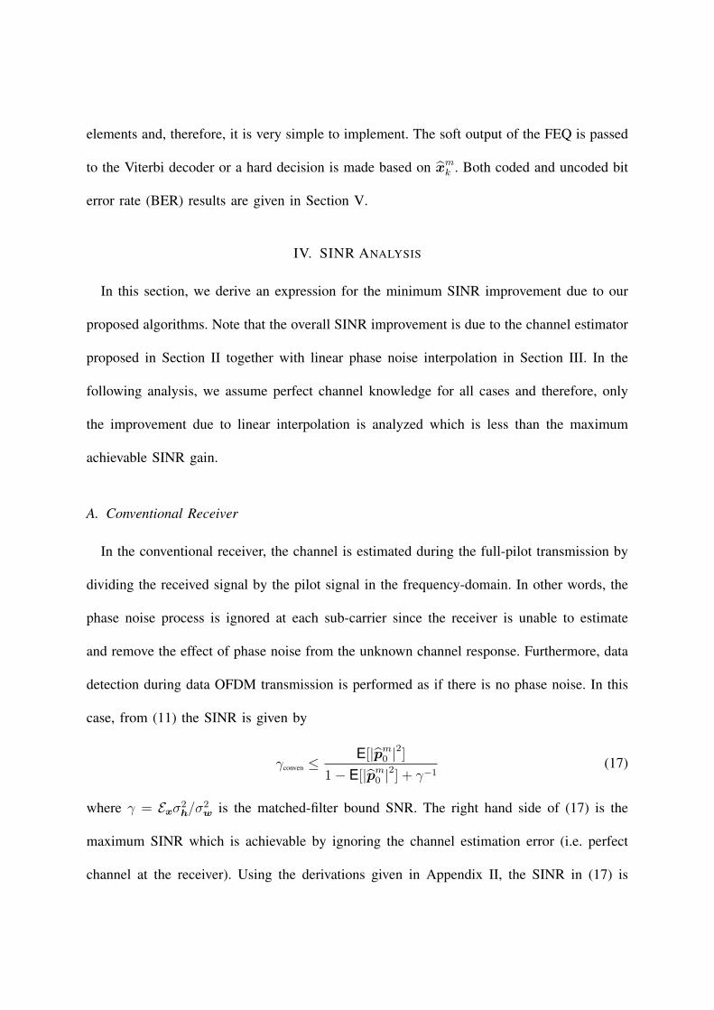
IV. SINR ANALYSIS

In this section, we derive an expression for the minimum SINR improvement due to our

proposed algorithms. Note that the overall SINR improvement is due to the channel estimator

proposed in Section II together with linear phase noise interpolation in Section III. In the

following analysis, we assume perfect channel knowledge for all cases and therefore, only

the improvement due to linear interpolation is analyzed which is less than the maximum

achievable SINR gain.

A. Conventional Receiver

In the conventional receiver, the channel is estimated during the full-pilot transmission by

dividing the received signal by the pilot signal in the frequency-domain. In other words, the

phase noise process is ignored at each sub-carrier since the receiver is unable to estimate

and remove the effect of phase noise from the unknown channel response. Furthermore, data

detection during data OFDM transmission is performed as if there is no phase noise. In this

case, from (11) the SINR is given by

γconven ≤ E[|pm0 |2]

1− E[|pm0 |2] + γ−1

(17)

where γ = Exσ2h/σ2

w is the matched-filter bound SNR. The right hand side of (17) is the

maximum SINR which is achievable by ignoring the channel estimation error (i.e. perfect

channel at the receiver). Using the derivations given in Appendix II, the SINR in (17) is

given by

γconven ≤ 1− πβNTs/3

πβNTs/3 + γ−1 $ 3

πβNTs

− 1 (18)

where $ denotes asymptotic equivalence as γ →∞.

B. Proposed Linear Phase Noise Interpolation Case

In this subsection, the effect of performing interpolation is studied and the SINR im-

provement is quantified compared to the conventional receiver. We assume that the receiver

performs the proposed RWB phase noise interpolation of Section III during the data OFDM

transmission. Assuming that the received signal in the data OFDM stage follows the model

in (1), the receiver convolves this received vector with the estimated phase noise vector in

the frequency-domain (which has already been computed using interpolation) to get

ymk =

Q/2∑

q=−Q/2

pm∗〈q〉r

m〈k−q〉 : m 6= 0

= hkxmk +

N−1∑q=0

ηm〈k−q〉hqx

mq +

N−1∑q=0

pm∗〈k−q〉w

mq

(19)

ηm in (19) is the residual phase noise vector and the interference term in (19) is a result of

phase noise estimation error. The receiver equalizes ymk by the estimated channel hk in the

frequency-domain to get the estimate of the transmitted information symbols. To simplify

the analysis, the channel estimation error is ignored. Therefore, we have

xmk =

ymk

hk

= xmk +

imk

hk

+w′mk

hk

: m 6= 0 (20)

where w′mk is the equivalent noise which is still Gaussian with the same variance as wm

k

since the frequency-domain phase noise vector pm is orthonormal and imk is the interference

which is the second term in (19). From (20), the maximum SINR can be derived as follows

γinterpolation ≤ 1N−1∑q=0

E[∣∣ηm

q

∣∣2]

+ γ−1 (21)

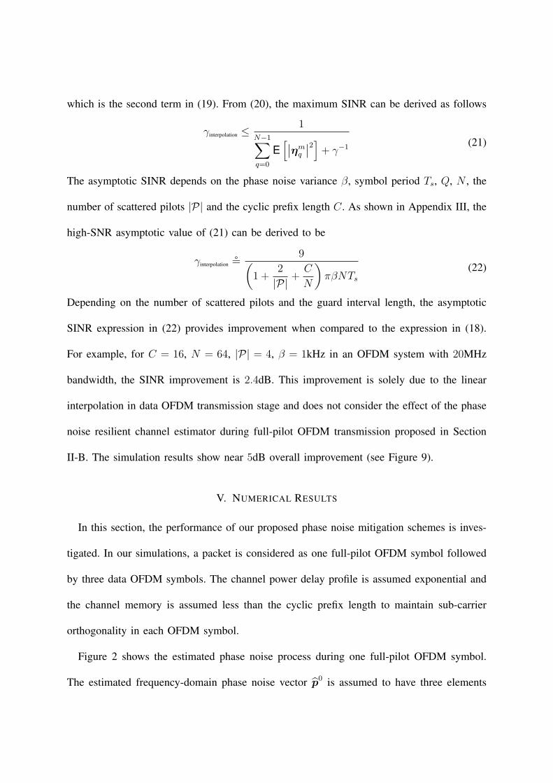
The asymptotic SINR depends on the phase noise variance β, symbol period Ts, Q, N , the

number of scattered pilots |P| and the cyclic prefix length C. As shown in Appendix III, the

high-SNR asymptotic value of (21) can be derived to be

γinterpolation $ 9(1 +

2

|P| +C

N

)πβNTs

(22)

Depending on the number of scattered pilots and the guard interval length, the asymptotic

SINR expression in (22) provides improvement when compared to the expression in (18).

For example, for C = 16, N = 64, |P| = 4, β = 1kHz in an OFDM system with 20MHz

bandwidth, the SINR improvement is 2.4dB. This improvement is solely due to the linear

interpolation in data OFDM transmission stage and does not consider the effect of the phase

noise resilient channel estimator during full-pilot OFDM transmission proposed in Section

II-B. The simulation results show near 5dB overall improvement (see Figure 9).

V. NUMERICAL RESULTS

In this section, the performance of our proposed phase noise mitigation schemes is inves-

tigated. In our simulations, a packet is considered as one full-pilot OFDM symbol followed

by three data OFDM symbols. The channel power delay profile is assumed exponential and

the channel memory is assumed less than the cyclic prefix length to maintain sub-carrier

orthogonality in each OFDM symbol.

Figure 2 shows the estimated phase noise process during one full-pilot OFDM symbol.

The estimated frequency-domain phase noise vector p0 is assumed to have three elements

denoted by p00, p0

1 and p0N−1. This implies that Q is chosen to be two in our simulation.

These three elements correspond to the three main diagonals of the circulant phase noise

matrix P0

in the frequency domain.

The MSE of the channel estimate in the presence of phase noise is compared with the

case when there is no phase noise in Figure 3. As it can be seen from the figure, the MSE

of our proposed channel estimator is close to the scheme in [10]. In our scheme, only one

super-diagonal and one sub-diagonal of P 0 are estimated, i.e. Q = 2, while the entire time-

domain phase noise vector of dimension N is estimated according to the algorithm in [10].

Also, compared to the channel estimation MSE in the conventional receiver, which ignores

the phase noise during channel estimation stage, our proposed joint channel and phase noise

scheme achieves significant performance improvement.

Figure 4 shows the channel estimation MSE as a function of Q for SNR of 30dB and

different values of β. As it can be seen from the figure, if Q = 0 (i.e. only CPE is considered),

the MSE is high. However, if we consider one sub- and one super-diagonal of P m i.e. Q = 2,

the MSE decreases significantly especially for high β. Moreover, as we further increase Q,

little improvement in the channel estimation MSE is observed. This indicates that increasing Q

to more than four results in negligible performance improvement and adds to the complexity

of the estimation algorithm.

The RNB interpolation algorithm is illustrated in Figure 5 where the phase noise process

is shown over two data OFDM symbols. The optimum interpolator together with its linear

approximation connect the two CPEs of the consecutive data OFDM symbols. As it can be

seen in this figure, CPE is used to cover the second half of the second data OFDM symbol.

Note that in this case, the receiver has no knowledge about the CPE of the next data OFDM

symbol. The RWB interpolation algorithm is also shown in Figure 6 over three data OFDM

symbols. As it can be seen in the figure, P m can be constructed only after reception of the

(m + 1)th data OFDM symbol.

Figure 7 illustrates the uncoded BER performance of the proposed channel and phase

noise estimator. The packet structure described before is used with Q = 2 and the estimated

channel is used to estimate phase noise and decode the data in the data transmission stage.

The signal constellation is assumed to be 16-QAM with normalized energy; however, pilots

are drawn from a BPSK constellation with the same average energy. The DFT size is 64 and

the number of pilots is 4 which are equi-distant in each data OFDM symbol. From Figure 7,

we observe that the performance of our proposed channel estimation method is better than

the conventional method since there is an SINR improvement in estimating the channel. The

BER performance is further improved by applying the RNB phase noise interpolation at the

receiver. Further ICI mitigation is achieved by performing RWB interpolation, as seen in

Figure 7. Moreover, the performance of the optimum interpolator is the same as the linear

interpolator for β = 1kHz and a bandwidth of 20MHz.

The coded BER performance is shown in Figure 8. The coding rate is 1/2 and the WLAN

standard convolutional encoder [133, 171] with the constraint length of 7 is used. The Viterbi

decoder uses the soft information at the output of the detector in (16) with a decoding depth

equal to five times the convolutional encoder constraint length. As it can be seen from Figure

8, our proposed algorithms result in significant performance improvements compared to the

conventional receiver.

Figure 9 shows the SINR improvement (i.e. γinterpolation/γconven) versus the matched-filter bound

SNR γ = Exσ2h/σ2

w. The overall SINR improvement is approximately 5dB. The SINR

improvement due to interpolation only is also plotted which shows good match to our

analytical results in Section IV.

VI. CONCLUSION

In this paper, we proposed a low-complexity non-iterative frequency-domain joint channel

and phase noise estimation algorithm for OFDM systems. The improved channel estimation

algorithm in the presence of phase noise enhances the performance of data detection. Addi-

tional SINR improvement is achieved by performing phase noise interpolation during data

OFDM transmission. Finally, we prove that the optimum interpolator (in the MMSE sense)

is equivalent to the linear interpolator for small values of phase noise.

APPENDIX I

PROOF OF PROPOSITION 2.1

Expanding p0 into its real and imaginary part, we can decompose the cost function as

follows

J = (<(p0) + j=(p0))M (<(p0)− j=(p0))T

− λ(e×<(p0)T − 1)

= <(p0)Γ<(p0)T + =(p0)Γ=(p0)T + 2<(p0)Λ=(p0)T

− λ(e<(p0)T − 1)

(23)

Differentiating the cost function with respect to <(p0) and =(p0) and equating to zero we

have

∂J

∂<(p0)=

[Γ<(p0)T + Λ=(p0)T

]− λeT = 0

∂J

∂=(p0)=

[Γ=(p0)T −Λ<(p0)T

]= 0

(24)

solving (24) jointly for the real and imaginary parts of phase noise vector we get

<(p0)T = Γ−1ΛT=(p0)T + λΓ−1eT

=(p0)T = Γ−1Λ<(p0)T

= Γ−1Λ[Γ−1ΛT=(p0)T + λΓ−1eT

]

= λ[I +

(Γ−1Λ

)2]−1

Γ−1ΛΓ−1eT

= λSeT

(25)

the Lagrange multiplier can be found by satisfying the constraint e<(p0)T − 1 which gives

λ =1

e[Γ−1ΛT S + Γ−1

]eT

(26)

APPENDIX II

PROOF OF PROPOSITION 3.1

As mentioned in Section III-A without loss of generality and for simplicity of notation, the

optimum interpolator between the CPE points of the first and second data OFDM symbols

in a packet is derived. To prove the theorem, we need to evaluate the autocorrelation and the

cross correlation matrices in (13). To find the autocorrelation matrix Φuu, first note that

E[ej∆φ

]= α−1

∫ ∞

−∞ej∆φ exp

(− (∆φ)2

2σ2ε |n− k|

)d∆φ

= exp

(−|n− k|σ2

ε

2

) (27)

where α =√

2πσ2ε |n− k|, ∆φ = φn − φk. Using the result in (27) to compute the expected

value of the CPE term, we get

E[p10p

1∗0 ] =

1

N2

N−1∑n=0

N−1∑

k=0

E[ejφ1ne−jφ1

k ] (28)

=1

N2

N−1∑n=0

N−1∑

k=0

exp(−|n− k|σ2ε

2)

=2(1− ξ−N) + Nξ−1 −Nξ

N2(1− ξ)(1− ξ−1)= E[p2

0p2∗0 ]

where ξ = eσ2ε/2. For small phase noise, we can use the approximation ex ≈ ∑2

i=0 (xi/i!).

Substituting these values in (28), we get E[p10p

1∗0 ] = E[p2

0p2∗0 ] ≈ 1. Similarly, we compute

E[p10p

2∗0 ] =

1

N2

N−1∑n=0

(2N+C−1)∑

k=N+C

E[ejφ1ne−jφ2

k ] (29)

=1

N2

N−1∑n=0

(2N+C−1)∑

k=N+C

exp(−|n− k|σ2ε

2)

=(1− ξN)(ξ−(N+C) − ξ−(2N+C))

N2(1− ξ)(1− ξ−1)

Applying the approximations we used previously, we have E[p10p

2∗0 ] = E[p1∗

0 p20] ≈ 1− σ2

ε

2(N+

C). Therefore, the inverse of the autocorrelation matrix Φuu can approximately be written

as

Φ−1uu ≈

1

(N + C)σ2ε

1 σ2ε

2(N + C)− 1

σ2ε

2(N + C)− 1 1

(30)

Now, the cross-correlation matrix Φθu is an (N + C) × 2 matrix which can be computed

the same way as the entries of Φuu were calculated. However, since the vector θ extends

from the second-half of the first OFDM data symbol into the guard interval and then to the

first-half of the second data symbol, i.e. the interpolation region defined in Section III-A,

and depending on the index of the vector θ, we have two different expressions for the first

column of Φθu as follows

Φθu(n, 1) = E[θ∗np10] =

1

N

N−1∑

k=0

exp(−|n− k|σ2ε

2)

=

ξ−n − 1

N(1− ξ)+

1− ξn−N

N(1− ξ−1): N/2 ≤ n < N

ξ−n − ξN−n

N(1− ξ): N ≤ n < 3N/2 + C

(31)

For both ranges of n, the two expressions in (31) converge to the same function using the

Taylor expansion of ξ. Therefore, the first column of the cross-correlation matrix can be

approximately written as

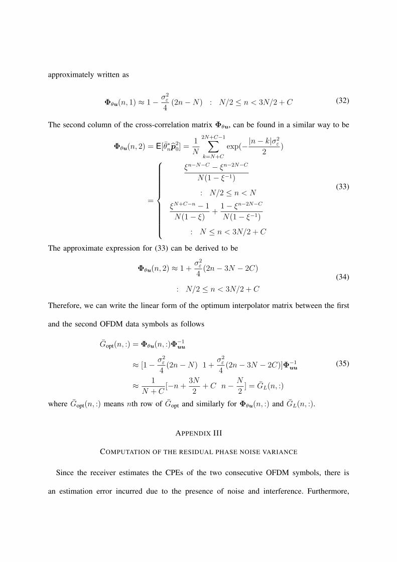
Φθu(n, 1) ≈ 1− σ2ε

4(2n−N) : N/2 ≤ n < 3N/2 + C (32)

The second column of the cross-correlation matrix Φθu, can be found in a similar way to be

Φθu(n, 2) = E[θ∗np20] =

1

N

2N+C−1∑

k=N+C

exp(−|n− k|σ2ε

2)

=

ξn−N−C − ξn−2N−C

N(1− ξ−1)

: N/2 ≤ n < N

ξN+C−n − 1

N(1− ξ)+

1− ξn−2N−C

N(1− ξ−1)

: N ≤ n < 3N/2 + C

(33)

The approximate expression for (33) can be derived to be

Φθu(n, 2) ≈ 1 +σ2

ε

4(2n− 3N − 2C)

: N/2 ≤ n < 3N/2 + C

(34)

Therefore, we can write the linear form of the optimum interpolator matrix between the first

and the second OFDM data symbols as follows

Gopt(n, :) = Φθu(n, :)Φ−1uu

≈ [1− σ2ε

4(2n−N) 1 +

σ2ε

4(2n− 3N − 2C)]Φ−1

uu

≈ 1

N + C[−n +

3N

2+ C n− N

2] = GL(n, :)

(35)

where Gopt(n, :) means nth row of Gopt and similarly for Φθu(n, :) and GL(n, :).

APPENDIX III

COMPUTATION OF THE RESIDUAL PHASE NOISE VARIANCE

Since the receiver estimates the CPEs of the two consecutive OFDM symbols, there is

an estimation error incurred due to the presence of noise and interference. Furthermore,

connecting these two points with a straight line will produce an interpolation error since the

actual underlying phase noise process is not a linear function in the index of the OFDM

samples. To compute the variance of the residual phase noise vector, it is assumed that the

initial CPE estimation error is uncorrelated with the interpolation error. Therefore, the MSE

of the frequency-domain phase noise vector estimate can be written asN−1∑q=0

E[∣∣ηm

q

∣∣2]

= Tr{

E[|pm − pm|2]}

=1

N + CTr

{E

[∣∣θ −ΦθuΦ−1uuu

∣∣2]}

=1

N + CTr

{E

[∣∣θ −ΦθuΦ−1uuug

∣∣2]}

+1

N + CTr

{E

[∣∣ΦθuΦ−1uu(ug − u)

∣∣2]}

(36)

where ug is the 2 × 1 vector containing the true values of CPEs and Tr{·} is the trace

operation. On the last line of (36), the first term on the right hand side corresponds to the

interpolation error and the second term corresponds to the CPE estimation error. For small

values of β, the expression for the optimum interpolator Gopt = ΦθuΦ−1uu can be replaced by

its linear approximation GL after which (36) is further simplified toN−1∑q=0

E[∣∣ηm

q

∣∣2]≈ 1 +

1

N + CTr

{GLΦugugG

TL

}

− 2

N + C<

[Tr

{GLΦ

Tθug

}]

+σ2

η0

N + CTr

{GLGT

L

}

(37)

We assume that the auto-correlation matrix of the true CPEs equals to the auto-correlation

matrix of the estimated ones i.e. Φugug ≈ Φuu and the cross-correlation matrix of θ and ug

is approximately equal to the cross-correlation matrix of the estimated ones i.e. Φθug ≈ Φθu.

By substituting their approximate values from (30), (32), (34) and (35) for , Φuu , Φθu and

GL, respectively, and performing some straightforward algebra, (37) is simplified to

N−1∑q=0

E[∣∣ηm

q

∣∣2]≈ πβ(N + C)Ts

9+

2

3σ2

η0(38)

The approximation in (38) assumes large OFDM symbol size i.e 1 ¿ N+C. The performance

of the CPE estimator during the data transmission stage can also be computed using (12)

which takes the average of the received signal equalized by the estimated channel at |P| pilot

positions and; therefore, the variance of the CPE estimator can be shown to be

σ2η0

=1

|P|(

πβNTs

3+

1

γ

)(39)

REFERENCES

[1] Y. G. Li and G. Stuber, “OFDM for wireless communications,” Springer, Inc, January 2006.[2] S. Wu and Y. Bar-Ness, “OFDM systems in the presence of phase noise: Consequences and solutions,” IEEE

Transactions on Communications, vol. 52, no. 11, pp. 1988–1996, November 2004.[3] D. Petrovic, W. Rave, and G. Fettweis, “Effects of phase noise on OFDM systems with and without PLL:

Characterization and compensation,” IEEE Transactions on Communications, vol. 55, no. 8, pp. 1607–1615, August2007.

[4] T. Pollet, M. Bladel, and M. Moeneclaey, “BER sensitivity of OFDM systems to carrier frequency offset and Wienerphase noise,” IEEE Transactions on Communications, vol. 43, pp. 191–193, February 1995.

[5] L. Tomba, “On the effect of Wiener phase noise in OFDM systems,” IEEE Transactions on Communications, vol. 46,pp. 580–583, May 1998.

[6] A. G. Armada and M. Calvo, “Phase noise and sub-carrier spacing effects on the performance of an OFDMcommunication system,” IEEE Communications Letters, vol. 2, pp. 11–13, Jan 1998.

[7] Q. Zou, A. Tarighat, and A. H. Sayed, “Compensation of phase noise in OFDM wireless systems,” IEEE Transactionson Signal Processing, vol. 55, no. 11, pp. 5407–5424, November 2007.

[8] S. Bittner, E. Zimmermann, and G. Fettweis, “Iterative phase noise mitigation in MIMO-OFDM systems with pilotaided channel estimation,” Vehicular Technology Conference, September 2007.

[9] J. H. Lee, J. S. Yang, S. C. Kim, and Y. W. Park, “Joint channel estimation and phase noise suppression for OFDMsystems,” Vehicular Technology Conference, May 2005.

[10] D. D. Lin, R. A. Pacheco, T. J. Lim, and D. Hatzinakos, “Joint estimation of channel response, frequency offset, andphase noise in OFDM,” IEEE Transactions on Signal Processing, vol. 54, no. 9, pp. 3542–3554, September 2006.

[11] P. H. Moose, “A technique for orthogonal frequency division multiplexing frequency offset correction,” IEEETransactions on Communications, vol. 42, pp. 2908–2914, October 1994.

[12] T. M. Schmidl and D. C. Cox, “Robust frequency and timing synchronization for OFDM,” IEEE Transactions onCommunications, vol. 45, no. 12, pp. 1613–1621, December 1997.

[13] Part 11: Wireless LAN Medium Access Control (MAC) and Physical Layer (PHY) specifications: High-speed PhysicalLayer in the 5 GHz Band, IEEE.

[14] T. C. W. Schenk, R. W. van der Hofstad, E. R. Fleddetus, and P. F. M. Smulders, “Distribution of the ICI term inphase noise impaired OFDM systems,” IEEE Transactions on Wireless Communications, vol. 6, no. 4, pp. 1488–1500,April 2007.

[15] L. Zhao and W. Namgoong, “A novel phase noise compensation scheme for communication receivers,” IEEETransactions on Communications, vol. 54, no. 3, pp. 532–542, March 2006.

[16] G. J. Foschini and G. Vannucci, “Characterizing filtered light waves corrupted by phase noise,” IEEE Transactionson Information Theory, vol. 34, no. 6, pp. 1437–1448, November 1988.

[17] A. Demir, A. Mehrotra, and J. Roychowdhury, “Phase noise in oscillators: A unifying theory and numerical methodsfor characterization,” IEEE Transactions on Circuits and Systems I, vol. 47, no. 5, pp. 655–674, May 2000.

[18] S. Kay, Fundamentals of Statistical Signal Processing. Prentice-Hall: Upper Saddle River, 1993.

Modulator

P

S

IFFT

S

P

CyclicPrefix

D/A

Lowpass

Filter

RF

Up-

Convert

Cyclic Prefix

Remove

Sampling

A/D

RF

Down-

Convert

P

S

FFT

Joint Ch.PN Est.

Lin

ea

r pha

se

no

ise in

terp

ola

tor

Ch

an

ne

l Eq

ua

lize

r

PN

de

-con

vo

lutio

n

S

P

SlicerDe-

Modulator

Cha

nn

el

nw

nje

Bit stream

Fig. 1. Block diagram of the proposed receiver

0 20 40 60 80 100 120 140−0.15

−0.1

−0.05

0

0.05

0.1

0.15

0.2

OFDM sample index

φ (r

ad)

3−tap phase noise estimateActual phase noise

Fig. 2. Phase noise estimation during preamble transmission. 3 phase noise spectral components are estimated and β = 1kHz

0 5 10 15 20 25 30 3510

−4

10−3

10−2

10−1

100

101

SNR (dB)

Cha

nnel

MS

E

Conventional β = 3kHz

Conventional β = 1kHz

Proposed β = 3kHz Q = 2

[10] β = 3kHz

Proposed β = 1kHz Q = 2

[10] β = 1kHzNo phase noise

Fig. 3. Comparison of channel estimation MSE in the presence of phase noise with the scheme in [10] and the conventionalcase for two different values of β assuming Q = 2

0 2 4 6 8 100

0.02

0.04

0.06

0.08

0.1

0.12

Q

Cha

nnel

MS

E

β = 1kHz

β = 3kHz

β = 5kHz

Fig. 4. Channel estimation MSE as a function of Q at SNR = 30dB

0 63 0 63 0−0.4

−0.2

0

0.2

0.4

0.6

0.8

1

1.2

1.4

1.6

OFDM sample index (n)

Pha

se n

oise

pro

cess

φn

Phase noiseLinear RNBOptimum RNB

arg ( p0m−1 ) arg ( p

0m )

mth symbol

(m−1)th symbol

Guard

Fig. 5. RNB phase noise interpolation algorithm for β = 3kHz. The phase of the CPE of each data OFDM symbol isused to cover the second half of the interpolation region

0 63 0 63 0 63−1.5

−1

−0.5

0

0.5

OFDM sample index (n)

Pha

se n

oise

pro

cess

φn

arg ( p0m−1 )

arg ( p0m )

mth symbol

(m−1)th symbol

arg ( p0m+1 )

(m+1)th symbol

Guard Guard

Fig. 6. RWB phase noise interpolation algorithm for β = 3kHz. The optimum and linear interpolators are shown

0 5 10 15 20 25 30 35 4010

−5

10−4

10−3

10−2

10−1

100

SNR (dB)

Unc

oded

BE

R

No phase noise and perfect CSINo phase noise and estimated CSICPE only receiverConventional receiverLinear RWB interpolatorLinear RNB interpolatorOptimum RWB interpolator

Fig. 7. Uncoded bit error rate performance of the proposed receivers with β = 1kHz and 16-QAM signal constellation

0 5 10 15 20 25 3010

−6

10−5

10−4

10−3

10−2

10−1

100

SNR (dB)

Cod

ed B

ER

Perfect phase noise and CSI

Perfect phase noise, Estimated CSI

Conventional receiver

CPE only with proposed joint CSI estimator

Linear RWB receiver

Linear RNB receiver

Fig. 8. Coded bit error rate performance of the proposed receivers with β = 1kHz and 16-QAM signal constellation

0 5 10 15 20 25 30 35 40 45 500

1

2

3

4

5

6

SNR (dB)

SIN

R im

prov

emen

t (γ in

terp

olat

ion/γ

conv

en)

(dB

)

Overall SINR improvement (simulation)Improvement due to interpolation only (simulation)Improvement due to interpolation only (Analytical)

Fig. 9. SINR improvement γinterpolation/γconven versus matched filter bound SNR. β = 1kHz