Embed Size (px)
Citation preview
University of Calgary
PRISM: University of Calgary's Digital Repository
Graduate Studies The Vault: Electronic Theses and Dissertations
2013-04-30
A New Shear Test Method for Mortar Bed Joints
Popal, Rashid
Popal, R. (2013). A New Shear Test Method for Mortar Bed Joints (Unpublished master's thesis).
University of Calgary, Calgary, AB. doi:10.11575/PRISM/24872
http://hdl.handle.net/11023/657
master thesis
University of Calgary graduate students retain copyright ownership and moral rights for their
thesis. You may use this material in any way that is permitted by the Copyright Act or through
licensing that has been assigned to the document. For uses that are not allowable under
copyright legislation or licensing, you are required to seek permission.
Downloaded from PRISM: https://prism.ucalgary.ca
UNIVERSITY OF CALGARY
A New Shear Test Method for Mortar Bed Joints
by
Rashid Popal
A THESIS
SUBMITTED TO THE FACULTY OF GRADUATE STUDIES
IN PARTIAL FULFILMENT OF THE REQUIREMENTS FOR THE
DEGREE OF MASTER OF SCIENCE
DEPARTMENT OF CIVIL ENGINEERING
CALGARY, ALBERTA
MARCH 2013
© Rashid Popal, 2013
ii
Abstract
From a review of existing test methods devised to determine the shear strength of a
mortar joint, it was concluded that among the existing methods, the triplet test is the
simplest to perform and the Hofmann & Stöckl test provides the best results in terms of
uniform stresses. The advantages of these two tests were combined in a new shear test
method designed, constructed, and utilized in this research. In the new test method,
simple equipment is used to subject a couplet to a time-dependent horizontal load as well
as to a level of normal compression stress. The couplet is placed between two rubber
sheets, two steel plates, and two roller rails to accommodate the unevenness of the
surface of the bricks, to allow smooth movement of the rollers, and to minimize the
friction between the couplet and the vertical support planes, respectively. The results of
the experimental investigation show that the developed test method produces uniform
shear stress as in the Hofmann & Stöckl test and is as simple to perform as the triplet test.
iii
Acknowledgements
I am deeply indebted to my supervisor Dr. Shelley Lissel for her continuous trust,
support, guidance, and patience throughout my research. I am grateful to Dr. Nigel Shrive
for all the valuable discussions, useful advice, and his contribution of time. I would also
like to thank my committee members Dr. Mamdouh El-Badry, Dr. Nigel Shrive, and Dr.
Sudarshan (Raj) Mehta for their time and effort in reviewing this work.
The assistance of the technical staff of the Department of Civil Engineering,
University of Calgary, during the experimental work is gratefully appreciated. Also many
thanks to Civil Department supporting staff Julie Nagy Kovacs and Chrissy Thatcher for
their support during my study time. Further, I would like to acknowledge the support of
IXL Masonry Supplies Ltd. and Spec Mix Inc. for supplying the required material for this
research. I also want to thank Dr. Andy Take from Queen’s University for providing the
Geo-PIV program. Also, many thanks to Khaled Abdelrahman for his assistance in
applying the Geo-PIV program for the data evaluation.
I am grateful to my friend Mohsen Andayesh for the valuable technical
discussions, wonderful time, and for always being there to help and support me. I am also
indebted to my mentor and friend Dr. Gerd Birkle for providing encouragement and
support from the start of this thesis to its completion. None of this would be possible
without him.
At last, but definitely not least, I would like to thank my parents for their
unconditional love and support throughout this phase of my life.
iv
To my
sister Zohal A. Popal and brother Jalil A. Popal
v
Table of Contents
Approval Page ...................................................................................................................... i
Abstract ............................................................................................................................... ii Acknowledgements ............................................................................................................ iii Table of Contents .................................................................................................................v
List of Tables .................................................................................................................... vii List of Figures and Illustrations ....................................................................................... viii
CHAPTER 1: INTRODUCTION ....................................................................................1
1.1 Objective ....................................................................................................................3 1.2 Scope and Thesis organisation ...................................................................................3
CHAPTER 2: LITERATURE REVIEW .........................................................................5
2.1 Introduction ................................................................................................................5 2.2 Existing shear test methods ........................................................................................5
2.2.1 Four unit specimens ...........................................................................................7 2.2.2 Triplet test ..........................................................................................................8 2.2.3 Couplet tests ......................................................................................................9
2.2.4 Torsion tests .....................................................................................................14 2.3 Factors affecting masonry shear strength ................................................................18
2.3.1 The effect of compressive stress ......................................................................18
2.3.2 The effect of brick and mortar properties ........................................................19
2.3.3 The effect of unit aspect ratio and load arrangement ......................................20 2.4 Mode of Failure .......................................................................................................21
2.5 Summary ..................................................................................................................21
CHAPTER 3: NUMERICAL EVALUATION ..............................................................23 3.1 Introduction ..............................................................................................................23
3.2 Material Properties ...................................................................................................23 3.3 Modelling Strategy ..................................................................................................24
3.3.1 Case Study 1 ....................................................................................................26 3.3.1.1 Triplet Test .............................................................................................27
3.3.1.2 Hofmann and Stöckl Test ......................................................................31 3.3.1.3 Proposed Test Method ...........................................................................37
3.3.2 Case Study 2 ....................................................................................................45 3.3.2.1 Hofmann and Stöckl Test ......................................................................46 3.3.2.2 Proposed Test Method ...........................................................................51
3.4 Summary ..................................................................................................................55
CHAPTER 4: EXPERIMENTAL STUDY ....................................................................57
4.1 Introduction ..............................................................................................................57 4.2 Experimental Program .............................................................................................57 4.3 Development of the Proposed Test Method ............................................................58 4.4 Materials ..................................................................................................................64
4.4.1 Brick units .......................................................................................................64
vi
4.4.2 Mortar ..............................................................................................................65
4.5 Preparation of Specimens ........................................................................................66 4.6 Measurement Equipment .........................................................................................68
4.6.1 Linear Strain Converters ..................................................................................69 4.6.2 Particle Image Velocimetry and GeoPIV ........................................................70
4.6.2.1 Preparation of Specimen for Geo-PIV ...................................................73
4.6.3 Setup of camera for the digital images ............................................................73 4.7 Summary ..................................................................................................................75
CHAPTER 5: RESULTS AND DISCUSSION .............................................................76
5.1 Introduction ..............................................................................................................76 5.2 Measurements using Linear Strain Converters ........................................................77
5.2.1 Results .............................................................................................................77
5.2.1.1 IXL-STB (Dry Pressed Brick) ...............................................................77 5.2.1.2 IPB (Extruded Brick) .............................................................................83
5.2.2 Discussion ........................................................................................................90 5.3 Measurements using GeoPIV ..................................................................................94
5.3.1 Methodology of Analysis ................................................................................95
5.3.2 Results & Discussion .......................................................................................99 5.4 Summary ................................................................................................................107
CHAPTER 6: CONCLUSIONS & RECOMMENDATIONS .....................................109
6.1 Summary ................................................................................................................109
6.2 Conclusions ............................................................................................................110 6.2.1 Finite element model .....................................................................................110
6.2.2 Experimental work ........................................................................................111 6.3 Recommendations for future work ........................................................................112
REFFERENCES ..............................................................................................................116
Appendix A: Raw data .....................................................................................................119 Appendix B: Hofmann & Stöckl test ...............................................................................128
vii
List of Tables
Table 3.1: Assumed Material Properties ........................................................................... 24
Table 3.2: Mesh refinement .............................................................................................. 25
Table 4.1: Mean compressive strength of brick units ....................................................... 65
Table 4.2: Compressive strength of mortar Type S .......................................................... 66
Table 5.1: Summary of experimental results .................................................................... 94
Table 5.2: Mean values for four rectangles selected within the mortar joint ................. 103
Table 5.3: Mean values for four rectangles encompassing the mortar joint ................... 105
viii
List of Figures and Illustrations
Figure 1.1: Orthogonally arranged masonry shear walls .................................................... 1
Figure 1.2: Mode of failures, (Lissel, 2001) ....................................................................... 2
Figure 2.1: Hamid & Drysdale Test ................................................................................... 8
Figure 2.2: Triplet Test ...................................................................................................... 9
Figure 2.3: Hofmann and Stöckl Test .............................................................................. 10
Figure 2.4: van der Pluijm Test........................................................................................ 12
Figure 2.5: Jiang/Xiao Test .............................................................................................. 13
Figure 2.6: Inclined Test .................................................................................................. 14
Figure 2.7: Samarasinghe & Lawrence test ...................................................................... 15
Figure 2.8: (a) Khalaf test, (b) Hansen & Pederson test ................................................... 16
Figure 2.9: Torsion test method (Masia, et al., 2010) ....................................................... 17
Figure 2.10: Mode of failure in a couplet ......................................................................... 21
Figure 3.1: Mesh convergence .......................................................................................... 26
Figure 3.2: Triplet test- Loading arrangement (left) and model of half triplet specimen
(right) ........................................................................................................................ 27
Figure 3.3: Case Study 1, meshing of triplet test- Model 1 (left), Model 2 (right) .......... 28
Figure 3.4: Case Study 1, .................................................................................................. 29
Figure 3.5: Case Study 1, .................................................................................................. 29
Figure 3.6: Case Study 1, stress distributions along the middle of the mortar bed joint
(Model 1), Triplet test ............................................................................................... 30
Figure 3.7: Case Study 1, stress distributions along the middle of the mortar bed joint
(Model 2), Triplet test ............................................................................................... 30
Figure 3.8: Hofmann and Stöckl Test ............................................................................... 32
Figure 3.9: Hofmann and Stöckl Test - Model 1 (left), Model 2 (right) ........................... 33
ix
Figure 3.10: Case Study 1, FE models of Hofmann and Stöckl test- Model 1 (left),
Model 2 (right) .......................................................................................................... 34
Figure 3.11: Case Study 1, normal stress distribution Model 1 (left), Model 2 (right) ... 34
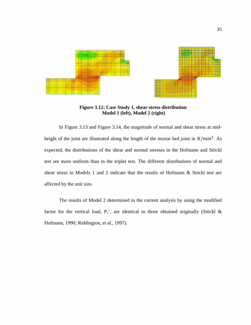
Figure 3.12: Case Study 1, shear stress distribution Model 1 (left), Model 2 (right) ...... 35
Figure 3.13: Case Study 1, stress distribution in the Hofmann and Stöckl test (Model
1) ............................................................................................................................... 36
Figure 3.14: Case Study 1, stress distribution in the Hofmann and Stöckl test (Model
2) ............................................................................................................................... 36
Figure 3.15: Case study 1, proposed test method- Model 1 (left), Model 2 (right) .......... 37
Figure 3.16: Case Study 1, finite element Model 1 and 2 of proposed test method ......... 38
Figure 3.17: Case Study 1, normal stress distribution – Model 1 (top) and 2 (bottom) ... 39
Figure 3.18: Case Study 1, shear stress distribution – Model 1 (top) and 2 (bottom) ...... 39
Figure 3.19: Case Study 1, stress distribution in the proposed test method (Model 1) ... 40
Figure 3.20: Case Study 1, stress distribution in the proposed test method (Model 2) ... 40
Figure 3.21: Case Study 1, stress distribution along the mortar bed joint in the
proposed test method (Model 1 vs. 3) ....................................................................... 43
Figure 3.22: Case Study 1, stress distribution along the mortar bed joint in the
proposed test method (Model 2 vs. 3) ....................................................................... 43
Figure 3.23: Case Study 1, stress distribution along the mortar bed joint, proposed
method (Model 4) vs. Hofmann & Stöckl (Model 2) ............................................... 44
Figure 3.24: Case Study 1, stress distribution along the mortar bed joint, proposed
method (Model 5) vs. Hofmann & Stöckl (Model 1) ............................................... 44
Figure 3.25: Vertical loads and the corresponding lever arms ......................................... 47
Figure 3.26: Case Study 2, finite element model and the corresponding deflected
shape of Hofmann & Stöckl test ............................................................................... 49
Figure 3.27: Case Study 2, normal and shear stress distribution, Hofmann & Stöckl
test ............................................................................................................................. 49
Figure 3.28: Case Study 2, stress distribution along the mortar bed joint at the mid-
height, Hofmann & Stöckl Test (Model 2) ............................................................... 50

x
Figure 3.29: Case Study 2, stress distribution along the mortar bed joint at the
interface, Hofmann & Stöckl Test (Model 2) ........................................................... 50
Figure 3.30: Case Study 2 - Finite element model of the proposed test method .............. 51
Figure 3.31: Case Study 2-Normal stress distribution of the proposed test method......... 52
Figure 3.32: Case Study 2- Shear stress distribution of the proposed test method ........... 52
Figure 3.33: Case Study 2, stress distribution along the mortar bed joint at the mid-
height, proposed test method (Model 1) ................................................................... 54
Figure 3.34: Case Study 2, stress distribution along the mortar bed joint, Proposed
Method (Model 1) vs Hofmann & Stöckl (Model 2) ................................................ 54
Figure 3.35: Case Study 2, stress distribution along the mortar bed joint at the
interface, proposed test method (Model 1) ............................................................... 55
Figure 4.1: First Version of the Proposed Test Arrangement (Popal & Lissel, 2010) ..... 59
Figure 4.2: Schematic of the new test arrangement (version 2) ....................................... 61
Figure 4.3: Test arrangement for version 2 of the proposed test method ......................... 62
Figure 4.4: IXL Sable Titans Brick, left, and Interstate Platinum Brick, right ................. 64
Figure 4.5: Masonry specimens, left (IXL-STB) and right (IPB) ..................................... 67
Figure 4.6: The simple jig for constructing the couplets .................................................. 67
Figure 4.7: Arrangement of LSCs on the specimens ........................................................ 70
Figure 4.8: Principles of PIV analysis (White & Take, 2002) .......................................... 71
Figure 4.9: GeoPIV image processing system (White & Take, 2002) ............................. 72
Figure 4.10: Painted specimen, left, speckled specimen, right ......................................... 73
Figure 4.11: Camera and Light setup (left); the actual field of view (right) .................... 74
Figure 5.1: Typical cracks observed for Series # I through IV ......................................... 78
Figure 5.2: Results for Series # I, = 0.03 N/mm2 .......................................................... 79
Figure 5.3: Results for Series # II, = 0.25 N/mm2 ......................................................... 81
Figure 5.4: Results for Series # III, = 0.375 N/mm2...................................................... 82
xi
Figure 5.5: Results for Series # IV, = 0.50 N/mm2 ....................................................... 83
Figure 5.6: Typical cracks observed for Series # V through VIII .................................... 84
Figure 5.7: Results for Series # V, = 0.03 N/mm2 ......................................................... 85
Figure 5.8: Results for Series # VI, = 0.25 N/ mm2 ...................................................... 87
Figure 5.9: Results for Series # VII, = 0.375 N/mm2 .................................................... 88
Figure 5.10: Results for Series # VIII, = 0.50 N/mm2 ................................................... 89
Figure 5.11: Moment and stress concentration due to eccentrically applied load ............ 91
Figure 5.12: Test specimens ............................................................................................. 91
Figure 5.13: Stress concentration around the holes due to the mortar cylinders .............. 92
Figure 5.14: Typical example for the observed brick failure ............................................ 93
Figure 5.15: Meshed patches ............................................................................................ 96
Figure 5.16: Comparison of LSC and Digital GeoPIV Displacement Measurements
for Specimen # 2 in Series IA ................................................................................... 97
Figure 5.17: Rectangles used for shear strain calculations .............................................. 98
Figure 5.18: Shear strain ................................................................................................... 98
Figure 5.19: Typical displaced versus initial patches for Specimen 2 in Series IA ........ 107
Figure 6.1: Suggested modifications to as is-state of the test setup................................ 115
1
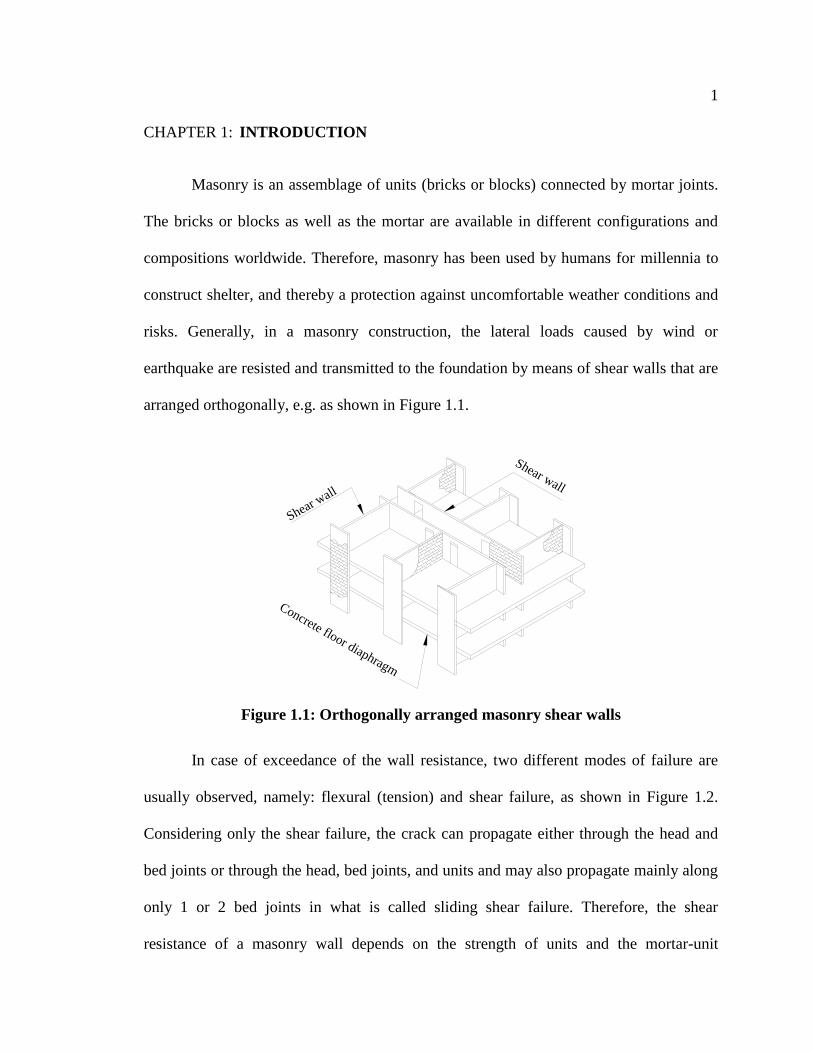
CHAPTER 1: INTRODUCTION
Masonry is an assemblage of units (bricks or blocks) connected by mortar joints.
The bricks or blocks as well as the mortar are available in different configurations and
compositions worldwide. Therefore, masonry has been used by humans for millennia to
construct shelter, and thereby a protection against uncomfortable weather conditions and
risks. Generally, in a masonry construction, the lateral loads caused by wind or
earthquake are resisted and transmitted to the foundation by means of shear walls that are
arranged orthogonally, e.g. as shown in Figure 1.1.
Figure 1.1: Orthogonally arranged masonry shear walls
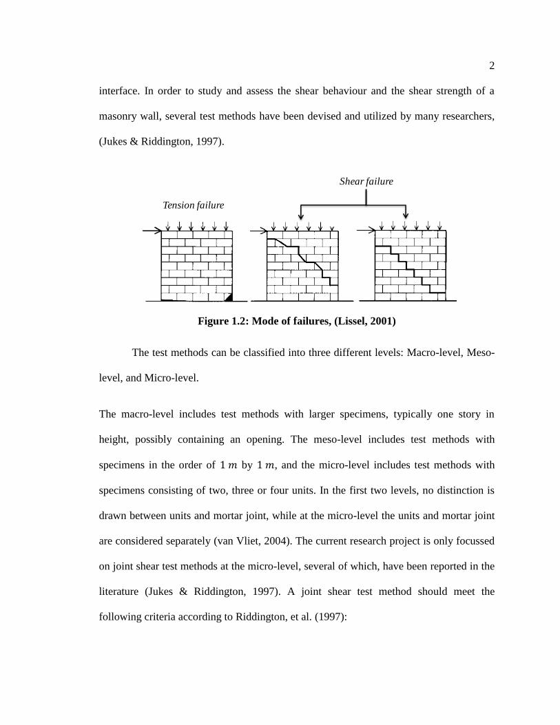
In case of exceedance of the wall resistance, two different modes of failure are
usually observed, namely: flexural (tension) and shear failure, as shown in Figure 1.2.
Considering only the shear failure, the crack can propagate either through the head and
bed joints or through the head, bed joints, and units and may also propagate mainly along
only 1 or 2 bed joints in what is called sliding shear failure. Therefore, the shear
resistance of a masonry wall depends on the strength of units and the mortar-unit
Shear wall
Shear wall
Concrete floor diaphragm
2
interface. In order to study and assess the shear behaviour and the shear strength of a
masonry wall, several test methods have been devised and utilized by many researchers,
(Jukes & Riddington, 1997).
Figure 1.2: Mode of failures, (Lissel, 2001)
The test methods can be classified into three different levels: Macro-level, Meso-
level, and Micro-level.
The macro-level includes test methods with larger specimens, typically one story in
height, possibly containing an opening. The meso-level includes test methods with
specimens in the order of by , and the micro-level includes test methods with
specimens consisting of two, three or four units. In the first two levels, no distinction is
drawn between units and mortar joint, while at the micro-level the units and mortar joint
are considered separately (van Vliet, 2004). The current research project is only focussed
on joint shear test methods at the micro-level, several of which, have been reported in the
literature (Jukes & Riddington, 1997). A joint shear test method should meet the
following criteria according to Riddington, et al. (1997):
Shear failure
Tension failure
3
The normal and shear stress distribution should be uniform.
Majority of the joint should be close to failure when failure is initiated at
one point.
No tensile stresses should be induced along the joint that could affect the
failure load.
The failure should be initiated away from the edge of a joint.
The complexity needed to carry out the test should be as simple as
possible.
1.1 Objective
The objective of this research is to devise a simple test method that produces
uniform shear stress in the mortar bed joint and meets the criteria listed above. It is not
intended to evaluate the shear strength of mortar bed joints.
To achieve this objective, a simple finite element analysis of two existing
methods and of the devised test method was performed to gain insight into the state of
stress imposed in the bed joint. Subsequently, an experimental program using two types
of bricks combined with only one type of mortar was conducted to evaluate the devised
test arrangement.
1.2 Scope and Thesis organisation
In Chapter 2, a literature review of test methods at the micro-level is presented.
Furthermore, some of the factors affecting the shear strength of a masonry wall are
discussed. From the literature review, two test methods are identified that meet most of
the above criteria: the Hofmann & Stöckl and the Triplet tests. While the Hofmann &
4
Stöckl test produces the most uniformly distributed normal and shear stresses along the
bed joint, it requires very complex equipment, (Stöckl & Hofmann, 1990). The triplet test
is much simpler, but does not produce the ideal normal and shear stress distributions
(Jukes & Riddington, 1997; Riddington, et al., 1997). While the Hofmann & Stöckl test
produces the best results and the triplet test is simpler to perform, the challenge remains
to devise a test method that is able to combine the advantages of both test methods
In Chapter 3, the Hofmann & Stöckl test and the triplet test are evaluated and
compared based on a two-dimensional finite element analysis assuming linear stress-
strain behaviour of the material. Subsequently, a new joint shear test method is proposed
for specimens consisting of two units connected by a mortar joint over the entire length in
stack bond. Numerical analysis of the new test method is also carried out using finite
element method (FEM) for comparison with the Hofmann & Stöckl and triplet tests. In
Chapter 4, an experimental program using the new test method is described. In addition,
a short description of the measurement systems utilized is included. Linear strain
converters (LSCs) are used to prove the reproducibility of the new test method by
determining the variation in load-displacement behaviour. A Particle Image Velocimetry
measurement system (GeoPIV) is used to gain insight into the state of stress imposed in
the bed joint in the new test method.
In Chapter 5, the experimental data obtained using LSCs and the GeoPIV
measurement system are evaluated and discussed. The performance of the new test
method is evaluated on the basis of these data. In Chapter 6, the research presented in this
thesis is summarized, followed by conclusions and recommendations for future work.
5
CHAPTER 2: LITERATURE REVIEW
2.1 Introduction
Within the scope of this research, the existing joint shear test methods at the
micro-level are reviewed and discussed. The discussion is primarily concentrated on the
test methods that provide bending moment free testing of the mortar bed joint, and on the
methods that are simpler to perform. While the test methods are discussed, the criteria, as
specified in Chapter 1, are taken into account. The existing test methods are summarized
and discussed to distinguish their respective advantages and disadvantages. For this
purpose, test methods are ordered by the number of units of the specimens, and the type
of applied shearing load. Beyond that, factors having an effect on the results of bond
shear strength of a mortar joint are emphasized and reviewed. The knowledge gained will
be used to devise a new test method that is able to combine the advantages of the existing
test methods.
2.2 Existing shear test methods
A review of the literature reveals that many researchers have utilized different
methods to measure the shear strength of a mortar bed joint at the micro level, (Jukes &
Riddington, 1997). The existing test methods differ either in their arrangement or in the
type of specimen. Considering the test arrangement, the differences are mainly in the load
arrangement and application. For example, in some of the tests, the specimen is only
subjected to a horizontal load (i.e. the line of action of the load is acting parallel to the
mortar joint), and in others the specimen is subjected to a horizontal as well as a vertical
load (i.e. the mortar joint is subjected to parallel und normal stress). In addition to these
6
two types of load application, there exist test methods in which the specimen is subjected
to a torque with or without a normal compressive stress. With respect to the specimens,
the test methods differ from each other in the number of units and shape of the
specimens. In most of the existing test methods, a couplet (two-unit specimen) is utilized
to measure the shear strength of a mortar joint, but there also exist test methods which are
performed using four or three-unit specimens. For example, a four-unit specimen was
used by Hamid & Drysdale, (Hamid, et al., 1979), and a triplet is suggested by the
European Committee for Standardization (CEN) to measure the shear strength of a mortar
joint, (DIN EN 1052-3, 2007). Generally, couplets are subjected either to shearing force
or to torsion, while triplets (three-unit specimen) and four-unit specimens are subjected
only to shearing force.
However, regardless of the number of units or the shape of the specimens, it is
quite a challenge in practice to apply load to a specimen without inducing bending
moment to the mortar bed joint. This is a result of the eccentricity that exists between the
line of action of the applied shearing load and the center line of the mortar bed joint. In
order to reduce or to eliminate the induced bending moment, researchers have utilized a
combination of horizontal and vertical load, or a specific manner of load application, or a
particular load and support arrangement. For example, Hofmann & Stöckl (1986) utilized
a combination of horizontal and vertical load, van der Pluijm (1993) utilized a specific
way of load application, and Jiang & Xiao (1994)
used both the load and support
condition to perform a shear test free of bending moment. Furthermore, to avoid inducing
bending moment in the mortar joint, researchers have devised test methods in which a
7
couplet is subjected to a torque to determine the bond shear strength of a mortar joint
(Samarasinghe & Lawrence, 1994; Khalaf, 1995; Hansen & Pedersen, 2008; Hansen &
Pedersen, 2009; Masia, et al., 2010). However, results obtained using these test methods,
in which the specimen is subjected to a torque, represent the torsional shear capacity of
masonry subjected to flexural about the axis normal to the bed joints, (Samarasinghe &
Lawrence, 1994).
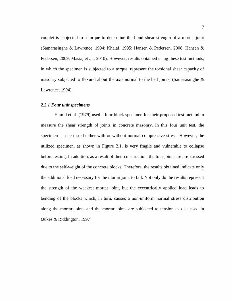
2.2.1 Four unit specimens
Hamid et al. (1979) used a four-block specimen for their proposed test method to
measure the shear strength of joints in concrete masonry. In this four unit test, the
specimen can be tested either with or without normal compressive stress. However, the
utilized specimen, as shown in Figure 2.1, is very fragile and vulnerable to collapse
before testing. In addition, as a result of their construction, the four joints are pre-stressed
due to the self-weight of the concrete blocks. Therefore, the results obtained indicate only
the additional load necessary for the mortar joint to fail. Not only do the results represent
the strength of the weakest mortar joint, but the eccentrically applied load leads to
bending of the blocks which, in turn, causes a non-uniform normal stress distribution
along the mortar joints and the mortar joints are subjected to tension as discussed in
(Jukes & Riddington, 1997).
8
Figure 2.1: Hamid & Drysdale Test
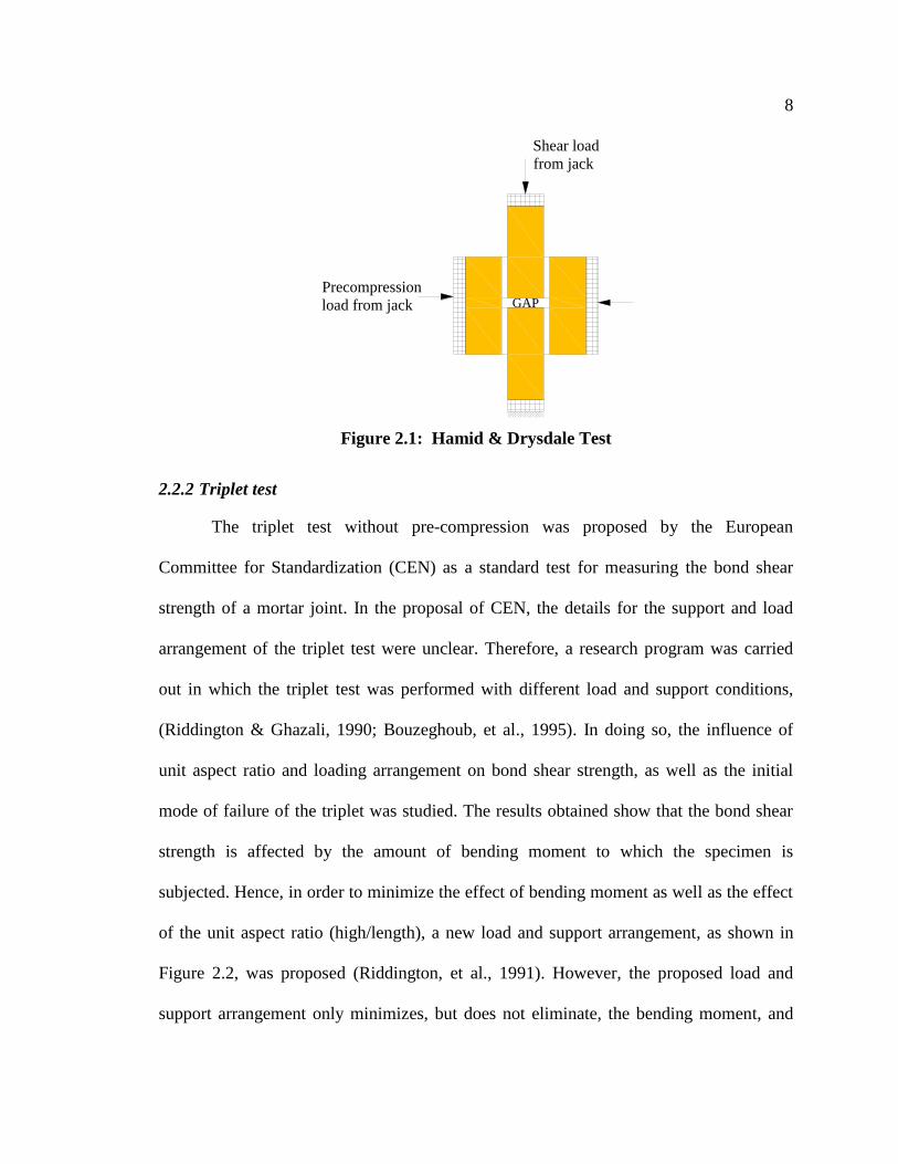
2.2.2 Triplet test
The triplet test without pre-compression was proposed by the European
Committee for Standardization (CEN) as a standard test for measuring the bond shear
strength of a mortar joint. In the proposal of CEN, the details for the support and load
arrangement of the triplet test were unclear. Therefore, a research program was carried
out in which the triplet test was performed with different load and support conditions,
(Riddington & Ghazali, 1990; Bouzeghoub, et al., 1995). In doing so, the influence of
unit aspect ratio and loading arrangement on bond shear strength, as well as the initial
mode of failure of the triplet was studied. The results obtained show that the bond shear
strength is affected by the amount of bending moment to which the specimen is
subjected. Hence, in order to minimize the effect of bending moment as well as the effect
of the unit aspect ratio (high/length), a new load and support arrangement, as shown in
Figure 2.2, was proposed (Riddington, et al., 1991). However, the proposed load and
support arrangement only minimizes, but does not eliminate, the bending moment, and
Precompression
load from jack
Shear load
from jack
GAP
9
for this reason as long as the triplet test is conducted without pre-compression, most of
the mortar joint will be subjected to a considerable amount of normal tensile stress,
(Riddington, et al., 1997) and (Popal & Lissel, 2010). In addition, as was the case with
the four unit test, the results obtained represent only the shear strength of the weakest
mortar joint of the specimen, and both of these test methods require more material
compared to tests using a two unit specimen (couplet). Advantages of the triplet test
include the symmetrical nature of the specimen and the load arrangement, since this
facilitates a stable load arrangement in comparison to the couplet (Jukes & Riddington,
1997), and in addition, the test is feasible with simple equipment.
Figure 2.2: Triplet Test
2.2.3 Couplet tests
As mentioned previously, the aim is to devise a test setup that reduces or ideally
eliminates the effect of bending moment. Keeping this in mind, one existing test
arrangement that measures the shear strength of a mortar joint free from the effect of
bending moment was proposed by Hofmann & Stöckl (1986). In this test method, a
F/2
F
F/2
e = L/15
e = L/15
L
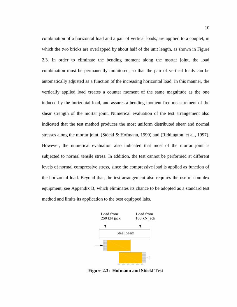
10
combination of a horizontal load and a pair of vertical loads, are applied to a couplet, in
which the two bricks are overlapped by about half of the unit length, as shown in Figure
2.3. In order to eliminate the bending moment along the mortar joint, the load
combination must be permanently monitored, so that the pair of vertical loads can be
automatically adjusted as a function of the increasing horizontal load. In this manner, the
vertically applied load creates a counter moment of the same magnitude as the one
induced by the horizontal load, and assures a bending moment free measurement of the
shear strength of the mortar joint. Numerical evaluation of the test arrangement also
indicated that the test method produces the most uniform distributed shear and normal
stresses along the mortar joint, (Stöckl & Hofmann, 1990) and (Riddington, et al., 1997).
However, the numerical evaluation also indicated that most of the mortar joint is
subjected to normal tensile stress. In addition, the test cannot be performed at different
levels of normal compressive stress, since the compressive load is applied as function of
the horizontal load. Beyond that, the test arrangement also requires the use of complex
equipment, see Appendix B, which eliminates its chance to be adopted as a standard test
method and limits its application to the best equipped labs.
Figure 2.3: Hofmann and Stöckl Test
Load from
250 kN jack
Load from
100 kN jack
Steel beam
11
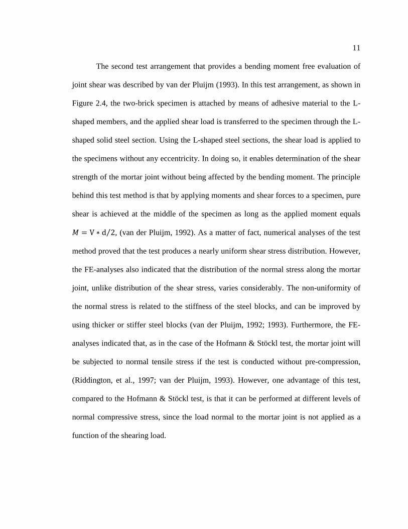
The second test arrangement that provides a bending moment free evaluation of
joint shear was described by van der Pluijm (1993). In this test arrangement, as shown in
Figure 2.4, the two-brick specimen is attached by means of adhesive material to the L-
shaped members, and the applied shear load is transferred to the specimen through the L-
shaped solid steel section. Using the L-shaped steel sections, the shear load is applied to
the specimens without any eccentricity. In doing so, it enables determination of the shear
strength of the mortar joint without being affected by the bending moment. The principle
behind this test method is that by applying moments and shear forces to a specimen, pure
shear is achieved at the middle of the specimen as long as the applied moment equals
⁄ , (van der Pluijm, 1992). As a matter of fact, numerical analyses of the test
method proved that the test produces a nearly uniform shear stress distribution. However,
the FE-analyses also indicated that the distribution of the normal stress along the mortar
joint, unlike distribution of the shear stress, varies considerably. The non-uniformity of
the normal stress is related to the stiffness of the steel blocks, and can be improved by
using thicker or stiffer steel blocks (van der Pluijm, 1992; 1993). Furthermore, the FE-
analyses indicated that, as in the case of the Hofmann & Stöckl test, the mortar joint will
be subjected to normal tensile stress if the test is conducted without pre-compression,
(Riddington, et al., 1997; van der Pluijm, 1993). However, one advantage of this test,
compared to the Hofmann & Stöckl test, is that it can be performed at different levels of
normal compressive stress, since the load normal to the mortar joint is not applied as a
function of the shearing load.
12
Figure 2.4: van der Pluijm Test
The test method described by Jiang & Xiao (1994) is also one in which the load
and support arrangements are utilized in combination to produce a bending moment free
shear test. As shown in Figure 2.5, the couplet is bracketed between two T-sections, and
is placed in the midspan of a beam. The applied loads (at B and C) and supports of the
beam (at A and D) create a constant shear force between points B and C, and a moment
that equals zero in the middle of the mortar joint. The finite element analysis, presented
by Jiang & Xiao, showed a uniform distribution of shear stress along the mortar joint, but
stresses normal to the mortar joint were not reported. Furthermore, the test method only
provides results for the initial bond shear strength, , while the ultimate shear strength of
a masonry assemblage, , is expected to be a function of the initial bond shear strength,
the internal coefficient of friction ( ) at the interface, and the normal stress due to
gravity. However, this test method can be combined with a simple test apparatus
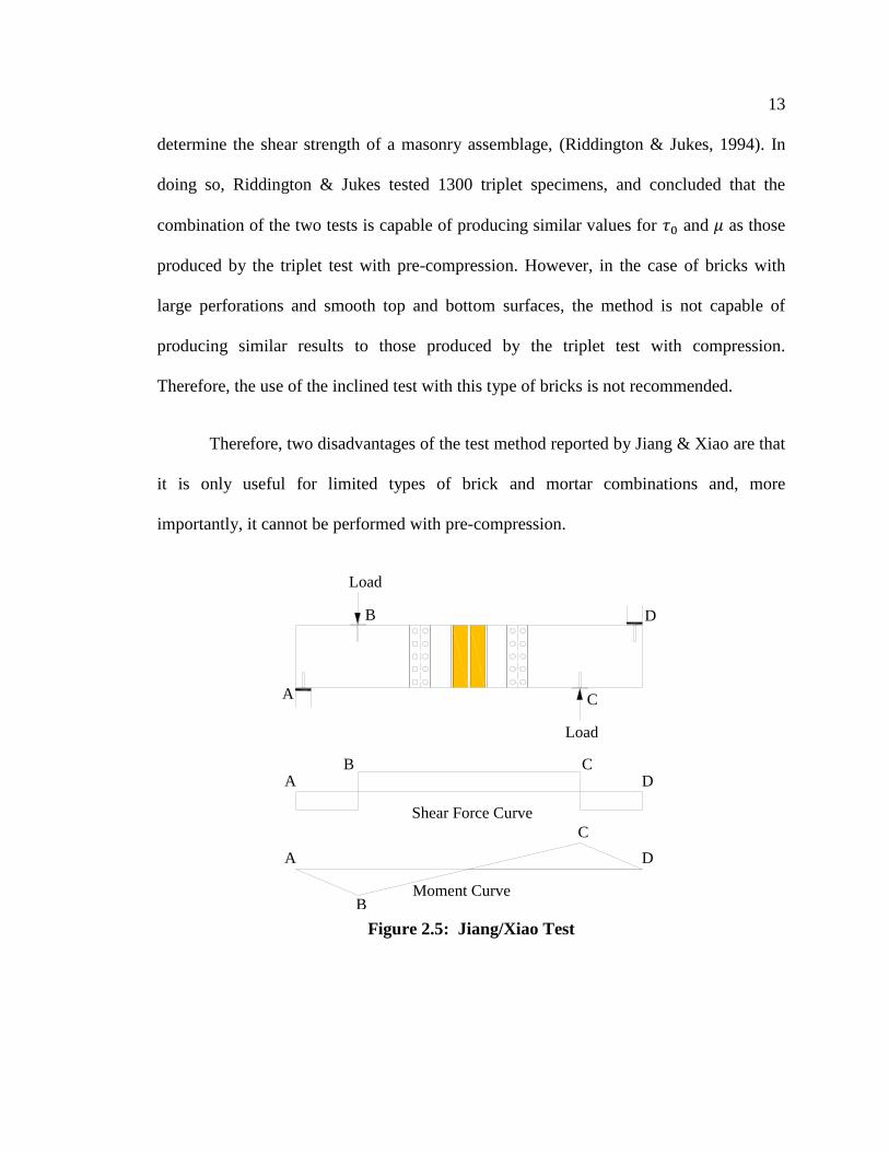
proposed by Ghazali & Riddington (1988) to obtain the ultimate shear strength.
The simple apparatus, as shown in Figure 2.6, is intended for measuring the
coefficient of friction and was combined with the triplet test without pre-compression, to
Load from
jack
Load
fro
m j
ack
M
V M
V
d
M = V*d/2
V
13
determine the shear strength of a masonry assemblage, (Riddington & Jukes, 1994). In
doing so, Riddington & Jukes tested 1300 triplet specimens, and concluded that the
combination of the two tests is capable of producing similar values for and as those
produced by the triplet test with pre-compression. However, in the case of bricks with
large perforations and smooth top and bottom surfaces, the method is not capable of
producing similar results to those produced by the triplet test with compression.
Therefore, the use of the inclined test with this type of bricks is not recommended.
Therefore, two disadvantages of the test method reported by Jiang & Xiao are that
it is only useful for limited types of brick and mortar combinations and, more
importantly, it cannot be performed with pre-compression.
Figure 2.5: Jiang/Xiao Test
Load
Load
A
B
C
D
AB C
D
A D
B
C
Shear Force Curve
Moment Curve
14
Figure 2.6: Inclined Test
2.2.4 Torsion tests
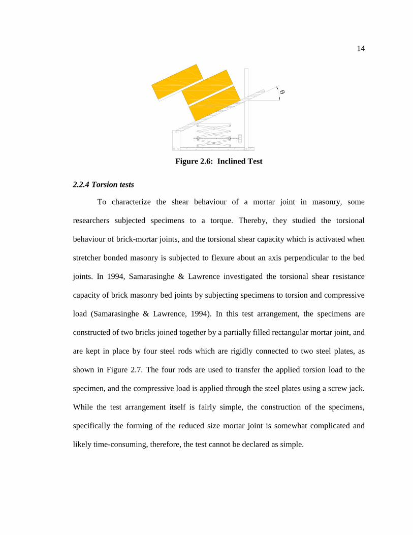
To characterize the shear behaviour of a mortar joint in masonry, some
researchers subjected specimens to a torque. Thereby, they studied the torsional
behaviour of brick-mortar joints, and the torsional shear capacity which is activated when
stretcher bonded masonry is subjected to flexure about an axis perpendicular to the bed
joints. In 1994, Samarasinghe & Lawrence investigated the torsional shear resistance
capacity of brick masonry bed joints by subjecting specimens to torsion and compressive
load (Samarasinghe & Lawrence, 1994). In this test arrangement, the specimens are
constructed of two bricks joined together by a partially filled rectangular mortar joint, and
are kept in place by four steel rods which are rigidly connected to two steel plates, as
shown in Figure 2.7. The four rods are used to transfer the applied torsion load to the
specimen, and the compressive load is applied through the steel plates using a screw jack.
While the test arrangement itself is fairly simple, the construction of the specimens,
specifically the forming of the reduced size mortar joint is somewhat complicated and
likely time-consuming, therefore, the test cannot be declared as simple.
15
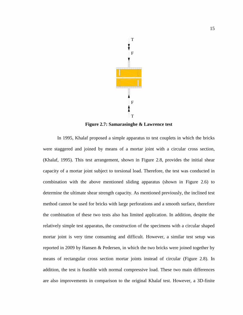
Figure 2.7: Samarasinghe & Lawrence test
In 1995, Khalaf proposed a simple apparatus to test couplets in which the bricks
were staggered and joined by means of a mortar joint with a circular cross section,
(Khalaf, 1995). This test arrangement, shown in Figure 2.8, provides the initial shear
capacity of a mortar joint subject to torsional load. Therefore, the test was conducted in
combination with the above mentioned sliding apparatus (shown in Figure 2.6) to
determine the ultimate shear strength capacity. As mentioned previously, the inclined test
method cannot be used for bricks with large perforations and a smooth surface, therefore
the combination of these two tests also has limited application. In addition, despite the
relatively simple test apparatus, the construction of the specimens with a circular shaped
mortar joint is very time consuming and difficult. However, a similar test setup was
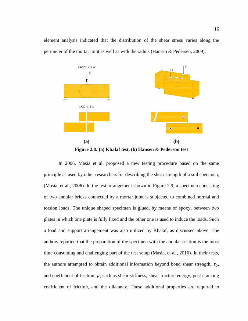
reported in 2009 by Hansen & Pedersen, in which the two bricks were joined together by
means of rectangular cross section mortar joints instead of circular (Figure 2.8). In
addition, the test is feasible with normal compressive load. These two main differences
are also improvements in comparison to the original Khalaf test. However, a 3D-finite
F
T
F
T
16
element analysis indicated that the distribution of the shear stress varies along the
perimeter of the mortar joint as well as with the radius (Hansen & Pedersen, 2009).
(a)
(b)
Figure 2.8: (a) Khalaf test, (b) Hansen & Pederson test
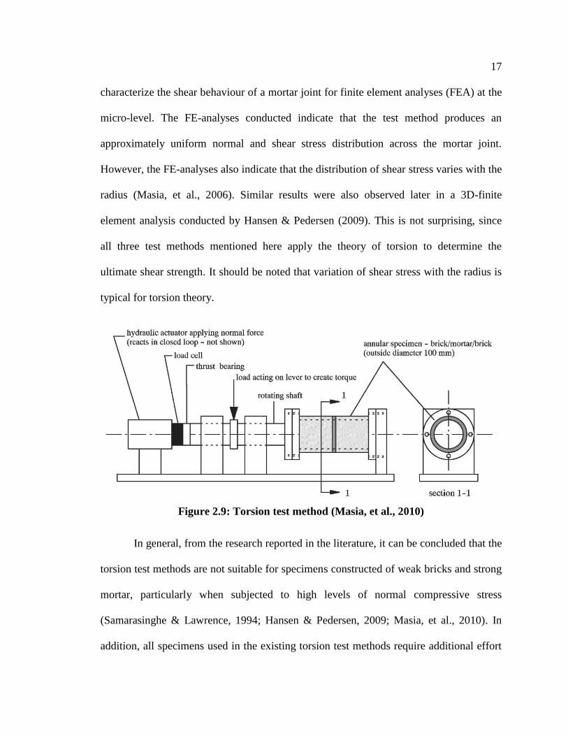
In 2006, Masia et al. proposed a new testing procedure based on the same
principle as used by other researchers for describing the shear strength of a soil specimen,
(Masia, et al., 2006). In the test arrangement shown in Figure 2.9, a specimen consisting
of two annular bricks connected by a mortar joint is subjected to combined normal and
torsion loads. The unique shaped specimen is glued, by means of epoxy, between two
plates in which one plate is fully fixed and the other one is used to induce the loads. Such
a load and support arrangement was also utilized by Khalaf, as discussed above. The
authors reported that the preparation of the specimen with the annular section is the most
time-consuming and challenging part of the test setup (Masia, et al., 2010). In their tests,
the authors attempted to obtain additional information beyond bond shear strength, ,
and coefficient of friction, , such as shear stiffness, shear fracture energy, post cracking
coefficient of friction, and the dilatancy. These additional properties are required to
F
Front view
Top view
FF
17
characterize the shear behaviour of a mortar joint for finite element analyses (FEA) at the
micro-level. The FE-analyses conducted indicate that the test method produces an
approximately uniform normal and shear stress distribution across the mortar joint.
However, the FE-analyses also indicate that the distribution of shear stress varies with the
radius (Masia, et al., 2006). Similar results were also observed later in a 3D-finite
element analysis conducted by Hansen & Pedersen (2009). This is not surprising, since
all three test methods mentioned here apply the theory of torsion to determine the
ultimate shear strength. It should be noted that variation of shear stress with the radius is
typical for torsion theory.
Figure 2.9: Torsion test method (Masia, et al., 2010)
In general, from the research reported in the literature, it can be concluded that the
torsion test methods are not suitable for specimens constructed of weak bricks and strong
mortar, particularly when subjected to high levels of normal compressive stress
(Samarasinghe & Lawrence, 1994; Hansen & Pedersen, 2009; Masia, et al., 2010). In
addition, all specimens used in the existing torsion test methods require additional effort
18
for their preparation, except the one used by Hansen & Pedersen (2009). Further, in the
case of specimens constructed with perforated bricks, the torsion tests are incapable of
producing reasonable results. Beyond that, the torsion tests might be helpful to predict the
torsional shear capacity of a bed joint. However, the torsional shear capacity is only
needed when a stretcher bonded masonry wall is subjected to flexure about an axis
normal to the bed joints which is seldom the case in reality.
2.3 Factors affecting masonry shear strength
The shear strength of a masonry wall as well as of a mortar bed joint is affected
by many different factors. For example, the properties of the unit (such as compressive
strength, anisotropy, size and aspect ratio, absorption properties, condition of the units
during the laying), mortar, and grout as well as the properties of the unit/mortar bond, and
workmanship, (Sutcliffe, et al., 2001). In addition, the shear strength of a mortar bed joint
obtained from a shear test is affected by the presence of normal compressive stress as
well as by the arrangement of the shearing force.
2.3.1 The effect of compressive stress
In 1979, Hamid et al. conducted a research program with 46 specimens
constructed from one type of concrete block and two mortar types (Type S and N), in
which some of the specimens were grouted and some of them not. They observed that
pre-applied normal compressive stress has a significant effect on the results obtained
from a shear test (Hamid, et al., 1979). Similar observations were also made by other
researchers (Pook, et al., 1986; Hofmann & Stöckl, 1986; Hansen, et al., 1998), when
they subjected specimens to combined shear and normal loads using the triplet, and
19
Hofmann & Stöckl tests, respectively. The above mentioned investigations, as well as the
one conducted by Ghazali & Riddington (1986), conclude that the shear strength of a
mortar joint increases linearly with the level of normal compressive stress. This linear
relationship, however, exists only up to a normal compressive stress of about ,
(Riddington & Ghazali, 1987). A normal compressive stress higher than starts
to reduce the rate of increase in shear strength, (Hamid & Drysdale, 1982; Riddington &
Ghazali, 1990). Therefore, in general, it is accepted that the ultimate shear strength, , of
a mortar bed joint subjected to normal compressive stress ( ), follows a
Coulomb relationship (Hamid, et al., 1979; Ghazali & Riddington, 1986; Riddington, et
al., 1997):
(1)
where is the initial bond shear strength or the shear strength at zero normal
compressive stress, and is the coefficient of internal friction at the interface between the
mortar and the unit.
2.3.2 The effect of brick and mortar properties
The effect of brick and mortar properties on the shear behaviour of a mortar bed
joint is controversial in the literature. In 1979, Hamid et al. concluded that shear strength
of a mortar joint is a function of mortar properties as well as of the physical properties of
the block such as surface roughness and initial rate of absorption (Hamid, et al., 1979). A
similar conclusion was reported by Hofmann & Stöckl in 1986. They observed an
increase in ultimate shear stress due to increased compressive strength of clay brick and
20
mortar strength. The increase due to the clay brick strength was related to surface
roughness, condition at laying (i.e. wet or dry), and the corresponding suction capacity of
the bricks (Hofmann & Stöckl, 1986). However, in 1997, Khalaf concluded that an
increase in mortar strength has an effect to a certain extent on the bond shear strength,
and that the type of brick has no significant effect on the bond shear strength (Khalaf &
Naysmith, 1997). The limited effect of an increase in mortar strength was also observed
by Hansen, et al. (1998). In contrast, Vermeltfoort observed an increase in initial shear
strength while the mortar compressive strength was decreased. Therefore, additional
research is suggested to examine the effect of mortar compressive strength on shear
strength (Vermeltfoort, 2010).
2.3.3 The effect of unit aspect ratio and load arrangement
The effect of unit aspect ratio and load arrangement was demonstrated by
researchers who modelled the triplet test with specimens having various unit aspect
ratios, and were subjected to different load and support arrangements. It was concluded
from the analyses that both high and low unit aspect ratios affect the stress distribution
along the mortar joint, and thereby the results of shear strength obtained using the triplet
test. A high unit aspect ratio leads to increased bending in the specimen and a low aspect
ratio leads to concentration of shear stress in the end of the specimen. Further, it was
observed that the load arrangement can lead either to increased or decreased bending in
the specimen depending on the eccentricity of the applied load, (Riddington, et al., 1991;
Bouzeghoub, et al., 1995). The results of a numerical evaluation carried out by the author
for the proposed test method are presented in Chapter 3. The effect of unit aspect ratio
21
was also studied in this case and the results indicate that the stress distribution varies with
the unit aspect ratio. Therefore, it can be concluded that the effect is not specific to any
test method.
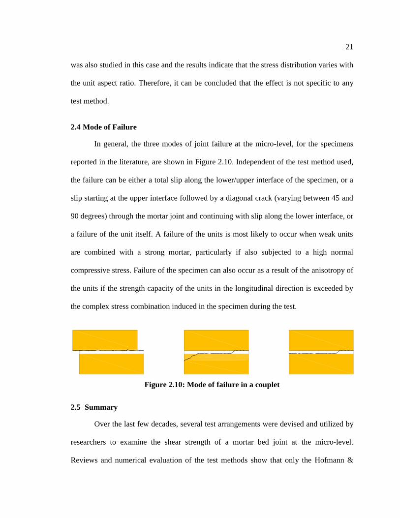
2.4 Mode of Failure
In general, the three modes of joint failure at the micro-level, for the specimens
reported in the literature, are shown in Figure 2.10. Independent of the test method used,
the failure can be either a total slip along the lower/upper interface of the specimen, or a
slip starting at the upper interface followed by a diagonal crack (varying between 45 and
90 degrees) through the mortar joint and continuing with slip along the lower interface, or
a failure of the unit itself. A failure of the units is most likely to occur when weak units
are combined with a strong mortar, particularly if also subjected to a high normal
compressive stress. Failure of the specimen can also occur as a result of the anisotropy of
the units if the strength capacity of the units in the longitudinal direction is exceeded by
the complex stress combination induced in the specimen during the test.
Figure 2.10: Mode of failure in a couplet
2.5 Summary
Over the last few decades, several test arrangements were devised and utilized by
researchers to examine the shear strength of a mortar bed joint at the micro-level.
Reviews and numerical evaluation of the test methods show that only the Hofmann &
22
Stöckl and triplet tests produce reasonable results in term of meeting the criteria as
specified in Chapter 1. The Hofmann & Stöckl test produces the most uniformly
distributed normal and shear stresses along the bed joint, but because it requires very
complex equipment, it is unlikely that the test will be accepted as a standard test method.
Thus, the triplet test is more suitable as a standard test and is more commonly used
although the resulting stress distributions are not ideal. While the Hofmann & Stöckl test
produces the best results and the triplet test is simpler to perform, the challenge remains
to devise a test method that is able to combine the advantages of both test methods. A
new test method has therefore been devised which aims to combine the advantages of the
Hofmann & Stöckl and the triplet test. In the next chapter, the new test method is
analyzed using finite element analyses.
23
CHAPTER 3: NUMERICAL EVALUATION
3.1 Introduction
The results of numerical analyses of mortar joint shear tests reported in the
literature in the last 20 years indicates that the Hofmann & Stöckl and triplet test are most
capable of producing the most desirable results with respect to criteria specified by
Riddington et al. (1997). The main purpose of the numerical evaluations described in this
chapter is to gain insight into the state of stress distribution imposed in the mortar joint by
the proposed test method, and to compare the distribution with the stress distributions
imposed by the two existing joint shear test methods (triplet and Hofmann & Stöckl
tests). Therefore, the results of numerical analyses of the two existing test methods in
addition to the one proposed in this chapter are discussed.
3.2 Material Properties
The brick chosen for the analyses of each test method are assumed to be solid clay
brick with typical dimensions used in North America ( ):
(Model 1), and those used in an earlier study by Hofmann & Stöckl (1986):
(Model 2). This step enables the comparison between the results of
the original Hofmann & Stöckl test and the proposed one, and it also indicates to what
extent the brick dimensions affect the test results.
The basic properties of the brick as well as of the mortar, assumed for the FEM
analyses, are based on the existing literature, and are summarized in Table 3.1.
24
Table 3.1: Assumed Material Properties
Material Modulus of Elasticity
(N/mm2)
Poison’s ratio,
Brick 25500 0.13
Mortar 8500 0.18
Steel 200000 0.30
3.3 Modelling Strategy
A two-dimensional finite element model of the test methods based on linear
stress-strain behaviour of material was deemed to be sufficient to gain insight into the
state of stress distribution imposed in the mortar bed joints. The non-linearity of the
mortar does not affect the mode of initial failure or the corresponding load, and only
affects the stress distribution along the joint at a high level of pre-compression,
(Bouzeghoub, et al., 1995).
For the numerical evaluation, two case studies (Case Study 1 and 2) were
conducted using the commercial software package SAP2000 version 14. In Case Study 1,
the numerical results reported in the literature were first reproduced by using the same
elements, loads and boundary conditions as used in the original numerical evaluations.
This step allows comparison of the results obtained for the proposed test method with the
numerical results reported in the literature for the two existing tests, and validates the
results obtained in the current analyses, especially the results of the proposed test method.
In Case Study 2, a few modifications were made to account for the actual boundary
conditions in the tests as explained in Section 3.3.2. Furthermore, a mesh sensitivity
analysis was carried out by examining the results using various mesh sizes. The use of 8
node elements was also considered for Case Study 2, however convergence for mesh
25
sizes 10, 5, and 2.5 mm was not possible due to mesh size limitations in the software for
8 node elements. Therefore, elements with 4 nodes but half of the size (5, 2.5, and 1.25
mm) of the elements with 8 nodes were used. Table 3.2 shows that the 4 node elements
utilized produce results with a difference less than 3% when comparing the X, Y, Z
deformations (U1, U2, U3) at an arbitrarily chosen node.
Table 3.2: Mesh refinement
8 Node elements 4 Node elements Difference
10 mm 5 mm 5 mm 2.5 mm
U1 0.116 0.0804 0.113 0.0791 2.5% 1.6%
U2 0 0 0 0 0% 0%
U3 -0.0114 -0.0094 -0.0114 -0.0092 0% 2.1%
In Figure 3.1, the results for the displacement obtained using 4 node elements
with different mesh sizes (10, 5, 2.5, and 1.25 mm) are plotted versus the number of mesh
elements, from left to right respectively. It can be seen that convergence starts at a mesh
size of 5 mm. Therefore, it was concluded that a mesh size of 5 mm or lower provides
results that are accurate enough for the purpose of this study.
26
Figure 3.1: Mesh convergence
Hence, for the numerical analyses of the joint shear tests, elements with 4 nodes
and isotropic behaviour are used for the brick, mortar, and steel by assuming plane stress.
In both case studies, the applied horizontal loads should cause, depending on the bed joint
area of each specimen, an average shear stress with a magnitude of ⁄ along
the mortar joint. No external load, normal to the bed joint, is applied to the specimens,
except in the Hofmann & Stöckl test, since this test can be performed only in the
presence of pre-compression.
3.3.1 Case Study 1
In the following, the finite element models for the triplet, Hofmann & Stöckl, and
the proposed test method are described, analyzed, and the corresponding results are
discussed.
10 mm
5 mm
2.5 mm
1.25 mm
0
0.02
0.04
0.06
0.08
0.1
0.12
0.14
0.16
0.18
0 5000 10000 15000 20000 25000 30000 35000
Dis
pla
cem
ent,
mm
Number of elements
27
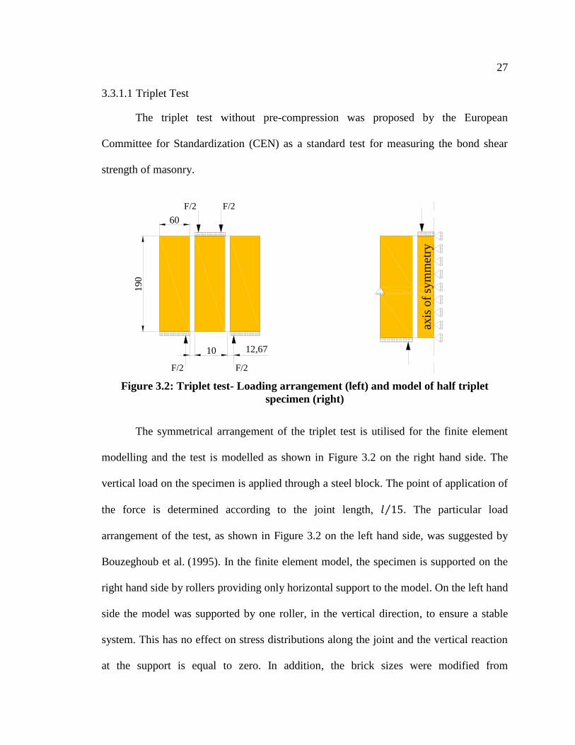
3.3.1.1 Triplet Test
The triplet test without pre-compression was proposed by the European
Committee for Standardization (CEN) as a standard test for measuring the bond shear
strength of masonry.
Figure 3.2: Triplet test- Loading arrangement (left) and model of half triplet
specimen (right)
The symmetrical arrangement of the triplet test is utilised for the finite element
modelling and the test is modelled as shown in Figure 3.2 on the right hand side. The
vertical load on the specimen is applied through a steel block. The point of application of
the force is determined according to the joint length, ⁄ . The particular load
arrangement of the test, as shown in Figure 3.2 on the left hand side, was suggested by
Bouzeghoub et al. (1995). In the finite element model, the specimen is supported on the
right hand side by rollers providing only horizontal support to the model. On the left hand
side the model was supported by one roller, in the vertical direction, to ensure a stable
system. This has no effect on stress distributions along the joint and the vertical reaction
at the support is equal to zero. In addition, the brick sizes were modified from
190
12,67
60
10
F/2
F/2
F/2
F/2
axis
of
sym
met
ry
28
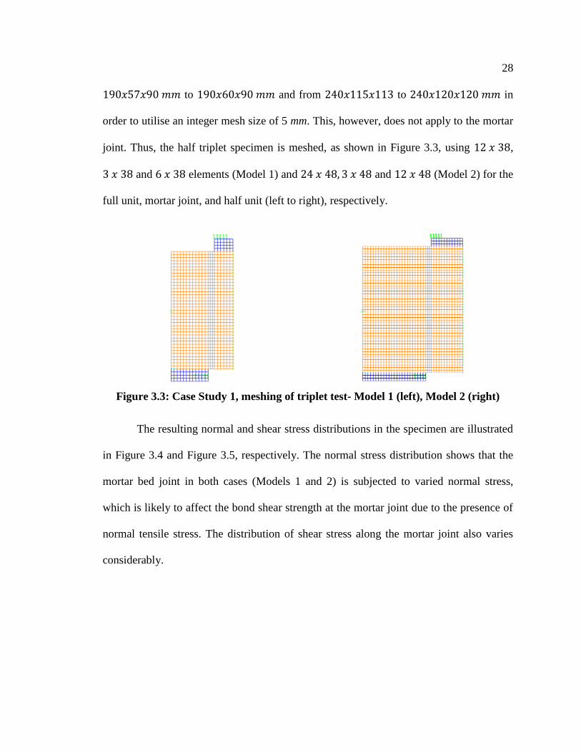
to and from to in
order to utilise an integer mesh size of 5 mm. This, however, does not apply to the mortar
joint. Thus, the half triplet specimen is meshed, as shown in Figure 3.3, using ,
and elements (Model 1) and and (Model 2) for the
full unit, mortar joint, and half unit (left to right), respectively.
Figure 3.3: Case Study 1, meshing of triplet test- Model 1 (left), Model 2 (right)
The resulting normal and shear stress distributions in the specimen are illustrated
in Figure 3.4 and Figure 3.5, respectively. The normal stress distribution shows that the
mortar bed joint in both cases (Models 1 and 2) is subjected to varied normal stress,
which is likely to affect the bond shear strength at the mortar joint due to the presence of
normal tensile stress. The distribution of shear stress along the mortar joint also varies
considerably.
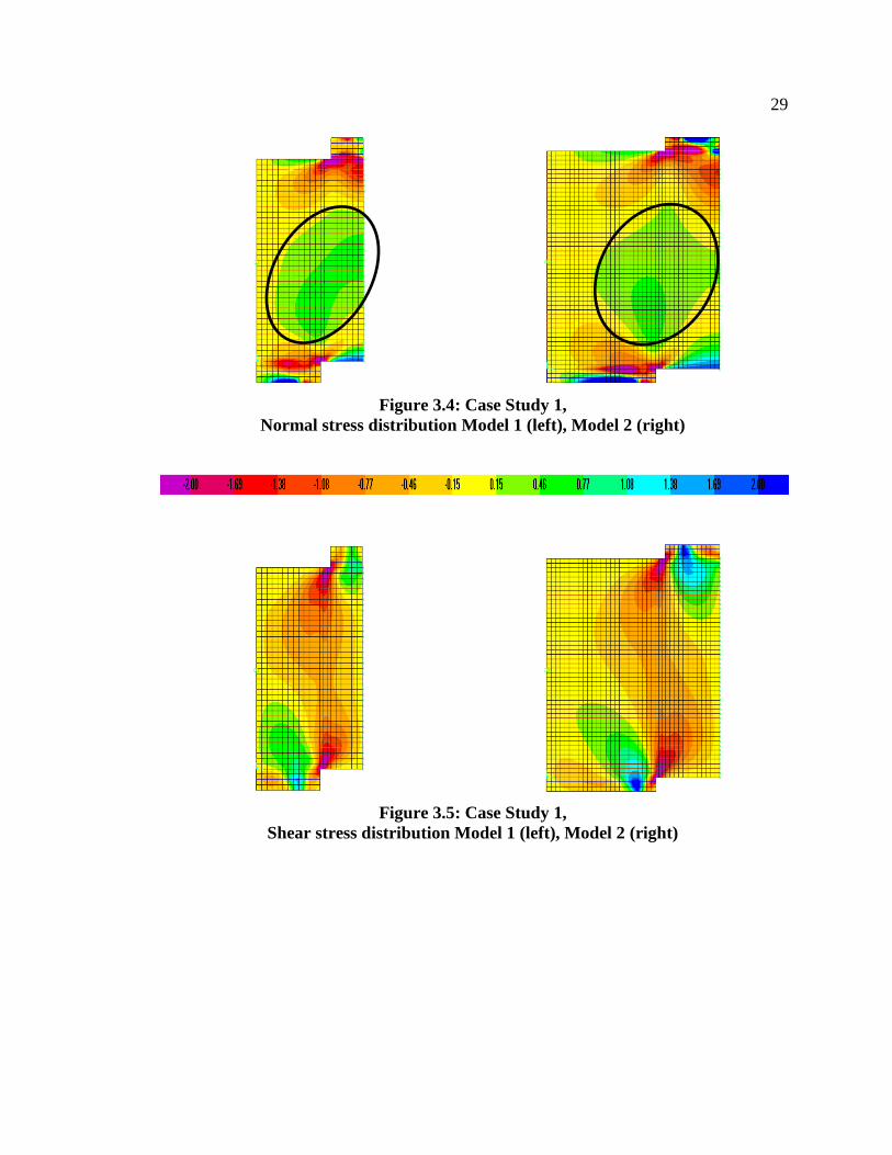
29
Figure 3.4: Case Study 1,
Normal stress distribution Model 1 (left), Model 2 (right)
Figure 3.5: Case Study 1,
Shear stress distribution Model 1 (left), Model 2 (right)
30
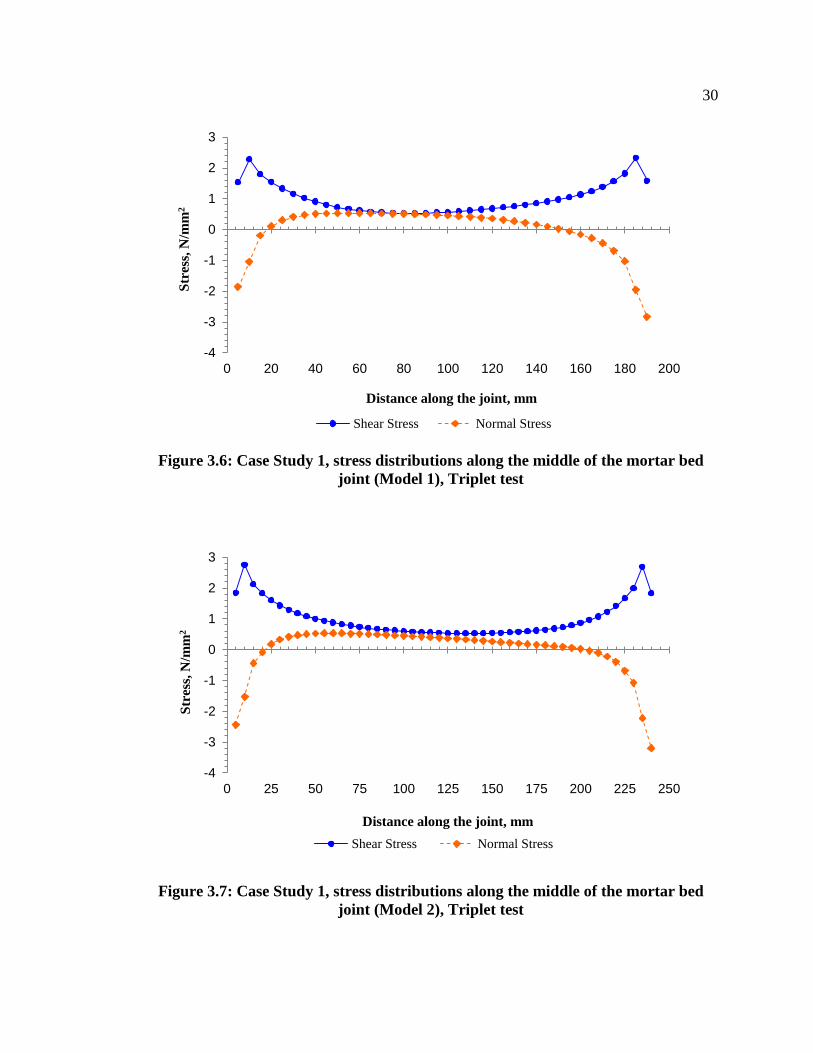
Figure 3.6: Case Study 1, stress distributions along the middle of the mortar bed
joint (Model 1), Triplet test
Figure 3.7: Case Study 1, stress distributions along the middle of the mortar bed
joint (Model 2), Triplet test
-4
-3
-2
-1
0
1
2
3
0 20 40 60 80 100 120 140 160 180 200
Str
ess,
N/m
m2
Distance along the joint, mm
Shear Stress Normal Stress
-4
-3
-2
-1
0
1
2
3
0 25 50 75 100 125 150 175 200 225 250
Str
ess,
N/m
m2
Distance along the joint, mm
Shear Stress Normal Stress
31
The magnitude of the normal and shear stresses along the length at the mid-height
of the joint are illustrated in Figure 3.6 and Figure 3.7. The shear stress deviates from the
average imposed shear stress of by more than at the ends and up
to at the mid-length of the joint. This state of shear stress combined with the
likewise varied normal stress leads to uncertainty whether the failure of the specimen is a
result of the shear stress or of normal tensile stress, and whether the obtained results for
bond shear strength represent the actual bond shear strength of the mortar joint or not.
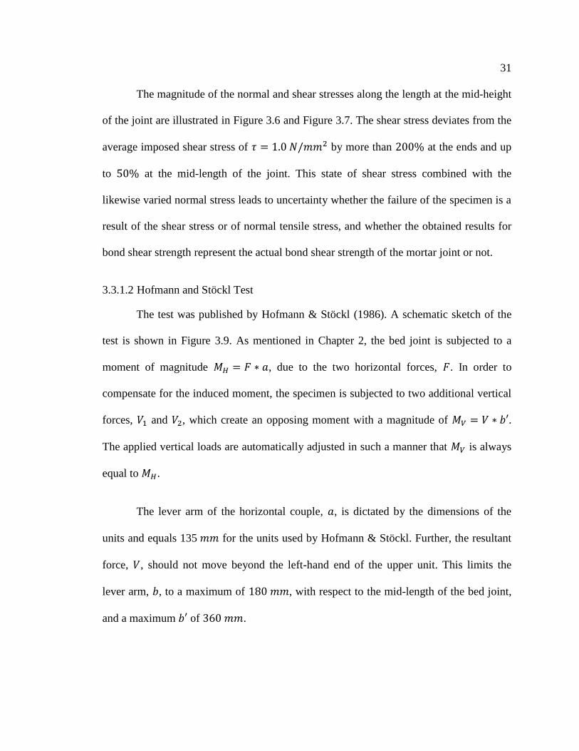
3.3.1.2 Hofmann and Stöckl Test
The test was published by Hofmann & Stöckl (1986). A schematic sketch of the
test is shown in Figure 3.9. As mentioned in Chapter 2, the bed joint is subjected to a
moment of magnitude , due to the two horizontal forces, . In order to
compensate for the induced moment, the specimen is subjected to two additional vertical
forces, and , which create an opposing moment with a magnitude of .
The applied vertical loads are automatically adjusted in such a manner that is always
equal to .
The lever arm of the horizontal couple, , is dictated by the dimensions of the
units and equals 135 for the units used by Hofmann & Stöckl. Further, the resultant
force, , should not move beyond the left-hand end of the upper unit. This limits the
lever arm, , to a maximum of , with respect to the mid-length of the bed joint,
and a maximum of .
32
Figure 3.8: Hofmann and Stöckl Test
In Case Study 1, the finite element analyses for Models 1 and 2 are conducted in
nearly the same manner as was done originally by Stöckl & Hofmann (1990), as shown in
Figure 3.9, except that the factor for the vertical linear load (P2’) is modified and
adjusted. It was determined that the factor presented by Stöckl & Hofmann (1990) for the
vertical linear load (P2’) caused a moment greater than that imposed by the horizontal
load (P) and leads to overturning of the specimen. Therefore, in the case of Model 2, the
factor (P2’) is modified as shown in Eq. (2) and in case of Model 1, the factor is adjusted
to the different unit and joint sizes, as shown in Eq. (3).
( )
( )
(2)
( )
( )
(3)
V1 V2
F
V
V
b'
F
a
V1 V2
440
50 230 110 50
F
F
135
V
b
33
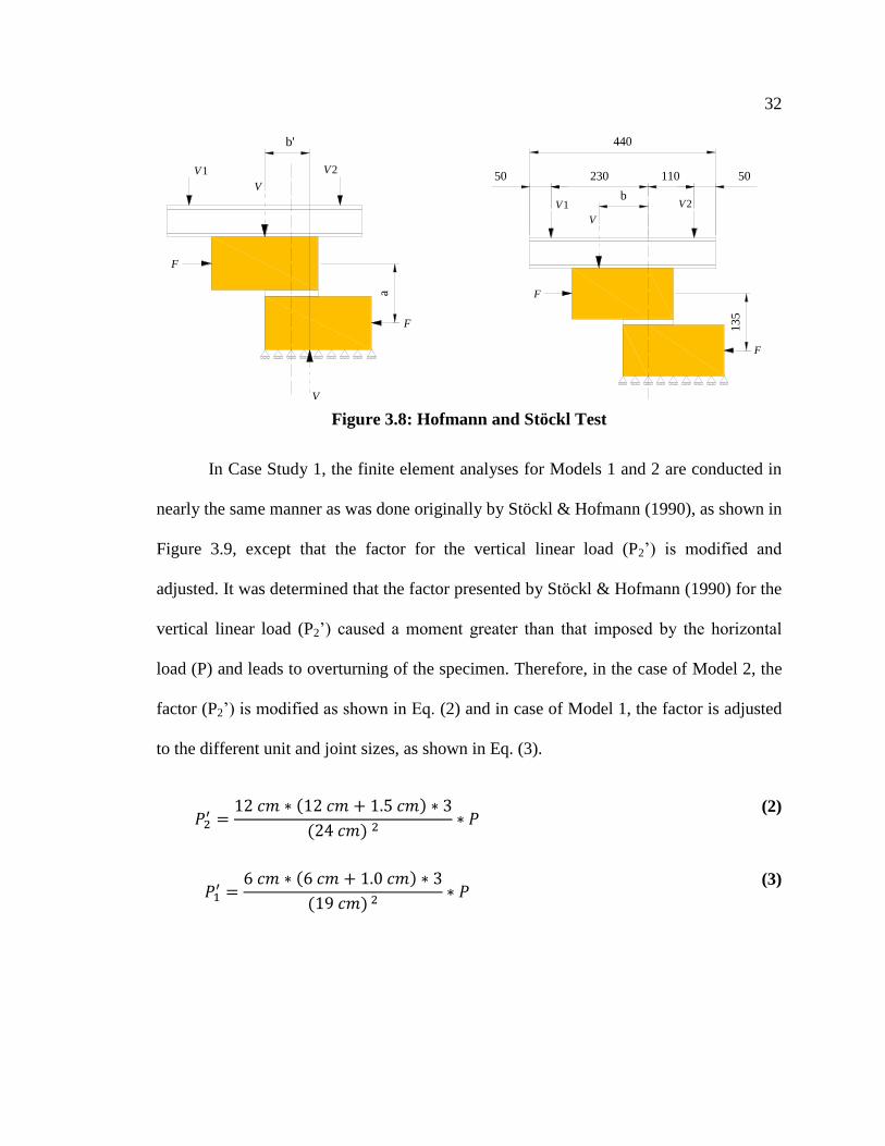
Figure 3.9: Hofmann and Stöckl Test - Model 1 (left), Model 2 (right)
Figure 3.10 presents the finite element models used for the analyses. In the two
models shown, all nodes in the bottom are supported by rollers in the vertical direction,
except the last one on the right hand side. This one is declared as a pin to ensure a stable
system. Its reaction in the horizontal direction is equal to zero and has no effect on the
stress distribution. The couplet itself is subjected to horizontal load as well as to vertical
load. Both the vertical and horizontal loads are applied through a steel block. Except for
the mortar joint in Model 1, square elements with a size of were used to mesh
Models 1 and 2. For the mortar joint in Model 1 rectangular elements with a size of
( ) were used. Thus, the units and joints are divided into ,
and elements (Model 1) and , and elements
(Model 2), for the lower brick, joint, and upper brick, respectively.
P
P
P1'
P1'
190
60
10
95
P
P
P2'
P2'
240
15
120 120
P2’ P2’
P1’
P1’
34
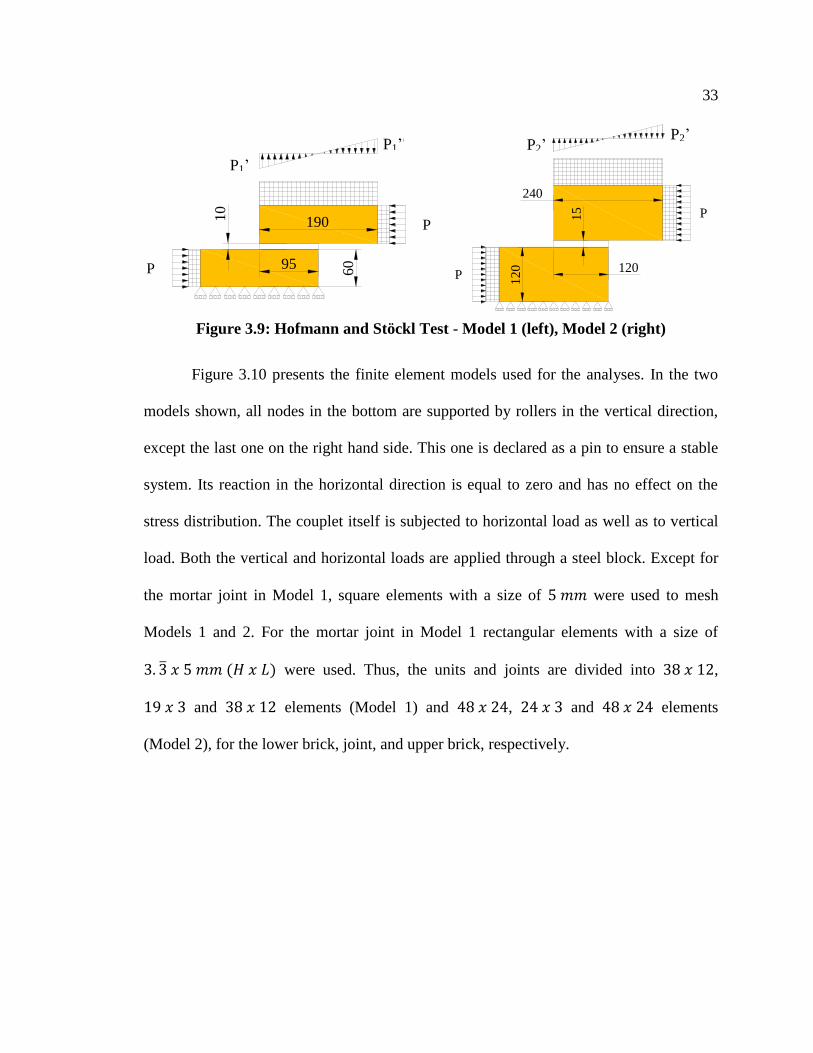
Figure 3.10: Case Study 1, FE models of Hofmann and Stöckl test- Model 1 (left),
Model 2 (right)
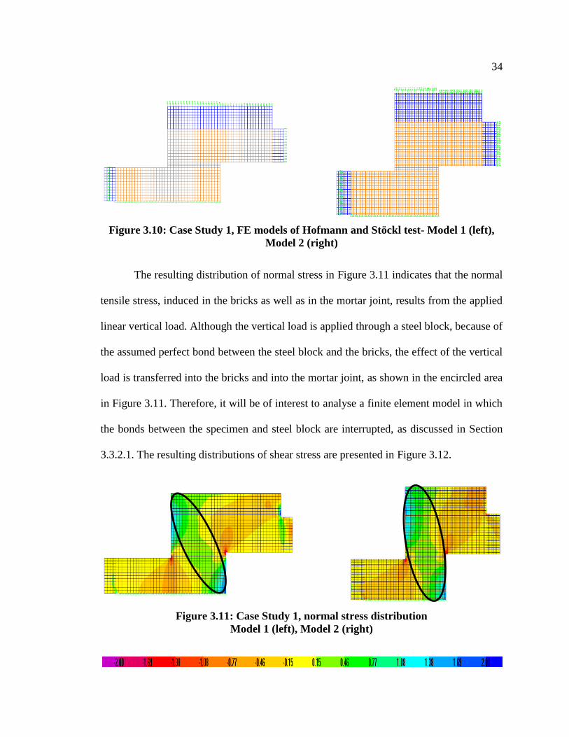
The resulting distribution of normal stress in Figure 3.11 indicates that the normal
tensile stress, induced in the bricks as well as in the mortar joint, results from the applied
linear vertical load. Although the vertical load is applied through a steel block, because of
the assumed perfect bond between the steel block and the bricks, the effect of the vertical
load is transferred into the bricks and into the mortar joint, as shown in the encircled area
in Figure 3.11. Therefore, it will be of interest to analyse a finite element model in which
the bonds between the specimen and steel block are interrupted, as discussed in Section
3.3.2.1. The resulting distributions of shear stress are presented in Figure 3.12.
Figure 3.11: Case Study 1, normal stress distribution
Model 1 (left), Model 2 (right)
35
Figure 3.12: Case Study 1, shear stress distribution
Model 1 (left), Model 2 (right)
In Figure 3.13 and Figure 3.14, the magnitude of normal and shear stress at mid-
height of the joint are illustrated along the length of the mortar bed joint in . As
expected, the distributions of the shear and normal stresses in the Hofmann and Stöckl
test are more uniform than in the triplet test. The different distributions of normal and
shear stress in Models 1 and 2 indicate that the results of Hofmann & Stöckl test are
affected by the unit size.
The results of Model 2 determined in the current analysis by using the modified
factor for the vertical load, P2’, are identical to those obtained originally (Stöckl &
Hofmann, 1990; Riddington, et al., 1997).
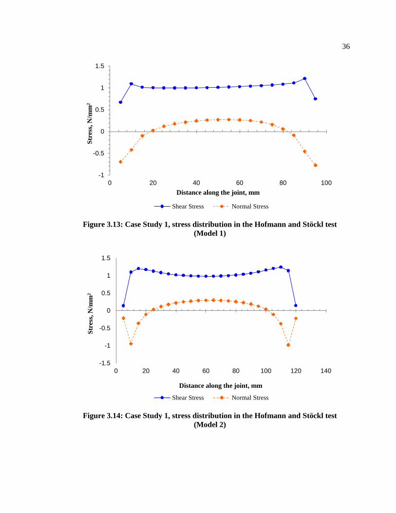
36
Figure 3.13: Case Study 1, stress distribution in the Hofmann and Stöckl test
(Model 1)
Figure 3.14: Case Study 1, stress distribution in the Hofmann and Stöckl test
(Model 2)
-1
-0.5
0
0.5
1
1.5
0 20 40 60 80 100
Str
ess,
N/m
m2
Distance along the joint, mm
Shear Stress Normal Stress
-1.5
-1
-0.5
0
0.5
1
1.5
0 20 40 60 80 100 120 140
Str
ess,
N/m
m2
Distance along the joint, mm
Shear Stress Normal Stress
37
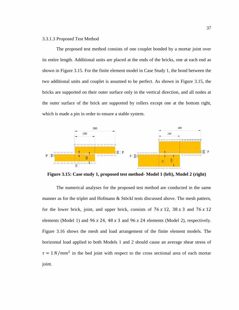
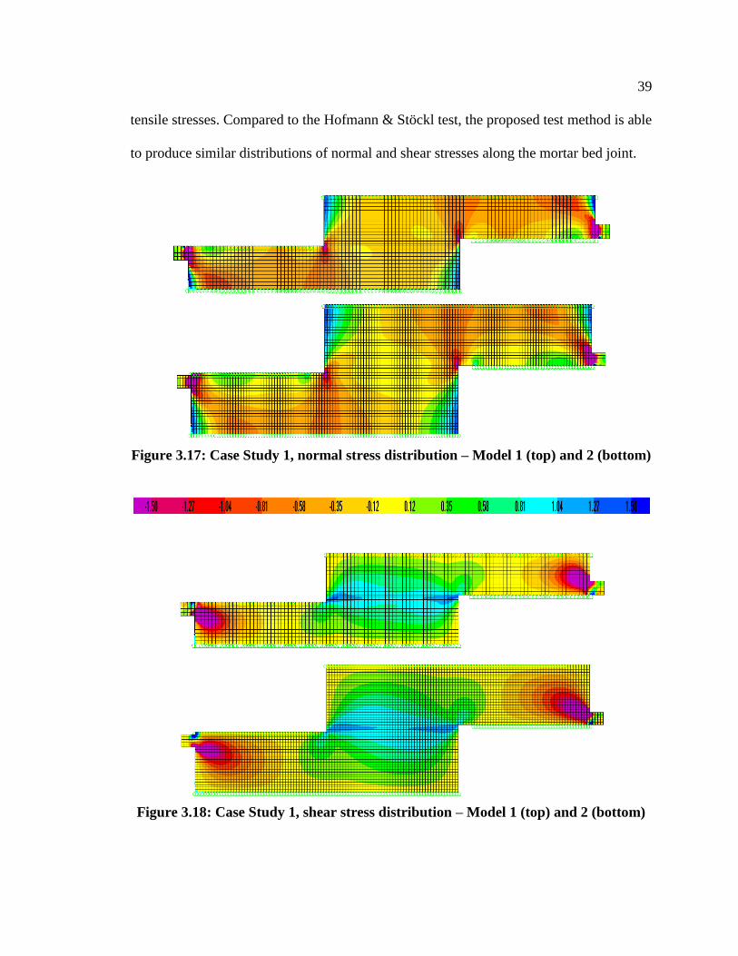
3.3.1.3 Proposed Test Method
The proposed test method consists of one couplet bonded by a mortar joint over
its entire length. Additional units are placed at the ends of the bricks, one at each end as
shown in Figure 3.15. For the finite element model in Case Study 1, the bond between the
two additional units and couplet is assumed to be perfect. As shown in Figure 3.15, the
bricks are supported on their outer surface only in the vertical direction, and all nodes at
the outer surface of the brick are supported by rollers except one at the bottom right,
which is made a pin in order to ensure a stable system.
Figure 3.15: Case study 1, proposed test method- Model 1 (left), Model 2 (right)
The numerical analyses for the proposed test method are conducted in the same
manner as for the triplet and Hofmann & Stöckl tests discussed above. The mesh pattern,
for the lower brick, joint, and upper brick, consists of , and
elements (Model 1) and , and elements (Model 2), respectively.
Figure 3.16 shows the mesh and load arrangement of the finite element models. The
horizontal load applied to both Models 1 and 2 should cause an average shear stress of
⁄ in the bed joint with respect to the cross sectional area of each mortar
joint.
60
10
380
P
190
P
120
15
P
P
480
240
38
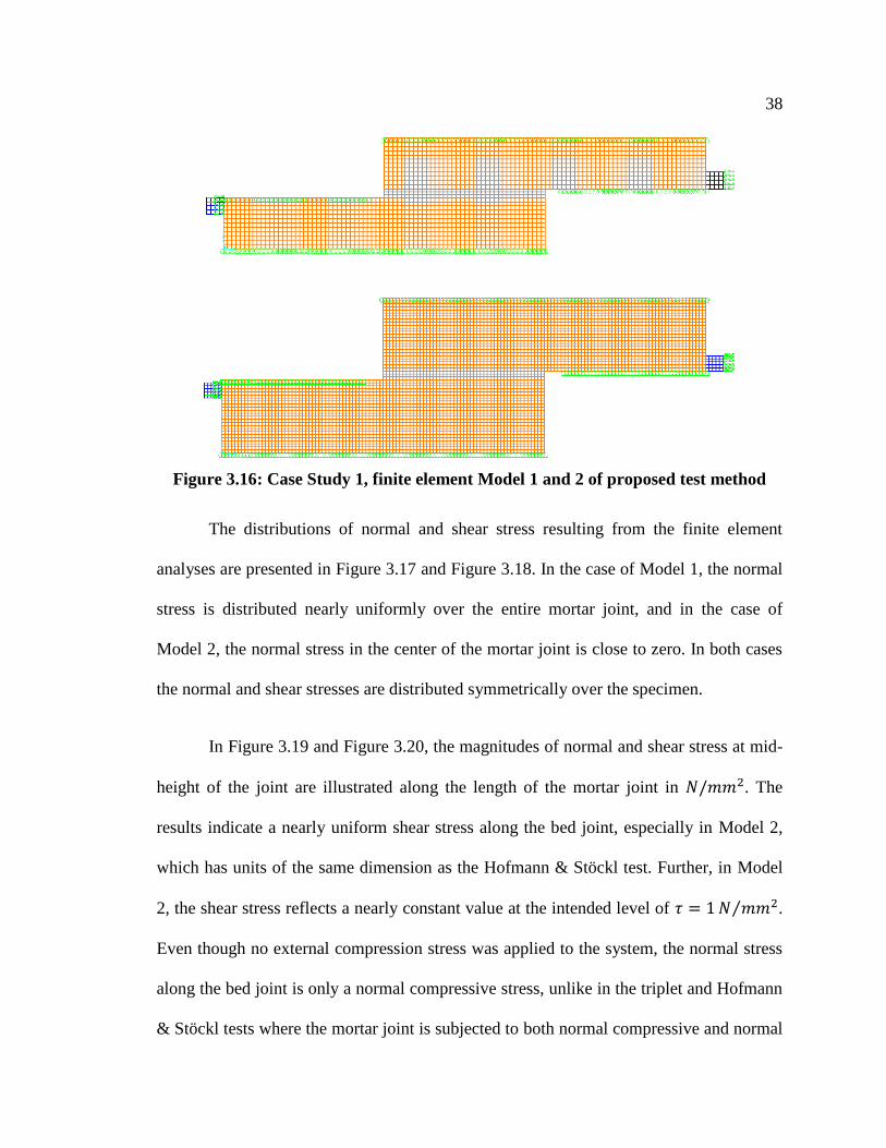
Figure 3.16: Case Study 1, finite element Model 1 and 2 of proposed test method
The distributions of normal and shear stress resulting from the finite element
analyses are presented in Figure 3.17 and Figure 3.18. In the case of Model 1, the normal
stress is distributed nearly uniformly over the entire mortar joint, and in the case of
Model 2, the normal stress in the center of the mortar joint is close to zero. In both cases
the normal and shear stresses are distributed symmetrically over the specimen.
In Figure 3.19 and Figure 3.20, the magnitudes of normal and shear stress at mid-
height of the joint are illustrated along the length of the mortar joint in . The
results indicate a nearly uniform shear stress along the bed joint, especially in Model 2,
which has units of the same dimension as the Hofmann & Stöckl test. Further, in Model
2, the shear stress reflects a nearly constant value at the intended level of ⁄ .
Even though no external compression stress was applied to the system, the normal stress
along the bed joint is only a normal compressive stress, unlike in the triplet and Hofmann
& Stöckl tests where the mortar joint is subjected to both normal compressive and normal
39
tensile stresses. Compared to the Hofmann & Stöckl test, the proposed test method is able
to produce similar distributions of normal and shear stresses along the mortar bed joint.
Figure 3.17: Case Study 1, normal stress distribution – Model 1 (top) and 2 (bottom)
Figure 3.18: Case Study 1, shear stress distribution – Model 1 (top) and 2 (bottom)
40
Figure 3.19: Case Study 1, stress distribution in the proposed test method
(Model 1)
Figure 3.20: Case Study 1, stress distribution in the proposed test method
(Model 2)
-1.5
-1
-0.5
0
0.5
1
1.5
0 20 40 60 80 100 120 140 160 180 200
Str
ess,
N/m
m2
Distance along the joint, mm
Shear Stress Normal Stress
-1.5
-1
-0.5
0
0.5
1
1.5
0 25 50 75 100 125 150 175 200 225 250
Str
ess,
N/m
m2
Distance along the joint, mm
Shear Stress Normal Stress
41
The difference between Models 1 and 2 in the distributions of normal and shear
stresses reveals that the results of the proposed test method are affected by the
dimensions of the units. Therefore, three additional analyses using Models 3, 4 and 5
were conducted. In the first additional analysis (Model 3), the dimension of the brick is
modified to ( ), in order to study the effect of aspect ratio
(height/length) of the brick. In the second additional analysis (Model 4), the original
specimen used by Hofmann & Stöckl is subjected to the boundary conditions of the
proposed test method, and in the third additional model (Model 5), the dimensions of the
specimen of Model 4 are modified from to .
The latter two analyses, Models 4 and 5, are carried out to determine the response of the
proposed test method to different shapes of specimen and different slopes of the
theoretical load path between the two points of load application. All three additional
finite element analyses were performed similarly to the previous ones, and the additional
finite element models were meshed, for the lower brick, joint, and upper brick, with
, and elements (Model 3), , and elements
(Model 4) and , and elements (Model 5), respectively. A square
mesh size of was used for the bricks and mortar in case of Model 4, and a
rectangular mesh size of was used in the case of Models 3 and 5.
The analyses using Models 3, 4 and 5, for the proposed test method, were
performed with varied points of load application. From these analyses, it was noticed that
the change in the theoretical slope of the load path between the two points of load
application did not have a significant effect on the distribution of normal and shear
42
stresses. However, the change in the aspect ratio of the brick affects the results, as can be
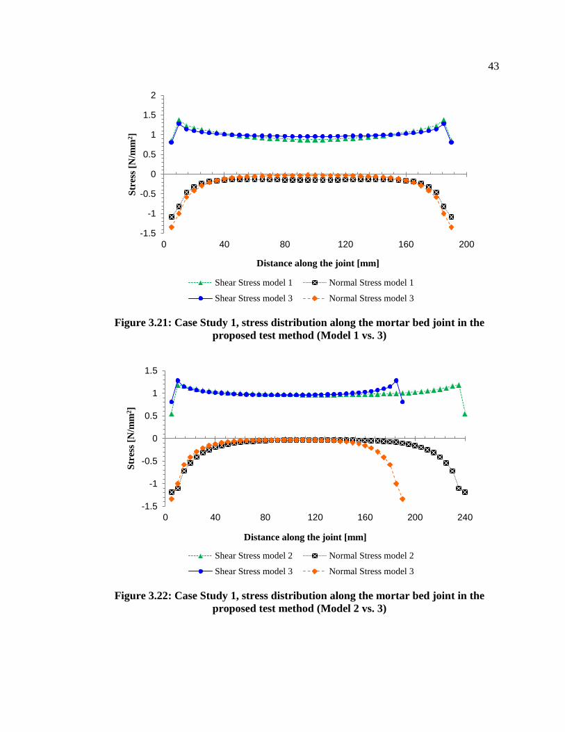
seen by comparing Model 1 and 3 in Figure 3.21. Further, it was noticed that despite the
different length of mortar joint, the results for the proposed test method and a particular
unit aspect ratio are constant. For example, the height to length ratio of the units utilized
in Model 2 ( ) as well as in Model 3 ( ) is equal to . The
distribution of normal and shear stresses in both cases are exactly the same, as seen in
Figure 3.22.
Comparison of the original Hofmann & Stöckl test (Model 2) analyses to the
proposed test method in Model 4 shows that the proposed test method is capable of
producing similar, if not better, results. The distribution of shear stress, as shown in
Figure 3.23, is identical to the one produced in Model 2 of the Hofmann & Stöckl test.
The normal stress along the mortar joint in Model 4 is offset such that the mortar joint is
subjected only to normal compressive stress. However, the distribution is similar to the
one produced in Model 2 of the Hofmann & Stöckl test. Comparison of the results from
the Hofmann & Stöckl test with modified unit size (Model 1), to the results of Model 5,
are shown in Figure 3.24. Again, it is clear that the proposed test method is capable of
producing results at least as good as the Hofmann & Stöckl test.
43
Figure 3.21: Case Study 1, stress distribution along the mortar bed joint in the
proposed test method (Model 1 vs. 3)
Figure 3.22: Case Study 1, stress distribution along the mortar bed joint in the
proposed test method (Model 2 vs. 3)
-1.5
-1
-0.5
0
0.5
1
1.5
2
0 40 80 120 160 200
Str
ess
[N/m
m2]
Distance along the joint [mm]
Shear Stress model 1 Normal Stress model 1
Shear Stress model 3 Normal Stress model 3
-1.5
-1
-0.5
0
0.5
1
1.5
0 40 80 120 160 200 240
Str
ess
[N/m
m2]
Distance along the joint [mm]
Shear Stress model 2 Normal Stress model 2
Shear Stress model 3 Normal Stress model 3
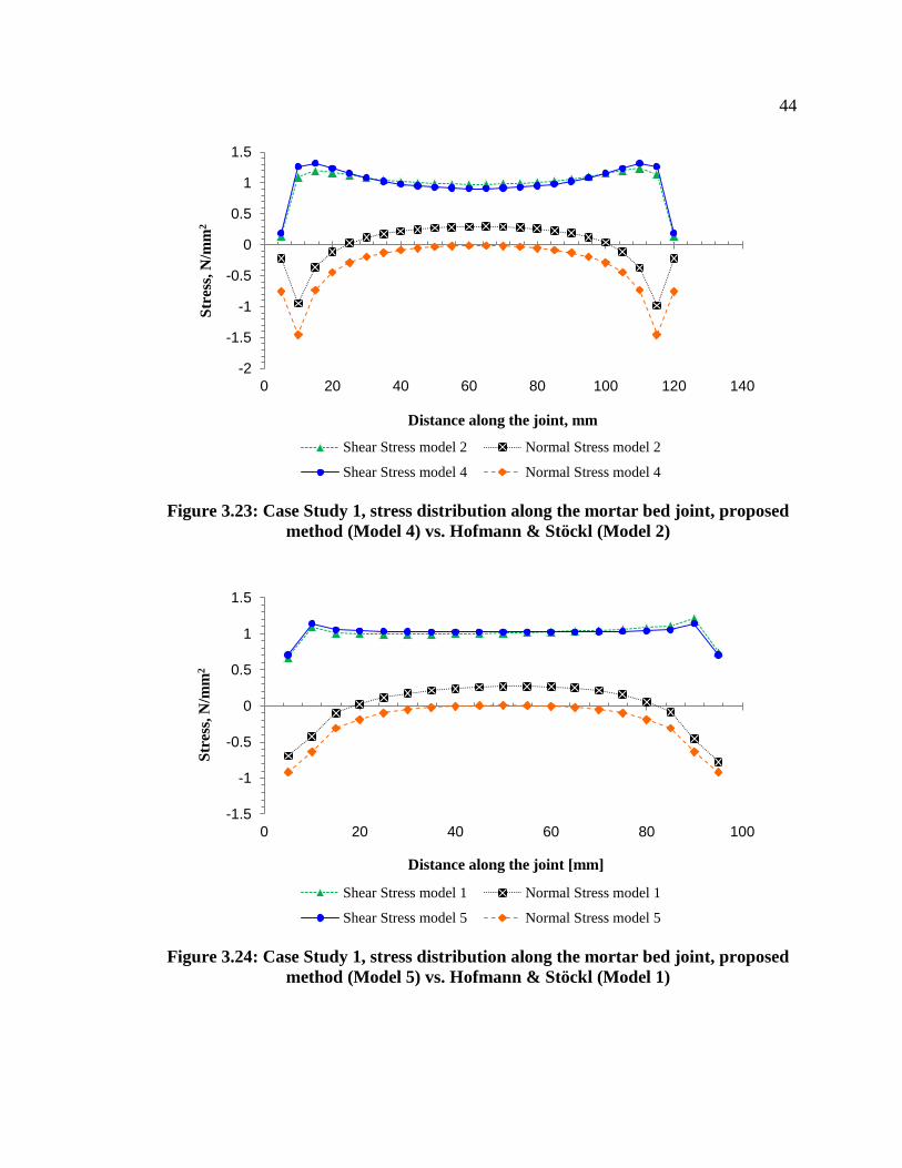
44
Figure 3.23: Case Study 1, stress distribution along the mortar bed joint, proposed
method (Model 4) vs. Hofmann & Stöckl (Model 2)
Figure 3.24: Case Study 1, stress distribution along the mortar bed joint, proposed
method (Model 5) vs. Hofmann & Stöckl (Model 1)
-2
-1.5
-1
-0.5
0
0.5
1
1.5
0 20 40 60 80 100 120 140
Str
ess,
N/m
m2
Distance along the joint, mm
Shear Stress model 2 Normal Stress model 2
Shear Stress model 4 Normal Stress model 4
-1.5
-1
-0.5
0
0.5
1
1.5
0 20 40 60 80 100
Str
ess,
N/m
m2
Distance along the joint [mm]
Shear Stress model 1 Normal Stress model 1
Shear Stress model 5 Normal Stress model 5
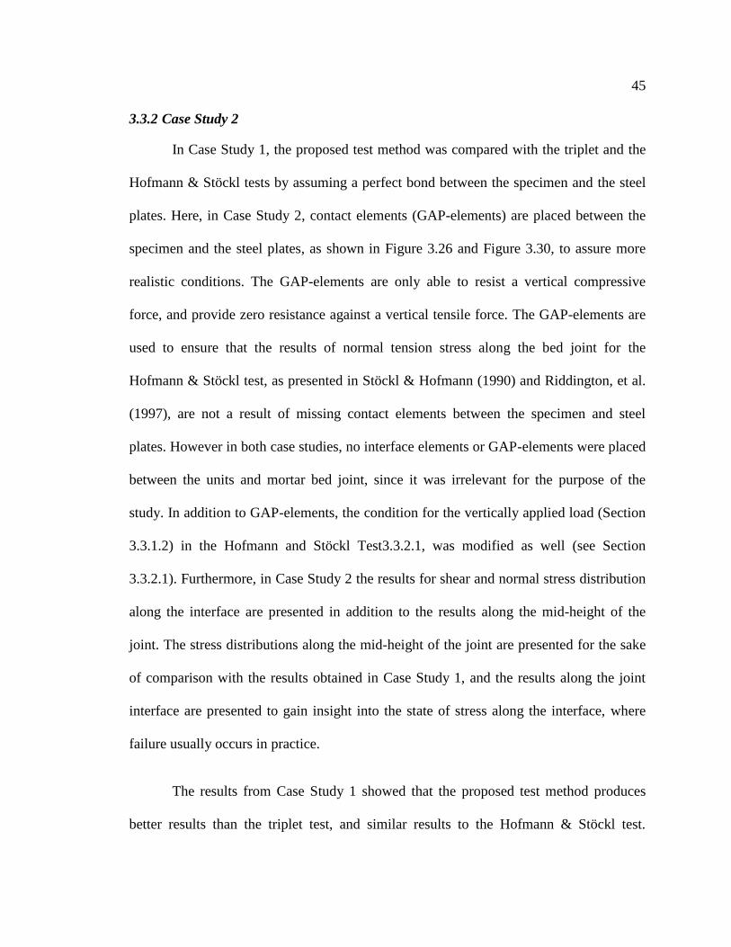
45
3.3.2 Case Study 2
In Case Study 1, the proposed test method was compared with the triplet and the
Hofmann & Stöckl tests by assuming a perfect bond between the specimen and the steel
plates. Here, in Case Study 2, contact elements (GAP-elements) are placed between the
specimen and the steel plates, as shown in Figure 3.26 and Figure 3.30, to assure more
realistic conditions. The GAP-elements are only able to resist a vertical compressive
force, and provide zero resistance against a vertical tensile force. The GAP-elements are
used to ensure that the results of normal tension stress along the bed joint for the
Hofmann & Stöckl test, as presented in Stöckl & Hofmann (1990) and Riddington, et al.
(1997), are not a result of missing contact elements between the specimen and steel
plates. However in both case studies, no interface elements or GAP-elements were placed
between the units and mortar bed joint, since it was irrelevant for the purpose of the
study. In addition to GAP-elements, the condition for the vertically applied load (Section
3.3.1.2) in the Hofmann and Stöckl Test3.3.2.1, was modified as well (see Section
3.3.2.1). Furthermore, in Case Study 2 the results for shear and normal stress distribution
along the interface are presented in addition to the results along the mid-height of the
joint. The stress distributions along the mid-height of the joint are presented for the sake
of comparison with the results obtained in Case Study 1, and the results along the joint
interface are presented to gain insight into the state of stress along the interface, where
failure usually occurs in practice.
The results from Case Study 1 showed that the proposed test method produces
better results than the triplet test, and similar results to the Hofmann & Stöckl test.
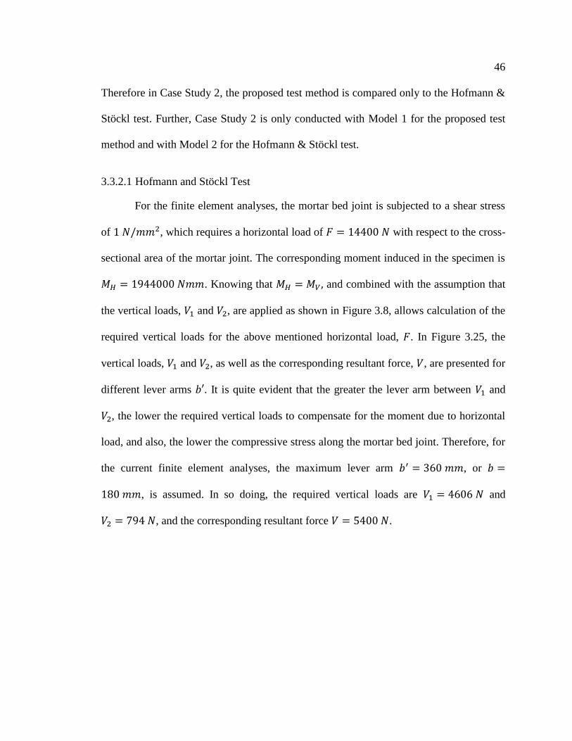
46
Therefore in Case Study 2, the proposed test method is compared only to the Hofmann &
Stöckl test. Further, Case Study 2 is only conducted with Model 1 for the proposed test
method and with Model 2 for the Hofmann & Stöckl test.
3.3.2.1 Hofmann and Stöckl Test
For the finite element analyses, the mortar bed joint is subjected to a shear stress
of , which requires a horizontal load of with respect to the cross-
sectional area of the mortar joint. The corresponding moment induced in the specimen is
. Knowing that and combined with the assumption that
the vertical loads, and , are applied as shown in Figure 3.8, allows calculation of the
required vertical loads for the above mentioned horizontal load, . In Figure 3.25, the
vertical loads, and , as well as the corresponding resultant force, , are presented for
different lever arms . It is quite evident that the greater the lever arm between and
, the lower the required vertical loads to compensate for the moment due to horizontal
load, and also, the lower the compressive stress along the mortar bed joint. Therefore, for
the current finite element analyses, the maximum lever arm , or
, is assumed. In so doing, the required vertical loads are and
, and the corresponding resultant force .
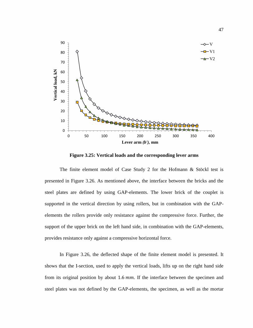
47
Figure 3.25: Vertical loads and the corresponding lever arms
The finite element model of Case Study 2 for the Hofmann & Stöckl test is
presented in Figure 3.26. As mentioned above, the interface between the bricks and the
steel plates are defined by using GAP-elements. The lower brick of the couplet is
supported in the vertical direction by using rollers, but in combination with the GAP-
elements the rollers provide only resistance against the compressive force. Further, the
support of the upper brick on the left hand side, in combination with the GAP-elements,
provides resistance only against a compressive horizontal force.
In Figure 3.26, the deflected shape of the finite element model is presented. It
shows that the I-section, used to apply the vertical loads, lifts up on the right hand side
from its original position by about . If the interface between the specimen and
steel plates was not defined by the GAP-elements, the specimen, as well as the mortar
0
10
20
30
40
50
60
70
80
90
0 50 100 150 200 250 300 350 400
Ver
tica
l lo
ad
, k
N
Lever arm (b'), mm
V
V1
V2
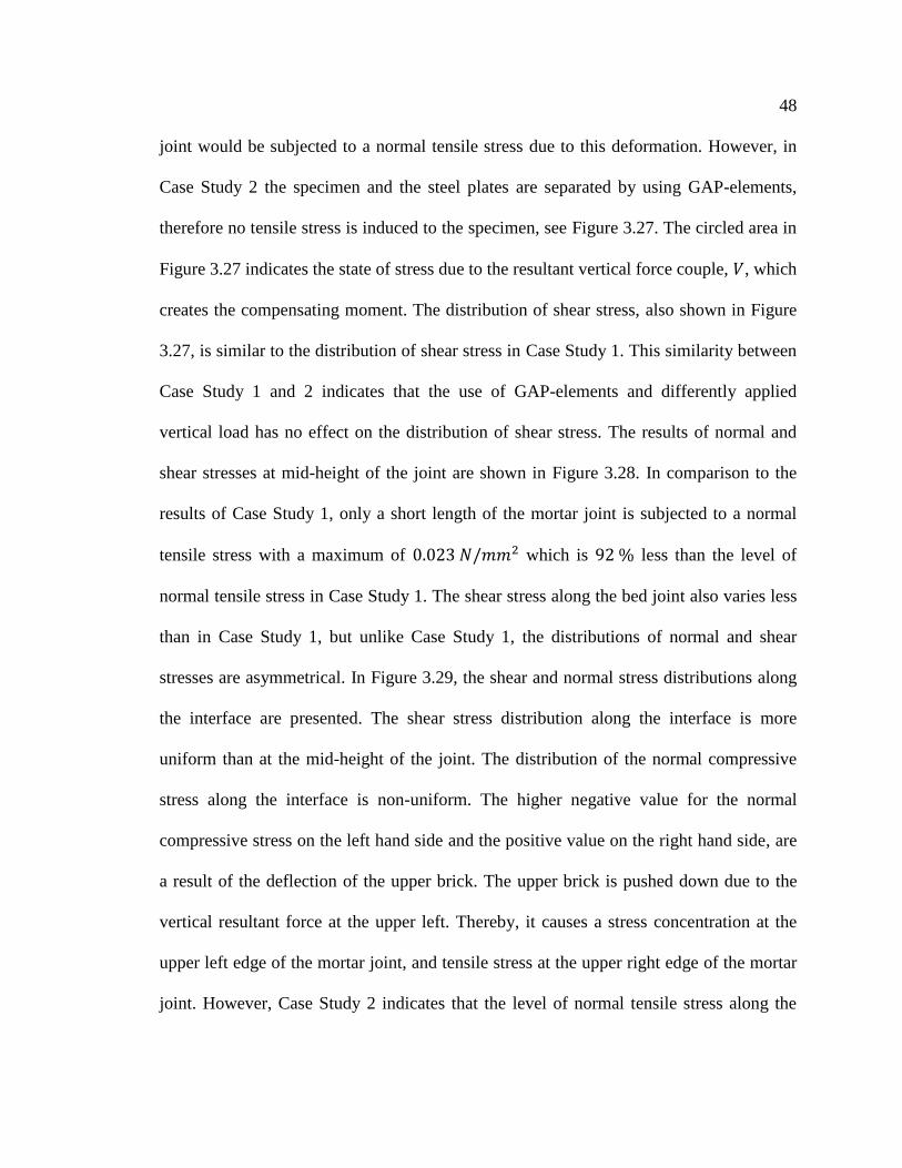
48
joint would be subjected to a normal tensile stress due to this deformation. However, in
Case Study 2 the specimen and the steel plates are separated by using GAP-elements,
therefore no tensile stress is induced to the specimen, see Figure 3.27. The circled area in
Figure 3.27 indicates the state of stress due to the resultant vertical force couple, , which
creates the compensating moment. The distribution of shear stress, also shown in Figure
3.27, is similar to the distribution of shear stress in Case Study 1. This similarity between
Case Study 1 and 2 indicates that the use of GAP-elements and differently applied
vertical load has no effect on the distribution of shear stress. The results of normal and
shear stresses at mid-height of the joint are shown in Figure 3.28. In comparison to the
results of Case Study 1, only a short length of the mortar joint is subjected to a normal
tensile stress with a maximum of which is less than the level of
normal tensile stress in Case Study 1. The shear stress along the bed joint also varies less
than in Case Study 1, but unlike Case Study 1, the distributions of normal and shear
stresses are asymmetrical. In Figure 3.29, the shear and normal stress distributions along
the interface are presented. The shear stress distribution along the interface is more
uniform than at the mid-height of the joint. The distribution of the normal compressive
stress along the interface is non-uniform. The higher negative value for the normal
compressive stress on the left hand side and the positive value on the right hand side, are
a result of the deflection of the upper brick. The upper brick is pushed down due to the
vertical resultant force at the upper left. Thereby, it causes a stress concentration at the
upper left edge of the mortar joint, and tensile stress at the upper right edge of the mortar
joint. However, Case Study 2 indicates that the level of normal tensile stress along the
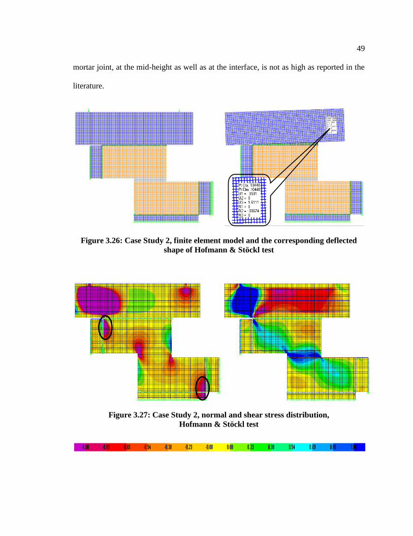
49
mortar joint, at the mid-height as well as at the interface, is not as high as reported in the
literature.
Figure 3.26: Case Study 2, finite element model and the corresponding deflected
shape of Hofmann & Stöckl test
Figure 3.27: Case Study 2, normal and shear stress distribution,
Hofmann & Stöckl test
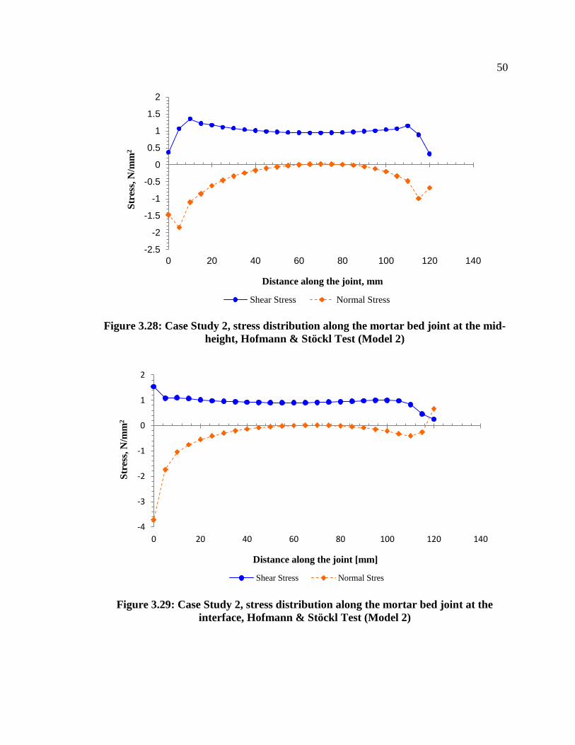
50
Figure 3.28: Case Study 2, stress distribution along the mortar bed joint at the mid-
height, Hofmann & Stöckl Test (Model 2)
Figure 3.29: Case Study 2, stress distribution along the mortar bed joint at the
interface, Hofmann & Stöckl Test (Model 2)
-2.5
-2
-1.5
-1
-0.5
0
0.5
1
1.5
2
0 20 40 60 80 100 120 140
Str
ess,
N/m
m2
Distance along the joint, mm
Shear Stress Normal Stress
-4
-3
-2
-1
0
1
2
0 20 40 60 80 100 120 140
Str
ess,
N/m
m2
Distance along the joint [mm]
Shear Stress Normal Stres
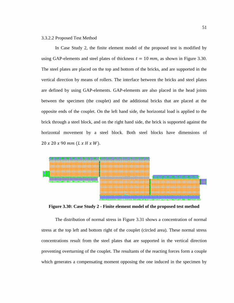
51
3.3.2.2 Proposed Test Method
In Case Study 2, the finite element model of the proposed test is modified by
using GAP-elements and steel plates of thickness , as shown in Figure 3.30.
The steel plates are placed on the top and bottom of the bricks, and are supported in the
vertical direction by means of rollers. The interface between the bricks and steel plates
are defined by using GAP-elements. GAP-elements are also placed in the head joints
between the specimen (the couplet) and the additional bricks that are placed at the
opposite ends of the couplet. On the left hand side, the horizontal load is applied to the
brick through a steel block, and on the right hand side, the brick is supported against the
horizontal movement by a steel block. Both steel blocks have dimensions of
( ).
Figure 3.30: Case Study 2 - Finite element model of the proposed test method
The distribution of normal stress in Figure 3.31 shows a concentration of normal
stress at the top left and bottom right of the couplet (circled area). These normal stress
concentrations result from the steel plates that are supported in the vertical direction
preventing overturning of the couplet. The resultants of the reacting forces form a couple
which generates a compensating moment opposing the one induced in the specimen by
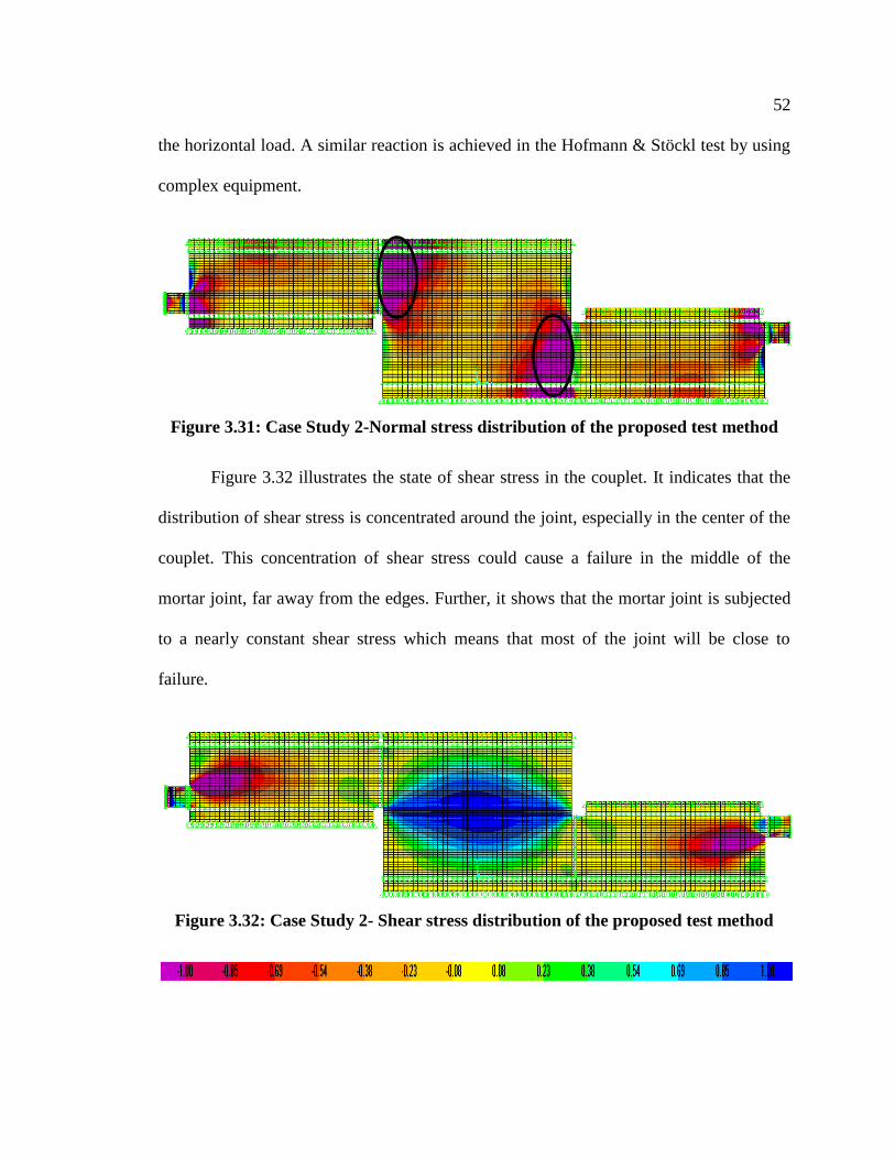
52
the horizontal load. A similar reaction is achieved in the Hofmann & Stöckl test by using
complex equipment.
Figure 3.31: Case Study 2-Normal stress distribution of the proposed test method
Figure 3.32 illustrates the state of shear stress in the couplet. It indicates that the
distribution of shear stress is concentrated around the joint, especially in the center of the
couplet. This concentration of shear stress could cause a failure in the middle of the
mortar joint, far away from the edges. Further, it shows that the mortar joint is subjected
to a nearly constant shear stress which means that most of the joint will be close to
failure.
Figure 3.32: Case Study 2- Shear stress distribution of the proposed test method
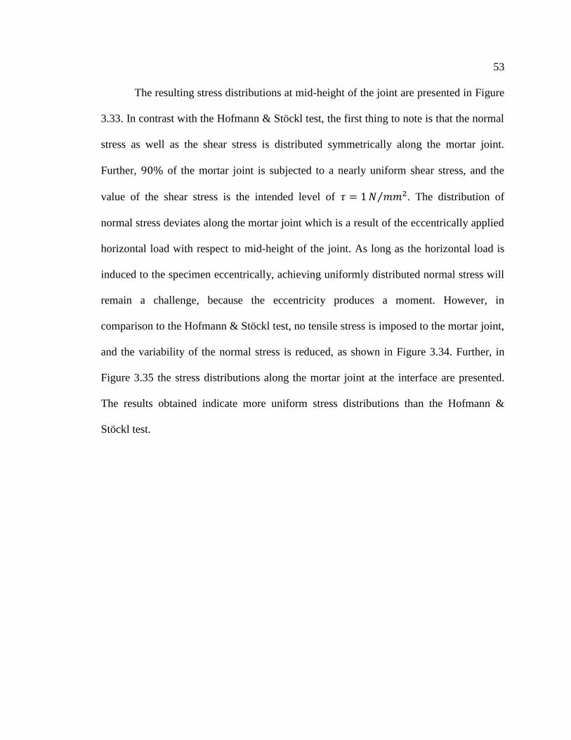
53
The resulting stress distributions at mid-height of the joint are presented in Figure
3.33. In contrast with the Hofmann & Stöckl test, the first thing to note is that the normal
stress as well as the shear stress is distributed symmetrically along the mortar joint.
Further, of the mortar joint is subjected to a nearly uniform shear stress, and the
value of the shear stress is the intended level of ⁄ . The distribution of
normal stress deviates along the mortar joint which is a result of the eccentrically applied
horizontal load with respect to mid-height of the joint. As long as the horizontal load is
induced to the specimen eccentrically, achieving uniformly distributed normal stress will
remain a challenge, because the eccentricity produces a moment. However, in
comparison to the Hofmann & Stöckl test, no tensile stress is imposed to the mortar joint,
and the variability of the normal stress is reduced, as shown in Figure 3.34. Further, in
Figure 3.35 the stress distributions along the mortar joint at the interface are presented.
The results obtained indicate more uniform stress distributions than the Hofmann &
Stöckl test.
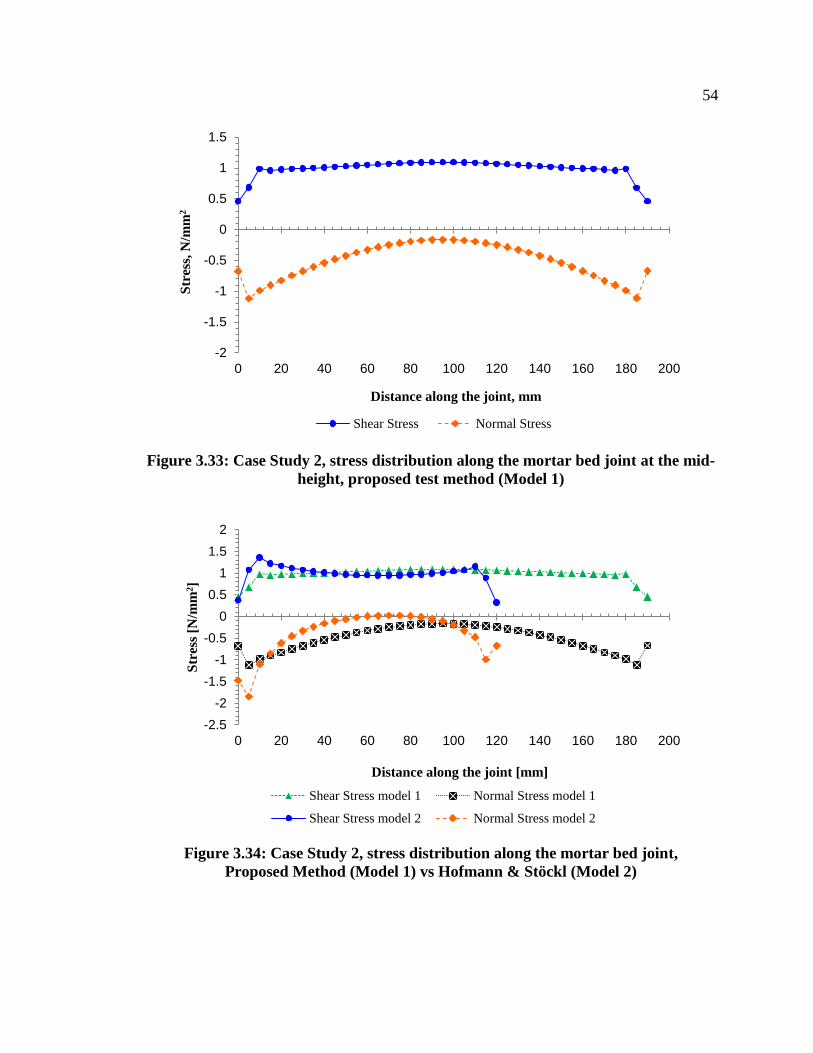
54
Figure 3.33: Case Study 2, stress distribution along the mortar bed joint at the mid-
height, proposed test method (Model 1)
Figure 3.34: Case Study 2, stress distribution along the mortar bed joint,
Proposed Method (Model 1) vs Hofmann & Stöckl (Model 2)
-2
-1.5
-1
-0.5
0
0.5
1
1.5
0 20 40 60 80 100 120 140 160 180 200
Str
ess,
N/m
m2
Distance along the joint, mm
Shear Stress Normal Stress
-2.5
-2
-1.5
-1
-0.5
0
0.5
1
1.5
2
0 20 40 60 80 100 120 140 160 180 200
Str
ess
[N/m
m2]
Distance along the joint [mm]
Shear Stress model 1 Normal Stress model 1
Shear Stress model 2 Normal Stress model 2
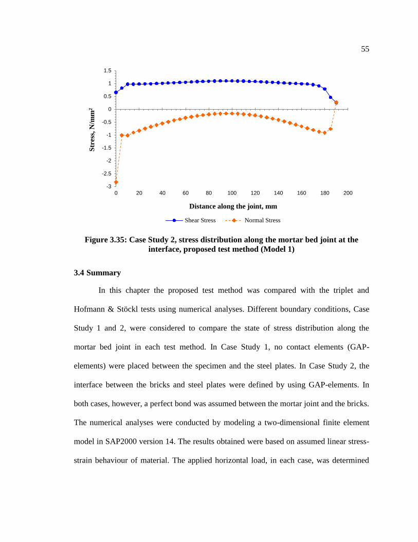
55
Figure 3.35: Case Study 2, stress distribution along the mortar bed joint at the
interface, proposed test method (Model 1)
3.4 Summary
In this chapter the proposed test method was compared with the triplet and
Hofmann & Stöckl tests using numerical analyses. Different boundary conditions, Case
Study 1 and 2, were considered to compare the state of stress distribution along the
mortar bed joint in each test method. In Case Study 1, no contact elements (GAP-
elements) were placed between the specimen and the steel plates. In Case Study 2, the
interface between the bricks and steel plates were defined by using GAP-elements. In
both cases, however, a perfect bond was assumed between the mortar joint and the bricks.
The numerical analyses were conducted by modeling a two-dimensional finite element
model in SAP2000 version 14. The results obtained were based on assumed linear stress-
strain behaviour of material. The applied horizontal load, in each case, was determined
-3
-2.5
-2
-1.5
-1
-0.5
0
0.5
1
1.5
0 20 40 60 80 100 120 140 160 180 200
Str
ess,
N/m
m2
Distance along the joint, mm
Shear Stress Normal Stress
56
with respect to the bed joint area of each specimen to produce an average shear stress of
⁄ .
Based on the numerical evaluations, it can be concluded that the proposed test
method is capable of producing desirable results for nearly uniform shear stress in a
mortar joint. Compared to the triplet test, the resulting distributions of normal and shear
stress in the proposed test method are more uniform, and are based only on one mortar
joint, rather than two as in the triplet test. Further, unlike the case of the triplet test, no
tensile stress is induced in the bed joint. Compared to the Hofmann & Stöckl test, the
distribution of shear stress in the proposed test method is similar; however, the mortar
bed joint is subjected only to normal compressive stress. In Case Study 2, however, it was
demonstrated that by using GAP-elements and differently applied vertical load, the
magnitude of the normal tensile stress in the Hofmann & Stöckl test is not as high as that
reported in the literature.
By using units of different dimensions in the numerical analyses, it was shown that the
results of the Hofmann & Stöckl test as well as the proposed test method are affected by
the length to height ratio of the bricks.
57
CHAPTER 4: EXPERIMENTAL STUDY
4.1 Introduction
The purpose of the numerical evaluation, described in Chapter 3, was to gain
insight into the state of stresses imposed in the mortar bed joint and to compare the
proposed test method with the existing triplet and Hofmann & Stöckl tests. The
evaluation conducted indicates that the proposed test method provides more uniform
distribution for normal and shear stress along the mortar bed joint than the triplet test and
similar results to the Hofmann & Stöckl test.
This chapter provides a detailed description of the proposed test method utilized
for the experimental program, which was intended to verify the results of the numerical
analyses in terms of the state of stress induced in the joint. A description of the materials,
the specimens, and the equipment used for measuring purposes as well as the
experimental program itself is provided here.
4.2 Experimental Program
The purpose of the experimental program was to:
1. Investigate the level of normal and shear stresses induced in the specimen
using the proposed test method.
2. Investigate the consistency of the results obtained using the proposed test
method.
58
The experimental program was conducted using couplet specimens, constructed
using two bricks in stack bond. The specimens were constructed using two types of brick
and one type of mortar. Each combination of brick and mortar was used to produce 25
specimens. During the test procedure, each specimen was subjected to a horizontal load
and to one of the predefined levels of normal compressive stress. In total, four different
levels of pre-compressive stress were combined with the applied horizontal load; and
each combination was tested with five repetitions. Twenty specimens of each
combination were used to investigate the reproducibility of the results using the new test
arrangement. The remaining five specimens of each combination were used in
combination with a digital imaging measurement system to investigate the level of
stresses induced in the specimens in the new test method.
4.3 Development of the Proposed Test Method
The proposed test method is the result of an attempt to combine the advantages of
two existing test methods, namely: the triplet and the Hofmann & Stöckl test. In order to
do so, the proposed test method should utilize simple equipment as in the triplet test, and
it should provide results as good as the Hofmann & Stöckl test (i.e. uniform stresses in
the joint). To fulfill the objectives, a test setup was devised and analyzed by using the
finite element method. The initial numerical analyses of the first test arrangement and the
corresponding results were presented in Popal & Lissel (2010). The first version of the
proposed test arrangement is shown in Figure 4.1.
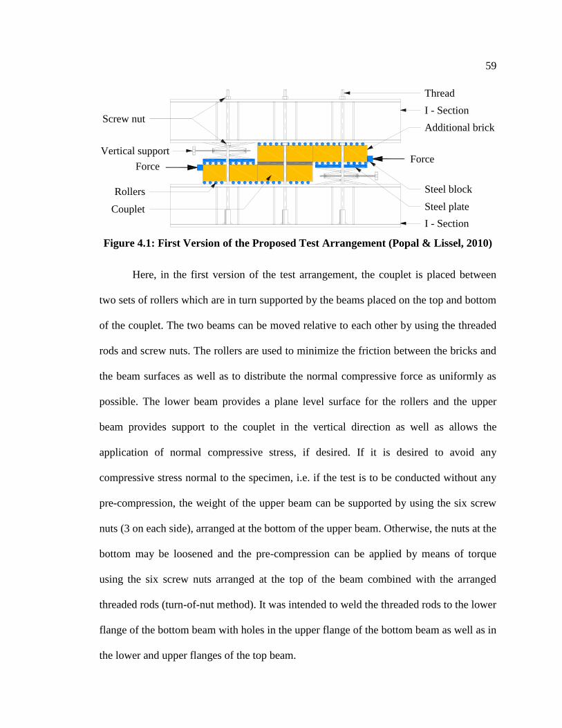
59
Figure 4.1: First Version of the Proposed Test Arrangement (Popal & Lissel, 2010)
Here, in the first version of the test arrangement, the couplet is placed between
two sets of rollers which are in turn supported by the beams placed on the top and bottom
of the couplet. The two beams can be moved relative to each other by using the threaded
rods and screw nuts. The rollers are used to minimize the friction between the bricks and
the beam surfaces as well as to distribute the normal compressive force as uniformly as
possible. The lower beam provides a plane level surface for the rollers and the upper
beam provides support to the couplet in the vertical direction as well as allows the
application of normal compressive stress, if desired. If it is desired to avoid any
compressive stress normal to the specimen, i.e. if the test is to be conducted without any
pre-compression, the weight of the upper beam can be supported by using the six screw
nuts (3 on each side), arranged at the bottom of the upper beam. Otherwise, the nuts at the
bottom may be loosened and the pre-compression can be applied by means of torque
using the six screw nuts arranged at the top of the beam combined with the arranged
threaded rods (turn-of-nut method). It was intended to weld the threaded rods to the lower
flange of the bottom beam with holes in the upper flange of the bottom beam as well as in
the lower and upper flanges of the top beam.
I - Section
Additional brick
Thread
I - Section
Steel block
Steel plate
Force
Screw nut
Rollers
Force
Vertical support
Couplet
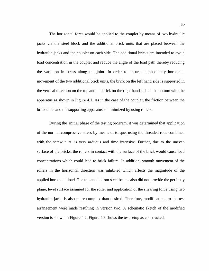
60
The horizontal force would be applied to the couplet by means of two hydraulic
jacks via the steel block and the additional brick units that are placed between the
hydraulic jacks and the couplet on each side. The additional bricks are intended to avoid
load concentration in the couplet and reduce the angle of the load path thereby reducing
the variation in stress along the joint. In order to ensure an absolutely horizontal
movement of the two additional brick units, the brick on the left hand side is supported in
the vertical direction on the top and the brick on the right hand side at the bottom with the
apparatus as shown in Figure 4.1. As in the case of the couplet, the friction between the
brick units and the supporting apparatus is minimized by using rollers.
During the initial phase of the testing program, it was determined that application
of the normal compressive stress by means of torque, using the threaded rods combined
with the screw nuts, is very arduous and time intensive. Further, due to the uneven
surface of the bricks, the rollers in contact with the surface of the brick would cause load
concentrations which could lead to brick failure. In addition, smooth movement of the
rollers in the horizontal direction was inhibited which affects the magnitude of the
applied horizontal load. The top and bottom steel beams also did not provide the perfectly
plane, level surface assumed for the roller and application of the shearing force using two
hydraulic jacks is also more complex than desired. Therefore, modifications to the test
arrangement were made resulting in version two. A schematic sketch of the modified
version is shown in Figure 4.2. Figure 4.3 shows the test setup as constructed.
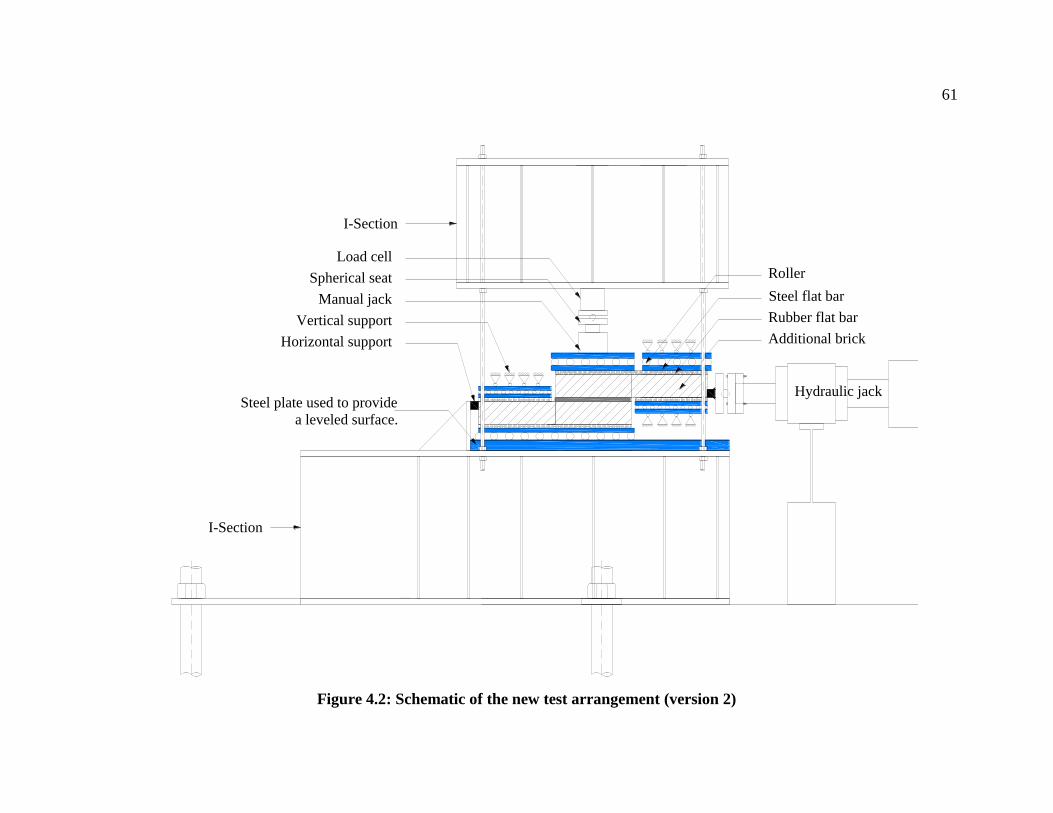
61
Figure 4.2: Schematic of the new test arrangement (version 2)
Roller
Steel flat bar
Rubber flat bar
I-Section
Hydraulic jack
Additional brick
Steel plate used to provide
a leveled surface.
Load cell
Horizontal support
Manual jack
Vertical support
Spherical seat
I-Section
62
Figure 4.3: Test arrangement for version 2 of the proposed test method
Here, a plane, level surface for the rollers is provided by means of a steel plate
with smoothed surface and dimensions of . The steel plate is bedded
on the top of the lower beam by means of leveling grout (plaster of Paris). In addition to
the steel plate, a horizontal support is welded on top of the lower beam, and thereby one
of the hydraulic jacks is replaced. The reaction load at the horizontal support is
transferred by the lower beam to the floor by fixing the beam to the floor. This ensures
that the results obtained due to the horizontal load are not affected by load circulation in
the test setup. Further, the normal compressive stress is applied to the specimen by using
a manually operated jack instead of torqueing the screw nuts on the threaded rods. The
63
normal compressive force is measured by a load cell placed on top of a spherical seat
between the upper beam and manually operated jack. The equivalent vertical load for
each level of intended compressive stress was determined based on the nominal area of
the gross bedded area of the units. In this modified test arrangement, the upper beam
provides a rigid surface in the vertical direction and support for the manually operated
jack, and the lower beam, as before, is fixed to the floor and provides a level, plane
surface as well as support in the horizontal direction.
During this redesign phase, the use of Teflon sheets instead of rollers was also
considered. The recommended product is composed of two Teflon sheets (each with a
thickness of and a coefficient of friction of ) and two rubber
sheets (each with a thickness of ), and is manufactured in the Netherlands.
The layers are stacked as follows: One layer rubber followed by two layers of Teflon
sheet and an additional layer of rubber on the top of it. However, the material could not
be shipped outside Europe and an equivalent material was not available in North
America. Therefore the idea was replaced by using an assembly composed of one sheet
of rubber, , one steel plate ( ), and one roller with repeating steel
plate and rubber sheet on the top of it. The rubber sheets are used to accommodate the
unevenness of the surface of the bricks and the steel plates are used to allow smooth
movement of the rollers. The steel plates arranged at the top and bottom of the couplet
are not connected to the plates arranged at the top and bottom of the additional bricks, so
that the couplet and the additional brick can move independently.
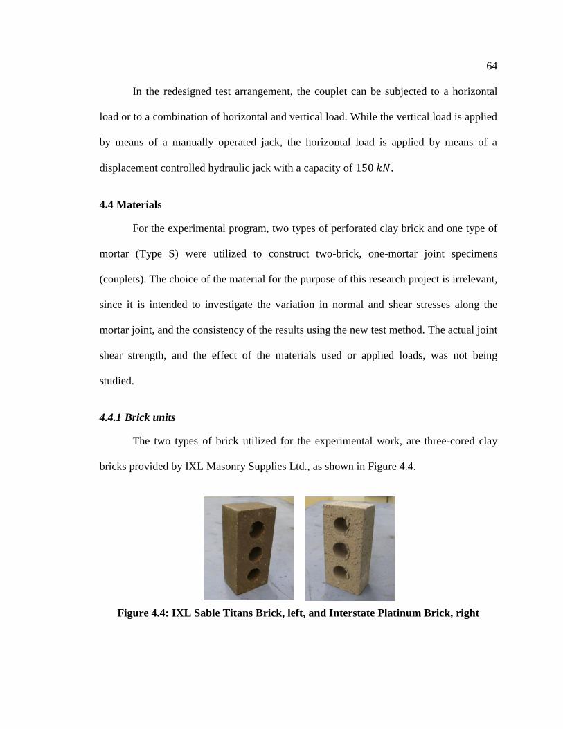
64
In the redesigned test arrangement, the couplet can be subjected to a horizontal
load or to a combination of horizontal and vertical load. While the vertical load is applied
by means of a manually operated jack, the horizontal load is applied by means of a
displacement controlled hydraulic jack with a capacity of .
4.4 Materials
For the experimental program, two types of perforated clay brick and one type of
mortar (Type S) were utilized to construct two-brick, one-mortar joint specimens
(couplets). The choice of the material for the purpose of this research project is irrelevant,
since it is intended to investigate the variation in normal and shear stresses along the
mortar joint, and the consistency of the results using the new test method. The actual joint
shear strength, and the effect of the materials used or applied loads, was not being
studied.
4.4.1 Brick units
The two types of brick utilized for the experimental work, are three-cored clay
bricks provided by IXL Masonry Supplies Ltd., as shown in Figure 4.4.
Figure 4.4: IXL Sable Titans Brick, left, and Interstate Platinum Brick, right
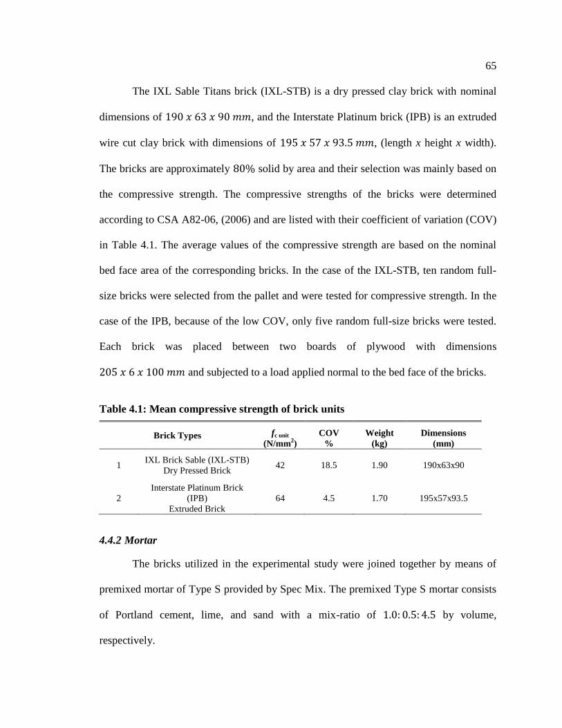
65
The IXL Sable Titans brick (IXL-STB) is a dry pressed clay brick with nominal
dimensions of , and the Interstate Platinum brick (IPB) is an extruded
wire cut clay brick with dimensions of , (length x height x width).
The bricks are approximately solid by area and their selection was mainly based on
the compressive strength. The compressive strengths of the bricks were determined
according to CSA A82-06, (2006) and are listed with their coefficient of variation (COV)
in Table 4.1. The average values of the compressive strength are based on the nominal
bed face area of the corresponding bricks. In the case of the IXL-STB, ten random full-
size bricks were selected from the pallet and were tested for compressive strength. In the
case of the IPB, because of the low COV, only five random full-size bricks were tested.
Each brick was placed between two boards of plywood with dimensions
and subjected to a load applied normal to the bed face of the bricks.
Table 4.1: Mean compressive strength of brick units
Brick Types fc unit
(N/mm2)
COV
%
Weight
(kg)
Dimensions
(mm)
1 IXL Brick Sable (IXL-STB)
Dry Pressed Brick 42 18.5 1.90 190x63x90
2
Interstate Platinum Brick
(IPB)
Extruded Brick
64 4.5 1.70 195x57x93.5
4.4.2 Mortar
The bricks utilized in the experimental study were joined together by means of
premixed mortar of Type S provided by Spec Mix. The premixed Type S mortar consists
of Portland cement, lime, and sand with a mix-ratio of by volume,
respectively.
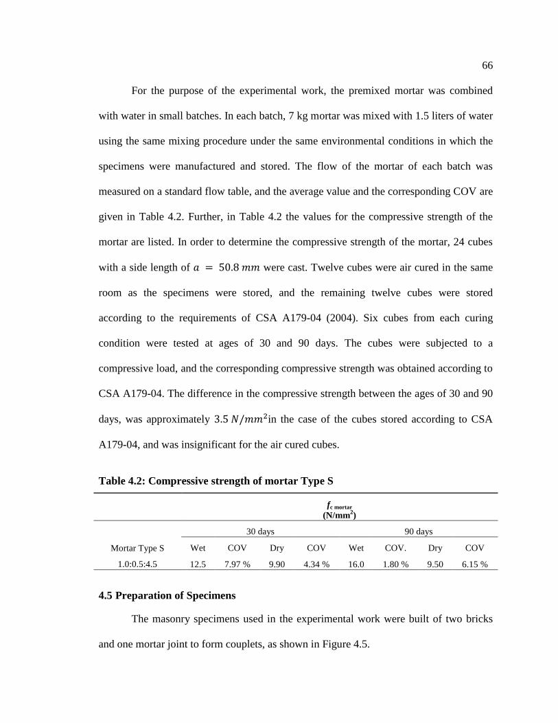
66
For the purpose of the experimental work, the premixed mortar was combined
with water in small batches. In each batch, 7 kg mortar was mixed with 1.5 liters of water
using the same mixing procedure under the same environmental conditions in which the
specimens were manufactured and stored. The flow of the mortar of each batch was
measured on a standard flow table, and the average value and the corresponding COV are
given in Table 4.2. Further, in Table 4.2 the values for the compressive strength of the
mortar are listed. In order to determine the compressive strength of the mortar, 24 cubes
with a side length of were cast. Twelve cubes were air cured in the same
room as the specimens were stored, and the remaining twelve cubes were stored
according to the requirements of CSA A179-04 (2004). Six cubes from each curing
condition were tested at ages of 30 and 90 days. The cubes were subjected to a
compressive load, and the corresponding compressive strength was obtained according to
CSA A179-04. The difference in the compressive strength between the ages of 30 and 90
days, was approximately in the case of the cubes stored according to CSA
A179-04, and was insignificant for the air cured cubes.
Table 4.2: Compressive strength of mortar Type S
fc mortar
(N/mm2)
30 days 90 days
Mortar Type S
1.0:0.5:4.5
Wet COV Dry COV Wet COV. Dry COV
12.5 7.97 % 9.90 4.34 % 16.0 1.80 % 9.50 6.15 %
4.5 Preparation of Specimens
The masonry specimens used in the experimental work were built of two bricks
and one mortar joint to form couplets, as shown in Figure 4.5.
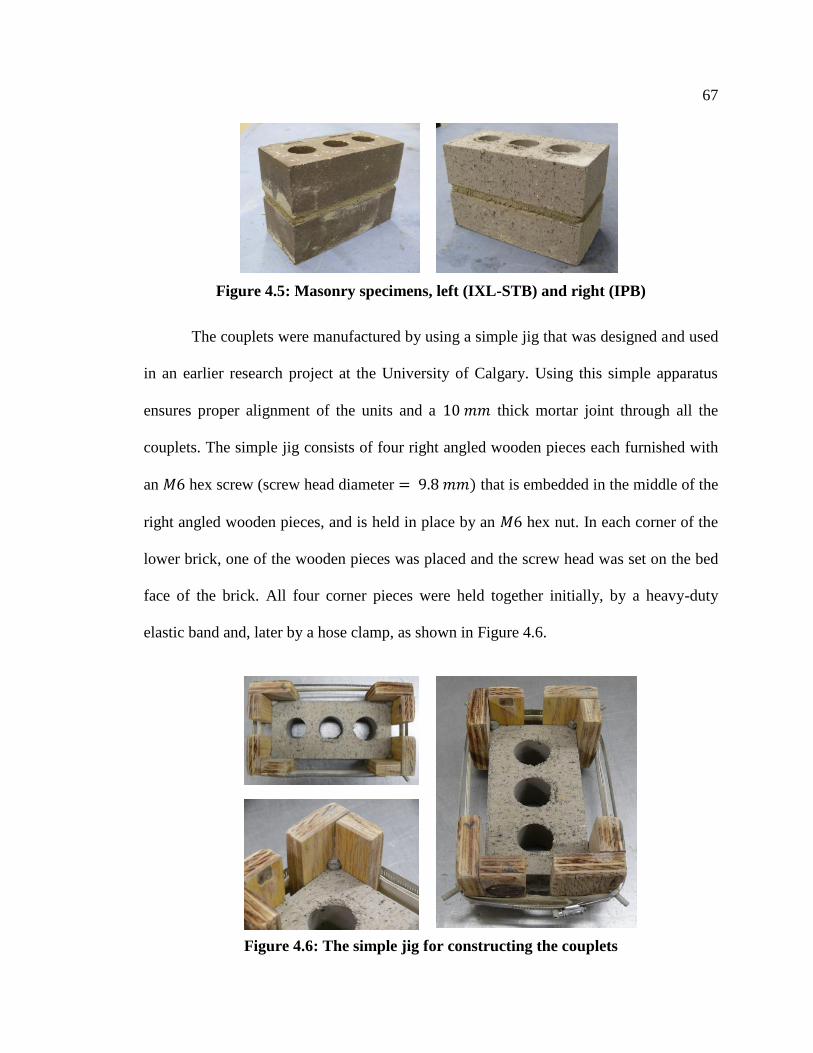
67
Figure 4.5: Masonry specimens, left (IXL-STB) and right (IPB)
The couplets were manufactured by using a simple jig that was designed and used
in an earlier research project at the University of Calgary. Using this simple apparatus
ensures proper alignment of the units and a thick mortar joint through all the
couplets. The simple jig consists of four right angled wooden pieces each furnished with
an hex screw (screw head diameter ) that is embedded in the middle of the
right angled wooden pieces, and is held in place by an hex nut. In each corner of the
lower brick, one of the wooden pieces was placed and the screw head was set on the bed
face of the brick. All four corner pieces were held together initially, by a heavy-duty
elastic band and, later by a hose clamp, as shown in Figure 4.6.
Figure 4.6: The simple jig for constructing the couplets
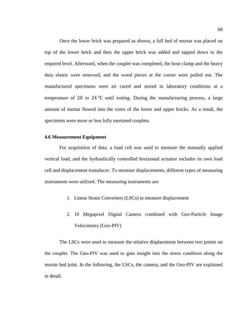
68
Once the lower brick was prepared as shown, a full bed of mortar was placed on
top of the lower brick and then the upper brick was added and tapped down to the
required level. Afterward, when the couplet was completed, the hose clamp and the heavy
duty elastic were removed, and the wood pieces at the corner were pulled out. The
manufactured specimens were air cured and stored in laboratory conditions at a
temperature of to until testing. During the manufacturing process, a large
amount of mortar flowed into the cores of the lower and upper bricks. As a result, the
specimens were more or less fully mortared couplets.
4.6 Measurement Equipment
For acquisition of data, a load cell was used to measure the manually applied
vertical load, and the hydraulically controlled horizontal actuator includes its own load
cell and displacement transducer. To measure displacements, different types of measuring
instruments were utilized. The measuring instruments are:
1. Linear Strain Converters (LSCs) to measure displacement
2. 10 Megapixel Digital Camera combined with Geo-Particle Image
Velocimetry (Geo-PIV)
The LSCs were used to measure the relative displacement between two points on
the couplet. The Geo-PIV was used to gain insight into the stress condition along the
mortar bed joint. In the following, the LSCs, the camera, and the Geo-PIV are explained
in detail.
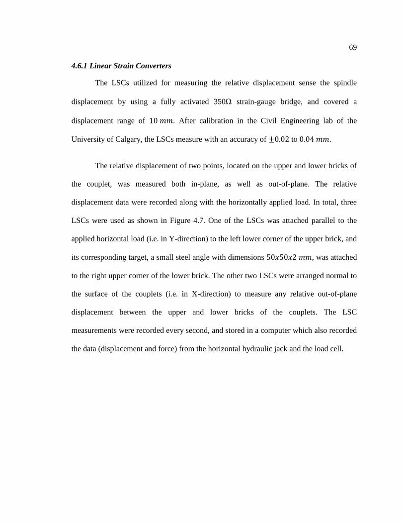
69
4.6.1 Linear Strain Converters
The LSCs utilized for measuring the relative displacement sense the spindle
displacement by using a fully activated 350 strain-gauge bridge, and covered a
displacement range of . After calibration in the Civil Engineering lab of the
University of Calgary, the LSCs measure with an accuracy of to .
The relative displacement of two points, located on the upper and lower bricks of
the couplet, was measured both in-plane, as well as out-of-plane. The relative
displacement data were recorded along with the horizontally applied load. In total, three
LSCs were used as shown in Figure 4.7. One of the LSCs was attached parallel to the
applied horizontal load (i.e. in Y-direction) to the left lower corner of the upper brick, and
its corresponding target, a small steel angle with dimensions , was attached
to the right upper corner of the lower brick. The other two LSCs were arranged normal to
the surface of the couplets (i.e. in X-direction) to measure any relative out-of-plane
displacement between the upper and lower bricks of the couplets. The LSC
measurements were recorded every second, and stored in a computer which also recorded
the data (displacement and force) from the horizontal hydraulic jack and the load cell.
70
Figure 4.7: Arrangement of LSCs on the specimens
4.6.2 Particle Image Velocimetry and GeoPIV
A Particle Image Velocimety (PIV) system of measurement uses images of
particles to measure the flow velocity. The technique was originally developed in the
field of fluid mechanics, and was utilized for measuring flow field in a fluid (Adrian,
1991). In the PIV technique, this is done by tracking patches placed in an area of interest
through a series of digitally captured images. Later, once a series of digital images is
captured, the area of interest in the initial image can be divided in a mesh of PIV test
patches. Each patch possesses a unique texture and specific coordinates in image at the
time , ( ). To locate the specific coordinates of a patch from image within a
corresponding pre-defined larger search patch in image , the correlation between the two
patches is evaluated. The location with the highest correlation within the search patch
indicates the specific coordinates of the initial patch at time in image , ( ).
This procedure, as illustrated in Figure 4.8, is repeated for the entire mesh of patches
within an image, and then repeated for each image within the series, to determine the
displacement vector of each test patch (White & Take, 2002).
LSCs
Target
Y
Z
X
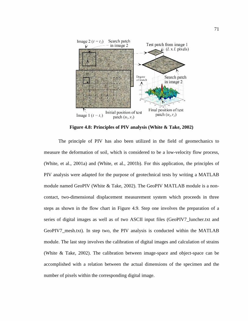
71
Figure 4.8: Principles of PIV analysis (White & Take, 2002)
The principle of PIV has also been utilized in the field of geomechanics to
measure the deformation of soil, which is considered to be a low-velocity flow process,
(White, et al., 2001a) and (White, et al., 2001b). For this application, the principles of
PIV analysis were adapted for the purpose of geotechnical tests by writing a MATLAB
module named GeoPIV (White & Take, 2002). The GeoPIV MATLAB module is a non-
contact, two-dimensional displacement measurement system which proceeds in three
steps as shown in the flow chart in Figure 4.9. Step one involves the preparation of a
series of digital images as well as of two ASCII input files (GeoPIV7_luncher.txt and
GeoPIV7_mesh.txt). In step two, the PIV analysis is conducted within the MATLAB
module. The last step involves the calibration of digital images and calculation of strains
(White & Take, 2002). The calibration between image-space and object-space can be
accomplished with a relation between the actual dimensions of the specimen and the
number of pixels within the corresponding digital image.
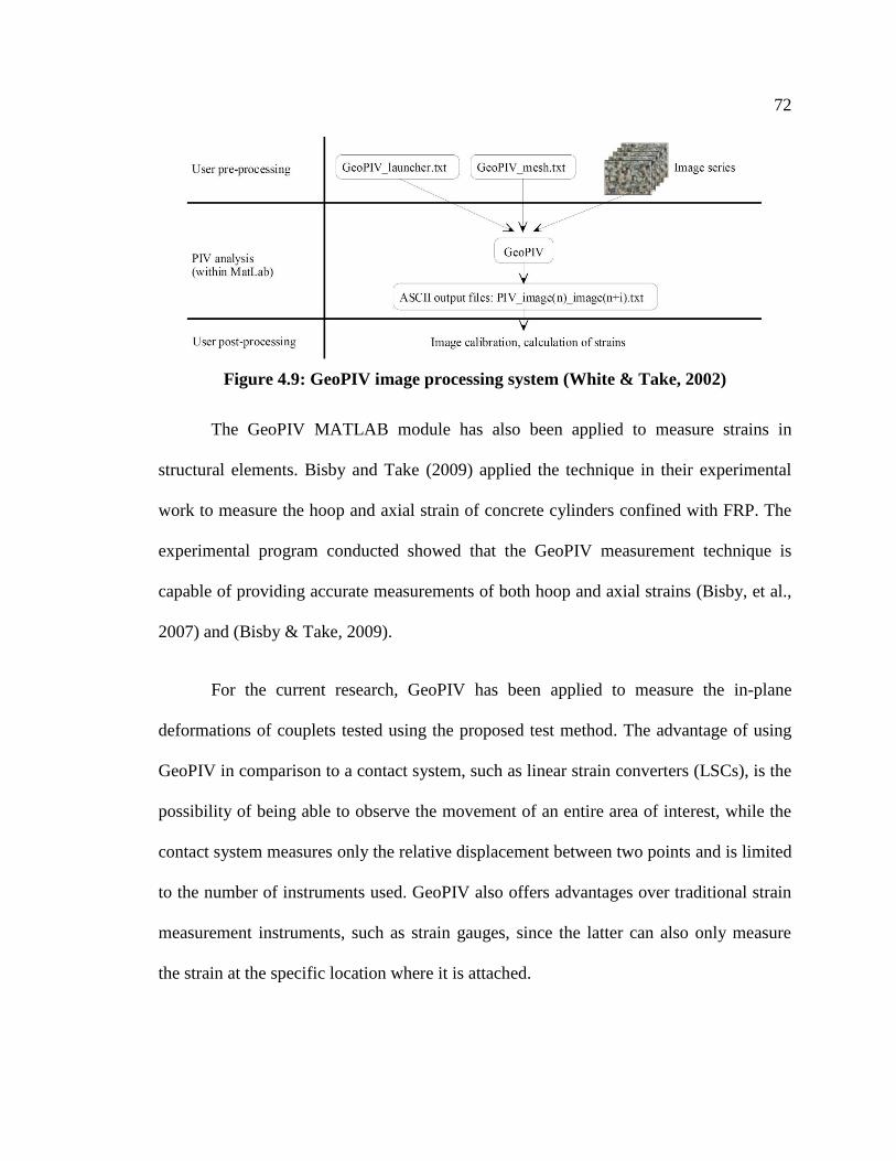
72
Figure 4.9: GeoPIV image processing system (White & Take, 2002)
The GeoPIV MATLAB module has also been applied to measure strains in
structural elements. Bisby and Take (2009) applied the technique in their experimental
work to measure the hoop and axial strain of concrete cylinders confined with FRP. The
experimental program conducted showed that the GeoPIV measurement technique is
capable of providing accurate measurements of both hoop and axial strains (Bisby, et al.,
2007) and (Bisby & Take, 2009).
For the current research, GeoPIV has been applied to measure the in-plane
deformations of couplets tested using the proposed test method. The advantage of using
GeoPIV in comparison to a contact system, such as linear strain converters (LSCs), is the
possibility of being able to observe the movement of an entire area of interest, while the
contact system measures only the relative displacement between two points and is limited
to the number of instruments used. GeoPIV also offers advantages over traditional strain
measurement instruments, such as strain gauges, since the latter can also only measure
the strain at the specific location where it is attached.
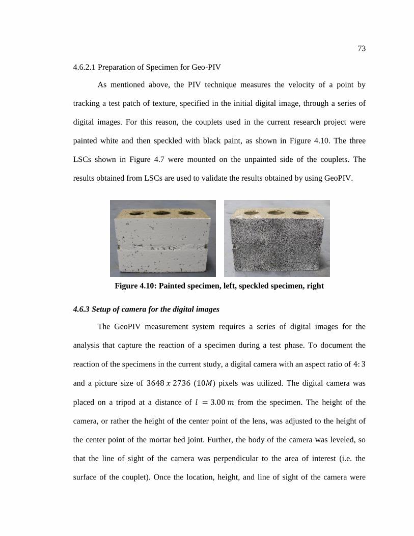
73
4.6.2.1 Preparation of Specimen for Geo-PIV
As mentioned above, the PIV technique measures the velocity of a point by
tracking a test patch of texture, specified in the initial digital image, through a series of
digital images. For this reason, the couplets used in the current research project were
painted white and then speckled with black paint, as shown in Figure 4.10. The three
LSCs shown in Figure 4.7 were mounted on the unpainted side of the couplets. The
results obtained from LSCs are used to validate the results obtained by using GeoPIV.
Figure 4.10: Painted specimen, left, speckled specimen, right
4.6.3 Setup of camera for the digital images
The GeoPIV measurement system requires a series of digital images for the
analysis that capture the reaction of a specimen during a test phase. To document the
reaction of the specimens in the current study, a digital camera with an aspect ratio of
and a picture size of ( ) pixels was utilized. The digital camera was
placed on a tripod at a distance of from the specimen. The height of the
camera, or rather the height of the center point of the lens, was adjusted to the height of
the center point of the mortar bed joint. Further, the body of the camera was leveled, so
that the line of sight of the camera was perpendicular to the area of interest (i.e. the
surface of the couplet). Once the location, height, and line of sight of the camera were
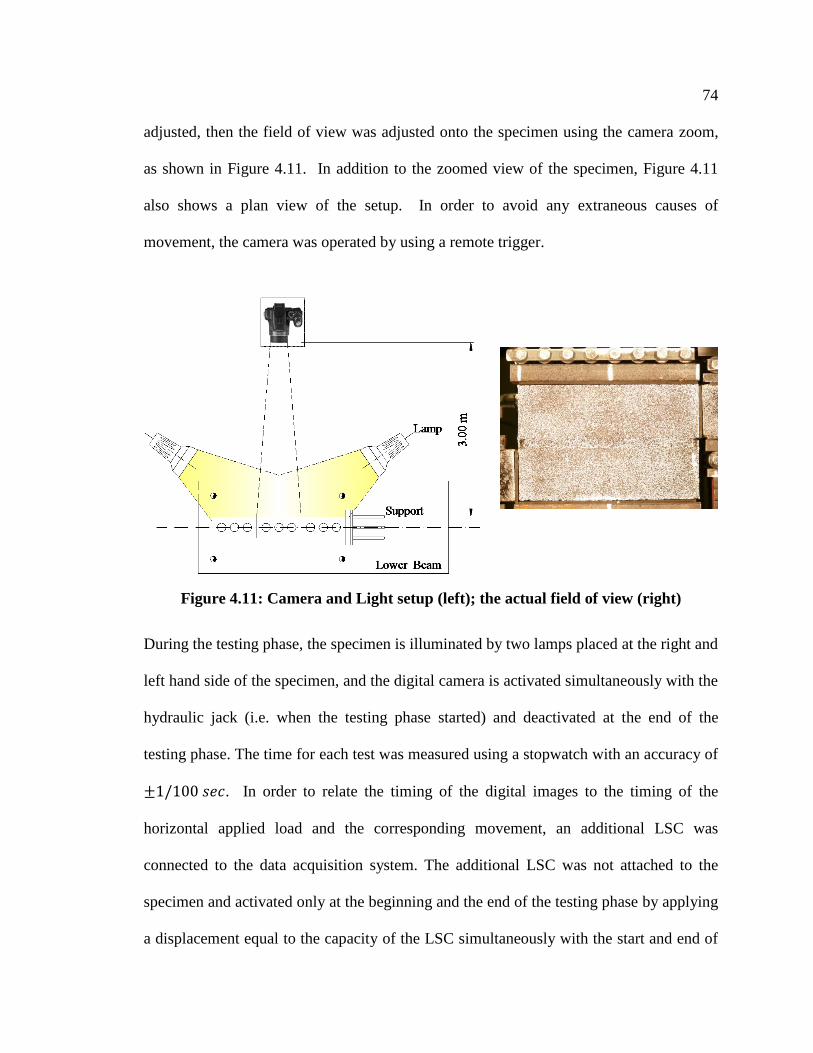
74
adjusted, then the field of view was adjusted onto the specimen using the camera zoom,
as shown in Figure 4.11. In addition to the zoomed view of the specimen, Figure 4.11
also shows a plan view of the setup. In order to avoid any extraneous causes of
movement, the camera was operated by using a remote trigger.
Figure 4.11: Camera and Light setup (left); the actual field of view (right)
During the testing phase, the specimen is illuminated by two lamps placed at the right and
left hand side of the specimen, and the digital camera is activated simultaneously with the
hydraulic jack (i.e. when the testing phase started) and deactivated at the end of the
testing phase. The time for each test was measured using a stopwatch with an accuracy of
. In order to relate the timing of the digital images to the timing of the
horizontal applied load and the corresponding movement, an additional LSC was
connected to the data acquisition system. The additional LSC was not attached to the
specimen and activated only at the beginning and the end of the testing phase by applying
a displacement equal to the capacity of the LSC simultaneously with the start and end of
75
the testing phase. These two measurements mark the exact time of the testing phase in the
recorded data produced by the hydraulic jack.
4.7 Summary
This chapter describes the experimental program, the materials utilized, the
specimens, the measurement equipment, and the arrangement of the proposed test
method. Two types of clay brick (dry-pressed and extruded) and one type of mortar
(Type S) were combined to construct two-brick, one-mortar joint specimens. After
curing, the specimens were tested by using the proposed test method. During the testing
phase, the specimens were subjected to horizontal and vertical loads using a hydraulic
displacement controlled actuator and a manually operated jack, respectively. In total, 50
specimens, 25 for each brick type, were tested at four different levels of pre-compressive
stress normal to the bed joint. The relative displacement between the upper and lower
bricks of the specimen was measured with Linear Strain Converters (LSCs). In addition
to the LSCs, a measurement system based on Particle Images Velocimetry (PIV) was
utilized to gain insight into the state of stresses along the mortar joint and to measure the
displacement of an entire area of interest. The recorded data are summarized, analyzed,
and discussed in Chapter 5.
76
CHAPTER 5: RESULTS AND DISCUSSION
5.1 Introduction
A new test method was proposed, constructed, and used to test 50 couplets
constructed of two types of brick and one type of mortar. The tests conducted were
divided into eight series with varying levels of pre-compression (Series I to Series VIII).
The specimens, test setup and the experimental program with the corresponding load
condition were described in Chapter 4.
In this chapter, the results obtained using conventional Linear Strain Converters
(LSCs), as well as the particle image velocimetry measurement system, GeoPIV, are
presented and discussed. The results obtained using the LSCs were recorded
automatically into a computer every second, and the images for use in the Geo-PIV
software were recorded at a rate of approximately two digital images per second. First,
the load-displacement behaviour observed using the LSCs is presented, followed by the
results from the GeoPIV analysis. The results of the first 40 tests were measured with the
LSCs (Appendix A), and were used to evaluate the reproducibility of results using the
proposed test method. Ten additional tests were carried out with the GeoPIV
measurement system, in addition to the LSCs, and were used to gain insight into the state
of normal and shear stress that is induced in the mortar bed joint using the proposed test
method.
77
5.2 Measurements using Linear Strain Converters
5.2.1 Results
5.2.1.1 IXL-STB (Dry Pressed Brick)
Twenty couplets were divided into four series where a different level of normal
compressive stress ( ) was applied for each series,
with each series consisting of five specimens. To induce the desired level of normal
compressive stress, in Series # I, the specimens were subjected to a normal compressive
load of , in Series # II to a normal compressive load of , in Series # III to a
normal compressive load of , and Series # IV to a normal compressive load of
. Following application of the normal compressive load, the displacement
controlled horizontal load was applied with a speed of . For all
specimens, the horizontal load was applied until failure occurred and until a clear
tendency of the residual strength was observed. The normal compressive force, the
horizontal load, and the relative shearing displacement between the upper and lower
bricks were measured and recorded continuously and automatically once per second.
During the testing, all twenty specimens, subjected to the above mentioned
loading conditions, experienced a small rotation which led to an uplift of about at
the heel of the specimens. No cracking of the mortar joint or debonding of the interface
between the mortar joint and the bricks was observed at the time that the overturning of
the specimens occurred. However, with increasing horizontal load the cracking process
started at the upper interface between the mortar joint and the upper brick at the side
where the horizontal load was applied. The initiated crack continued to propagate along
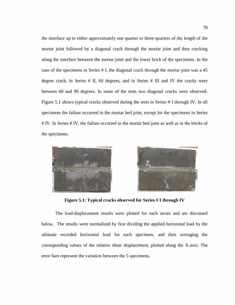
78
the interface up to either approximately one quarter or three-quarters of the length of the
mortar joint followed by a diagonal crack through the mortar joint and then cracking
along the interface between the mortar joint and the lower brick of the specimens. In the
case of the specimens in Series # I, the diagonal crack through the mortar joint was a 45
degree crack, in Series # II, 60 degrees, and in Series # III and IV the cracks were
between 60 and 90 degrees. In some of the tests two diagonal cracks were observed.
Figure 5.1 shows typical cracks observed during the tests in Series # I through IV. In all
specimens the failure occurred in the mortar bed joint, except for the specimens in Series
# IV. In Series # IV, the failure occurred in the mortar bed joint as well as in the bricks of
the specimens.
Figure 5.1: Typical cracks observed for Series # I through IV
The load-displacement results were plotted for each series and are discussed
below. The results were normalized by first dividing the applied horizontal load by the
ultimate recorded horizontal load for each specimen, and then averaging the
corresponding values of the relative shear displacement, plotted along the X-axis. The
error bars represent the variation between the 5 specimens.
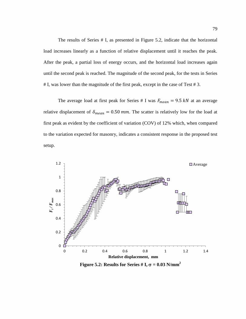
79
The results of Series # I, as presented in Figure 5.2, indicate that the horizontal
load increases linearly as a function of relative displacement until it reaches the peak.
After the peak, a partial loss of energy occurs, and the horizontal load increases again
until the second peak is reached. The magnitude of the second peak, for the tests in Series
# I, was lower than the magnitude of the first peak, except in the case of Test # 3.
The average load at first peak for Series # I was at an average
relative displacement of . The scatter is relatively low for the load at
first peak as evident by the coefficient of variation (COV) of 12% which, when compared
to the variation expected for masonry, indicates a consistent response in the proposed test
setup.
Figure 5.2: Results for Series # I, = 0.03 N/mm
2
0
0.2
0.4
0.6
0.8
1
1.2
0 0.2 0.4 0.6 0.8 1 1.2 1.4
Fi /
Fm
ax
Relative displacement, mm
Average
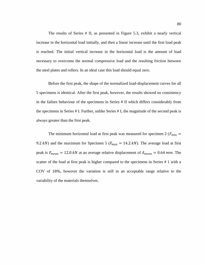
80
The results of Series # II, as presented in Figure 5.3, exhibit a nearly vertical
increase in the horizontal load initially, and then a linear increase until the first load peak
is reached. The initial vertical increase in the horizontal load is the amount of load
necessary to overcome the normal compressive load and the resulting friction between
the steel plates and rollers. In an ideal case this load should equal zero.
Before the first peak, the shape of the normalized load-displacement curves for all
5 specimens is identical. After the first peak, however, the results showed no consistency
in the failure behaviour of the specimens in Series # II which differs considerably from
the specimens in Series # I. Further, unlike Series # I, the magnitude of the second peak is
always greater than the first peak.
The minimum horizontal load at first peak was measured for specimen 2 (
) and the maximum for Specimen 5 ( ). The average load at first
peak is at an average relative displacement of . The
scatter of the load at first peak is higher compared to the specimens in Series # 1 with a
COV of , however the variation is still in an acceptable range relative to the
variability of the materials themselves.
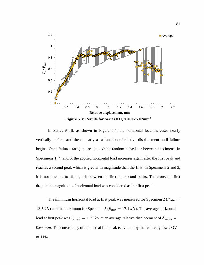
81
Figure 5.3: Results for Series # II, = 0.25 N/mm
2
In Series # III, as shown in Figure 5.4, the horizontal load increases nearly
vertically at first, and then linearly as a function of relative displacement until failure
begins. Once failure starts, the results exhibit random behaviour between specimens. In
Specimens 1, 4, and 5, the applied horizontal load increases again after the first peak and
reaches a second peak which is greater in magnitude than the first. In Specimens 2 and 3,
it is not possible to distinguish between the first and second peaks. Therefore, the first
drop in the magnitude of horizontal load was considered as the first peak.
The minimum horizontal load at first peak was measured for Specimen 2 (
) and the maximum for Specimen 5 ( ). The average horizontal
load at first peak was at an average relative displacement of
. The consistency of the load at first peak is evident by the relatively low COV
of 11%.
0
0.2
0.4
0.6
0.8
1
1.2
0 0.2 0.4 0.6 0.8 1 1.2 1.4 1.6 1.8 2 2.2
Fi /
Fm
ax
Relative displacement, mm
Average
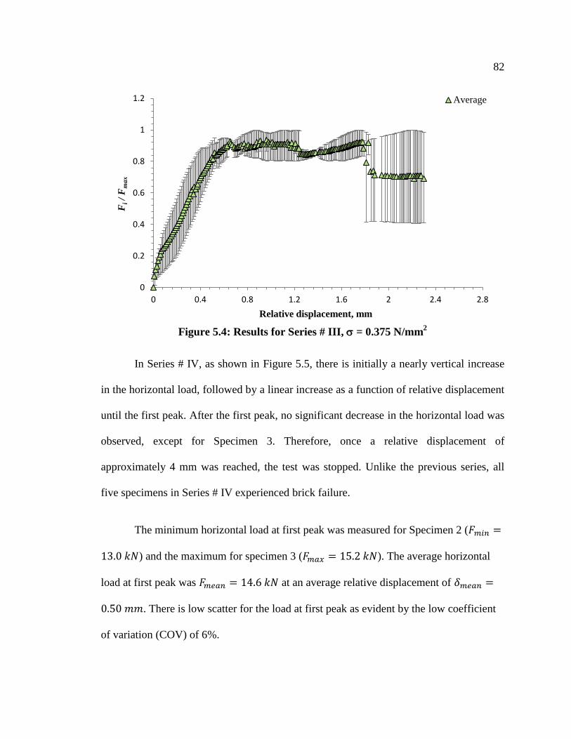
82
Figure 5.4: Results for Series # III, = 0.375 N/mm
2
In Series # IV, as shown in Figure 5.5, there is initially a nearly vertical increase
in the horizontal load, followed by a linear increase as a function of relative displacement
until the first peak. After the first peak, no significant decrease in the horizontal load was
observed, except for Specimen 3. Therefore, once a relative displacement of
approximately 4 mm was reached, the test was stopped. Unlike the previous series, all
five specimens in Series # IV experienced brick failure.
The minimum horizontal load at first peak was measured for Specimen 2 (
) and the maximum for specimen 3 ( ). The average horizontal
load at first peak was at an average relative displacement of
. There is low scatter for the load at first peak as evident by the low coefficient
of variation (COV) of 6%.
0
0.2
0.4
0.6
0.8
1
1.2
0 0.4 0.8 1.2 1.6 2 2.4 2.8
Fi /
Fm
ax
Relative displacement, mm
Average
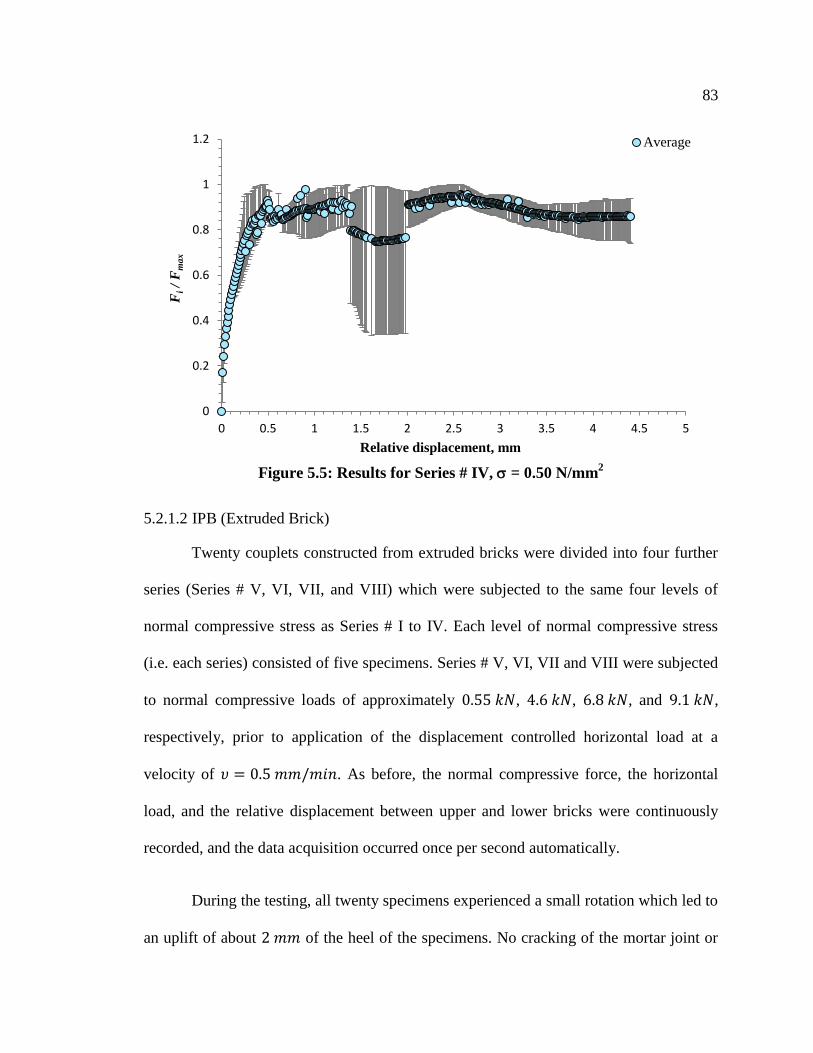
83
Figure 5.5: Results for Series # IV, = 0.50 N/mm
2
5.2.1.2 IPB (Extruded Brick)
Twenty couplets constructed from extruded bricks were divided into four further
series (Series # V, VI, VII, and VIII) which were subjected to the same four levels of
normal compressive stress as Series # I to IV. Each level of normal compressive stress
(i.e. each series) consisted of five specimens. Series # V, VI, VII and VIII were subjected
to normal compressive loads of approximately , , , and ,
respectively, prior to application of the displacement controlled horizontal load at a
velocity of . As before, the normal compressive force, the horizontal
load, and the relative displacement between upper and lower bricks were continuously
recorded, and the data acquisition occurred once per second automatically.
During the testing, all twenty specimens experienced a small rotation which led to
an uplift of about of the heel of the specimens. No cracking of the mortar joint or
0
0.2
0.4
0.6
0.8
1
1.2
0 0.5 1 1.5 2 2.5 3 3.5 4 4.5 5
Fi /
Fm
ax
Relative displacement, mm
Average
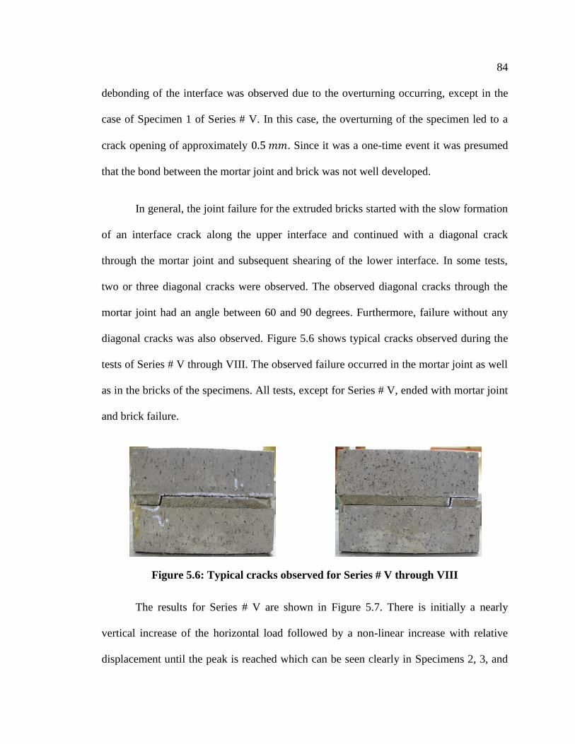
84
debonding of the interface was observed due to the overturning occurring, except in the
case of Specimen 1 of Series # V. In this case, the overturning of the specimen led to a
crack opening of approximately . Since it was a one-time event it was presumed
that the bond between the mortar joint and brick was not well developed.
In general, the joint failure for the extruded bricks started with the slow formation
of an interface crack along the upper interface and continued with a diagonal crack
through the mortar joint and subsequent shearing of the lower interface. In some tests,
two or three diagonal cracks were observed. The observed diagonal cracks through the
mortar joint had an angle between 60 and 90 degrees. Furthermore, failure without any
diagonal cracks was also observed. Figure 5.6 shows typical cracks observed during the
tests of Series # V through VIII. The observed failure occurred in the mortar joint as well
as in the bricks of the specimens. All tests, except for Series # V, ended with mortar joint
and brick failure.
Figure 5.6: Typical cracks observed for Series # V through VIII
The results for Series # V are shown in Figure 5.7. There is initially a nearly
vertical increase of the horizontal load followed by a non-linear increase with relative
displacement until the peak is reached which can be seen clearly in Specimens 2, 3, and
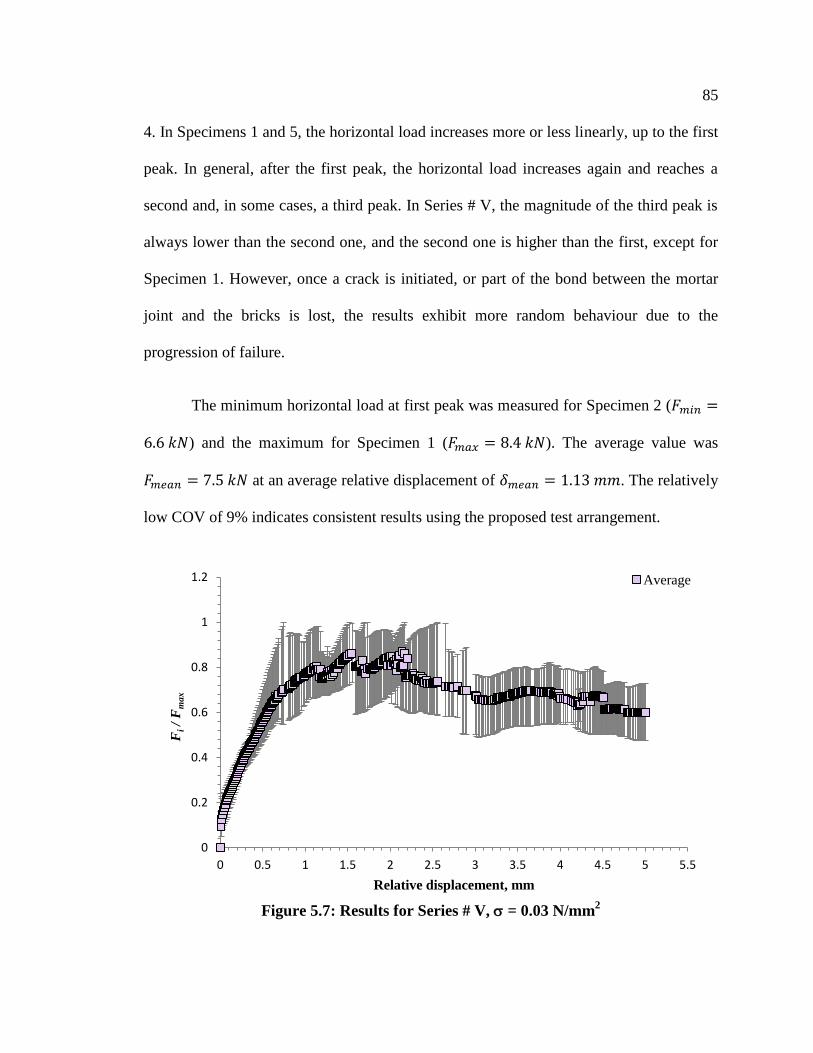
85
4. In Specimens 1 and 5, the horizontal load increases more or less linearly, up to the first
peak. In general, after the first peak, the horizontal load increases again and reaches a
second and, in some cases, a third peak. In Series # V, the magnitude of the third peak is
always lower than the second one, and the second one is higher than the first, except for
Specimen 1. However, once a crack is initiated, or part of the bond between the mortar
joint and the bricks is lost, the results exhibit more random behaviour due to the
progression of failure.
The minimum horizontal load at first peak was measured for Specimen 2 (
) and the maximum for Specimen 1 ( ). The average value was
at an average relative displacement of . The relatively
low COV of 9% indicates consistent results using the proposed test arrangement.
Figure 5.7: Results for Series # V, = 0.03 N/mm
2
0
0.2
0.4
0.6
0.8
1
1.2
0 0.5 1 1.5 2 2.5 3 3.5 4 4.5 5 5.5
Fi /
Fm
ax
Relative displacement, mm
Average
86
The results of Series # VI, as shown in Figure 5.8, also exhibit a nearly vertical
increase in the horizontal load followed by a non-linear increase until the first peak was
reached. Prior to the first peak, Specimens 1, 3, and 4 exhibited different failure
progression than Specimens 2 and 5. After the first peak, it was difficult to define the
exact point of failure. Therefore, the testing of each specimen was stopped once a relative
displacement between the upper and lower brick of approximately of was reached.
In Series # VI, failure occurred in the mortar bed joint as well as in the brick. It was
unclear which one occurred first, therefore it was assumed that the first noticeable drop in
the horizontal load was due to the failure of the mortar joint.
The minimum horizontal load at first peak was observed for Specimen 1 (
) and the maximum for Specimen 3 ( ). The average value for the
horizontal load at first peak was at an average relative displacement of
. The consistency of the load at first peak is evident by the low COV
of 10% which is also an indicator of the reproducibility using this test arrangement.
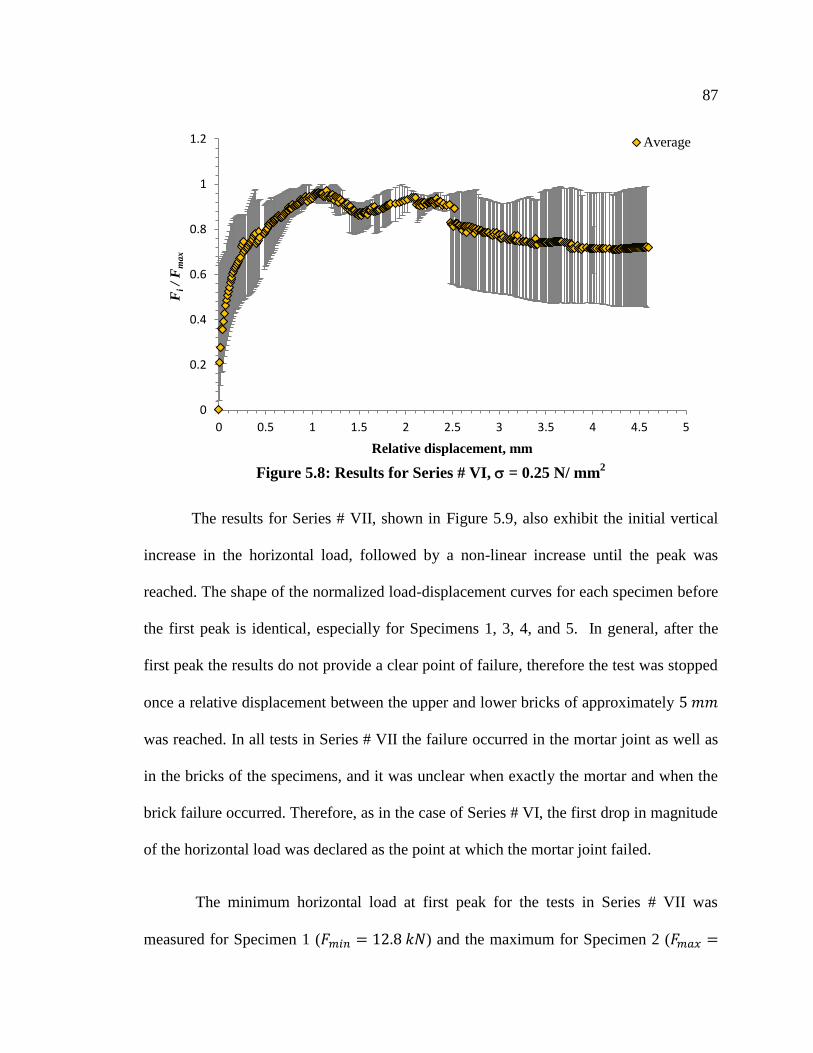
87
Figure 5.8: Results for Series # VI, = 0.25 N/ mm
2
The results for Series # VII, shown in Figure 5.9, also exhibit the initial vertical
increase in the horizontal load, followed by a non-linear increase until the peak was
reached. The shape of the normalized load-displacement curves for each specimen before
the first peak is identical, especially for Specimens 1, 3, 4, and 5. In general, after the
first peak the results do not provide a clear point of failure, therefore the test was stopped
once a relative displacement between the upper and lower bricks of approximately
was reached. In all tests in Series # VII the failure occurred in the mortar joint as well as
in the bricks of the specimens, and it was unclear when exactly the mortar and when the
brick failure occurred. Therefore, as in the case of Series # VI, the first drop in magnitude
of the horizontal load was declared as the point at which the mortar joint failed.
The minimum horizontal load at first peak for the tests in Series # VII was
measured for Specimen 1 ( ) and the maximum for Specimen 2 (
0
0.2
0.4
0.6
0.8
1
1.2
0 0.5 1 1.5 2 2.5 3 3.5 4 4.5 5
Fi /
Fm
ax
Relative displacement, mm
Average
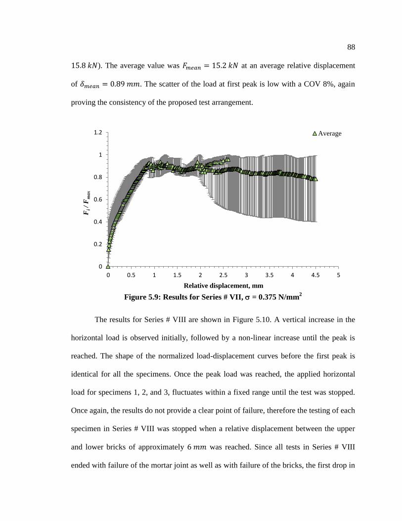
88
). The average value was at an average relative displacement
of . The scatter of the load at first peak is low with a COV 8%, again
proving the consistency of the proposed test arrangement.
Figure 5.9: Results for Series # VII, = 0.375 N/mm
2
The results for Series # VIII are shown in Figure 5.10. A vertical increase in the
horizontal load is observed initially, followed by a non-linear increase until the peak is
reached. The shape of the normalized load-displacement curves before the first peak is
identical for all the specimens. Once the peak load was reached, the applied horizontal
load for specimens 1, 2, and 3, fluctuates within a fixed range until the test was stopped.
Once again, the results do not provide a clear point of failure, therefore the testing of each
specimen in Series # VIII was stopped when a relative displacement between the upper
and lower bricks of approximately was reached. Since all tests in Series # VIII
ended with failure of the mortar joint as well as with failure of the bricks, the first drop in
0
0.2
0.4
0.6
0.8
1
1.2
0 0.5 1 1.5 2 2.5 3 3.5 4 4.5 5
Fi /
Fm
ax
Relative displacement, mm
Average
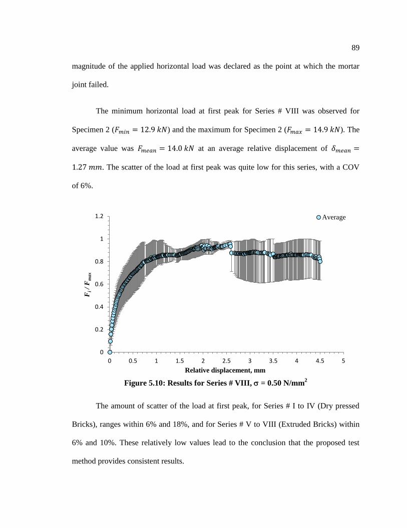
89
magnitude of the applied horizontal load was declared as the point at which the mortar
joint failed.
The minimum horizontal load at first peak for Series # VIII was observed for
Specimen 2 ( ) and the maximum for Specimen 2 ( ). The
average value was at an average relative displacement of
. The scatter of the load at first peak was quite low for this series, with a COV
of 6%.
Figure 5.10: Results for Series # VIII, = 0.50 N/mm
2
The amount of scatter of the load at first peak, for Series # I to IV (Dry pressed
Bricks), ranges within 6% and 18%, and for Series # V to VIII (Extruded Bricks) within
6% and 10%. These relatively low values lead to the conclusion that the proposed test
method provides consistent results.
0
0.2
0.4
0.6
0.8
1
1.2
0 0.5 1 1.5 2 2.5 3 3.5 4 4.5 5
Fi /
Fm
ax
Relative displacement, mm
Average
90
5.2.2 Discussion
The rotation observed in all specimens is the result of the eccentrically applied
horizontal load. Figure 5.11 illustrates the difference between the line of action of the
externally applied forces and the internal reaction forces which cause overturning of the
specimens. The overturning of the specimens leads to areas of stress concentrations at the
right (directly above the mortar joint in the lower area of the upper brick) and left
(directly beneath the mortar joint in the upper area of the lower brick) ends of the
specimens. Drawing an imaginary line between those two areas indicates the flow of the
applied load between the action and reaction points, and thereby the existence of tensile
force. Therefore, even though no cracking or debonding of the bond along the interface
due to the overturning of the specimens was observed, it is presumed that the initiation of
the crack was a result of the specimens being subjected to combined tension and shear at
this stage of the testing. However, due to the observed failure mode in the mortar joint, it
is presumed that once the crack was initiated, the crack propagation process was
governed by the applied shear force. Furthermore, the overturning of the specimens leads
to an increase in the pre-applied vertical load which was intended to counter the induced
moment due to the applied horizontal load. Obviously, the increase of the pre-applied
vertical load is not large enough to avoid the overturning of the specimens and therefore
an improvement to the test arrangement is necessary.

91
Figure 5.11: Moment and stress concentration due to eccentrically applied load
During the testing, a second peak in the applied horizontal load with a larger
magnitude than the first one was often observed. The second peak in the horizontal load,
could be due to the mechanical anchorage provided by the amount of mortar that flowed
into the cores of the bricks during the manufacturing of the specimens. The bricks were
connected to each other with a shape of mortar as shown in Figure 5.12, rather than a
uniform mortar layer with a thickness of .
Brick
+
Mortar
+
Brick
=
Specimen
Figure 5.12: Test specimens
Shrinkage of the mortar may have caused a small gap between the interior surface
of the brick core and the mortar cylinder, however, once the bond between the mortar
joint and brick at the interface is lost, and a small displacement along the joint occurs, the
mechanical anchorage of these mortar cylinders takes effect, and it is obvious that
additional horizontal load will be required to shear through these three cylinders of
mortar. Therefore, depending on diameter, height, density, and rigidity of these three
FR
FR
FR
MM
M
Stress
concetration
Stress
concetration
Stress
concentration
Stress
concentration
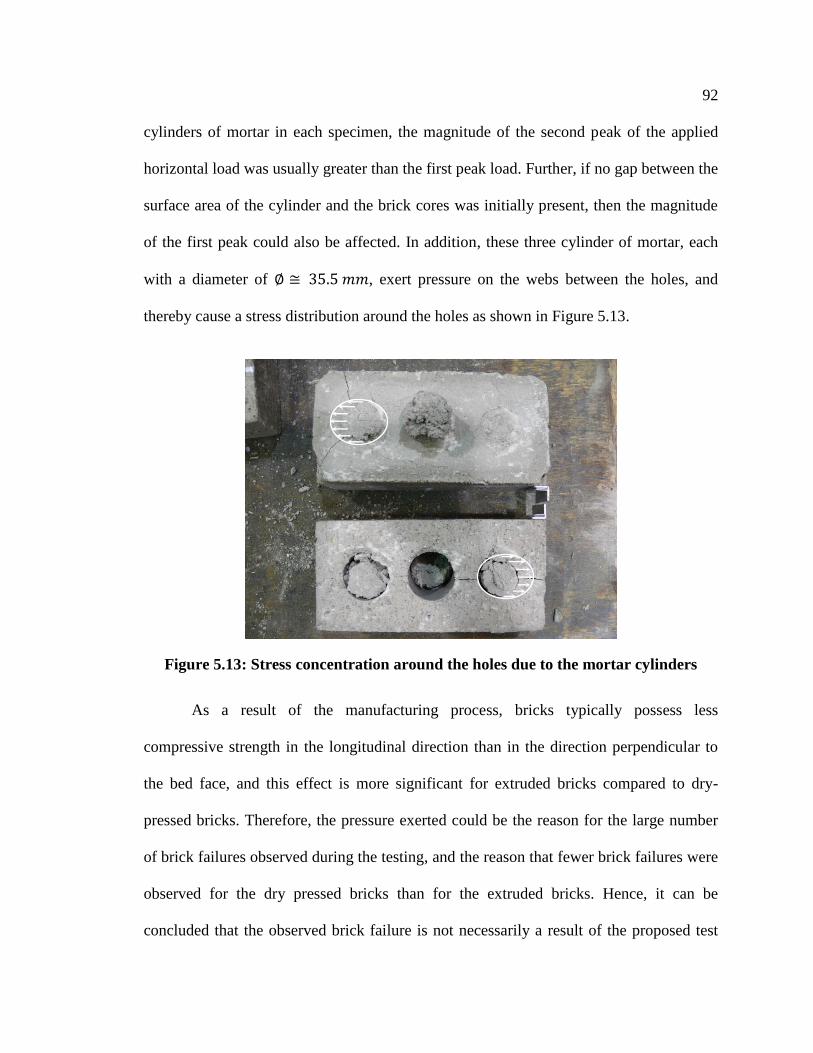
92
cylinders of mortar in each specimen, the magnitude of the second peak of the applied
horizontal load was usually greater than the first peak load. Further, if no gap between the
surface area of the cylinder and the brick cores was initially present, then the magnitude
of the first peak could also be affected. In addition, these three cylinder of mortar, each
with a diameter of , exert pressure on the webs between the holes, and
thereby cause a stress distribution around the holes as shown in Figure 5.13.
Figure 5.13: Stress concentration around the holes due to the mortar cylinders
As a result of the manufacturing process, bricks typically possess less
compressive strength in the longitudinal direction than in the direction perpendicular to
the bed face, and this effect is more significant for extruded bricks compared to dry-
pressed bricks. Therefore, the pressure exerted could be the reason for the large number
of brick failures observed during the testing, and the reason that fewer brick failures were
observed for the dry pressed bricks than for the extruded bricks. Hence, it can be
concluded that the observed brick failure is not necessarily a result of the proposed test
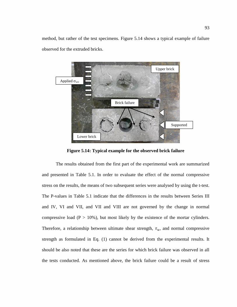
93
method, but rather of the test specimens. Figure 5.14 shows a typical example of failure
observed for the extruded bricks.
Figure 5.14: Typical example for the observed brick failure
The results obtained from the first part of the experimental work are summarized
and presented in Table 5.1. In order to evaluate the effect of the normal compressive
stress on the results, the means of two subsequent series were analysed by using the t-test.
The P-values in Table 5.1 indicate that the differences in the results between Series III
and IV, VI and VII, and VII and VIII are not governed by the change in normal
compressive load (P > 10%), but most likely by the existence of the mortar cylinders.
Therefore, a relationship between ultimate shear strength, , and normal compressive
strength as formulated in Eq. (1) cannot be derived from the experimental results. It
should be also noted that these are the series for which brick failure was observed in all
the tests conducted. As mentioned above, the brick failure could be a result of stress
Lower brick
Upper brick
Supported
Applied i(t)
Brick failure
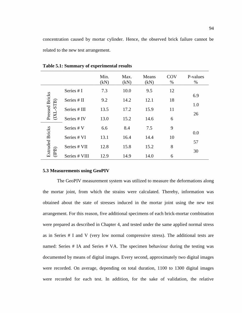
94
concentration caused by mortar cylinder. Hence, the observed brick failure cannot be
related to the new test arrangement.
Table 5.1: Summary of experimental results
Min.
(kN)
Max.
(kN)
Means
(kN)
COV
%
P-values
%
Pre
ssed
Bri
cks
(IX
L-S
TB
)
Series # I 7.3 10.0 9.5 12 6.9
1.0
26
Series # II 9.2 14.2 12.1 18
Series # III 13.5 17.2 15.9 11
Series # IV 13.0 15.2 14.6 6
Extr
uded
Bri
cks
(IP
B)
Series # V 6.6 8.4 7.5 9 0.0
57
30
Series # VI 13.1 16.4 14.4 10
Series # VII 12.8 15.8 15.2 8
Series # VIII 12.9 14.9 14.0 6
5.3 Measurements using GeoPIV
The GeoPIV measurement system was utilized to measure the deformations along
the mortar joint, from which the strains were calculated. Thereby, information was
obtained about the state of stresses induced in the mortar joint using the new test
arrangement. For this reason, five additional specimens of each brick-mortar combination
were prepared as described in Chapter 4, and tested under the same applied normal stress
as in Series # I and V (very low normal compressive stress). The additional tests are
named: Series # IA and Series # VA. The specimen behaviour during the testing was
documented by means of digital images. Every second, approximately two digital images
were recorded. On average, depending on total duration, 1100 to 1300 digital images
were recorded for each test. In addition, for the sake of validation, the relative
95
displacement between the upper and lower bricks was also recorded every second using
LSCs.
5.3.1 Methodology of Analysis
The recorded digital images were analysed using a MATLAB module described
in Chapter 4. Before applying the MATLAB module, a factor for converting coordinates
from image-space to object-space was determined. To obtain the factor, the difference in
pixels between two points was divided by the actual distance between the two points. For
each specimen, this calculation was carried out for six pairs of points selected along the
outer edges of the specimens, and an average factor of was obtained.
The accuracy of this factor is evident by the very low COV of 0.35%.
In the analysis, 10 patches were selected along the length of the mortar joint with
the aim to obtain the shear strain level in the mortar joint. In addition, 10 further patches
were selected close to the mortar-brick interface with the intent to determine the shear
strain distribution along the interfaces, as shown in Figure 5.15. In the figure, the small
squares are the patches selected.
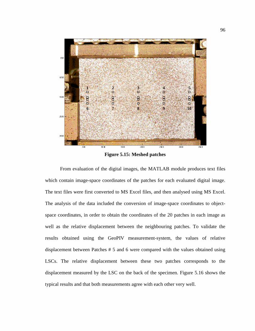
96
Figure 5.15: Meshed patches
From evaluation of the digital images, the MATLAB module produces text files
which contain image-space coordinates of the patches for each evaluated digital image.
The text files were first converted to MS Excel files, and then analysed using MS Excel.
The analysis of the data included the conversion of image-space coordinates to object-
space coordinates, in order to obtain the coordinates of the 20 patches in each image as
well as the relative displacement between the neighbouring patches. To validate the
results obtained using the GeoPIV measurement-system, the values of relative
displacement between Patches # 5 and 6 were compared with the values obtained using
LSCs. The relative displacement between these two patches corresponds to the
displacement measured by the LSC on the back of the specimen. Figure 5.16 shows the
typical results and that both measurements agree with each other very well.
1 2 3 4 5
6 7 8 9 10
0
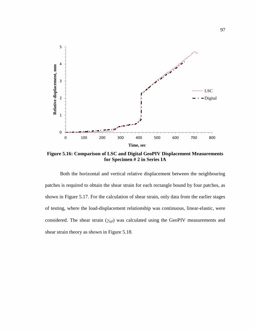
97
Figure 5.16: Comparison of LSC and Digital GeoPIV Displacement Measurements
for Specimen # 2 in Series IA
Both the horizontal and vertical relative displacement between the neighbouring
patches is required to obtain the shear strain for each rectangle bound by four patches, as
shown in Figure 5.17. For the calculation of shear strain, only data from the earlier stages
of testing, where the load-displacement relationship was continuous, linear-elastic, were
considered. The shear strain () was calculated using the GeoPIV measurements and
shear strain theory as shown in Figure 5.18.
0
1
2
3
4
5
0 100 200 300 400 500 600 700 800
Rel
ati
ve
dis
pla
cem
ent,
mm
Time, sec
LSC
Digital
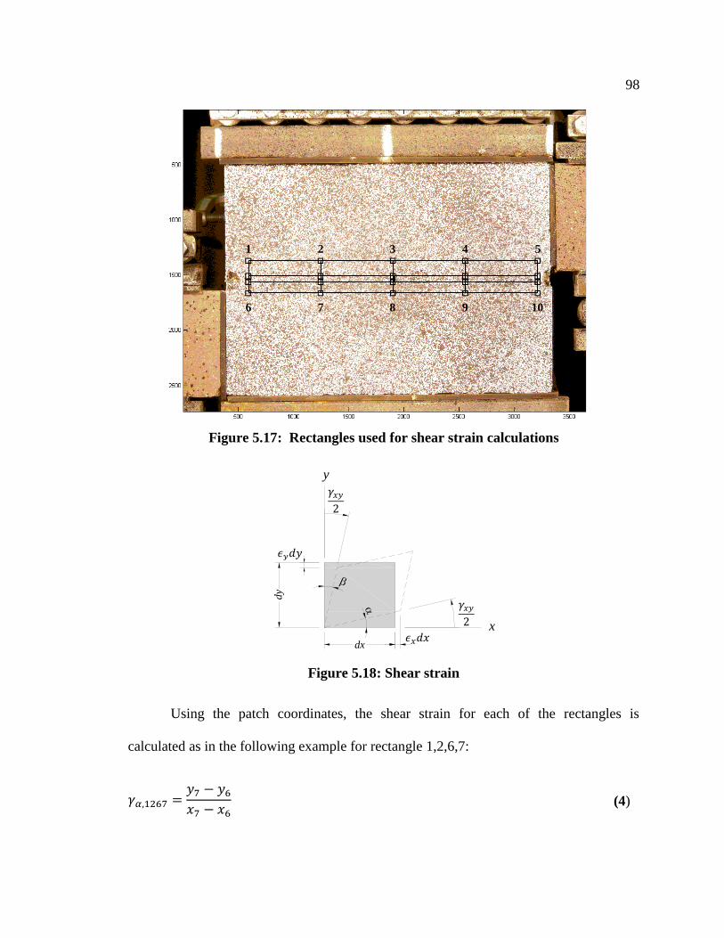
98
Figure 5.17: Rectangles used for shear strain calculations
Figure 5.18: Shear strain
Using the patch coordinates, the shear strain for each of the rectangles is
calculated as in the following example for rectangle 1,2,6,7:
(4)
dy
dx
x
y
1 2 3 4 5
6 7 8 9 10
0
99
(5)
(6)
5.3.2 Results & Discussion
Initially, the shear strain, , in the mortar joint was calculated using equations
(4) through (6) from the relative displacement of the 10 patches in the mortar joint
(unnumbered patches in Figure 5.17). The mean results are listed with the corresponding
time frame, COV, and load in Table 5.2. Assuming a constant shear modulus, the shear
stress along the mortar joint can be calculated from the shear strain using Eq. (7) and
Eq.(8), where is the shear stress along the mortar joint at time , is the
calculated shear strain at time , and G, and are the Shear modulus, Young’s modulus
and the Poisson’s ratio of the mortar, respectively.
(7)
( ) (8)
Some important observations can be made from the results in Table 5.2. First of
all, considering the magnitude of the corresponding loads, one would expect average
shear stresses in the order of to . However, the calculated results for
shear stress, listed in Table 5.2, are much higher, which is unreasonable. The error
in calculating the shear stresses could result from a variety of sources. First, the
properties of the mortar given in Table 3.1, are selected from the literature, and therefore
differ from the actual properties of the mortar used in this research program. Secondly,
100
Eq. (8) is based on the assumption that the material is isotropic, homogeneous and
behaves in a linear-elastic manner. Although masonry is often assumed to be an isotropic
and homogenous material, and this assumption may lead to reasonable results at the
meso- and macro-level, at the micro-level, where the units and joints are considered
separately, this assumption is questionable. The very nature of the constituent materials
and the mixing and placing of the mortar make it nearly impossible to guarantee
homogeneity of the mortar joint. In addition, Eq. (7) is derived for materials subjected to
pure shear. This is not the case for the test method used in this research because the
eccentrically applied load also produces a bending moment. Therefore, more research is
necessary to obtain the properties of the mortar, and the knowledge obtained can then be
used to determine the exact state of stress along the mortar joint.
Another important observation from Table 5.2 is that the shear strain values are
very scattered indicating a non-uniform distribution of the shear strain in the mortar joint.
The high variation in the strain could also result from a variety of sources including the
mortar properties and the graphical resolution. With the 10 Megapixel camera utilized, a
movement of one pixel represents a displacement of in reality. The effect of
graphical resolution becomes particularly noticeable in the case of very small relative
displacements (less than one pixel), and results in a higher amount of scatter as seen at
the earlier stages of testing in Table 5.2. This is also the most likely explanation for the
extremely high variation in the normal strain (also reported in Table 5.2). In addition,
since the mortar is a granular material, the irregularity in the results of normal and shear
strain in the middle of the joint may also be due to dilation that occurs when the fractured
101
surfaces slide past each other during the testing procedure. As noted, a movement of one
pixel represents a displacement of only in reality. Hence, a very small
displacement, either positive or negative, in the vertical direction will contribute to the
irregularity of the results. Therefore, a digital camera with a graphical resolution of at
least 15 Megapixels is recommended.
Since the results within the mortar joint were likely affected significantly by the
graphical resolution, a larger area of analysis was chosen to try to minimize this effect.
Therefore, additional patches (numbered 1 – 10 in Figure 5.17) were selected at the
mortar-brick interface to obtain the strains over the entire joint.
In Table 5.3, the mean results for shear strain ( ) calculated from the relative
displacement of the 10 patches at the mortar-brick interfaces are listed with the
corresponding time frame, COV, and load. The low amount of scatter of the shear strain
values leads to the conclusion that the distribution of the shear strain, and consequently
the shear stress, along the joint is uniform. As discussed above, the shear modulus, G, for
the mortar cannot be determined, thus, the average shear stress in the joint was calculated
using Eq. (9):
(9)
where is the average shear stress along the joint at time ,
is the measured
applied horizontal load at time , and is the gross cross-sectional area at the interface.
The results for shear stress obtained using Eq. (9) are also listed in Table 5.3. Unlike the
102
shear strain, the values of the normal strain, y, (i.e. normal to the mortar joint) still
indicate a non-uniform distribution as evident by the high value of COV. However, as
mentioned above, the high COVs for the normal strains are most likely due to the very
small displacements, either positive or negative, in the vertical direction and insufficient
graphical resolution provided by the 10 Megapixel camera. Scatter in the normal strains
may also be related to the bending moment that is induced by the eccentrically applied
horizontal load (overturning did occur as evidenced by the uplift).
The results obtained from the FEM analysis in Chapter 3 indicated that the
proposed test arrangement produces a more uniform stress distribution than the triplet test
and the results are as good as, if not better than, the Hofmann & Stöckl test. However, in
order to compare the state of strain/stress for the triplet and Hofmann & Stöckl tests,
experiments using the GeoPIV measurement system would be necessary.
103
Table 5.2: Mean values for four rectangles selected within the mortar joint
Time
(sec) COV
(%)
Load
(N)
i, joint(N/mm
2)
y COV
(%)
Dry Pressed Bricks
Sp
ecim
en I
A-1
117 0.0005 105 2000 1.8 0.001 128
155 0.0013 49 3000 4.7 0.0006 311
192 0.0015 64 4000 5.4 0.0008 226
229 0.0018 42 5000 6.5 0.0009 233
Spec
imen
IA
-2 242 0.0014 139 4774 5.0 0.0005 158
257 0.0017 137 5518 6.0 0.0006 197
273 0.0023 170 6263 8.0 0.0009 203
288 0.0030 188 7007 10.8 0.0018 207
Spec
imen
IA
-3 151 0.0005 90 3125 1.8 0.0001 303
168 0.0008 89 3750 2.9 0.0002 392
185 0.0015 127 4375 5.4 0.0007 211
202 0.0031 143 5000 11.2 0.0010 189
Spec
imen
IA
-4 203 0.0008 45 3375 2.9 0.0002 125
228 0.0005 67 4250 1.8 0.0001 162
252 0.0007 70 5125 2.5 0.0001 170
277 0.0006 81 6000 2.2 0.0002 112
Sp
ecim
en I
A-5
144 0.0007 113 3771 2.5 0.0012 125
162 0.0014 91 4526 5.0 0.0012 160
180 0.0006 72 5280 2.2 0.0014 137
198 0.0018 93 6034 6.5 0.0015 167
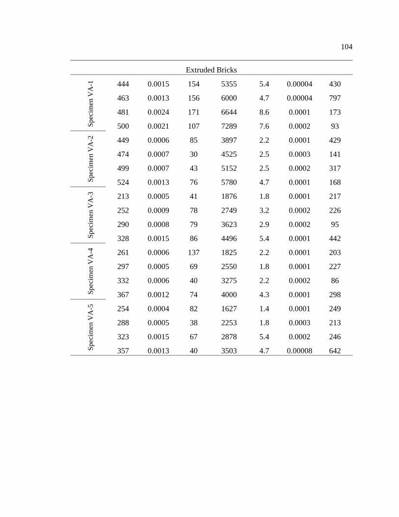
104
Extruded Bricks
Sp
ecim
en V
A-1
444 0.0015 154 5355 5.4 0.00004 430
463 0.0013 156 6000 4.7 0.00004 797
481 0.0024 171 6644 8.6 0.0001 173
500 0.0021 107 7289 7.6 0.0002 93
Sp
ecim
en V
A-2
449 0.0006 85 3897 2.2 0.0001 429
474 0.0007 30 4525 2.5 0.0003 141
499 0.0007 43 5152 2.5 0.0002 317
524 0.0013 76 5780 4.7 0.0001 168
Spec
imen
VA
-3
213 0.0005 41 1876 1.8 0.0001 217
252 0.0009 78 2749 3.2 0.0002 226
290 0.0008 79 3623 2.9 0.0002 95
328 0.0015 86 4496 5.4 0.0001 442
Spec
imen
VA
-4
261 0.0006 137 1825 2.2 0.0001 203
297 0.0005 69 2550 1.8 0.0001 227
332 0.0006 40 3275 2.2 0.0002 86
367 0.0012 74 4000 4.3 0.0001 298
Spec
imen
VA
-5
254 0.0004 82 1627 1.4 0.0001 249
288 0.0005 38 2253 1.8 0.0003 213
323 0.0015 67 2878 5.4 0.0002 246
357 0.0013 40 3503 4.7 0.00008 642
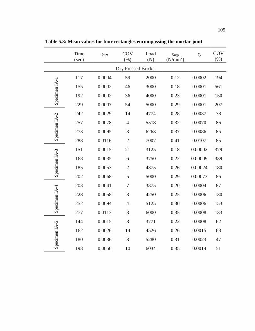
105
Table 5.3: Mean values for four rectangles encompassing the mortar joint
Time
(sec) COV
(%)
Load
(N)
avgi
(N/mm2)
y COV
(%)
Dry Pressed Bricks
Sp
ecim
en I
A-1
117 0.0004 59 2000 0.12 0.0002 194
155 0.0002 46 3000 0.18 0.0001 561
192 0.0002 36 4000 0.23 0.0001 150
229 0.0007 54 5000 0.29 0.0001 207
Spec
imen
IA
-2 242 0.0029 14 4774 0.28 0.0037 78
257 0.0078 4 5518 0.32 0.0070 86
273 0.0095 3 6263 0.37 0.0086 85
288 0.0116 2 7007 0.41 0.0107 85
Spec
imen
IA
-3 151 0.0015 21 3125 0.18 0.00002 379
168 0.0035 6 3750 0.22 0.00009 339
185 0.0053 2 4375 0.26 0.00024 180
202 0.0068 5 5000 0.29 0.00073 86
Spec
imen
IA
-4 203 0.0041 7 3375 0.20 0.0004 87
228 0.0058 3 4250 0.25 0.0006 130
252 0.0094 4 5125 0.30 0.0006 153
277 0.0113 3 6000 0.35 0.0008 133
Sp
ecim
en I
A-5
144 0.0015 8 3771 0.22 0.0008 62
162 0.0026 14 4526 0.26 0.0015 68
180 0.0036 3 5280 0.31 0.0023 47
198 0.0050 10 6034 0.35 0.0014 51
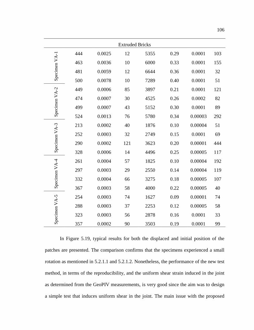
106
Extruded Bricks
Sp
ecim
en V
A-1
444 0.0025 12 5355 0.29 0.0001 103
463 0.0036 10 6000 0.33 0.0001 155
481 0.0059 12 6644 0.36 0.0001 32
500 0.0078 10 7289 0.40 0.0001 51
Sp
ecim
en V
A-2
449 0.0006 85 3897 0.21 0.0001 121
474 0.0007 30 4525 0.26 0.0002 82
499 0.0007 43 5152 0.30 0.0001 89
524 0.0013 76 5780 0.34 0.00003 292
Spec
imen
VA
-3
213 0.0002 40 1876 0.10 0.00004 51
252 0.0003 32 2749 0.15 0.0001 69
290 0.0002 121 3623 0.20 0.00001 444
328 0.0006 14 4496 0.25 0.00005 117
Spec
imen
VA
-4
261 0.0004 57 1825 0.10 0.00004 192
297 0.0003 29 2550 0.14 0.00004 119
332 0.0004 66 3275 0.18 0.00005 107
367 0.0003 58 4000 0.22 0.00005 40
Spec
imen
VA
-5
254 0.0003 74 1627 0.09 0.00001 74
288 0.0003 37 2253 0.12 0.00005 58
323 0.0003 56 2878 0.16 0.0001 33
357 0.0002 90 3503 0.19 0.0001 99
In Figure 5.19, typical results for both the displaced and initial position of the
patches are presented. The comparison confirms that the specimens experienced a small
rotation as mentioned in 5.2.1.1 and 5.2.1.2. Nonetheless, the performance of the new test
method, in terms of the reproducibility, and the uniform shear strain induced in the joint
as determined from the GeoPIV measurements, is very good since the aim was to design
a simple test that induces uniform shear in the joint. The main issue with the proposed
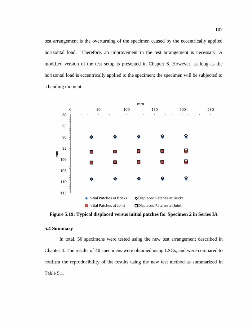
107
test arrangement is the overturning of the specimen caused by the eccentrically applied
horizontal load. Therefore, an improvement in the test arrangement is necessary. A
modified version of the test setup is presented in Chapter 6. However, as long as the
horizontal load is eccentrically applied to the specimen; the specimen will be subjected to
a bending moment.
Figure 5.19: Typical displaced versus initial patches for Specimen 2 in Series IA
5.4 Summary
In total, 50 specimens were tested using the new test arrangement described in
Chapter 4. The results of 40 specimens were obtained using LSCs, and were compared to
confirm the reproducibility of the results using the new test method as summarized in
Table 5.1.
80
85
90
95
100
105
110
115
0 50 100 150 200 250
mm
mm
Initial Patches at Bricks Displaced Patches at Bricks
Initial Patches at Joint Displaced Patches at Joint
108
Ten further tests were conducted using a digital imaging measurement technique
which made it possible to calculate strains in the specimens. The digital images were
evaluated using a MATLAB-module named GeoPIV. The results presented in Table 5.3
show that the new test method produces uniform shear strain along the joint.
The experimental work as well as the data analysis indicates that the main issue
with the new test method is the small overturning of the specimens due to the
eccentrically applied horizontal load. Therefore, a modification of the test method is
necessary to minimize the overturning as much as possible.
109
CHAPTER 6: CONCLUSIONS & RECOMMENDATIONS
6.1 Summary
In a structure made of masonry, lateral loads, caused by wind or earthquake, are
resisted by masonry shear walls. The shear strength of a masonry wall depends on many
factors including the strength of units and the mortar bed joints. Therefore, over the last
few decades, several test arrangements were devised and utilized by researchers to
examine the shear strength of a mortar bed joint. The numerical analysis presented in this
thesis shows that the Hofmann & Stöckl test produces nearly uniform normal and shear
stresses along the bed joint, however it requires very complex equipment. On the other
hand, the triplet test is simpler to perform, but the numerical analysis showed that it does
not produce uniformly distributed stress.
The new test method described in this thesis was devised to combine the
advantages of the Hofmann & Stöckl and the triplet tests. In the test arrangement
designed, the couplet can be subjected to a horizontal load or to a combination of
horizontal and vertical loads. The proposed test method was initially compared with the
triplet and Hofmann & Stöckl tests using a two-dimensional finite element model in the
commercial software package SAP2000. In addition to the FEM evaluation, an
experimental program was conducted. Couplets constructed of two types of clay bricks
(dry-pressed and extruded) and one type of mortar (Type S) were tested to evaluate the
reproducibility of the results using the new test method. In total, 50 specimens, 25 for
each brick type, were tested at four different levels of normal pre-compressive stress. The
relative displacements between the upper and lower bricks of the specimen were
110
measured with linear strain converters (LSCs), and also a measurement system based on
Particle Image Velocimetry (GeoPIV).
6.2 Conclusions
The conclusions below are derived from the results of the numerical evaluation
and the results of the experimental program presented in Chapters 3 and 5, respectively.
6.2.1 Finite element model
The results obtained from Case Study 1 prove that the new test method is capable
of producing desirable results for nearly uniform shear stress in a mortar joint, and that no
tensile stress is induced in the bed joint. Compared to the triplet test, the resulting
distributions of normal and shear stresses in the new test method are more uniform, and
are based only on one mortar joint, rather than two as in the triplet test, which only
provides results for the weakest one. Further, unlike the case of the triplet test, no tensile
stress is induced in the bed joint. Compared to the Hofmann & Stöckl test, the
distribution of shear stress in the proposed test method is similar.
Results obtained from Case Study 2 indicate that the magnitude of normal tensile
stress along the mortar joint for the Hofmann & Stöckl test is not as high as reported in
the literature.
The finite element evaluations show that the new test method can clearly be an
alternative to the Hofmann & Stöckl and triplet tests.
111
6.2.2 Experimental work
A new test arrangement was constructed using simple equipment which can be
found in any civil engineering laboratory. The new test method was used to test 50
couplets. The tests conducted were divided into eight series with varying levels of pre-
compression. The load-displacement behaviour of 40 specimens based on measurements
using Linear Strain Converters (LSCs) proves that the new test method generates
reproducible results. The peak values for load-displacement behaviour measured during
the experimental work were affected by the amount of mortar that flowed into the holes
of the bricks when the specimens were constructed and the resulting mechanical action
between these mortar cylinders and the bricks.
The remaining ten specimens were used in combination with the GeoPIV
measurement system to gain insight into the state of normal and shear stress that are
induced in the mortar bed joint using the new test method. The specimen behaviour
during the testing was documented by means of digital images and the images were
analysed using a MATLAB module to determine the relative displacement between user-
defined points. To the best of the author’s knowledge, this is the first time that the strain
or stress in the joint has been evaluated in any micro-level joint shear test. The results
obtained prove that the new test method produces uniform shear strain in the mortar joint.
Assuming a constant shear modulus, the shear stress will be as uniform as the strain.
However, for the shear stress calculation the application of Eq. (7),
, is questionable, since the assumption that masonry is an isotropic and
homogenous material cannot be guaranteed at the micro-level. In addition, Eq. (7),
112
, is derived for materials subjected to pure shear which was not the
case for the test method used in this research because the eccentrically applied load also
produces a bending moment.
The distribution of the normal strains did not show uniformity, most likely due to
the bending moment from the eccentrically applied horizontal load, and that the graphical
resolution was not sufficient to capture the extremely small normal deformations. The
irregularity of the results of normal and shear strain in the middle of the joint may also be
a result of the small order of magnitude of the values and from dilation that occurs during
the testing procedure.
6.3 Recommendations for future work
The results obtained from the experimental work and the GeoPIV measurements
indicate that the specimen is subjected to a small rotation during the test. This rotation is
a result of the eccentrically applied horizontal load, and of the compressibility of the
rubber sheets used to accommodate the unevenness of the surface of the bricks.
The rotation of the specimens is the main disadvantage of the new test method. To
overcome this limitation, the test setup should be modified as presented in Figure 6.1.
The modification consists of adding a support plate connected by four threaded rods to
the upper flange of the lower beam. This support plate will prevent the overturning of the
specimen to a large degree. The increase of pre-applied vertical load during the testing
phase can then be measured by the load cells placed between the support plate and hex-
nuts. In addition, a load plate with circular cross section is added to provide a surface for
113
the manually operated jack. Further improvement can be achieved either by removing the
rubber sheets and using an alternative material that is able to accommodate the
unevenness of the surface of the brick with high compressive resistance, e.g. plaster of
Paris. Further, it was concluded that the peak values measured during the experimental
work were affected by the amount of mortar that flowed into the holes of the bricks while
the specimens were constructed. Therefore, more studies about the effect of the mortar
cylinder on the load-displacement behaviour are necessary. In this regard, the cores
should be covered or plugged partially or completely to prevent mortar entering. A study
should be undertaken with the cores of the specimens unfilled and filled to four different
heights, namely: quarter, half, three-quarter, and full. This procedure will provide
knowledge about the effect of the mortar cylinders.
Besides the above suggested modifications and recommendations, the following
points are recommended:
1. The use of a digital camera with a graphical resolution of at least 15
megapixels is recommended. This combined with the above suggested
modification should significantly reduce the scatter of the results for
normal strain.
2. More research is needed to determine the stress distribution in the mortar
joint precisely.
3. FE analysis with a non-uniform compressive stress is recommended to
compare to the actual test results. The analysis is feasible with the
114
modified test arrangement and the magnitude of the vertical load that will
be provided by the cell loads, see Figure 6.1.
4. In order to compare the state of strain/stress for the triplet and Hofmann &
Stöckl test methods, experiments using the GeoPIV measurement system
would be necessary, and are recommended.
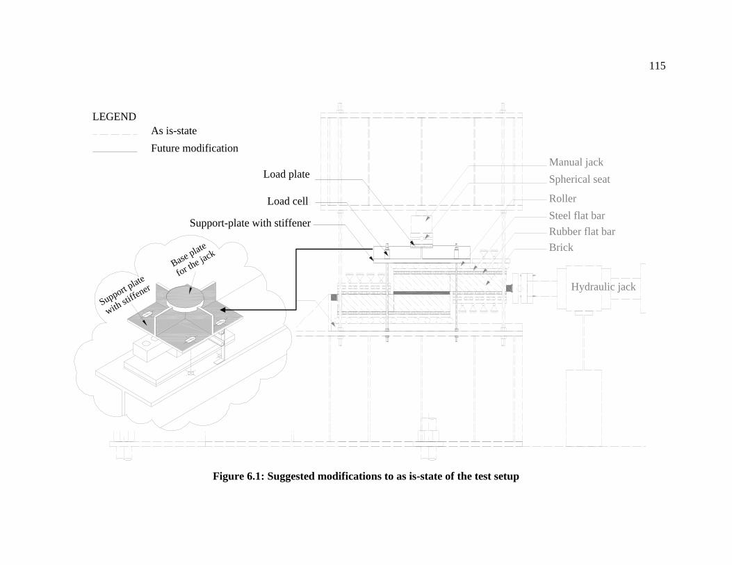
115
Figure 6.1: Suggested modifications to as is-state of the test setup
Roller
Steel flat bar
Rubber flat bar
I-Section
Hydraulic jack
Brick
Steel plate is used to have
a leveled surface.
Load plate
Load cell
Support-plate with stiffener
Spherical seat
Manual jack
LEGEND
As is-state
Future modification
Base plate
for the ja
ck
Support plate
with st
iffener
116
REFFERENCES
Adrian, R. J., 1991. Particle imaging techniques for experimental fluid mechanics. Annu.
Rev. of Fluid Mech., Volume 23, pp. 261-304.
Bisby, L. A. & Take, W. A., 2009. Strain localisations in FRP confined concrete: new
insights. s.l., s.n., pp. 1-9.
Bisby, L., Take, W. & Caspary, A., 2007. Quantifying strain variation in FRP confined
concrete using digital image analysis. Hong Kong, s.n., pp. 599-604.
Bouzeghoub, M., Jukes, P. & Riddington, J., 1995. Influence of loading arrangement on
the initial mode of failure of brick triplet shear specimens. In: Comput. Mehtod in
Structural Masonry - 3. Eds. s.l.:s.n., pp. 117-126.
CSA A179-04, C. S., 2004. Mortar and grout for unit masonry, Ontario: Canadian
Standards Association.
CSA A82-06, C. S., 2006. Fired Masonry Brick Made from Clay or Shale, Ontario:
Canadian Standard Association.
DIN EN 1052-3, I. 9., 2007. Methods of test for masonry – Part 3: Determination of
initial shear strength; German version EN 1052-3:2002 + A1:2007, Brussels:
EUROPEAN COMMITTEE FOR STANDARDIZATION.
Ghazali, M. & Riddington, J., 1986. Shear strength of brickwork. Bankok, s.n., pp. 593-
604.
Ghazali, M. & Riddington, J., 1988. Simple test method for masonry shear strength.
Proc. Institution of Civil Engineers, Part 2, Volume 85, pp. 567-574.
Hamid, A. A. & Drysdale, R. G., 1982. The shear behaviour of brickwork bed joints.
Proc. of the British Ceramic Soc., 09, Volume 30, pp. 101-109.
Hamid, A., Drysdale, R. & Heidebrecht, A. C., 1979. Shear strength of concrete masonry
joints. J. of the Structural Division, Volume 105, pp. 1227-1240.
Hansen, K. F., Nykanen, E. & Gottfredsen, F. R., 1998. Shear behaviour of bed joints at
different levels of precompression. Masonry Int., 12(2), pp. 70-78.
Hansen, K. F. & Pedersen, C. M., 2008. Torsion testing of bed joints. Int. Masonry
Society, 12(1), pp. 43-48.
Hansen, K. & Pedersen, E., 2009. Shear and torsion testing of brick-mortar joints.
Masonry Int., Volume 22, pp. 31-38.
117
Hofmann, P. & Stöckl, S., 1986. Tests on shear-bond behaviour in the bed-joints of
masonry. Masonry Int., 12, Volume 9, pp. 1-15.
Jiang, D.-H. & Xiao, X.-S., 1994. A new masonry shear test method determining masonry
shear strength. Calgary, s.n., pp. 1013-1019.
Jukes, P. & Riddington, J., 1997. A review of masonry joint shear strength test methods.
Masonry Int., Volume 11, pp. 37-43.
Khalaf, F., 1995. Simple bending test for the determination of masonry bond shear
strength. s.l., s.n.
Khalaf, F. M. & Naysmith, M. W., 1997. Shear strength of masonry bed joints. The
Masonry Society, 15(2), pp. 13-22.
Lissel, S. L., 2001. Behaviour and Design of CFRP Post-Tensioned Masonry Diaphragm
Walls, Calgary: University of Calgary.
Masia, M. J., Han, Y. & Correa, M. R. S., 2006. Torsion testing for the characterisation
of the shear behaviour of mortar joints in masonry. J. of the British Masonry Soc.,
Masnory Int., 19(2), pp. 77-88.
Masia, M. J., Petersen, R. B., Han, Y. & Correa, M. R. S., 2010. Torsion shear test for
mortar joints in masonry: experimental evaluation. J. of the Int. Masonry Soc., 09, 23(3),
pp. 91-102.
Pook, L., Stylianou, M. & Dawe, J., 1986. Experimental investigation of the influence of
compression on the shear strength of masonry joints. s.l., s.n., pp. 1053-1062.
Popal, R. & Lissel, S. L., 2010. Numerical evaluation of existing mortar joint shear tests
and a new test method. Dresden, s.n., pp. 795-802.
Riddington, J., Fong, K. & Jukes, P., 1997. Numerical study of failure initiation in
different joint shear test. Masonry Int., Volume 11, pp. 44-50.
Riddington, J. & Jukes, P., 1994. A masonry joint shear strength test method. s.l., s.n., pp.
267-274.
Riddington, J. R., Gambo, A. H. & Edgell, G. J., 1991. An assessment of the influence of
unit aspect ratio on bond shear srtength values given by the proposed CEN triplet test.
Berlin, s.n., pp. 1321-1328.
Riddington, J. R. & Ghazali, M. Z., 1987. Shear strength of masonry joints at high
normal stress levels. Kuala Lumpur, s.n., pp. 1-11.
Riddington, J. R. & Ghazali, M. Z., 1990. Hypothesis for shear failure in masonry joints.
Proc. Institution of Civil Engineers, Part 2, 03, Volume 89, pp. 89-102.
118
Samarasinghe, W. & Lawrence, S., 1994. Behaviour of masonry under combined torsion
and compression. Calgary, s.n., pp. 1057-1066.
Stöckl, S. & Hofmann, J., 1990. A Comparative finite element evaluation of mortar joint
shear tests. Masonry Int., Volume 3, pp. 101-104.
Sutcliffe, D. J., Yu, H. S. & Page, A. W., 2001. Lower bound limit analysis of
unreinforced masonry shear walls. Comput. and Structures, pp. 1295 - 1312.
van der Pluijm, R., 1992. Material properties of masonry and its components under
tension and shear. Saskatoon, s.n., pp. 675-686.
van der Pluijm, R., 1993. Shear behaviour of bed joints. Philadelphia, s.n., pp. 125-136.
van Vliet, i. M., 2004. Shear tests on masonry panels; Literature survey and proposal for
experiments, s.l.: s.n.
Vermeltfoort, A. T., 2010. Variation in shear properties of masonry. Dresden, Int.
Masonry Society.
White, D. & Take, W., 2002. GeoPIV: Paritcale Image Velocimety (PIV) software for
use in geotechnical testing, s.l.: Cambridge University Engineering Departement.
White, D., Take, W. & Bolton, M., 2001a. Measuring soil deformation in geotechnical
models using digital images and PIV analysis. Tucson, Arizona, Balkema, Rotterdam, pp.
997-1002.
White, D., Take, W., Bolton, M. & Munachen, S., 2001b. A deformation measurement
sustem for geotechnical testing based on digitla imaging, close-range photogrammetry,
and PIV image analysis. Instanbul, Turkey, Balkema, Rotterdam, pp. 539-542.

119
APPENDIX A: RAW DATA
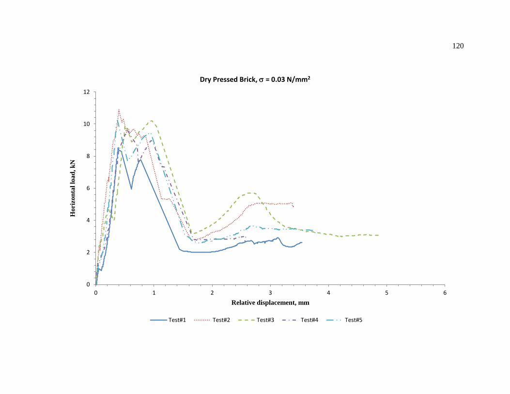
120
0
2
4
6
8
10
12
0 1 2 3 4 5 6
Hori
zon
tal
load
, k
N
Relative displacement, mm
Dry Pressed Brick, = 0.03 N/mm2
Test#1 Test#2 Test#3 Test#4 Test#5
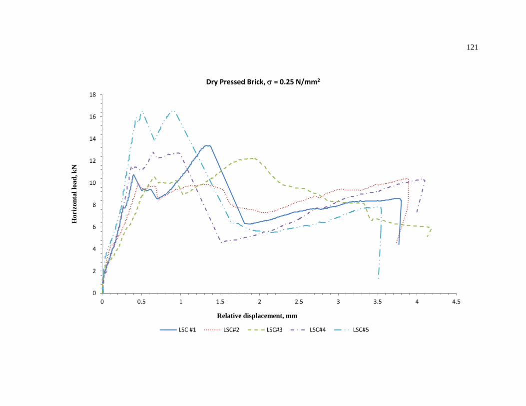
121
0
2
4
6
8
10
12
14
16
18
0 0.5 1 1.5 2 2.5 3 3.5 4 4.5
Hori
zon
tal
load
, k
N
Relative displacement, mm
Dry Pressed Brick, = 0.25 N/mm2
LSC #1 LSC#2 LSC#3 LSC#4 LSC#5
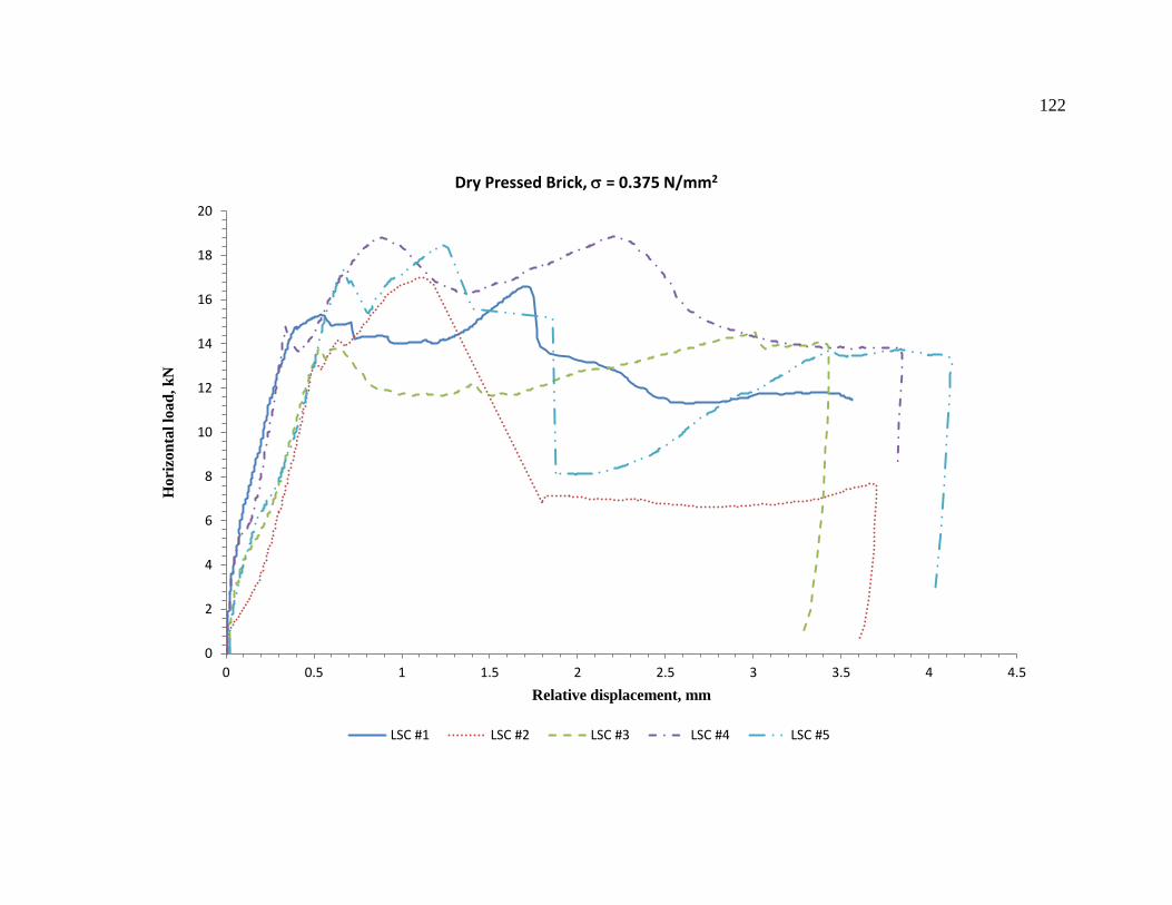
122
0
2
4
6
8
10
12
14
16
18
20
0 0.5 1 1.5 2 2.5 3 3.5 4 4.5
Hori
zon
tal
load
, k
N
Relative displacement, mm
Dry Pressed Brick, = 0.375 N/mm2
LSC #1 LSC #2 LSC #3 LSC #4 LSC #5
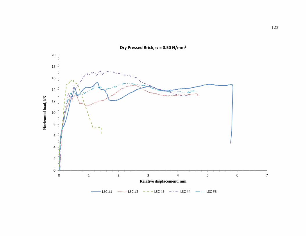
123
0
2
4
6
8
10
12
14
16
18
20
0 1 2 3 4 5 6 7
Hori
zon
tal
load
, k
N
Relative displacement, mm
Dry Pressed Brick, = 0.50 N/mm2
LSC #1 LSC #2 LSC #3 LSC #4 LSC #5
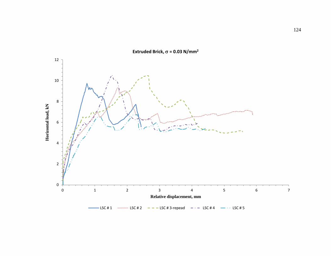
124
0
2
4
6
8
10
12
0 1 2 3 4 5 6 7
Hori
zon
tal
load
, k
N
Relative displacement, mm
Extruded Brick, = 0.03 N/mm2
LSC # 1 LSC # 2 LSC # 3-repead LSC # 4 LSC # 5
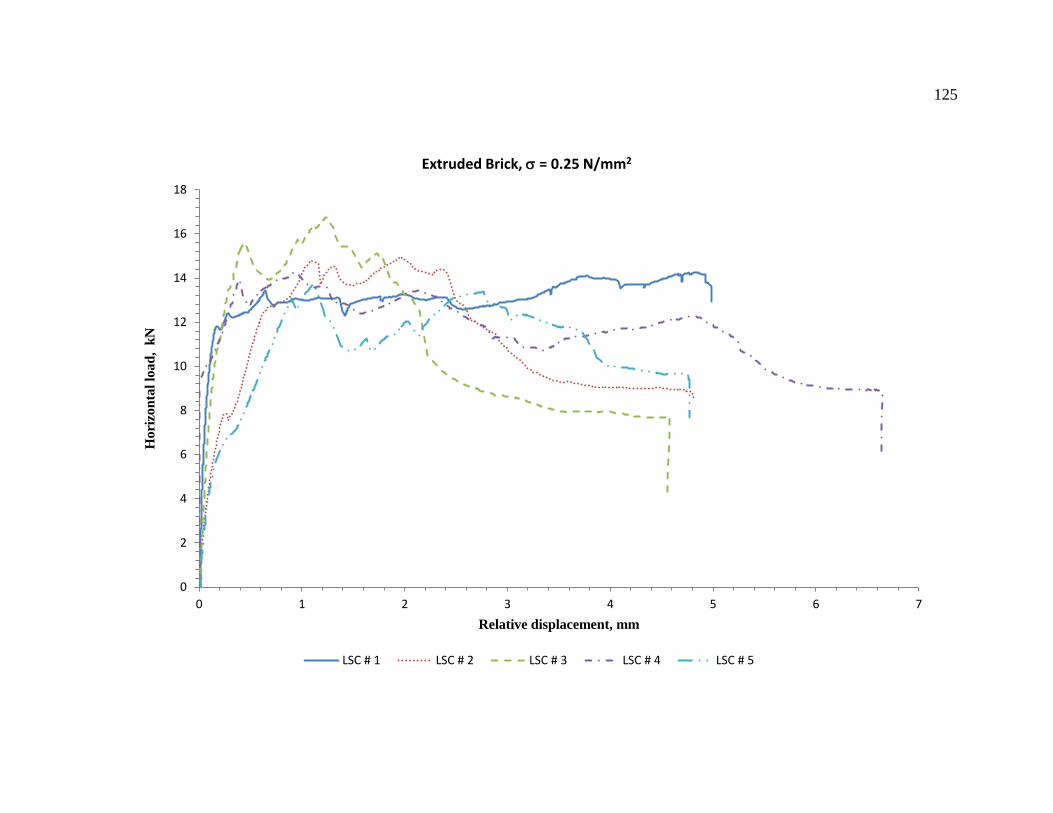
125
0
2
4
6
8
10
12
14
16
18
0 1 2 3 4 5 6 7
Hori
zon
tal
load
, k
N
Relative displacement, mm
Extruded Brick, = 0.25 N/mm2
LSC # 1 LSC # 2 LSC # 3 LSC # 4 LSC # 5
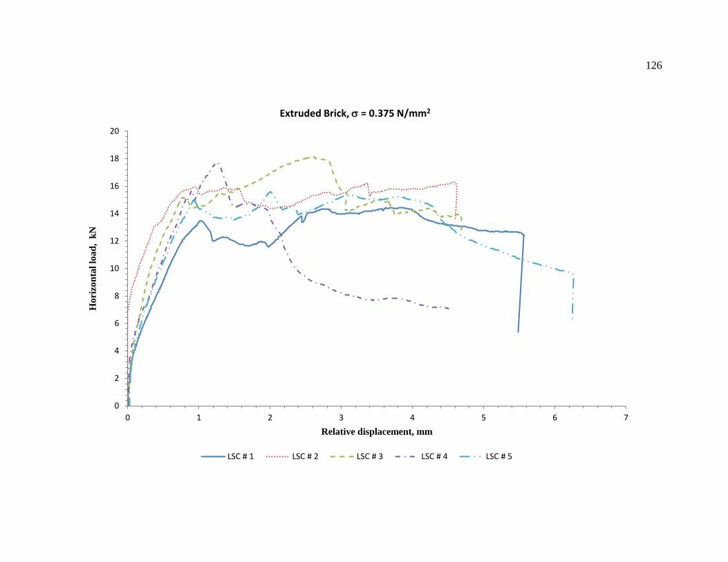
126
0
2
4
6
8
10
12
14
16
18
20
0 1 2 3 4 5 6 7
Hori
zon
tal
load
, k
N
Relative displacement, mm
Extruded Brick, = 0.375 N/mm2
LSC # 1 LSC # 2 LSC # 3 LSC # 4 LSC # 5
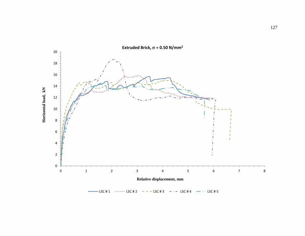
127
0
2
4
6
8
10
12
14
16
18
20
0 1 2 3 4 5 6 7 8
Hori
zon
tal
load
, k
N
Relative displacement, mm
Extruded Brick, = 0.50 N/mm2
LSC # 1 LSC # 2 LSC # 3 LSC # 4 LSC # 5
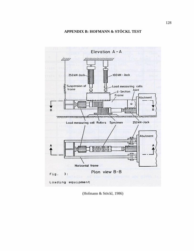
128
APPENDIX B: HOFMANN & STÖCKL TEST
(Hofmann & Stöckl, 1986)