Embed Size (px)
Citation preview

A New Insertion-based Construction Heuristic for Solving the Pickup and Delivery
Problem with Time Windows
Quan Lu
Daniel J. Epstein Department of Industrial and Systems Engineering
University of Southern California
Los Angeles, CA 90089-0193
Maged M. Dessouky**
Daniel J. Epstein Department of Industrial and Systems Engineering
University of Southern California
3715 McClintock Avenue
Los Angeles, CA 90089-0193, USA
Tel. +1 213 740 4891 – Fax +1 213 740 1120
** Corresponding Author

1
A New Insertion-based Construction Heuristic for Solving the Pickup and Delivery
Problem with Time Windows
Abstract
In this paper we present a new insertion-based construction heuristic to solve the multi-
vehicle pickup and delivery problem with time windows. The new heuristic does not
only consider the classical incremental distance measure in the insertion evaluation
criteria but also the cost of reducing the time window slack due to the insertion. We also
present a non-standard measure, Crossing Length Percentage, in the insertion evaluation
criteria to quantify the visual attractiveness of the solution. We compared our heuristic
with a sequential and a parallel insertion heuristic on different benchmarking problems,
and the computational results show that the proposed heuristic performs better with
respect to both the standard and non-standard measures.
Keywords
Construction heuristic; pickup and delivery problem; time windows;

2
1. Introduction
Many core problems arising in logistics and public transit can be modeled as a pickup
and delivery problem with time windows (Savelsbergh and Sol, 1995). In the pickup and
delivery problem with time windows (PDPTW), each transportation request has a pickup
and delivery point and the completion of servicing these points must be performed within
a given time window. Since exact approaches can only solve relatively small sized
problems due to the problem being NP-hard, researchers have resorted to heuristic
algorithms to solve the larger sized problems (Savelsbergh and Sol, 1995; Lu and
Dessouky, 2004).
Insertion heuristics construct feasible schedules by iteratively inserting undetermined
nodes into existing routes. A new route is created if no undetermined node can be
inserted into any existing route. Two decisions need to be made by any insertion
heuristic: the selection of the next insertion node and the selection of the next insertion
spot. Most insertion heuristics use some criteria function, typically based on the
incremental of distance or cost, as a selection rule. By applying different selection rules,
variant insertion heuristics may be generated. Insertion-based procedures are used to
create initial/final solutions in most heuristics for PDPTW because they are fast and still
can produce a quality solution. Hunsaker and Savelsbergh (2002) and Campbell and
Savelsbergh (2004) outline the importance of developing efficient insertion heuristics for
routing and scheduling problems. As stated above, they are the preferred method for
deriving an initial solution in improvement heuristics or meta-heuristics. Furthermore,
because of their computational efficiency and ability to operate in real-time, many of the
commercial routing and scheduling software packages use an insertion-based heuristic for
their solution approach (Palmer et al., 2004).
The focus of this paper is to derive a new insertion-based heuristic for the PDPTW. Our
procedure differs from the classical insertion methods in two aspects. First, the classical
insertion methods typically choose the next insertion by selecting a feasible insertion that
has the minimal increase in travel distance or time, with respect to both the time window
and capacity constraints. They do not directly take into consideration the degree of
3
feasibility when determining which node and location to insert next. This myopic
characteristic prevents the insertion-based heuristic from constructing higher quality
solutions, especially when more restricted feasibility constraints are considered such as
time window constraints. To overcome this myopic characteristic, in this paper, we
propose a new insertion evaluation function, which takes into consideration the increase
of travel time as well as the reduction in the slack in the time window due to the insertion
operation. We refer to the time difference between the time window and the service time
as the slack in the time window. For example, instead of always choosing the node and
location with the lowest cost as the next insertion, it may be better to select an insertion,
which does not use much of the available slack so that more opportunities are left for
future insertions.
Second, in practice, operational planners tend to prefer more visually attractive solutions.
This has been observed and confirmed by researchers who have implemented commercial
routing software for industry. For example, see Poot et al. (2002), Rahimi and Dessouky
(2001), and Sahoo et al. (2005). On the other hand, an investigation of human
performance on the Traveling Salesman Problem (TSP) made by MacGregor and
Ormerod (1996) reports that untrained adults, solving “by eye,” are able to find solutions
that are as good as, or even better than, those produced by a number of well-known
heuristics, not subject to individual differences. Their work reveals that more visually
attractive solutions tend to have less total length of distance. We believe that this may
also be true for more restrictive problems, such as the PDP and PDPTW. To account for
this effect, we develop a non-standard measure to evaluate the visual attractiveness for
the existing routes, called Crossing Length Percentage (CLP), to evaluate the visual
attractiveness. A crossing is defined as a point where two routes intersect each other.
Our proposed insertion heuristic incorporates this non-standard measure to create more
visually acceptable solutions.
The reminder of this paper is organized as follows. The literature on the PDPTW is
reviewed in Section 2. In Section 3, we give the formal definition of the problem studied
in this paper. The whole procedure of the proposed insertion heuristic, including the non-

4
standard quality measure, CLP, is given in Section 4. The computational results are
provided in Section 5. Finally, some concluding comments are made in Section 6.
2. Literature Review
Jaw et al. (1986) adapt the traditional insertion algorithm to the multiple-vehicle dial-a-
ride problem with time windows. The heuristic selects the customers in the order of the
increase of the earliest pickup time, inserts the selected customer into the cheapest
feasible position in the existing routes, or adds an unused vehicle to the problem if no
feasible position is found. Madsen et al. (1996) develop an alternative insertion
algorithm for the dial-a-ride problem.
For the single-vehicle PDPTW, Van der Bruggen et al. (1993) develop a two-phase local
search heuristic algorithm. The construction phase starts with an initial route obtained by
visiting the locations in order of increasing centers of their time window, taking prior and
capacity constraints into account. The initial route may be time infeasible. Then, the
initial route is made feasible by interactively applying an objective function that penalizes
the violation of time windows. The feasible routes obtained in the construction phase are
continually improved in the improvement phase. Both phases use a variable-depth search
built up out of seven basic types of arc-exchange procedures. The method has been
tested on problem instances with up to 50 clients.
Ioachim et al. (1995) propose an approximation algorithm for the multiple-vehicle
PDPTW. The algorithm first creates a set of clusters by solving a reduced multiple-
vehicle PDPTW problem exactly using column generation. Each cluster is a small trip
that visits a set of customers. Finally, a multiple traveling salesman problem is solved to
sequence the clusters into the final routes. The proposed approach is tested on a problem
set with up to 250 customers.
Toth and Vigo (1997) describe a fast and effective parallel insertion heuristic to
determine the schedule of transporting handicapped persons using a fleet of
heterogeneous vehicles. The problem can be considered as a multiple-vehicle PDPTW
with additional real-life operational constraints. They also present a tabu procedure to

5
improve the solution obtained by the insertion algorithm. The proposed approach has
been applied in a DSS (Decision Support System) to plan the vehicle service schedule for
the city of Bologna, Italy.
Savelsbergh and Sol (1998) propose three approximation algorithms derived from their
branch-and-price based optimal algorithm. They use the approximation algorithms to
generate columns for the linear programming relaxation. They observe that creating a
good set of columns in the root is the key issue in finding good solutions. Their
approximation algorithms are tested on problem sets with up to 50 customers.
Nanry and Barnes (2000) present a reactive tabu search approach to solve the multiple-
vehicle PDPTW. The initial routes are created through a greedy insertion method. Then,
a reactive tabu search method with three proposed neighborhoods is used to improve the
initial route. The approach is tested on instances with sizes of 25, 50 and 100 customers,
which were constructed from Solomon’s C1 benchmark problems.
Landrieu et al. (2001) present a probabilistic tabu search to solve the single-vehicle
PDPTW. The algorithm was tested on a class of randomly generated instances.
Li and Lim (2001) propose a metaheuristic for the multiple-vehicle PDPTW. First, a
local optimal is found based on three defined neighborhoods. Then, a simulated
annealing like multiple-restart strategy is applied to escape from the local optimal and a
tabu-list is used to avoid cycling in the search process. The algorithm is tested on the
modifications of each of Solomon’s benchmark problem for VRPTW (56 instances).
Lao and Liang (2002) present a two-phase method for the multiple-vehicle PDPTW. In
the first phase, a new hybrid heuristic that is based on a standard insertion procedure and
sweep procedure is applied to construct the initial solution. In the second phase, a tabu
search method is proposed to improve the solution. The algorithm is also tested on the
instances generated from Solomon’s benchmark problems.
Cordeau and Laporte (2003) describe a tabu search heuristic for the multiple-vehicle dial-
a-ride problem with time windows. They propose a new neighborhood evaluation

6
procedure and give extensive computational results based on randomly generated data
sets.
Dessouky, Rahimi, and Weidner (2003) add an environmental component to the criteria
function of an insertion algorithm for the PDPTW problem in addition to the standard
cost component. Simulation results show that adding the environment component to the
insertion criteria component significantly improves the environmental effect of the
schedule without significantly degrading the cost component.
Diana and Dessouky (2004) present a parallel regret insertion heuristic to solve a large-
scale dial-a-ride problem with time windows. The proposed algorithm is tested on data
sets of 500 and 1000 requests built from data of paratransit service in the Los Angeles
County.
3. Problem Definition
We consider the multiple-vehicle PDPTW as follows. We have n customers that need to
be served, each with a pickup location vi and a delivery location vi+n, i = 1, 2, …, n. The
pickup and delivery requests from a customer must be served by the same vehicle, which
we refer to as the pairing constraint. Each customer’s pickup request must be served
before its delivery request, which we refer to as the prior constraint. There are m
identical vehicles available in the fleet. The capacity of each vehicle is Q, and at any
time the total load in a vehicle cannot exceed Q, which is the capacity constraint.
A time window (Ei, Li) is specified for each location vi, i = 1, 2, …, 2n, where Ei denotes
the earliest time a service can take place and Li denotes the latest time a service can start.
All vehicles must start from a central facility with location v0 and return to location v2n+1
during a common time interval. Location v0 and v2n+1 may be physically the same.
Assume E0 is the common earliest time that all vehicles are ready to depart from depot v0
and L0 is the latest time that a vehicle can leave depot v0. The departure time window for
a vehicle from depot v0 is [E0, L0] and the return time window for a vehicle at depot v2n+1
is [E2n+1, L2n+1], where E2n+1= L2n+1= L0. We assume that waiting at any location vi before

7
Ei is allowed but starting the service after time Li is not allowed. That is, the time window
constraint is violated if the arrival time at any location vi is later than Li.
To summarize, the problem we consider has the above four types of constraints: pairing,
prior, capacity, and time window. The objective is to minimize the total cost, which
includes the fixed vehicle cost and travel cost that is proportional to the travel distance.
In reality, the application of the pickup and delivery problems often involves other
service related constraints, especially when they are applied to transport people. The
common service related constraints include the maximum total duration of the route, the
maximum wait time at a stop, and the maximum ride time that limits the time between
pickup and delivery. Notice that the problem defined above has implicitly taken into
account the maximum total duration of the routes, because by enforcing that a vehicle
cannot leave depot v0 earlier than the time instant E0 and a vehicle has to return to depot
v2n+1 no later than time instant L0, the total duration of any route is no more than L0 - E0.
The maximum ride time constraint is indirectly accounted for by having time windows
for both the pickup and delivery points.
4. Construction Heuristic
Consider the problem defined in Section 3. Assume the travel time between any pair of
locations vi and vj is ti,j, i = 0, 1, 2, …, 2n, 2n+1. We denote by Ai the earliest arrival
time of a vehicle at location vi and Di the earliest departure time of a vehicle at location
vi, where Di = max (Ei, Ai) + di and di is the vehicle’s service time at location vi. Note
that Ai and Di are not constants for customer i, and they are relative to the solution under
construction. The time window constraint is violated if Ai > Li at any location vi. We
maintain two quantities for each assigned location vi: waiting time, Wi, Wi = max (0, Ai–
Ei) and the maximal postponed time interval, Yi, where Wi+Yi indicates the maximal
additional time that can be induced by feasibly inserting other locations before vi in the
current route. Assume all k locations in a route R in sequence are 1r
v , 2r
v , … , kr
v , we

8
compute jrY at each location
jrv , j=1,2,…, k as follows. Figure 1 illustrates different W
and Y values in a route with four locations.
−−=+−
=−=
++1,,...2,1}),,max(min{
),(max
11kkiforWYEAL
kjforEALY
jjjjj
kkk
jrrrrr
rrrr
From the definition of Yi, we know that if vi and vj are two adjacent locations in a route
and location vi precedes location vj, then we have Yi ≤ Yj + Wj.
Next, we give the feasibility checking functions including variables Yi and Wi at each
location vi. Assume that location vi and vj are two adjacent locations in an existing route.
Define 'kA as the earliest arrival time at location vk if inserting it into the current route
between locations vi and vj, 'kA = max (Ai, Ei) +di+ ti,k.
Checking whether it is feasible to insert location vk between location vi and vj amounts to
verifying the following two equations: 'kA ≤ Lk, and max( '
kA , Ek) + dk + tk,j ≤ Aj + Wj +Yj.
4.1. Initial Route Selection
E0 (D0) L0
E1 L1
L2
E3 L3A3
A2
D1 A1
W3=0 and Y3=L3-max(A3, E3) = L3- A3
W2= E2-A2 and Y2=min(L2-E2, Y3)= L2-E2
W1=0 and Y1=min(L1-A1, W2+Y2) = L2-A2
W0=0 and Y0=min(L0-E0, W1+Y1) = L0-E0
Figure 1. An Example of Different Y and W values in a route with four locations
E2 (D2)

9
The m-PDPTW is generally a highly constrained problem, because of the existence of
additional constraints such as pairing constraints, prior constraints, and time window
constraints. In a highly constrained problem, each route can contain only a limited
number of customers. There exist pairs of customers such that the customers in each pair
cannot be in the same route even if the route includes only these two customers.
Some researchers have shown the importance of obtaining the right initial routes (e.g. Liu
and Shen, 1999). A set of “right” initial routes can help to obtain a better assignment for
the remaining customers. When the fleet includes homogeneous vehicles and all the
vehicles are based at a common depot, we create the initial routes by finding a maximal
set of customers, where it is impossible to serve any two customers in this set with a
single vehicle.
To compute the maximal set, we first generate a graph G(GN, GA), where GN is the node
set and GA is the arc set. Each node in GN represents a customer to be served, |GN | = n.
An undirected arc connects the nodes representing customer c1 and c2 in graph G, if and
only if no vehicle can serve customers c1 and c2 in a single route. Then, the problem of
finding a maximal set of exclusive customers equals the problem of finding a maximum
size clique in G, a clique being a subset of the nodes such that each node is connected to
all other nodes of the subset. The Max-Clique problem is a well-known NP-Complete
problem (Brelaz, 1979). We use a simple greedy algorithm to find the largest clique as
follows.
Algorithm 4.1.
Step 1. If all nodes in GN are marked, stop and GN is the largest clique. Otherwise,
arbitrarily select an unmarked node i, i∈GN, which has the highest number of
edges incident with it and set node i as marked.
Step 2. Remove all the nodes from set GN, where there is no edge linking node i and these
nodes directly. Remove all the edges from set GA that are incident with the
removed nodes. Go to step 1.

10
Figure 2 gives an example of finding the maximal clique using Algorithm 4.1. The
original problem is shown in Figure 2(a). First, we select node 1, set it as marked, and
remove node 5 as well as the two arcs incident with node 5. The resulting graph G is
shown in Figure 2(b). Next, we select and mark node 3, remove node 6 as well as the
arc incident with node 6, and the result is shown in Figure 2(c). Finally, we select and
mark nodes 2 and 4 in sequence and get the graph consisting of node 1, node 2, node 3,
and node 4, and they are all marked. Therefore, nodes 1, 2, 3, and 4 are the maximal
clique in the original graph.
The computational complexity of Algorithm 4.1 is O(n2). Since Algorithm 4.1 is fast, we
run Algorithm 4.1 n times with choosing the first marked node as each node belonging to
GN and we select the maximal clique in these n obtained cliques as the final result.
Finally, a set of initial routes is created with each route containing one customer, whose
corresponding node in graph G is in the maximal clique found by Algorithm 4.1.
4.2. Computation of the Insertion Cost
Our objective is to minimize the total travel distance as well as the number of used
vehicles, while obeying the pairing, prior, vehicle capacity and time window constraints.
Hence, we need to take into account both the spatial and temporal aspects of the problem.
The amount of the insertion cost should reflect both the increment of the distance as well
Figure 2. An Example of Using Algorithm 4.1 to Get the Largest Clique
5 3 4
6 2
(a)
1
3*4
2
(c)
1*
3 4
6 2
(b)
1*
3*4*
2*
(d)
1*
11
as the amount of the reduced slack in the time windows. From our knowledge, there has
been no work that considers including in the insertion cost the reduction of the time
window slack due to the insertion. In this section, we propose a new methodology to
compute the insertion cost for the routing problems with hard time window constraints.
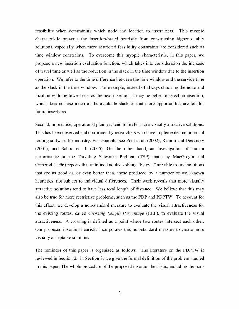
Recall that two quantities, the waiting time (W) and the maximal postponed time (Y), are
associated with each location in a route. Inserting a new location in a route may affect
the W and Y values of the locations before and after the insertion position in the route.
For example, Figure 3(a) gives the W and Y values for each location in a route, which we
refer it as the W-Y graph of the route. Figure 3(b) shows the W-Y graph after inserting a
new location between the third and fourth location in the route. We can conclude the
following three observations from Figure 3.
1. Inserting a new location may decrease the Y value of the locations before the insertion
but not change the W value of the locations before the insertion.
2. The increase of the travel time caused by the insertion is offset by the waiting time at
the locations after the insertion or the maximal postponed time at the last location in
the route.
3. If there is waiting time at the new inserted location, the waiting time can be
considered as being moved from some waiting time after the insertion or the maximal
postponed time from the last location in the route.
New 4
Figure 3. An Example Showing the W-Y Graphs for the Routes before and after the Insertion
3 2 1 6 5
(a) (b)
Waiting Time Maximal Postponed Time
4 3 2 1 6 5

12
Next, we describe how to evaluate the insertion cost. Assume that a route R contains k
locations: 1r
v , 2r
v , …, kr
v . And it is feasible to insert location jrv between location
1−irv
and ir
v in route R. Let 'jrA be the vehicle’s earliest arrival time at location
jrv after
inserting location jrv into route R, ='
jrA ),max(11 −− ii rr EA +di-1+ti-1,j. Let ='
jrW
),0max( 'jj rr AE − and ='
jrY min { −jrL ),max( '
jj rr EA , ∆−+ii rr YW }, where =∆ ti-1,j + tj,i -
ti-1,i + dj + 'jrW . Let the cost of this insertion operation be C. Then, we have C = c1 + c2 +
c3, where c1 represents the decrease of the time window slack of locations 1r
v , 2r
v , …,
1−irv , after inserting location
jrv after location 1−ir
v in route R, c2 represents the decrease of
the time window slack of jrv itself after the insertion, and c3 represents the decrease of
the time window slack of locations ir
v , 1+ir
v , …, kr
v , after inserting location jrv before
location ir
v in route R. To compute c1, we use the following algorithm.
Algorithm 4.2.
Step 0. Let β = 'jrW + '
jrY , c1 = 0, and k = i –1.
Step 1. If β ≥ krY or k = 1, return c1 and stop the algorithm.
Step 2. If k = i –1, let c1 = krY – β and go to step 4. Otherwise, go to step 3.
Step 3. If1+krW > 0, let c1 = c1 + min(
krY – β, 1+krW ).
Step 4. Let β = krW + β and k = k –1. Go to step 1.
We illustrate Algorithm 4.2 with the example shown in Figure 4. Figure 4(a) gives the
W-Y graph of a route with six locations. The W-Y graph after inserting a new location
between locations 5 and 6 is shown in Figure 4(b).
bn
New 4 3 2 1 6 5
(a) (b)
Waiting Time Maximal Postponed Time
4 3 2 1 6 5
b5b4
b3b2 b6

13
Inserting a new location in Figure 4(b) reduces Y5 by b5, Y4 by b4 and Y3 by b3. But we
only count b5 in c1, because reducing Y4 by b4 causes Y5 to decrease by b4 and reducing Y3
by b3 causes both Y4 and Y5 to decrease by b3. Thus, we use b5 to represent the reduction
of the time window slack at locations 3, 4 and 5. Furthermore, the insertion also reduces
Y2 by b2. If Y2 is reduced by b2, this b2 amount of time will be offset by W3 and will not
affect Y3, Y4 and Y5. Therefore, b2 should be considered as an additional lost of slack and
we have c1 = b2 + b5.
Next, we compute the cost of c2 using the following equations. Remember that ='jrW
),0max( 'jj rr AE − and ='
jrY min { −jrL ),max( '
jj rr EA , ∆−+ii rr YW }, where =∆ ti-1,j + tj,i
- ti-1,i + dj + 'jrW and ='
jrA ),max(11 −− ii rr EA +di-1+ ti-1,j. Define c2 = −
jrL −),max( 'jj rr EA
'jrY . The cost of c2 measures the reduction of the time window slack for location vj due to
the small slack in the succeeding locations after the insertion.
Finally, the value of c3 represents the increment of the insertion distance. If the vehicle’s
velocity is constant, the travel distance is proportional to the travel time. Therefore, we
unify the units of all the costs, c1, c2 and c3, to be time here. Formally, we define c3 = ti-1,j
+ tj,i - ti-1,i. In the example in Figure 4, we have c3 = b6.
A large value of c1 implies that from the time windows point of view, it is better to insert
vj at some position before location vi-1, because inserting location vj after location vi-1
makes the arrival time at location vj so close to the time window Lj that the Y values of
some locations before location vi-1 are diminished. On the contrary, a large value of c2
implies that from the time windows point of view, it is better to insert vj at some position
after location vi, because the insertion of vj before vi wastes the significant slack at vj,
−jL ),max( 'jj EA , due to a small slack in the succeeding nodes. Therefore, we have the

14
following property for c1 and c2. If both c1 > 0 and c2 > 0, it implies that the insertion of
vj between vi-1 and vi has significantly increased the travel time that both the Y values at
vi-1 and vi are diminished. We illustrate the above three different cases in Figure 5 (a), (b)
and (c), respectively. Assume that a new location will be inserted between the third and
fourth locations in the route.
4.3. Consideration of the Measure for Visual Attractiveness
In this section, we describe how to embed the non-standard quality criteria, CLP, into our
proposed construction heuristic to improve the quality of the solution.
Figure 5. Three Different Cases for Computing the Insertion Cost
New 4 3 2 1 6 5
(a) c1 = b3 > 0, c2 = 0, and c3 = b4.
5 3 2 1 6 4
b4
b1b2
b5 b6
b3
bn
New 4 3 2 1 6 5
(b) c1 = 0, c2 = bn > 0, and c3 = b4.
5 3 2 1 6 4
b4 b5
b6
New 4 3 2 1 6 5
(a) c1 = b3 > 0, c2 = bn, and c3 = b4.
5 3 2 1 6 4
b4 b1
b2
b5 b6
b3bn

15
Poot et al. (2002), based on their experience on developing the SHORTEREC
Distriplanner® a commercial vehicle routing software for industry, point out that visually
attractive plans seem to be more logical to the operational planners and closer to those
plans created by the human dispatcher. Therefore, producing such plans not only
generates more reasonable solutions for practical routing problems but also helps to
create trust among the planners and drivers in a route planning system, which leads to fast
acceptance of the system.
We can evaluate the visual attractiveness of a solution from two aspects: the visual
attractiveness of each single route and the visual attractiveness of different routes’
geographical relationship. The experiments made by MacGregor and Ormerod (1996)
suggest that visual attractiveness of a single route implicitly reflects the route’s length.
However, no research supports that such a relationship also exists between the
geographical relationship of different routes and the total distance of the solution. For
example, it is visually more attractive to have less requests served by one route contained
in the convex hull of another route, but there is no evidence that indicates that solutions
with less overlap of the convex hulls from different routes are more probable to have less
total distance. An instance of a solution with less overlap from different routes’ convex
hulls having longer total distance can be found in Sahoo et al. (2005). Thus, we only
consider measuring the visual attractiveness of each individual route.
MacGregor and Ormerod (1996) propose the convex-hull hypothesis, which advocates
the use of the convex hull as part of a strategy to create a TSP tour, to explain why a high
quality TSP solution can be found by trying to obtain a visual attractive solution. Rooij
et al. (2003) try to justify the same phenomenon with the hypothesis that people achieve
this by trying to avoid crossings. Namely, the convex-hull hypothesis and the crossings-
avoidance hypothesis are not mutually exclusive. We can always find a more visually
attractive TSP solution by removing the crossings from a non-crossing-free TSP solution.
Comparing two crossing-free solutions for the same TSP, the one closer to the convex
hull is more visually attractive and more probable to have shorter total distance.

16
Next, we propose a measure Crossing Length Percentage (CLP) to evaluate the degree of
crossings with a single trip. Note that the number of crossings alone is not a proper
quantity measure to evaluate the crossing level of a trip, since the crossing level also
depends on how deep the crossings are and whether the multiple crossings entangle each
other. The CLP of a trip is defined as the sum of the crossed length of all the crossings
divided by the total length of the trip. The crossed length of a crossing equals the
minimum total length of the crossing. The CLP value of a trip can be calculated using
the following Algorithm 4.3.
Algorithm 4.3.
Step 1. Assume the total length of a trip is λ. Compute all the n crossing points in the
trip. Let them be cs1, cs2, …, csn.
Step 2. For each crossing point csi, i = 1,2, … n. Calculate the distance βi, where βi
equals the route’s length of the portion within crossing point csi.
Step 3. The CLP value of the trip can be computed as λβλβ /),min(1
i
n
ii∑
=
− .
Next, we illustrate how to apply Algorithm 4.3 to compute the CLP value for the two
trips shown in Figure 6, where we depict each segment’s length next to the segment.
1
Figure 6. Examples of Computing Crossing Length Percentage
(a) (b)
2
4
1
1
4
Depot
DC
E
I
H
F
B
A Length of Segments B-C 0.5 C-D 0.5 D-E 0.5 E-F 0.5 F-B 0.5 B-G 0.5 G-C 0.3 C-E 0.2 E-H 0.5
2
2
3
2
Depot
G

17
The trip in Figure 6(a) contains only one crossing. The CLP value of the trip in Figure
6(a) is min {4+4+2, 1+1+1}/13 = 0.23. The trip in Figure 6(b) contains multiple
crossings. The crossed lengths for the three crossings at points B, C and E in Figure 6(b)
equal BC+CD+DE+EF+FB, CD+DE+EF+FB+BG+GC, and EF+FB+BG+GC+CE,
respectively. And, the sum of the crossed lengths for all these three crossings is
BC+2*CD+2*DE+3*EF+3*FB +2*BG+2*GC+CE = 7.3. Note that the lengths of
segments CD, DE, EF, FB, BG and GC are counted more than once to represent the
entanglement of the crossings. For instance, the length of segments EF and FB are
counted three times because they are contained in all three crossings. The CLP value of
the trip in Figure 6(b) is 7.3/13 = 0.56.
The CLP value measures the visual attractiveness of a single route with crossings.
Maintaining routes with lower CLP at each iteration in an insertion heuristic can avoid
the acceptance of unattractive insertions in the earlier stage of creating interim routes.
Not only does the CLP value indicate whether a trip is visually attractive or not, but it
also indicates the most entangled portion in a visually unattractive trip. A portion in a
trip, which comprises of segments counted the highest number of times in the
computation of the CLP, is more likely to have entanglements. Therefore, to improve a
trip, instead of randomly exchanging the visiting sequence of all the customers in the
entire trip, we need to focus on adjusting the customers’ sequence within the most
entangled portion of the trip. This makes the behavior of each improvement step more
reasonable and closer to what human dispatchers will do.
Next, we discuss in detail how to incorporate the CLP to guide the insertion process. As
pointed out before, crossing avoidance is a common logic behind the human dispatcher
while creating routes. It is easy to find locations to insert without causing any crossings
at the beginning of the insertion because each route contains only a few locations and
many locations are available to be added. As more and more locations are assigned and
the routes become more and more complicated, the dispatching logic changes from
18
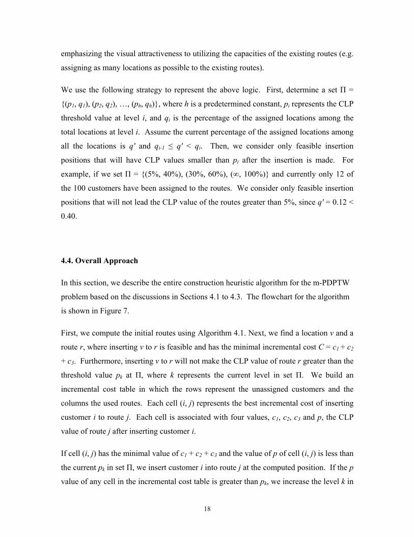
emphasizing the visual attractiveness to utilizing the capacities of the existing routes (e.g.
assigning as many locations as possible to the existing routes).
We use the following strategy to represent the above logic. First, determine a set Π =
{(p1, q1), (p2, q2), …, (ph, qh)}, where h is a predetermined constant, pi represents the CLP
threshold value at level i, and qi is the percentage of the assigned locations among the
total locations at level i. Assume the current percentage of the assigned locations among
all the locations is q' and qi-1 ≤ q' < qi. Then, we consider only feasible insertion
positions that will have CLP values smaller than pi after the insertion is made. For
example, if we set Π = {(5%, 40%), (30%, 60%), (∞, 100%)} and currently only 12 of
the 100 customers have been assigned to the routes. We consider only feasible insertion
positions that will not lead the CLP value of the routes greater than 5%, since q' = 0.12 <
0.40.
4.4. Overall Approach
In this section, we describe the entire construction heuristic algorithm for the m-PDPTW
problem based on the discussions in Sections 4.1 to 4.3. The flowchart for the algorithm
is shown in Figure 7.
First, we compute the initial routes using Algorithm 4.1. Next, we find a location v and a
route r, where inserting v to r is feasible and has the minimal incremental cost C = c1 + c2
+ c3. Furthermore, inserting v to r will not make the CLP value of route r greater than the
threshold value pk at Π, where k represents the current level in set Π. We build an
incremental cost table in which the rows represent the unassigned customers and the
columns the used routes. Each cell (i, j) represents the best incremental cost of inserting
customer i to route j. Each cell is associated with four values, c1, c2, c3 and p, the CLP
value of route j after inserting customer i.
If cell (i, j) has the minimal value of c1 + c2 + c3 and the value of p of cell (i, j) is less than
the current pk in set Π, we insert customer i into route j at the computed position. If the p
value of any cell in the incremental cost table is greater than pk, we increase the level k in

19
set Π by 1 and reselect the cell with the minimal incremental cost. This strategy ensures
that in selecting the next insertion customer and route pair the CLP value criteria does not
dominate the incremental insertion cost. If there exists a customer that cannot be inserted
into any existing route, assign an unused vehicle for this customer. The above steps are
iterated until there are no unassigned customers or there are still some unassigned
customers but all the vehicles in the fleet have been used. In the latter case, the problem
is infeasible.
Assume there are n customers and m vehicles. The construction heuristic requires
checking all the insertion positions for each unassigned customer in each existing route.
The computational complexity of the common insertion heuristic for the pickup and
delivery problem is O(n3) on the condition that the computational complexity to compute
the insertion cost is a constant, O(1). However, in our insertion heuristic the
computational complexity of computing the costs is O(n), where computing the cost
includes computing c1, c2, c3 and p. To compute c1, we use Algorithm 4.2 whose
complexity is O(n). The complexities to compute c2 and c3 both are O(1). The
complexity to compute the new CLP value after inserting two locations is O(n).
Therefore, the complexity of computing the cost for each customer at each location in
each route is O(n) and the total computational complexity for the construction heuristic is
O(n4).

20
Yes
No
Figure 7. Flow Chart of the Overall Construction Heuristic
No Yes
Yes
No
Call Algorithm 4.1 to compute the exclusively served customer set.
Select an unused vehicle and create a new route.
Create new route(s), where each route visits one customer from the exclusively served customer set.
Compute the total cost C for each unassigned customer at each feasible
insertion location in each existing route and the CLP value of the route
after the insertion.
Try to find the customer and route pair that has the minimal C cost and
the CLP value is less than the current qk. Succeed?
Yes
Insert the selected customer into the route
Increase the level k in Π by set k = k +1
k equals h?
Have all the customers been served?
Stop Algorithm
Is there a customer that cannot be inserted in any
existing route?
No
Update the W and Y value at each inserted location.

21
5. Computational Results
Our algorithm was coded in C++ with Standard Template Library and executed on a
personal computer using Pentium III 1.2G processor. We set Π = {(5%, 40%), (15%,
60%), (50%, 80%), (∞, 100%)}. We tested the proposed construction heuristic on the
benchmark problem instances provided by Li and Lim (2001). They generated the data
sets from Solomon’s (1987) vehicle routing benchmark problems consisting of 56
instances by randomly pairing up the customer locations. Li and Lim solved these new
created pickup and delivery instances using a tabu-embedded simulated annealing
algorithm. Since our objective is to develop a new insertion heuristic that can efficiently
construct solutions quickly, we are not trying to beat their results for the following two
reasons. First, their algorithm is much more complex than ours (e.g. their average
computational time is 730 seconds, but ours is 13 seconds). Secondly, their algorithm is
not bounded and sensitive to the data set, but our proposed heuristic is computationally
bounded (their computational time varies from 33 seconds to 4106 seconds, but our
computational time varies from 10 seconds to 23 seconds).
We compared our algorithm with a sequential insertion heuristic algorithm and a parallel
insertion heuristic. The sequential insertion algorithm starts with an initial route, which
consists of only one customer that is closest to the vehicle’s depot. It then searches for
all feasible insertions of the unassigned customers and finds the insertion that results in
the minimum increase of the objective function value. If such an insertion is found, the
customer will be added to the route at the position with the minimal additional cost. If
there exists any customer that is infeasible to insert into any existing routes, create a new
route for this customer. The parallel insertion differs from the sequential insertion
algorithm only at the initial routes generation stage. From our knowledge, there is no
good strategy in the literature on how to choose pivot customers to create the initial
routes for the m-PDPTW. Toth and Vigo (1997) develop a parallel insertion procedure
for the m-PDPTW, in which the number of initial routes is calculated as the minimum
number of vehicles needed to serve 60% of all the requests. However, this strategy is
not suitable for our test data. Therefore, we still use Algorithm 4.1 to select the pivot

22
customers for the initial routes. Notice that for the m-PDPTW, multiple routes are
primarily created because of the time window constraints.
The computational results are shown in Tables 1 and 3. We compared and listed three
measures of the solution quality obtained by the sequential insertion, parallel insertion,
and our proposed construction heuristic: number of used vehicles, total travel time and
average crossing length percentage (CLP) value. We also listed the number of vehicles
and total travel time of the results reported by Li and Lim (2001). We cannot compute
the CLP value from the Li and Lim results since they did not present the complete final
solution (routes) in their paper. Table 1 shows the results on the 19 clustered instances
generated from the C1 and C2 data sets in Solomon’s benchmarking problem. Each
instance in Solomon’s problem has 100 locations, but some instances here have more
than 100 locations because some dummy nodes are added for pairing purposes.
Sequential Insertion Parallel Insertion Proposed Algorithm Li&Lim’s Tabu Search
Prob # of Veh.
Travel Time
Avg. CLP
# of Veh.
Travel Time
Avg. CLP
# of Veh.
Travel Time
Avg. CLP
# of Veh.
Travel Time
LC101 11 867.3 0.00 10 828.9 0.00 10 828.9 0.00 10 828.9 LC102 13 1129.1 0.11 12 1001.9 0.08 11 912.0 0.01 10 828.9 LC103 12 1172.1 0.16 12 1205.5 0.14 11 882.5 0.00 10 827.8 LC104 11 966.1 0.06 11 915.5 0.01 9 861.9 0.01 9 861.9 LC105 12 1037.6 0.07 11 828.9 0.00 10 828.9 0.00 10 828.9 LC106 13 1139.6 0.16 13 1035.6 0.15 10 931.5 0.03 10 828.9 LC107 11 924.8 0.00 11 899.8 0.01 10 828.9 0.00 10 828.9 LC108 12 1247.5 0.33 11 1251.9 0.33 11 1063.5 0.00 10 826.4 LC109 11 1293.8 0.05 11 1273.8 0.05 11 924.5 0.00 10 827.8 LC201 3 591.5 0.03 3 591.5 0.03 3 591.5 0.03 3 591.5 LC202 5 972.3 0.13 4 759.9 0.05 3 663.5 0.02 3 591.5 LC203 4 849.5 0.06 4 822.2 0.06 4 753.5 0.01 3 585.5 LC204 4 954.9 0.02 4 954.9 0.02 3 591.2 0.00 3 591.2 LC205 4 792.0 0.00 4 688.9 0.01 3 592.4 0.00 3 588.9 LC206 4 867.9 0.09 4 841.9 0.07 4 618.3 0.00 3 588.5 LC207 4 709.3 0.00 4 684.5 0.01 3 588.3 0.00 3 588.3 LC208 4 761.5 0.00 4 719.9 0.00 3 629.4 0.00 3 588.3
Table 1. Computational Results of the Four Heuristics on the Clustered
Problems.

23
From Table 1, our proposed heuristic outperforms the sequential heuristic and parallel
heuristic in all the LC100 and LC200 problem instances on each performance measure:
number of used vehicles, total travel time and average CLP values. We summarize the
results in Table 2. The difference of the LC100 and LC200 problems is that the LC100
problems have a shorter scheduling horizon while the LC200 problems have a longer
scheduling horizon (larger time windows). Comparing with the sequential insertion in
the LC100 problems, our proposed heuristic reduced the total travel time by 17%, and the
total CLP value by 94%. Comparing with the parallel insertion in the LC100 problems,
our proposed heuristic reduced the total travel time by 12%, and the total CLP value by
71%. Comparing with the sequential insertion in the L200 problems, our proposed
heuristic reduced the total travel time by 22%, and the total CLP value by 81%.
Comparing with the parallel insertion in the L200 problems, our proposed heuristic
reduced the total travel time by 15%, and the total CLP value by 60%. Therefore, our
heuristic gave a significant improvement for the LC problems regarding the visual
attractiveness measurement, the CLP value. Note that the sequential insertion method
gave better CLP values for the LC200 problems than the LC100 problems because the
sequential insertion heuristic does not take into account the time windows while
performing insertions. Therefore, it performed worse and generated more crossings for
the data sets with tighter time windows (e.g. LC100). Since our insertion procedure
directly accounts for the time windows, the CLP values do not deteriorate with tighter
time windows.
Sequential Insertion Parallel Insertion Proposed Algorithm Li&Lim’s Tabu Search
Prob # of Veh.
Travel Time
Avg. CLP
# of Veh.
Travel Time
Avg. CLP
# of Veh.
Travel Time
Avg. CLP
# of Veh.
Travel Time
LC100 11.8 1086.4 0.11 11.3 1026.9 0.085 10.3 895.8 0.005 9.9 832.0
LC200 4 812.3 0.04 3.88 757.9 0.031 3.3 628.5 0.007 3 589.2
Table 2. Summary of the Computational Results of the Three Heuristics on the Clustered Problems.

24
We also compared our solutions with the solutions reported by Li and Lim (2001). Since
they did not report the CLP value, we only compared the number of used vehicles and the
total travel time. Li and Lim’s heuristic is a tabu-based metaheuristic and their
computational time is sensitive to the data of the problem. For example, their
computational time varies from 33 seconds to 4106 seconds and the average
computational time is about 730 seconds. On the contrary, our proposed heuristic is very
quick and computationally bounded. The longest computational time is only 23 seconds
and the average computational time is around 13 seconds. Furthermore, comparing with
the Li and Lim’s results in the L200 problems, our proposed heuristic’s results are within
8% regarding the total travel time. Comparing the results in the L200 problems, our
proposed heuristic’s results are within 6% regarding the total travel time. Therefore, our
proposed heuristic gave very close results to the Tabu search on the cluster problems with
both loose and tight time window constraints.
In the following Table 3, we provide the computational results of using the three
algorithms in solving the LR100 and LR200 problems. The LR type problems are
randomly distributed problems. Similar as before, the LR100 problems have short
scheduling horizon while the LR200 problems have a longer scheduling horizon.
Sequential Insertion Parallel Insertion Proposed Algorithm Li&Lim’s Tabu Search
Prob # of Veh.
Travel Time
Avg. CLP
# of Veh.
Travel Time
Avg. CLP
# of Veh.
Travel Time
Avg. CLP
# of Veh.
Travel Time
LR101 21 1818.4 0.16 19 1767.4 0.05 19 1749.3 0.05 19 1650.8 LR102 19 1725.9 0.12 19 1602.2 0.03 19 1561.0 0.03 17 1487.6 LR103 16 1683.6 0.36 14 1552.2 0.31 13 1333.2 0.01 13 1292.7 LR104 12 1316.4 0.08 12 1166.8 0.05 11 1109.5 0.02 9 1013.4 LR105 19 1697.0 0.25 16 1449.2 0.04 16 1427.3 0.04 14 1377.1 LR106 17 1619.6 0.39 16 1547.2 0.28 13 1298.1 0.04 12 1252.6 LR107 13 1344.1 0.06 11 1193.6 0.06 10 1111.3 0.00 10 1111.3 LR108 12 1339.5 0.05 12 1306.6 0.05 10 1037.4 0.01 9 968.9 LR109 14 1390.2 0.03 12 1376.6 0.02 12 1263.4 0.00 11 1239.9 LR110 15 1463.9 0.07 12 1227.1 0.07 10 1170.4 0.02 10 1159.3 LR111 13 1306.8 0.09 12 1282.6 0.06 12 1184.7 0.02 10 1108.9 LR112 13 1265.6 0.03 11 1237.4 0.03 10 1058.4 0.01 9 1003.7 LR201 7 1571.5 0.43 6 1492.4 0.28 4 1298.8 0.01 4 1263.8 LR202 7 1611.2 0.58 6 1581.4 0.52 5 1351.4 0.00 3 1197.6 LR203 6 1404.7 0.11 6 1372.5 0.10 4 1067.7 0.00 3 949.4

25
LR204 5 1314.9 0.09 4 1186.8 0.04 2 849.0 0.01 2 849.0 LR205 5 1566.6 0.39 4 1417.7 0.06 4 1210.4 0.02 3 1054.0 LR206 4 1465.0 0.08 4 1524.5 0.07 4 1098.8 0.00 3 931.6 LR207 4 1493.7 0.09 4 1461.7 0.09 4 1135.6 0.03 2 903.0 LR208 4 1437.4 0.00 4 1353.1 0.01 3 908.1 0.01 2 734.8 LR209 4 1378.2 0.31 3 1008.2 0.11 3 937.0 0.00 3 937.0 LR210 5 1532.5 0.44 4 1381.6 0.35 4 1106.4 0.05 3 964.2 LR211 4 1151.4 0.07 4 1162.9 0.07 3 1107.0 0.01 2 907.8
From Table 3, we can conclude that our proposed heuristic outperforms the sequential
heuristic and parallel heuristic in all the LR100 and LR200 problem instances. The
summary of the computational results in Table 3 is shown in Table 4. From Table 4, we
can conclude that comparing with the sequential and parallel insertion algorithm our
proposed heuristic significantly reduces the average CLP values for both the LR100 and
LR200 problem sets. It also reduced the average travel time by 14% and 24% for the
LR100 and LR200 problem sets comparing with the sequential insertion, respectively.
Comparing with the parallel insertion, it reduced the average travel time by 7% and 18%
for the LR100 and LR200 problem, respectively. Comparing with the Li and Lim’s meta-
heuristic, our proposed heuristic’s results are within 4.3% regarding the total travel time
for the LR100 problem sets and are within 12% regarding the total travel time for the
LR200 problem sets.
Sequential Insertion Parallel Insertion Proposed Algorithm Li&Lim’s Tabu Search
Prob # of Veh.
Travel Time
Avg. CLP
# of Veh.
Travel Time
Avg. CLP
# of Veh.
Travel Time
Avg. CLP
# of Veh.
Travel Time
LR100 15.3 1497.6 0.14 13.8 1392.4 0.09 12.9 1275.3 0.02 11.9 1222.1
LR200 5 1447.9 0.23 4.5 1358.4 0.16 3.63 1097.2 0.03 2.72 972.0
Table 3. Computational Results of the Three Heuristics on the Randomly Distributed Problems
Table 4. Summary of the Computational Results of the Three Heuristics on the Randomly Distributed Problems

26
6. Conclusion
We proposed a new insertion-based construction heuristic for solving the m-PDP with
time windows. Our objective was to design a computationally bounded heuristic that
generates high quality solutions in a short time. Furthermore, we investigated how to
quantitatively measure the visual attractiveness of the generated solutions. Visual
attractiveness is a key logic behind the strategy of a dispatcher and a visual attractive
solution can improve the trust between the routing software and planners. A measure,
Crossing Length Percentage, was presented to quantify the visual attractiveness of the
solution. This measure was incorporated in the proposed heuristic to improve the quality
of the solution.
The new heuristic considered the insertion cost that not only includes the classical
incremental distance but also the cost of the reduction of the time window slack due to
the insertions. We compared our heuristic with a insertion heuristic and a parallel
heuristic on different benchmarking problems, and the computational results showed that
the proposed heuristic performed better with respect to both the standard and non-
standard measures. We also compared our heuristic’s results with the results obtained
from a tabu search by Li and Lim (2001). The number of used vehicles and the total
travel time of our heuristic were both close to the best solutions from their tabu search in
both cluster and randomly generated instances.
Acknowledgements
The research reported in this paper was partially supported by the National Science
Foundation under grant DMI-9732878.
27
References
D. Brelaz (1979). New Methods to color the vertices of a graph. Communications of the ACM, 22, 251-256.
A. M. Campbell and M. Savelsbergh (2004). Efficient Insertion Heuristics for Vehicle Routing and Scheduling Problems. Transportation Science, 38(3), 369-378.
J. F. Cordeau and G. Laporte (2003). A Tabu Search Heuristic for the Static Multi-vehicle Dial-a-ride Problem. Transportation Research, 37(B), 579-594. M. M. Dessouky, M. Rahimi, and M. Weidner (2003). Jointly Optimizing Cost, Service, and Environmental Performance in Demand-Responsive Transit Scheduling. Transportation Research Part D: Transport and Environment, 8; 433-465.
M. Diana and M.M. Dessouky (2004). A New Regret Insertion Heuristic for Solving Large-Scale Dial-a-Ride Problems with Time Windows. Transportation Research, 38(B), 539-557.
B. Hunsaker and M. Savelsbergh (2002). Efficient Feasibility Testing for Dial-a-Ride Problems. Operations Research Letters, 30, 169-173.
I. Ioachim, J. Desrosiers, Y. Dumas, M. M. Solomon and D. Villeneuve (1995). A Request Clustering Algorithm for Door-to-door Handicapped ‘Transportation’. Transportation Science, 29(1), 63-78.
J. J. Jaw, A.R. Odoni, H.N. Psaraftis and N.H.M. Wilson (1986). A Heuristic Algorithm for the Multi Vehicle Advance-request Dial-a-ride Problem with time windows. Transportation Research, 20(B), 243-257.
A. Landrieu, Y. Mati and Z. Binder (2001). A Tabu Search Heuristic for the Single Vehicle Pickup and Delivery Problem with Time Windows. Journal of Intelligent Manufacturing, 12, 497-508.
H.C. Lao and Z. Liang (2002). Pickup and Delivery with Time Windows: Algorithms and Test Case Generation. International Journal on Artificial Intelligence Tools (Architectures, Languages, Algorithms), 11(3), 455-472. Q. Lu and M. M. Dessouky (2004). An Exact Algorithm for the Multiple Vehicle Pickup and Delivery Problem. Transportation Science, 38, 503-514.
H. Li and A Lim (2001). A Metaheuristic for the Pickup and Delivery Problem with Time Windows. Proceedings 13th IEEE ICTAI 2001, Los Alamitos, CA, 160-167.
F. H. Liu and S. Y. Shen, S.-Y (1999). A Route-neighborhood-based Metaheuristic for Vehicle Routing Problem with Time Windows. European Journal of Operations Research, 118, 485-504.

28
O.B.G. Madsen, H.F. Ravn and J. M. Rygaard (1996). A Heuristic Algorithm for a Dial-a-ride Problem with Time Windows, Multiple Capacities, and Multiple Objectives. Annals of Operations Research, 60, 193-208. J.N. MacGregor and T. Ormerod (1996). Human Performance on the traveling salesman problem. Perception & Psychophysics, 58(4), 527-539.
D. Marco and M. Dessouky (2002). A New Regret Insertion Heuristic for Solving Large-scale Dial-a-ride problems with Time Windows. Working Paper, University of Southern California.
W. P. Nanry and J. W. Barnes (2000). Solving the Pickup and Delivery Problem with Time Windows Using Reactive Tabu Search. Transportation Research, 34B(2), 107-121.
M. Rahimi and M. Dessouky (2001). A Hierarchical Task Model for Dispatching in Computer-Assisted Demand-Responsive Paratransit Operation. ITS Journal, 6, 199-223.
K. Palmer, M. M. Dessouky, T. Abdelmaguid (2004). Impacts of Management Practices and Advanced Technologies on Demand Responsive Transit Systems. Transportation Research, Part A; Policy and Practice, 38, 495-509.
A. Poot, G. Kant, and A.P.M. Wagelmans (2002) A Savings Based Method for Real-life Vehicle Routing Problems, Journal of the Operational Research Society, 53, 57-68.
I. Rooij, U. Stege, and A. Schactman (2003) Convex Hall and Tour Crossings in the Euclidean Traveling Salesperson Problem: Implications for Human Performance Studies. Memory & Cognition, 31(2), 215-220.
M. W. P. Savelsbergh and M. Sol (1995) The General Pickup and Delivery Problem. Transportation Science, 29(1), 17-29.
M. W. P. Savelsbergh and M. Sol (1998). Drive: Dynamic Routing of Independent Vehicles. Operations Research, 46 (4), 474-490.
M. M. Solomon, (1986). On the Worst-case Performance of some Heuristics for the Vehicle Routing and Scheduling Problem with Time Window Constraints. Networks, 16(2), 161-174.
M. M. Solomon (1987). Algorithms for the Vehicle Routing and Scheduling Problems with Time Window Constraints. Operations Research, 35(2), 254-265.
S. Sahoo, S. Kim, and B. Kim (2005). Routing Optimization for Waste Management, Interfaces, to appear in the Special issue for 2004 Franz Edelman Award for Management Science Achievement Competition.
P. Toth and D. Vigo, (1997). Heuristic Algorithm for the Handicapped Persons Transportation Problem. Transportation Science, 31(1), 60-71.
29
L.J.J. Van der Bruggen, J.K. Lenstra and P.C. Schuur (1993). Variable-depth Search for the Single Vehicle Pickup and Delivery Problem with Time Windows. Transportation Science, 27, 298-311.