* Corresponding author. Tel: +39 02.23995906. E-mail address: maurizio.bruglieri@polimi.it

Heuristic algorithms for the operator-based relocation

problem in one-way electric carsharing systems

Maurizio Bruglieria,*

, Ferdinando Pezzellab, Ornella Pisacane

c

a Dipartimento di Design, Politecnico di Milano, Milano, Italy bDipartimento di Ingegneria dell'Informazione,Università Politecnica delle Marche, Ancona,

Italy cFacoltà di Ingegneria, Università degli Studi e-Campus, Novedrate (Como), Italy

Abstract

This paper addresses an Electric Vehicle Relocation Problem (E-VReP), in one-

way carsharing systems, based on operators who move through folding bicycles be-

tween a delivery request and one of pickup. In order to deal with its economical sus-

tainability, a revenue associated with each relocation request satisfied and a cost due

to each operator used are introduced. The new optimization objective maximizes the

total profit. To overcome the drawback due to the high CPU time required by the

Mixed Integer Linear Programming formulation of the E-VReP, four heuristics, also

based on general properties of the feasible solutions, are designed. Their effectiveness

is tested on two sets of realistic instances. In the first one, all the requests have the

same revenue. In the second one, the revenue of each request has a variable compo-

nent related to the user’s rent-time and a fixed one related to the customer satisfaction.

Finally, a sensitivity analysis is carried out on both the number of requests and the

fixed revenue component.

Keywords: carsharing, operator based relocation, economical sustaina-

bility, pickup and delivery problem with time windows, heuristics,

mixed integer linear programming

1 Introduction and literature review

Carsharing consists in the shared use of cars made available under the payment of a

fare according to the time of use. It differs from car rental service since it provides for

the use of the car only for a short time (usually for a fraction of an hour) in order to

favor the sharing of each car among different people during the same day. Due to

environmental sustainability issue, nowadays, several carsharing companies are

providing the customers with the use of Electric Vehicles (EVs) rather than of tradi-

tional internal combustion engine cars. Real-life cases of electric carsharing systems

are given by: Car2Go (http://www.car2go.com/) in Amsterdam and Vienna, for ex-

ample; Autolib (www.autolib.eu) in Paris; Autobleue (http://www.auto-bleue.org) in

Nice-Côte d’Azur (France).

The planning and the management of a carsharing service poses some important

decision problems. About the planning, two significant issues concern the sizing of

the fleet and the location of the parking stations (Cucu et al., 2009; Correia and An-

tunes, 2012; Jorge and Correia, 2013). About the management, some carsharing ser-

vices permit one-way trips, which allow the user to pick up the vehicle in one station,

and return it in another one. The flexibility offered by a one-way system makes it

more attractive to users. But, on the contrary, it is harder to be managed since it in-

volves a possible unbalancing between the demand and the availability of vehicles or

vice versa between the request for returning the vehicles and the availability of vacant

parking lots, making necessary a vehicle relocation. In such cases, the service provid-

er has to develop strategies to relocate the vehicles and restore an optimal distribution

of the carsharing fleet. Such strategies depend also on the available data and the main

objective of the relocation. Barth and Todd (1999) propose the classification in: static

relocation, based on the immediate needs of a particular parking lot; historical predic-

tive relocation, based on an estimation of the requests made using historical data of

the service or techniques of travel demand estimation; exact predictive relocation,

based on the perfect knowledge of the request (like in the case of a carsharing service

on reservation).

The vehicle relocation can be carried out by the user herself or by the service pro-

vider (Barth et al., 2004). In the first case, the user is motivated to car pool or to

choose another parking station or reservation time (generally through the pricing lev-

er); in the second case, the vehicles are moved by personnel either by trucks or direct-

ly driving each of them.

However, in general, operating with EVs rather than the traditional internal com-

bustion engine ones complicates a lot the management of such systems as shown in

Touati-Moungla and Jost (2012). In particular, the authors revise several problems

related to the EV management (e.g., the poor battery range) from an optimization

point of view. The carsharing service offered in the same location is studied also by

Hafez et al. (2011), which, among the other things, minimize, the total travel time of

relocation, through three different heuristics. Jung et al. (2014) address the problem of

locating infrastructure for EVs (i.e., electric taxis in their case) by proposing a new

model where the passenger demand is not known a-priori leading to a stochastic dy-

namic itinerary for each EV.

Kek et al. (2009) design a system based on a three-step optimization-trend-

simulation for supporting carsharing operators in relocating the vehicles. Such a sys-

tem is tested considering a realistic scenario of a carsharing company in Singapore.

Di Febbraro et al. (2012) model the complex dynamics of the carsharing system,

using a discrete event system simulation. The paper considers the relocation made by

both users and staff, and has a twofold objective: reducing the number of required

staff and minimizing the number of carsharing vehicles to satisfy the system demand.

Correia et al. (2014) study the flexibility of the one-way carsharing systems and

they propose a new mathematical formulation including the possibility that a user

selects the station according to its vehicle availability and not only to the distance

from her origin/destination. A real life case study, in Lisbon, is taken into account

during the experimental campaign.

3

Very recent studies have been carried out in the work of Nourinejad and Roorda

(2014) where the authors propose both a-priori benchmark model and a dynamic ve-

hicle relocation optimization model. The latter is solved via a discrete-event simulator

where the arrival of a user request constitutes an event. The numerical results dis-

cussed have shown that the optimization-simulation based model is suitable to deter-

mine a trade-off between the vehicle relocation time and the fleet size.

For the EV relocation problem, Bruglieri et al. 2014(a), propose therefore the use

of a staff of workers that move easily and in eco-sustainable way from a delivery

point to a pickup point by means of a folding bicycle that can be loaded in the trunk

of the EV which needs to be moved. Such a new relocation approach generates a chal-

lenging pickup and delivery problem with features that have been never considered in

the literature. We refer to such a problem as the Electric Vehicle Relocation Problem

(E-VReP )1. E-VReP shares some features with the 1-skip vehicle routing problem

(Archetti and Speranza, 2004) and with the rollon-rolloff problem (Aringhieri et al.,

2004). In particular, in all the three problems, only one item at time is assumed to be

picked up and delivered. Moreover, the routes have to start from and end in a single

depot without exceeding a given maximum time duration.

However, E-VReP is more challenging than the above mentioned problems since

the distance covered by a vehicle depends also on the item picked up, i.e., the residual

electrical charge of the EV picked up. In Bruglieri et al. (2014a), a Mixed Integer

Linear Programming (MILP) formulation of the E-VReP is provided together with

some techniques to speed up its solution.

We remark that in the E-VReP the set of delivery requests and of pickup requests

are supposed to be known in advance and therefore, they are considered as input of

the problem. This assumption is realistic because in the case of a carsharing system on

reservation, it is possible to know a priori the real needs of EV relocation according

to the fleet size, the parking size and the reserved carsharing demand. On the contrary

(i.e. without reservations), the demand can be forecasted through different models and

techniques proposed in the literature and mainly derived from studies in Logistics. For

instance, Cucu et al. (2010) study a forecasting model to exploit customers’ prefer-

ences so as to anticipate their needs and relocate the vehicles accordingly. Wang et al.

(2010) propose an aggregated model at the station level for forecasting the total num-

ber of vehicles rented out and returned over time at each station.

In Bruglieri et al. 2014(b) real world alike instances of the E-VReP are created

through a simulator applied to some data yielded by the Milano transport agency

AMAT and by the main energy supplier company in Milano, A2A (www.a2a.eu ).

The aim of our paper is completely different from Bruglieri et al. 2014(a) since we

want to investigate the economical sustainability of the EV relocation approach intro-

duced in the latter where this aspect was neglected. This is important in order to un-

derstand the practicability of the E-VReP especially from the carsharing managers’

point of view. To deal with the economical sustainability, we introduce the costs re-

lated to the use of the operators and a revenue associated with each relocation request

1 We have changed the acronym of the problem from E-VRP (given in the previous works) to

E-VReP to avoid ambiguity with the Electric Vehicle Routing Problem.

satisfied. While, the original problem aims to handle as many requests as possible

(neglecting the worker costs), the new problem, defined in Section 2 of this paper,

wants to maximize the total profit.

However, this new problem reveals to be more challenging than the original E-

VReP, and therefore, we design four heuristic approaches. Heuristic approaches were

not in depth investigated in the previous works related to the E-VReP and then, they

constitute an innovative contribution of this paper. The first two heuristics are greedy

algorithms that consider the next request to be served according to the criterion of the

nearest neighborhood and of the highest urgency, respectively (Section 3). The third

algorithm is a more structured heuristic that iteratively builds the solution inserting a

pair of compatible (pickup and delivery) requests at the time (Section 4). The policy

followed to couple a pickup request with a delivery one consists in the minimum dis-

tance, while the priority order used to insert the next pair of requests in the route is

guided by the so-called Critical Factor which is an indicator of the difficulty to serve

a request if further delayed. At last the position where the pair of requests is inserted

in the current route, is determined exploiting a proposition that guarantees when an

insertion is feasible and another one that allows a-priori to compute the time extension

due to such an insertion. The proofs of such propositions represent also original con-

tributions of this paper. The forth heuristic is a randomized version of the third one.

We test the effectiveness of the four heuristics on a set of benchmark instances, al-

ready proposed in literature, inspired to a real word context (in the city of Milano).

These results are compared to those provided by two MILP formulations (Section 5).

Moreover, to test the economical sustainability issue, we build a new set of instances

where the revenue associated with each relocation request depends on two compo-

nents: a variable one, proportional to the rent-time of the request (i.e., the time in

which the customer associated with the request uses the carsharing service) and a

fixed one. The latter allows modeling a “future revenue” related to the customer satis-

faction since a satisfied customer will (likely) ask for the service also in the future.

To experiment with the economical sustainability, we also perform a sensitivity

analysis varying the two main input parameters of the E-VReP, i.e., the number of

requests (instance size) and the fixed revenue component associated with each reloca-

tion request (Section 6). Finally, we draw some conclusions and future works (Section

7).

2 E-VReP definition and extension

We recall the description and the notation already used in literature for the E-

VReP. A one-way carsharing service with a homogeneous fleet of EVs is given. Let L

be the maximum distance that an EV can cover when its battery is fully charged. Such

a distance depends on the kind of EV considered (in the experimental campaign we

assume that L =150 km). When the battery of an EV is not fully charged, the maxi-

mum distance that can be covered is assumed to be linearly proportional to the residu-

al charge of the battery (i.e. an EV with residual charge at 50% can cover L/2 km).

Concerning the battery recharging at a station, we can assume that the battery charge

level increases linearly with the time. Let Г indicate the time to fully recharge a com-

5

pletely exhausted battery. We suppose that every EV is always picked up and re-

turned to a parking station lot equipped with a recharge dock so as it is recharged

when it is not used. Since in a one-way carsharing service the cars can be returned to

parking stations different from those where they are picked up, some of them need to

be moved in order to prevent that a station runs out of either EVs or parking lots.

Let D be the set of delivery requests (i.e., the requests of EVs to deliver in order to

prevent that a station runs out of EVs) and let P be the set of pickup requests (i.e.

requests of EVs that need to be moved to vacant parking lots). Each relocation request

𝑟 ∈ 𝑃𝑈𝐷 is characterized by a parking location 𝜈𝑟, i.e., a node of the road network,

by the residual charge of the battery 𝜌𝑟 and by a time window [𝜏𝑟𝑚𝑖𝑛 , 𝜏𝑟

𝑚𝑎𝑥] where

𝜏𝑟𝑚𝑖𝑛 and 𝜏𝑟

𝑚𝑎𝑥 represent respectively the earliest time and the latest time when is

allowed to carry out the request 𝑟. For instance if 𝑟 is a pickup request then 𝜏𝑟𝑚𝑖𝑛 is

the time before which the EV is not available while 𝜏𝑟𝑚𝑎𝑥 is the time after which pick-

ing up the EV is not convenient (since from 𝜏𝑟𝑚𝑎𝑥 it may be used by some other cus-

tomer). For a delivery request 𝑟, 𝜌𝑟 indicates the minimum charge level that the EV

battery must have at time 𝜏𝑟𝑚𝑎𝑥. Therefore, if an EV is delivered before 𝜏𝑟

𝑚𝑎𝑥, the

charge level of its battery may be less than 𝜌𝑟. This is allowed on condition that at

least 𝜌𝑟 is achieved at 𝜏𝑟𝑚𝑎𝑥 , considering that its battery is recharged after the deliv-

ery. Whereas for a pickup request 𝑟, 𝜌𝑟 indicates the battery charge level at 𝜏𝑟𝑚𝑖𝑛 .

Since the fleet of EV is homogeneous each delivery request can be satisfied picking

up every EV of a pickup request on condition that it is compatible for time windows

and battery charge level. Given a team of K workers which leave a single depot, even

at different times, using folding bicycles, we want to determine their routes and

schedules in such a way that the objective to maximize is the number of satisfied re-

quests. Each route consists of an alternating sequence of pickup requests and delivery

requests, such that its duration does not exceed a given threshold T (i.e., the duty time

of the workers), it ends at the depot and both the time windows and battery charge

level constraints are respected. This is the original statement of the E-VReP.

To deal with the economical sustainability of the E-VReP, we change its objective

assuming that a revenue revi is associated with each relocation request i satisfied and

a cost C is associated with each worker used. Thus, the E-VReP objective is modified

into the maximization of the total profit given by the difference between the total

revenue, represented by the sum of the revenues of all the relocation requests satis-

fied, and the total cost, obtained multiplying by C the number of the workers used in

the fixed time horizon. The recharging cost is not directly considered because it can

be assumed fixed. In fact, the carsharing companies usually pay a fixed monthly fee

to the electric energy providers that is proportional to their fleet size (being this a

measure of the electricity consumption). Moreover, through the new objective, we

obtain an extension of the original E-VReP since the previous objective can be ob-

tained again setting C = 0 and revi =1 for every relocation request 𝑖 ∈ 𝑃𝑈𝐷. All the

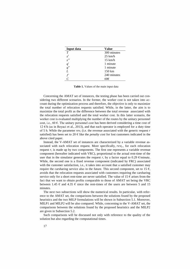
input parameters used by the E-VReP are summarized in Table 1.

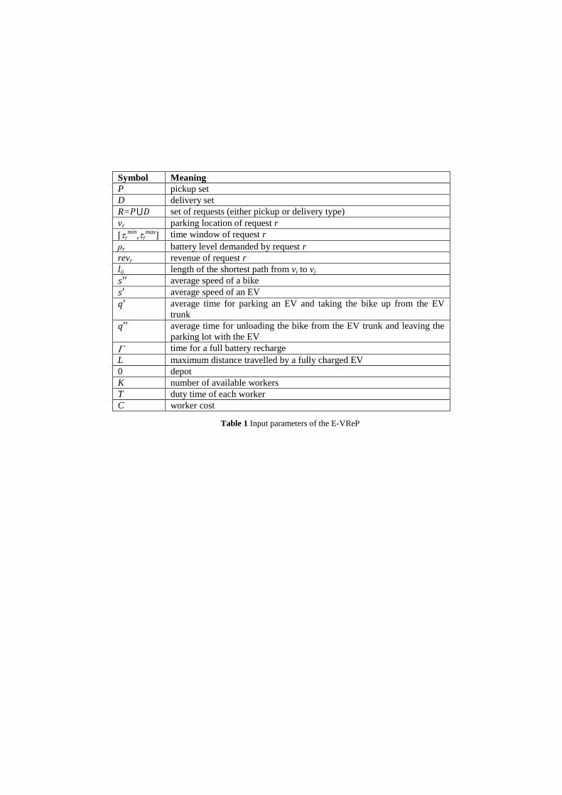
Symbol Meaning

P pickup set

D delivery set

R=𝑃⋃𝐷 set of requests (either pickup or delivery type)

vr parking location of request r

[rmin

,rmax

] time window of request r

ρr battery level demanded by request r

revr revenue of request r

lij length of the shortest path from vi to vj

𝑠′′ average speed of a bike

𝑠′ average speed of an EV

𝑞′ average time for parking an EV and taking the bike up from the EV

trunk

𝑞′′ average time for unloading the bike from the EV trunk and leaving the

parking lot with the EV

time for a full battery recharge

L maximum distance travelled by a fully charged EV

0 depot

K number of available workers

T duty time of each worker

C worker cost

Table 1 Input parameters of the E-VReP

7

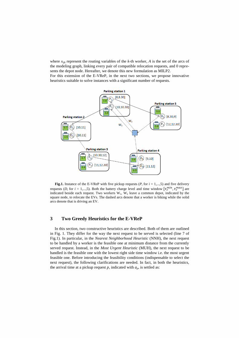
An instance of the problem with five delivery requests and five of pickup is

depicted in Fig. 1. In this example, it is assumed C = 30 €, a duty time equal to 4

hours for each worker, a revenue of 10 € for each request satisfied, a travel time (by

EV) between each pair pickup-delivery of 20 minutes and a travel time (by bike) be-

tween each pair delivery-pickup of 30 minutes. Fig. 1 shows the optimal solution of

the original E-VReP where the number of workers used is 2 and therefore, the total

cost is equal to 60 €. Since six requests are satisfied, the total profit is zero. This be-

havior is due to the fact that the original E-VReP aims to maximize the number of

requests served. While, the optimal solution of the new problem introduced in this

paper consists of only the route performed by the operator W1. Although fewer re-

quests are satisfied, the total profit is not zero but equal to 10 €.

Hereafter the MILP formulation of the E-VReP proposed by Bruglieri et al.

2014(a) is denoted as MILP1. To model the economical sustainability issue, we

change the objective function of MILP1 in the following way:

K

k Aj

ojk

K

k iAji

ijki xCxrev1 ),0(1 0:),(

max (1)

where xijk represent the routing variables of the k-th worker, A is the set of the arcs of

the modeling graph, linking every pair of compatible relocation requests, and 0 repre-

sents the depot node. Hereafter, we denote this new formulation as MILP2.

For this extension of the E-VReP, in the next two sections, we propose innovative

heuristics suitable to solve instances with a significant number of requests.

Fig.1. Instance of the E-VReP with five pickup requests (Pi for i = 1,...,5) and five delivery

requests (Di for i = 1,...,5). Both the battery charge level and time window [𝜏𝑟𝑚𝑖𝑛 , 𝜏𝑟

𝑚𝑎𝑥] are

indicated beside each request. Two workers W1, W2 leave a common depot, indicated by the

square node, to relocate the EVs. The dashed arcs denote that a worker is biking while the solid

arcs denote that is driving an EV.

3 Two Greedy Heuristics for the E-VReP

In this section, two constructive heuristics are described. Both of them are outlined

in Fig. 1. They differ for the way the next request to be served is selected (line 7 of

Fig.1). In particular, in the Nearest Neighborhood Heuristic (NNH), the next request

to be handled by a worker is the feasible one at minimum distance from the currently

served request. Instead, in the Most Urgent Heuristic (MUH), the next request to be

handled is the feasible one with the lowest right side time window i.e. the most urgent

feasible one. Before introducing the feasibility conditions (indispensable to select the

next request), the following clarifications are needed. In fact, in both the heuristics,

the arrival time at a pickup request p, indicated with ap, is settled as:

9

𝑎𝑝 = 𝑎𝑑−1 + 𝑤𝑑−1 + 𝑞′ +𝑙𝑑−1𝑝

𝑠′′ (2)

where d-1 denotes the request of delivery previously served (for the remaining nota-

tion refer to Table 1). While, the arrival time at a delivery request d is fixed as

𝑎𝑑 = 𝑎𝑝 + 𝑤𝑝 + 𝑞′′ +𝑙𝑝𝑑

𝑠′ (3)

where p is the request of pickup previously served.

When the request p is the first inserted, d represents the depot and a0 is set as

𝑎0 = 𝜏𝑝𝑚𝑖𝑛 −

𝑙0𝑝

𝑠′′ (4)

The waiting time wd to satisfy a delivery request d is given by:

𝑤𝑑 = max {0, 𝜏𝑑𝑚𝑖𝑛 − 𝑎𝑑 − 𝑞′} (5)

while the waiting time wp to satisfy a pickup request p, is given by:

𝑤𝑝 = max{0, 𝜏𝑝𝑚𝑖𝑛 − 𝑎𝑝} (6)

The slight asymmetry in the two kinds of waiting times is due to the fact that the de-

livery can start at 𝜏𝑑𝑚𝑖𝑛 − 𝑞′ to deliver the EV exactly at 𝜏𝑑

𝑚𝑖𝑛, while the EV cannot be

picked up at 𝜏𝑝𝑚𝑖𝑛 − 𝑞′′ since it is not available yet.

In both NNH and MUH, the generic request r to handle is selected among the ones

that satisfy the following necessary and sufficient feasibility conditions.

Case 1- The request previously handled by the worker is of delivery, then 𝑟 = 𝑝 ∈𝑃. The following two conditions have to hold:

𝑎𝑝 ≤ 𝜏𝑝𝑚𝑎𝑥 (7)

max{𝑎𝑝, 𝜏𝑝𝑚𝑖𝑛} + 𝑞′′ + min𝑑∈�̃� {

𝑙𝑝𝑑

𝑠′′ +𝑙𝑑0

𝑠′′ } + 𝑞′ − 𝑠𝑡𝑎𝑟𝑡𝜔 ≤ 𝑇 (8)

where �̃� denotes the set of delivery requests compatible with p not yet served. The

condition (7) ensures that the request p is satisfied within the latest allowed time and

condition (8) guarantees that the duration of the route does not exceed the threshold T.

Case 2-The request previously handled by the worker is of pickup (let us indicate it

by p), then 𝑟 = 𝑑 ∈ 𝐷. The following four conditions have to hold:

𝑎𝑑 ≤ 𝜏𝑑𝑚𝑎𝑥 (9)

max{𝑎𝑑 , 𝜏𝑑𝑚𝑖𝑛} + 𝑞′ +

𝑙𝑑0

𝑠′′ − 𝑠𝑡𝑎𝑟𝑡𝜔 ≤ 𝑇 (10)

min {𝜌𝑝 +𝑎𝑝+𝑤𝑝−𝜏𝑝

𝑚𝑖𝑛

Γ, 1} −

𝑙𝑝𝑑

𝐿≥ 0 (11)

min {𝜌𝑝 +𝑎𝑝+𝑤𝑝−𝜏𝑝

𝑚𝑖𝑛

Γ, 1} −

𝑙𝑝𝑑

𝐿+

𝜏𝑑𝑚𝑎𝑥−𝑎𝑑

Γ≥ 𝜌𝑑 (12)

The conditions (9) and (10) work like conditions (7) and (8), respectively. Condition

(11) ensures that the current battery level is sufficient to go from 𝑣𝑝to 𝑣𝑑 along the

minimum path. Condition (12) guarantees that an EV is delivered with a battery level

such that at the time 𝜏𝑑𝑚𝑎𝑥 a charge level not lower than 𝜌𝑑 is reached. If the size of

the pickup set P is not equal to the size of the delivery set D, then both the greedy

heuristics end as soon as no further element in the smallest of these two sets, can be

inserted into a route. Thus, some requests belonging to the biggest of the two sets are

sacrificed in greedy way.

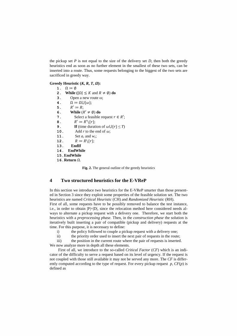
Greedy Heuristic (K, R, T, Ω):

1. Ω ≔ ∅

2. While (|Ω| ≤ 𝐾 and 𝑅 ≠ ∅) do

3. Open a new route ;

4. Ω ≔ Ω⋃{𝜔};

5. 𝑅′ ≔ 𝑅;

6. While (𝑅′ ≠ ∅) do

7. Select a feasible request 𝑟 ∈ 𝑅′; 8. 𝑅′ ≔ 𝑅′\{𝑟}; 9. If (time duration of 𝜔⋃{𝑟} ≤ T)

10. Add r to the end of 𝜔;

11. Set ar and wr;

12. 𝑅 ≔ 𝑅\{𝑟}; 13. EndIf

14. EndWhile

15.EndWhile

16.Return Ω.

Fig. 2. The general outline of the greedy heuristics

4 Two structured heuristics for the E-VReP

In this section we introduce two heuristics for the E-VReP smarter than those present-

ed in Section 3 since they exploit some properties of the feasible solution set. The two

heuristics are named Critical Heuristic (CH) and Randomized Heuristic (RH).

First of all, some requests have to be possibly removed to balance the test instance,

i.e., in order to obtain |P|=|D|, since the relocation method here considered needs al-

ways to alternate a pickup request with a delivery one. Therefore, we start both the

heuristics with a preprocessing phase. Then, in the construction phase the solution is

iteratively built inserting a pair of compatible (pickup and delivery) requests at the

time. For this purpose, it is necessary to define:

i) the policy followed to couple a pickup request with a delivery one;

ii) the priority order used to insert the next pair of requests in the route;

iii) the position in the current route where the pair of requests is inserted.

We now analyze more in depth all these elements.

First of all, we introduce to the so-called Critical Factor (CF) which is an indi-

cator of the difficulty to serve a request based on its level of urgency. If the request is

not coupled with those still available it may not be served any more. The CF is differ-

ently computed according to the type of request. For every pickup request p, CF(p) is

defined as

11

𝐶𝐹(𝑝) = max𝑑∈�̃�

{𝜏𝑑𝑚𝑎𝑥 − 𝑡𝑝𝑑} − 𝜏𝑝

𝑚𝑖𝑛 (13)

where �̃� indicates the set of delivery requests compatible with p not yet served and

𝑡𝑝𝑑 , the time necessary to go from 𝑣𝑝 to 𝑣𝑑 . Since max𝑑∈�̃�{𝜏𝑑𝑚𝑎𝑥 − 𝑡𝑝𝑑} represents

the latest departure time from the location of request p in order to serve a feasible

(unserved) delivery request, the smaller the gap with 𝜏𝑝𝑚𝑖𝑛 is, the more urgently the

request needs to be served. In fact, if the delivery request which the maximum is

achieved with, is no longer available then the request may remain without the possi-

bility to be coupled with a delivery one (since it becomes more unlikely to satisfy the

time window constraint). Similarly, for a delivery request d, CF(d) is defined as

𝐶𝐹(𝑑) = 𝜏𝑑𝑚𝑎𝑥 − min

𝑝∈�̃�{𝜏𝑝

𝑚𝑖𝑛 + 𝑡𝑝𝑑} (14)

where �̃� indicates the set of pickup requests compatible with d not yet served.

The feasibility of requests p and d is checked through the following three neces-

sary conditions:

𝜏𝑝𝑚𝑖𝑛 + 𝑡𝑝𝑑 + 𝑞′′ + 𝑞′ ≤ 𝜏𝑑

𝑚𝑎𝑥 (15)

𝜌𝑝 −𝑙𝑝𝑑

𝐿+

𝜏𝑑𝑚𝑎𝑥−𝜏𝑑

𝑚𝑖𝑛

𝛤≥ 𝜌𝑑 (16)

𝑡0𝑝 + 𝑡𝑑0 + 𝑚𝑎𝑥{𝑡𝑝𝑑 + 𝑞′′, 𝜏𝑑𝑚𝑖𝑛 − 𝜏𝑝

𝑚𝑎𝑥} + 𝑞′ ≤ 𝑇 (17)

The condition (15) is necessary to the respect of the time window of d considering the

departure from vp at τpmin

. Condition (16) is necessary to the battery level feasibility.

In fact, if it is violated, then the battery level ρd cannot be achieved at τpmax

since the

maximum time that can elapse between the pickup request and the delivery one is

equal to τpmax

- τpmin

. Condition (17) is necessary in order to guarantee that the duty

time T of the operators is never exceeded. In this phase of the algorithm, we cannot

guarantee that the pair of requests p and d is feasible because the arrival time and the

waiting time at vp and vd have not been fixed yet. For this reason, we cannot check if

they also satisfy the sufficient feasibility conditions (9)-(12).

The requests with a negative CF have to be removed since infeasible with regard to

their time windows.

The preprocessing phase consists in the following steps for both the two heuristics:

1. the requests are sorted by increasing values of CF;

2. if |P|>|D| then the first |P|-|D| pickup requests are removed;

3. otherwise, if |D|>|P|, the first |D|-|P| delivery requests are removed.

The removed requests will be not handled since they are considered rejected.

Concerning items i) and ii) of the construction phase, at each iteration, the CH

heuristic selects the most critical request (p or d), i.e. the one with minimum value of

CF, and couples it with the request (d or p) satisfying the necessary feasible condi-

tions (15)-(17), whose parking is at minimum distance. If any request cannot be cou-

pled with the currently critical one, the latter will be removed.

Once the first pair (p1, d1) to be inserted has been detected, the route is initialized

with ={0, p1, d1, 0}. Besides, the arrival and the waiting times of the requests p1 and

d1 are initialized in the following way:

𝑎𝑝1 = 𝑚𝑖𝑛 {𝜏𝑝1𝑚𝑎𝑥 , 𝜇 − 𝑡𝑝1𝑑1 − 𝑞′ − 𝑞′′} (18)

where

𝜇 = max {𝜏𝑑1𝑚𝑖𝑛 , 𝜏𝑝1

𝑚𝑖𝑛 + 𝑡𝑝1𝑑1 + 𝑞′ + 𝑞′′} (19)

and

𝑤𝑝1 = 0 (20)

𝑎𝑑1 = 𝑎𝑝1 + 𝑡𝑝1𝑑1 + 𝑞′ + 𝑞′′ (21)

𝑤𝑑1 = 𝜇 − 𝑎𝑑1 (22)

This particular setting guarantees time window feasibility and null waiting time at vd1

if 𝜏𝑝1𝑚𝑎𝑥 is large enough i.e. if 𝜏𝑑1

𝑚𝑖𝑛 − 𝑡𝑝1𝑑1 − 𝑞′− 𝑞′′ ≤ 𝜏𝑝1𝑚𝑎𝑥. More in general, given

a feasible route ={0, p1, d1, p2, d2,…, pn, dn, 0} and a pair (p,d) that has to be insert-

ed between di-1 and pi, the arrival time and the waiting time of p and d are set by the

CH heuristic as in (2), (3), (5), (6).

The main idea beside these equations is to fix the arrival times to both p1 and d1 in

order not to wait at each of them. With the aim to better clarify the meaning of the

equations (18)—(22) we give the following numerical example.

Example 1: It is assumed that the pair (p1, d1) is selected as the first to be inserted.

The related time windows are [100, 200] and [180, 300], respectively, while, the time

to reach d1 from p1 (by EV) is 𝑡𝑝1𝑑1= 50 and the travel time 𝑡0𝑝1

(by bike) is 20.

According to equation (20), the waiting time at p1 is zero since the vehicle is assumed

leaving the depot in order to reach it not before the left-side extreme of the time win-

dow (i.e., 100). In this way, the arrival time to p1, according to equation (18), is

𝑎𝑝1 = 𝑚𝑖𝑛 {200, 𝜇 − 50 − 𝑞′ − 𝑞′′} where, according to (19), 𝜇 = max{180, 100 +

50 + 𝑞′ + 𝑞′′} = 180, assuming the two input parameters 𝑞′ and 𝑞′′ are equal to 1.

Then the arrival time to p1 is 𝑎𝑝1 = 𝑚𝑖 𝑛{200 ,128} = 128 and the arrival time to d1,

according to (21), is 𝑎𝑑1 = 128 + 50 + 2 = 180. The latter is exactly equal to the

left-side extreme of its time window and therefore, according to (22), the waiting time

at d1 is 𝑤𝑑1 = 180 − 180 = 0. In conclusion, computing these times as in equations

(18)—(22) guarantees not to wait at both the nodes p1 and d1. It is easy to see that if,

instead, the driver leaves the depot for instance at 0, the waiting time at d1 will be 26

rather than 0.

After the insertion of the first pair of requests, the next pair (p2, d2) will be in-

serted either before or after (p1, d1). Generally, at this step of the procedure (item iii of

the construction phase), different positions for the insertion in the current route of the

new pair of requests could be feasible. Among them we want to choose the one with

the minimum time extension of the route. For this purpose we exploit the following

13

two propositions that allow determining a-priori the time extension of the route due to

the insertion of a couple of requests and establishing if the insertion can be done pre-

serving the route feasibility, respectively. In this way, the computational times of the

solution approach can be reduced.

Proposition 1

Given a feasible route ={0, p1, d1, p2, d2,…, pn, dn, 0} and a pair (p,d) that can be

feasibly inserted between di-1 and pi, the Time Extension (TE) of due to such an

insertion is given by:

𝑇𝐸(𝜔) = 𝑚𝑎𝑥 {0, 𝑚𝑎𝑥{𝑚𝑎𝑥{𝑎𝑝 , 𝜏𝑝𝑚𝑖𝑛} + 𝑞′′ + 𝑡𝑝𝑑, 𝜏𝑑

𝑚𝑖𝑛} + 𝑞′ + 𝑡𝑑𝑝𝑖− 𝑎𝑝𝑖

−

∑ 𝑤𝑘} 𝑑𝑛𝑘=𝑝𝑖

(23)

Proof:

After the insertion of the pair (p,d), the new arrival time to pi is equal to

𝑚𝑎𝑥{𝑚𝑎𝑥{𝑎𝑝, 𝜏𝑝𝑚𝑖𝑛} + 𝑞′′ + 𝑡𝑝𝑑, 𝜏𝑑

𝑚𝑖𝑛} + 𝑞′ + 𝑡𝑑𝑝𝑖.

Then, the time extension of the route is given by the difference between the new arri-

val time to pi and the one before the insertion (i.e., api) reduced by the sum of the

waiting times at all the nodes next to it. This exactly corresponds to the formula (23).

▀

Proposition 2

Given a feasible route for the E-VReP, = {0, p1, d1, p2, d2,…, pn, dn, 0}, sufficient

conditions to insert a feasible pair of requests (p,d) between di-1 and pi maintaining

the feasibility are:

max111 ppdtdwda

iii

(24)

1 1 1

min maxmax{ , } ' ''i i id d d p p pd da w t t q q (25)

1 1 1

min minmin{ (max{ , } ) / ,1} / 0i i ip d d d p p p pda w t l L

(26)

1 1 1

1 1 1

min min

max min min

min{ (max{ , } ) / ,1} /

( max{max{ , } '' , }) /

i i i

i i i

p d d d p p p pd

d d d d p p pd d d

a w t l L

a w t q t

(27)

max{max{𝑎𝑑𝑖−1+ 𝑤𝑑𝑖−1

+ 𝑡𝑑𝑖−1,𝑝, 𝜏𝑝𝑚𝑖𝑛} + 𝑞′′ + 𝑡𝑝𝑑, 𝜏𝑑

𝑚𝑖𝑛} + 𝑞′ + 𝑡𝑑𝑝𝑖− 𝑎𝑝𝑖

≤

min𝑟=𝑝𝑖,𝑑𝑖,𝑝𝑖+1,…,𝑑𝑛{𝜎𝑟 + ∑ 𝑤𝑘

𝑟𝑘=𝑝𝑖

} (28)

𝑎𝑑𝑛+ 𝑤𝑑𝑛

+ 𝑡𝑑𝑛0 − (𝑎𝑝1− 𝑡0𝑝1

) + 𝑇𝐸(𝜔) ≤ 𝑇 (29)

where in (28) 𝜎𝑟 = 𝜏𝑟𝑚𝑎𝑥 − 𝑎𝑟 − 𝑤𝑟 represents the maximum postponement related to

the request r and in (29) TE(ω) indicates the time extension given by (23).

Proof:

The conditions aforementioned are sufficient because if we leave unchanged the

arrival times and the waiting times of every request preceding p and we set those of p

and d according to (2),(3),(5),(6), the necessary and sufficient conditions for feasibil-

ity (7)-(12) hold for (p,d) and for every successive request (besides, of course, every

request preceding p). The condition (7) holds for p thanks to (24), condition (8)

thanks to (29). While, condition (9) holds for d thanks to (25), condition (10) thanks

to (26), condition (11) thanks to (27) and finally condition (12) thanks to (29). In par-

ticular condition (27) guarantees that the starting battery level (𝜌𝑝) increased by the

recharging level obtained in the time elapsed from 𝜏𝑝𝑚𝑖𝑛 until the instant of pickup

(max {𝑎𝑑𝑖−1+ 𝑤𝑑𝑖−1

+ 𝑡𝑑𝑖−1𝑝, 𝜏𝑝𝑚𝑖𝑛} ), decreased by the battery consume for going

from 𝑣𝑝 to 𝑣𝑑 (𝑙𝑝𝑑/𝐿) and increased by the battery level reached in the time elapsed

from the instant of delivery ( max {max{𝑎𝑑𝑖−1+ 𝑤𝑑𝑖−1

+ 𝑡𝑑𝑖−1𝑝, 𝜏𝑝𝑚𝑖𝑛} + 𝑞′′ +

𝑡𝑝𝑑, 𝜏𝑑𝑚𝑖𝑛}) until the maximum time allowed for the delivery (𝜏𝑑

𝑚𝑎𝑥), has to be greater

or equal than 𝜌𝑑.

The conditions (7) and (9) hold also for every pickup request and delivery re-

quest successive to p, respectively, thanks to condition (28). In particular, its left side

represents the difference between the time needed to reach pi and the one requested

before the insertion of the pair (p,d). In other words, it represents the time extension

of the route in reaching pi due to the insertion of the new pair (p,d). While the right

side of (28) represents the maximum allowed time extension taking into account the

maximum postponement of each request r (denoted by σr), successive to d and their

waiting times can allow reducing the time extension of the route.

Regarding the battery level feasibility of all the delivery requests successive to

d, the fact that, after the insertion of the pair (p,d), their arrival times to the corre-

sponding stations may be only postponed, assures that both conditions (10) and (11)

continue to hold since the term min {𝜌𝑝 +𝑎𝑝+𝑤𝑝−𝜏𝑝

𝑚𝑖𝑛

Γ, 1} can only increase.

Finally the duty time feasibility of the route is guaranteed by condition (29). ▀

According to Proposition 1, if several insertions are feasible for a pair of requests

(p,d), then the insertion minimizing the time extension given by (23) is chosen. A

route is closed when no pair of requests can be handled within the duty time T. Until

workers are still available, a new route is open for handling the remaining requests

according to the same operations applied to the first route.

Concerning the heuristic RH, a candidate request is chosen randomly and then,

the joinable request is selected according to the necessary feasibility conditions (15)-

(17). The right insertion position is then detected again according to both the condi-

tions (24)-(29) and the minimization of the time extension (23), as in CH. Since in

this way different feasible solutions can be generated, the constructive phase is re-

peated several times and the best solution is selected as the final one according to the

objective function considered. Therefore, the results obtained with this heuristic can

15

be different according to the objective function considered, i.e., either the total num-

ber of served requests or the total profit. This behavior is only related to the RH while

the other heuristics are equal for the two objective functions.

5 Computational results

In this section, the experimental campaign carried out by running all the four heuristic

solution approaches proposed in this paper is described.

All the heuristics have been coded in Java, in Eclipse (open-source integrated soft-

ware development environment). The maximum number of iterations has been set to

10,000 runs, for the heuristic RH. The MILP formulations have been implemented in

AMPL (Fourer et al., 2002) and solved through the state of the art solver CPLEX12.5

with a CPU time limit of 43,200 seconds, for comparison purposes. The experiments

have been run on an Intel® Core™ i7-2630QM CPU @ 2.00 GHz and 8 GB RAM.

In order to assess the performances of the heuristic approaches, they have been tested

on two sets of instances: the first one (AMAT, for short) is the benchmark set of in-

stances for the E-VReP described in Bruglieri et al. 2014(b) and characterized by 22

requests, on average while the second one (V-AMAT, for short) has been generated

specifically in this work and its instances are characterized by a variable profit associ-

ated with each request as detailed in the following. Both of them have been generated

by using a simulator, where the relocation requests have been estimated taking into

account the origin-destination traffic matrix yielded by AMAT, the Milano transport

agency (AMAT, 2005). While, the location and the capacity of the docking stations

considered are those installed by A2A, the main energy supplier company in Milano

(A2A, 2013).

The data provided by the AMAT agency concerns the private car movements and are

represented through the Origin-Destination (O-D) matrix from/to different zones of

Milano, with trips having different aims (business, study, occasional, etc) and in dif-

ferent time-slots of the day: morning (from 7.00 a.m. to 10.00 a.m.), not-peak (from

10.00 a.m. to 4.00 p.m.) and evening (from 4.00 p.m. to 8.00 p.m.). In particular, we

consider the data regarding the occasional trip since it represents a more common

situation of carsharing using.

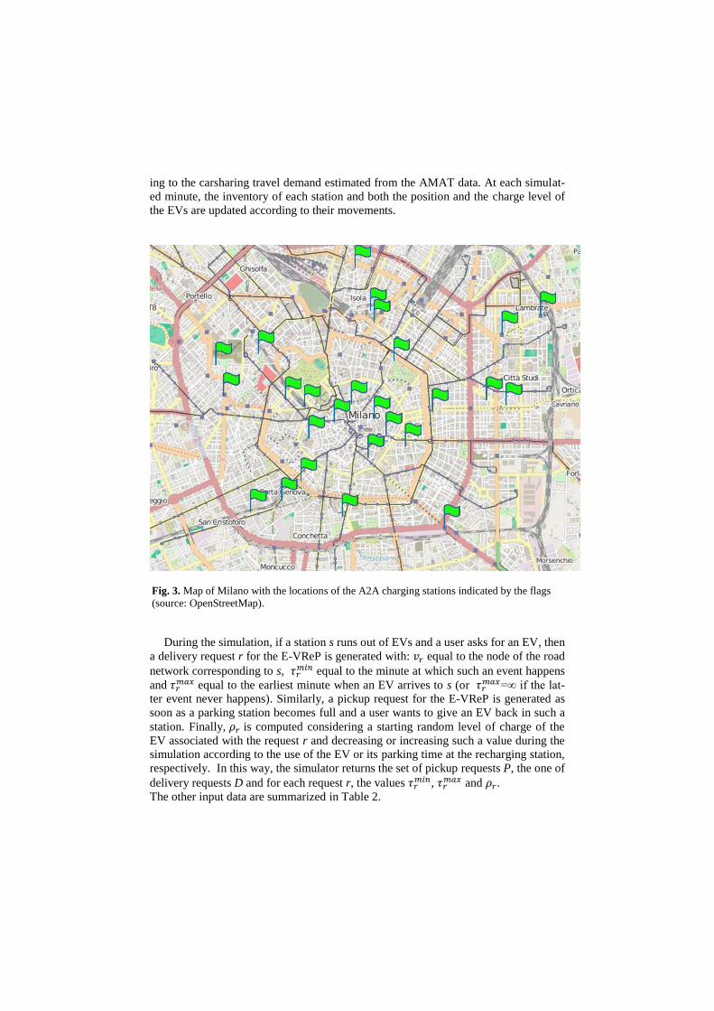
Fig. 3 shows the location of the A2A charging stations (i.e., 5 stations with 4 slots and

21 with 2 slots). The AMAT O-D zones have been intersected with a circular bounda-

ry of 500 meters around each charging station, representing the area easily reachable

by walking from the station. The intersection allows estimating the potential number

of movements that could be carried out with carsharing service rather than with pri-

vate car. Moreover, such values have been multiplied by 0.5% in order to consider

only a real-like percentage of the potential demand. Such a percentage is consistent

with the current usage of the Milano carsharing service.

With the aim of estimating the requests of the relocation staff, Bruglieri et al. 2014(b)

evaluated the unbalances due to the estimated carsharing travel demand through a

simulator. Such a carsharing simulator, developed in Matlab, has a time-step feed

with the data about the station capacities, the travel times between pairs of stations,

and the travel demands. More specifically, the simulator randomly generates the vehi-

cle movements between pairs of stations following a probability distribution accord-

ing to the carsharing travel demand estimated from the AMAT data. At each simulat-

ed minute, the inventory of each station and both the position and the charge level of

the EVs are updated according to their movements.

During the simulation, if a station s runs out of EVs and a user asks for an EV, then

a delivery request r for the E-VReP is generated with: 𝑣𝑟 equal to the node of the road

network corresponding to s, 𝜏𝑟𝑚𝑖𝑛 equal to the minute at which such an event happens

and 𝜏𝑟𝑚𝑎𝑥 equal to the earliest minute when an EV arrives to s (or 𝜏𝑟

𝑚𝑎𝑥=∞ if the lat-

ter event never happens). Similarly, a pickup request for the E-VReP is generated as

soon as a parking station becomes full and a user wants to give an EV back in such a

station. Finally, 𝜌𝑟 is computed considering a starting random level of charge of the

EV associated with the request r and decreasing or increasing such a value during the

simulation according to the use of the EV or its parking time at the recharging station,

respectively. In this way, the simulator returns the set of pickup requests P, the one of

delivery requests D and for each request r, the values 𝜏𝑟𝑚𝑖𝑛, 𝜏𝑟

𝑚𝑎𝑥 and 𝜌𝑟.

The other input data are summarized in Table 2.

Fig. 3. Map of Milano with the locations of the A2A charging stations indicated by the flags

(source: OpenStreetMap).

17

Input data Value

T 300 minutes

𝑠′ 25 km/h

𝑠′′ 15 km/h

𝑞’ 1 minute

𝑞’’ 1 minute

L 150 km

240 minutes

C 60€

Table 1. Values of the main input data

Concerning the AMAT set of instances, the testing phase has been carried out con-

sidering two different scenarios. In the former, the worker cost is not taken into ac-

count during the optimization process and therefore, the objective is only to maximize

the total number of relocation requests satisfied. While, in the latter, the aim is to

maximize the total profit as the difference between the total revenue associated with

the relocation requests satisfied and the total worker cost. In this latter scenario, the

worker cost is evaluated multiplying the number of the routes by the unitary personnel

cost, i.e., 60 €. The unitary personnel cost has been derived considering a time cost of

12 €/h (as in Boyaci et al., 2013), and that each operator is employed for a duty time

of 5 h. While the parameter revr (i.e. the revenue associated with the generic request r

satisfied) has been set to 20 € like the penalty cost for lost customers indicated in the

above cited paper.

Instead, the V-AMAT set of instances are characterized by a variable revenue as-

sociated with each relocation request. More specifically, 𝑟𝑒𝑣𝑟 , for each relocation

request r, is made up by two components. The first one represents a variable revenue

component (hereafter indicated with VRC), proportional to the actual rent-time of the

user that in the simulator generates the request r, by a factor equal to 0.29 €/minute.

While, the second one is a fixed revenue component (indicated by FRC) associated

with the customer satisfaction, i.e., it takes into account that a satisfied customer may

require the carsharing service also in the future. This second component, set to 15 €,

avoids that the relocation requests associated with customers requiring the carsharing

service only for a short rent-time are never satisfied. The value of 15 € arises from the

fact that we want to obtain profits comparable to those of AMAT set being the VRC

between 1.45 € and 4.35 € since the rent-times of the users are between 5 and 15

minutes.

The next two subsections will show the numerical results. In particular, with refer-

ence to the AMAT set, the comparisons between the solutions found by the proposed

heuristics and the two MILP formulations will be shown in Subsection 5.1. Moreover,

MILP1 and MILP2 will be also compared. While, concerning to the V-AMAT set, the

comparisons between the solutions found by the proposed heuristics and the MILP2

are given in Subsection 5.2.

Such comparisons will be discussed not only with reference to the quality of the

solution but also regarding the computational times.

5.1 Numerical results on the AMAT set

In this section, the experiments carried out on the benchmark instances are de-

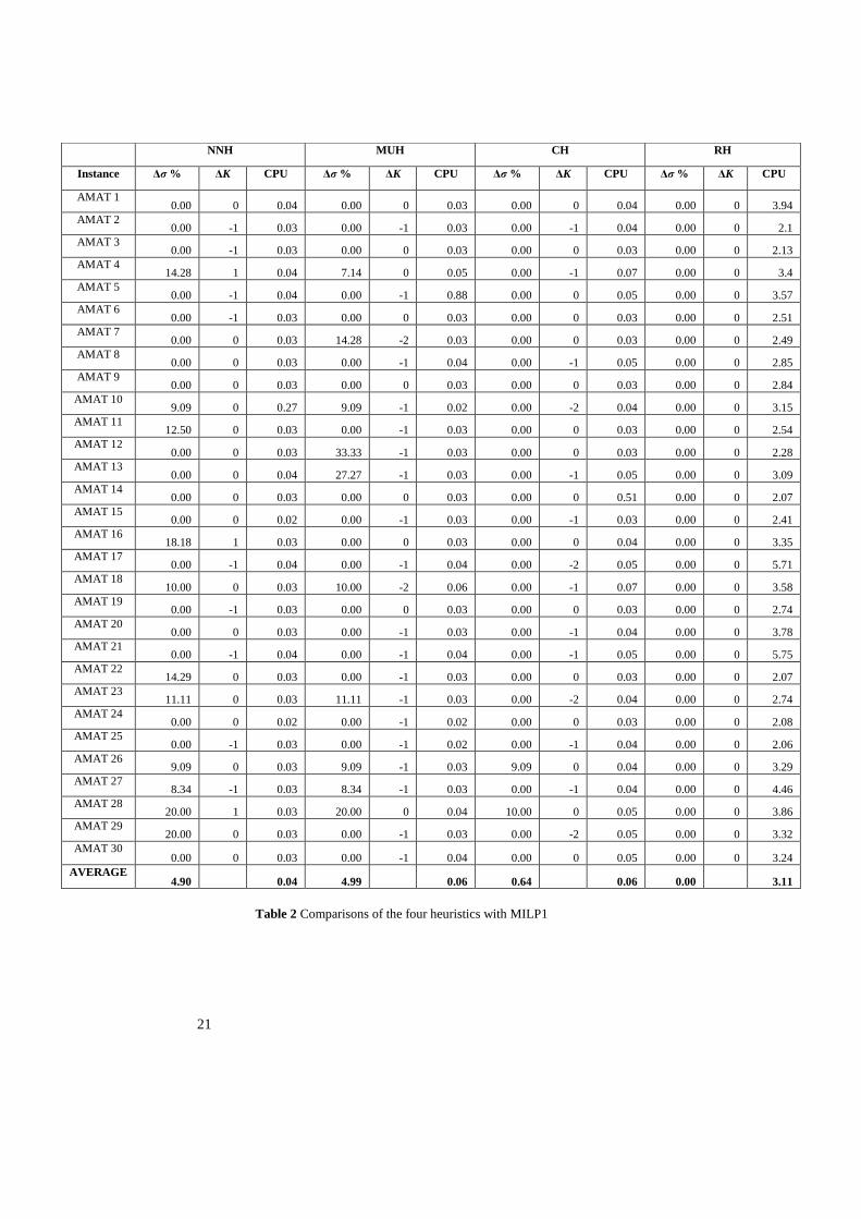
scribed and discussed. Table 3 compares the numerical results obtained by the four

heuristic approaches described in Section 3 and Section 4 with the ones reached solv-

ing MILP1. The header Δσ represents the percentage gaps on the number of served

requests found by MILP1 (𝜎𝑀𝐼𝐿𝑃1) and the heuristics (𝜎𝐻𝑒𝑢𝑟), computed as in the

following: 1

1100

MILP Heur

MILP

.

The header ΔK represents the gap between the number of workers employed by the

heuristics (𝐾𝐻𝑒𝑢𝑟) and the one employed by the MILP (𝐾𝑀𝐼𝐿𝑃1), evaluated as in the

following:

1 .MILP HeurK K K

The header CPU refers to the computational times required by a heuristic for solv-

ing each instance. The structured heuristics yield by far better results than the two

greedy ones.

The NNH and MUH do not obtain the optimal solution for eleven instances (with

an average Δσ gap equal to 12.33%) and for ten instances (with an average Δσ gap

equal to 14.97%), respectively; the CH, only for two instances (with an average Δσ

gap equal to 9.54%) and remarkably, the RH always detects the optimum.

As the number of the operators employed is concerned, the NNH uses for nine in-

stances one more worker than the optimal solution while in three instances, one less;

in the all other instances, it uses the same number of workers (hereafter, in the paper,

it is omitted to indicate the number of instances for which ΔK=0). Moreover, the only

three cases with a positive ΔK (i.e., AMAT 4, AMAT 16 and AMAT 28) are due to

the more requests handled by MILP1 than NNH, requiring one more worker.

The MUH, in nineteen instances, uses one more worker than the optimal solution

while in two instances, two more. The CH, in ten instances uses one more worker

while in four instances, two more and, remarkably, the RH always uses the same

number of workers employed in the optimum. RH is suitable to outperform the other

heuristics since it generates several feasible solutions and returns the best among

them. While, the other heuristics only generate one feasible solution.

Concerning the total computational times, the NNH gives the final solution in 0.04

s, on average, the MUH in 0.06 s, the CH in 0.06 s, and finally, the RH in 3.11 s,

against 24.34 s required by the MILP1.

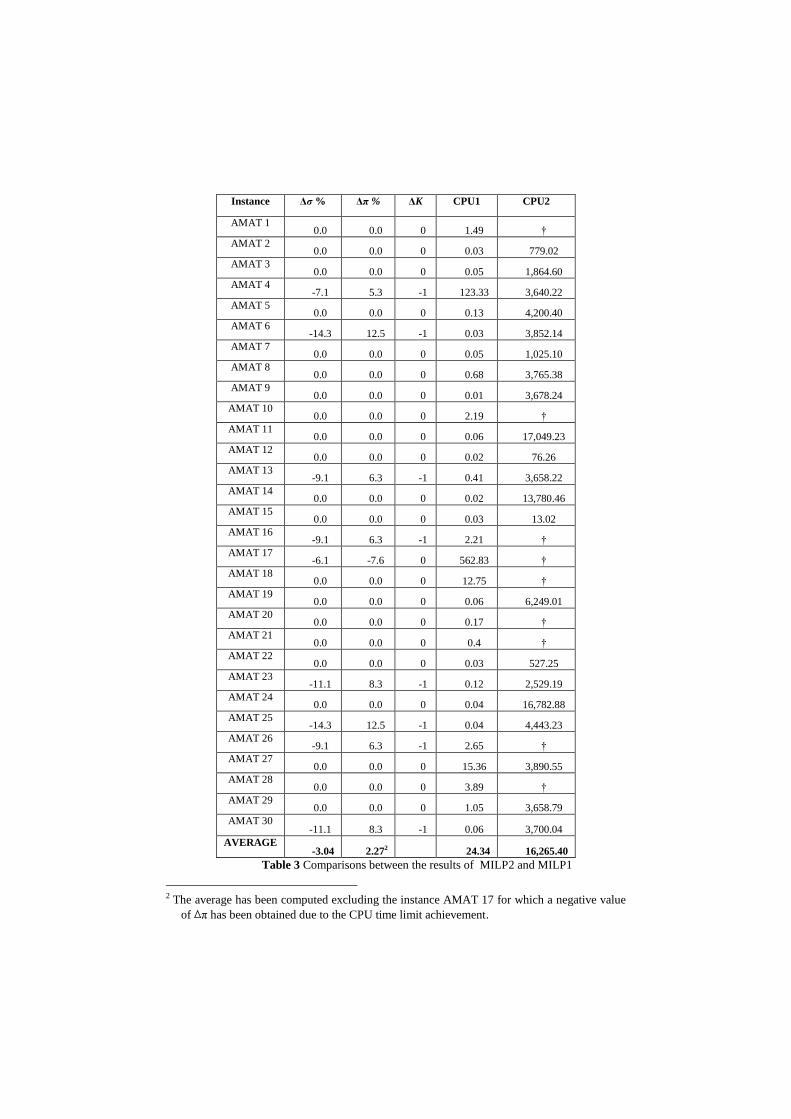
In Table 4, the results obtained considering the E-VReP with the new objective

function, introduced in Section 2, and the ones of MILP1 are compared. The header

Δσ denotes the percentage gap between the number of served requests by the E-VReP

with the new objective function and the original one. The header Δπ represents the

percentage gap between the total profit obtained by the new objective function and the

original one, as specified in the following: MILP 2 MILP1

MILP1100.

19

Finally, the header CPU1 and CPU2 show the computational times required by

MILP1 and MILP2, respectively.

On eight instances, MILP2 maximizes the total profit compared to MILP1 of 6.5%

on average although it decreases the number of served requests of 10.1% on average.

Since in MILP2, it could be not convenient (from the profit point of view) to serve the

same number of requests handled by MILP1. Moreover, a positive value of Δπ and a

negative value of ΔK always correspond to every negative value of Δσ.

Moreover, it is worth observing that the change applied to the objective function in

MILP2 decreases the computational performances since for twenty-three instances

the CPU time limit is reached requiring 16,265.4 s on average, against 24.30 s used by

MILP1.

In particular, in eight cases, MILP1 handles more requests than MILP2 but using

one worker more. Therefore, MILP2 guarantees a higher profit. There is only one

case (AMAT 17) in which MILP1 is able to handle more requests than MILP2, using

one less worker and then, guaranteeing a higher profit. However, this is a case in

which MILP2 reaches the CPU time limit.

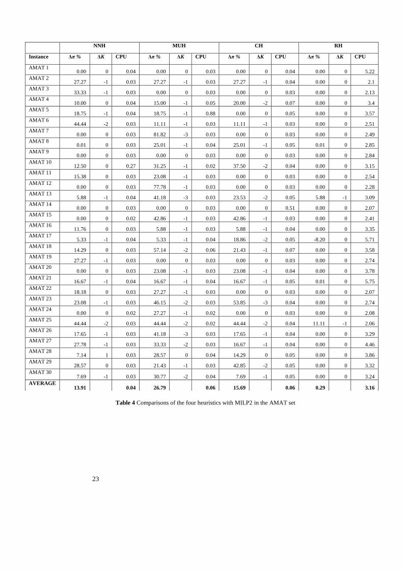
Table 5 compares the total profit obtained by the heuristics to the one of MILP2. In

particular: 2

MILP 2100

MILP Heur

and

2 .MILP HeurK K K

The NNH on average decreases the total profit of 18.97% compared to MILP2

while it uses in eleven instances one more worker and, in two instances, two more.

The MUH on average decreases the total profit of 32.14% compared to MILP2 while

it employs in sixteen instances one more worker, in five instances, two more and fi-

nally, in three instances, three more. The CH on average decreases the total profit of

24.77% with respect to MILP2 while it uses, in eleven instances, one more worker, in

six instances, two more and in one instance, three more. Finally, the RH on average

decreases the total profit only of 1.76% while it uses, only in two instances, one more

worker than MILP2.

Concerning the computational times, the NNH on average requires 0.04 s, the

MUH 0.06 s, the CH 0.06 s and finally, the RH 3.16 s, against 16,265.4 s of MILP2.

5.2 Numerical results on the V-AMAT set

In this subsection, the comparisons between the solutions found by the four pro-

posed heuristics and the ones found by the MILP2, on the V-AMAT set, are dis-

cussed.

Table 6 compares the total profit obtained by the heuristics to the one of MILP2.

The meaning of each column is the same of those of Table 5. The NNH on average

decreases the total profit of 16.77% compared to MILP2 while it uses in eight in-

stances one more worker. The MUH on average decreases the total profit of 24.74%

compared to MILP2 while it employs in six instances one less worker and in five

instances, one more worker. The CH on average decreases the total profit of 30.99%

with respect to MILP2 while it uses, in five instances, one fewer worker; in five in-

stances, one more worker; in one instance, two more workers and in one instance,

three more workers. Finally, the RH on average decreases the total profit only of

0.61% and only in one instance, it uses one more worker of the MILP2.

Concerning the computational times, the NNH on average requires 0.01 s as well

as the MUH while the CH, 0.02 s and finally, the RH 8.36 s, against 8,267.66 s of

MILP2.

21

NNH MUH CH RH

Instance Δσ % ΔK CPU Δσ % ΔK CPU Δσ % ΔK CPU Δσ % ΔK CPU

AMAT 1 0.00 0 0.04 0.00 0 0.03 0.00 0 0.04 0.00 0 3.94

AMAT 2 0.00 -1 0.03 0.00 -1 0.03 0.00 -1 0.04 0.00 0 2.1

AMAT 3 0.00 -1 0.03 0.00 0 0.03 0.00 0 0.03 0.00 0 2.13

AMAT 4 14.28 1 0.04 7.14 0 0.05 0.00 -1 0.07 0.00 0 3.4

AMAT 5 0.00 -1 0.04 0.00 -1 0.88 0.00 0 0.05 0.00 0 3.57

AMAT 6 0.00 -1 0.03 0.00 0 0.03 0.00 0 0.03 0.00 0 2.51

AMAT 7 0.00 0 0.03 14.28 -2 0.03 0.00 0 0.03 0.00 0 2.49

AMAT 8 0.00 0 0.03 0.00 -1 0.04 0.00 -1 0.05 0.00 0 2.85

AMAT 9 0.00 0 0.03 0.00 0 0.03 0.00 0 0.03 0.00 0 2.84

AMAT 10 9.09 0 0.27 9.09 -1 0.02 0.00 -2 0.04 0.00 0 3.15

AMAT 11 12.50 0 0.03 0.00 -1 0.03 0.00 0 0.03 0.00 0 2.54

AMAT 12 0.00 0 0.03 33.33 -1 0.03 0.00 0 0.03 0.00 0 2.28

AMAT 13 0.00 0 0.04 27.27 -1 0.03 0.00 -1 0.05 0.00 0 3.09

AMAT 14 0.00 0 0.03 0.00 0 0.03 0.00 0 0.51 0.00 0 2.07

AMAT 15 0.00 0 0.02 0.00 -1 0.03 0.00 -1 0.03 0.00 0 2.41

AMAT 16 18.18 1 0.03 0.00 0 0.03 0.00 0 0.04 0.00 0 3.35

AMAT 17 0.00 -1 0.04 0.00 -1 0.04 0.00 -2 0.05 0.00 0 5.71

AMAT 18 10.00 0 0.03 10.00 -2 0.06 0.00 -1 0.07 0.00 0 3.58

AMAT 19 0.00 -1 0.03 0.00 0 0.03 0.00 0 0.03 0.00 0 2.74

AMAT 20 0.00 0 0.03 0.00 -1 0.03 0.00 -1 0.04 0.00 0 3.78

AMAT 21 0.00 -1 0.04 0.00 -1 0.04 0.00 -1 0.05 0.00 0 5.75

AMAT 22 14.29 0 0.03 0.00 -1 0.03 0.00 0 0.03 0.00 0 2.07

AMAT 23 11.11 0 0.03 11.11 -1 0.03 0.00 -2 0.04 0.00 0 2.74

AMAT 24 0.00 0 0.02 0.00 -1 0.02 0.00 0 0.03 0.00 0 2.08

AMAT 25 0.00 -1 0.03 0.00 -1 0.02 0.00 -1 0.04 0.00 0 2.06

AMAT 26 9.09 0 0.03 9.09 -1 0.03 9.09 0 0.04 0.00 0 3.29

AMAT 27 8.34 -1 0.03 8.34 -1 0.03 0.00 -1 0.04 0.00 0 4.46

AMAT 28 20.00 1 0.03 20.00 0 0.04 10.00 0 0.05 0.00 0 3.86

AMAT 29 20.00 0 0.03 0.00 -1 0.03 0.00 -2 0.05 0.00 0 3.32

AMAT 30 0.00 0 0.03 0.00 -1 0.04 0.00 0 0.05 0.00 0 3.24

AVERAGE 4.90 0.04 4.99 0.06 0.64 0.06 0.00 3.11

Table 2 Comparisons of the four heuristics with MILP1

Instance Δσ % Δπ % ΔK CPU1 CPU2

AMAT 1 0.0 0.0 0 1.49 †

AMAT 2 0.0 0.0 0 0.03 779.02

AMAT 3 0.0 0.0 0 0.05 1,864.60

AMAT 4 -7.1 5.3 -1 123.33 3,640.22

AMAT 5 0.0 0.0 0 0.13 4,200.40

AMAT 6 -14.3 12.5 -1 0.03 3,852.14

AMAT 7 0.0 0.0 0 0.05 1,025.10

AMAT 8 0.0 0.0 0 0.68 3,765.38

AMAT 9 0.0 0.0 0 0.01 3,678.24

AMAT 10 0.0 0.0 0 2.19 †

AMAT 11 0.0 0.0 0 0.06 17,049.23

AMAT 12 0.0 0.0 0 0.02 76.26

AMAT 13 -9.1 6.3 -1 0.41 3,658.22

AMAT 14 0.0 0.0 0 0.02 13,780.46

AMAT 15 0.0 0.0 0 0.03 13.02

AMAT 16 -9.1 6.3 -1 2.21 †

AMAT 17 -6.1 -7.6 0 562.83 †

AMAT 18 0.0 0.0 0 12.75 †

AMAT 19 0.0 0.0 0 0.06 6,249.01

AMAT 20 0.0 0.0 0 0.17 †

AMAT 21 0.0 0.0 0 0.4 †

AMAT 22 0.0 0.0 0 0.03 527.25

AMAT 23 -11.1 8.3 -1 0.12 2,529.19

AMAT 24 0.0 0.0 0 0.04 16,782.88

AMAT 25 -14.3 12.5 -1 0.04 4,443.23

AMAT 26 -9.1 6.3 -1 2.65 †

AMAT 27 0.0 0.0 0 15.36 3,890.55

AMAT 28 0.0 0.0 0 3.89 †

AMAT 29 0.0 0.0 0 1.05 3,658.79

AMAT 30 -11.1 8.3 -1 0.06 3,700.04

AVERAGE -3.04 2.272 24.34 16,265.40

Table 3 Comparisons between the results of MILP2 and MILP1

2 The average has been computed excluding the instance AMAT 17 for which a negative value

of ∆π has been obtained due to the CPU time limit achievement.

23

Table 4 Comparisons of the four heuristics with MILP2 in the AMAT set

NNH MUH CH RH

Instance Δπ % ΔK CPU Δπ % ΔK CPU Δπ % ΔK CPU Δπ % ΔK CPU

AMAT 1 0.00 0 0.04 0.00 0 0.03 0.00 0 0.04 0.00 0 5.22

AMAT 2 27.27 -1 0.03 27.27 -1 0.03 27.27 -1 0.04 0.00 0 2.1

AMAT 3 33.33 -1 0.03 0.00 0 0.03 0.00 0 0.03 0.00 0 2.13

AMAT 4 10.00 0 0.04 15.00 -1 0.05 20.00 -2 0.07 0.00 0 3.4

AMAT 5 18.75 -1 0.04 18.75 -1 0.88 0.00 0 0.05 0.00 0 3.57

AMAT 6 44.44 -2 0.03 11.11 -1 0.03 11.11 -1 0.03 0.00 0 2.51

AMAT 7 0.00 0 0.03 81.82 -3 0.03 0.00 0 0.03 0.00 0 2.49

AMAT 8 0.01 0 0.03 25.01 -1 0.04 25.01 -1 0.05 0.01 0 2.85

AMAT 9 0.00 0 0.03 0.00 0 0.03 0.00 0 0.03 0.00 0 2.84

AMAT 10 12.50 0 0.27 31.25 -1 0.02 37.50 -2 0.04 0.00 0 3.15

AMAT 11 15.38 0 0.03 23.08 -1 0.03 0.00 0 0.03 0.00 0 2.54

AMAT 12 0.00 0 0.03 77.78 -1 0.03 0.00 0 0.03 0.00 0 2.28

AMAT 13 5.88 -1 0.04 41.18 -3 0.03 23.53 -2 0.05 5.88 -1 3.09

AMAT 14 0.00 0 0.03 0.00 0 0.03 0.00 0 0.51 0.00 0 2.07

AMAT 15 0.00 0 0.02 42.86 -1 0.03 42.86 -1 0.03 0.00 0 2.41

AMAT 16 11.76 0 0.03 5.88 -1 0.03 5.88 -1 0.04 0.00 0 3.35

AMAT 17 5.33 -1 0.04 5.33 -1 0.04 18.86 -2 0.05 -8.20 0 5.71

AMAT 18 14.29 0 0.03 57.14 -2 0.06 21.43 -1 0.07 0.00 0 3.58

AMAT 19 27.27 -1 0.03 0.00 0 0.03 0.00 0 0.03 0.00 0 2.74

AMAT 20 0.00 0 0.03 23.08 -1 0.03 23.08 -1 0.04 0.00 0 3.78

AMAT 21 16.67 -1 0.04 16.67 -1 0.04 16.67 -1 0.05 0.01 0 5.75

AMAT 22 18.18 0 0.03 27.27 -1 0.03 0.00 0 0.03 0.00 0 2.07

AMAT 23 23.08 -1 0.03 46.15 -2 0.03 53.85 -3 0.04 0.00 0 2.74

AMAT 24 0.00 0 0.02 27.27 -1 0.02 0.00 0 0.03 0.00 0 2.08

AMAT 25 44.44 -2 0.03 44.44 -2 0.02 44.44 -2 0.04 11.11 -1 2.06

AMAT 26 17.65 -1 0.03 41.18 -3 0.03 17.65 -1 0.04 0.00 0 3.29

AMAT 27 27.78 -1 0.03 33.33 -2 0.03 16.67 -1 0.04 0.00 0 4.46

AMAT 28 7.14 1 0.03 28.57 0 0.04 14.29 0 0.05 0.00 0 3.86

AMAT 29 28.57 0 0.03 21.43 -1 0.03 42.85 -2 0.05 0.00 0 3.32

AMAT 30 7.69 -1 0.03 30.77 -2 0.04 7.69 -1 0.05 0.00 0 3.24

AVERAGE 13.91 0.04 26.79 0.06 15.69 0.06 0.29 3.16

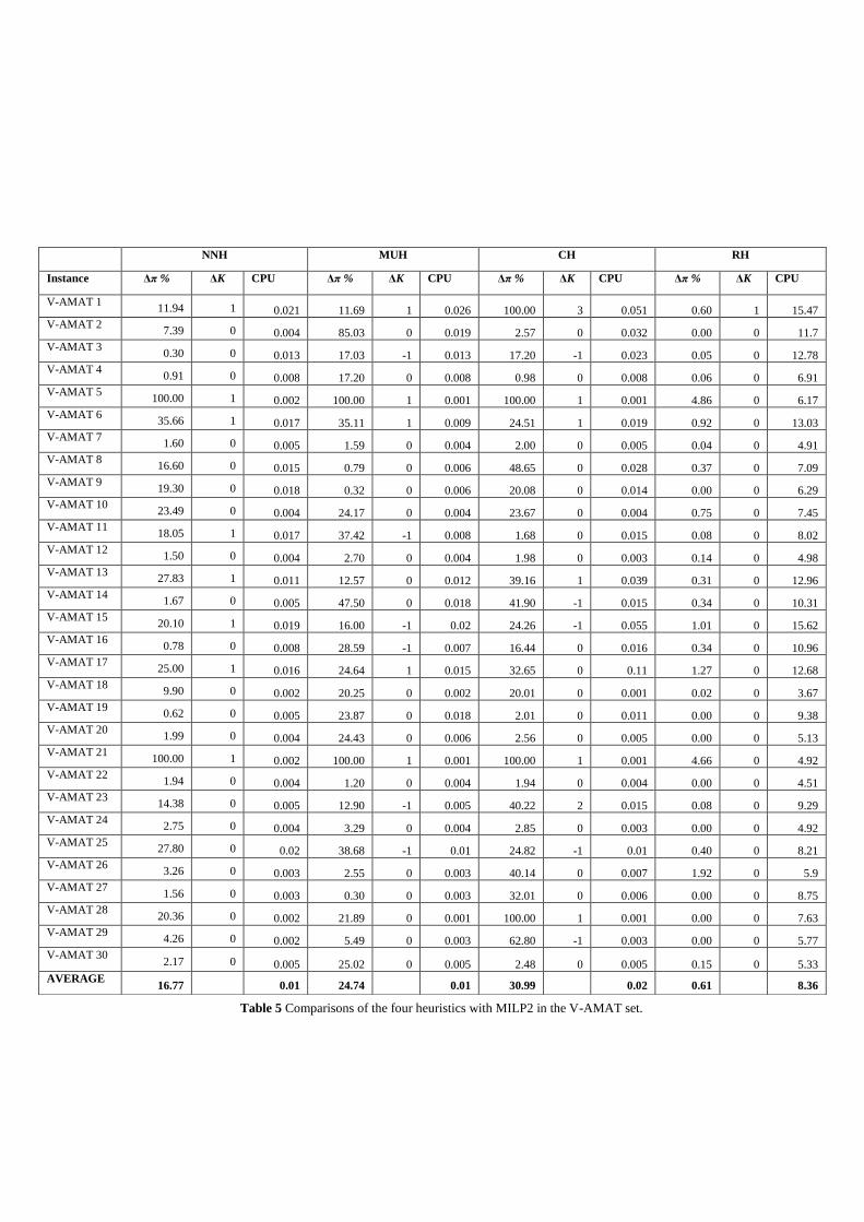
NNH MUH CH RH

Instance Δπ % ΔK CPU Δπ % ΔK CPU Δπ % ΔK CPU Δπ % ΔK CPU

V-AMAT 1 11.94 1 0.021 11.69 1 0.026 100.00 3 0.051 0.60 1 15.47

V-AMAT 2 7.39 0 0.004 85.03 0 0.019 2.57 0 0.032 0.00 0 11.7

V-AMAT 3 0.30 0 0.013 17.03 -1 0.013 17.20 -1 0.023 0.05 0 12.78

V-AMAT 4 0.91 0 0.008 17.20 0 0.008 0.98 0 0.008 0.06 0 6.91

V-AMAT 5 100.00 1 0.002 100.00 1 0.001 100.00 1 0.001 4.86 0 6.17

V-AMAT 6 35.66 1 0.017 35.11 1 0.009 24.51 1 0.019 0.92 0 13.03

V-AMAT 7 1.60 0 0.005 1.59 0 0.004 2.00 0 0.005 0.04 0 4.91

V-AMAT 8 16.60 0 0.015 0.79 0 0.006 48.65 0 0.028 0.37 0 7.09

V-AMAT 9 19.30 0 0.018 0.32 0 0.006 20.08 0 0.014 0.00 0 6.29

V-AMAT 10 23.49 0 0.004 24.17 0 0.004 23.67 0 0.004 0.75 0 7.45

V-AMAT 11 18.05 1 0.017 37.42 -1 0.008 1.68 0 0.015 0.08 0 8.02

V-AMAT 12 1.50 0 0.004 2.70 0 0.004 1.98 0 0.003 0.14 0 4.98

V-AMAT 13 27.83 1 0.011 12.57 0 0.012 39.16 1 0.039 0.31 0 12.96

V-AMAT 14 1.67 0 0.005 47.50 0 0.018 41.90 -1 0.015 0.34 0 10.31

V-AMAT 15 20.10 1 0.019 16.00 -1 0.02 24.26 -1 0.055 1.01 0 15.62

V-AMAT 16 0.78 0 0.008 28.59 -1 0.007 16.44 0 0.016 0.34 0 10.96

V-AMAT 17 25.00 1 0.016 24.64 1 0.015 32.65 0 0.11 1.27 0 12.68

V-AMAT 18 9.90 0 0.002 20.25 0 0.002 20.01 0 0.001 0.02 0 3.67

V-AMAT 19 0.62 0 0.005 23.87 0 0.018 2.01 0 0.011 0.00 0 9.38

V-AMAT 20 1.99 0 0.004 24.43 0 0.006 2.56 0 0.005 0.00 0 5.13

V-AMAT 21 100.00 1 0.002 100.00 1 0.001 100.00 1 0.001 4.66 0 4.92

V-AMAT 22 1.94 0 0.004 1.20 0 0.004 1.94 0 0.004 0.00 0 4.51

V-AMAT 23 14.38 0 0.005 12.90 -1 0.005 40.22 2 0.015 0.08 0 9.29

V-AMAT 24 2.75 0 0.004 3.29 0 0.004 2.85 0 0.003 0.00 0 4.92

V-AMAT 25 27.80 0 0.02 38.68 -1 0.01 24.82 -1 0.01 0.40 0 8.21

V-AMAT 26 3.26 0 0.003 2.55 0 0.003 40.14 0 0.007 1.92 0 5.9

V-AMAT 27 1.56 0 0.003 0.30 0 0.003 32.01 0 0.006 0.00 0 8.75

V-AMAT 28 20.36 0 0.002 21.89 0 0.001 100.00 1 0.001 0.00 0 7.63

V-AMAT 29 4.26 0 0.002 5.49 0 0.003 62.80 -1 0.003 0.00 0 5.77

V-AMAT 30 2.17 0 0.005 25.02 0 0.005 2.48 0 0.005 0.15 0 5.33

AVERAGE 16.77 0.01 24.74 0.01 30.99 0.02 0.61 8.36

Table 5 Comparisons of the four heuristics with MILP2 in the V-AMAT set.

25

6 Sensitivity analysis

In this section, we perform a sensitivity analysis on the main input parameters of

the E-VReP, such as the number of relocation requests (instance size) and the revenue

associated with each of them.

6.1 Sensitivity analysis on the instance size

The sensitivity analysis on the instance size has been carried out considering the

results obtained by the exact model MILP2 on both the AMAT and V-AMAT set. The

results have been analyzed from the point of view of the profit, of the percentage

number of requests served and of the number of operators used.

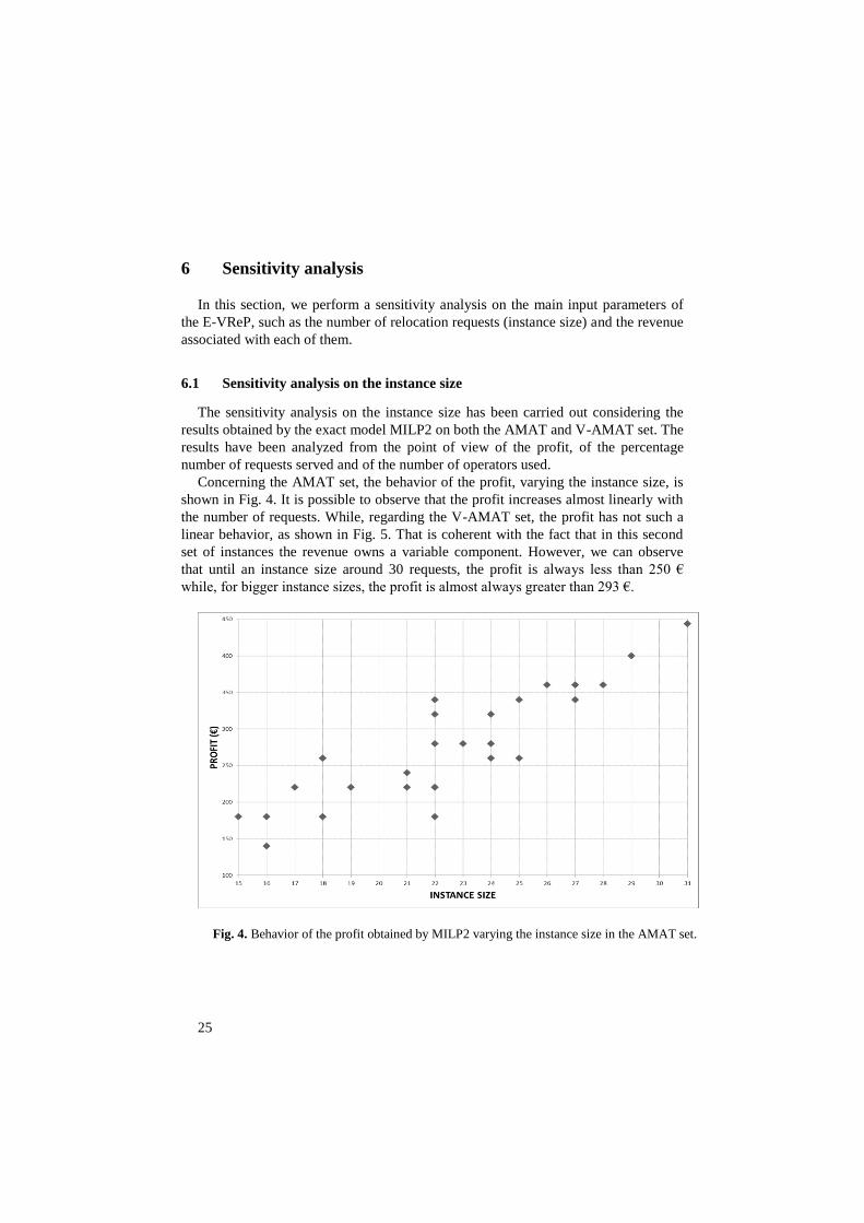
Concerning the AMAT set, the behavior of the profit, varying the instance size, is

shown in Fig. 4. It is possible to observe that the profit increases almost linearly with

the number of requests. While, regarding the V-AMAT set, the profit has not such a

linear behavior, as shown in Fig. 5. That is coherent with the fact that in this second

set of instances the revenue owns a variable component. However, we can observe

that until an instance size around 30 requests, the profit is always less than 250 €

while, for bigger instance sizes, the profit is almost always greater than 293 €.

Fig. 4. Behavior of the profit obtained by MILP2 varying the instance size in the AMAT set.

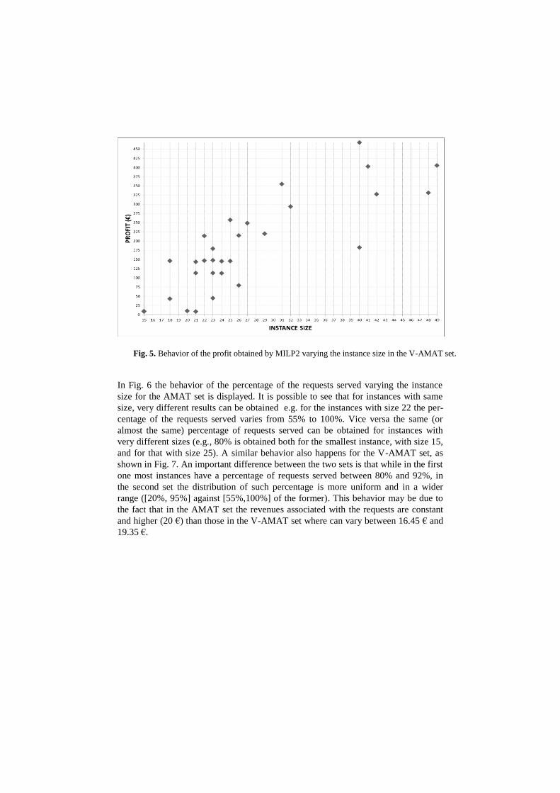
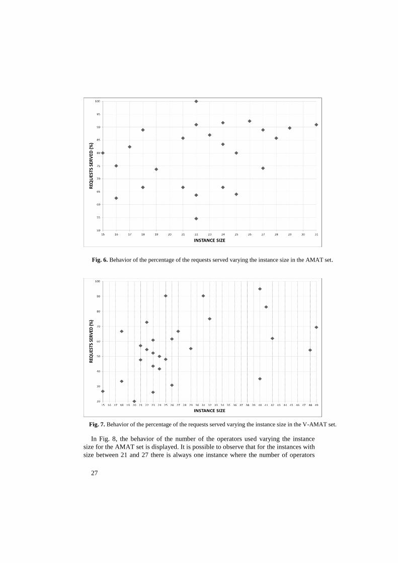
In Fig. 6 the behavior of the percentage of the requests served varying the instance

size for the AMAT set is displayed. It is possible to see that for instances with same

size, very different results can be obtained e.g. for the instances with size 22 the per-

centage of the requests served varies from 55% to 100%. Vice versa the same (or

almost the same) percentage of requests served can be obtained for instances with

very different sizes (e.g., 80% is obtained both for the smallest instance, with size 15,

and for that with size 25). A similar behavior also happens for the V-AMAT set, as

shown in Fig. 7. An important difference between the two sets is that while in the first

one most instances have a percentage of requests served between 80% and 92%, in

the second set the distribution of such percentage is more uniform and in a wider

range ([20%, 95%] against [55%,100%] of the former). This behavior may be due to

the fact that in the AMAT set the revenues associated with the requests are constant

and higher (20 €) than those in the V-AMAT set where can vary between 16.45 € and

19.35 €.

Fig. 5. Behavior of the profit obtained by MILP2 varying the instance size in the V-AMAT set.

27

In Fig. 8, the behavior of the number of the operators used varying the instance

size for the AMAT set is displayed. It is possible to observe that for the instances with

size between 21 and 27 there is always one instance where the number of operators

Fig. 6. Behavior of the percentage of the requests served varying the instance size in the AMAT set.

Fig. 7. Behavior of the percentage of the requests served varying the instance size in the V-AMAT set.

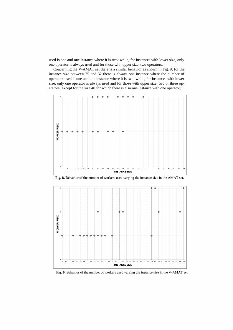
used is one and one instance where it is two; while, for instances with lower size, only

one operator is always used and for those with upper size, two operators.

Concerning the V-AMAT set there is a similar behavior as shown in Fig. 9: for the

instance size between 25 and 32 there is always one instance where the number of

operators used is one and one instance where it is two; while, for instances with lower

size, only one operator is always used and for those with upper size, two or three op-

erators (except for the size 40 for which there is also one instance with one operator).

Fig. 8. Behavior of the number of workers used varying the instance size in the AMAT set.

Fig. 9. Behavior of the number of workers used varying the instance size in the V-AMAT set.

29

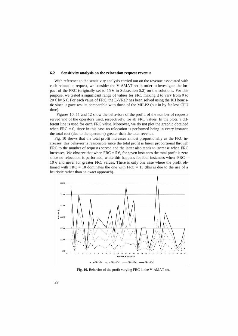
6.2 Sensitivity analysis on the relocation request revenue

With reference to the sensitivity analysis carried out on the revenue associated with

each relocation request, we consider the V-AMAT set in order to investigate the im-

pact of the FRC (originally set to 15 € in Subsection 5.2) on the solutions. For this

purpose, we tested a significant range of values for FRC making it to vary from 0 to

20 € by 5 €. For each value of FRC, the E-VReP has been solved using the RH heuris-

tic since it gave results comparable with those of the MILP2 (but in by far less CPU

time).

Figures 10, 11 and 12 show the behaviors of the profit, of the number of requests

served and of the operators used, respectively, for all FRC values. In the plots, a dif-

ferent line is used for each FRC value. Moreover, we do not plot the graphic obtained

when FRC = 0, since in this case no relocation is performed being in every instance

the total cost (due to the operators) greater than the total revenue.

Fig. 10 shows that the total profit increases almost proportionally as the FRC in-

creases: this behavior is reasonable since the total profit is linear proportional through

FRC to the number of requests served and the latter also tends to increase when FRC

increases. We observe that when FRC = 5 €, for seven instances the total profit is zero

since no relocation is performed, while this happens for four instances when FRC =

10 € and never for greater FRC values. There is only one case where the profit ob-

tained with FRC = 10 dominates the one with FRC = 15 (this is due to the use of a

heuristic rather than an exact approach).

Fig. 10. Behavior of the profit varying FRC in the V-AMAT set.

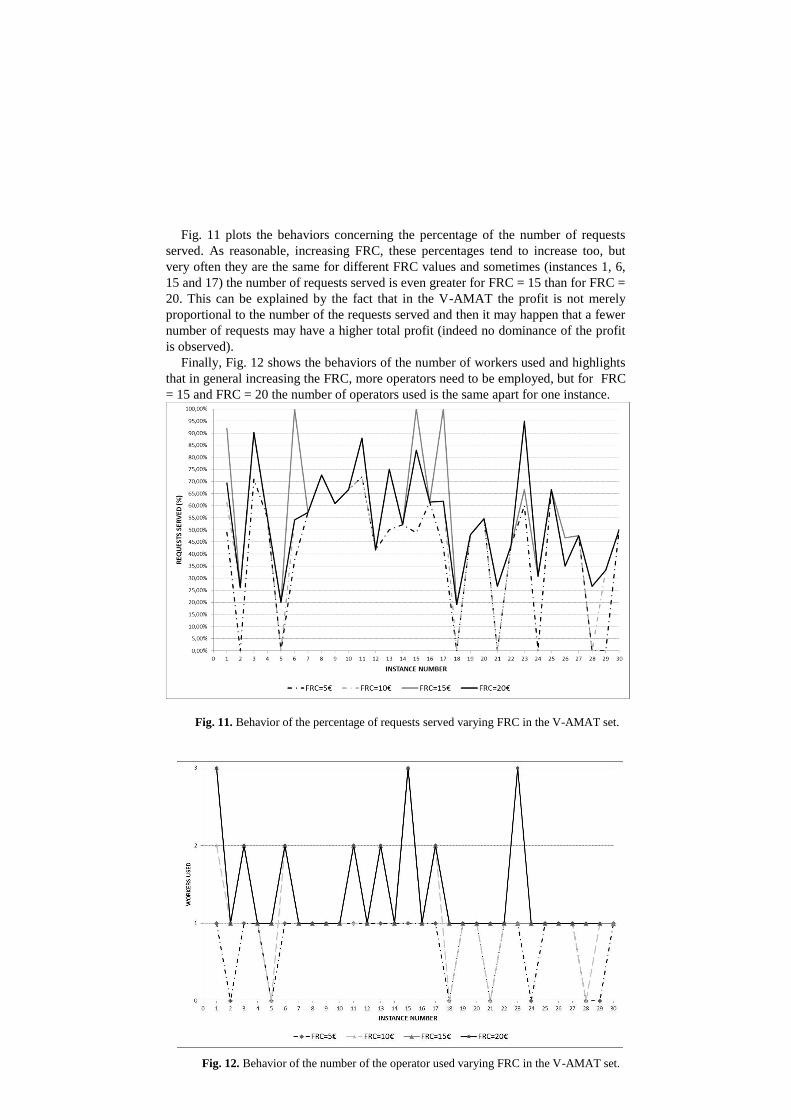
Fig. 11 plots the behaviors concerning the percentage of the number of requests

served. As reasonable, increasing FRC, these percentages tend to increase too, but

very often they are the same for different FRC values and sometimes (instances 1, 6,

15 and 17) the number of requests served is even greater for FRC = 15 than for FRC =

20. This can be explained by the fact that in the V-AMAT the profit is not merely

proportional to the number of the requests served and then it may happen that a fewer

number of requests may have a higher total profit (indeed no dominance of the profit

is observed).

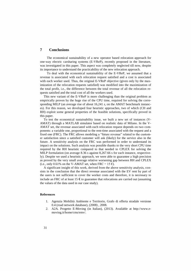
Finally, Fig. 12 shows the behaviors of the number of workers used and highlights

that in general increasing the FRC, more operators need to be employed, but for FRC

= 15 and FRC = 20 the number of operators used is the same apart for one instance.

Fig. 11. Behavior of the percentage of requests served varying FRC in the V-AMAT set.

Fig. 12. Behavior of the number of the operator used varying FRC in the V-AMAT set.

31

7 Conclusions

The economical sustainability of a new operator based relocation approach for

one-way electric carsharing systems (E-VReP), recently proposed in the literature,

was investigated in this paper. This aspect was completely neglected till now, despite

its importance to understand the practicability of the new relocation approach.

To deal with the economical sustainability of the E-VReP, we assumed that a

revenue is associated with each relocation request satisfied and a cost is associated

with each worker used. Thus, the original E-VReP objective (given only by the max-

imization of the relocation requests satisfied) was modified into the maximization of

the total profit, i.e., the difference between the total revenue of all the relocation re-

quests satisfied and the total cost of all the workers used.

This new variant of the E-VReP is more challenging than the original problem as

empirically proven by the huge rise of the CPU time, required for solving the corre-

sponding MILP (an average rise of about 16,241 s, on the AMAT benchmark instanc-

es). For this reason, we developed four heuristic approaches, two of which (CH and

RH) exploit some general properties of the feasible solutions, specifically proved in

this paper.

To test the economical sustainability issue, we built a new set of instances (V-

AMAT) through a MATLAB simulator based on realistic data of Milano. In the V-

AMAT set, the revenue associated with each relocation request depends on two com-

ponents: a variable one, proportional to the rent-time associated with the request and a

fixed one (FRC). The FRC allows modeling a “future revenue” related to the custom-

er satisfaction since a satisfied customer will ask (likely) for the service also in the

future. A sensitivity analysis on the FRC was performed in order to understand its

impact on the solutions. Such analysis was possible thanks to the very short CPU time

required by the RH heuristic compared to that needed to CPLEX for solving the

MILP formulation (on average 8.36 s against 8,267.66 s for each instance, respective-

ly). Despite we used a heuristic approach, we were able to guarantee a high precision

as proved by the very small average relative worsening gap between RH and CPLEX

(i.e., only 0.61% on the V-AMAT set, when FRC = 15 €).

A significant insight of this work, derived from the above sensitivity analysis, con-

sists in the conclusion that the direct revenue associated with the EV rent by part of

the users is not sufficient to cover the worker costs and therefore, it is necessary to

include an FRC of at least 15 € to guarantee that relocations are carried out (assuming

the values of the data used in our case study).

References

1. Agenzia Mobilità Ambiente e Territorio, Grafo di offerta stradale versione

0.4 (road network database), (2008) , 2008.

2. A2A. Progetto E-Moving (in Italian), (2013). Available at http://www.e-

moving.it/home/cms/emv/.

3. AMAT. Dati sul traffico veicolare privato sulla rete stradale di Milano –

(Origin Destination Matrix, in Italian), (2005). Available at

http://www.amat-mi.it/it/downloads/8/.

4. Archetti, C., Speranza, M., 2004. Vehicle routing in the 1-skip collection

problem. Journal of the Operational Research Society 55 , no. 7, 717-727.

5. Aringhieri, R., Bruglieri, M., Malucelli, F., Nonato, M., 2004. An

asymmetric vehicle routing problem arising in the collection and disposal of

special waste. Electronic notes in discrete mathematics 17, 41-47.

6. Ahuja, R. K., Magnanti, T. L., Orlin, J. B., 1993. Network Flows: Theory,

Algorithms, and Applications. Prentice Hall.

7. Barth, M.,Todd, M., 1999. Simulation model performance analysis of a

multiple station shared vehicle system. Transportation Research Part C:

Emerging Technologies 7, no. 4, 237-259.

8. Barth, M., Todd, M., Xue, L., 2004. User-based vehicle relocation

techniques for multiple-station shared-use vehicle systems. Transportation

Research Record 1887, 137-144.

9. Boyacı, B., Geroliminis, N., Zografos, K., 2013. An optimization framework

for the development of efficient one-way car sharing systems. 13th Swiss

Transport Research conference.

10. Bruglieri, M., Colorni, A., Luè, A., 2014(a). The vehicle relocation problem

for the one-way electric vehicle sharing. Networks, 64(4), 292-305. (ArXive

pre-print version of the paper available at: http://arxiv.org/abs/1307.7195v1).

11. Bruglieri, M., Colorni, A., Luè, A., 2014(b). The vehicle relocation problem

for the one-way electric vehicle sharing: an application to the Milan case.

Procedia Social and Behavioral Sciences 111, 18-27.

12. Correia, G. H. A., Antunes, A. P., 2012. Optimization approach to depot

location and trip selection in one-way carsharing systems. Transportation

Research Part E: Logistics and Transportation Review 48, 233–247.

13. Correia, G. H. A., Jorge, D. R., Antunes, D. M., 2014. The Added Value of

Accounting For Users’ Flexibility and Information on the Potential of a

Station-Based One-Way Car-Sharing System: An Application in Lisbon,

Portugal. Journal of Intelligent Transportation Systems: Technology,

Planning, and Operations, 18(3), 299-308.

14. Cucu T., Ion, L., Ducq, Y. and Boussier, J.-M, 2009. Management of a

public transportation service: Carsharing service. Proceedings of The 6th

International Conference on Theory and Practice in Performance

Measurement and Management.

15. Di Febbraro, A., Sacco, N., Saeednia, M., 2012. One-way carsharing:

Solving the relocation problem. Transportation Research Board 91st Annual

Meeting.

16. Du, Y., Hall, R., 1997. Fleet sizing and empty equipment redistribution for

center-terminal transportation networks. Management Science 43, no. 2,

145-157.

17. European Commission, White paper: Roadmap to a single european

transport area–towards a competitive and resource efficient transport

system, (2011). COM (2011), vol. 144.

33

18. Fourer, R., Gay, D., Kernighan, B. W., 2002. The ampl book. Duxbury

Press, Pacific Grove.

19. Hafez, N., Parent, M., Proth, J. M., 2011. Managing a pool of self service

cars. Intelligent Transportation Systems. Proceedings. 2001 IEEE, IEEE,

943-948.

20. Jorge, D., Correia, G. H. A., 2013. Carsharing systems demand estimation

and defined operations: a literature review. European Journal of Transport

and Infrastructure Research, 13, 201-220.

21. Jung, J., Chow, J. Y., Jayakrishnan, R., & Park, J. Y., 2014. Stochastic

dynamic itinerary interception refueling location problem with queue delay

for electric taxi charging stations. Transportation Research Part C: Emerging

Technologies, 40, 123-142.

22. Kek, A. G., Cheu, R. L., Meng, Q., Fung, C. H., 2009. A decision support

system for vehicle relocation operations in carsharing systems.

Transportation Research Part E: Logistics and Transportation Review 45, no.

1, 149-158.

23. Nourinejad, M., Roorda, M. J., 2014. A dynamic carsharing decision support

system. Transportation Research Part E, 66, 36--50.

24. Touati-Moungla, N., Jost, V., 2012. Combinatorial optimization for electric

vehicles management. Journal of Energy and Power Engineering 6, no. 5,

738-743.

25. Wang, H., Cheu, R. , Lee, D. H., 2010. Logistical Inventory Approach in

Forecasting and Relocating Share-use Vehicles. Advanced Computer Con-

trol (ICACC), 2010 2nd International Conference on , 5, 314-318.