A branch and bound based heuristic for makespan

minimization of washing operations in hospital

sterilization services

Onur Ozturk, Mehmet A. Begen∗, Gregory S. Zaric

Ivey Business School, Western University, 1255 Western Road London Ontario, Canada

N6G 0N1

Abstract

In this paper, we address the problem of parallel batching of jobs on identicalmachines to minimize makespan. The problem is motivated from the washingstep of hospital sterilization services where jobs have different sizes, differentrelease dates and equal processing times. Machines can process more thanone job at the same time as long as the total size of jobs in a batch does notexceed the machine capacity. We present a branch and bound based heuristicmethod and compare it to a linear model and two other heuristics from theliterature. Computational experiments show that our method can find highquality solutions within short computation time.

Keywords: OR in health services, parallel batch scheduling, makespan,branch and bound heuristic

1. Introduction

Sterilization services are hospital departments where medical devices (MDs)are sterilized. There are two types of MDs: single use MDs and reusable MDs.Reusable MDs (RMDs) are used in surgeries, sterilized, and then reused inother surgeries. We consider the sterilization process of RMDs in this study.

∗corresponding author (tel: +1 519 661 4146 )Email addresses: oozturk@uwo.ca (Onur Ozturk), mbegen@ivey.uwo.ca (Mehmet

A. Begen), gzaric@ivey.uwo.ca (Gregory S. Zaric)

Preprint submitted to European Journal of Operational Research April 29, 2014

All RMDs used in a surgery constitute the RMD set of the surgery. Aftera surgery, all RMDs used are sent to the sterilization service. Due to surgerycharacteristics and surgeons needs, RMD sets may contain different numbersand types of instruments. Hence, they may have different sizes (or volumes).Moreover, they are sent to the sterilization service at different times withina day since each surgery may have a different starting and ending time.

A typical sterilization service is composed of the following steps (Di Mas-colo and Gouin (2013)): pre-disinfection, washing, packing and sterilization.Pre-disinfection is a manual step during which RMDs are submerged in achemical substance. Then, they are washed in an automatic washer. After-wards, they are packed and sterilized with steam in autoclaves.

We are interested in the washing step which is a bottleneck for steril-ization services. More than one RMD set can be washed in an automaticwasher at the same as long as the machine capacity is not exceeded. AllRMD sets washed at the same time constitute a single batch. Dependingon the organization between operating theatres and the sterilization service,RMD arrivals can be known in advance. For instance, RMD arrivals canbe known accurately for operating theatres where ambulatory surgeries takeplace. Another example is sterilization services that accept RMD arrivalsonly at specific times within a day. However, although RMD arrival timesand sizes are known in advance, the decision of how to load the machines,i.e., how to batch RMD sets and launch washing cycles is not trivial. Wemodel this problem using a parallel batch scheduling approach. Jobs mayhave different sizes (or volumes), different release dates and equal processingtimes. All jobs processed at the same time constitute a single batch which isprocessed on a single machine. The processing time of batches are the sameand equal to the processing time of jobs. Hence, our problem becomes a par-allel batching problem where RMD sets are treated as jobs having differentsizes, different release dates and equal processing times.

The remainder of this paper is organized as follows. In section 2, weprovide a literature review about batch scheduling problems and summarizethe contributions of this paper. In section 3, we give a formal descriptionof our problem. Section 4 is dedicated to the solution methodology. Section5 presents computational tests. Finally, we conclude the study and proposesome further research directions.

2

2. Literature review

2.1. Batch scheduling

We review only batch scheduling literature regarding jobs with differentsizes. For more information about batch scheduling, we refer the reader toPotts and Kovalyov (2000) and Mathirajan and Sivakumar (2006). There aretwo types of batch scheduling: serial and parallel. In serial batch scheduling,jobs in the same batch are processed sequentially on one or more machines.The processing of a batch is completed when the last job of the batch isprocessed. A typical example is confection workshops where many types ofclothes are sewed. For instance, sewing of t-shirts constitutes a batch whileshirts, trousers, etc. may constitute a second batch. In parallel batchinghowever, all jobs are processed simultaneously in the same machine. In thispaper, we study a parallel batch scheduling problem.

2.1.1. Exact methods

To the best of our knowledge, exact methods for parallel batching withjobs having different processing times are only applied to the case when alljobs are available at the same time. Uzsoy (1994) proposes a branch andbound algorithm to minimize the sum of job completion times on a singlemachine in which jobs have different processing times and sizes. For thesame problem but with the objective of minimizing makespan, Dupont andDhaenens-Flipo (2002) develop a branch and bound algorithm. Later on,Parsa et al. (2010) propose a branch and price method for the same problem.They report that their method is more efficient in terms of solution time thanthe one proposed by Dupont and Dhaenens-Flipo (2002). Malapert et al.(2012) study the minimization of maximum lateness on a single machine forwhich they propose a constraint programming approach. Other than thesestudies, there are many other studies where the case of unit size jobs istackled. For instance, Yuan et al. (2004) study the case where jobs have unitsizes but different processing times and release dates in the presence of jobfamilies. They provide dynamic programming algorithms when the numberof jobs, number of job families and number of release dates are bounded. Forthe general case, they propose a 2-approximation algorithm. Cheng et al.(2005) propose polynomial time dynamic programming algorithms for a setof regular objective functions when jobs have unit sizes, unit processing times,release dates and precedence constraints in the presence of a single machine.

3

Regardless of processing times, all problems considering different job sizesare in the class of NP-hard. The additional difficulty in our problem is dueto different release dates.

2.1.2. Heuristic and approximation methods

Most studies on batch scheduling with different job sizes focus on heuris-tic, meta-heuristic methods and approximation algorithms. Zhang et al.(2001) consider the case where jobs are available at the same time whilehaving different sizes and processing times. They develop an approximationalgorithm with a worst case performance ratio equal to 7/4 for makespanminimization on a single machine. Cheng et al. (2012) propose an approxi-mation algorithm with a worst case ratio of 2 and (8/3 - 2/3*m) for makespanand total completion time criteria, respectively, in the presence of m identicalmachines. Li et al. (2005) extend the problem studied in Zhang et al. (2001)by considering job release dates. They present a 2+ε approximation algo-rithm which is derived from a polynomial time approximation scheme thatthey propose for the case where jobs have unit sizes. Lu et al. (2010) use asimilar approach and provide a 2+ε approximation algorithm for bi-objectiveminimization of makespan and penalization of unscheduled jobs. Liu et al.(2014) present heuristics and approximation algorithms for makespan min-imization in the presence of unit size jobs with release dates and differentprocessing times. Their work is later generalized to the case of different jobsizes by Li (2012). Chou (2007) studies the same problem as in Li et al. (2005)and proposes a genetic algorithm using a dynamic programming procedureto find the makespan of a given chromosome.

Because in our problem we have release dates, different job sizes and par-allel machines, the articles cited in this paragraph are more related to ourproblem. Li (2012) presents the only approximation algorithm with a worstcase performance ratio equal to 2+ε when jobs have different sizes, differentprocessing times, release dates. There are, however, mostly heuristic/meta-heuristic methods in the literature for the batch scheduling problem studiedby Li (2012). For the same problem, Chung et al. (2009) propose a mixed in-teger linear programming model (MILP) and heuristics. Many other authorsuse the heuristics of Chung et al. (2009) for benchmarking. Wang and Chou(2010), Damodaran and Velez Gallego (2010) and Damodaran et al. (2011)consider the same problem for which they develop a genetic algorithm, agreedy randomized adaptive search procedure (GRASP) meta-heuristic anda constructive heuristic, respectively. All report that their approaches out-

4

perform the heuristics proposed in Chung et al. (2009). In another work,Damodaran and Velez-Gallego (2012) propose a simulated annealing algo-rithm which is able compete with the GRASP approach. Ozturk et al. (2012)develop a MILP model that runs faster than that proposed by Chung et al.(2009) for the case with equal job processing times. They also treat somespecial cases and provide optimal greedy algorithms. Recently, Pearn et al.(2013) enlarge the broad of the problem considering job families, due datesand set-up times between the processing of batches from different families.

2.2. Contribution of this paper

The method we propose exploits the structural properties of the problemunder study. It is based on constructing a search tree where each node rep-resents a job release date or the starting time of batch processing thanks toequal job processing time property. Numerical tests show that our branchbound based heuristic method (B&BH) can solve problem instances contain-ing up to 40 jobs in short computational time and can solve larger instancesin reasonable time. MILP model of Ozturk et al. (2012) can find the opti-mal solution for small and medium size instances but it requires too muchcomputational time. Regarding other methods from the literature, bench-marking results show that our method’s solution quality is higher than twoothers heuristics from the literature. Our method is applicable in sterilizationservices since it can quickly solve real size instances.

3. Problem description, notation and complexity

We begin with definitions and notation:

• There are m identical parallel machines with a limited capacity B.

• There are n jobs to be processed. A job is a task that is characterizedby a release date, rj, a size, wj, and a processing time, p.

• The size of a job cannot be greater than the machine capacity.

• Since washing times are the same for all RMD sets, job processing timesare the same for all jobs.

• A batch is composed of jobs processed at the same time on the samemachine. Several jobs can be batched together, complying with themachine capacity constraint.

5

• Once the processing of a batch is started, it cannot be interrupted (i.e.pre-emption is not allowed). Jobs cannot be split into multiple batches.

• The objective is to minimize makespan.

Using the Graham’s notation (Graham et al. (1979)), we have a P |p −batch, rj, pj = p, wj, B|Cmax scheduling problem. In this notation, P standsfor identical machines. p − batch indicates that we have a parallel batchingproblem where all jobs in the same batch are processed at the same time. rjand wj stands for job release dates and sizes, respectively. pj = p indicatesthat all job processing times are equal to p. B is the machine capacity.Finally, Cmax is the objective function.

It is straightforward to show that this problem is NP-hard. Consider thespecial case where all jobs are simultaneously available at instant 0 (1|p −batch, rj = 0, pj = p, wj, B|Cmax). Then, minimizing makespan is equivalentto minimizing the number of batches, which is a bin-packing problem. Sincebin-packing is strongly NP-hard, our problem is also strongly NP-hard.

4. Solution methodology

In this section, we present first a lower bound algorithm and then a branchand bound based heuristic for the problem of makespan minimization. Thelower bound algorithm will be used for pruning in the branch and boundmethod. Throughout this section, without loss of generality, we supposethat jobs are sorted in non-decreasing order of release dates.

4.1. Lower bound: LB

The idea of the lower bound algorithm consists in splitting jobs in sizeand creating batches with consecutive jobs. When a job, say job j, is split insize, two new jobs j1 and j2 are obtained such that sum of their sizes is equalto the size of job j. Moreover, release dates of jobs j1 and j2 are equal to therelease date of job j. Obviously, a lower bound on the number of batches isalso obtained when jobs are allowed to be split in size. If after assigning ajob to a batch, the number of batches to be created with the remaining jobsdecreases, then this batch can be processed immediately. Because there is atleast a batch whose processing starting time is equal to the release date, rj, ofthe last job, j, it contains, and a minimum number of batches is created afterjob j with the remaining jobs, therefore a lower bound on Cmax is obtained.

6

The lower bound algorithm takes the following steps:1- Calculate a lower bound on the number of batches by allowing jobs to besplit. Select the first unbatched job (i.e., the unbatched job having the small-est release date), put it in a batch, then recalculate the minimum number ofbatches with the remaining unbatched jobs.2- If the number of batches to create decreases, close the batch.3- In case that job does not completely enter the open batch, split the job,put its first part to the batch in order to have a 100% full batch and closethe batch. Treat the second part of the job as a new job having the samerelease date.4- Execute the same steps with the remaining jobs.

Here closing a batch means that the batch is ready for processing andno other job is put in that batch. The notation used and the lower boundalgorithm can be found in the appendix.

The LB algorithm finds the minimum number of batches by finding thesum of all unbatched job sizes and dividing this sum by the machine capacity.Then, this value (if fractional) is rounded up to the smallest integer. Toillustrate with a numerical example, Figure 1 shows the release dates andsizes of 4 jobs. Let p be 60 and consider two machines whose capacities areequal to 12.

wj

10 20 30 40

9

rj

7

4

Figure 1: Numerical example

The minimum number of batches is equal to d(4 + 7 + 9 + 4)/12e = 2.When the minimum number of batches is recalculated after placing the firstjob in a batch, we obtain d(7 + 9 + 4)/12e = 2. Thus, the first batch is not

7

closed yet. The second job is also put to batch 1. The minimum number ofbatches with the remaining jobs is equal to d(9 + 4)/12e = 2. Batch 1 staysopen. The third job is put in batch 1 but because of the capacity limitation,it cannot completely be placed in batch 1. Thus, job 3 is split such thatthe size of the first split part is 1 and the second part’s size is 8. The firstpart of job 3 is put in batch 1. The second part of job 3 is treated as newjob having the same release date as job 3. Finally, the same procedure isapplied to remaining jobs. Once all jobs are assigned to a batch, batch readytimes are set equal to the greatest job release date they contain. Then, theyare assigned consecutively on machines. The solution is shown on a Ganttdiagram in Figure 2.

Job 1, Job 2, Job 3split

Job 3split , Job 4

machines

30 40 90 100 time

21

Figure 2: Solution of the numerical example with LB algorithm

4.2. Branch and Bound based heuristic algorithm: B&BH

Because jobs have equal processing times, assignment of batches to ma-chines is an easy task in the presence of identical machines. When a batchis to be processed, it is assigned to the machine having the smallest idletime. Here, smallest idle time (or smallest machine idle time) indicates thesmallest instant when a machine becomes available to process new jobs. Forinstance consider the solution given in Figure 2. There are two machines suchthat machine M1 terminates the processing of some jobs at instant 90 andmachine M2 terminates at instant 100. Then the smallest machine time forthis example is instant 90 after which machine M1 is available to process newjobs. Because jobs have equal processing times, we have a limited numberof starting times for the processing of batches due to equal processing times(Baptiste (2000)). Let π be the set of all possible starting times for batches.Then, π = {ri + k ∗ p|i ∈ {1, ..., n} and k ∈ {0, ..., n}}, |π| = O(n2). Inour branch and bound tree, each node is characterized by an instant, say t,which is an element of set π, and by two sets of jobs representing present butunprocessed jobs at t and jobs which have not been released by t, respectively.

8

4.2.1. Enumerating batch processing instants

The algorithm explores all possible instants by creating a binary tree.Left branch of the tree represents delaying the processing of jobs until therelease of next job. Right branch represents the processing of a batch (wetalk about the batch creation procedure in the next section).

Left branchingConsider an instant t at which some jobs are available. A node, say v,in the search tree represents instant t as well as available (or released) butunprocessed and unavailable (or unreleased) jobs at t. Let us denote releasedbut unprocessed jobs by JobsA and unreleased jobs by JobsUA. Left branchleads to a child node, say vl, by delaying the processing of jobs in JobsA untilthe release of first job in JobsUA. Job jfirst denoting the first job in JobsUA, vlis characterized by an instant tl such that tl ← rfirst where rfirst is the releasedate of job jfirst, and sets JobsUAl

and JobsAlsuch that JobsAl

← JobsA∪job(s) j and JobsUAl

← JobsUA - job(s) j for rj = rfirst. For instance, letJobsA = {j1} available at t1 and JobsUA = {j2, j3} available at t2 suchthat t1 < t2 and r2 = r3 = t2. Then, tl = t2, JobsAl

= {j1, j2, j3} andJobsUAl

= {} .

Right branchingRegarding the right branch, a batch is created with jobs present in set JobsA.Let jobsbatch represent the jobs put in the batch (we explain the batch creationprocedure in section 4.2.4). After right branching, i.e., after processing jobsjobsbatch, JobsA is updated as follows: JobsA ← JobsA − jobsbatch. For theprocessing starting time of the batch, batch ready time and the smallestmachine idle time are taken into account. Instant rbatch representing theready time of the batch and dispmin the minimum machine idle time, theprocessing starting time of batch is max(rbatch, dispmin).

Exploring new instants after right branchingThe idea of exploring new instants after right branching is based on findingthe smallest instant ts which will allow processing jobs. After right branching,if there are still unprocessed jobs in JobsA, then the next interesting instantis the smallest machine idle time, i.e., ts = dispmin. If, however, JobsAbecomes empty after right branching, then the next interesting instant is themaximum between the smallest machine idle time and the first job releasedate rfirst in JobsUA, i.e., ts = max(dispmin, rfirst). Once ts is determined,left and right branchings reoccur to explore new instants.

9

Updating job lists after right branching

Let tr be the next instant to be explored after right branching at t. JobsA isupdated by erasing jobs processed at t. Since new jobs may be released atinstant tr, JobsA must contain these jobs. jobstr denoting the job(s) releasedearlier or at tr but not processed by tr, job lists are updated as follows:JobsA ← JobsA ∪ jobstr and JobsUA ← JobsUA − jobstr .

4.2.2. Branching scheme

A natural branching scheme would be depth first search by selecting al-ways left branches first. However, this type of search may increase the solu-tion time and space since the first right branching is done when all jobs areavailable, i.e., at the final node discovered by left branching. Instead, we de-velop a preprocessing method that calculates the lower bound value for eachchild node. More precisely, before any child node is visited, we calculate thevalue of lower bound for each child node reached by left and right branches.Then, child node having the smaller lower bound value is prioritized. In caselower bound values are equal, tie is broken by choosing the left branch.

4.2.3. Cuts

We add cuts to improve the solution time of the algorithm. The first cutis done using the lower bound algorithm.

Proposition 1. If at any node, the lower bound value is greater thanthe best makespan value obtained so far, that node is pruned.

Proposition 2. If a node represents an instant greater than rn (releasedate of the last job), then left branching is no longer necessary.

Proof. Since rn is the last job release date, there is no other job releasedafter rn. Then, unprocessed jobs by rn (or at an instant greater than rn) canbe processed without being delayed, i.e., without left branching.�

Proposition 3. Let t be an instant associated with node v at whichsome jobs are available for processing. If t is smaller than rn and if the nextjob release date is greater or equal to t + p, then there is no left branchingat v.

Proof. Since the processing time of a batch is p, delaying the jobs availableat t, until t+p results in unnecessary waiting and hence, solely right branching

10

at node v is sufficient. A batch is thus created with jobs available at v. �

4.2.4. Batch creation

We use a suboptimal procedure to create batches. The idea is to maximizethe used batch capacity which reduces the batch creation step to a knapsackproblem. Note that a similar approach is presented as an approximationalgorithm in the bin-packing literature. While there are jobs to be put ina bin, the algorithm solves a knapsack problem until there is no job left.Gupta and Ho (1999) test this method on randomly generated instances andreport that it performs much better than other heuristic methods in the binpacking literature. They also show that the algorithm guarantees the optimalsolution if the sum of item sizes is at most equal to twice of bin capacity.Caprara and Pferschy (2004) show that the worst case performance ratio ofthe method is bounded by 4/3 + ln4/3 ≈ 1.6210. A detailed performanceanalysis of this approach and other bin-packing algorithms can be found inVanderbeck (1999).

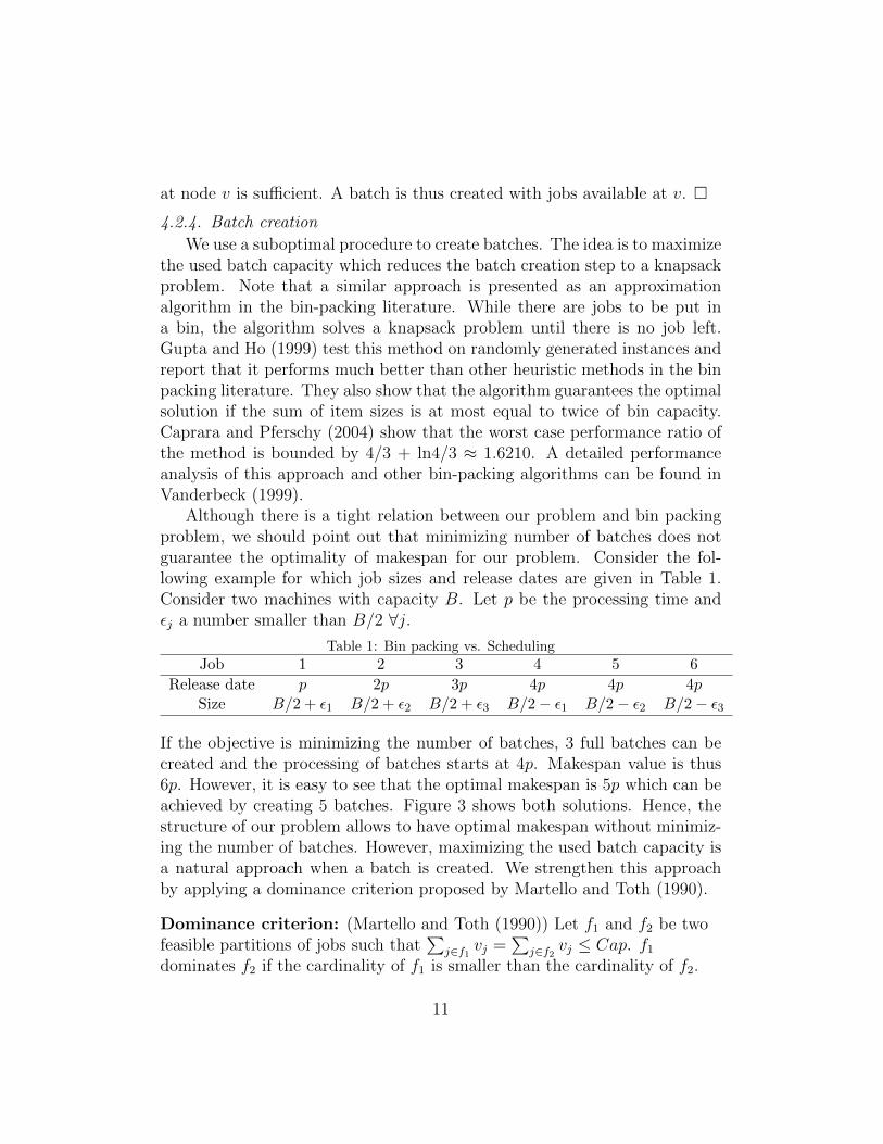
Although there is a tight relation between our problem and bin packingproblem, we should point out that minimizing number of batches does notguarantee the optimality of makespan for our problem. Consider the fol-lowing example for which job sizes and release dates are given in Table 1.Consider two machines with capacity B. Let p be the processing time andεj a number smaller than B/2 ∀j.

Table 1: Bin packing vs. Scheduling

Job 1 2 3 4 5 6

Release date p 2p 3p 4p 4p 4pSize B/2 + ε1 B/2 + ε2 B/2 + ε3 B/2− ε1 B/2− ε2 B/2− ε3

If the objective is minimizing the number of batches, 3 full batches can becreated and the processing of batches starts at 4p. Makespan value is thus6p. However, it is easy to see that the optimal makespan is 5p which can beachieved by creating 5 batches. Figure 3 shows both solutions. Hence, thestructure of our problem allows to have optimal makespan without minimiz-ing the number of batches. However, maximizing the used batch capacity isa natural approach when a batch is created. We strengthen this approachby applying a dominance criterion proposed by Martello and Toth (1990).

Dominance criterion: (Martello and Toth (1990)) Let f1 and f2 be twofeasible partitions of jobs such that

∑j∈f1 vj =

∑j∈f2 vj ≤ Cap. f1

dominates f2 if the cardinality of f1 is smaller than the cardinality of f2.

11

Jobs 1, 4

machines

4p 5p 6p

21

Jobs 2, 5

Jobs 3, 6 Job 1

machines

p 2p 3p 4p 5p

21

Job 2 Job 3 Jobs 4, 5

Job 6

time time

Solution with 3 batches Solution with 5 batches

Figure 3: Two solutions for the example presented in Table 1

The dominance criterion above prioritizes big size jobs for batch creation.This way, if there are other big size jobs released later and if these jobs cannotbe batched with earlier big size jobs, the idea of the dominance criterionis to leave smaller size jobs to later instants. For that purpose, a binarysearch procedure is used to create a single batch. If there are many batchconfigurations, binary search procedure chooses the one containing the leastnumber of jobs. This procedure, named (createBatch(.)), is presented in theappendix.

4.2.5. Initialization: Upper bound heuristic

We use a heuristic to find an upper value on makespan at the root node.This heuristic creates batches with consecutive jobs. If a job cannot be placedin a batch because of capacity limitations, batch is closed and assigned tothe machine having the smallest idle time.

4.2.6. Numerical example

Consider the example given in Figure 1. Figure 4 shows the search treefor the example. Numbers in nodes represent the order of visiting nodesin the search tree. Lower bound values associated with each child node isrepresented next to branches. We explain below the solution procedure stepby step.

Solution steps for the numerical example

Heuristic finds an upper bound value equal to 140. The initial lower boundis 100.Node 1 (root node): Left branch represents delaying the processing of job

12

1

52

LBroot

= 100

UBroot

= 140

3

4

6

7

8x

x x

x

100 130

100

100

160

150

140 130130

130

130

Cmax

* = 130 < 140

x 130

Figure 4: The search tree for the example

1 until the release of second job which provides a lower bound value smallerthan processing job 1 immediately upon its release. Thus, left branching isprioritized.Nodes 2, 3 and 4: Delaying the processing of jobs 1,2 and 3 until therelease of job 4 gives a lower bound value smaller than right branching atnodes 2 and 3. Thus, left child nodes are visited first. At node 4, all jobs areavailable. Right branching at node 4 represents the processing of jobs 1 and2 in the same batch at instant 40. But the lower bound value of the childnode is 160. This branch is thus pruned.Backtracking at Node 3: Left branch at node 3 processes jobs 1 and 2 inthe same batch at instant 30. But with the remaining jobs, at least two otherbatches are created and thus the lower bound associated with that branchbecomes 150. It is thus pruned.Backtracking at Node 2: Left branch at node 2 processes jobs 1 and 2 inthe same batch at instant 20. Since the lower bound associated with the rightchild node is equal to 140, i.e. current best makespan value, right branch ispruned.Backtracking at Node 1 and right branching: Job 1 is processed onmachine 1 at instant 10.Node 5: Left branch has a lower bound value equal to that of right branchat node 5. Job 2, which is available at node 5, is thus delayed.

13

Node 6: Left and right branches has equal lower bound value. Tie is brokenby choosing left branch.Node 7: All unprocessed jobs are available at node 7. Job 1 has alreadybeen processed. Machine 1 is idle at 70 and machine two is idle at 0. Jobs 2and 4 are put is the same batch and processed at instant 40 on machine 2.Node 8: Finally, job 3 is processed on machine 1 which gives a makespanvalue equal to 130 (130 becomes the new best Cmax value).Backtracking at nodes 6 and 5: The lower bound values associated withthe right branches of nodes 6 and 5 are greater or equal to 130. Thesebranches are thus pruned.

Figure 5 shows the Gantt Diagram corresponding to the optimal solution.

Job 1

Job 2, Job 4

machines

10 40 70 100 130 time

21

Job 3

Figure 5: Solution of the numerical example with branch and bound

Pseudo-code of the algorithm is given in appendix.

4.2.7. Optimally solvable cases

Ikura and Gimple (1986) studied a special case of our problem where jobshave unit sizes and presented a polynomial time algorithm. It is straight-forward to see that B&BH guarantees the optimal solution if all jobs havethe same size in a problem instance since batch creation becomes easy. Wenow present another special case that B&BH can guarantee optimal solution.Suppose for any time interval of length of p/m, sum of job sizes is smalleror equal to machine capacity for jobs whose release dates are in that timeinterval. We first show that in this special case makespan value is equal torn + p and then argue that B&BH finds optimal solution.

Property 1. Suppose for any a time interval [rj, rj + p/m] the sum ofjob sizes is smaller or equal to the machine capacity, i.e.

∑wk ≤ B ∀k such

that rk ∈ [rj, rj + p/m] ∀j. Then, the optimum makespan value is equal torn + p where rn is the last job release date.

Proof. Let K be an integer such that r1 ∈ [rn−K∗p/m, rn−(K−1)∗p/m].Then, we have K intervals of length p/m which allows us to create K batches.

14

Considering the first batch is processed at instant rn−(K−1)∗p/m, a secondbatch can be created and processed at rn−(K−2)∗p/m on machine 2. Then,the second batch on machine 1 is created with jobs whose release dates arein [rn − (K −m) ∗ p/m, rn − (K − (m+ 1)) ∗ p/m] and processed at most atinstant rn − (K − (m + 1)) ∗ p/m. Observe that rn − (K − (m + 1)) ∗ p/mis equal to the processing ending time of the first batch on machine 1, i.e.rn − (K − 1) ∗ p/m + p. Similarly, jobs having release dates in the interval[rn − p/m, rn] are processed at rn which concludes the proof. �

In this special case, since B&BH explores instants at which only a singlebatch can be created, batch creation is no longer a difficult task and thusB&BH gives the optimal makespan thanks to exploring every possible instantin the problem.

5. Computational experiments

In this section, we test two types of problem instances which are inspiredfrom the hospital sterilization context. Algorithms are coded in Java andimplemented on an Intel Core i5 2.50 GHz machine. Solution time limit isset to one hour. We use the genetic algorithm of Wang and Chou (2010)noted GALit, approximation algorithm of Li (2012) noted AALit and theMILP model of Ozturk et al. (2012) noted MILPLit for benchmarking.

MILPLit can guarantee the optimal solution once a problem instance iscompletely solved. GALit is a powerful meta-heuristic which provides slightlybetter results in terms of solution quality and solution time compared to othermeta-heuristics from the literature. Briefly, GALit generates chromosomes ateach iteration by randomization and immigration, and then performs a twopoint cross over between chromosomes chosen with the roulette wheel tech-nique. AALit solves the problem initially by allowing jobs to be split. Andthen split jobs are scheduled by being assigned individually to a batch follow-ing the last batch in the lower bound solution. To the best of our knowledge,the performance of approximation algorithms in the batch scheduling liter-ature, including the one proposed by Li (2012), have not been tested onnumerical instances. It would be thus interesting to observe how AALit per-forms on our instances. For all these reasons, we choose these three methodsfor benchmarking.

Before proceeding with the testing of instances inspired from the ster-ilization context, we tested B&BH on many small instances which can besolved quickly by MILPLit. This way, we compared makespan values found

15

by B&BH to optimal solutions given by MILPLit. For that purpose, wegenerated 20000 test instances containing 6 to 10 jobs in the presence of 1to 4 machines (1000 problem instances are generated for each combinationof number of jobs and number of machines). Job sizes are generated froma discrete uniform distribution: U[1, 120]. p = 60 minutes being the jobprocessing time, r1 = 0 being the first job release date in any instance, jobrelease dates are generated using the following formula: rj = rj−1 + U [0, 30]∀j = 2, ..., n. Among 20000 instances, only 34 of them could not be solvedoptimally by B&BH . This observation encouraged us about the solutionquality of B&BH . Thus we proceeded with a detailed analysis of B&BH bytesting real life instances.

5.1. First instance type: Irregular job arrivals

In some hospitals, RMD sets are sent to the sterilization service justafter the end of a surgery. Thus, RMD arrivals can happen at any timewithin a day. An example of this kind of organization can be found atthe sterilization service of the ambulatory surgery department of UniversityHospital Gasthuisberg in Leuven, Belgium.

Supposing there are surgeries at operating blocks during 8 to 10 hoursper day, job release dates are created according to the uniform distributionU[0, 600] (unit in minutes). The size of automatic washers can be between6 and 12 din. (Din is a measurement unit for the volume of automaticwashers which is about 0.003 m3.) Fixing the machine capacity to 12 din,we create job sizes according to a continuous uniform distribution such thatwj = Uc]0, 12] since any RMD set size smaller than machine capacity ispossible. A washing cycle is 60 minutes. Number of machines is varied from1 to 4. For each combination of number of jobs and number of machines, 20problem instances are generated and solved through this section.

5.1.1. Medium size instances

Medium size instances contain 10 to 40 jobs. For all instances tested in Table2, B&BH is able to give the best solution each time except for one. Let usdetail our analysis by providing more insights about the quality of solutionprovided by B&BH and other methods. In Table 2, column #NB (not best)indicates the number of times a method does not provide the best solution.Avg. gap shows the average of gap for instances whose makespan value isnot equal to the best one. The formula used for Avg. gap is the following:(Solutionmethod − best solution) / best solution.

16

Table 2: Benchmarking results on medium size instances for irregular arrivalsB&BH MILPLit GALit AALit

No. No. # Avg. # Avg. # Avg. # Avg.mach. Jobs NB gap NB gap NB gap NB gap

10 - - - - - - 1 14%1 20 - - - - - - 2 10%

30 1 ≈ 0 - - 4 5% 5 12%40 - - 7 5% 5 6% 5 12%10 - - - - - - 1 10%

2 20 - - - - - - 1 4%30 - - - - 4 2% 5 6%40 - - 6 4% 3 4% 3 10%10 - - - - - - - -

3 20 - - - - - - - -30 - - - - - - 1 ≈ 040 - - 7 1% - - 1 ≈ 010 - - - - - - - -

4 20 - - - - - - - -30 - - - - - - 1 ≈ 040 - - 2 1% - - 2 ≈ 0

For instances containing more than 10 jobs, MILP cannot find the opti-mal solution within one hour. Nevertheless, it can provide the best solutionfor all instances containing 10, 20 and 30 jobs (The optimality gap reportedby CPLEX is around 10% for instances with 30 jobs at the end of one hour).Starting from 40 job instances, performance of MILPLit decreases. Regard-ing GALit and AALit, their performances increase with the increasing numberof machines since it becomes easier to find an idle machine for the processingof a batch. In the presence of one and two machines, solution quality ofthese heuristics are not satisfactory. However, their solution times are faster.AALit can find a solution within some milliseconds. The maximum solutiontime with GALit is 10 seconds. A detailed presentation of average solutiontimes for all irregular type instances is given in Table 5.

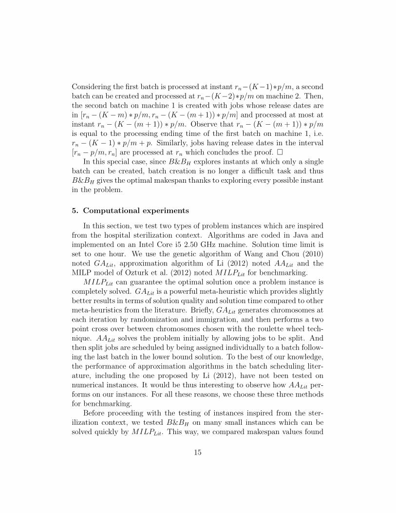
B&BH can quickly find a solution for instances containing up to 40 jobs inthe presence of a single machine. The branching scheme and quality of upperand lower bound algorithms play an important role for the solution time.Table 3 shows the quality of the lower bound algorithm and the initializationheuristic as well as the number of nodes created by B&BH and the averagesolution times in seconds. Columns 4 and 5 show the average and maximumgaps between lower bound andB&BH which is calculated as (SolutionB&BH

−

17

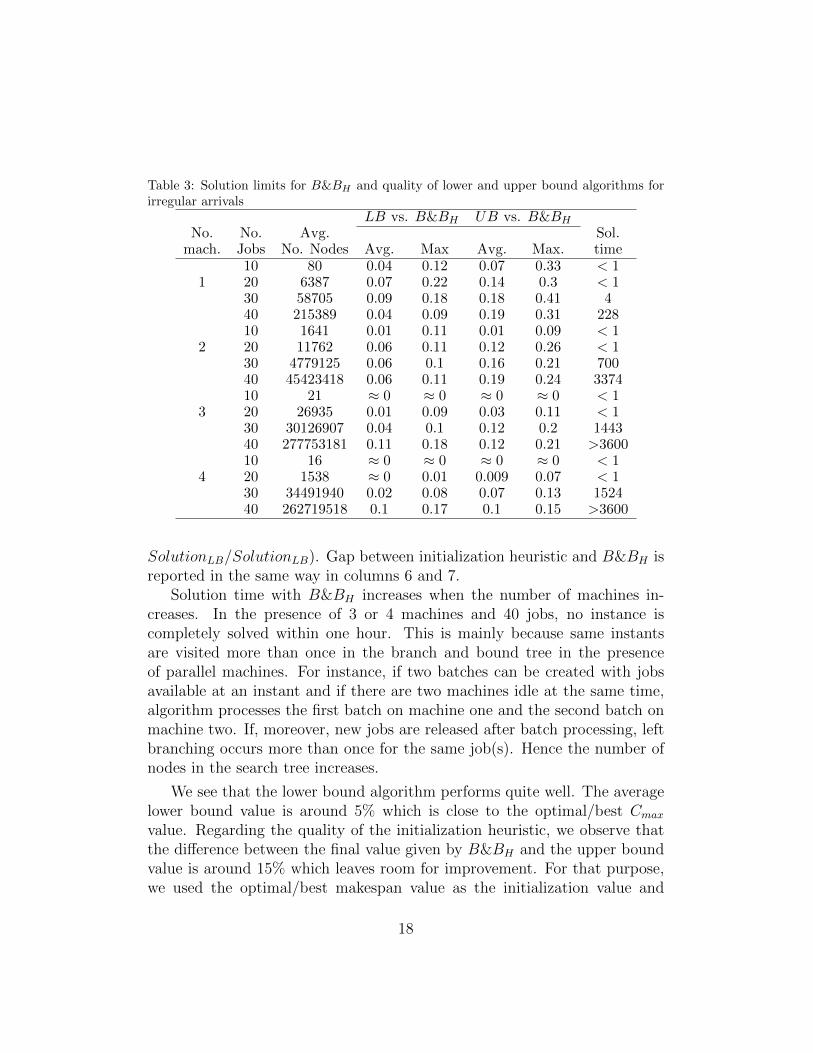
Table 3: Solution limits for B&BH and quality of lower and upper bound algorithms forirregular arrivals

LB vs. B&BH UB vs. B&BH

No. No. Avg. Sol.mach. Jobs No. Nodes Avg. Max Avg. Max. time

10 80 0.04 0.12 0.07 0.33 < 11 20 6387 0.07 0.22 0.14 0.3 < 1

30 58705 0.09 0.18 0.18 0.41 440 215389 0.04 0.09 0.19 0.31 22810 1641 0.01 0.11 0.01 0.09 < 1

2 20 11762 0.06 0.11 0.12 0.26 < 130 4779125 0.06 0.1 0.16 0.21 70040 45423418 0.06 0.11 0.19 0.24 337410 21 ≈ 0 ≈ 0 ≈ 0 ≈ 0 < 1

3 20 26935 0.01 0.09 0.03 0.11 < 130 30126907 0.04 0.1 0.12 0.2 144340 277753181 0.11 0.18 0.12 0.21 >360010 16 ≈ 0 ≈ 0 ≈ 0 ≈ 0 < 1

4 20 1538 ≈ 0 0.01 0.009 0.07 < 130 34491940 0.02 0.08 0.07 0.13 152440 262719518 0.1 0.17 0.1 0.15 >3600

SolutionLB/SolutionLB). Gap between initialization heuristic and B&BH isreported in the same way in columns 6 and 7.

Solution time with B&BH increases when the number of machines in-creases. In the presence of 3 or 4 machines and 40 jobs, no instance iscompletely solved within one hour. This is mainly because same instantsare visited more than once in the branch and bound tree in the presenceof parallel machines. For instance, if two batches can be created with jobsavailable at an instant and if there are two machines idle at the same time,algorithm processes the first batch on machine one and the second batch onmachine two. If, moreover, new jobs are released after batch processing, leftbranching occurs more than once for the same job(s). Hence the number ofnodes in the search tree increases.

We see that the lower bound algorithm performs quite well. The averagelower bound value is around 5% which is close to the optimal/best Cmax

value. Regarding the quality of the initialization heuristic, we observe thatthe difference between the final value given by B&BH and the upper boundvalue is around 15% which leaves room for improvement. For that purpose,we used the optimal/best makespan value as the initialization value and

18

tested some of the same problem instances. We observed that there is almostno improvement in the solution time. Then, for the same instances, weforced the initial makespan value to be equal to a very big number. Weobserved that the average solution time increased by an average of 1%. Wecan thus conclude that the performance of the initialization heuristic is goodfor decreasing the solution time.

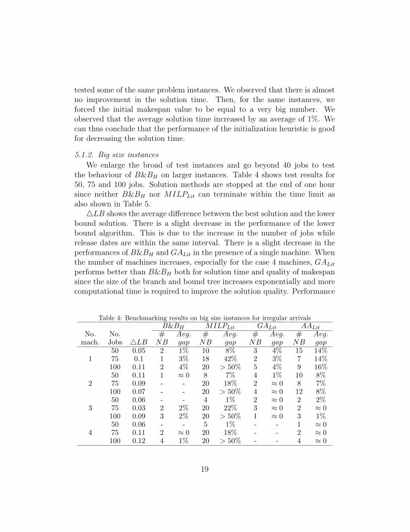
5.1.2. Big size instances

We enlarge the broad of test instances and go beyond 40 jobs to testthe behaviour of B&BH on larger instances. Table 4 shows test results for50, 75 and 100 jobs. Solution methods are stopped at the end of one hoursince neither B&BH nor MILPLit can terminate within the time limit asalso shown in Table 5.4LB shows the average difference between the best solution and the lower

bound solution. There is a slight decrease in the performance of the lowerbound algorithm. This is due to the increase in the number of jobs whilerelease dates are within the same interval. There is a slight decrease in theperformances of B&BH and GALit in the presence of a single machine. Whenthe number of machines increases, especially for the case 4 machines, GALit

performs better than B&BH both for solution time and quality of makespansince the size of the branch and bound tree increases exponentially and morecomputational time is required to improve the solution quality. Performance

Table 4: Benchmarking results on big size instances for irregular arrivalsB&BH MILPLit GALit AALit

No. No. # Avg. # Avg. # Avg. # Avg.mach. Jobs 4LB NB gap NB gap NB gap NB gap

50 0.05 2 1% 10 8% 3 4% 15 14%1 75 0.1 1 3% 18 42% 2 3% 7 14%

100 0.11 2 4% 20 > 50% 5 4% 9 16%50 0.11 1 ≈ 0 8 7% 4 1% 10 8%

2 75 0.09 - - 20 18% 2 ≈ 0 8 7%100 0.07 - - 20 > 50% 4 ≈ 0 12 8%50 0.06 - - 4 1% 2 ≈ 0 2 2%

3 75 0.03 2 2% 20 22% 3 ≈ 0 2 ≈ 0100 0.09 3 2% 20 > 50% 1 ≈ 0 3 1%50 0.06 - - 5 1% - - 1 ≈ 0

4 75 0.11 2 ≈ 0 20 18% - - 2 ≈ 0100 0.12 4 1% 20 > 50% - - 4 ≈ 0

19

Table 5: Summary of average solution times in seconds for irregular arrivalsNumber of jobs

Method No.mach 10 20 30 40 50 75 100MILPLit <1 >3600 >3600 >3600 >3600 >3600 >3600BBH 1 <1 <1 4 228 >3600 >3600 >3600GALit <1 2 4 8 18 25 62AALit <1 <1 <1 <1 <1 <1 <1

MILPLit <1 >3600 >3600 >3600 >3600 >3600 >3600BBH 2 <1 <1 700 3374 >3600 >3600 >3600GALit <1 <1 8 9 28 24 61AALit <1 <1 <1 <1 <1 <1 <1

MILPLit <1 >3600 >3600 >3600 >3600 >3600 >3600BBH 3 <1 <1 1443 >3600 >3600 >3600 >3600GALit <1 <1 5 4 35 31 40AALit <1 <1 <1 <1 <1 <1 <1

MILPLit <1 >3600 >3600 >3600 >3600 >3600 >3600BBH 4 <1 <1 1524 >3600 >3600 >3600 >3600GALit <1 <1 6 5 32 42 50AALit <1 <1 <1 <1 <1 <1 <1

of AALit also decreases in these big instances due to the increasing differencebetween the lower bound and optimal makespan values.

5.2. Second instance type: Regular arrivals

These test instances are inspired from the sterilization service of GrenobleUniversity Hospital. RMD sets are sent to the sterilization service twice aday: early in the morning and in the afternoon. RMD sets arriving in themorning are those used the day before. Ones sent in the afternoon are thoseused in surgeries in the morning. Regarding these informations, we imposetwo different release dates for job arrivals: 0 and rmax/2 where rmax standsfor the closing time of the service. Considering the sterilization service isopen 10 hours per day, rmax = 600. We assume that half of the jobs arereleased at instant 0 and half of them at rmax/2.

Tables 6 and 7 summarize the test results for quality of makespan andsolution time, respectively. There is a considerable decrease in the solutiontime of B&BH due to having only two different release dates. Left branchingis done a few times and thus number of nodes also decreases. Regarding thequality of the lower bound algorithm, we observe that it gives similar resultscompared to those in irregular arrivals in the presence of medium size jobs.

20

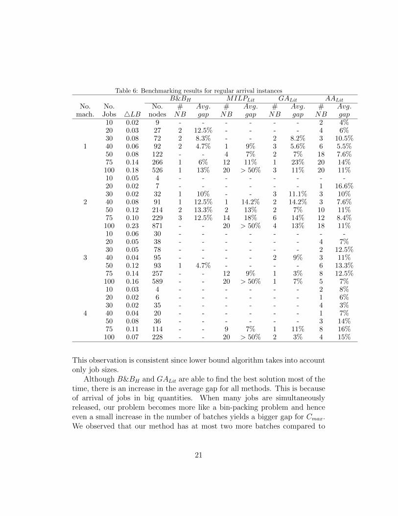
Table 6: Benchmarking results for regular arrival instancesB&BH MILPLit GALit AALit

No. No. No. # Avg. # Avg. # Avg. # Avg.mach. Jobs 4LB nodes NB gap NB gap NB gap NB gap

10 0.02 9 - - - - - - 2 4%20 0.03 27 2 12.5% - - - - 4 6%30 0.08 72 2 8.3% - - 2 8.2% 3 10.5%

1 40 0.06 92 2 4.7% 1 9% 3 5.6% 6 5.5%50 0.08 122 - - 4 7% 2 7% 18 7.6%75 0.14 266 1 6% 12 11% 1 23% 20 14%100 0.18 526 1 13% 20 > 50% 3 11% 20 11%10 0.05 4 - - - - - - - -20 0.02 7 - - - - - - 1 16.6%30 0.02 32 1 10% - - 3 11.1% 3 10%

2 40 0.08 91 1 12.5% 1 14.2% 2 14.2% 3 7.6%50 0.12 214 2 13.3% 2 13% 2 7% 10 11%75 0.10 229 3 12.5% 14 18% 6 14% 12 8.4%100 0.23 871 - - 20 > 50% 4 13% 18 11%10 0.06 30 - - - - - - - -20 0.05 38 - - - - - - 4 7%30 0.05 78 - - - - - - 2 12.5%

3 40 0.04 95 - - - - 2 9% 3 11%50 0.12 93 1 4.7% - - - - 6 13.3%75 0.14 257 - - 12 9% 1 3% 8 12.5%100 0.16 589 - - 20 > 50% 1 7% 5 7%10 0.03 4 - - - - - - 2 8%20 0.02 6 - - - - - - 1 6%30 0.02 35 - - - - - - 4 3%

4 40 0.04 20 - - - - - - 1 7%50 0.08 36 - - - - - - 3 14%75 0.11 114 - - 9 7% 1 11% 8 16%100 0.07 228 - - 20 > 50% 2 3% 4 15%

This observation is consistent since lower bound algorithm takes into accountonly job sizes.

Although B&BH and GALit are able to find the best solution most of thetime, there is an increase in the average gap for all methods. This is becauseof arrival of jobs in big quantities. When many jobs are simultaneouslyreleased, our problem becomes more like a bin-packing problem and henceeven a small increase in the number of batches yields a bigger gap for Cmax.We observed that our method has at most two more batches compared to

21

Table 7: Summary of average solution times in seconds for regular arrivalsNumber of jobs

Method No.mach 10 20 30 40 50 75 100MILPLit <1 >3600 >3600 >3600 >3600 >3600 >3600BBH 1 <1 <1 <1 <1 <1 62 1084GALit <1 <1 2 3 18 22 61AALit <1 <1 <1 <1 <1 <1 <1

MILPLit <1 604 >3600 >3600 >3600 >3600 >3600BBH 2 <1 <1 <1 <1 <1 61 1300GALit <1 <1 1 2 12 29 32AALit <1 <1 <1 <1 <1 <1 <1

MILPLit <1 422 >3600 >3600 >3600 >3600 >3600BBH 3 <1 <1 <1 <1 <1 73 1502GALit <1 <1 1 3 9 31 45AALit <1 <1 <1 <1 <1 <1 <1

MILPLit <1 309 >3600 >3600 >3600 >3600 >3600BBH 4 <1 <1 <1 <1 <1 80 1480GALit <1 <1 <1 5 15 25 37AALit <1 <1 <1 <1 <1 <1 <1

the number of batches in the solution giving the best makespan value unlessprovided by B&BH . This observation is in line with the bin packing resultsgiven in Vanderbeck (1999). Regarding MILPLit, it gives the best solutionfor instances containing less or equal to 30 jobs. However, it requires toomuch computation. While B&BH finds a solution within some seconds, theoptimality gap is more than 50% with MILPLit at the end of 300 secondsfor the case of a single machine.

As in the case of irregular arrivals, the performance of the lower boundalgorithm decreases when the number of jobs increases. However, this situa-tion has almost no impact on the solution time with B&BH since the size ofthe search tree is small due to having two different job release dates. WhileMILPLit is not able to provide a better makespan value for instances con-taining more than 40 or 50 jobs depending on the number of machines, ourmethod is able to compete with GALit in the presence of a few machines.When the number of machines increases, B&BH performs better than othermethods. Regarding solution times of other methods, AALit is very fast andit can find a solution within some miliseconds. GALit on the other hand hasan increase in its solution time. It can provide a solution in less than oneminute for big size instances.

22

6. Conclusions

In this paper, we studied a parallel batch scheduling problem whose originis hospital sterilization services. Jobs have different sizes, different releasedates and equal processing times. Our objective is to minimize the makespanon parallel identical machines. MILP models in the literature require longcomputation time for real size instances. Heuristic methods are faster butdo not guarantee the optimality for makespan. We presented a branch andbound based heuristic method which can solve instances containing up to 40jobs within very short time. We tested this method on real life instancesand compared the solution quality to other methods from the literature.Numerical results show that our method can provide high quality makespanvalues in reasonable computational time.

Many extensions of our problem can be considered for future work. Con-sidering there is imperfect knowledge about job arrivals at the steriliza-tion service, uncertain job release dates may be considered. Some dynamicstochastic approaches (e.g., rolling horizon method) can be applied to thisnew case instead of deterministic methods. Moreover, some other objectivefunctions (e.g.,

∑Cj) can be studied.

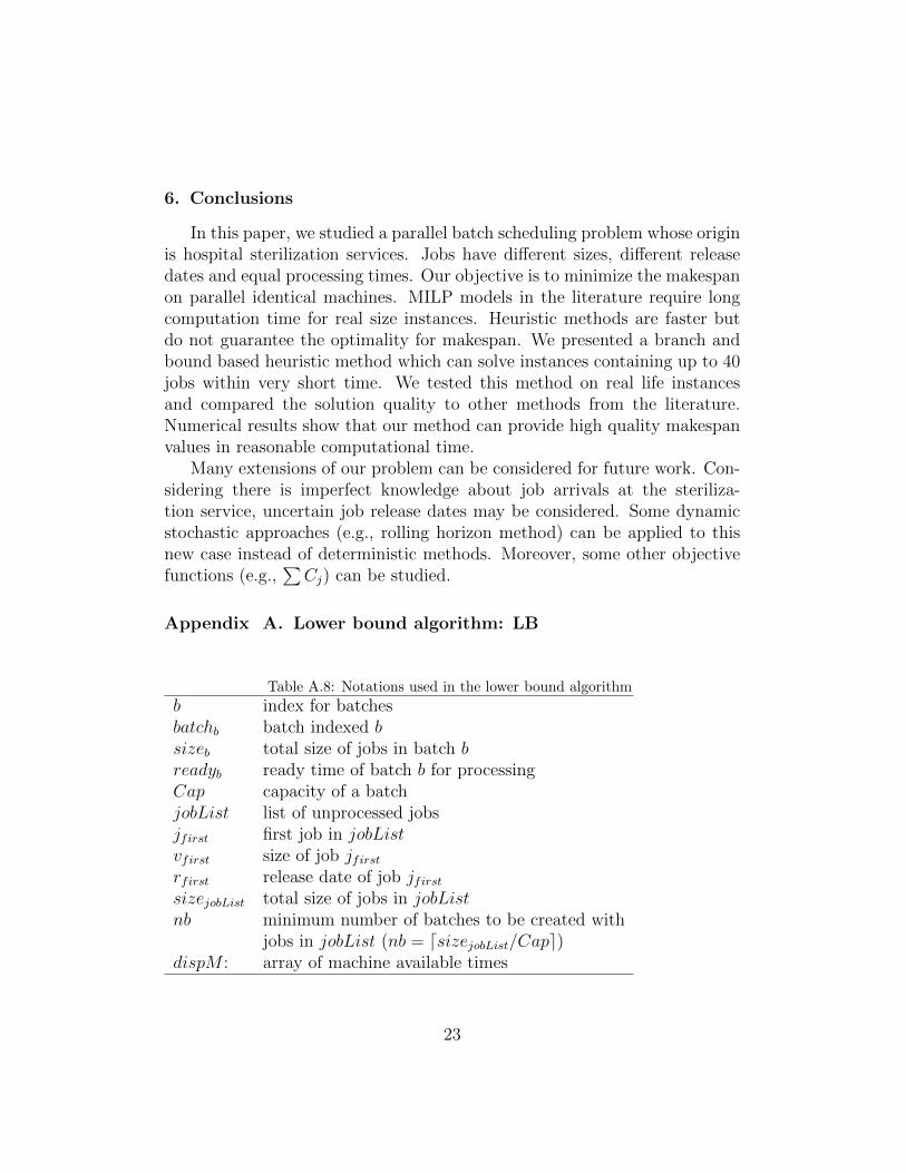
Appendix A. Lower bound algorithm: LB

Table A.8: Notations used in the lower bound algorithm

b index for batchesbatchb batch indexed bsizeb total size of jobs in batch breadyb ready time of batch b for processingCap capacity of a batchjobList list of unprocessed jobsjfirst first job in jobListvfirst size of job jfirstrfirst release date of job jfirstsizejobList total size of jobs in jobListnb minimum number of batches to be created with

jobs in jobList (nb = dsizejobList/Cape)dispM : array of machine available times

23

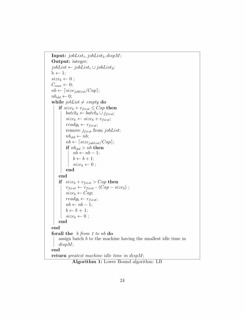
Input: jobList1, jobList2, dispM ;Output: integer;jobList← jobList1 ∪ jobList2;b ← 1;sizeb ← 0 ;Cmax ← 0;nb← dsizejobList/Cape;nbold ← 0;while jobList 6= empty do

if sizeb + vfirst ≤ Cap thenbatchb ← batchb ∪ jfirst;sizeb ← sizeb + vfirst;readyb ← rfirst;remove jfirst from jobList;nbold ← nb;nb← dsizejobList/Cape;if nbold > nb then

nb← nb− 1;b← b+ 1;sizeb ← 0 ;

end

endif sizeb + vfirst > Cap then

vfirst ← vfirst - (Cap− sizeb) ;sizeb ← Cap;readyb ← rfirst;nb← nb− 1;b← b + 1;sizeb ← 0 ;

end

endforall the b from 1 to nb do

assign batch b to the machine having the smallest idle time indispM ;

endreturn greatest machine idle time in dispM ;

Algorithm 1: Lower Bound algorithm: LB

24

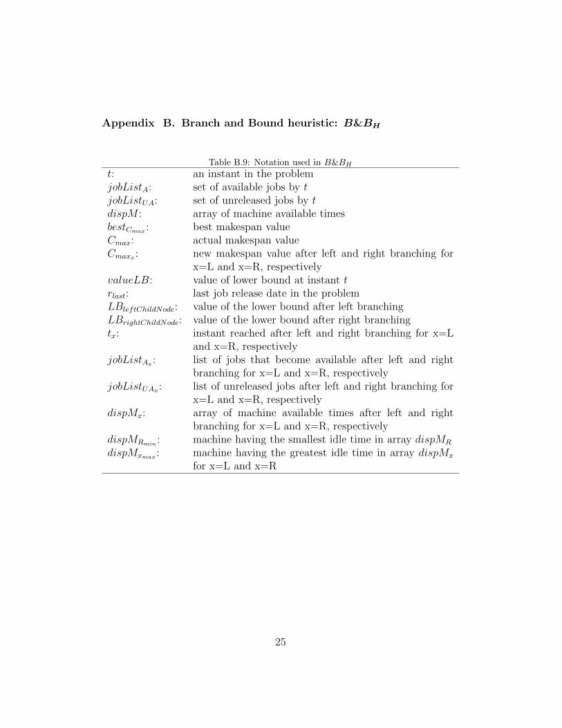
Appendix B. Branch and Bound heuristic: B&BH

Table B.9: Notation used in B&BH

t: an instant in the problemjobListA: set of available jobs by tjobListUA: set of unreleased jobs by tdispM : array of machine available timesbestCmax : best makespan valueCmax: actual makespan valueCmaxx : new makespan value after left and right branching for

x=L and x=R, respectivelyvalueLB: value of lower bound at instant trlast: last job release date in the problemLBleftChildNode: value of the lower bound after left branchingLBrightChildNode: value of the lower bound after right branchingtx: instant reached after left and right branching for x=L

and x=R, respectivelyjobListAx : list of jobs that become available after left and right

branching for x=L and x=R, respectivelyjobListUAx : list of unreleased jobs after left and right branching for

x=L and x=R, respectivelydispMx: array of machine available times after left and right

branching for x=L and x=R, respectivelydispMRmin

: machine having the smallest idle time in array dispMR

dispMxmax : machine having the greatest idle time in array dispMx

for x=L and x=R

25

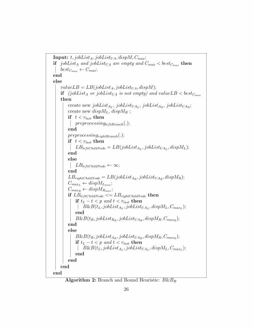
Input: t, jobListA, jobListUA, dispM,Cmax;if jobListA and jobListUA are empty and Cmax < bestCmax then

bestCmax ← Cmax;endelse

valueLB = LB(jobListA, jobListUA, dispM);if (jobListA or jobListUA is not empty) and valueLB < bestCmax

thencreate new jobListAL

, jobListUAL, jobListAR

, jobListUAR;

create new dispML, dispMR ;if t < rlast then

preprocessingleftBranch(.);endpreprocessingrightBranch(.);if t < rlast then

LBleftChildNode = LB(jobListAL, jobListUAL

, dispML);endelse

LBleftChildNode ←∞;endLBrightChildNode = LB(jobListAR

, jobListUAR, dispMR);

CmaxL← dispMLmax ;

CmaxR← dispMRmax ;

if LBleftChildNode <= LBrightChildNode thenif tL − t < p and t < rlast then

B&B(tL, jobListAL, jobListUAL

, dispML, CmaxL);

endB&B(tR, jobListRR

, jobListUAR, dispMR, CmaxR

);endelse

B&B(tR, jobListAR, jobListUAR

, dispMR, CmaxR);

if tL − t < p and t < rlast thenB&B(tL, jobListAL

, jobListUAL, dispML, CmaxL

);end

end

end

end

Algorithm 2: Branch and Bound Heuristic: B&BH

26

Input: tL, jobListA, jobListUA, dispM, jobListAL, jobListUAL

, dispML

;tL ← release date of first job in jobListUA;jobListAL

← jobListA∪ job(s) j in jobListUA such that rj <= tL;jobListUAL

← jobListUA− job(s) j in jobListUA such that rj <= tL;dispML ← dispM ;

Algorithm 3: preprocessingleftBranch()

Input:t, tR, jobListA, jobListUA, dispM, jobListAR

, jobListUAR, dispMR;

jobListAR← jobListA;

jobListUAR← jobListUA;

create new jobsInBatch;jobsInBatch← createBatch(jobListAR

, 0, jobsInBatch, 0);jobListAR

← jobListAR− jobsInBatch;

dispMR ← dispM ;dispMRmin

← max(t, dispMRmin) + p;

if jobListARis not empty then

tR ← dispMRmin;

endelse

tR ← max(dispMRmin, first job release date in jobListUAR

) ;endjobListAR

← jobListAR∪ job(s) j in jobListUR such that rj <= tR;

jobListUAR← jobListUR− job(s) j in jobListUR such that rj <= tR;

Algorithm 4: preprocessingrightBranch()

Table B.10: Notations used in batch creation procedure

jobList: list of available jobs for batchingindex: an integer representing job indexesusedCapacity: used capacity of the batchjobsInBatch: jobs in batchbestV alue: value of the best capacity utilization in the current best solutionjobListk: kth job in jobListsolutionGlobal: jobs put in batch in the current best solution

27

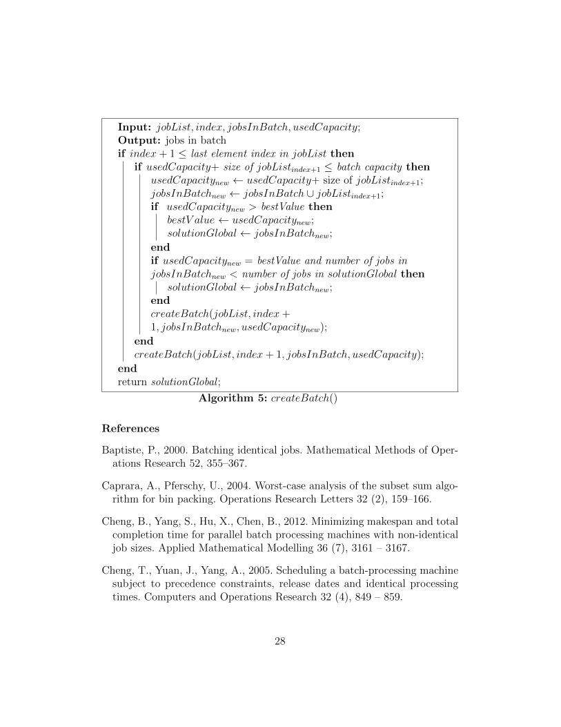
Input: jobList, index, jobsInBatch, usedCapacity;Output: jobs in batchif index+ 1 ≤ last element index in jobList then

if usedCapacity+ size of jobListindex+1 ≤ batch capacity thenusedCapacitynew ← usedCapacity+ size of jobListindex+1;jobsInBatchnew ← jobsInBatch ∪ jobListindex+1;if usedCapacitynew > bestValue then

bestV alue ← usedCapacitynew;solutionGlobal← jobsInBatchnew;

endif usedCapacitynew = bestValue and number of jobs injobsInBatchnew < number of jobs in solutionGlobal then

solutionGlobal← jobsInBatchnew;endcreateBatch(jobList, index+1, jobsInBatchnew, usedCapacitynew);

endcreateBatch(jobList, index+ 1, jobsInBatch, usedCapacity);

endreturn solutionGlobal ;

Algorithm 5: createBatch()

References

Baptiste, P., 2000. Batching identical jobs. Mathematical Methods of Oper-ations Research 52, 355–367.

Caprara, A., Pferschy, U., 2004. Worst-case analysis of the subset sum algo-rithm for bin packing. Operations Research Letters 32 (2), 159–166.

Cheng, B., Yang, S., Hu, X., Chen, B., 2012. Minimizing makespan and totalcompletion time for parallel batch processing machines with non-identicaljob sizes. Applied Mathematical Modelling 36 (7), 3161 – 3167.

Cheng, T., Yuan, J., Yang, A., 2005. Scheduling a batch-processing machinesubject to precedence constraints, release dates and identical processingtimes. Computers and Operations Research 32 (4), 849 – 859.

28

Chou, F., 2007. A joint ga+dp approach for single burn-in oven schedulingproblems with makespan criterion. Int J Adv Manuf Technol 35, 587–595.

Chung, S., Tai, Y., Pearn, W., 2009. Minimizing makespan on parallel batchprocessing machines with non-identical ready time and arbitrary job sizes.International Journal of Production Research 47 (18), 5109–5128.

Damodaran, P., Velez Gallego, M., 2010. Heuristics for makespan minimiza-tion on parallel batch processing machineswith unequal job ready times.International Journal of Advanced Manufacturing Technology 49 (9–12),1119–1128.

Damodaran, P., Velez-Gallego, M., Maya, J., 2011. A grasp approach formakespan minimization on parallel batch processing machines. Journal ofIntelligent Manufacturing 22 (5), 767–777.

Damodaran, P., Velez-Gallego, M. C., 2012. A simulated annealing algorithmto minimize makespan of parallel batch processing machines with unequaljob ready times. Expert Systems with Applications 39 (1), 1451 – 1458.

Di Mascolo, M., Gouin, A., 2013. A generic simulation model to assess theperformance of sterilization services in health establishments. Health caremanagement science 16 (1), 45–61.

Dupont, L., Dhaenens-Flipo, C., 2002. Minimizing the makespan on a batchprocessing machine with non-identical job sizes: an exact procedure. Com-puters and Operations Research 29 (7), 807–819.

Graham, R., Lawler, E., Lenstra, J., Rinnooy Kan, A., 1979. Optimizationand approximation in deterministic sequencing and scheduling: a survey.Annals of Discrete Mathematics 5, 287–326.

Gupta, J. N., Ho, J. C., 1999. A new heuristic algorithm for the one-dimensional bin-packing problem. Production planning & control 10 (6),598–603.

Ikura, Y., Gimple, M., 1986. Efficient scheduling algorithms for a single batchprocessing machine. Operations Research Letters 5 (2), 61–65.

Li, S., 2012. Makespan minimization on parallel batch processing machineswith release times and job sizes. Journal of Software 7 (6), 1203–1210.

29

Li, S., Li, G., Wang, X., Liu, Q., 2005. Minimizing makespan on a singlebatching machine with release times and non-identical job sizes. OperationsResearch Letters 33 (2), 157–164.

Liu, L., Ng, C., Cheng, T., 2014. Scheduling jobs with release dates on par-allel batch processing machines to minimize the makespan. OptimizationLetters 8 (1), 307–318.

Lu, S., Feng, H., Li, X., 2010. Minimizing the makespan on a single parallelbatching machine. Theoretical Computer Science 411 (7–9), 1140–1145.

Malapert, A., Gueret, C., Rousseau, L.-M., 2012. A constraint programmingapproach for a batch processing problem with non-identical job sizes. Eu-ropean Journal of Operational Research 221 (3), 533 – 545.

Martello, S., Toth, P., 1990. Knapsack Problems: Algorithms and ComputerImplementation. John Wiley and Sons.

Mathirajan, M., Sivakumar, A., 2006. A literature review, classification andsimple meta-analysis on scheduling of batch processors in semiconductor.International Journal of Advance Manufacturing Technology 29, 990–1001.

Ozturk, O., Espinouse, M.-L., Di Mascolo, M., Gouin, A., 2012. Makespanminimisation on parallel batch processing machines with non-identicaljob sizes and release dates. International Journal of Production Research50 (20).

Parsa, N., Karimi, B., Kashan, A., 2010. A branch and price algorithmto minimize makespan on a single batch processing machine with non-identical job sizes. Computers and Operations Research 37 (10), 1720–1730.

Pearn, W., Hong, J., Tai, Y., 2013. The burn-in test scheduling problemwith batch dependent processing time and sequence dependent setup time.International Journal of Production Research 51 (6), 1694–1706.

Potts, C., Kovalyov, M., 2000. Scheduling with batching : A review. Euro-pean Journal of Operational Research 120, 228–249.

Uzsoy, R., 1994. Scheduling a single batch processing machine with non-identical job sizes. International Journal of Production Research 32 (7),1615–1635.

30

Vanderbeck, F., 1999. Computational study of a column generation algorithmfor bin packing and cutting stock problems. Mathematical Programming86 (3), 565–594.

Wang, H., Chou, F., 2010. Solving the parallel batch-processing machineswith diferent release times job sizes, and capacity limits by metaheuristics.Expert Systems with Applications: An International Journal 37 (2), 1510–1521.

Yuan, J., Liu, Z., Ng, C., Cheng, T., 2004. The unbounded single machineparallel batch scheduling problem with family jobs and release dates tominimize makespan. Theoretical Computer Science 320 (23), 199 – 212.

Zhang, G., Cai, X., Lee, C., Wong, C., 2001. Minimizing makespan on asingle batch processing machine with nonidentical job sizes. Naval ResearchLogistics 48 (3), 226–240.

31