A New Efficient Algorithm for Fitting Rectangular

8/6/2019 A New Efficient Algorithm for Fitting Rectangular

http://slidepdf.com/reader/full/a-new-efficient-algorithm-for-fitting-rectangular 1/4

A New Efficient Algorithm for Fitting RectangularBoxes and Cubes in 3D

Frank Ditrich, Herbert Suesse and Klaus Voss

Friedrich-Schiller-University Jena, Department of Computer Science

Ernst-Abbe-Platz 2

D-07737 Jena, Germany

Abstract- In this paper, we introduce a new approach for fitting

rectangular boxes and cubes given as a set of voxels in a three-

dimensional voxel space. This extends our work on fitting rectan-

gles and squares described in [6] to three dimensions. It is also

based on our normalization method published in [4] and [5]. Here

we also encounter the problem of normalizing the rotation as it is

necessary for rectangles and squares, but here we have two degen-

erate cases to handle. The first one are cubes, the second one are

rectangular boxes with two edges of equal length and the length

of the third edge different from them. Our method delivers good

fitting results, even if the boxes are heavily distorted for example

by cutting-off vertices.

I. INTRODUCTION

In [6] we introduced a new fitting procedure for rectangles and

squares. In contrast to other authors the objects to be fitted are

described as a point set inside a closed region (whereas often

objects are represented by points lying on their contour). Fur-

thermore, it uses the method of simultanouosly normalizing the

transformation and the shape of the object using area moments

as features, as it can be found in [4] and [5]. We used moments

up to fourth order for the optimization of the shape and to handle

the degenerate case where the rectangle becomes a square. In

this case, the second order moments are not sufficient to prop-

erly normalize the rotation. Advantages of this method are thereduced numerical effort for the optimization process and the

invariance with respect to the transformation group.

Since there are many techniques (e. g. computer tomogra-

phy) which deliver three-dimensional data as output it is also

of interest to develop fitting procedures for three-dimensional

objects.

In this paper we present a procedure for fitting rectangular

boxes (and handling the corresponding degenerate cases) which

are described by a set of voxels in a voxel space representing

the object as a solid and not only forming its boundary.

This research was supported by DAKO GmbH, Jena.

I I. FITTING USING NORMALIZATION

At first we give a short summary of the general principle of ourfitting method.

We have a class T of transformations where each t ∈ T is

described by n parameters ξ1, . . . , ξn. We have also a class of

primitives P (θ), these are the theoretical shapes used for fitting

(e.g. rectangles, circles, cubes etc.). Each primitive is described

by m parameters θ1, . . . , θm. If we are given an object O, we

derive a tuple of features f (O) = (f 1, f 2, f 3, . . . ). At this point

some fitting methods try to solve the problem

||f (O) − f (P (θ))||2 −→ min (1)

by searching the m-dimensional space Θ of all primitives.

In our approach, we choose an appropriate canonical frame

for the class of primitives we fit (e.g. a unit square for the

class of all squares with respect to the similarity transforma-

tion group) and normalize the object to that frame. Suppose

we also normalize the optimal primitive P (θ∗) with the same

transformation, we have to solve the optimization problem

||f (O) − f (P (θ∗))||2 −→ min (2)

It has the effective dimension m − n. Examples with effective

dimension 0 can be found in [4], whereas in [5] examples with

dimension 1 are given.

At the end we get the optimal fitting primitive P (θ∗) by ap-

plying the inverse of the normalization transformation to the so-

lution of the optimization process.

III . FITTING RECTANGULAR BOXES

In this paper we use as transformations the group of similarity

transformations. A similarity transformation in three dimen-

sions can be described by seven parameters (three for the trans-

lational part, three for the rotational part and one for the isotrope

scaling). Rectangular boxes can be described by nine parame-

ters (six for the motion and three for the side lengths). As a

canonical frame we choose a centered, axis-parallel rectangular

box with volume 1, which can be described by two parameters

for two of its side lengths. So here we have an example wherethe optimization problem has effective dimension 2.

0-7803-9134-9/05/$20.00 ©2005 IEEE



As features we use here the volume moments

m pqr =

object

x pyqzrdxdydz

up to fourth order ( p + q + r = 4).

The normalization process is done in the following steps:

A. Translation

As a first step, we normalize the translation T and get

(tx, ty, tz) =

−

m100

m000

,−m010

m000

,−m001

m000

.

From now on we use the central moments m

pqr = µ pqr and we

have m100 = m

010 = m001 = 0.

B. Rotation

For the normalization of the rotation we rotate the object so

that the axes of its inertial ellipsoid coincide with the coordi-

nate axes. The inertial ellipsoid axes are the eigenvectors of the

inertial matrix

I =

m

200 m

110 m

101

m

110 m

020 m

011

m

101 m

011 m

002

.

It is real and symmectric and has three real eigenvalues and

three eigenvectors which are pairwise perpendicular. Here an

ambiguity is introduced, since u and −u are both eigenvectors

there are eight possible rotations. In [2] an heuristic method is

given to select one of this eight tiltings. This is of evidence if

for example the normalized objects shall be compared through

some features, but since we deal only with rectangular boxes

this is uncritical for us. So we choose simply one of the eight

possibilities.

If we describe the rotation by

R = R11 R12 R13

R21 R22 R23

R31 R32 R33

(here det(R) = 1 holds), using

(x + y + z)n =

0≤a,b,c≤na+b+c=n

(a + b + c)!

a! b! c!xaybzc

=

0≤a,b,c≤na+b+c=n

a + b + c

b + c

b + c

c

xaybzc

(see [3]) the moments have to be transformed in the followingway:

m

pqr =

0≤a,b,c≤pa+b+c=p 0≤d,e,f≤q

d+e+f=q 0≤h,i,k≤rh+i+k=r

a + b + c

b + c

· . . .

b + c

c

d + e + f

e + f

e + f

f

h + i + k

i + k

· . . .

i + k

k

· Ra

11Rb12Rc

13Rd21Re

22Rf 23Rh

31Ri32Rk

33 · . . .

m

a+d+h,b+e+i,c+f +k.

After that, we have m

110 = m

101 = m

011 = 0.

C. Scaling

Now we normalize the size by an isotrope scaling S so that

m

000 = 1. The scaling factor α is

α = 3

1

m

000

.

The moments are transformed by the relationship

m

pqr = α p+q+r+3m

pqr .

D. Canonical frame parameters

To determine the two remaining parameters, we use some

higher order moments which have nontrivial values. Suppose

we have a centered axis-parallel rectangular box with side lengthsa, b and c and volume 1 (abc = 1). Then the following moments

can be expressed in terms of a and b (all moments of third order

vanish):

µq200=

a2

12µq400=

a4

80µq220 =

a2b2

144

µq020=

b2

12µq040=

b4

80µq202 =

1

144b2

µq002=

1

12a2b2µq004=

1

80a4b4µq022 =

1

144a2

To determine a and b we have to solve the following opti-

mization problem:

f (a, b) = (m

200 − µq200)2 + (m

020 − µq020)2+

(m

002 − µq002)2 + (m

400 − µq400)2+

(m

040 − µq040)2 + (m

004 − µq004)2+

(m

220 − µq220)2 + (m

202 − µq202)2+

(m

022 − µq022)2

−→ min

subject to 0 < a, b < ∞.



If we have a solution we can easily calculate the corners of

the fitted canonical frame and apply the inverse transform (S ·R ·T )−1 = T −1 ·R−1 ·S −1 to get the optimal fitted rectangular

box for our object.

But as for rectangles, there are also cases were the abovegiven normalization of the rotation fails. The inertial ellipsoid

can degenerate to a sphere or to an ellipsoid with two axes of

equal length. In both cases additional procedures are necessary,

which are described in the following.

IV. HANDLING SPECIAL CASES

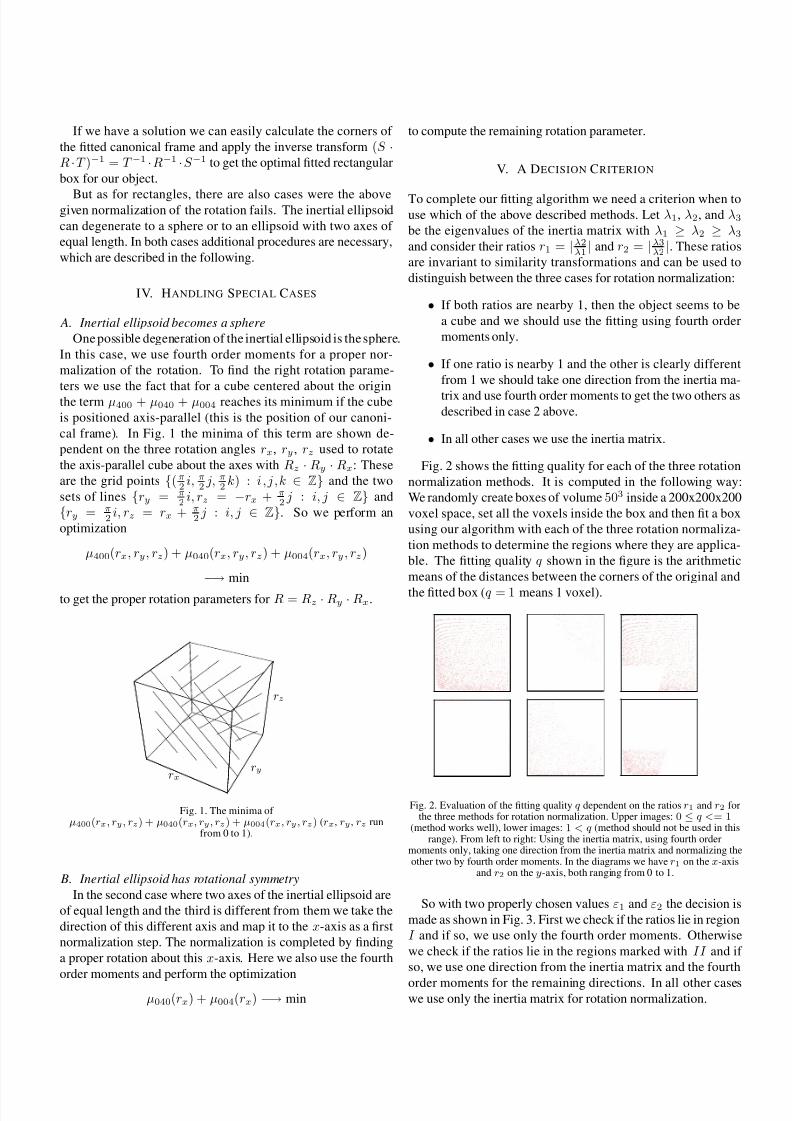
A. Inertial ellipsoid becomes a sphere

One possible degeneration of the inertial ellipsoid is the sphere.

In this case, we use fourth order moments for a proper nor-

malization of the rotation. To find the right rotation parame-

ters we use the fact that for a cube centered about the originthe term µ400 + µ040 + µ004 reaches its minimum if the cube

is positioned axis-parallel (this is the position of our canoni-

cal frame). In Fig. 1 the minima of this term are shown de-

pendent on the three rotation angles rx, ry , rz used to rotate

the axis-parallel cube about the axes with Rz · Ry · Rx: These

are the grid points {(π2

i, π2

j, π2

k) : i,j,k ∈ Z} and the two

sets of lines {ry = π2

i, rz = −rx + π2

j : i, j ∈ Z} and

{ry = π2

i, rz = rx + π2

j : i, j ∈ Z}. So we perform an

optimization

µ400(rx, ry, rz) + µ040(rx, ry, rz) + µ004(rx, ry , rz)

−→ min

to get the proper rotation parameters for R = Rz · Ry · Rx.

rxry

rz

Fig. 1. The minima of µ400(rx, ry, rz) + µ040(rx, ry, rz) + µ004(rx, ry , rz) (rx, ry , rz run

from 0 to 1).

B. Inertial ellipsoid has rotational symmetry

In the second case where two axes of the inertial ellipsoid are

of equal length and the third is different from them we take the

direction of this different axis and map it to the x-axis as a first

normalization step. The normalization is completed by finding

a proper rotation about this x-axis. Here we also use the fourth

order moments and perform the optimization

µ040(rx) + µ004(rx) −→ min

to compute the remaining rotation parameter.

V. A DECISION CRITERION

To complete our fitting algorithm we need a criterion when touse which of the above described methods. Let λ1, λ2, and λ3be the eigenvalues of the inertia matrix with λ1 ≥ λ2 ≥ λ3and consider their ratios r1 = |λ2

λ1| and r2 = |λ3

λ2|. These ratios

are invariant to similarity transformations and can be used to

distinguish between the three cases for rotation normalization:

• If both ratios are nearby 1, then the object seems to be

a cube and we should use the fitting using fourth order

moments only.

• If one ratio is nearby 1 and the other is clearly different

from 1 we should take one direction from the inertia ma-

trix and use fourth order moments to get the two others asdescribed in case 2 above.

• In all other cases we use the inertia matrix.

Fig. 2 shows the fitting quality for each of the three rotation

normalization methods. It is computed in the following way:

We randomly create boxes of volume 503 inside a 200x200x200

voxel space, set all the voxels inside the box and then fit a box

using our algorithm with each of the three rotation normaliza-

tion methods to determine the regions where they are applica-

ble. The fitting quality q shown in the figure is the arithmetic

means of the distances between the corners of the original and

the fitted box (q = 1 means 1 voxel).

Fig. 2. Evaluation of the fitting quality q dependent on the ratios r1 and r2 forthe three methods for rotation normalization. Upper images: 0 ≤ q <= 1

(method works well), lower images: 1 < q (method should not be used in thisrange). From left to right: Using the inertia matrix, using fourth order

moments only, taking one direction from the inertia matrix and normalizing theother two by fourth order moments. In the diagrams we have r1 on the x-axis

and r2 on the y-axis, both ranging from 0 to 1.

So with two properly chosen values ε1 and ε2 the decision is

made as shown in Fig. 3. First we check if the ratios lie in region

I and if so, we use only the fourth order moments. Otherwise

we check if the ratios lie in the regions marked with II and if

so, we use one direction from the inertia matrix and the fourth

order moments for the remaining directions. In all other caseswe use only the inertia matrix for rotation normalization.



ε1

ε1

ε2

ε2

0 1

1

I

II

II

II I

Fig. 3. The regions for the three rotation normalization methods.

r1r2

4

0

0

10

1

Fig. 4. Fitting quality for boxes with volume 503 and a sphere with radius 15removed at a corner.

After extensive experiments we propose to set ε1 = 0.5 and

ε2 = 0.75. We achieved very good fitting results, even if there

are major regions missing from the object. For example, if we

have boxes with a volume of 503 and we remove all voxels in-

side a sphere with radius 10 centered at one corner, we get a

fitting quality as shown in Fig. 4. The average fitting quality

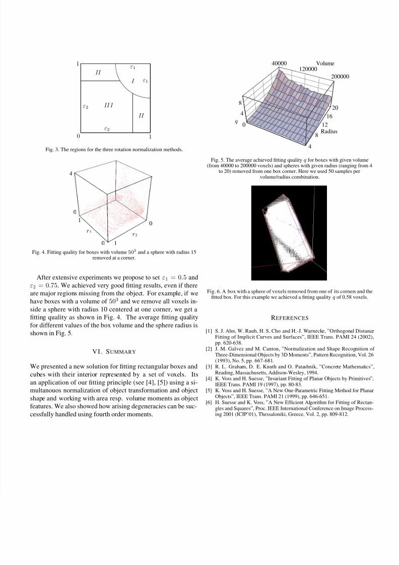
for different values of the box volume and the sphere radius is

shown in Fig. 5.

V I . SUMMARY

We presented a new solution for fitting rectangular boxes and

cubes with their interior represented by a set of voxels. Its

an application of our fitting principle (see [4], [5]) using a si-

multanouos normalization of object transformation and object

shape and working with area resp. volume moments as object

features. We also showed how arising degeneracies can be suc-

cessfully handled using fourth order moments.

8

4

0

40000120000

200000

Volume

20

16

12

8

4

Radius

q

Fig. 5. The average achieved fitting quality q for boxes with given volume(from 40000 to 200000 voxels) and spheres with given radius (ranging from 4

to 20) removed from one box corner. Here we used 50 samples pervolume/radius combination.

Fig. 6. A box with a sphere of voxels removed from one of its corners and the

fitted box. For this example we achieved a fitting quality q of 0.58 voxels.

REFERENCES

[1] S. J. Ahn, W. Rauh, H. S. Cho and H.-J. Warnecke, ”Orthogonal DistanceFitting of Implicit Curves and Surfaces”, IEEE Trans. PAMI 24 (2002),pp. 620-638.

[2] J. M. Galvez and M. Canton, ”Normalization and Shape Recognition of Three-Dimensional Objects by 3D Moments”, Pattern Recognition, Vol. 26(1993), No. 5, pp. 667-681.

[3] R. L. Graham, D. E. Knuth and O. Patashnik, ”Concrete Mathematics”,Reading, Massachusetts, Addison-Wesley, 1994.

[4] K. Voss and H. Suesse, ”Invariant Fitting of Planar Objects by Primitives”,IEEE Trans. PAMI 19 (1997), pp. 80-83.

[5] K. Voss and H. Suesse, ”A New One-Parametric Fitting Method for Planar

Objects”, IEEE Trans. PAMI 21 (1999), pp. 646-651.[6] H. Suesse and K. Voss, ”A New Efficient Algorithm for Fitting of Rectan-

gles and Squares”, Proc. IEEE International Conference on Image Process-ing 2001 (ICIP’01), Thessaloniki, Greece, Vol. 2, pp. 809-812.

Documents

A New Efficient Algorithm for Fitting Rectangular