A Hierarchical Genetic Algorithm for System Identification and Curve Fitting with a

Supercomputer Implementation

Mehmet Gulsen and Alice E. Smith1

Department of Industrial Engineering

1031 Benedum Hall

University of Pittsburgh

Pittsburgh, PA 15261 USA

412-624-5045

412-624-9831 (fax)

aesmith@engrng.pitt.edu

To Appear in IMA Volumes in Mathematics and its Applications - Issue on Evolutionary Computation (Springer-Verlag)

Editors: Lawrence Davis, Kenneth DeJong, Michael Vose and Darrell Whitley

1998

1 Corresponding author.

A Hierarchical Genetic Algorithm for System Identification and Curve Fitting with a

Supercomputer Implementation

Abstract

This paper describes a hierarchical genetic algorithm (GA) framework for identifying closed form functions for multi-variate data sets. The hierarchy begins with an upper GA that searches for appropriate functional forms given a user defined set of primitives and the candidate independent variables. Each functional form is encoded as a tree structure, where variables, coefficients and functional primitives are linked. The functional forms are sent to the second part of the hierarchy, the lower GA, that optimizes the coefficients of the function according to the data set and the chosen error metric. To avoid undue complication of the functional form identified by the upper GA, a penalty function is used in the calculation of fitness. Because of the computational effort required for this sequential optimization of each candidate function, the system has been implemented on a Cray supercomputer. The GA code was vectorized for parallel processing of 128 array elements, which greatly speeded the calculation of fitness. The system is demonstrated on five data sets from the literature. It is shown that this hierarchical GA framework identifies functions which file the data extremely well, are reasonable in functional form, and interpolate and extrapolate well.

1. INTRODUCTION

In the broadest definition, system identification and curve fitting refer to the process of selecting

an analytical expression that represents the relationship between input and output variables of a

data set consisting of iid observations of independent variables (x1, x2, ... , xn) and one dependent

variable (y). The process involves three main decision steps: (1) selecting a pool of independent

variables which are potentially related to the output, (2) selecting an analytical expression,

usually a closed form function, and (3) optimizing the parameters of the selected analytical

expression according to an error metric (e.g., minimization of sum of squared errors).

1

In most approaches, closed form functions are used to express the relationship among the

variables, although the newer method of neural networks substitutes an empirical “black box” for

a function. Fitting closed form equations to data is useful for analysis and interpretation of the

observed quantities. It helps in judging the strength of the relationship between the independent

(predictor) variables and the dependent (response) variables, and enables prediction of dependent

variables for new values of independent variables. Although curve fitting problems were first

introduced almost three centuries ago [25], there is still no single methodology that can be

applied universally. This is partially due to the diversity of the problem areas, and particularly

due to the computational limitations of the various approaches that deal with only subsets of this

broad scope. Linear regression, spline fitting and autoregressive analysis are all solution

methodologies to system identification and curve fitting problems.

2. HIERARCHICAL GENETIC APPROACH

In the approach of this paper, the primary objective is to identify an appropriate functional form

and then estimate the values of the coefficients associated with the functional terms. In fact, the

entire task is a continuous optimization process in which a selected error metric is minimized. A

hierarchical approach was used to accomplish this sequentially as shown in Figure 1. The upper

genetic algorithm (GA) selects candidate functional forms using a pool of the independent

variables and user defined functional primitives. The functions are sent to the lower

(subordinate) GA which selects the coefficients of the terms of each candidate function. This

selection is an optimization task using the data set and difference between the actual and fitted y

values.

2

y x cos xSSE= − +

=9 234 2 123 0 093 4 823

0 346271 2

2. . ( . ..

)

LowerModule

UpperModule

Function andVariable Selection

Coefficient Estimation

y Cx Ccos C C x= + +1 1 2 3 4 22( )

candidatefunctions

optimizedcoefficientsforfunctions

Figure 1 Hierarchical GA Framework

GA has been applied to system identification and curve fitting by several researchers.

The relevant work on these can be categorized into two groups. The first category includes

direct adaptation of the classical GA approach to various curve fitting techniques [17, 23]. In

these works GA replaces traditional techniques as a function optimization tool. The second

category includes more comprehensive approaches where not only parameters of the model, but

the model itself, are search dimensions. One pioneering work on this area is Koza’s adaptation

of Genetic Programming (GP) to symbolic regression [18]. The idea of genetically evolving

programs was first implemented by [8, 12]. However, GP has been largely developed by Koza

who has done the most extensive study in this field [18, 19]. More recently, Angeline used the

basic GP approach enhanced with adaptive crossover operators to select functions for a time

series problem [1].

3

3. COEFFICIENT ESTIMATION (LOWER GA)

The approach consists of two independently developed modules which work in a single

framework. The lower GA works as a function call from the upper one to measure how well the

selected model fits the actual data. In the lower GA, the objective is to select functional term

coefficients which minimize the total error over the set of data points being considered. A real

value encoding is used. The next sections describe population generation, evolution, evaluation,

selection, culling and parameter selection.

3.1 The Initial Population

Using the example of the family of curves given by equation 1, there are two variables, x1 and

x2, and four coefficients. Therefore each solution (population member) has four real numbers,

C1, C2, C3, C4.

(1) y C C x C x C x x= + + +1 2 13

3 2 4 1cos 2

The initial estimates for each coefficient are generated randomly over a pre-specified range

defined for each coefficient. The specified range need not include the true value of the

coefficient (though this is beneficial). The uniform distribution is used to generate initial

coefficient values for all test problems studied in this paper, although this is not a requirement

either (see [15] for studies on diverse ranges and other distributions).

3.2 Evolution Mechanism

A fitness (objective function) value which measures how well the proposed curve fits the actual

data is calculated for each member of the population. Squared error is used here (see [15] for

4

studies on absolute error and maximum error). Minimum squared error over all data points

results in maximum fitness.

Parents are selected uniformly from the best half of the current population. This is a

stochastic form of truncation selection originally used deterministically in evolution strategies

for elitist selection (see [2] for a good discussion of selection in evolution strategies).

Mühlenbein and Schlierkamp-Voosen later used the stochastic version of truncation selection in

their Breeder Genetic Algorithm [20]. The values of the offspring’s coefficients are determined

by calculating the arithmetic mean of the corresponding coefficients of two parents. This type of

crossover is known as extended intermediate recombination withα = 0 5. [20].

For mutation, first the range for each coefficient is calculated by determining the

maximum and minimum values for that particular coefficient in the current population. Then the

perturbation value is obtained by multiplying the range with a factor. This factor is a random

variable which is uniformly distributed between ±k coefficient range. The value of k is set to 2 in

all test problems in this paper. However, the range among the population generally becomes

smaller and smaller during evolution. In order to prevent this value from becoming too small,

and thus insignificant, a perturbation limit constant, ∆ , is set. This type of mutation scheme is

related to that used in Mühlenbein and Schlierkamp-Voosen's Breeder Genetic Algorithm [20].

However their range was static where the range in this approach adapts according to the extreme

values found in the current population with a lower bound of ∆. Mutation is applied to M

members of the population, which are selected uniformly. After mutation and crossover, the

newly generated mutants and offspring are added to the population and the lowest ranked

members are culled, maintaining the original population size, ps.

5

Cycle length, cl, is used as a basis for terminating the search process. It refers to the

number of generations without any improvement in the fitness value prior to termination. If the

algorithm fails to create offspring and mutants with better fitness values during this fixed span of

generations, the search process is automatically terminated.

3.3 Parameter Selection

The lower GA was examined at various population parameters, namely population size ps,

number of mutants M, number of offspring O, perturbation limit constant and cycle length cl,

as shown in Table 1. The experimental design covered a wide range of values and a full factorial

experiment was performed.

∆

Table 1 Evolution Parameter Levels for the Lower GA

Level ps O M ∆ cl

Low 30 10 5 10-6 10

10-5 50

100

Medium

50 20 10 10-4 500

10-3 1000

2000

High 100 50 20 10-2 5000 Based on experimental test results, ps = 30, O = 10, M = 10 ∆ = 10 and cl = 100 were

selected for the lower GA. The strategy in selecting

5−

∆ and cycle length is based on selecting the

maximum value and minimum cycle length provided that the algorithm satisfies convergence

criteria for all cases. Increasing or decreasing cl reduces computational effort, but it may also

deteriorate the accuracy of the final results. An opposite strategy, decreasing or increasing cl

improves accuracy, but it will take the algorithm more effort to converge to the final results.

∆

∆

∆

6

3.4 Test Problems

Since the lower GA module was initially developed independently from the framework, it was

tested on three test problems where the correct functional form is provided. Two of these three

test problems were taken from previous GA studies on curve fitting.

The first test problem is to estimate the value of two coefficients (C1 and C2) of the

straight line given in equation 2. This was studied by [17] with their GA approach.

y C x C= +1 2 (2)

The second test problem, which is given in equation 3, has 10 independent variables and 9

coefficients to be estimated. This was studied for spline fitting using a GA by [23] and, before

that, for conventional spline fitting by [11]. A set of 200 randomly selected data points was

used, and the problem was designed so that the response depends only on the first five variables.

The remaining variables, x6 through x10, have no effect on the response function, and they are

included in the data set as misleading noise. Therefore the optimal values of C5 through C9

should be zero.

(3) y C x x C x C x C x C xnn

n= + − + + + −=∑1 1 2 2 3

23 4 4 5 1

6

10

0 5sin( ) ( . )π

The third test problem is a general second level equation of three variables. The function, which

is given in equation 4, has 10 coefficients to be estimated, and it is larger and more complex than

any that can be found in the previous literature on using genetic algorithms for coefficient

estimation.

(4) y C C x C x C x C x C x C x C x x C x x C x x= + + + + + + + + +1 2 1 3 2 4 3 5 12

6 22

7 32

8 1 2 9 1 3 10 2 3

7

The performance of the lower GA was tested with respect to data set size, population

distribution and interval for sampling, error metric, initial coefficient range and random seeds.

Robust performance was observed for all of the above parameters and performance exceeded

previous approaches in terms of minimization of error (for details see [15]). The lower GA is

highly flexible, and it can be adopted to different problem instances and parameters with very

minor modifications in the algorithm. The coefficient optimization module is used as a

subroutine to the function identification module described in the next section.

4. FUNCTIONAL FORM SELECTION (UPPER GA)

Although the desire to develop a heuristic method to select the functional form was expressed in

the literature as early as 1950s, it was suggested as a possible extension of variable selection in

stepwise regression [7, 9, 28]. In the approach of this paper, a very liberal selection procedure is

used so that the search domain is open to all possible functional forms, but can also be restricted

by the user.

4.1 Encoding

In terms of GA parlance, each member of the population set is a closed form function. Since the

elements of the population are not simple numeric values, a binary array representation is not

applicable. Instead, a tree structure is used to represent each closed form function. As an

example, the tree structure for the candidate solution given below (equation 5) is illustrated in

figure 2.

(5) y x x= + + − +3 2 7 5 1 6 4 1 4 613

2. . . cos( . ) . x x1 2

The nodes in a tree structure can be categorized into two groups according to the number of

outgoing branches: the “terminal node” is the last node in each branch without any outgoing

8

branches. The nodes between the first and terminal nodes are called “intermediate nodes”, and

they have at least one outgoing branch. Each intermediate node has an operand (e.g., sin, cos,

exp, ln, +, ×) and the terminal node carries a variable or a constant. The numbers beside nodes

in figure 2 are real valued coefficients (obtained from the lower GA).

+

+

*

*

1

x1 x1

x1

+

*

x1

cos

x2

3.2

1.0 3.0

2.5

1.6

-4.1 9.2 0.5

Figure 2 Tree Structure Representation of Equation 5

Each tree structure has a starting node where branching is initiated. The number of

branches originating from a node is determined probabilistically, restricted to 0, 1 or 2. The only

exception is the first node where there must be at least one branch in order to initiate the

generation of the tree structure. The branches connecting the nodes also determine the “parent-

offspring relation” between the nodes. For a branch coming out of node a and going into node b,

node a is named the parent of node b. In a similar manner, node b is called a child of node a.

Each parent node can have one or two child nodes. It is also possible that the parent may not

have a child. If a node has two children, they are respectively called the left-child and the right-

child. However, if a node has only one child, it is still called the left-child.

9

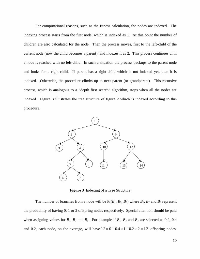
For computational reasons, such as the fitness calculation, the nodes are indexed. The

indexing process starts from the first node, which is indexed as 1. At this point the number of

children are also calculated for the node. Then the process moves, first to the left-child of the

current node (now the child becomes a parent), and indexes it as 2. This process continues until

a node is reached with no left-child. In such a situation the process backups to the parent node

and looks for a right-child. If parent has a right-child which is not indexed yet, then it is

indexed. Otherwise, the procedure climbs up to next parent (or grandparent). This recursive

process, which is analogous to a “depth first search” algorithm, stops when all the nodes are

indexed. Figure 3 illustrates the tree structure of figure 2 which is indexed according to this

procedure.

1

2

3 4

5

6 7

8

9

10

11

12

13 14

Figure 3 Indexing of a Tree Structure

The number of branches from a node will be Pr(B1, B2, B3) where B1, B2 and B3 represent

the probability of having 0, 1 or 2 offspring nodes respectively. Special attention should be paid

when assigning values for B1, B2 and B3. For example if B1, B2 and B3 are selected as 0.2, 0.4

and 0.2, each node, on the average, will have 0 2 0 0 1 0 2 2 12. .4 . .× + × + × = offspring nodes.

10

With such a number for the mean number of offspring nodes, it is possible to have tree structures

with less than 10 or 15 nodes. However, it is also possible that tree structures which have tens or

hundreds of nodes will be created. To remedy this, B1, B2 could be increased and B3 decreased.

However, this will create deep structures which will reduce the efficiency of representing the

functional forms. As a remedy, the values of B1, B2 and B3 change during the course of

branching. At the early stages, there is a higher probability for double branching which

diminishes gradually as the number of nodes increase. This is done by choosing a factor,δ , that

is equal to 0.04 × index number. The δ value is added to B1, and it is subtracted from B3 at each

node. As the number of nodes becomes larger, the probability of double branching decreases

with respect to the probability of no branching.

One dimensional arrays were used to store the tree structures. The following information

is stored for each node: (1) index number, (2) number of offspring nodes, (3) index number of

left child node, (4) index number of right child node, (5) index number of parent node, (6) type

of functional primitive assigned to the node, and (7) whether the node carries a coefficient or not.

4.2 Functional Primitives

The functional primitives are categorized into three hierarchical groups. The lowest level

includes the independent variables of the data set and the constant 1. These are assigned only to

terminal nodes and all carry a coefficient. If the variable x is assigned to a node and has

coefficient value of 4.3, then it corresponds to 4.3x. Similarly, a node with constant 1 and

coefficient -2.3 corresponds to -2.3×1 = -2.3. The second and third groups include unary and

binary operators respectively. While operators such as sin, cos, ln, exp, are categorized as

second group operators, multiplication “×”, division “÷”, and addition “+” operators form the

third group (table 2). Functional primitives can be customized by the user according to

11

estimated characteristics of closed form representation and the desired restrictiveness of the

search.

The assignment of primitives to the nodes is carried out in the following manner: the

Table 2 Node Primitives

Levels Primitives*

first group elements xn and the constant 1 are assigned to terminal nodes where there is no

outgoing branch. The unary operators are assigned to nodes with a single outgoing branch and

the binary operators are assigned to nodes with two outgoing branches. Each of the first and

second group operators is proceeded by a coefficient. The third group operators do not have a

coefficient preceding them, because they simply combine two sub-functions which already have

coefficients.

First Group x1,...,xn, 1

Second Group (unary) p, ln sin, cos, ex

Third Group (binary) +, ×, ÷

*n is t ent s in the data set

4.3 Initial Populati

reated in three stages. In the first stage, the tree structure is

he number of independ variable

on and Fitness

The initial population is randomly c

developed for each member of the population. At the second stage, appropriate primitives are

assigned to the nodes in a random manner. After the functional form representation is obtained

for the initial population, the fitness value of each member is calculated. The coefficient

estimation process is done by the subordinate GA program, which is used as a function call in

the main program. Two metrics are used for fitness: the first one is the raw fitness, which is the

sum of squared errors. The second fitness value is developed to penalize complex functional

representations in order to prevent overfitting. This secondary fitness value, called “penalized

12

fitness”, is calculated by worsening the raw fitness in proportion to the complexity of the closed

form function.

The complexity of a closed form function is determined by the number of nodes it has.

However complexity is not a absolute concept and the user needs to judge the level of

complexity for each data set. The objective is to balance the bias and variance in a closed form

representation, where bias results from smoothing out the relationship and variance indicates

dependence of the functional form on the exact data sample used [14]. Ideally, both bias and

variance will be small. A penalty function with user tunable parameters is used to balance bias

and variance of the functional form in the GA approach.

The penalty is determined by dividing the number of nodes in the tree structure by a

threshold, T, and then taking the ( )P th power of the quotient (equation 6), where 0<P<1. T

corresponds to the minimum number of nodes in an unpenalized tree structure. In this paper T =

5 was used, thus every tree structure was subject to some level of penalty if there were more than

5 nodes. Conservatively, a small value of T can be used safely while letting P impose the

severity level of the penalty. A sample calculation for penalized fitness is presented in table 3.

P

(6) Penalized Fitness Raw Fitness Number of Nodes= × ⎛

⎝⎜⎞⎠⎟T

13

Table 3 Penalized Fitness

Raw Fitness 9.78

Number of Nodes 12

T 5

P 0.4

Complexity Coefficient

125

10 4

⎛⎝⎜

⎞⎠⎟ =

..4193

Penalized Fitness 1.4193 × 9.78 = 13.88

4.4 Evolution Mechanism

The evolution mechanism is carried out through crossover and mutation. In each generation, O

offspring and M mutants are generated. Selection for crossover and mutation, the culling process

and algorithm termination are done as in the lower GA.

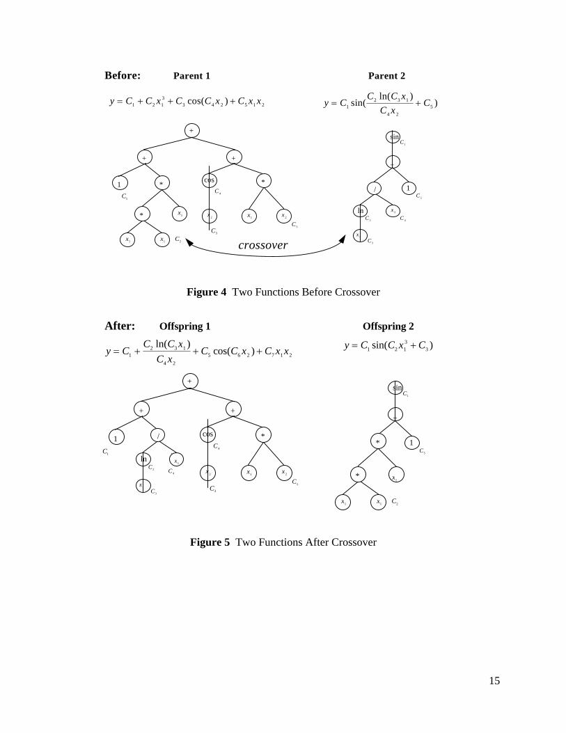
Crossover is carried out by swapping sub-branches of two members at randomly selected

nodes (figures 4 and 5). Each crossover process produces two offspring. Mutation is performed

by replacing a sub-branch (selected at any node randomly) with a new randomly generated one.

One solution could produce more than one mutant provided that branching is performed at

different nodes. The new branch used for replacement is a full function (like a member of the

initial population) but smaller in size (figures 6 and 7).

14

C 5

y C C x C C x C x x= + + +1 2 13

3 4 2 5 1 2cos( ) y CC C x

C xC= +1

2 3 1

4 25sin(

ln( ))

C5

x 2

+

+

*

*

1

x1 x1

C1

x1

C2

+

*

x1

cos

x 2

C3

C 4

C 3

+

/

x 2

x 1

1

sinC1

C 2 C 4

ln

crossover

Before: Parent 1 Parent 2

Figure 4 Two Functions Before Crossover

C5

C5

x 2

+

+

1C1

+

*

x1

cos

x 2

C3

C4

+

1

sinC1

y C C x C= +1 2 13

3sin( )y CC C x

C xC C x C x x= + + +1

2 3 1

4 25 6 2 7 1 2

ln( )cos( )

After: Offspring 1 Offspring 2

x1

*

*

x1 x1 C2

x1

C3

x 2

C4

/

x1

C2

ln x1

Figure 5 Two Functions After Crossover

15

y C C x C C x C x x= + + +1 2 13

3 4 2 5 1 2cos( )

C5

x2

+

+

*

*

1

x1 x1

C1

x1

C2

+

*

x1

cos

x2

C3

C4

mutation

Before:

C3

x1

+

x1

C1

C2

exp

x2

Parent 1

Figure 6 Function Before Mutation

+

+

*

*

1

x 1 x 1

C 1

x 1

C 2

+

*

x 1

c o s

x 2

C 3

C 4

C 7

x 1

+

x 1

C 5

C 6

e x p

y C C x C C x C x C x C x= + + + +1 2 13

3 4 2 5 1 6 1 7 12c o s ( ) e x p ( )

A f t e r : M u t a n t

Figure 7 Function After Mutation

4.5 Parameter Setting

The experiments on the upper GA were performed using the selected parameters of the lower

GA held constant and a cycle length of 100 generations for the upper GA. Since the algorithm

converged to sufficiently accurate results for all population parameter combinations tested

16

(Table 4), the population parameters were selected only on the basis of computational efficiency

(total number of fitness calculations performed during the search process). Based on this

criterion, ps = 30, O = 10, and M = 20 were selected for the upper GA. The penalty severity

factor P was harder to choose. A low value enables better fit as measured by the sum of the

squared errors (SSE) but encourages more complex functions. A high value has the opposite

effect. In the test problems, small data sets were run with P = 0.40 and larger data sets were run

at both P = 0.05 and P = 0.40. However, the user will probably want to run the GA at several

values of P and compare the resulting error and functional forms.

Table 4 Evolution Parameter Levels for the Lower GA

Level ps O M P

Low 30 10 20 0.05

0.10

Medium

50 20 40 0.20

0.40

High 100 50 60 0.80

5. COMPUTATIONAL CONSIDERATIONS

The framework includes two sequential search algorithms (the upper and lower GAs). For each

closed form representation, the coefficients are determined by running a secondary search

routine. In a similar manner, for each set of coefficient values, an error metric is calculated over

the data points. The computational requirement expands exponentially from top to the bottom

(figure 8).

17

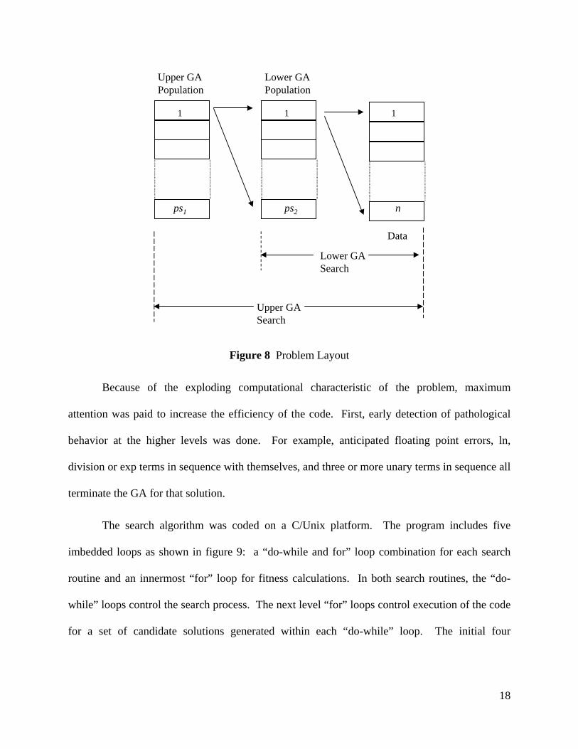
Lower GASearch

Data

ps1 ps2 n

111

Upper GASearch

Upper GAPopulation

Lower GAPopulation

Figure 8 Problem Layout

Because of the exploding computational characteristic of the problem, maximum

attention was paid to increase the efficiency of the code. First, early detection of pathological

behavior at the higher levels was done. For example, anticipated floating point errors, ln,

division or exp terms in sequence with themselves, and three or more unary terms in sequence all

terminate the GA for that solution.

The search algorithm was coded on a C/Unix platform. The program includes five

imbedded loops as shown in figure 9: a “do-while and for” loop combination for each search

routine and an innermost “for” loop for fitness calculations. In both search routines, the “do-

while” loops control the search process. The next level “for” loops control execution of the code

for a set of candidate solutions generated within each “do-while” loop. The initial four

18

imbedded loops are highly “fragile” with several control mechanisms which may skip loop

execution for some cases or even break the loop.

do { create O crossovers and M mutants for(i=0; i<O+M) do { create O1 crossovers and M1 mutants for(i=0; i<O2+M2) for(i=0; i<ndata) fitness calculation } while (lower GA search criteria is not satisfied); } while (upper GA search criteria is not satisfied);

Figure 9 Pseudo-code for Search Algorithm.

Test problems 1, 2 and 5 were done on Sun/SPARC™ workstations. For test problems 3

and 4, the program was run on a Cray C90™ supercomputer. In order to use the “vectorization”

utility, the innermost loop, where the error metric (fitness) is calculated over the data set, was

reorganized to eliminate all data dependencies. The vector size was 128, which means 128

operations when calculating fitness can be done in parallel. With a fully vectorized innermost

loop the program’s flop rate ranged between 170 Mflops to 350 Mflops, depending on the data

set size.

6. EMPIRICAL DATA SETS

In order to evaluate the effectiveness of the GA framework, five benchmark problems from the

literature were studied. The size of the test problems ranges from single variable/50 observations

to 13 variables/1000 observations. Each of the five test problems addresses a specific issue in

the curve fitting field. The first two problems are classic examples from the nonlinear regression

literature. The third test problem is sunspot data, which is one of the benchmark problems in

time series analysis. The fourth test problem includes 13 variables and approximately 1000

19

observations. This data set was originally used for neural network modeling of a ceramic slip

casting process. The last problem with 5 variables was studied earlier for qualitative fuzzy

modeling and system identification using neural networks.

The GA was run five times for each penalty factor with different random number seeds.

For test problems 1 and 2 only one penalty factor, 0.4, was used. For test problems 3 through 5,

two penalty factors, 0.4 and 0.05, were used. As expected with the higher penalty factor, the

algorithm converged to more compact functions. When the penalty was relaxed, the final closed

form representations became more complex, but with better fitness values.

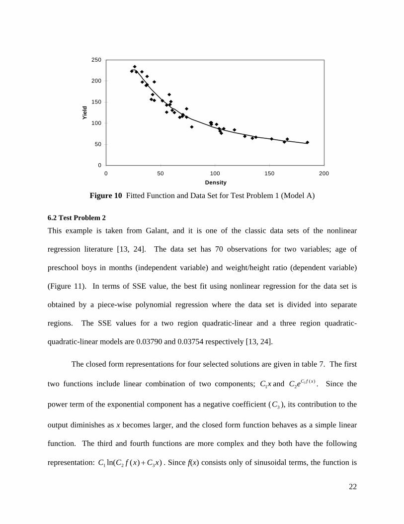
6.1 Test Problem 1

This example is taken from Nash [21], and it is one of the classic data sets of nonlinear

regression that has been studied by many researchers. The data gives the growth of White

Imperial Spanish Onions at Purnong Landing. It includes only one independent variable, density

of plants (plants/meter squared), and a dependent variable, yield per plant. For the data set, Nash

cites three potential models for the relationship between the independent variable, x (density),

and the dependent variable, y (yield):

Bleasdale and Nelder [4]: (7) y b b x b= + −( ) /1 2

1 3

Holliday [16]: (8) y b b b x= + + −( )1 2 32 1

Farazdaghi and Harris [10]: (9) y b b x b= + −( )1 213

Since density figures are in the order of hundreds and power terms are present in the models, the

parameters are logarithmically scaled. Determination of model parameters of the above

equations was based on minimizing a natural logarithm error metric.

The GA used the data directly, not in the logarithmic form. Using a penalty factor = 0.4,

four runs were selected for further examination. As can be seen from the listing in table 5, the

20

simplest closed form function has two imbedded logarithmic terms divided by the independent

variable, x. The second representation is more complex than the first one, and it has an

exponential term with a compound power argument. The third and fourth functions are complex

versions of the second and first functions respectively. Apart from the first closed form function,

all equations have sinusoidal components. Since the actual data is not cyclic in nature, presence

of such terms implies overfitting the data. The plot of the first function is presented in figure 10.

The comparison of SSE values of the GA models with respect to those cited by Nash is given in

table 6. In order to establish a common base for comparison, SSE values were recalculated for

the four GA models after a logarithmic transformation. Although the error metric for fitness

calculation was different than those used in the models cited by Nash [21], all of the GA models

gave superior results in terms of logarithmic SSE values.

Table 5 Selected Closed Form Functions for Test Problem 1

Model Equation SSE

A xx))/0.0597n(33.7043(2190.3680l 5065.244

B )))8.7108+)cos(0.9751n(-35.8300n(-0.3734l(-2.8443si17.6377exp xx

4021.240

C )))4.7735+6x))sin(12.331os(-5.2830n(-28.811cn(-0.3957l(-3.0512si12.6422exp x

3651.378

D )0.0833+5.6118/ /(3

)))61sin(182.59os(-1.0273(116.0904c176.2871lnxx

x 3388.789

Table 6 Comparison of Results for Test Problem 1

Model SSE Bleasdale-Nelder 0. 2833 Holliday 0. 2842 Farazdaghi-Harris 0. 2829 Model A 0. 276 Model B 0. 238 Model C 0. 216 Model D 0. 214

21

0

50

100

150

200

250

0 50 100 150 200Density

Yiel

d

Figure 10 Fitted Function and Data Set for Test Problem 1 (Model A)

6.2 Test Problem 2

This example is taken from Galant, and it is one of the classic data sets of the nonlinear

regression literature [13, 24]. The data set has 70 observations for two variables; age of

preschool boys in months (independent variable) and weight/height ratio (dependent variable)

(Figure 11). In terms of SSE value, the best fit using nonlinear regression for the data set is

obtained by a piece-wise polynomial regression where the data set is divided into separate

regions. The SSE values for a two region quadratic-linear and a three region quadratic-

quadratic-linear models are 0.03790 and 0.03754 respectively [13, 24].

The closed form representations for four selected solutions are given in table 7. The first

two functions include linear combination of two components; and . Since the

power term of the exponential component has a negative coefficient ( ), its contribution to the

output diminishes as x becomes larger, and the closed form function behaves as a simple linear

function. The third and fourth functions are more complex and they both have the following

representation: . Since f(x) consists only of sinusoidal terms, the function is

xC1)(

23 xfCeC

3C

))(ln( 321 xCxfCC +

22

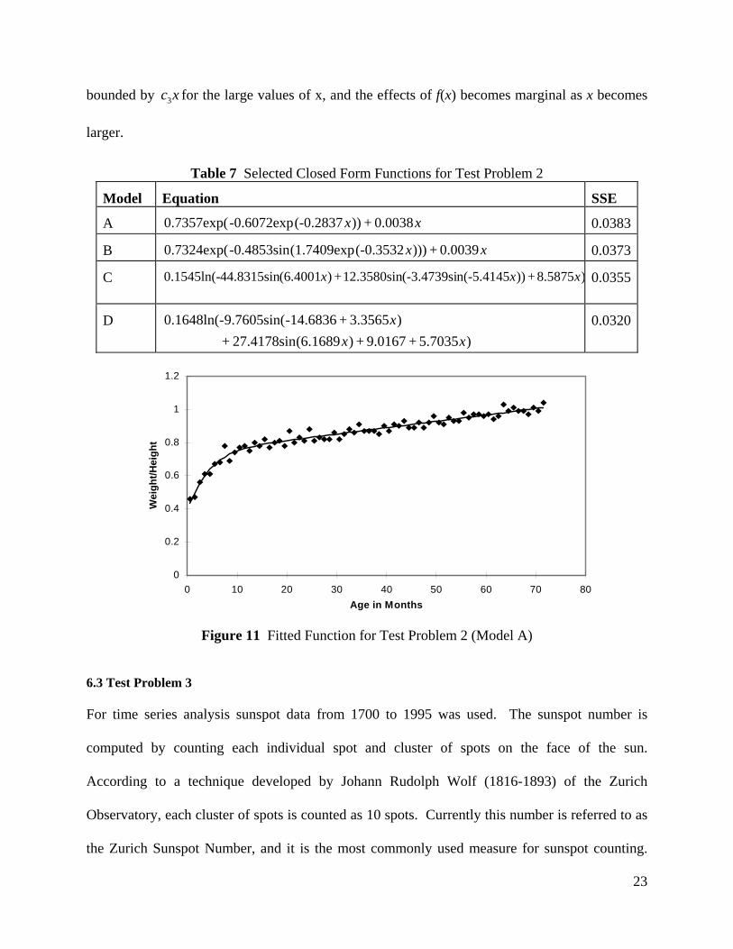
bounded by for the large values of x, and the effects of f(x) becomes marginal as x becomes

larger.

c x3

Table 7 Selected Closed Form Functions for Test Problem 2

Model Equation SSE

A xx 0.0038+))(-0.2837-0.6072exp0.7357exp( 0.0383

B xx 0.0039+)))(-0.3532(1.7409exp-0.4853sin0.7324exp( 0.0373

C )8.5875+))n(-5.4145(-3.4739si12.3580sin+)(6.400144.8315sin0.1545ln(- xxx

0.0355

D )5.7035+9.0167+)(6.168927.4178sin+

)3.3565+-14.68369.7605sin(0.1648ln(-xx

x

0.0320

0

0.2

0.4

0.6

0.8

1

1.2

0 10 20 30 40 50 60 70 80Age in Months

Wei

ght/H

eigh

t

Figure 11 Fitted Function for Test Problem 2 (Model A)

6.3 Test Problem 3

For time series analysis sunspot data from 1700 to 1995 was used. The sunspot number is

computed by counting each individual spot and cluster of spots on the face of the sun.

According to a technique developed by Johann Rudolph Wolf (1816-1893) of the Zurich

Observatory, each cluster of spots is counted as 10 spots. Currently this number is referred to as

the Zurich Sunspot Number, and it is the most commonly used measure for sunspot counting.

23

Since results vary according to interpretation of the observer and the atmospheric conditions

above the observation site, an international number is computed by averaging the measurements

of 25 cooperating observatories throughout the world.2 The data is highly cyclic with peak and

bottom values approximately in every 11.1 years. However, the cycle is not symmetric, and the

number of counts reaches a maximum value faster than it drops to a minimum.

The original data which had only one input and the output value (time (t) and sunspot

number Y(t)) was reorganized to include 15 additional input variables, sunspot numbers Y(t-15)

to Y(t-1) (equation 10). The observations start from 1715 and the first observation includes the

following variables: time (t=15) and 15 sunspots numbers from 1700 to 1714. The data was

divided into two groups. The first 265 observations (until 1979) were used to develop the

models. In order to evaluate the model performance beyond the training data, sunspot data from

1980 to 1995 was used.

Y t f t Y t Y t Y t( ) ( , ( ), ( ), . . . . . , ( ))= − − −1 2 15 (10)

Table 8 Selected Closed Form Functions for Test Problem 3.

Model Equation SSE

A 9)-0.2471(+2)-0.4585(-1)-1.1965( ttt 61964

B 2))-0.6271(-1))-p(-0.3263((-2.7260ex15.7476exp+

9))--0.3512(1.1989exp(-1)-0.8337(tt

tt

45533

C 9)-0.1148(+4)-0.1316(-1)-0.8064(+1)-2))(-0.8446(-

1))-0.4282(+4)-(1.4097(-0.6099cos1.2410exp(ttttt

tt

40341

2 For more information about sunspots and computation techniques see the homepage of the National Oceanic and Atmospheric Administration at http://www.ngdc.noaa.gov.stp.SOLAR.SSN.ssn.html.

24

D

9)-0.1046(+4)-0.1413(-1)-0.8253(+1)-2)(-0.9362(-2))-0.7485(-2))-3.1756(-2))-2.8807(+

4))-(0.2561(-3.3442cos0.6979exp(+4)-(-1.4893(-0.5564cos1.6258exp(

tttttttt

tt

38715

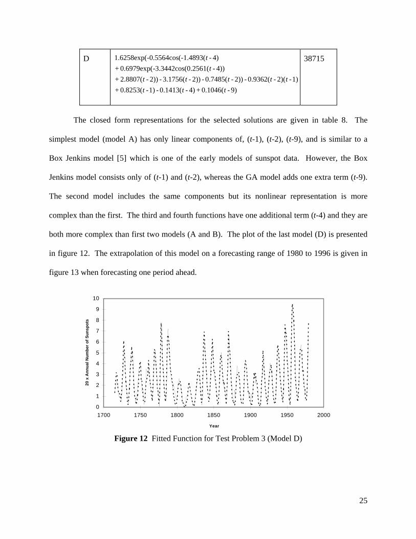
The closed form representations for the selected solutions are given in table 8. The

simplest model (model A) has only linear components of, (t-1), (t-2), (t-9), and is similar to a

Box Jenkins model [5] which is one of the early models of sunspot data. However, the Box

Jenkins model consists only of (t-1) and (t-2), whereas the GA model adds one extra term (t-9).

The second model includes the same components but its nonlinear representation is more

complex than the first. The third and fourth functions have one additional term (t-4) and they are

both more complex than first two models (A and B). The plot of the last model (D) is presented

in figure 12. The extrapolation of this model on a forecasting range of 1980 to 1996 is given in

figure 13 when forecasting one period ahead.

0

1

2

3

4

5

6

7

8

9

10

1700 1750 1800 1850 1900 1950 2000

Year

20 x

Ann

ual N

umbe

r of S

unsp

ots

Figure 12 Fitted Function for Test Problem 3 (Model D)

25

0

1

2

3

4

5

6

7

8

9

1980 1985 1990 1995Ye a r

Figure 13 Extrapolation of Models Beyond Training Data Range

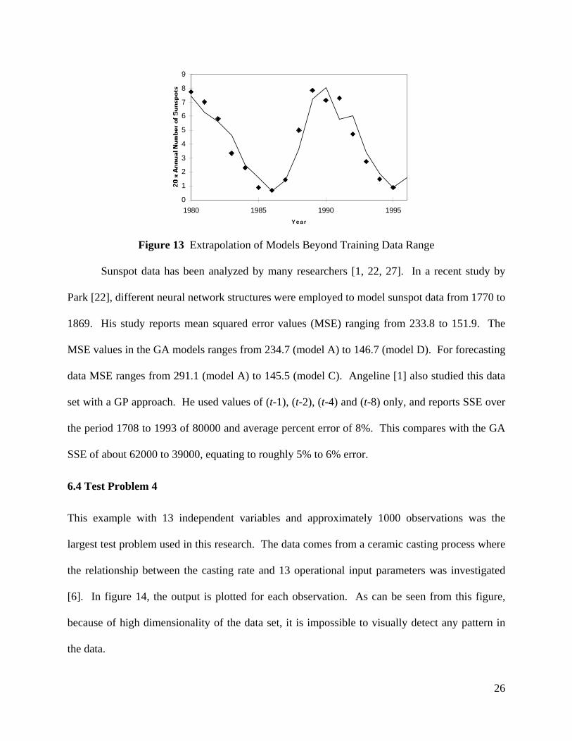
Sunspot data has been analyzed by many researchers [1, 22, 27]. In a recent study by

Park [22], different neural network structures were employed to model sunspot data from 1770 to

1869. His study reports mean squared error values (MSE) ranging from 233.8 to 151.9. The

MSE values in the GA models ranges from 234.7 (model A) to 146.7 (model D). For forecasting

data MSE ranges from 291.1 (model A) to 145.5 (model C). Angeline [1] also studied this data

set with a GP approach. He used values of (t-1), (t-2), (t-4) and (t-8) only, and reports SSE over

the period 1708 to 1993 of 80000 and average percent error of 8%. This compares with the GA

SSE of about 62000 to 39000, equating to roughly 5% to 6% error.

6.4 Test Problem 4

This example with 13 independent variables and approximately 1000 observations was the

largest test problem used in this research. The data comes from a ceramic casting process where

the relationship between the casting rate and 13 operational input parameters was investigated

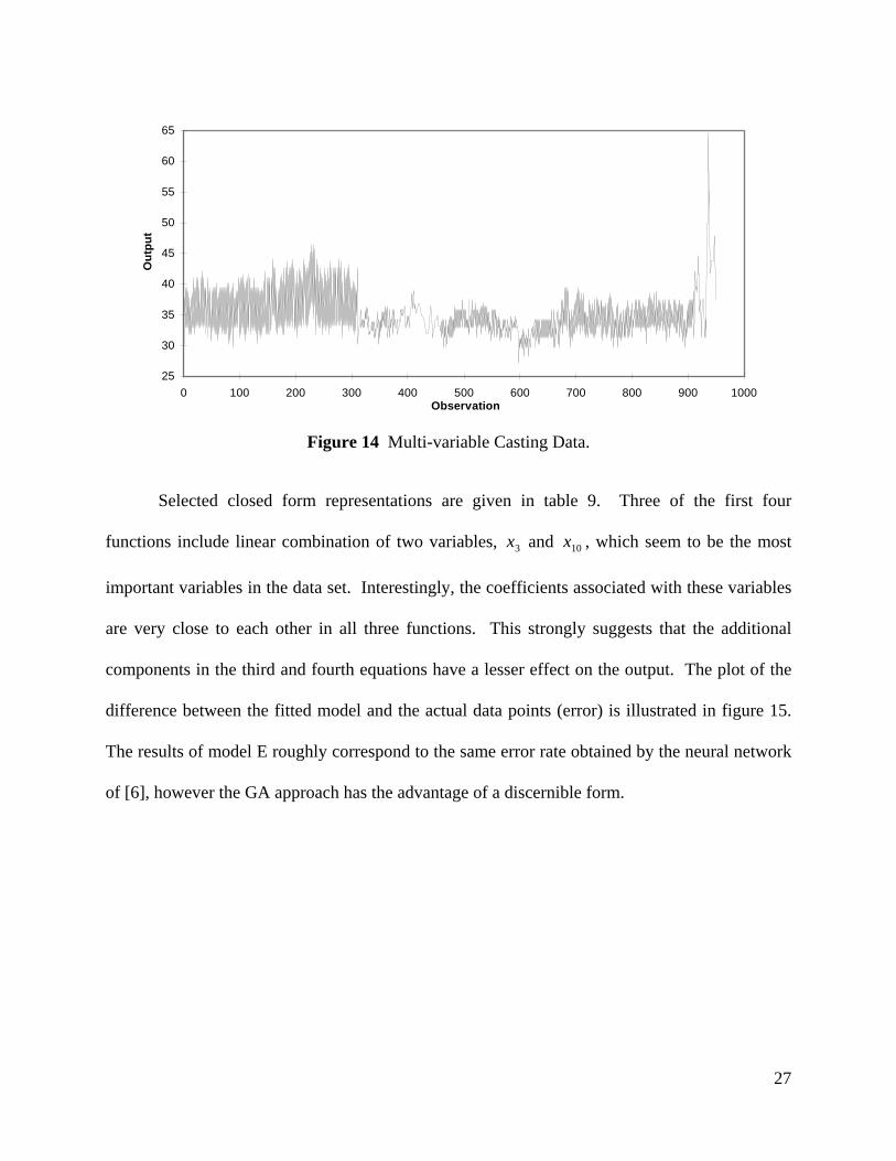
[6]. In figure 14, the output is plotted for each observation. As can be seen from this figure,

because of high dimensionality of the data set, it is impossible to visually detect any pattern in

the data.

26

25

30

35

40

45

50

55

60

65

0 100 200 300 400 500 600 700 800 900 1000Observation

Out

put

Figure 14 Multi-variable Casting Data.

Selected closed form representations are given in table 9. Three of the first four

functions include linear combination of two variables, and , which seem to be the most

important variables in the data set. Interestingly, the coefficients associated with these variables

are very close to each other in all three functions. This strongly suggests that the additional

components in the third and fourth equations have a lesser effect on the output. The plot of the

difference between the fitted model and the actual data points (error) is illustrated in figure 15.

The results of model E roughly correspond to the same error rate obtained by the neural network

of [6], however the GA approach has the advantage of a discernible form.

x3 x10

27

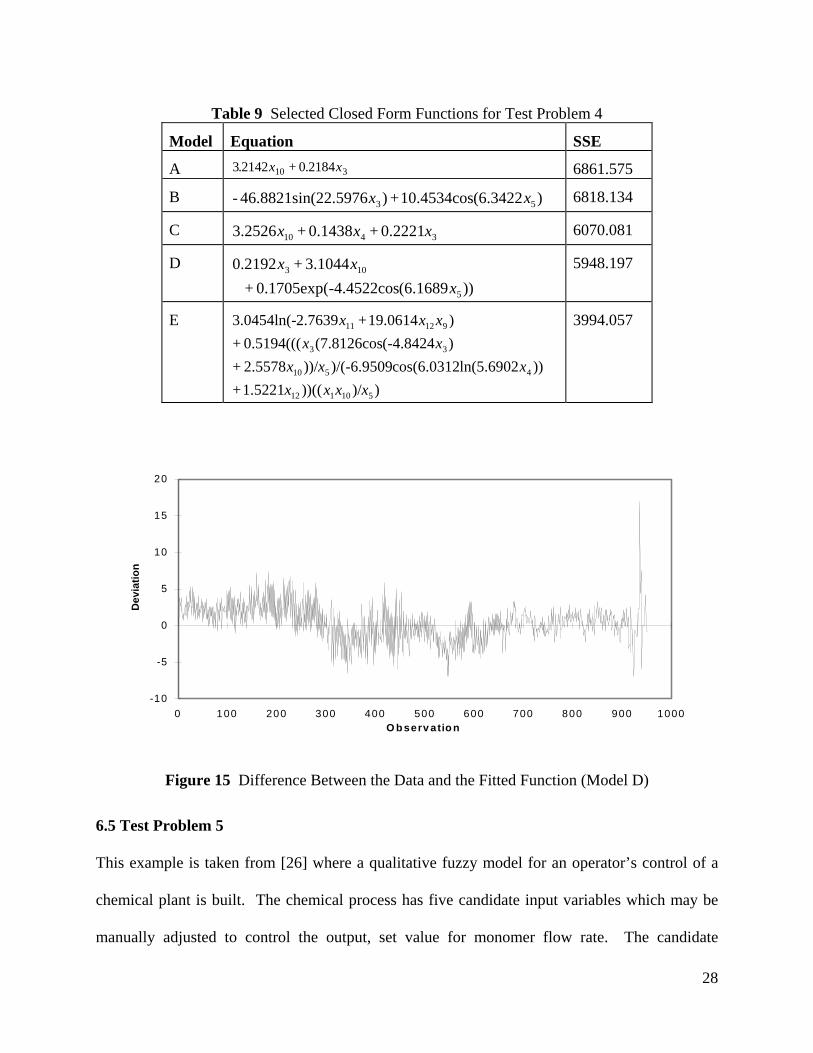
Table 9 Selected Closed Form Functions for Test Problem 4

Model Equation SSE

A 3 2142 0 218410 3. + .x x 6861.575

B )(6.342210.4534cos+)(22.597646.8821sin- 53 xx 6818.134

C 3410 0.2221+0.1438+3.2526 xxx 6070.081

D ))(6.1689-4.4522cos0.1705exp(+

3.1044+0.2192

5

103

xxx

5948.197

E

))/))((1.5221+))ln(5.6902cos(6.0312)/(-6.9509))/2.5578+

)(-4.8424(7.8126cos0.5194(((+)19.0614+2.76393.0454ln(-

510112

4510

33

91211

xxxxxxx

xxxxx

3994.057

-10

-5

0

5

10

15

20

0 100 200 300 400 500 600 700 800 900 1000O b serv atio n

Dev

iatio

n

Figure 15 Difference Between the Data and the Fitted Function (Model D)

6.5 Test Problem 5

This example is taken from [26] where a qualitative fuzzy model for an operator’s control of a

chemical plant is built. The chemical process has five candidate input variables which may be

manually adjusted to control the output, set value for monomer flow rate. The candidate

28

variables are (1) monomer concentration (x1), (2) change of concentration (x2), (3) actual

monomer flow rate (x3), (4) temperature 1 inside the plant (x4) and (5) temperature 2 inside the

plant (x5). The data set includes 70 observations of the above six variables (figure 16). The

authors first generated six data clusters by using fuzzy clustering and identified x1, x2 and x3 as

the most relevant parameters.

The same data set was also studied by [3]. Their neural network model identified x3 as

the single most significant input parameter followed by x1. Their model also includes x5, which

has a very marginal effect on the accuracy of the model.

Table 10 Selected Closed Form Functions for Test Problem 5

Model Equation SSE

A 33 0.9694+))(0.8913-0.9109sin0.1877exp( xx 0.6057

B 33 0.9903+))))n(1.0549(-3.8097si(3.2885exp-0.8714cos0.2033exp(- xx

0.3864

C

33

125

0.8915+)-0.89690.2013sin(+ 2.3442-)0.2486+2.0012x1.8257cos(

xxxx

0.3553

D

333

335

1.046464+)1.5718+ ))-3.02622.7400sin(-8cos(-5.8207.98470.0505sin(

xxxxxx

0.3321

E

3

335

3

0.9968+ ))0.4712+ )6.9550-3.0451+3.8175+3.35751.8731sin(-

)2.7229-(1.6935(3.0478cos-1.4083sin0.1318exp(

xxxx

x

0.2753

There are some similarities between the GA results and the previous research. All five

solutions given in table 10 contain a linear component of x3, which was identified as the most

significant parameter by both [3] and [26]. This shows that there is one to one relationship

between x3 and the output. In the actual system, the output is the set point value for monomer

flow rate, and x3 represents the actual flow rate. Thus, such a relationship between these two

29

parameters could be anticipated. The exponential term with a negative coefficient of three of the

functions reflects that the deviation between the output and x3 is diminishing in later

observations. Although there is not any information about the data collection procedure, the

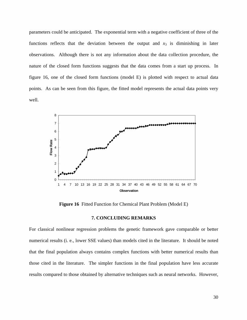
nature of the closed form functions suggests that the data comes from a start up process. In

figure 16, one of the closed form functions (model E) is plotted with respect to actual data

points. As can be seen from this figure, the fitted model represents the actual data points very

well.

0

1

2

3

4

5

6

7

8

1 4 7 10 13 16 19 22 25 28 31 34 37 40 43 46 49 52 55 58 61 64 67 70

Observation

Flow

Rat

e

Figure 16 Fitted Function for Chemical Plant Problem (Model E)

7. CONCLUDING REMARKS

For classical nonlinear regression problems the genetic framework gave comparable or better

numerical results (i. e., lower SSE values) than models cited in the literature. It should be noted

that the final population always contains complex functions with better numerical results than

those cited in the literature. The simpler functions in the final population have less accurate

results compared to those obtained by alternative techniques such as neural networks. However,

30

unlike neural networks, this approach provides a function which can be used directly for both

intuitive analysis and mathematical computation.

One distinguishing feature of this approach is that it gives a set of solutions to the user.

The user can study those solutions and choose the model that satisfies both complexity and

numerical accuracy constraints. The user can also review the set of good functions for similarity

in terms (independent variables and primitive functions) so that the relationship can be better

understood. Furthermore, it is very easy for the user to specify different penalty severities,

different sets of primitives, and different error metrics to explore the variety of functions, their

form and fit with the data. This distinguishes the hierarchical GA framework as an effective

global approach for system identification and curve fitting. The only significant drawback is the

magnitude of computational effort required. However, since system identification and curve

fitting are usually done infrequently and off-line, there is no imperative for extreme

computational speed.

ACKNOWLEDGEMENT

Alice E. Smith gratefully acknowledges the support of the U.S. National Science Foundation

CAREER grant DMI 95-02134.

31

REFERENCES

[1] Angeline, Peter J., “Two self-adaptive crossover operators for genetic programming,” Advances in Genetic Programming Volume II (editors: Peter J. Angeline and Kenneth E. Kinnear, Jr.), MIT Press, Cambridge MA, 89-109, 1996.

[2] Bäck, T. and Schwefel, H. P., “An overview of evolutionary algorithms for parameter optimization,” Evolutionary Computation, 1, 1-23, 1993.

[3] Bastian, A. and Gasos, J., “A type I structure identification approach using feed forward neural networks,” IEEE International Conference on Neural Networks, 5 (of 7), 3256-3260, 1994.

[4] Bleasdale, J. K. A. and Nelder, J. A., “Plant population and crop yield,” Nature, 188, 342, 1960.

[5] Box, G. E. and Jenkins, G. M., Time Series Analysis: Forecasting and Control, Holden-Day, San Francisco, CA, 1970.

[6] Coit, D. W. and Jackson-Turner, B. and Smith, A. E., “Static neural network process models: considerations and case studies,” International Journal of Production Research, forthcoming.

[7] Collins, J. S., “A regression analysis program incorporating heuristic term selection,” Machine Intelligence, Donald Michie Editor, American Elsevier Company, New York NY, 1968.

[8] Cramer, N. L., “A representation for the adaptive generation of simple sequential programs,” Proceedings of an International Conference on Genetic Algorithm and Their Applications, 183-187, 1985.

[9] Dallemand, J. E., “Stepwise regression program on the IBM 704,” Technical Report of General Motors Research Laboratories, 1958.

[10] Farazdaghi, H. and Harris, P. M., “Plant competition and crop yield,” Nature, 217, 289-290, 1968.

[11] Friedman, J., “Multivariate adaptive regression splines,” Department of Statistics Technical Report 102, Stanford University, 1988 (revised 1990).

[12] Fujiko, C. and Dickinson, J., “Using the genetic algorithm to generate LISP source code to solve prisoner’s dilemma,” Genetic Algorithms and Their Applications: Proceedings of the Second International Conference on Genetic Algorithms, 236-240, 1987.

[13] Gallant, A. R., Nonlinear Statistical Models, John Wiley and Sons, New York, 1987.

[14] Geman S. and Bienenstock, E., “Neural networks and the bias/variance dilemma,” Neural Computation, 4, 1-58, 1992.

32

[15] Gulsen, M., Smith, A. E. and Tate, D. M., “Genetic algorithm approach to curve fitting,” International Journal of Production Research, 33, 1911-1923, 1995.

[16] Holliday, R., “Plant population and crop yield,” Field Crop Abstracts, 13, 159-167, 247-254, 1960.

[17] Karr, C. L., Stanley D. A., and Scheiner B. J., “Genetic algorithm applied to least squares curve fitting,” U.S. Bureau of Mines Report of Investigations 9339, 1991.

[18] Koza, J. R., Genetic Programming: On the Programming of Computers by Means of Natural Selection, MIT Press, Cambridge MA, 162-169, 1992.

[19] Koza, J. R., Genetic Programming: Automatic Discovery of Reusable Programs, MIT Press, Cambridge MA, 1994.

[20] Mühlenbein, H. and Schlierkamp-Voosen, D., “Predictive models for the breeder genetic algorithm. I. Continuous parameter optimization,” Evolutionary Computation, 1, 25-49, 1993.

[21] Nash, J. C. and Walker-Smith, M., Nonlinear Parameter Estimation: An Integrated System in BASIC, Marcel Dekker, New York, 1987.

[22] Park, Young R. and Murray, Thomas J. and Chen, Chung, “Predicting sun spots using a layered perceptron neural network,” IEEE Transactions on Neural Networks, 7, 501-505, 1996.

[23] Rogers, D., “G/SPLINES: “A hybrid of Friedman’s multivariate adaptive regression splines (MARS) algorithms with Holland’s genetic algorithm,” Proceedings of the Fourth International Conference on Genetic Algorithms, 384-391, 1991.

[24] Seber, G. A. F. and Wild, C. J., Nonlinear Regression, John Wiley and Sons, New York, 1989.

[25] Stigler, S. M. History of Statistics: The Measurement of Uncertainty Before 1900, Harvard University Press, Cambridge MA, 1986.

[26] Sugeno, M., and Yasukawa, T. “A fuzzy-logic-based approach to qualitative modeling,” IEEE Transactions on Fuzzy Systems, 1, 7-31, 1993.

[27] Villareal, J. and Baffes, P., “Sunspot prediction using neural networks,” University of Alabama Neural Network Workshop Report, 1990.

[28] Westervelt, F., Automatic System Simulation Programming, unpublished Ph.D. Dissertation, University of Michigan, 1960.

33