Evaluation of Circle Fitting Algorithm for Coordinate Measuring Machineserialsjournals.com/serialjournalmanager/pdf/1331529715.pdf · Evaluation of Circle Fitting Algorithm for Coordinate

Evaluation of Circle Fitting Algorithm for Coordinate Measuring MachineF F

39

Evaluation of Circle Fitting Algorithm forCoordinate Measuring Machine

Vijay Pandey and Ashish JaganiBirla Institute of Technology, Mesra (RANCHI).

ABSTRACT: The least-squares fitting minimize the squares sum oferror-of-fit in predefined measures. By the geometric fitting, the errordistances are defined with the orthogonal, or shortest, distances fromthe given points to the geometric feature to be fitted. For the geometricfitting of circle/sphere/ellipse/hyperbola/parabola, simple and robustnonparametric algorithms are proposed. These are based on the coord-inate description of the corresponding point on the geometric featurefor the given point, where the connecting line of the two points is theshortest path from the given point to the geometric feature to be fitted.This paper provides an overview of the state of the art in measuringthe basic entities with CMM, algorithm used to create base dimensionand CMM inspection data analysis technology. We expect that theinformation included in this review will benefit CMM softwaredevelopers, CMM users, and researchers of new CMM technology.This document is the results of a survey of published theories andpost-inspection data analysis algorithms. Principles on which currentnational and international standards are based have been stated. Thesealgorithms are commonly used in mechanical design and partinspection. The effects of using different measuring criteria arediscussed. From this theory and algorithm review, we recommenddirections for future development in these areas.Keywords: Coordinate measuring machine, curve fitting, least squaremethod.

1. INTRODUCTIONIn all aspect of everyday life we come across some sort of measuringprocedure, although in most cases we are hardly aware of it: whetherwe are reading speedometer, filling up petrol, or weighing vegetables.

International Journal of Material Research, Electronics and Electrical SystemsJanuary-December 2011, Volume 4, Number 1-2, pp. 39– 57

International Journal of Material Research, Electronics and Electrical SystemsF F

40

Apart from these very familiar activities, the term measurementencompasses with which public at large is not familiar. One of thisis Coordinate Metrology.

Coordinate metrology has now become firmly established inIndustrial Production. Today hardly a work piece exist whosedimensions can not be measured with a Coordinate MeasuringMachine.

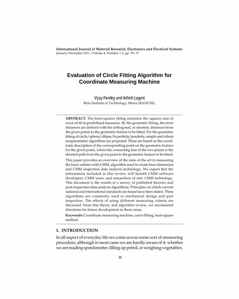
The classical measuring methods using gauges, vernier calipers,micrometers, height gauges are more and more replaced bycoordinate metrology.

Figure 1

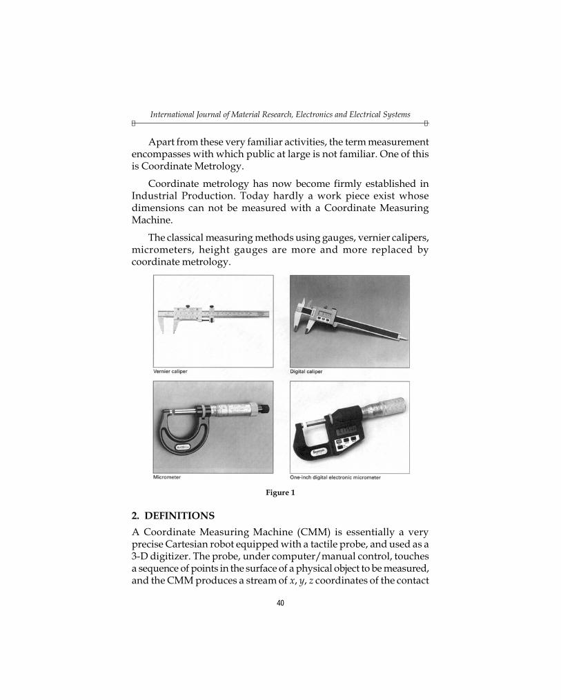
2. DEFINITIONSA Coordinate Measuring Machine (CMM) is essentially a veryprecise Cartesian robot equipped with a tactile probe, and used as a3-D digitizer. The probe, under computer/manual control, touchesa sequence of points in the surface of a physical object to be measured,and the CMM produces a stream of x, y, z coordinates of the contact


41

points. The coordinate stream is interpreted by algorithms thatsupport applications such as reverse engineering, quality control,and process control. In quality and process control, the goal is todecide if a manufactured object meets its design specifications. Thistask is called dimensional inspection, and amounts to comparingthe measurements obtained by a CMM with a solid model of theobject.

Figure 2

CMM is not object dependent and can be widely used on anytype of object. CMM can be fully automated and the output couldeasily be linked to a CAD system. CMM is comprised of fourcomponents: The machine itself, the measuring probe, the computersystem, and the computer software.

3. LITERATURE SURVEYA CMM does not directly measure geometric features such asdistances, angles or diameters. Instead it measures the coordinatesof a set of points on the surface of an artefact and then combinesthem to evaluate the desired geometric feature. So unlike Verniercalipers which directly measures the diameter of a cylinder, a CMMmeasurement requires some processing of the combination ofmeasured values to produce an estimate of the diameter. Clearly


42

then, the outputs from a CMM measurement will depend on theway in which this processing is performed (the algorithm), and theproperties of the points chosen to sample the surface of the artefact.In this report we discuss how the probing strategy used to samplethe artefact’s surface affect the results of a CMM measurement, andhow the measurement uncertainty is a powerful tool for reflectingthis.

Mathematical software, particularly curve and surface fittingroutines, is a critical component of coordinate metrology systems.An important but difficult task is to assess the performance of suchroutines. The National Institute of Standards and Technology hasdeveloped a software package, the NIST Algorithm Testing System(ATS), that can assist in assessing the performance of geometry-fitting routines. This system has been aiding in the development ofa U.S. standard (American Society of Mechanical Engineers (ASME)B89.4.10) for software performance evaluation of coordinatemeasuring systems. The ATS is also the basis of NIST’s AlgorithmTesting and Evaluation Program for Coordinate Measuring Systems(ATEP-CMS). The ATS incorporates three core modules: a datagenerator for defining and generating test data sets, a collection ofreference algorithms which provides a performance baseline for fittingalgorithms, and a comparator for analyzing the results of fittingalgorithms versus the reference algorithms.

Fitting circles and ellipses to given points in the plane is aproblem that arises in many application areas, e.g. computergraphics, coordinate metrology, petroleum engineering, statistics.In the past, algorithms have been given which fit circles and ellipsesin some least squares sense without minimizing the geometricdistance to the given points. Walter Gander presents severalalgorithms which compute the ellipse for which the sum of the squaresof the distances to the given points is minimal. These algorithms arecompared with classical simple and iterative methods. Circles andellipses may be represented algebraically i.e. by an equation of theform F(x) = 0. If a point is on the curve then its coordinates x are azero of the function F. Alternatively, curves may be represented inparametric form, which is well suited for minimizing the sum ofthe squares of the distances.


43

3.1. Algorithm Adopted by NISTThe purpose of data fitting is to apply an appropriate algorithm tofit a perfect geometric form (line, plane, circle, ellipse, cylinder,sphere, cone, etc.) to sampled data points obtained from theinspection of a manufactured part. The perfect form approximationobtained through fitting is called a substitute feature. The substitutefeature is represented by a shape vector b2. (The exact nature of bvaries with the geometric form being fit.) The substitute feature is aone-dimensional curve or a two-dimensional surface that wedesignate as a function f (u; b) of a parameter vector u. The values off are points in space (or on a surface, if fitting is being done in twodimensions). As u varies, f moves along the geometry representedby b; as b varies, the surface changes shape and location. A particulargeometry need not have a single representation. In fact, much ofthe research on fitting techniques is based on developing cleverrepresentations for curves and surfaces. The fitting problem,generally stated, is to minimize some objective function with respectto b. For some kinds of fitting (to be described below) the minimi-zation may be subject to certain constraints. The most frequentlyused fitting algorithms are based on the Lp norm. [2]

NIST has adopted following method for curve fitting.

Plane Fittingx — a point on the plane.a — the direction cosines of the normal to the plane.

Distance Equationdi = d(xi) = d(xi, x, a) = a.(xi . x)

Objective FunctionJ(x, a) = Σ[a.(xi . x)]2

Line Fittingx— a point on the line.a — the direction cosines of the line.

Distance Equationd(xi) = d(xi, x, a) = |a x (xi . x)|


44

Objective Function

J(x, a) = Σ|ax (xi . x)|2

Sphere Fitting

x — the center of the sphere.

r — the radius of the sphere.

Distance Equation

d(xi) = |xi – x| – r

Objective Function

J(x, r) = Σ(|xi – x| – r)2

Two-Dimensional Circle Fitting

x — the x -coordinate of the centre of the circle.

y — the y -coordinate of the centre of the circle.

r — the radius of the circle.

Distance Equation

d(xi, yi) = 2( – ) –iy y r+2( – )ix x

Objective Function

J(x, y, r) = Σ ( )22( – ) –iy y r+2( – )ix x

Three-Dimensional Circle Fitting

x — the center of the circle.

A — the direction numbers of the normal to circle’s plane.

r — the radius of the circle.

Distance Equation

d(xi) = 2 2( – )i ig f r+

Objective Function

J(x, A, r) = Σ(g1i + ( fi – r)2)


45

Cylinder Fittingx — a point on the cylinder axis.A — the direction numbers of the cylinder axis.r — the radius of the cylinder.

Distance Equationd(xi) = fi – r

Objective FunctionJ(x, A, r) = Σ(fi – r)2

Cone Fittingx— a point on the cone axis (not the apex).A — the direction numbers of the cone axis (pointing toward

the apex).s — the orthogonal distance from the point, x, to the cone.c — the cone’s apex semi-angle.

Distance Equationd(xi) = fi cos ψ + gi sin ψ – s

Objective FunctionJ(x, A, s, ψ) = Σ(fi cos ψ + gi sin ψ – s)2

Above algorithms have been implemented in the ATS and havebeen used for 5 years by NIST and by members of the ASME B89.4.10Working Group. They have successfully solved a number of difficultfitting problems that could not be solved by many commercialsoftware packages used on Coordinate Measuring Systems (CMSs).The ATS algorithms have an extremely broad range of convergence.Failure to converge has only been observed for pathological fittingproblems (e.g., fitting a circle to collinear points). Special checkscan detect most of these situations. The ATS algorithms are generallyrobust. For most fits, a good starting guess is not required to reachthe global minimum. This is due, in part, to the careful choice of fittingparameters, the use of certain constraints, and, for cylinders and cones,the technique of restarting a search after an initial solution is found.


46

4. DEVELOPMENT OF ALGORITHMThis report assumes that readers has some knowledge of LinearAlgebra and curve fitting. The least square best-fit reference elementto Cartesian data points was only established in this report.

4.1. Least Squares Best Fit MethodThe application of least square criteria can be applied to a wide rangeof curve fitting problems. Least square best-fit element to data isexplained by taking the problem of fitting the data to a plane.This is a problem of parameterization. The best plane can bespecified by a point C(xo, yo, zo) on the plane and the direction cosines(a, b, c) of the normal to the plane. Any point (x, y, z) on the planesatisfies.

a(x – xo) + b(y – yo) + c(z – zo) = 0

The distance from any point A(xi, yi, zi) to a plane specified aboveis given by

di = a(xi – xo) + b(yi – yo) + c(zi – zo)

The sum of squares of distances of each point from the plane is

F = 2

1

n

ii

d=∑

Hence our problem is to find the parameters (xo, yo, zo) and (a, b, c)that minimizes the sum F.

4.2. OptimizationConsider a function

E(u) = 2

1

( )n

ii

d u=∑

which has to be minimized with respect to the parameters

u = (u1 ... un)T

Here in this case di represents the distance of the data point tothe geometric element parameterized by u.


47

4.3. Linear Least SquaresThe conventional approach used in the standard textbooks for leastsquare fitting of a straight line is described below for the under-standing. The matrix formulation of the problem is also explainedin detail, as it is very useful when solving large problems. Considerfitting a straight line

y = a + bxthrough a set of data points (xi, yi) i = 1 to n. The minimizing

function minimizes the sum of the squares of the distances of thepoints from the straight line measured in the vertical direction. Thus

F = 2

1

( – – )n

i ii

y a bx=∑

is the minimizing function. A necessary condition for F to beminimum is

F

a

∂∂

= 0 andF

b

∂∂

= 0

Thus partial differentiation of the above function with respectto a and b gives

2(–1)1

( – – )n

i ii

y a bx=∑ = 0

2(–xi)1

( – – )n

i ii

y a bx=∑ = 0

These can be simplified as

1 1

n n

i ii i

y na b x= =

= +∑ ∑

2

1 1 1

–n n n

i i i ii i i

x y a x b x= = =

=∑ ∑ ∑

Solving above equations simultaneously, which give us thevalues for a and b.


48

4.4. Normal EquationConsider to fit a straight line, y = a + bx, to the set of data (x1, y1),(x2, y2), ..., (xn, yn). If the data points were collinear, the line wouldpass through n point.

So, y1 = a + bx1

y2 = a + bx2

y3 = a + bx3

::

yn = a + bxn

It can be written in a matrix form

1

2

n

y

y

y

=

1

2

1

1

1 n

x

x

x

a

b

Let B =

1

2

n

y

y

y

. A =

1

2

1

1

1 n

x

x

x

. and p =a

b

So it can be compacted as B = AP

The objective is to find a vector p that minimizes the Euclideanlength of the difference ||B – AP||.

if P = P* =*

*

a

b

is a minimize vector, y = a* + b*x is a least square

straight-line fit. This can be explained as

||B – AP||2 = (y1 – a – bx1)2 + (y2 – a – bx2)2 + … + (yn – a – bxn)2

if let d1 = (y1 – a – bx1)2, d2 = (y2 – a – bx2)2, … , dn = (yn – a – bxn)2

d can be explained as the distance from a point of a data set to afitting line. So

||B – AP||2 = d12 + d2

2 + d32 + ... + dn

2


49

To minimize ||B – AP||, AP must be equal to AP* where AP* isthe orthogonal projection of B on the column space of A. This impliesB – AP* must be orthogonal to the column space of A. So

(B – AP*)AP = 0for every vector P in R2

This can be written as

(AP)T (B – AP*) = 0PTAT (B – AP*) = 0

PT (ATB – ATAP*) = 0(ATB – ATAP*)P = 0

So ATB – ATAP* is orthogonal to every vector P in R2. This implies

ATB – ATAP* = 0

ATAP = ATB

Which implies that P* satisfies the linear sys

ATAP = ATB

This equation is called as Normal equation. This will providethe solution for p

P = (ATA)–1 ATBThis equation can be used in the case of least square fit of a

polynomial.

4.5. Gauss-Newton AlgorithmNewton’s method is one of the most powerful and well-knownnumerical methods for solving a root finding problem f(x) = 0, wheref(x) is a non-linear function. This technique is used in applicationsof linear least squares model of circle, sphere, cylinder, and cones.To motivate how such an algorithm works, first the Newton methodis described.

Suppose that given a function f that its domain is [a, b], and let x∈ [a, b] such that f’(x) ≠ 0. The Taylor polynomial expansion for f(x)about x is


50

f(x) = f( x ) + (x – x ) f’(x) +2( – )

2

x x f’(ξ(x))

where ξ(x) ∈[ x, x ].

since f(q) = 0 where q = x, it gives

0 = f(x) + ( x – x) f’( x ) +2( – )

2

x x f’(ξ(x))

Newton’s method is assumed as |q – x | is small. Therefore(q – x)2 is much small. So

0 = f( x ) + (q – x ) f’( x )

(q – x ) = – ( )

'( )

f x

f x

Let q = u1, x = u0, and p = –( )

'( )

f x

f x

Therefore u1 = u0 + p and p = – 0

0

( )

' ( )

f u

f u

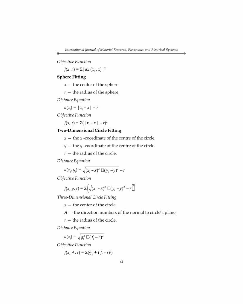
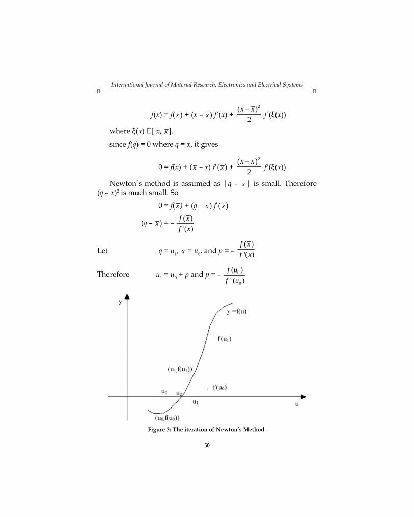
Figure 3: The iteration of Newton’s Method.


51

The iteration of Newton’s method

From figure the root finding problem y = f(u) can be done byfollowing steps:

(1) f(u0) and f’(u0) are evaluated.(2) A tangent line to graph at the point (u0, f(u0)) is found.

It cuts the u axis at u1.(3) Find point u1, and draw a tangent to graph at the point u1 to

find point u2.(4) These steps above are repeated until it is converged (close

to u*).The main ingredients of the algorithm are

(a) given an approximate solution, the problem is linearised.(b) the linear version of the problem is solved.(c) the solution of the linear problem is used to update estimate

of the solution.In the linear least square problem, the measurement of how well

the geometric element fits a set of data point can be determined

E = 2

1

n

ii

d=

∑Where di is a distance from the point to the geometric element.

In the case, di is not linear function; the Gauss-Newton algorithm isused for finding the minimum of a sum of squares E. Assuming thereis one initial estimate u*, solve a linear least squares system of the form

Jp = –dWhere J is the m × n Jacobean matrix whose ith row is the gradient

of di with respect to the parameter u, i.e.,

Jij = i

j

d

u

∂∂

It’s evaluated at u, and the ith component of d is di(u). Theparameter is updated as

u = u + p


52

4.6. Converged ConditionsSteps of Newton’s algorithm are repeated until it reaches to aconvergent point. Here 3 criteria are relevant for testing forconvergence:

(1) the change of E should be small.(2) the size of the update, for instance (pTp)½, must be small.(3) the partial derivation of E with respect to the optimization

parameters, for instance (ggT)½where g = JTd, should be small.

4.7. Least Square Fitting of Basic Elements: CircleThe procedure to fit a circle to m data points (xi, yi), where m ≥ 3, isgiven below. Any point (x, y) on the circle satisfies

(xi – xo)2 + (yi – yo)2 = r2

It is known that the distance from a point (xi, yi) to a circlespecified by xo, yo, and r and is given by,

di = ri – rwhere ri = [(xi – xo)2 + (yi – yo)2]½

and the elements of the Jacobean matrix J are found from thepartial derivative of di with respect to the parameter xo, yo and r isgiven by

0

id

x

∂∂

= –(xi – x0)/ri

0

id

y

∂∂

= –(yi – y0)/ri

id

r

∂∂

= – 1

A circle can be specified by a center (xo, yo) and a radius r.

The algorithm that is used to find the best-fit circle is Gauss-Newton algorithm. First the initial estimates are to be found thenthe Gauss-Newton algorithm is implemented. The initial estimatesof the center and radius of the circle are made by solving the problemas a linear least square model. The steps that are followed are as follows:


53

(i) Minimization of F

F = 2

1

n

ii

f=∑

Where fi = ri2 – r2

(ii) This can be reduced to a linear system in x0, y0 and ρ as,fi = (xi – x0)2 + (yi – y0)2 – r2

= –2xi x0 – 2yi y0 + ρ + (xi2 + yi

2)where ρ is xo

2 + yo2 – r2

(iii) For minimizing F, the linear least squares system is solvedA[x0 y0 ρ]T = b;

where the elements of the ith row of A are the coefficients (2xi,2yi, –1) and the ith element of b is xi

2 + yi2.

(iv) An estimate of r is obtained from the equation of ρ.Once the initial estimates are obtained the right hand side vector

d and Jacobean matrix J are formed. Then the linear least-squaressystem is solved.

J[Px0 Py0 Pr ]T = –d ;The values of the parameters are updated according to the

estimates

xo = xo + pxo, yo = yo + pyo, r = r + pr.The above steps are repeated until the algorithm converges.

5. VALIDATION

5.1. Modeling the CMM MeasurementThe measured points and their uncertainties are the input parametersto the simulation model that mimics the behaviour of the CMM. Inorder for the model to produce reliable uncertainty estimates it isvital that the model processes the measured coordinates in exactlythe same way as what the CMM does. Therefore, the model mustuse exactly the same fitting algorithm as the one used by the CMMeven if a superior one exists. In most cases the fitting algorithm used


54

by the CMM is a least squares fit, where the sum of the square of thedeviation of the points from a best fitted theoretical surface isminimized.

Verification of the model is relatively straightforward as theoutputs from the model should be exactly the same as that obtainedfrom the CMM, when both use the same measured points as inputs.

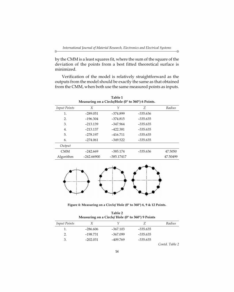
Table 1Measuring on a Circle/Hole (0° to 360°) 6 Points.

Input Points X Y Z Radius1. –289.051 –374.899 –335.6362. –196.304 –374.815 –335.6353. –213.139 –347.964 –335.6354. –213.137 –422.381 –335.6355. –278.197 –416.711 –335.6356. –274.061 –349.522 –335.635

OutputCMM –242.669 –385.174 –335.636 47.5050

Algorithm –242.66900 –385.17417 47.50499

Figure 4: Measuring on a Circle/ Hole (0° to 360°) 6, 9 & 12 Points.

Table 2Measuring on a Circle/ Hole (0° to 360°) 9 Points

Input Points X Y Z Radius1. –286.606 –367.103 –335.6352. –198.731 –367.099 –335.6353. –202.031 –409.769 –335.635

Contd. Table 2


55

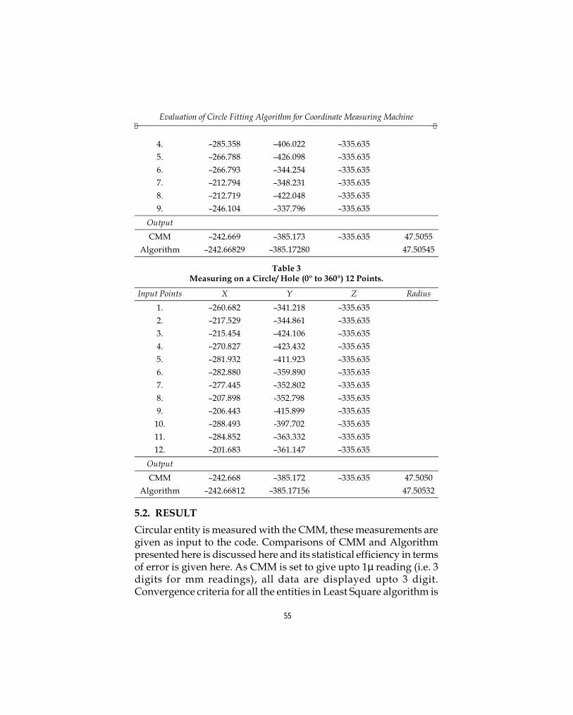
4. –285.358 –406.022 –335.6355. –266.788 –426.098 –335.6356. –266.793 –344.254 –335.6357. –212.794 –348.231 –335.6358. –212.719 –422.048 –335.6359. –246.104 –337.796 –335.635

OutputCMM –242.669 –385.173 –335.635 47.5055

Algorithm –242.66829 –385.17280 47.50545

Table 3Measuring on a Circle/ Hole (0° to 360°) 12 Points.

Input Points X Y Z Radius1. –260.682 –341.218 –335.6352. –217.529 –344.861 –335.6353. –215.454 –424.106 –335.6354. –270.827 –423.432 –335.6355. –281.932 –411.923 –335.6356. –282.880 –359.890 –335.6357. –277.445 –352.802 –335.6358. –207.898 -352.798 –335.6359. –206.443 -415.899 –335.635

10. –288.493 -397.702 –335.63511. –284.852 –363.332 –335.63512. –201.683 –361.147 –335.635

OutputCMM –242.668 –385.172 –335.635 47.5050

Algorithm –242.66812 –385.17156 47.50532

5.2. RESULTCircular entity is measured with the CMM, these measurements aregiven as input to the code. Comparisons of CMM and Algorithmpresented here is discussed here and its statistical efficiency in termsof error is given here. As CMM is set to give upto 1µ reading (i.e. 3digits for mm readings), all data are displayed upto 3 digit.Convergence criteria for all the entities in Least Square algorithm is


56

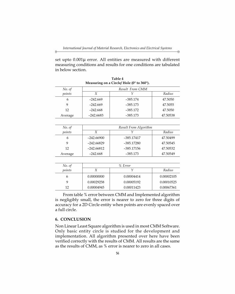
set upto 0.001µ error. All entities are measured with differentmeasuring conditions and results for one conditions are tabulatedin below section.

Table 4Measuring on a Circle/ Hole (0° to 360°).

No. of Result From CMMpoints X Y Radius

6 –242.669 –385.174 47.50509 –242.669 –385.173 47.5055

12 –242.668 –385.172 47.5050Average –242.6683 –385.173 47.50538

No. of Result From Algorithmpoints X Y Radius

6 –242.66900 –385.17417 47.504999 –242.66829 –385.17280 47.50545

12 –242.66812 –385.17156 47.50532Average –242.668 –385.173 47.50549

No. of % Errorpoints X Y Radius

6 0.00000000 0.00004414 0.000021059 0.00029258 0.00005192 0.00010525

12 0.00004945 0.00011423 0.00067361

From table % error between CMM and Implemented algorithmis negligibly small, the error is nearer to zero for three digits ofaccuracy for a 2D Circle entity when points are evenly spaced overa full circle.

6. CONCLUSIONNon Linear Least Square algorithm is used in most CMM Software.Only basic entity circle is studied for the development andimplementation. All algorithm presented over here have beenverified correctly with the results of CMM. All results are the sameas the results of CMM, as % error is nearer to zero in all cases.


57

REFERENCES[1] “A Review of Current Geometric Tolerancing Theories and Inspection Data

Analysis Algorithms”, Shaw C. Feng , Theodore H. Hopp U.S. DEPARTMENTOF COMMERCE, National Institute of Standards and Technology, February 1991.

[2] Craig M. Shakarji, “Least-Squares Fitting Algorithms of the NIST AlgorithmTesting System”, Journal of Research of the National Institute of Standards andTechnology , 103, No. 6, pp. 633-641.

[3] “Least-Squares Fitting of Circles and Ellipses”, Walter Gander, Gene H., GolubRolf Strebel.

[4] “Reverse Engineering Using Structured Lighting”, B.Tech. report, By PrabhuR. & Krishna Tunga R. Indian Institute of Technology – Madras, May 2001.

Documents

Evaluation of Circle Fitting Algorithm for Coordinate Measuring Machineserialsjournals.com/serialjournalmanager/pdf/1331529715.pdf · Evaluation of Circle Fitting Algorithm for Coordinate