Embed Size (px)
Citation preview
A New Control Strategy forCoordinated Control of GroundVehicle Vertical Dynamics via
Control Allocation
by
Michael Karl Binder
A thesispresented to the University of Waterloo
in fulfillment of thethesis requirement for the degree of
Master of Applied Sciencein
Mechanical Engineering
Waterloo, Ontario, Canada, 2014
c© Michael Karl Binder 2014

Author’s Declaration
I hereby declare that I am the sole author of this thesis. This is a true copy of the thesis,including any required final revisions, as accepted by my examiners.
I understand that my thesis may be made electronically available to the public.
ii
Abstract
The scope of this thesis concerns the basic research and development of a coordinatedcontrol system for the control of vehicle roll and pitch dynamics using suspension forces asactuators. In this thesis, the following question is explored: How can suspension control(particularly semi-active control) be generalized to control all vertical vehicle dynamics ina coordinated way, and which would ideally be integrable with modern ESC systems? Thechosen approach to this problem will be the application of the control allocation method-ology for overactuated systems, which makes use of online mathematical optimization inorder to realize the desired control law. Background information on vehicle dynamics andmodeling, suspension control, control allocation and optimization is presented along with abrief literature review. The coordinated suspension control system (CSC) is designed andsimulated. High-level controllers and control allocators are designed and their stabilityproperties are explored. Then, the focus is shifted towards implementation and experi-mentation of the coordinated control system on a real vehicle. The semi-active actuatorsare statistically modeled along with the deployed sensors. Both the hardware and soft-ware designs are explored. Finally, experiments are designed and results are discussed.Recommendations for future inquiry are given in the conclusion of this work.
iii
Acknowledgements
I would like to thank my advisor Dr. Khajepour for supporting and guiding me in thisrather expansive project. I would also like to thank Kevin Cochran and Jeff Gransmaa forlending their technical expertise, without which the experimental part of my thesis wouldhave been much more daunting. Finally, I would like to thank everyone I have met andbefriended in my time here at the lab and at the University of Waterloo for making mystay in Canada truly a pleasure.
iv

Dedication
This thesis is dedicated to my family, who always support me unconditionally in myendeavours.
v

Table of Contents
List of Tables ix
List of Figures x
1 Introduction 1
1.1 Scope . . . . . . . . . . . . . . . . . . . . . . . . . . . . . . . . . . . . . . 2
1.2 Outline . . . . . . . . . . . . . . . . . . . . . . . . . . . . . . . . . . . . . . 3
2 Background and Literature Review 4
2.1 Vehicle Dynamics and Modeling . . . . . . . . . . . . . . . . . . . . . . . . 4
2.1.1 Two-Track Vehicle Model . . . . . . . . . . . . . . . . . . . . . . . 5
2.1.2 Quarter-Car Model . . . . . . . . . . . . . . . . . . . . . . . . . . . 8
2.1.3 Half-Car and Full-Car Models . . . . . . . . . . . . . . . . . . . . . 9
2.2 Suspension Control . . . . . . . . . . . . . . . . . . . . . . . . . . . . . . . 12
2.2.1 Active Systems . . . . . . . . . . . . . . . . . . . . . . . . . . . . . 12
2.2.2 Semi-active Systems . . . . . . . . . . . . . . . . . . . . . . . . . . 13
2.3 Optimization and Control Allocation . . . . . . . . . . . . . . . . . . . . . 15
2.3.1 Control Allocation . . . . . . . . . . . . . . . . . . . . . . . . . . . 15
2.3.2 Quadratic Programming . . . . . . . . . . . . . . . . . . . . . . . . 17
vi
3 Design and Simulation 21
3.1 High-Level Controller Design . . . . . . . . . . . . . . . . . . . . . . . . . . 21
3.1.1 Roll Control . . . . . . . . . . . . . . . . . . . . . . . . . . . . . . . 21
3.1.2 Pitch and Vertical Motion Control . . . . . . . . . . . . . . . . . . 24
3.2 Control Allocator Design . . . . . . . . . . . . . . . . . . . . . . . . . . . . 25
3.2.1 Control Effectiveness Matrix . . . . . . . . . . . . . . . . . . . . . . 26
3.2.2 Active Systems . . . . . . . . . . . . . . . . . . . . . . . . . . . . . 27
3.2.3 Semi-active Systems . . . . . . . . . . . . . . . . . . . . . . . . . . 28
3.2.4 Adaptivity and Fault Tolerance . . . . . . . . . . . . . . . . . . . . 29
3.2.5 System Stability with the Control Allocator . . . . . . . . . . . . . 33
3.3 Simulation Results . . . . . . . . . . . . . . . . . . . . . . . . . . . . . . . 33
3.3.1 Active System . . . . . . . . . . . . . . . . . . . . . . . . . . . . . . 34
3.3.2 Semi-active System . . . . . . . . . . . . . . . . . . . . . . . . . . . 34
3.4 Discussion . . . . . . . . . . . . . . . . . . . . . . . . . . . . . . . . . . . . 35
4 Implementation and Experimentation 42
4.1 Instrumentation and Hardware Design . . . . . . . . . . . . . . . . . . . . 42
4.1.1 Magnetorheological Dampers . . . . . . . . . . . . . . . . . . . . . 44
4.1.2 Sensors . . . . . . . . . . . . . . . . . . . . . . . . . . . . . . . . . . 47
4.1.3 Embedded Computing with the dSPACE AutoBox . . . . . . . . . 49
4.2 Software Design . . . . . . . . . . . . . . . . . . . . . . . . . . . . . . . . . 49
4.2.1 Input Processing and Estimation . . . . . . . . . . . . . . . . . . . 50
4.2.2 High-Level Controllers . . . . . . . . . . . . . . . . . . . . . . . . . 51
4.2.3 Control Allocator . . . . . . . . . . . . . . . . . . . . . . . . . . . . 51
4.2.4 Output Processing . . . . . . . . . . . . . . . . . . . . . . . . . . . 52
4.3 Experimental Results . . . . . . . . . . . . . . . . . . . . . . . . . . . . . . 52
4.3.1 Double Lane-Changes . . . . . . . . . . . . . . . . . . . . . . . . . 52
4.3.2 Stopping Tests . . . . . . . . . . . . . . . . . . . . . . . . . . . . . 55
4.4 Discussion . . . . . . . . . . . . . . . . . . . . . . . . . . . . . . . . . . . . 57
vii
5 Conclusions and Future Work 64
5.1 Conclusions . . . . . . . . . . . . . . . . . . . . . . . . . . . . . . . . . . . 64
5.2 Recommendations for Future Work . . . . . . . . . . . . . . . . . . . . . . 64
Bibliography 67
viii
List of Tables
3.1 Quantitative measures from simulation. . . . . . . . . . . . . . . . . . . . . 41
4.1 Quantitative measures from Trial 1 of the double lane-change test. . . . . . 56
4.2 Quantitative measures from Trial 2 of the double lane-change test. . . . . . 56
4.3 Quantitative measures from Trial 1 of the stopping test. . . . . . . . . . . . 56
4.4 Quantitative measures from Trial 2 of the stopping test. . . . . . . . . . . . 56
4.5 Sample means and variances from test data. . . . . . . . . . . . . . . . . . 56
4.6 Student’s t-test results and p-values. An asterisk denotes meeting the lowconfidence threshold α = 0.1. . . . . . . . . . . . . . . . . . . . . . . . . . 61
ix
List of Figures
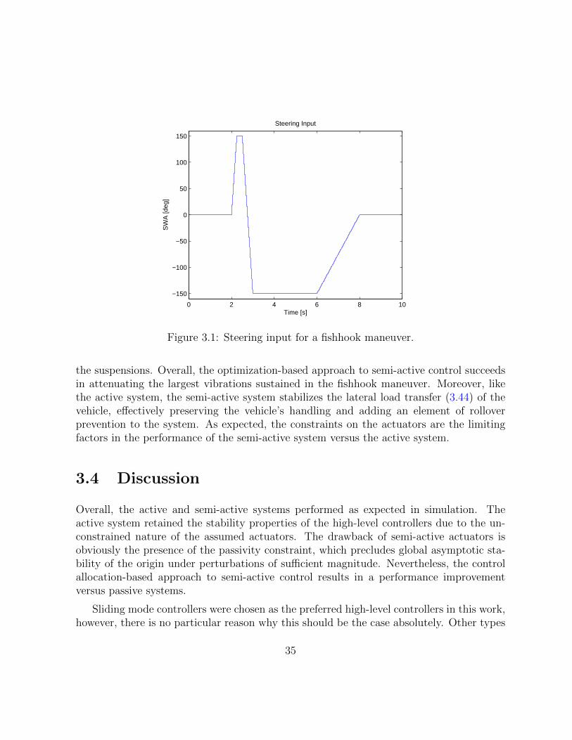
3.1 Steering input for a fishhook maneuver. . . . . . . . . . . . . . . . . . . . . 35
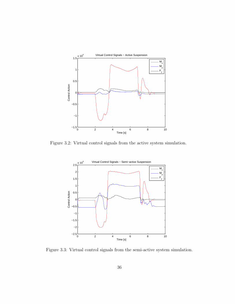
3.2 Virtual control signals from the active system simulation. . . . . . . . . . 36
3.3 Virtual control signals from the semi-active system simulation. . . . . . . . 36
3.4 Actuator control signals from the active system simulation. . . . . . . . . . 37
3.5 Actuator control signals from the semi-active system simulation. . . . . . . 37
3.6 Current input signals from the semi-active system simulation. . . . . . . . 38
3.7 Suspension velocities from the semi-active system simulation. . . . . . . . . 38
3.8 Load transfer ratio (rollover index) of the vehicle. . . . . . . . . . . . . . . 39
3.9 Plots of the vehicle’s roll response. . . . . . . . . . . . . . . . . . . . . . . 39
3.10 Plots of the vehicle’s pitch response. . . . . . . . . . . . . . . . . . . . . . . 40
3.11 Plots of the vehicle’s vertical response. . . . . . . . . . . . . . . . . . . . . 40
4.1 Cadillac STS test platform. . . . . . . . . . . . . . . . . . . . . . . . . . . 43
4.2 Basic overview of the control system instrumentation. . . . . . . . . . . . . 43
4.3 MR Damper force-velocity trajectory at specified current input. . . . . . . 45
4.4 MR Damper characteristic surface plots. . . . . . . . . . . . . . . . . . . . 46
4.5 Servo driver calibration curve. . . . . . . . . . . . . . . . . . . . . . . . . . 47
4.6 Suspension sensor calibration curves. . . . . . . . . . . . . . . . . . . . . . 48
4.7 Roll response from Trial 1 of the double lane-change test. . . . . . . . . . . 53
4.8 Roll rate response from Trial 1 of the double lane-change test. . . . . . . . 54
x
4.9 Adaptivity parameters in a double lane-change. The pitch parameter acti-vates at the end when breaking is initiated. . . . . . . . . . . . . . . . . . . 54
4.10 Speed and steering inputs in Trial 1 of the double lane-change test. . . . . 55
4.11 Calculated force outputs from the double lane-changes. . . . . . . . . . . . 57
4.12 Pitch response from Trial 1 of the stopping test. . . . . . . . . . . . . . . . 58
4.13 Pitch rate response from Trial 1 of the stopping test. . . . . . . . . . . . . 58
4.14 Adaptivity parameters in a stopping test. The pitch parameter is activethroughout the accelerating and breaking phases of the maneuver. . . . . . 59
4.15 Speed inputs in Trial 1 of the stopping test. . . . . . . . . . . . . . . . . . 59
4.16 Calculated force outputs from the stopping tests. . . . . . . . . . . . . . . 60
xi
Chapter 1
Introduction
The work presented in this thesis originated out of the ”Holistic Vehicle Control” (HVC)project in development at the Mechatronic Vehicle Systems Lab at the University of Wa-terloo and funded by General Motors Corporation (GM). The HVC project is a form ofelectronic stability control (ESC), whereby vehicle slip is controlled and yaw rate trackingis achieved using torque vectoring.
The goal of the HVC system is to compute an optimal distribution of forces at the tirecontact patches, which generate the desired yaw moment, longitudinal and lateral forces toattain the aforementioned objectives. Such a process is an example application of controlallocation, as it is referred to in the literature. What makes such a system interesting isits potential for generalization, that is, its potential to form a basis for a complete, unifiedvehicle dynamics control system, covering all elementary degrees of freedom of the vehiclesystem.
One of these degrees of freedom which maintains particular importance in achievingvehicle stability is roll. It is well known that excessive roll angle, as well as great lateralacceleration precipitates the phenomenon of vehicle rollover, which accounts for a greatmany number of annual traffic accidents in the US and elsewhere. The oft quoted figureof 9,882 deaths due to rollover in the US in the year 2000 can be found in [8]. The dangerof rollover is proportionally greater for vehicles with high centers of gravity, such as SUVs.A control system which aids in the prevention of rollover thus has great utility in regardsto vehicle safefy.
Another set of dynamics to be controlled are the pitch dynamics. Unlike with roll,controlling vehicle pitch has little to do with stability, but rather has utility in improvingvehicle economy. If the pitch dynamics can be controlled, then the dynamic longitudinal
1
load transfer can be stabilized, which normalizes the vertical loads on the tires, thus im-proving traction and minimizing wasted energy, particularly when accelerating or braking.
The means by which the control of these vertical dynamics, i.e. the roll, pitch, andpure vertical motion of a vehicle, can be handled is via the vehicle suspensions. To date,most suspension control, particularly semi-active control, is actually done in isolation fromthe overall dynamics of the vehicle. By this, we mean that suspension controllers areprincipally designed with the stabilization of the individual suspension in mind, to theexclusion of the rest of the vehicle dynamics.
In this thesis, the following question is answered: How can suspension control (partic-ularly semi-active control) be generalized to encompass all vertical vehicle dynamics in acoordinated way, and which would ideally be integrable with modern ESC systems? Ourapproach to this problem will be the application of the control allocation methodology foroveractuated systems, which like other control paradigms such as model-predictive control,makes use of online mathematical optimization in order to realize the desired control law.
1.1 Scope
The scope of this thesis concerns the basic research and development of a coordinatedcontrol system for the control of vehicle roll and pitch dynamics using suspension forcesas actuators. The control system developed herein is a new application of techniques incontrol allocation. The use of control allocation is to date unprecedented in the scope ofsemi-active suspension control, which has largely been limited to formulations designed fora single corner of the vehicle, e.g. skyhook, groundhook, and hybrid control, among others.Using control allocation, we seek to integrate the suspension controls into a framework formultiobjective vehicle control. Furthermore, though the system under study is motivated inpart by the prospect of integrating it with ESC systems, all simulation and experimentationof the control system is done without such stability systems in the loop. This is largelydue to the fact that there is not currently a vehicle test platform with both controllablesuspensions and torque vectoring (or differential braking) systems present in the lab.
This work is focused primarily on control design, simulation, and initial testing. Thougha complete vehicle dynamics control system must necessarily also possess parameter andstate estimation modules, particularly for systems to be implemented in the commercialsphere, the design of such modules will largely be excluded. For the testing of the co-ordinated control system, all values of interest can be measured or approximated frommeasurements by deployed sensors. Both the design of these modules and the task ofintegration with ESC systems provide worthwhile directions for further research.
2
In the sections on design, we will consider the cases of both active and semi-activeactuators. To date, semi-active suspensions remain the most commercially viable choicefor controllable suspensions, with fully active systems being featured on relatively fewmodels. Active systems, however, remain an area of active research and development andmight one day become the new standard. The focus of the experimental section will be onsemi-active suspensions.
1.2 Outline
The organization of this thesis proceeds as follows. In Chapter 2, background informationon vehicle dynamics and modeling, suspension control, control allocation and optimizationis presented along with a brief literature review. In Chapter 3, the coordinated suspensioncontrol system is designed and simulated. High-level controllers and control allocators aredesigned and their stability properties are explored. In Chapter 4, the focus is shiftedtowards implementation and experimentation of the coordinated control system on a realvehicle. The semi-active actuators are statistically modeled along with the deployed sen-sors. Both the hardware and software designs are explored. Finally, experiments aredesigned and results are discussed. In Chapter 5, we conclude our findings and give rec-ommendations for future inquiry.
3
Chapter 2
Background and Literature Review
2.1 Vehicle Dynamics and Modeling
A ground vehicle is a multi-body, nonlinear dynamic system. As such, vehicle dynamics canbe very complex, oftentimes more complicated than any one vehicle model can account for.The standard approach to modeling is to employ a multi-body dynamics software packagesuch as CarSim, Adams, or MapleSim to construct a either a wholly numerical (CarSim,Adams) or symbolic (MapleSim) model for simulation purposes. The power of these soft-ware packages lies in their ability to efficiently generate and solve the equations of motionof systems with hundreds or thousands of degrees of freedom. As the complexity of a modelgrows, however, it can be difficult to do analysis and control design. In actuality, a multi-body system like a ground vehicle has many degrees of freedom, and simultaneously (andperhaps unfortunately), is also undersensed. As such, it can be useful to consider insteadsomewhat simpler models which accurately describe the dominant dynamic behavior ofthe system. The approach taken in this thesis is not to do analysis and design on any onecomplex dynamic model, but instead to use multiple models, each specific to describingone or two degrees of freedom with accuracy, and to combine the insights of these differentmodels into one unifying framework for vehicle dynamics control.
In this work, we will be concerned with controlling the so-called vertical vehicle dynam-ics, i.e. the roll, pitch, and vertical degrees of freedom. In this section, we will presentthe dynamic models used to capture the essence of each of these degrees of freedom, whichwill first be used to describe suspension control in general, and later to synthesize theintegrated control system in the following chapters.
4

2.1.1 Two-Track Vehicle Model
The two-track vehicle model with roll is an extension of the bicycle model which includesthe roll degree of freedom and consists of two rigid bodies: the chassis and the body.The chassis is constrained to the ground and has longitudinal, lateral, and yaw degreesof freedom. The body is constrained to roll like an inverted pendulum of length h onthe chassis about the longitudinal axis, or roll axis. The suspensions are modeled as arotational stiffness and damping about the roll axis. The pitch and pure vertical dynamicsare therefore ignored in this formulation. In the following section we derive the equationsof motion for the two-track model with roll by applying the Newton-Euler formalism. Thisderivation is attributed to Schofield and can be found in [18, 19].
Equations of Motion
Consider an inertial frame O and let V denote the frame of the vehicle which translates inthe xy-plane with velocity (u, v, 0)T and yaws with angular velocity ψ. Let B denote thebody frame of the vehicle, attached to V and which rolls with angular velocity φ relativeto V . We seek to derive the angular equations of motion, that is, for the roll and yawdegrees of freedom, in the vehicle frame V .
In the inertial reference frame O, Euler’s equation states that the applied moments τon a rigid body equal the rate of change of the angular momentum L, i.e.
dLOdt
∣∣∣∣ = τO. (2.1)
where the subscript O denotes the coordinate frame in which the quantity is computed.This relationship can be transformed into the rotating coordinate frame V via the transporttheorem
dLVdt
∣∣∣∣V
+ ωV × LV = τV (2.2)
where ωV = [0, 0, ψ]T is the angular velocity of the vehicle frame relative to the inertialframe. Substituting the definition of the angular momentum LV = IV ω where IV is theinertia tensor expressed in the vehicle frame and ω = [φ, 0, ψ]T is the angular velocity ofthe vehicle body, we have
d(IV ω
)dt
∣∣∣∣∣V
+ ωV × IV ω = τV . (2.3)
5
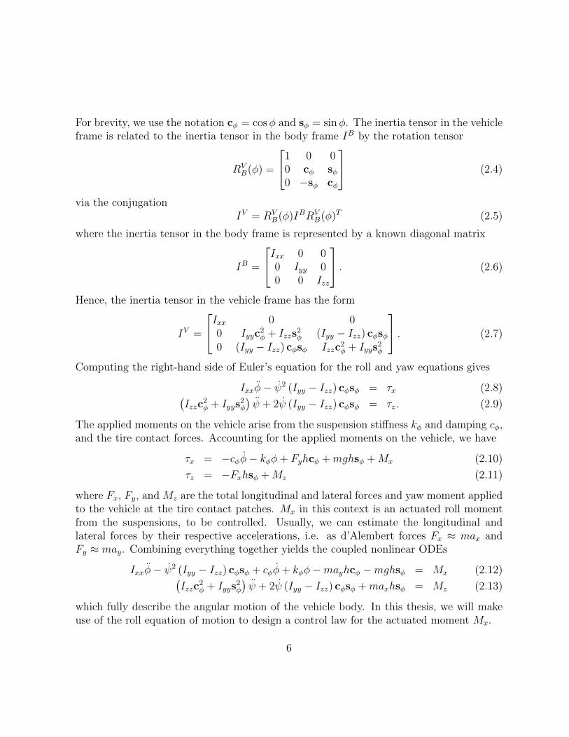
For brevity, we use the notation cφ = cosφ and sφ = sinφ. The inertia tensor in the vehicleframe is related to the inertia tensor in the body frame IB by the rotation tensor
RVB(φ) =
1 0 00 cφ sφ0 −sφ cφ
(2.4)
via the conjugationIV = RV
B(φ)IBRVB(φ)T (2.5)
where the inertia tensor in the body frame is represented by a known diagonal matrix
IB =
Ixx 0 00 Iyy 00 0 Izz
. (2.6)
Hence, the inertia tensor in the vehicle frame has the form
IV =
Ixx 0 00 Iyyc
2φ + Izzs
2φ (Iyy − Izz) cφsφ
0 (Iyy − Izz) cφsφ Izzc2φ + Iyys
2φ
. (2.7)
Computing the right-hand side of Euler’s equation for the roll and yaw equations gives
Ixxφ− ψ2 (Iyy − Izz) cφsφ = τx (2.8)(Izzc
2φ + Iyys
2φ
)ψ + 2ψ (Iyy − Izz) cφsφ = τz. (2.9)
The applied moments on the vehicle arise from the suspension stiffness kφ and damping cφ,and the tire contact forces. Accounting for the applied moments on the vehicle, we have
τx = −cφφ− kφφ+ Fyhcφ +mghsφ +Mx (2.10)
τz = −Fxhsφ +Mz (2.11)
where Fx, Fy, and Mz are the total longitudinal and lateral forces and yaw moment appliedto the vehicle at the tire contact patches. Mx in this context is an actuated roll momentfrom the suspensions, to be controlled. Usually, we can estimate the longitudinal andlateral forces by their respective accelerations, i.e. as d’Alembert forces Fx ≈ max andFy ≈ may. Combining everything together yields the coupled nonlinear ODEs
Ixxφ− ψ2 (Iyy − Izz) cφsφ + cφφ+ kφφ−mayhcφ −mghsφ = Mx (2.12)(Izzc
2φ + Iyys
2φ
)ψ + 2ψ (Iyy − Izz) cφsφ +maxhsφ = Mz (2.13)
which fully describe the angular motion of the vehicle body. In this thesis, we will makeuse of the roll equation of motion to design a control law for the actuated moment Mx.
6
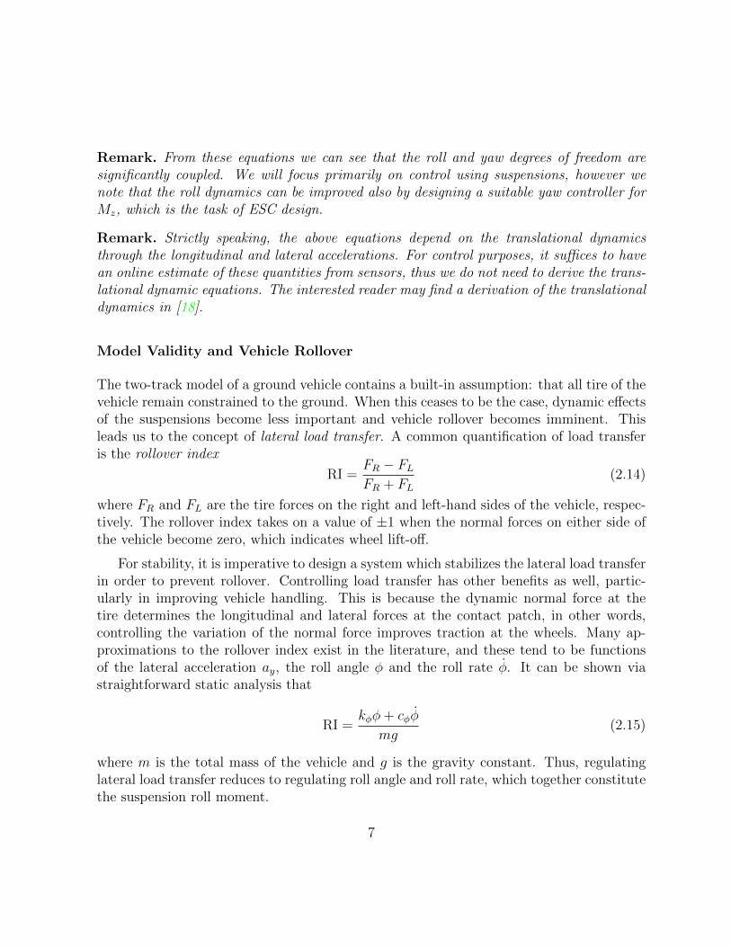
Remark. From these equations we can see that the roll and yaw degrees of freedom aresignificantly coupled. We will focus primarily on control using suspensions, however wenote that the roll dynamics can be improved also by designing a suitable yaw controller forMz, which is the task of ESC design.
Remark. Strictly speaking, the above equations depend on the translational dynamicsthrough the longitudinal and lateral accelerations. For control purposes, it suffices to havean online estimate of these quantities from sensors, thus we do not need to derive the trans-lational dynamic equations. The interested reader may find a derivation of the translationaldynamics in [18].
Model Validity and Vehicle Rollover
The two-track model of a ground vehicle contains a built-in assumption: that all tire of thevehicle remain constrained to the ground. When this ceases to be the case, dynamic effectsof the suspensions become less important and vehicle rollover becomes imminent. Thisleads us to the concept of lateral load transfer. A common quantification of load transferis the rollover index
RI =FR − FLFR + FL
(2.14)
where FR and FL are the tire forces on the right and left-hand sides of the vehicle, respec-tively. The rollover index takes on a value of ±1 when the normal forces on either side ofthe vehicle become zero, which indicates wheel lift-off.
For stability, it is imperative to design a system which stabilizes the lateral load transferin order to prevent rollover. Controlling load transfer has other benefits as well, partic-ularly in improving vehicle handling. This is because the dynamic normal force at thetire determines the longitudinal and lateral forces at the contact patch, in other words,controlling the variation of the normal force improves traction at the wheels. Many ap-proximations to the rollover index exist in the literature, and these tend to be functionsof the lateral acceleration ay, the roll angle φ and the roll rate φ. It can be shown viastraightforward static analysis that
RI =kφφ+ cφφ
mg(2.15)
where m is the total mass of the vehicle and g is the gravity constant. Thus, regulatinglateral load transfer reduces to regulating roll angle and roll rate, which together constitutethe suspension roll moment.
7
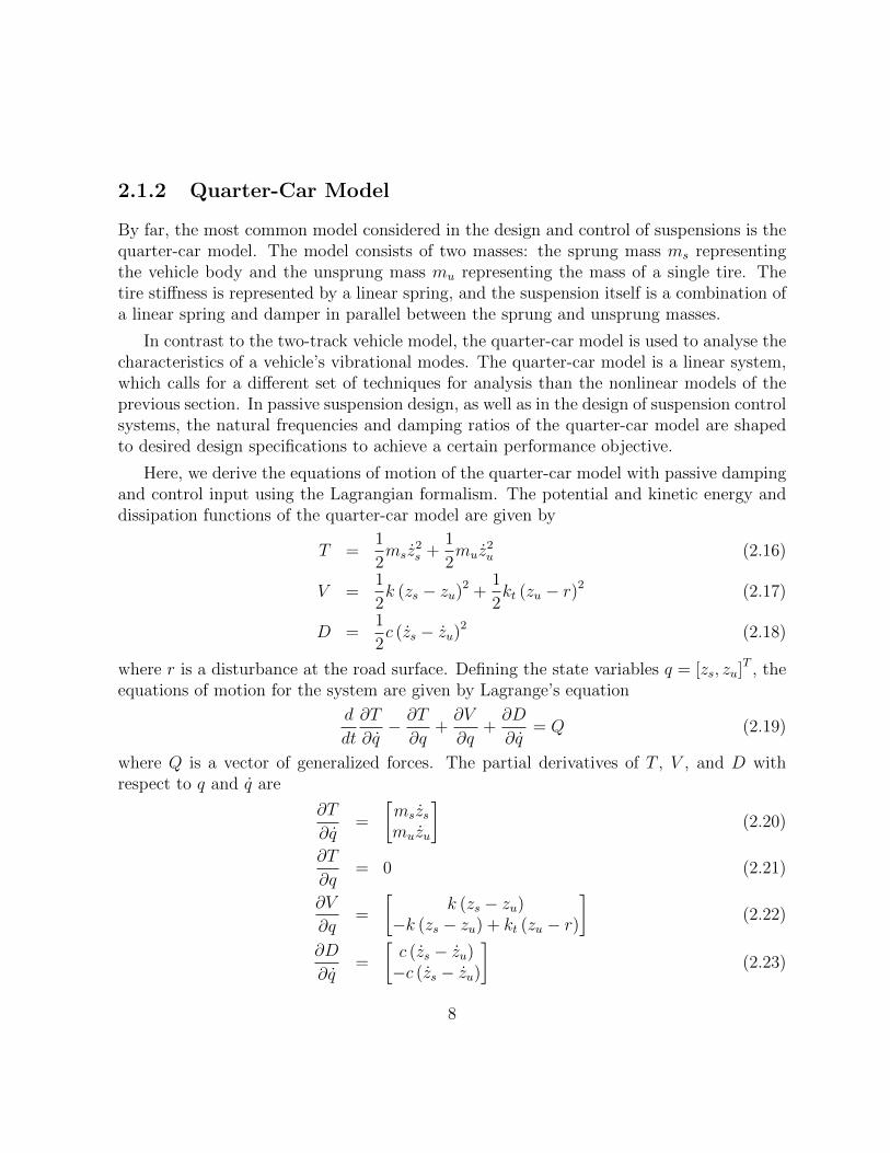
2.1.2 Quarter-Car Model
By far, the most common model considered in the design and control of suspensions is thequarter-car model. The model consists of two masses: the sprung mass ms representingthe vehicle body and the unsprung mass mu representing the mass of a single tire. Thetire stiffness is represented by a linear spring, and the suspension itself is a combination ofa linear spring and damper in parallel between the sprung and unsprung masses.
In contrast to the two-track vehicle model, the quarter-car model is used to analyse thecharacteristics of a vehicle’s vibrational modes. The quarter-car model is a linear system,which calls for a different set of techniques for analysis than the nonlinear models of theprevious section. In passive suspension design, as well as in the design of suspension controlsystems, the natural frequencies and damping ratios of the quarter-car model are shapedto desired design specifications to achieve a certain performance objective.
Here, we derive the equations of motion of the quarter-car model with passive dampingand control input using the Lagrangian formalism. The potential and kinetic energy anddissipation functions of the quarter-car model are given by
T =1
2msz
2s +
1
2muz
2u (2.16)
V =1
2k (zs − zu)2 +
1
2kt (zu − r)2 (2.17)
D =1
2c (zs − zu)2 (2.18)
where r is a disturbance at the road surface. Defining the state variables q = [zs, zu]T , the
equations of motion for the system are given by Lagrange’s equation
d
dt
∂T
∂q− ∂T
∂q+∂V
∂q+∂D
∂q= Q (2.19)
where Q is a vector of generalized forces. The partial derivatives of T , V , and D withrespect to q and q are
∂T
∂q=
[mszsmuzu
](2.20)
∂T
∂q= 0 (2.21)
∂V
∂q=
[k (zs − zu)
−k (zs − zu) + kt (zu − r)
](2.22)
∂D
∂q=
[c (zs − zu)−c (zs − zu)
](2.23)
8
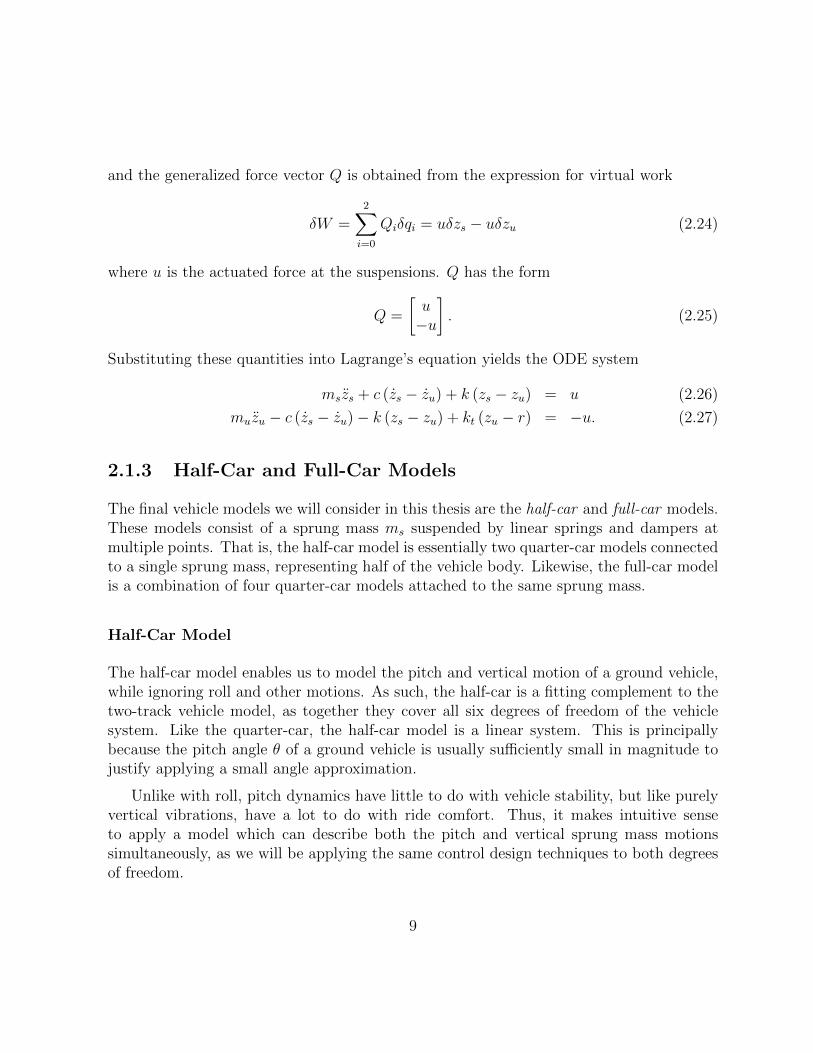
and the generalized force vector Q is obtained from the expression for virtual work
δW =2∑i=0
Qiδqi = uδzs − uδzu (2.24)
where u is the actuated force at the suspensions. Q has the form
Q =
[u−u
]. (2.25)
Substituting these quantities into Lagrange’s equation yields the ODE system
mszs + c (zs − zu) + k (zs − zu) = u (2.26)
muzu − c (zs − zu)− k (zs − zu) + kt (zu − r) = −u. (2.27)
2.1.3 Half-Car and Full-Car Models
The final vehicle models we will consider in this thesis are the half-car and full-car models.These models consist of a sprung mass ms suspended by linear springs and dampers atmultiple points. That is, the half-car model is essentially two quarter-car models connectedto a single sprung mass, representing half of the vehicle body. Likewise, the full-car modelis a combination of four quarter-car models attached to the same sprung mass.
Half-Car Model
The half-car model enables us to model the pitch and vertical motion of a ground vehicle,while ignoring roll and other motions. As such, the half-car is a fitting complement to thetwo-track vehicle model, as together they cover all six degrees of freedom of the vehiclesystem. Like the quarter-car, the half-car model is a linear system. This is principallybecause the pitch angle θ of a ground vehicle is usually sufficiently small in magnitude tojustify applying a small angle approximation.
Unlike with roll, pitch dynamics have little to do with vehicle stability, but like purelyvertical vibrations, have a lot to do with ride comfort. Thus, it makes intuitive senseto apply a model which can describe both the pitch and vertical sprung mass motionssimultaneously, as we will be applying the same control design techniques to both degreesof freedom.
9
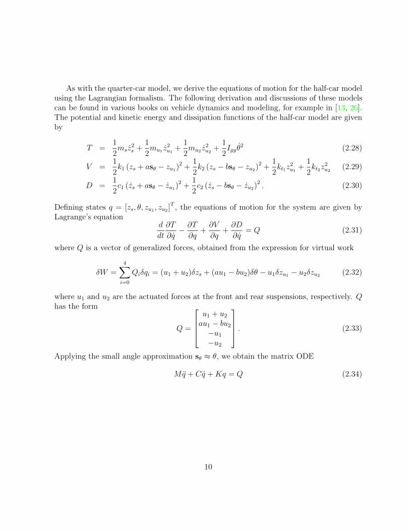
As with the quarter-car model, we derive the equations of motion for the half-car modelusing the Lagrangian formalism. The following derivation and discussions of these modelscan be found in various books on vehicle dynamics and modeling, for example in [13, 26].The potential and kinetic energy and dissipation functions of the half-car model are givenby
T =1
2msz
2s +
1
2mu1 z
2u1
+1
2mu2 z
2u2
+1
2Iyyθ
2 (2.28)
V =1
2k1 (zs + asθ − zu1)
2 +1
2k2 (zs − bsθ − zu2)
2 +1
2kt1z
2u1
+1
2kt2z
2u2
(2.29)
D =1
2c1 (zs + asθ − zu1)
2 +1
2c2 (zs − bsθ − zu2)
2 . (2.30)
Defining states q = [zs, θ, zu1 , zu2 ]T , the equations of motion for the system are given by
Lagrange’s equationd
dt
∂T
∂q− ∂T
∂q+∂V
∂q+∂D
∂q= Q (2.31)
where Q is a vector of generalized forces, obtained from the expression for virtual work
δW =4∑i=0
Qiδqi = (u1 + u2)δzs + (au1 − bu2)δθ − u1δzu1 − u2δzu2 (2.32)
where u1 and u2 are the actuated forces at the front and rear suspensions, respectively. Qhas the form
Q =
u1 + u2
au1 − bu2
−u1
−u2
. (2.33)
Applying the small angle approximation sθ ≈ θ, we obtain the matrix ODE
Mq + Cq +Kq = Q (2.34)
10
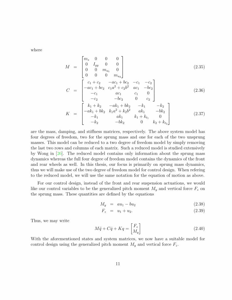
where
M =
ms 0 0 00 Iyy 0 00 0 mu1 00 0 0 mu2
(2.35)
C =
c1 + c2 −ac1 + bc2 −c1 −c2
−ac1 + bc2 c1a2 + c2b
2 ac1 −bc2
−c1 ac1 c1 0−c2 −bc2 0 c2
(2.36)
K =
k1 + k2 −ak1 + bk2 −k1 −k2
−ak1 + bk2 k1a2 + k2b
2 ak1 −bk2
−k1 ak1 k1 + kt1 0−k2 −bk2 0 k2 + kt2
(2.37)
are the mass, damping, and stiffness matrices, respectively. The above system model hasfour degrees of freedom, two for the sprung mass and one for each of the two unsprungmasses. This model can be reduced to a two degree of freedom model by simply removingthe last two rows and columns of each matrix. Such a reduced model is studied extensivelyby Wong in [26]. The reduced model contains only information about the sprung massdynamics whereas the full four degree of freedom model contains the dynamics of the frontand rear wheels as well. In this thesis, our focus is primarily on sprung mass dynamics,thus we will make use of the two degree of freedom model for control design. When referingto the reduced model, we will use the same notation for the equation of motion as above.
For our control design, instead of the front and rear suspension actuations, we wouldlike our control variables to be the generalized pitch moment My and vertical force Fz onthe sprung mass. These quantities are defined by the equations
My = au1 − bu2 (2.38)
Fz = u1 + u2. (2.39)
Thus, we may write
Mq + Cq +Kq =
[FzMy
](2.40)
With the aforementioned states and system matrices, we now have a suitable model forcontrol design using the generalized pitch moment My and vertical force Fz.
11

Full-Car Model
The full-car model is a natural extension of the quarter-car and half-car models to includevertical motion, pitch, and roll of the sprung mass. Each quarter-car represents one of thefour vehicle suspensions. The model is linear, due to imposing a small angle approximationon the roll degree of freedom as well as the pitch degree of freedom. As such, the full-car model is less accurate in modeling the roll motion as roll angle increases. Moreover,since the nonlinear coupling between the yaw rate and lateral acceleration is ignored inthe equations of motion, the full-car model does not give a complete description of thephenomena influencing the roll dynamics. For these reasons, we will not use the full-car model for control design, however we have mentioned it here for completeness. Theinterested reader can find the full derivation of the equations of motion in [13].
2.2 Suspension Control
2.2.1 Active Systems
Active suspension systems have been and remain an area of active research in the auto-motive and control community for over two decades, though they have to date not beenwidely commercialized. These systems are characterized by their ability to both inject anddissipate power in the suspensions. This makes designing a controller using the popularoptimal control methods, e.g. LQR, LQG, H∞, etc. comparatively simple, as the actuatorsare not constrained to only dissipate power, as in semi-active systems.
The most famous example of an actual active suspension system is that in develop-ment by Bose Corporation since 1980 [6, 15]. The Bose suspension system uses linearelectromagnetic actuators at each corner in place of passive dampers and torsion bars tosuspend the vehicle. Moreover, each actuator can be independently controlled in order tooptimize handling and ride. Despite its long development period, the Bose suspension isnot yet present in production vehicles, likely due to prohibitively high costs and powerrequirements. Other active systems include the Active Body Control (ABC) system byMercedes-Benz [1] and the Dynamic Drive System by BMW [22]. In constrast to the Bosesystem, both ABC and Dynamic Drive consist of hydraulic rather then electromagneticactuators. The Dynamic Drive system in particular is actually an active stabilizer barsystem rather than a set of independent actuators. As such, the mechanism is designed tooptimize roll angle.
12
2.2.2 Semi-active Systems
Semi-active suspension systems are characterized by their ability to only dissipate powerin the suspensions. As such, semi-active suspensions must obey a so-called passivity con-straint, which is that semi-active actuators can only exert force opposite their direction ofmotion.
The canonical example of a semi-active actuator is a magnetorheological (MR) damper.MR dampers, also known as variable dampers, contain a rheological fluid whose stiffnessis proportional to the strength of the magnetic field through its volume. MR dampersfunction by inputing a specified electrical current, which by virtue of flowing through asolenoid coil, manipulate the magnetic field within the damper, causing the fluid withinto change its viscous damping properties accordingly. When the magnetic field strength ishigh, the iron particles suspended in the fluid align along the magnetic field lines, whichcauses the fluid to become more viscous and semi-solid. When the magnetic field strengthis low, the fluid returns to a state of lower viscosity. Advantages of semi-active controlusing MR dampers include low power requirements, relatively cheap implementation, andhigh actuator bandwidth. A popular semi-active control system using MR dampers is theMagneRide system by BWI Group, available on many commercial vehicles.
Control of semi-active suspension systems can be viewed as either varying actuator forcegiven certain upper and lower limits, or varying the damping properties of the system. Inthis work, we formulate control laws in terms of actuator forces. Below, we survey somecommon implementations of semi-active control. All of the following control strategiesoriginate from analysis and design on a quarter-car model. An extensive survey of semi-active control methodologies is given by Poussot-Vassal, et al. in [17].
Skyhook Control
Skyhook control is a control strategy specifically designed to dampen motion of the sprungmass, i.e. to improve ride comfort. The derivation of the skyhook control involves findinga control law which emulates a fictitious linear damper with coefficient Csky connected tothe sprung mass and a reference point usually depicted as in the sky, hence the name. Theskyhook control law is given by
Fsky(zs, z) =
−Cskyzs if zsz > 0
0 if zsz < 0(2.41)
where zs is the vertical velocity of the sprung mass and z is the velocity of the suspension,defined by z = zs − zu.
13

Groundhook Control
Groundhook control is a control strategy specifically designed to dampen motion of thewheel, i.e. the unsprung mass. The goal of groundhook control is to lessen variation in thedynamic tire force, which improves the handling properties of the vehicle. The derivation ofthe groundhook control, similar to skyhook, involves finding a control law which emulatesa fictitious linear damper with coefficient Cgnd connected to the unsprung mass and areference point on the ground. The groundhook control law is given by
Fgnd(zs, z) =
−Cgndzu if zuz < 0
0 if zuz > 0(2.42)
where zu is the vertical velocity of the unsprung mass and z is the velocity of the suspension.
Hybrid Control
The hybrid control strategy, as the name suggests, blends the skyhook and groundhooklaws to produce a controller which improves both ride comfort and handling. The hybridcontrol law is defined by
Fhyb = αFsky + (1− α)Fgnd (2.43)
where α ∈ [0, 1] is a constant. Clearly, a value of α = 1 signifies pure skyhook control,and a value of α = 0 signifies pure groundhook control. Various design criteria existfor choosing an intermediate α which blends the skyhook and groundhook effects. Theblending parameter α can also be designed to vary situationally for adaptive control. Inparticular, an adaptive algorithm for hybrid control of semi-active suspensions is given byAgrawal and Khajepour in [2, 3], which will provide some inspiration for the sections onadaptivity.
Clipped Optimal Control
Another method of semi-active control, slightly different from the three methods above,is to design a control law assuming an active actuator using optimal control methods and”clipping” it by imposing the passivity constraint. The control law Fa for the active systemcan be computed using well-known techniques such as LQR, LQG, or H∞, among others,and applying the passivity constraint, one obtains
Fsa =
Fa if zsz > 0
0 if zsz < 0(2.44)
14
2.3 Optimization and Control Allocation
2.3.1 Control Allocation
Now that we have introduced the vehicle models of interest and the common methods ofsuspension control, we will turn our attention to the subject of control allocation. Controlallocation is a relatively new area of control systems research which has emerged over thecourse of the last couple decades, which has been and continues to find new applications innumerous areas of research ranging from automotive systems, aerospace, marine systems,and robotics. Control allocation techniques have high utility when designing systems whichare overactuated, hence their applications in flight controls and growing prominence in theautomotive sector.
The general structure of a control system designed with the control allocation method-ology is divided into two distinct parts: the high-level controller and the control allocator.The control signals generated by the high-level controller are referred to as the virtual con-trol signals, so-called because these control signals need not correspond to any one physicalactuator. In the context of vehicle dynamics controllers, in either automotive or aerospacedomains, the virtual signals correspond to generalized forces and moments applied to thevehicle CG. The control allocator, as the name suggests, is to distribute the control actionsproduced by the high-level controllers among the available actuators physically present inthe system.
The control allocation module is typically defined as an optimization problem, in whichcase we may refer to the process as optimal control allocation. The central objective of theallocation task is to minimize the control allocation error, which is the difference betweenthe virtual control signal and the combined effort of the actuators. If we denote by v ∈ Vthe virtual controls, and by u ∈ U the actuator efforts, then typically we can find a mappingh : U → V called an effector model which relates the actuator efforts to the virtual controls.In general, this mapping can be static, time-varying, state-dependent, linear or nonlinear.The control allocation error is then defined as the quantity v − h(u). In the case that theeffector model is a linear mapping, it is often referred to as the control effectiveness matrixof the system, and denoted by B.
Depending on the preferences of the designer, the defining optimization problem of thecontrol allocation can be either linear, quadratic, generally convex, or generally nonlinearin form. In part, this is determined by the chosen effector model h, but also by the overallstructure of the objective function, and of the constraints defining the feasible actuationsU . In this work, we restrict ourselves to the case of a linear effector model, a quadratic
15

objective function, and linear constraints. This formulation is sometimes referred to asconstrained quadratic control allocation, but in general can be thought of as a quadraticprogramming problem with linear constraints.
The primary objective of the control allocation, as stated before, is to minimize thecontrol allocation error. Given the set of feasible control actions U ⊂ Rn, the quadraticcontrol allocation problem has the following formulation:
minu∈U
γ
2‖v −Bu‖2
Wv+
1
2‖u− u0‖2
Wu(2.45)
where v are the virtual control signals, u are the actuator signals, u0 ∈ Rn is a givenvector, γ ∈ R, Wv,Wu > 0 are positive definite weighting matrices and ‖x‖W = (xTWx)1/2
denotes the L2-norm weighted by W . On account of the use of the L2-norm, this setup issometimes referred to as L2-optimal control allocation. With this form of objective function,the optimal solution is a compromise between minimizing the control allocation error, andthe deviation of the actuations from some specified equilibrium point u0. The relativeimportance of either objective is controllable by designing the weighting matrices Wv,Wu
and the parameter γ appropriately. It can be shown that as the parameter γ → ∞, thesolution of the QP problem (2.45) approaches the solution of the sequential least-squares(SLS) formulation
minu∈Ω
‖u− u0‖Wu
s. t. Ω = arg minu∈U
‖v −Bu‖Wv
(2.46)
which minimizes the control allocation error with first priority, followed by the deviationfrom equilibrium. Thus, the quadratic control allocation can functionally solve for thesame optimal control distribution as the more explicit SLS formulation, while at the sametime enabling efficient computation using contemporary numerical methods designed forsolving quadratic programs.
Advantages of the control allocation approach to control system design include straight-forward implementation of actuator constraints, adaptivity and fault tolerance. The useof an optimization process to minimize the control allocation error ensures that the ac-tuator efforts match the virtual control as well as possible. Secondary objectives can beeasily incorporated into the control strategy by modifying various aspects of the objectivefunction. We will revisit these ideas later in the sections on control allocator design.
The research herein can be viewed as a continuation of that presented by Schofieldand Hagglund in [18, 19, 20, 21] where control allocation via quadratic programming wasused for simultaneous yaw stabilization and rollover detection and prevention using an
16
active braking system. Schofield’s research is an application of the more general theory ofconstrained quadratic control allocation explored by Harkegard in [11], where applicationof the subject to flight controls was also covered. In [10], Harkegard formulated an active-set method for solution of the quadratic control allocation problem. Harkegard generalizedthe quadratic control allocation paradigm to include compensation for actuator dynamicsin [12].
Other applications of control allocation techniques in vehicle dynamics research includethe study by Wang and Wang [25] where quadratic control allocation was used with torquevectoring for fault tolerant stability control of a 4WD electric vehicle. Nonlinear program-ming methods in control allocation have been used as well for the design of ESC systems,for example by Tøndel, Tjønnas, and Johansen in [23, 24]. .
Control allocation as a subject is diverse and covers many other formulations than thequadratic case applied in this work. Moreover, the subject is continually finding new appli-cations. Those interested in a survey of control allocation methods and their applicationsmay see [14].
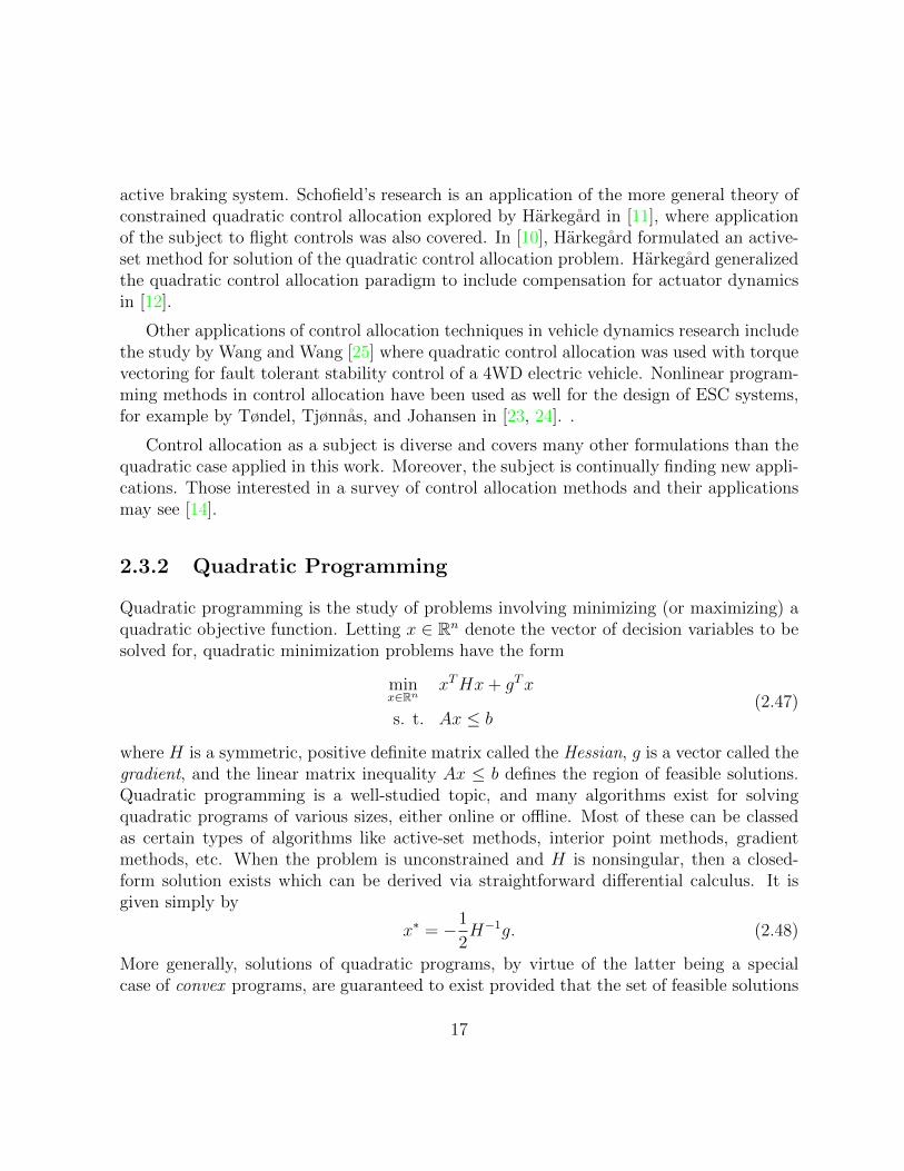
2.3.2 Quadratic Programming
Quadratic programming is the study of problems involving minimizing (or maximizing) aquadratic objective function. Letting x ∈ Rn denote the vector of decision variables to besolved for, quadratic minimization problems have the form
minx∈Rn
xTHx+ gTx
s. t. Ax ≤ b(2.47)
where H is a symmetric, positive definite matrix called the Hessian, g is a vector called thegradient, and the linear matrix inequality Ax ≤ b defines the region of feasible solutions.Quadratic programming is a well-studied topic, and many algorithms exist for solvingquadratic programs of various sizes, either online or offline. Most of these can be classedas certain types of algorithms like active-set methods, interior point methods, gradientmethods, etc. When the problem is unconstrained and H is nonsingular, then a closed-form solution exists which can be derived via straightforward differential calculus. It isgiven simply by
x∗ = −1
2H−1g. (2.48)
More generally, solutions of quadratic programs, by virtue of the latter being a specialcase of convex programs, are guaranteed to exist provided that the set of feasible solutions
17

defined by the constaints is itself a convex set. For constrained problems, however, closed-form expressions of these solutions are not guaranteed to exist, hence the need for analgorithmic solver.
For online computation, as required for constrained quadratic control allocation, active-set methods are preferable because they are relatively fast and have the property that eachiteration of the algorithm produces a feasible suboptimal solution. A couple contemporarysolvers that use active-set methods and which have been previously employed in onlineoptimization are qpOASES1 developed by Ferreau in [7] and QCAT2 (Quadratic Control Al-location Toolbox) by Harkegard in [9, 10].
The basic idea behind active-set methods is that at each iteration, a subset of theinequality constraints are taken to be equality constraints and the rest are ignored. Theset of constraints W which are ”active” is termed the working set. The optimization isthen performed on this set to find the optimal perturbation p from the current suboptimalsolution ui. This generates a new suboptimal solution ui+1 = ui + p. If ui+1 is feasible,then the solution is checked for optimality by looking at the Lagrange multipliers. If thesolution is found to be optimal, then the algorithm terminates, else the working set W isupdated with new active constraints and the algorithm begins a new iteration.
For the experiments documented in this work, the QCAT toolbox was used for onlineoptimization on a dSPACE AutoBox. The algorithm, as formulated by Harkegard in [10]is reproduced here for reference. Harkegard noted that the quadratic objective function in(2.45) may be rewritten as
γ
2‖v −Bu‖2
Wv+
1
2‖u− u0‖2
Wu=
1
2
∥∥∥∥∥(
(γWv)12 B
W12u
)u−
((γWv)
12 v
W12u u0
)∥∥∥∥∥2
︸ ︷︷ ︸=:‖Au−b‖2
. (2.49)
Supposing that the set of feasible solutions U is described by box constraints, i.e. we haveui ≤ ui ≤ ui, then the quadratic program reduces to solving
minu∈Rn
‖Au− b‖
s. t.
(I−I
)︸ ︷︷ ︸
=:C
u ≤(u−u
)(2.50)
1http://set.kuleuven.be/optec/Software/qpOASES-OPTEC2http://research.harkegard.se/qcat/index.html
18
which can be solved efficiently using Algorithm 1 below.
Those interested in the theory and application of convex optimization (including quadraticprogramming) may see the text [5] by Boyd and Verdenberghe, which is freely availableonline from the authors3.
3http://www.stanford.edu/ boyd/cvxbook/
19

Input: A feasible initial iterate u0.Output: The optimal control distribution u∗.for i = 0, 1, 2, ... do
Given the suboptimal iterate ui and the working set of active constraints W ,solve the following equality constrained problem for the optimal perturbation p:
minp∈Rn
∥∥A(ui + p)− b∥∥
s. t.Bp = 0pj = 0, ∀j ∈ W
(2.51)
if ui + p is feasible thenSet ui+1 = ui + p;Compute the Lagrange multipliers λ, µ via
AT(Aui+1 − b
)=(BT CT
i
)(µλ
)(2.52)
where Ci is the matrix formed by the rows of C corresponding to constraintsin the working set W for the current iteration;if λ ≥ 0 then
The optimal solution has been found;return u∗ = ui+1;
elseRemove the constraint corresponding to the most negative Lagrangemultiplier λ from the working set W ;
end
end
endAlgorithm 1: QCAT active-set algorithm.
20

Chapter 3
Design and Simulation
3.1 High-Level Controller Design
In the following two chapters, we present the design, simulation, implementation, andexperimentation of the coordinated suspension control system, or CSC. We begin by de-veloping the high-level controllers for the roll, pitch and vertical motions of the vehicle.As explained in the previous chapter, our approach to coordinated suspension control usesthese high-level controllers to generate the virtual control signals, e.g. the roll and pitchmoments Mx and My and the vertical CG force Fz, which the actuators must work to-gether to exert on the vehicle body. For this, we apply techniques from both nonlinear andadvanced linear control theory, namely sliding mode control (SMC).
Sliding mode control is a nonlinear control technique which guarantees asymptoticstability of the closed loop system even in the presence of modeling errors. This is particularuseful, since the vehicle dynamics are nonlinear in nature and parametric uncertainties canhave a large impact on the system behavior. The use of sliding mode control thus enablesus to take these nonlinear behaviors into account, which is particularly important at highspeeds and in harsh maneuvers. For general background on nonlinear control theory andsliding mode control in particular, the interested reader may see [16].
3.1.1 Roll Control
The roll dynamics of the ground vehicle may be represented by the two-track model. Recallthat the nonlinear angular dynamic equation of motion for the roll degree of freedom is
21
given by
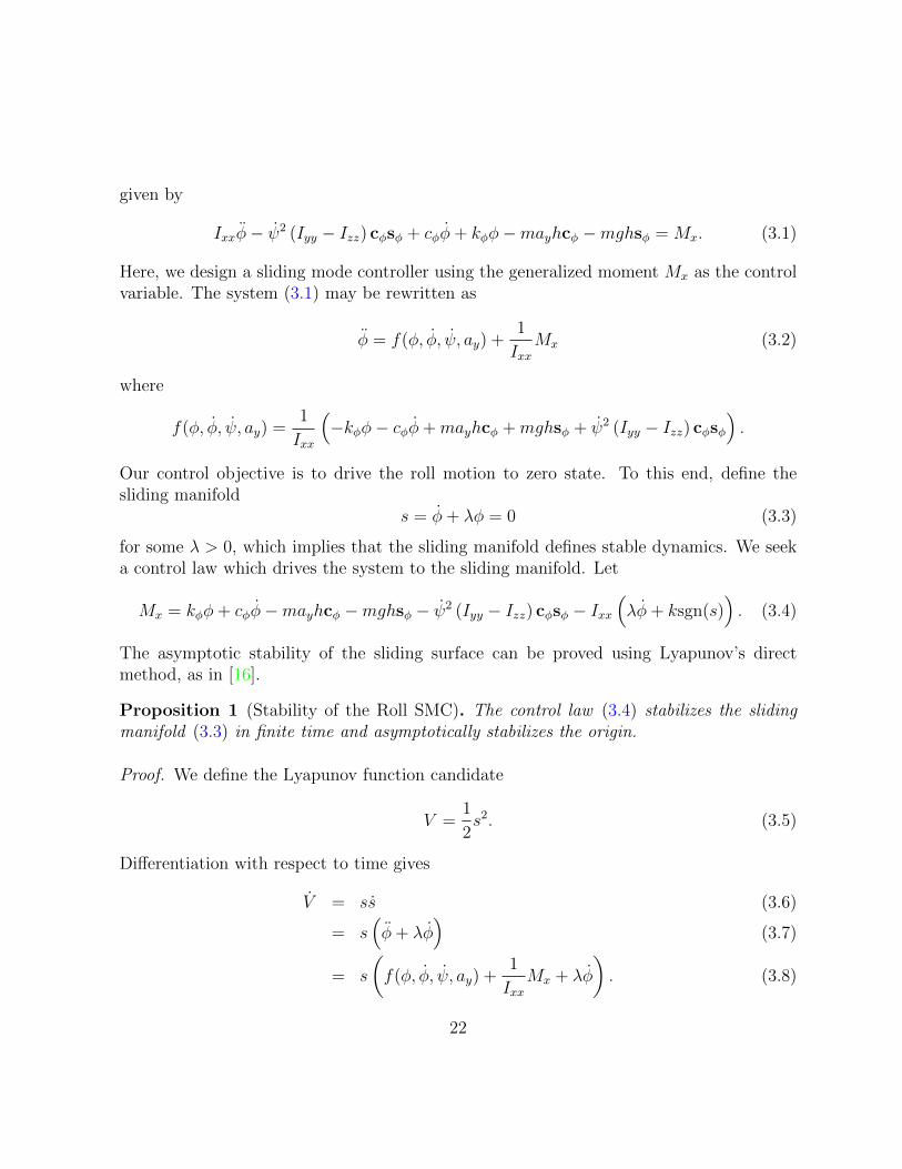
Ixxφ− ψ2 (Iyy − Izz) cφsφ + cφφ+ kφφ−mayhcφ −mghsφ = Mx. (3.1)
Here, we design a sliding mode controller using the generalized moment Mx as the controlvariable. The system (3.1) may be rewritten as
φ = f(φ, φ, ψ, ay) +1
IxxMx (3.2)
where
f(φ, φ, ψ, ay) =1
Ixx
(−kφφ− cφφ+mayhcφ +mghsφ + ψ2 (Iyy − Izz) cφsφ
).
Our control objective is to drive the roll motion to zero state. To this end, define thesliding manifold
s = φ+ λφ = 0 (3.3)
for some λ > 0, which implies that the sliding manifold defines stable dynamics. We seeka control law which drives the system to the sliding manifold. Let
Mx = kφφ+ cφφ−mayhcφ −mghsφ − ψ2 (Iyy − Izz) cφsφ − Ixx(λφ+ ksgn(s)
). (3.4)
The asymptotic stability of the sliding surface can be proved using Lyapunov’s directmethod, as in [16].
Proposition 1 (Stability of the Roll SMC). The control law (3.4) stabilizes the slidingmanifold (3.3) in finite time and asymptotically stabilizes the origin.
Proof. We define the Lyapunov function candidate
V =1
2s2. (3.5)
Differentiation with respect to time gives
V = ss (3.6)
= s(φ+ λφ
)(3.7)
= s
(f(φ, φ, ψ, ay) +
1
IxxMx + λφ
). (3.8)
22
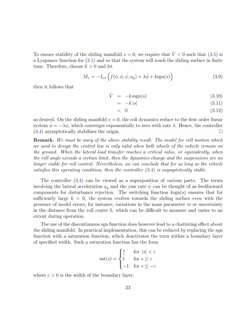
To ensure stability of the sliding manifold s = 0, we require that V < 0 such that (3.5) isa Lyapunov function for (3.1) and so that the system will reach the sliding surface in finitetime. Therefore, choose k > 0 and let
Mx = −Ixx(f(φ, φ, ψ, ay) + λφ+ ksgn(s)
)(3.9)
then it follows that
V = −kssgn(s) (3.10)
= −k |s| (3.11)
< 0 (3.12)
as desired. On the sliding manifold s = 0, the roll dynamics reduce to the first order linearsystem φ = −λφ, which converges exponentially to zero with rate λ. Hence, the controller(3.4) asymptotically stabilizes the origin.
Remark. We must be wary of the above stability result. The model for roll motion whichwe used to design the control law is only valid when both wheels of the vehicle remain onthe ground. When the lateral load transfer reaches a critical value, or equivalently, whenthe roll angle exceeds a certain limit, then the dynamics change and the suspensions are nolonger viable for roll control. Nevertheless, we can conclude that for as long as the vehiclesatisfies this operating condition, then the controller (3.4) is asymptotically stable.
The controller (3.4) can be viewed as a superposition of various parts. The termsinvolving the lateral acceleration ay and the yaw rate ψ can be thought of as feedforwardcomponents for disturbance rejection. The switching function ksgn(s) ensures that forsufficiently large k > 0, the system evolves towards the sliding surface even with thepresence of model errors, for instance, variations in the mass parameter m or uncertaintyin the distance from the roll center h, which can be difficult to measure and varies to anextent during operation.
The use of the discontinuous sgn function does however lead to a chattering effect aboutthe sliding manifold. In practical implementation, this can be reduced by replacing the sgnfunction with a saturation function, which deactivates the term within a boundary layerof specified width. Such a saturation function has the form
sat(s) =
sε
for |s| < ε
1 for s ≥ ε
−1 for s ≤ −ε
where ε > 0 is the width of the boundary layer.
23
3.1.2 Pitch and Vertical Motion Control
As with the roll controller derived above, we design sliding mode controllers for the pitchand vertical degrees of freedom of the vehicle. For this design, we will apply the two degreeof freedom half-car model to represent the dominant dynamics. Recall that the equationof motion of the half-car model is given by the matrix equation (2.40)
Mq + Cq +Kq =
[FzMy
](3.13)
where the system states of interest are q = [zs, θ]T and the control inputs are given by
w = [Fz,My]T . Here, we design sliding mode controllers using these generalized efforts as
the control variables. Rearranging (3.13), we have
q = −M−1 (Kq + Cq − w) . (3.14)
Defining the sliding manifold σ = 0 by the equation
σ = q + Λq = 0 (3.15)
where Λ > 0 is a positive definite matrix. This implies that the spectrum of Λ is containedin the right half-plane, and so the sliding manifold defines stable dynamics. We seek acontrol law which drives the dynamics of the vehicle asymptotically to the sliding manifold.Let [
FzMy
]= Kq + Cq −M−1 (Λq + κsgn(σ)) (3.16)
where sgn(σ) is to be understood as the vector whose ith element is the ordinary signumfunction applied to the corresponding element of σ, and κ > 0 is a positive definite diagonalmatrix.
As with the roll controller, the asymptotic stability of the sliding surface can be provedusing Lyapunov’s direct method, as in [16].
Proposition 2 (Stability of the Pitch and Vertical SMCs). The control law (3.16) stabilizesthe sliding manifold (3.15) in finite time and asymptotically stabilizes the origin.
Proof. We define the Lyapunov function candidate
V =1
2σTσ. (3.17)
24
Differentiation with respect to time gives
V = σT σ (3.18)
= σT (q + Λq) (3.19)
= σT(−M−1 (Kq + Cq − w) + Λq
). (3.20)
To ensure stability of the sliding manifold σ = 0, we require that V < 0 such that (3.17)is a Lyapunov function for (3.13) and so that the system will reach the sliding surface infinite time. Therefore, choose κ = diag[k1, k2] for k1, k2 > 0 and let
w = Kq + Cq −M−1 (Λq + κsgn(σ)) (3.21)
then it follows that
V = −σTκsgn(σ) (3.22)
= −k1 |σ1| − k2 |σ2| (3.23)
< 0 (3.24)
as desired. On the sliding manifold σ = 0, the system dynamics reduce to the first orderlinear system q = −Λq, which converges exponentially to zero. Hence, the controller (3.16)asymptotically stabilizes the origin.
As with the roll controller, for sufficiently large gains k1, k2 > 0, the system evolvestowards the sliding surface even with the presence of model errors, for instance, unmodelednonlinearities, variations in the mass parameterm, or uncertainty in the suspension stiffnessand damping properties. The chattering effect about the sliding manifold can likewise bealleviated with the use of a saturation function in place of the sgn function.
3.2 Control Allocator Design
In this section, we consider the task of distributing the virtual control action v, definedby the high-level controllers of the previous sections, over the available actuators on thevehicle, and given a set of admissible control actions U ⊂ R4 defined by the actuatorconstraints. This is accomplished by solving an L2-optimal control allocation problem byway of quadratic programming with linear constraints, which was briefly introduced in theprevious chapter. The decision variables to be solved for are the actuator control signals,
25
which is to be done at each time step during operation. Specifically, we solve the followingproblem:
minu∈U
γ
2‖v −Bu‖2
Wv+
1
2‖u− u0‖2
Wu(3.25)
where v = [Mx,My, Fz]T are the virtual control signals, u = [u1, u2, u3, u4]T are the actuator
signals, u0 ∈ R4 is a given vector, γ ∈ R, Wv,Wu > 0 are positive definite weightingmatrices and ‖x‖W = (xTWx)1/2 denotes the L2-norm weighted by W .
The purpose of the first term in the objective function (3.25) is to minimize the al-location error, i.e. the difference between the desired control action and the combinedoutput of the actuators. In this context, B : U → V is the control effectiveness matrix, alinear mapping from the space of actuator signals into the space of virtual control signals.Specifically, B relates the lower-level controls to their output in terms of the generalizedCG forces and moments.
The second term is meant to penalize deviation of the actuations from some givenequilibrium state and to ensure convexity of the optimization problem, as in general, mul-tiple solutions might exist such that v = Bu on account of the overactuated nature of thesystem.
In the following sections, we elaborate on the setup of the control allocation problem.We derive the control effectiveness matrix and discuss appropriate actuator constraints forimplementation with active and semi-active suspension systems.
3.2.1 Control Effectiveness Matrix
In this work, we restrict our attention to the vertical force actuations u on the sprung massproduced by four independent suspension actuators, either active or semi-active in nature.Assuming that the suspension forces always actuate perpendicularly to the plane of thesprung mass, the roll and pitch moments and the vertical force on the CG in terms of thesuspension forces are given by
Mx =T
2(u1 − u2 + u3 − u4) (3.26)
My = a (u1 + u2)− b (u3 + u4) (3.27)
Fz = u1 + u2 + u3 + u4 (3.28)
The control effectiveness matrix B is defined as the mapping relating the lower-level actu-ator controls to the virtual control signals v. Under these assumptions, the map is linear
26

and is given by
B =
T2−T
2T2−T
2
a a −b −b1 1 1 1
. (3.29)
Implicitly, this design of the end effector map assumes that the angular motion ofthe sprung mass nor the geometric configuration of the suspensions affects the controlallocation. In reality, the direction that the suspensions push and pull on the sprung masschange as the vehicle rolls and pitches and the suspensions themselves compress and extend.Thus, one might expect that the map B would be a function of the vehicle states. As such,it is reasonable to expect some error in the control allocation due to these approximations.
3.2.2 Active Systems
We now consider the design of the control allocation module for use with independentactive suspensions. In the simplest case, i.e. assuming that the active suspensions areperfect actuators without constraints, then U = R4 and the QP problem (3.25) has ananalytical solution
u =
(BTWvB +
1
γWu
)−1(BTWvv −
1
γWuu0
)(3.30)
which can be derived using straightforward calculus. Furthermore, for active suspensionsystems, u0 is usually taken to be zero, giving
u =
(BTWvB +
1
γWu
)−1
BTWvv. (3.31)
In practical situations we have constraints on the actuator outputs, that is we have boxconstraints ui ≤ ui ≤ ui for each i, possibly time or state-dependent, such that U =∏4
i=1[ui, ui]. The QP problem to be solved is thus
minu∈R4
γ
2‖v −Bu‖2
Wv+
1
2‖u− u0‖2
Wu
s. t. u ≤ u ≤ u(3.32)
Depending on the dynamics of the actuators in question, rate constraints might need tobe defined as well. These can be easily realized by adding more linear constraints to theQP formulation.
27
In the case of constrained optimization, it is necessary to employ an online optimizationalgorithm for solution of the above QP in real time, such as an active-set or interior pointmethod, since analytical solutions do not exist in general for constrained optimizations.
Remark. Alternatively, the closed form solution (3.31) may be used with saturation to en-force the constraints, however optimality of the control allocation is not ensured in this case.Generally speaking, this is not advisable, as the QP problem is small enough dimensionallyto allow for rapid solution and real-time implementation using active-set methods.
3.2.3 Semi-active Systems
Having first considered the simpler case of fully active suspensions, we now turn our atten-tion to the more complicated case of semi-active suspensions. We present an implementa-tion of semi-active suspension control within the framework of optimal control allocation,using the QP constraints.
In the case of semi-active suspensions (MR dampers), we have the same type of QPproblem as in (3.32), however the constaints on the actuators become essentially state-dependent. For semi-active control we require feedback of the suspension states to deter-mine the minimum and maximum actuator outputs. Assuming that we have a static MRdamper model Fd = Fd(z, i) to model the damping force, the minimum and maximumforce output vectors u and u can be easily defined. The internal dynamics of MR dampers,being electromagnetic in nature, can be assumed to operate much faster than the mechan-ical motions of the suspensions. On this assumption, we can ignore rate constraints anddefine the upper and lower bounds on u by
ui = Fd(zi, imin) ∧ Fd(zi, imax) (3.33)
ui = Fd(zi, imin) ∨ Fd(zi, imax) (3.34)
where ∧ and ∨ denote the minimum and maximum elements, respectively, zi is the sus-pension velocity at the ith wheel, imin and imax are minimum and maximum admissiblecurrents to the dampers, respectively. In contrast to the active suspension, it is useful totake u0 = [u1,0, u2,0, u3,0, u4,0]T where
ui,0 = Fd(zi, i0) (3.35)
for some baseline current input i0 ∈ [imin, imax]. For the objective of minimizing the energy
28

consumption of the MR dampers, we take i0 = imin. The QP problem (3.25) thus becomes
minu∈R4
γ
2‖v −Bu‖2
Wv+
1
2‖u− u0‖2
Wu
s. t. u(z) ≤ u ≤ u(z)
u0 = Fd(z, i0)
(3.36)
where z = [z1, z2, z3, z4]T and the objective function and constraints are dynamically up-dated at each time step in accordance with the suspension dynamics. As with the con-strained active system, it is necessary to employ an online optimization algorithm for real-time solution of the QP problem. As state previously, active-set methods are well-suitedto this task.
3.2.4 Adaptivity and Fault Tolerance
In this section, we turn our attention to the idea of making the above control allocationproblem situationally adaptive. It makes intuitive sense that while driving, some situationswould require roll control, such as taking a tight turn or making an evasive maneuver,whereas others would require pitch control, such as during periods of heavy accelerationand breaking. If we assume that the control system is fully active and unconstrained, thensuch an adaptation scheme is unnecessary, since the overactuation of the system ensuresthat both desired roll and pitch moments can always be applied to the vehicle. As soonas actuator constraints are brought into the picture, for example, with semi-active control,this ceases to be the case, and it would be advantageous to design criteria whereby rollcontrol would be prefered and likewise for pitch control.
Additionally, there are situations where decentralized suspension control might be desir-able in comparison to the centralized scheme afforded by the integrated system presentedin the previous sections. For example, consider a vehicle driving straight at constant speedover a bumpy road. The roll and pitch vibrations, though extant, are not as large asthey would be during intense maneuvering, so coordinated roll and pitch control are likelynot necessary. Instead, the suspensions should be concentrating their efforts on the ridecomfort objective, that is, controlling the sprung mass acceleration at each single corner,independently. As we shall see, by defining suitable adaptation parameters, the objectivefunction of the control allocator module can be modified such that single-corner suspensioncontrol and coordinated roll and pitch control can be integrated into a single framework.
Finally, it is important that the control system is able to handle actuator failures. If oneor more of the actuators malfunctions and becomes unusable, then the control allocation
29
problem should be modified to account for this failure and even suggest for the workingactuators to compensate for the failure. All of this is possible within the framework ofoptimal control allocation.
Fault Tolerance
In the real world, things break under stress. If in extreme situations, the suspensionsmalfunction and cannot actuate forces correctly, the control allocation algorithm shouldbe tuned such that the failed actuator is removed from the optimization process. Thisintroduces yet another aspect of adaptivity and robustness in the control system, as theoptimization process allows for the remaining actuators to compensate for system failuresif they are able.
Fault tolerance can be achieved by modifying the control effectiveness matrix B andthe vector u0 in real time. If the ith actuator fails, then set the ith column of the matrix Band the ith element of u0 to zero. This ensures that ui = 0 and removes the failed actuatorfrom consideration in the control allocation problem.
Adaptation Parameters
Here, we seek to define parameters αMx and αMy which quantify the need for roll and pitchcontrol, respectively. For this, we must first analyze qualitatively when coordinated rolland pitch control are justified.
As stated at the beginning of this section, roll control is useful in extreme maneuvering,when cornering and when making evasive maneuvers. For the roll adaptation, we can takeinspiration from rollover detection and prevention systems in the literature, which define athreshold roll angle φ after which the control system activates. Ideally, however, we wouldlike to include some predictive action into the adaptation process. For this, we can useas well the lateral acceleration ay for adaptation. As with the roll angle, we may definea threshold ay such that when the lateral acceleration exceeds this amount, the controlsystem activates roll control for improved cornering.
As in the figure, the inputs to the adaptation scheme are the roll angle φ and the lateralacceleration ay. First, both signals are normalized by their threshold values φ and ay. Theroll threshold is chosen to be roughly half of the so-called critical roll angle φc after whichrollover is imminent. The steering threshold is chosen large enough so as to ignore smallperturbations. The normalized signals are then each passed through the heuristic notchfunction h which maps the signals to values in the closed interval [0, 1]. The two signals
30
are then added together and sent through a saturation block such that their sum remainsbetween 0 and 1. Finally, the summed signal is passed through a smoothing filter whoseoutput is αMx .
As such, the signal αMx remains near zero, the OFF state, when roll motion and steeringaction are minimal, and quickly increases to unity, the ON state, when the driver entersa maneuver. Since the signal is a composite of steering angle and roll angle information,αMx will stay at 1 until the maneuver is complete, after which it will return to the OFFstate.
The design of the pitch adaptation parameter is similar, except that instead of roll angle,we consider the pitch angle θ and instead of the steering angle, we use the longitudinalacceleration ax.
As with αMx , the signal αMy remains in the OFF state when pitch motion and forwardacceleration are minimal, and quickly reaches the ON state when the vehicle starts pitching,such as while accelerating or breaking. Since the signal is a composite of pitch angle andacceleration signals, αMy will stay at 1 until the maneuver is complete, after which it willreturn to the OFF state.
With these parameters in mind, we are ready to incorporate an adaptive process intothe control allocation.
Adaptive Allocation
Recall the QP problem formulation (3.36) for the semi-active system:
minu∈R4
γ
2‖v −Bu‖2
Wv+
1
2‖u− u0‖2
Wu
s. t. u(z) ≤ u ≤ u(z)
u0 = Fd(z, i0)
where γ > 0 is sufficiently large. To make the system adaptive and integrated with localsuspension controllers, we redefine two things: the equilibrium control vector u0 and theweighting matrix Wv.
In the previous section, the vector u0 was chosen to minimize energy expenditure bythe MR dampers by defining its elements by the minimal admissible current. In the case ofintegrating local suspension controllers, we instead define this vector by the control signalsfrom these local controllers. If, for example, we consider the skyhook control law for the
31
quarter car model,
Fsky(zs, z) =
Cskyzs if zsz > 0
0 if zsz < 0(3.37)
where zs denotes the vertical velocity of the sprung mass at the suspension and z is thesuspension velocity, we can take u0 = [u1,eq, u2,eq, u3,eq, u4,eq]
T where
ui,eq = Fsky(zs,i, zi) (3.38)
such that the local skyhook suspension control becomes the equilibrium point of the secondterm of the objective function. It becomes the case, then, that if the first term of theobjective function becomes negligible, then the control system reduces to independentskyhook control at each wheel.
Our intuition is clear: we wish to define the weighing matrix Wv for the virtual controlssuch that it becomes significant in situations where coordinated roll and pitch control isjustified, and negligible otherwise. We define α = [αMx , αMy ]T and Wv to be
Wv(α) =
αMx
αMy
αFz
(3.39)
where αMx and αMy are the adaptation parameters developed in the previous section.Additionally, we have the parameter αFz pertaining to the vertical force at the vehicle CG.Since the local suspension controllers are designed to minimize sprung mass motion, thento have this term active at all times would be redundant. Instead, we can define αFz inthe following way:
αFz = αMx ∨ αMy (3.40)
where ∨ denotes the maximum element. Thus, whenever roll or pitch control is initiated,vertical CG motion is nonetheless included as a secondary objective. This is useful insituations where a singular vertical excitation (f.e. a large bump under one wheel) occursduring a maneuver.
By the definitions of the adaptation parameters and the weighting matrix Wv, we havethat the adaptive QP formulation
minu∈R4
γ
2‖v −Bu‖2
Wv(α) +1
2‖u− u0‖2
Wu
s. t. u(z) ≤ u ≤ u(z)
u0 = Fsky(zs, z)
(3.41)
asserts coordinated control when either the roll or pitch adaptations reach the ON state,and likewise asserts localized suspension control when both are in the OFF state, as desired.
32
3.2.5 System Stability with the Control Allocator
Assuming no actuator saturations, then the optimal solution to the QP problem is givenin closed-form by the equation
u =
(BTWvB +
1
γWu
)−1(BTWvv −
1
γWuu0
)(3.42)
which is a static linear map with inputs v and u0. Stability of the control allocation isattained if and only if we have
det
(BTWvB +
1
γWu
)6= 0 (3.43)
which is to say that the mapping (v, u0) 7→ u above is well-defined. In this case, thestability of the closed-loop system is determined by the stability of the controllers definingv and u0. Since the high-level controllers of the previous section were proven to be globallyasymptotically stable, then the static control allocation preserves this property, particularlywhen the control effectiveness matrix B perfectly models the relationship between thevirtual controls and the actuator signals.
When actuator saturation occurs, then the combined control system loses global asymp-totic stability of the origin, as the system equilibria are perturbed to match the applieddisturbances on the vehicle. For example, when the vehicle sustains a cornering maneu-ver, the lateral acceleration reaches a steady-state value. If the vehicle is equipped witha semi-active system, then the constraints inhibit the actuators from exerting a correctiveroll moment in steady-state, which causes the equilibrium roll angle to be nonzero. Suchdrift phenomena cannot be helped with semi-active actuators, however, the control alloca-tion is nevertheless able to preserve asymptotic stability in cases of high excitation, whensaturation is not encountered.
3.3 Simulation Results
The coordinated control system was simulated on a CarSim model of a Chevrolet Equinox.The vehicle entered a fishhook maneuver at a cruising velocity of 100 kph and given notorque input. The fishhook was chosen since the harshness of the maneuver would bringthe vehicle close to rollover. As the roll motion is dominant in this maneuver, the controllergains were tuned to emphasize the suspension roll moment. To prevent chattering of the
33

control signals, the discontinuous sgn functions were replaced by continuous saturationfunctions in the sliding mode control laws. The semi-active actuators were modeled viathe empirical models in (4.1), which will be introduced in the next chapter.
The primary purpose of the simulation study here was to judge the efficacy of thecoordinated controller in minimizing the peak roll and pitch angles, as well as verticalvibrations versus ordinary passive damping. It was also of interest was ascertaining whetheror not the coordinated control of vehicle roll using suspensions would improve the lateralload transfer, i.e. reduce the peak magnitude of the rollover index
RI =FR − FLFR + FL
(3.44)
where FR and FL are the tire forces on the right and left-hand sides of the vehicle, re-spectively. Peak magnitudes were the prefered metric since in harsh maneuvering witha ground vehicle, the extremes of the dynamics are often what lead to instability, as inrollover.
The optimizer employed in simulation was qpOASES, a solver based on an active setmethod developed for real-time implementation of MPC controllers, but which is also well-suited to online quadratic programming in general [7]. A quantitative comparison betweenthe active, semi-active and passive system simulations is included in Table 4.1.
3.3.1 Active System
The results of the active system simulation can be seen in Figures 3.2, 3.4, 3.8, 3.9, 3.10,and 3.11. The active system greatly improved the angular and vertical responses of thevehicle. The absence of constraints on the actuators enabled the suspensions to drivethe angular and vertical dynamics asymptotically to zero. Moreover, the rollover indexwas effectively controlled by the coodinated suspension system. This indicates that thesuspension controller did not deteriorate the vehicle’s handling.
3.3.2 Semi-active System
The results of the semi-active system simulation can be seen in Figures 3.3, 3.6, 3.8, 3.9,3.10, and 3.11. It was supposed that the minimum and maximum admissible currents tothe dampers were imin = 0 A and imax = 5 A. The semi-active suspension system wasseen to perform comparably to the active system, except in periods of low excitation in
34
0 2 4 6 8 10
−150
−100
−50
0
50
100
150
Steering Input
Time [s]
SW
A [d
eg]
Figure 3.1: Steering input for a fishhook maneuver.
the suspensions. Overall, the optimization-based approach to semi-active control succeedsin attenuating the largest vibrations sustained in the fishhook maneuver. Moreover, likethe active system, the semi-active system stabilizes the lateral load transfer (3.44) of thevehicle, effectively preserving the vehicle’s handling and adding an element of rolloverprevention to the system. As expected, the constraints on the actuators are the limitingfactors in the performance of the semi-active system versus the active system.
3.4 Discussion
Overall, the active and semi-active systems performed as expected in simulation. Theactive system retained the stability properties of the high-level controllers due to the un-constrained nature of the assumed actuators. The drawback of semi-active actuators isobviously the presence of the passivity constraint, which precludes global asymptotic sta-bility of the origin under perturbations of sufficient magnitude. Nevertheless, the controlallocation-based approach to semi-active control results in a performance improvementversus passive systems.
Sliding mode controllers were chosen as the preferred high-level controllers in this work,however, there is no particular reason why this should be the case absolutely. Other types
35
0 2 4 6 8 10−1.5
−1
−0.5
0
0.5
1
1.5x 10
4 Virtual Control Signals − Active Suspension
Time [s]
Con
trol
Act
ion
M
x
My
Fz
Figure 3.2: Virtual control signals from the active system simulation.
0 2 4 6 8 10−2.5
−2
−1.5
−1
−0.5
0
0.5
1
1.5
2
2.5x 10
4 Virtual Control Signals − Semi−active Suspension
Time [s]
Con
trol
Act
ion
M
x
My
Fz
Figure 3.3: Virtual control signals from the semi-active system simulation.
36
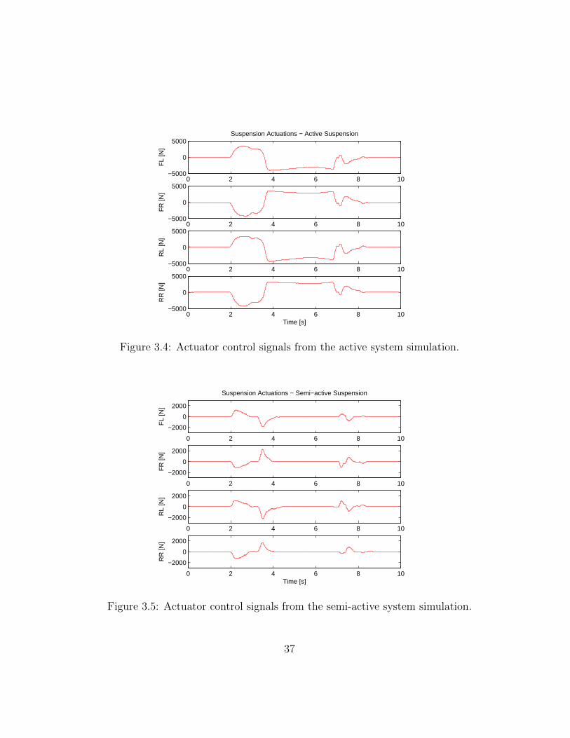
0 2 4 6 8 10−5000
0
5000Suspension Actuations − Active Suspension
FL
[N]
0 2 4 6 8 10−5000
0
5000
FR
[N]
0 2 4 6 8 10−5000
0
5000
RL
[N]
0 2 4 6 8 10−5000
0
5000
Time [s]
RR
[N]
Figure 3.4: Actuator control signals from the active system simulation.
0 2 4 6 8 10
−2000
0
2000
Suspension Actuations − Semi−active Suspension
FL
[N]
0 2 4 6 8 10
−2000
0
2000
FR
[N]
0 2 4 6 8 10
−2000
0
2000
RL
[N]
0 2 4 6 8 10
−2000
0
2000
Time [s]
RR
[N]
Figure 3.5: Actuator control signals from the semi-active system simulation.
37

0 2 4 6 8 100
5Damper Currents − Semi−active Suspension
FL
[A]
0 2 4 6 8 100
5
FR
[A]
0 2 4 6 8 100
5
RL
[A]
0 2 4 6 8 100
5
Time [s]
RR
[A]
Figure 3.6: Current input signals from the semi-active system simulation.
0 2 4 6 8 10−0.5
0
0.5Suspension Velocities − Semi−active Suspension
FL
[m/s
]
0 2 4 6 8 10−0.5
0
0.5
FR
[m/s
]
0 2 4 6 8 10−0.5
0
0.5
RL
[m/s
]
0 2 4 6 8 10−0.5
0
0.5
Time [s]
RR
[m/s
]
Figure 3.7: Suspension velocities from the semi-active system simulation.
38
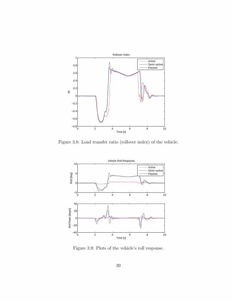
0 2 4 6 8 10−0.8
−0.6
−0.4
−0.2
0
0.2
0.4
0.6
0.8
1Rollover Index
Time [s]
RI
ActiveSemi−activePassive
Figure 3.8: Load transfer ratio (rollover index) of the vehicle.
0 2 4 6 8 10−5
0
5
10Vehicle Roll Response
Rol
l [de
g]
ActiveSemi−activePassive
0 2 4 6 8 10−40
−20
0
20
40
Rol
l Rat
e [d
eg/s
]
Time [s]
Figure 3.9: Plots of the vehicle’s roll response.
39
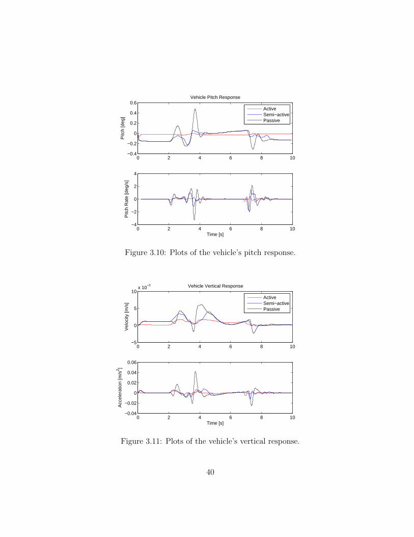
0 2 4 6 8 10−0.4
−0.2
0
0.2
0.4
0.6Vehicle Pitch Response
Pitc
h [d
eg]
ActiveSemi−activePassive
0 2 4 6 8 10−4
−2
0
2
4
Pitc
h R
ate
[deg
/s]
Time [s]
Figure 3.10: Plots of the vehicle’s pitch response.
0 2 4 6 8 10−5
0
5
10x 10
−3 Vehicle Vertical Response
Vel
ocity
[m/s
]
ActiveSemi−activePassive
0 2 4 6 8 10−0.04
−0.02
0
0.02
0.04
0.06
Time [s]
Acc
eler
atio
n [m
/s2 ]
Figure 3.11: Plots of the vehicle’s vertical response.
40
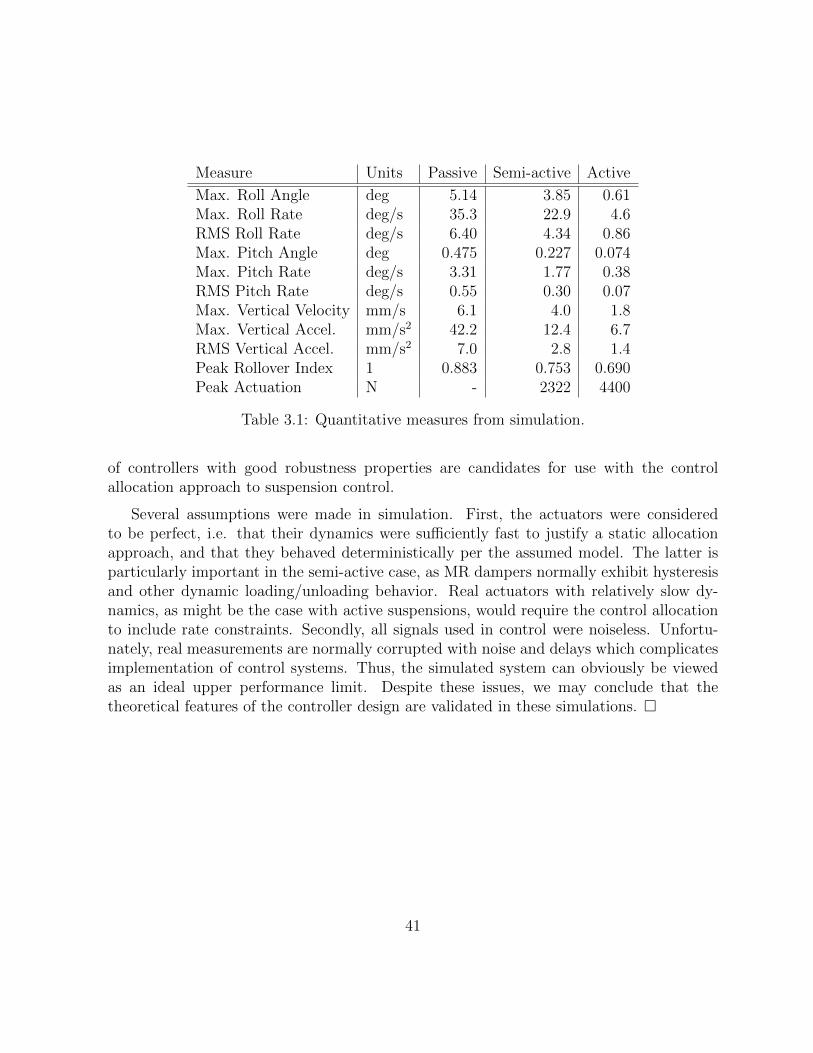
Measure Units Passive Semi-active Active
Max. Roll Angle deg 5.14 3.85 0.61Max. Roll Rate deg/s 35.3 22.9 4.6RMS Roll Rate deg/s 6.40 4.34 0.86Max. Pitch Angle deg 0.475 0.227 0.074Max. Pitch Rate deg/s 3.31 1.77 0.38RMS Pitch Rate deg/s 0.55 0.30 0.07Max. Vertical Velocity mm/s 6.1 4.0 1.8Max. Vertical Accel. mm/s2 42.2 12.4 6.7RMS Vertical Accel. mm/s2 7.0 2.8 1.4Peak Rollover Index 1 0.883 0.753 0.690Peak Actuation N - 2322 4400
Table 3.1: Quantitative measures from simulation.
of controllers with good robustness properties are candidates for use with the controlallocation approach to suspension control.
Several assumptions were made in simulation. First, the actuators were consideredto be perfect, i.e. that their dynamics were sufficiently fast to justify a static allocationapproach, and that they behaved deterministically per the assumed model. The latter isparticularly important in the semi-active case, as MR dampers normally exhibit hysteresisand other dynamic loading/unloading behavior. Real actuators with relatively slow dy-namics, as might be the case with active suspensions, would require the control allocationto include rate constraints. Secondly, all signals used in control were noiseless. Unfortu-nately, real measurements are normally corrupted with noise and delays which complicatesimplementation of control systems. Thus, the simulated system can obviously be viewedas an ideal upper performance limit. Despite these issues, we may conclude that thetheoretical features of the controller design are validated in these simulations.
41
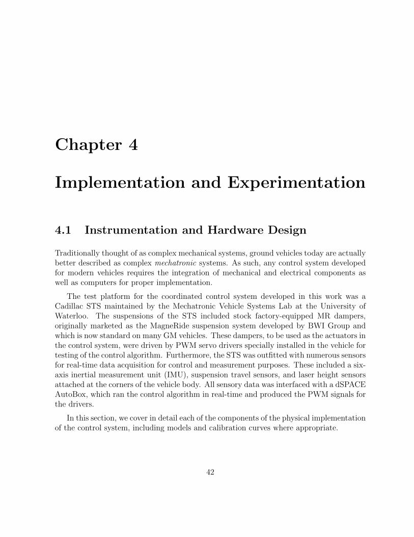
Chapter 4
Implementation and Experimentation
4.1 Instrumentation and Hardware Design
Traditionally thought of as complex mechanical systems, ground vehicles today are actuallybetter described as complex mechatronic systems. As such, any control system developedfor modern vehicles requires the integration of mechanical and electrical components aswell as computers for proper implementation.
The test platform for the coordinated control system developed in this work was aCadillac STS maintained by the Mechatronic Vehicle Systems Lab at the University ofWaterloo. The suspensions of the STS included stock factory-equipped MR dampers,originally marketed as the MagneRide suspension system developed by BWI Group andwhich is now standard on many GM vehicles. These dampers, to be used as the actuators inthe control system, were driven by PWM servo drivers specially installed in the vehicle fortesting of the control algorithm. Furthermore, the STS was outfitted with numerous sensorsfor real-time data acquisition for control and measurement purposes. These included a six-axis inertial measurement unit (IMU), suspension travel sensors, and laser height sensorsattached at the corners of the vehicle body. All sensory data was interfaced with a dSPACEAutoBox, which ran the control algorithm in real-time and produced the PWM signals forthe drivers.
In this section, we cover in detail each of the components of the physical implementationof the control system, including models and calibration curves where appropriate.
42
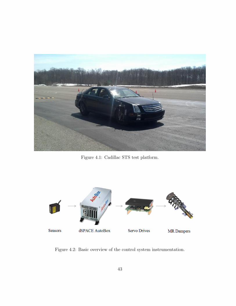
Figure 4.1: Cadillac STS test platform.
Figure 4.2: Basic overview of the control system instrumentation.
43
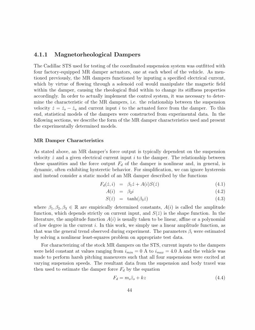
4.1.1 Magnetorheological Dampers
The Cadillac STS used for testing of the coordinated suspension system was outfitted withfour factory-equipped MR damper actuators, one at each wheel of the vehicle. As men-tioned previously, the MR dampers functioned by inputing a specified electrical current,which by virtue of flowing through a solenoid coil would manipulate the magnetic fieldwithin the damper, causing the rheological fluid within to change its stiffness propertiesaccordingly. In order to actually implement the control system, it was necessary to deter-mine the characteristic of the MR dampers, i.e. the relationship between the suspensionvelocity z = zs − zu and current input i to the actuated force from the damper. To thisend, statistical models of the dampers were constructed from experimental data. In thefollowing sections, we describe the form of the MR damper characteristics used and presentthe experimentally determined models.
MR Damper Characteristics
As stated above, an MR damper’s force output is typically dependent on the suspensionvelocity z and a given electrical current input i to the damper. The relationship betweenthese quantities and the force output Fd of the damper is nonlinear and, in general, isdynamic, often exhibiting hysteretic behavior. For simplification, we can ignore hysteresisand instead consider a static model of an MR damper described by the functions
Fd(z, i) = β1z + A(i)S(z) (4.1)
A(i) = β2i (4.2)
S(z) = tanh(β3z) (4.3)
where β1, β2, β3 ∈ R are empirically determined constants, A(i) is called the amplitudefunction, which depends strictly on current input, and S(z) is the shape function. In theliterature, the amplitude function A(i) is usually taken to be linear, affine or a polynomialof low degree in the current i. In this work, we simply use a linear amplitude function, asthat was the general trend observed during experiment. The parameters βi were estimatedby solving a nonlinear least-squares problem on appropriate test data.
For characterizing of the stock MR dampers on the STS, current inputs to the damperswere held constant at values ranging from imin = 0 A to imax = 4.0 A and the vehicle wasmade to perform harsh pitching maneuvers such that all four suspensions were excited atvarying suspension speeds. The resultant data from the suspension and body travel wasthen used to estimate the damper force Fd by the equation
Fd = mszs + kz (4.4)
44
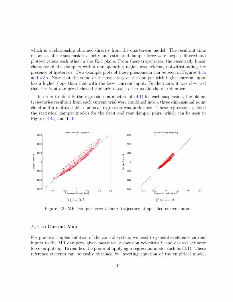
which is a relationship obtained directly from the quarter-car model. The resultant timeresponses of the suspension velocity and estimated damper force were lowpass filtered andplotted versus each other in the Fd-z plane. From these trajectories, the essentially linearcharacter of the dampers within our operating region was evident, notwithstanding thepresence of hysteresis. Two example plots of these phenomena can be seen in Figures 4.3aand 4.3b. Note that the trend of the trajectory of the damper with higher current inputhas a higher slope than that with the lesser current input. Furthermore, it was observedthat the front dampers behaved similarly to each other as did the rear dampers.
In order to identify the regression parameters of (4.1) for each suspension, the planartrajectories resultant from each current trial were combined into a three dimensional pointcloud and a multivariable nonlinear regression was performed. These regressions yieldedthe statistical damper models for the front and rear damper pairs, which can be seen inFigures 4.4a, and 4.4b.
−0.4 −0.2 0 0.2 0.4 0.6−3000
−2000
−1000
0
1000
2000
3000
Suspension Velocity [m/s]
Dam
per
For
ce [N
]
Force−Velocity Trajectory
(a) i = 0 A
−0.4 −0.2 0 0.2 0.4 0.6−3000
−2000
−1000
0
1000
2000
3000
Suspension Velocity [m/s]
Dam
per
For
ce [N
]
Force−Velocity Trajectory
(b) i = 4 A
Figure 4.3: MR Damper force-velocity trajectory at specified current input.
Fd-z to Current Map
For practical implementation of the control system, we need to generate reference currentinputs to the MR dampers, given measured suspension velocities zi and desired actuatorforce outputs ui. Herein lies the power of applying a regression model such as (4.1). Thesereference currents can be easily obtained by inverting equation of the empirical model,
45
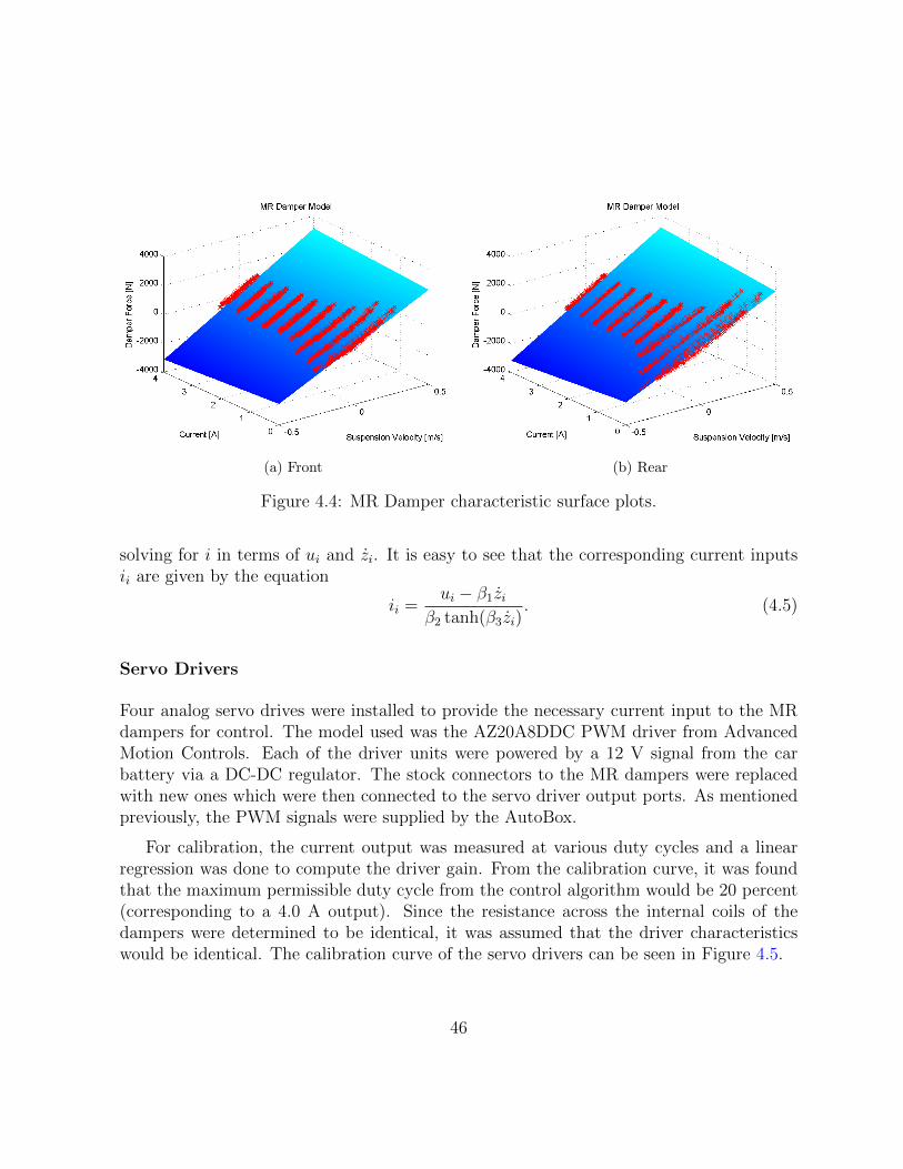
(a) Front (b) Rear
Figure 4.4: MR Damper characteristic surface plots.
solving for i in terms of ui and zi. It is easy to see that the corresponding current inputsii are given by the equation
ii =ui − β1zi
β2 tanh(β3zi). (4.5)
Servo Drivers
Four analog servo drives were installed to provide the necessary current input to the MRdampers for control. The model used was the AZ20A8DDC PWM driver from AdvancedMotion Controls. Each of the driver units were powered by a 12 V signal from the carbattery via a DC-DC regulator. The stock connectors to the MR dampers were replacedwith new ones which were then connected to the servo driver output ports. As mentionedpreviously, the PWM signals were supplied by the AutoBox.
For calibration, the current output was measured at various duty cycles and a linearregression was done to compute the driver gain. From the calibration curve, it was foundthat the maximum permissible duty cycle from the control algorithm would be 20 percent(corresponding to a 4.0 A output). Since the resistance across the internal coils of thedampers were determined to be identical, it was assumed that the driver characteristicswould be identical. The calibration curve of the servo drivers can be seen in Figure 4.5.
46

0 5 10 15 20 250
1
2
3
4
5
6Current Driver Characteristic
Duty Cycle (%)
Cur
rent
Out
put
y = 0.2098x
DataModel
Figure 4.5: Servo driver calibration curve.
4.1.2 Sensors
6-Axis Inertial Measurement Unit (IMU)
The RT2500 6-axis IMU from Oxford Technical Solutions installed on the STS enabledthe direct measurement of the linear velocities and accelerations along all principle axes,as well as roll, pitch, and yaw rates. For the purposes of coodinated suspension control,only the lateral and vertical accelerations ay and az, and the three angular velocities wererequired for feedback, to be used in the high-level controllers. The IMU internally used acombination of measurements from inertial sensors (accelerometers) and GPS with Kalmanfiltering for processing. The signal outputs from the IMU were interfaced directly with thedSPACE AutoBox via CAN inputs for use in the control algorithm.
Suspension Travel Sensors
Each individual suspension on the STS is equipped with stock linear variable differentialtransformers (LDVTs) for measuring the suspension travels at each wheel. For use in thecoodinated control system, the stock connectors were replaced so that the analog outputsignals from each sensor were available for feedback. The suspension sensors were powered
47
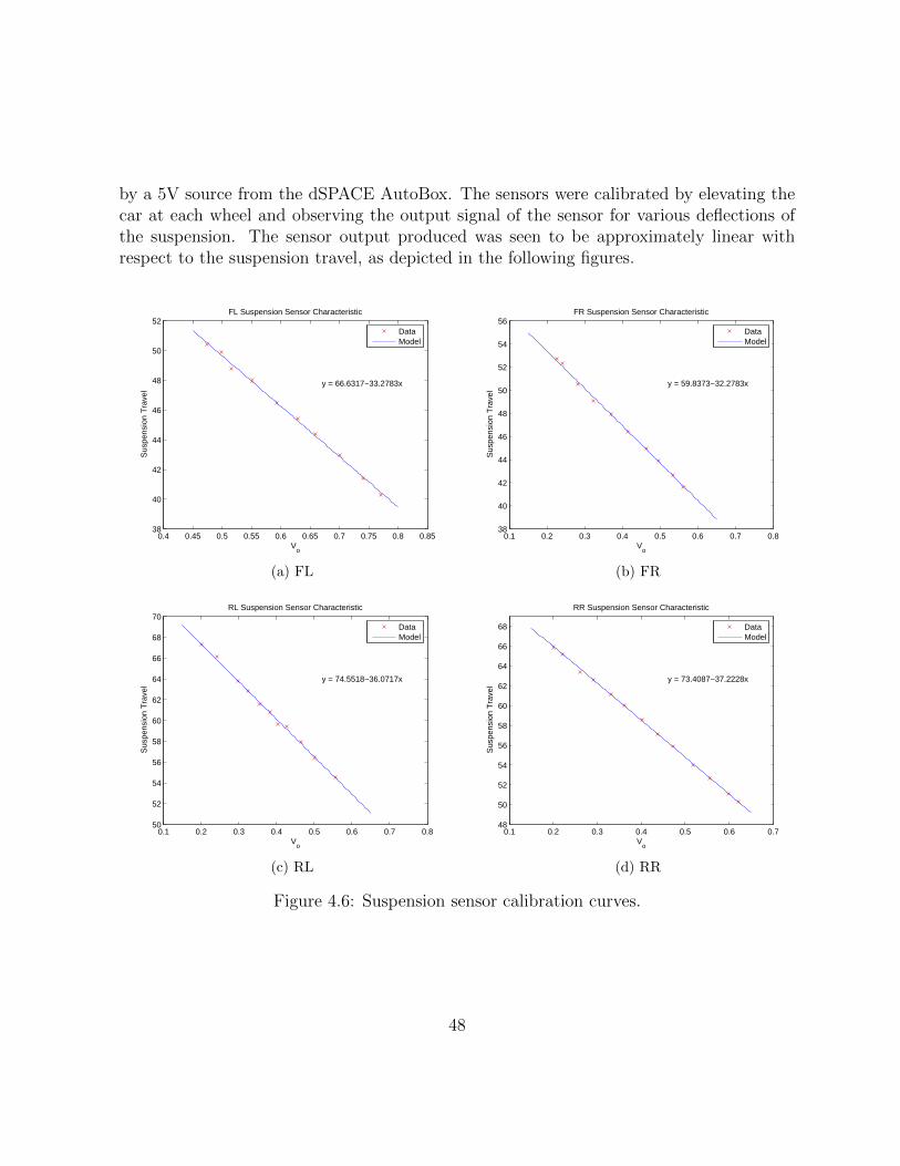
by a 5V source from the dSPACE AutoBox. The sensors were calibrated by elevating thecar at each wheel and observing the output signal of the sensor for various deflections ofthe suspension. The sensor output produced was seen to be approximately linear withrespect to the suspension travel, as depicted in the following figures.
0.4 0.45 0.5 0.55 0.6 0.65 0.7 0.75 0.8 0.8538
40
42
44
46
48
50
52FL Suspension Sensor Characteristic
Vo
Sus
pens
ion
Tra
vel
y = 66.6317−33.2783x
DataModel
(a) FL
0.1 0.2 0.3 0.4 0.5 0.6 0.7 0.838
40
42
44
46
48
50
52
54
56FR Suspension Sensor Characteristic
Vo
Sus
pens
ion
Tra
vel
y = 59.8373−32.2783x
DataModel
(b) FR
0.1 0.2 0.3 0.4 0.5 0.6 0.7 0.850
52
54
56
58
60
62
64
66
68
70RL Suspension Sensor Characteristic
Vo
Sus
pens
ion
Tra
vel
y = 74.5518−36.0717x
DataModel
(c) RL
0.1 0.2 0.3 0.4 0.5 0.6 0.748
50
52
54
56
58
60
62
64
66
68
RR Suspension Sensor Characteristic
Vo
Sus
pens
ion
Tra
vel
y = 73.4087−37.2228x
DataModel
(d) RR
Figure 4.6: Suspension sensor calibration curves.
48
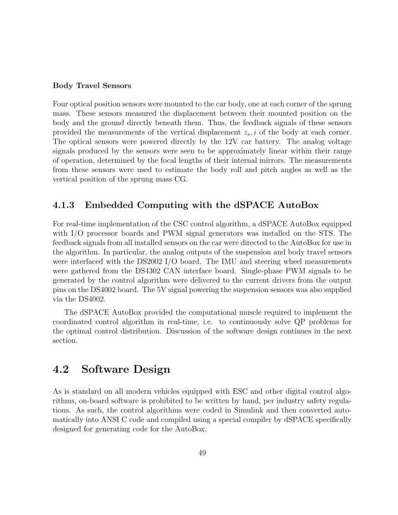
Body Travel Sensors
Four optical position sensors were mounted to the car body, one at each corner of the sprungmass. These sensors measured the displacement between their mounted position on thebody and the ground directly beneath them. Thus, the feedback signals of these sensorsprovided the measurements of the vertical displacement zs, i of the body at each corner.The optical sensors were powered directly by the 12V car battery. The analog voltagesignals produced by the sensors were seen to be approximately linear within their rangeof operation, determined by the focal lengths of their internal mirrors. The measurementsfrom these sensors were used to estimate the body roll and pitch angles as well as thevertical position of the sprung mass CG.
4.1.3 Embedded Computing with the dSPACE AutoBox
For real-time implementation of the CSC control algorithm, a dSPACE AutoBox equippedwith I/O processor boards and PWM signal generators was installed on the STS. Thefeedback signals from all installed sensors on the car were directed to the AutoBox for use inthe algorithm. In particular, the analog outputs of the suspension and body travel sensorswere interfaced with the DS2002 I/O board. The IMU and steering wheel measurementswere gathered from the DS4302 CAN interface board. Single-phase PWM signals to begenerated by the control algorithm were delivered to the current drivers from the outputpins on the DS4002 board. The 5V signal powering the suspension sensors was also suppliedvia the DS4002.
The dSPACE AutoBox provided the computational muscle required to implement thecoordinated control algorithm in real-time, i.e. to continuously solve QP problems forthe optimal control distribution. Discussion of the software design continues in the nextsection.
4.2 Software Design
As is standard on all modern vehicles equipped with ESC and other digital control algo-rithms, on-board software is prohibited to be written by hand, per industry safety regula-tions. As such, the control algorithms were coded in Simulink and then converted auto-matically into ANSI C code and compiled using a special compiler by dSPACE specificallydesigned for generating code for the AutoBox.
49

The software architecture of the control system consisted of four parts: the InputProcessing block, for reading and transforming sensor data, the High-Level Controllers, forgenerating the virtual control signals, the Control Allocator, for optimal distribution of theactuator controls, and the Output Processing block, for generating reference currents andduty cycles for the servo drivers. In this section, we describe each of these four modules indetail.
4.2.1 Input Processing and Estimation
The Input Processing block took as input the vector Input of all measured signals from thesensors deployed on the vehicle. The module had three functions: to convert all measuredsignals into the required units, to estimate all other required quantities from the measureddata, and to compute the adaptation parameters α.
The inputs to the dSPACE AutoBox, being analog voltage readings from the suspensionand body travel sensors, needed to be converted into appropriate units for use with the con-trol algorithm. The analog signals from the DS2002 board were read through a specializedDS2002 32-channel Multiplexer ADC function. Then, using the regression models of thesensors presented in the previous sections, the analog inputs were transformed into the nec-essary kinematic data. Data from the IMU interfaced with the DS4302 CAN bus was readthrough RTI CAN Receive Message functions. As these signals were digital, conversionsof these measurements into appropriate units was done using simple gain functions.
From the sensory data, other quantities necessary for control of the vehicle could becomputed or estimated. Signal noise was removed by using discrete first-order filters(weighted moving average filters). In particular, the suspension and body travel data werepassed through triangular smoothing filters to remove noise and were then sent throughdiscrete derivative blocks to obtain their velocities. The roll and pitch angles as well as thedisplacement of the sprung mass CG were estimated from the measured body travel data.
Computation of the adaptation parameters for roll and pitch control was performedin the way specified in the previous chapter. All measured and estimated quantities werepassed as output from the block in a single vector InputP for use in other modules. Thevector of adaptivity parameters Alpha was also output for use in the control allocationblock.
50

4.2.2 High-Level Controllers
The High-Level Controller module took as input the vector of processed inputs and esti-mated quantities InputP, and output the vector of virtual control signals v. This vectorcontained the two generalized moments Mx and My, the generalized CG force Fz, andthe four localized suspension controls u0. The roll moment Mx was defined by the slidingmode control law (3.4) and the pitch moment My and vertical CG force Fz were definedby the control law (3.16). The localized suspension controls were defined by the hybridskyhook-groundhook semi-active control law. The vector v of these virtual control signalswas output to the control allocation module for distribution.
4.2.3 Control Allocator
The Control Allocator module took as input the vector of processed inputs InputP, thevector of virtual control signals v, the vector of adaptation parameters Alpha, and a vectorof boolean values Fault. The purpose of the control allocator was to solve the constrainedQP problem (3.41) for the actuator forces u. This was accomplished in two parts: thecomputation of all necessary quantities for the optimization problem, and the real-timesolution of the quadratic program.
The quantities necessary to define the optimization problem included the weightingmatrices Wv and Wu, and the control effectiveness matrix B in order to define the objectivefunction, as well as the vector of upper bounds u and lower bounds u for the actuatorcontrols, defining the set of feasible values U . In particular, the weighting matrix Wv
was computed dynamically using the adaptivity parameters in the vector Alpha, and theactuator bounds were computed using the statistical MR damper characteristics. TheFault array, consisting of four boolean values encoded information on the fault state ofthe actuators. If for each true value in Fault, the corresponding actuator was removedfrom the optimization process. This was done by simply setting the corresponding columnsof B and elements of u0 to zero.
The solution of the quadratic programming problem was performed using the QCAT
toolbox developed by Harkegard [9]. The specific function used was a modified version ofwls alloc, which applies an active set algorithm for solution of control allocation problemsdefined by quadratic programs. Modifications were made to the code so that it couldcompile on the dSPACE AutoBox. In particular, the reliance on dynamically-sized arraysand logical indexing were removed. The output of the optimization process was the vectoru containing the four actuator controls, and the quantity qpIter which counted the numberof iterations required by the solver to find the optimal solution.
51
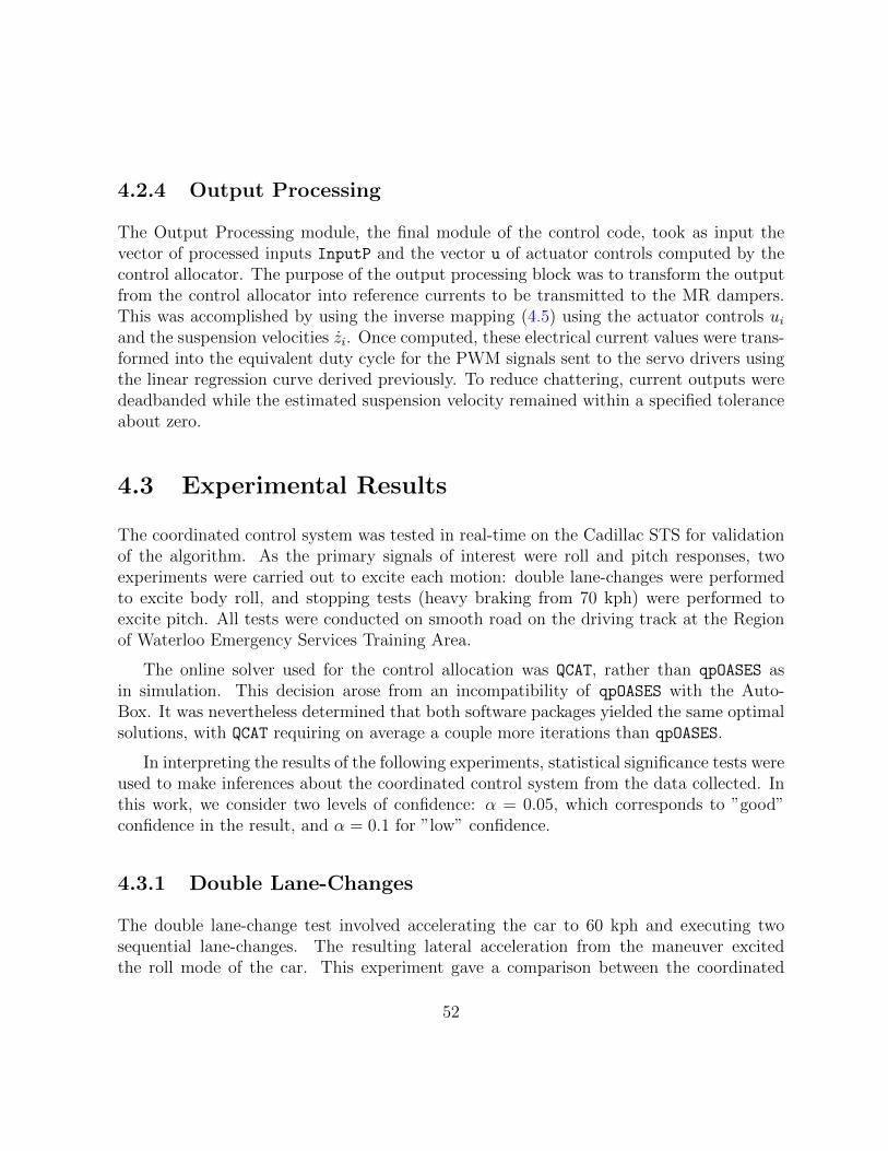
4.2.4 Output Processing
The Output Processing module, the final module of the control code, took as input thevector of processed inputs InputP and the vector u of actuator controls computed by thecontrol allocator. The purpose of the output processing block was to transform the outputfrom the control allocator into reference currents to be transmitted to the MR dampers.This was accomplished by using the inverse mapping (4.5) using the actuator controls uiand the suspension velocities zi. Once computed, these electrical current values were trans-formed into the equivalent duty cycle for the PWM signals sent to the servo drivers usingthe linear regression curve derived previously. To reduce chattering, current outputs weredeadbanded while the estimated suspension velocity remained within a specified toleranceabout zero.
4.3 Experimental Results
The coordinated control system was tested in real-time on the Cadillac STS for validationof the algorithm. As the primary signals of interest were roll and pitch responses, twoexperiments were carried out to excite each motion: double lane-changes were performedto excite body roll, and stopping tests (heavy braking from 70 kph) were performed toexcite pitch. All tests were conducted on smooth road on the driving track at the Regionof Waterloo Emergency Services Training Area.
The online solver used for the control allocation was QCAT, rather than qpOASES asin simulation. This decision arose from an incompatibility of qpOASES with the Auto-Box. It was nevertheless determined that both software packages yielded the same optimalsolutions, with QCAT requiring on average a couple more iterations than qpOASES.
In interpreting the results of the following experiments, statistical significance tests wereused to make inferences about the coordinated control system from the data collected. Inthis work, we consider two levels of confidence: α = 0.05, which corresponds to ”good”confidence in the result, and α = 0.1 for ”low” confidence.
4.3.1 Double Lane-Changes
The double lane-change test involved accelerating the car to 60 kph and executing twosequential lane-changes. The resulting lateral acceleration from the maneuver excitedthe roll mode of the car. This experiment gave a comparison between the coordinated
52
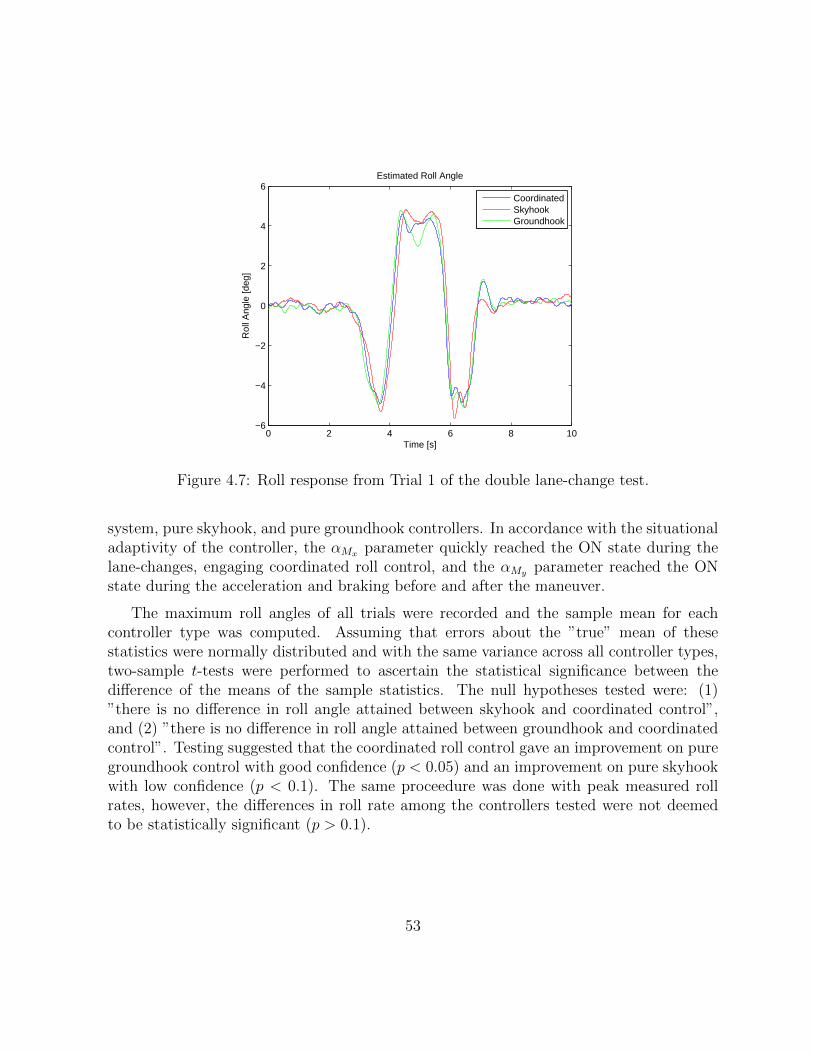
0 2 4 6 8 10−6
−4
−2
0
2
4
6
Time [s]
Rol
l Ang
le [d
eg]
Estimated Roll Angle
CoordinatedSkyhookGroundhook
Figure 4.7: Roll response from Trial 1 of the double lane-change test.
system, pure skyhook, and pure groundhook controllers. In accordance with the situationaladaptivity of the controller, the αMx parameter quickly reached the ON state during thelane-changes, engaging coordinated roll control, and the αMy parameter reached the ONstate during the acceleration and braking before and after the maneuver.
The maximum roll angles of all trials were recorded and the sample mean for eachcontroller type was computed. Assuming that errors about the ”true” mean of thesestatistics were normally distributed and with the same variance across all controller types,two-sample t-tests were performed to ascertain the statistical significance between thedifference of the means of the sample statistics. The null hypotheses tested were: (1)”there is no difference in roll angle attained between skyhook and coordinated control”,and (2) ”there is no difference in roll angle attained between groundhook and coordinatedcontrol”. Testing suggested that the coordinated roll control gave an improvement on puregroundhook control with good confidence (p < 0.05) and an improvement on pure skyhookwith low confidence (p < 0.1). The same proceedure was done with peak measured rollrates, however, the differences in roll rate among the controllers tested were not deemedto be statistically significant (p > 0.1).
53
0 2 4 6 8 10−40
−30
−20
−10
0
10
20
30
Time [s]
Rol
l Rat
e [d
eg/s
]
Estimated Roll Rate
CoordinatedSkyhookGroundhook
Figure 4.8: Roll rate response from Trial 1 of the double lane-change test.
0 2 4 6 8 100
0.2
0.4
0.6
0.8
1
1.2
1.4
Time [s]
Alp
ha
Adaptation Parameters − Dbl Lane Change Test
AlphaRAlphaP
Figure 4.9: Adaptivity parameters in a double lane-change. The pitch parameter activatesat the end when breaking is initiated.
54
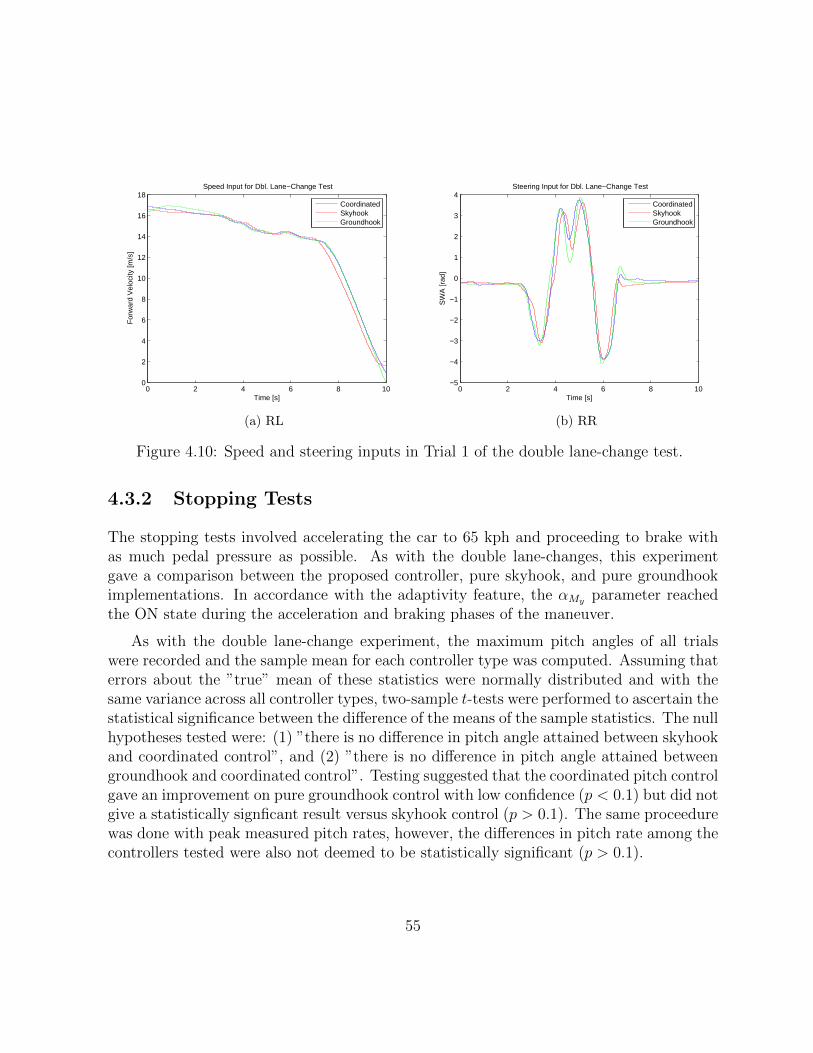
0 2 4 6 8 100
2
4
6
8
10
12
14
16
18
Time [s]
For
war
d V
eloc
ity [m
/s]
Speed Input for Dbl. Lane−Change Test
CoordinatedSkyhookGroundhook
(a) RL
0 2 4 6 8 10−5
−4
−3
−2
−1
0
1
2
3
4
Time [s]
SW
A [r
ad]
Steering Input for Dbl. Lane−Change Test
CoordinatedSkyhookGroundhook
(b) RR
Figure 4.10: Speed and steering inputs in Trial 1 of the double lane-change test.
4.3.2 Stopping Tests
The stopping tests involved accelerating the car to 65 kph and proceeding to brake withas much pedal pressure as possible. As with the double lane-changes, this experimentgave a comparison between the proposed controller, pure skyhook, and pure groundhookimplementations. In accordance with the adaptivity feature, the αMy parameter reachedthe ON state during the acceleration and braking phases of the maneuver.
As with the double lane-change experiment, the maximum pitch angles of all trialswere recorded and the sample mean for each controller type was computed. Assuming thaterrors about the ”true” mean of these statistics were normally distributed and with thesame variance across all controller types, two-sample t-tests were performed to ascertain thestatistical significance between the difference of the means of the sample statistics. The nullhypotheses tested were: (1) ”there is no difference in pitch angle attained between skyhookand coordinated control”, and (2) ”there is no difference in pitch angle attained betweengroundhook and coordinated control”. Testing suggested that the coordinated pitch controlgave an improvement on pure groundhook control with low confidence (p < 0.1) but did notgive a statistically signficant result versus skyhook control (p > 0.1). The same proceedurewas done with peak measured pitch rates, however, the differences in pitch rate among thecontrollers tested were also not deemed to be statistically significant (p > 0.1).
55

Measure Units Skyhook Groundhook Coordinated
Max. Roll Angle deg 5.654 5.103 4.907RMS Roll Angle deg 2.420 2.343 2.327Max. Roll Rate deg/s 35.76 31.16 34.20RMS Roll Rate deg/s 7.125 6.791 6.764
Table 4.1: Quantitative measures from Trial 1 of the double lane-change test.
Measure Units Skyhook Groundhook Coordinated
Max. Roll Angle deg 5.232 5.068 4.858RMS Roll Angle deg 2.368 2.183 2.157Max. Roll Rate deg/s 24.72 25.50 28.25RMS Roll Rate deg/s 6.528 6.032 6.536
Table 4.2: Quantitative measures from Trial 2 of the double lane-change test.
Measure Units Skyhook Groundhook Coordinated
Max. Pitch Angle deg 2.290 2.610 2.140RMS Pitch Angle deg 1.387 1.484 1.344Max. Pitch Rate deg/s 13.77 10.80 11.06RMS Pitch Rate deg/s 1.938 2.193 1.937
Table 4.3: Quantitative measures from Trial 1 of the stopping test.
Measure Units Skyhook Groundhook Coordinated
Max. Pitch Angle deg 1.936 2.474 1.810RMS Pitch Angle deg 1.326 1.389 1.283Max. Pitch Rate deg/s 9.530 12.57 12.83RMS Pitch Rate deg/s 3.102 2.555 2.882
Table 4.4: Quantitative measures from Trial 2 of the stopping test.
Measure Units xsky σ2sky xgnd σ2
gnd xCSC σ2CSC
Max. Roll Angle deg 5.443 8.9 · 10−2 5.085 6.4 · 10−4 4.883 1.2 · 10−3
Max. Pitch Angle deg 2.113 6.3 · 10−2 2.542 9.4 · 10−3 1.975 5.2 · 10−2
Max. Roll Rate deg/s 30.24 60.96 28.33 16.02 31.22 17.70Max. Pitch Rate deg/s 11.65 8.99 11.68 1.566 11.94 1.566
Table 4.5: Sample means and variances from test data.
56
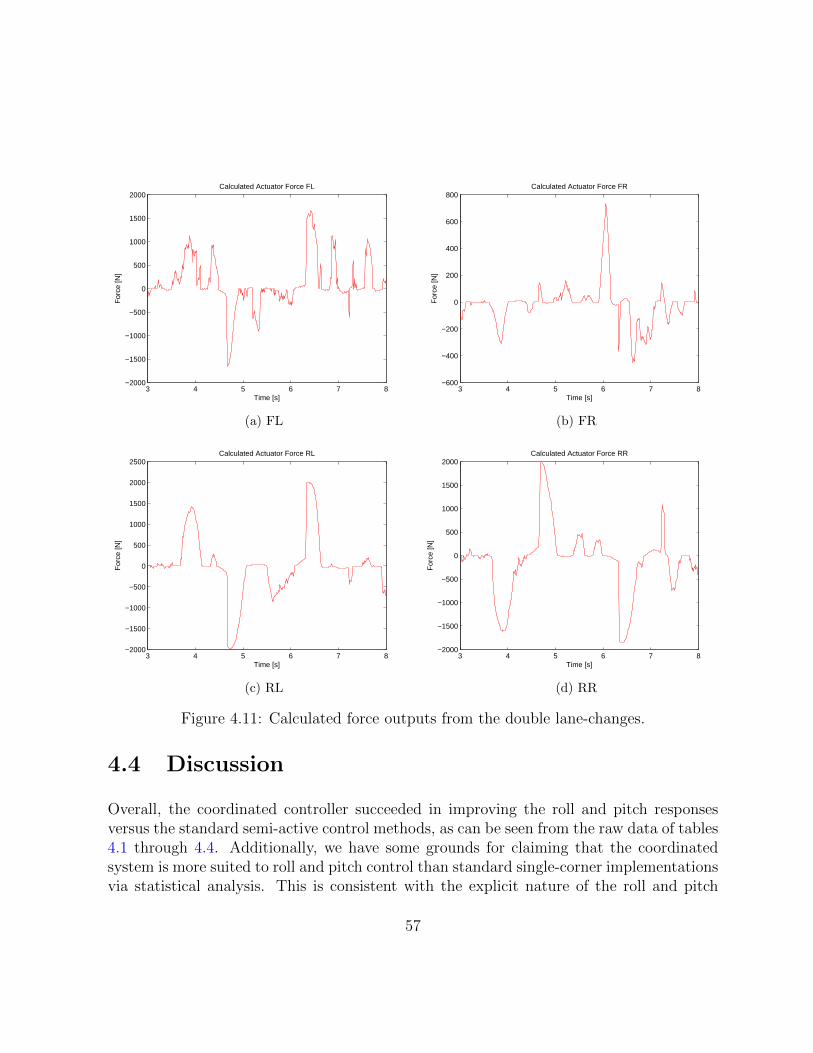
3 4 5 6 7 8−2000
−1500
−1000
−500
0
500
1000
1500
2000Calculated Actuator Force FL
Time [s]
For
ce [N
]
(a) FL
3 4 5 6 7 8−600
−400
−200
0
200
400
600
800Calculated Actuator Force FR
Time [s]
For
ce [N
]
(b) FR
3 4 5 6 7 8−2000
−1500
−1000
−500
0
500
1000
1500
2000
2500Calculated Actuator Force RL
Time [s]
For
ce [N
]
(c) RL
3 4 5 6 7 8−2000
−1500
−1000
−500
0
500
1000
1500
2000Calculated Actuator Force RR
Time [s]
For
ce [N
]
(d) RR
Figure 4.11: Calculated force outputs from the double lane-changes.
4.4 Discussion
Overall, the coordinated controller succeeded in improving the roll and pitch responsesversus the standard semi-active control methods, as can be seen from the raw data of tables4.1 through 4.4. Additionally, we have some grounds for claiming that the coordinatedsystem is more suited to roll and pitch control than standard single-corner implementationsvia statistical analysis. This is consistent with the explicit nature of the roll and pitch
57

0 2 4 6 8 10−3
−2
−1
0
1
2
3
Time [s]
Pitc
h A
ngle
[deg
]
Estimated Pitch Angle
CoordinatedSkyhookGroundhook
Figure 4.12: Pitch response from Trial 1 of the stopping test.
0 2 4 6 8 10−15
−10
−5
0
5
10
15
Time [s]
Pitc
h R
ate
[deg
/s]
Estimated Pitch Rate
CoordinatedSkyhookGroundhook
Figure 4.13: Pitch rate response from Trial 1 of the stopping test.
58
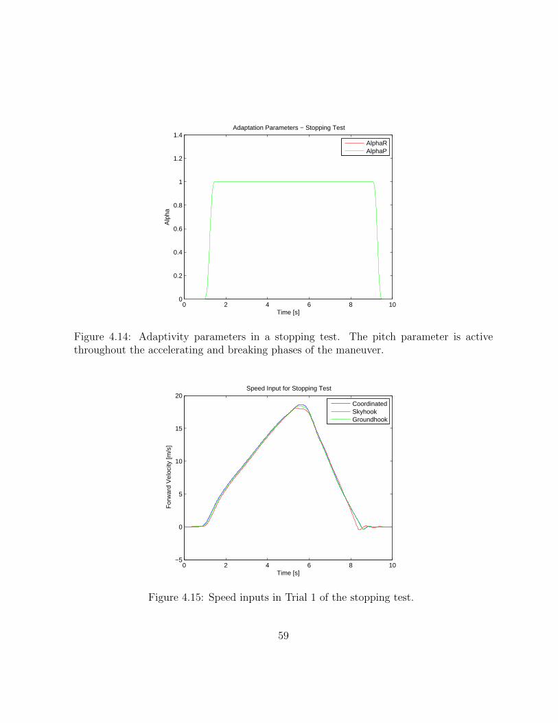
0 2 4 6 8 100
0.2
0.4
0.6
0.8
1
1.2
1.4
Time [s]
Alp
ha
Adaptation Parameters − Stopping Test
AlphaRAlphaP
Figure 4.14: Adaptivity parameters in a stopping test. The pitch parameter is activethroughout the accelerating and breaking phases of the maneuver.
0 2 4 6 8 10−5
0
5
10
15
20
Time [s]
For
war
d V
eloc
ity [m
/s]
Speed Input for Stopping Test
CoordinatedSkyhookGroundhook
Figure 4.15: Speed inputs in Trial 1 of the stopping test.
59

0 2 4 6 8 10−1500
−1000
−500
0
500
1000
1500Calculated Actuator Force FL
Time [s]
For
ce [N
]
(a) FL
0 2 4 6 8 10−800
−600
−400
−200
0
200
400
600
800Calculated Actuator Force FR
Time [s]
For
ce [N
]
(b) FR
0 2 4 6 8 10−1500
−1000
−500
0
500
1000
1500
2000
2500Calculated Actuator Force RL
Time [s]
For
ce [N
]
(c) RL
0 2 4 6 8 10−1500
−1000
−500
0
500
1000
1500
2000Calculated Actuator Force RR
Time [s]
For
ce [N
]
(d) RR
Figure 4.16: Calculated force outputs from the stopping tests.
control in the optimization procedure, versus the supposed indirect control of these degreesof freedom via single-corner control.
As a handling-based controller, the groundhook method performed better than skyhookin the double lane-change test in terms of both roll angle and roll rate. The coordinatedcontroller matched groundhook in this case for the most part, with slight improvement inroll angle control. Notably, the peak roll rate of the vehicle with the coodinated controller
60

Measure Controller 1 Controller 2 t-score p-value Reject H0?
Max. Roll Angle Coordinated Skyhook 2.6405 0.0593 Yes*Groundhook 6.7195 0.0214 Yes
Max. Pitch Angle Coordinated Skyhook 0.5698 0.6263 NoGroundhook 0.5698 0.0865 Yes*
Max. Roll Rate Coordinated Skyhook 0.1569 0.5318 NoGroundhook 0.7050 0.5538 No
Max. Pitch Rate Coordinated Skyhook 0.1284 0.9096 NoGroundhook 0.2077 0.8547 No
Table 4.6: Student’s t-test results and p-values. An asterisk denotes meeting the lowconfidence threshold α = 0.1.
is more comparable to the skyhook response, however the RMS of the roll rate with thecoordinated controller is more similar to the groundhook response. In terms of maximumroll angle, the t-tests showed that the coordinated system faired better than groundhookcontrol with good confidence (p < 0.05). Improvement versus skyhook control was seen aswell, however with a lower confidence.
According to the data, the skyhook controller performed better than the groundhookcontroller in the stopping test. This is probably because the pitch motion in the stoppingtest is due more to pure sprung mass vibration rather than wheel motion or load transfer.In pitch control, the coodinated strategy matched the skyhook response with a slightimprovement in the angular and rate responses. Moreover, the maximum pitch rate ofthe vehicle with the coodinated controller gave an improvement on the skyhook control,matching more closely the groundhook response, though still slightly higher. In terms ofmaximum pitch angle, the t-tests showed that the coordinated system faired better thangroundhook control with low confidence (p < 0.1), but not versus skyhook control.
From the data, we see that the coodinated controller achieves responses comparableto both skyhook and groundhook depending on the situation. As such, the coordinatedsuspension control system can be thought of as a form of hybrid control. Moreover, thedata appears to suggest that the explicit inclusion of roll and pitch control in the controllerdesign allows for improvement of these responses, as hypothesized in [4].
As we have seen in the previous section, the control system designed in this worksucceeded in improving the pitch and roll responses of the vehicle system tested versusthe purely passive case. In the current implementation, the results do not quite scale tothose expected from simulation. This can be for a number of reasons, among them the
61
loss of the ”perfect actuator” assumption, the presence of noises in the signals and theconsequent effects of delays from filtering. All of these issues, conspicuously absent fromthe simulations, were present in the real-world system and hence degraded performance.
Simulations assumed that the MR dampers behaved precisely like the statistical models(4.1), and that the suspension velocities were perfectly known. The damper forces calcu-lated in simulation were therefore at best approximate, as it was observed that the realMR dampers exhibited hysteresis. Signal noise, particularly in the suspension travel sen-sors, was prevalent. As the suspension travels needed to be differentiated to obtain theirvelocities, the signals needed to be strongly prefiltered. This resulted in a time delay of afew hundredths of a second, which in dynamic situations is rather significant, as vibrationsin the suspensions can occur at very high frequencies. No such delay was considered insimulation since filtering was unnecessary.
It must also be remembered that vehicle testing can be somewhat subjective. In testing,several practice runs were performed beforehand so that the driver could perform thetest maneuvers with relative consistency. This was particularly important for the doublelane-changes, being the more technical of the two chosen tests. Since the vehicle testswere performed by a human, slight discrepancies in the steering (double lane-changes) orapplied break pressure (stopping tests) between test runs constitute a probable source ofsystematic error. From Figures 4.10 and 4.15, we can see that the test runs performed arerelatively consistent. Additionally, environmental factors are a potential source of randomerror in the experiment. Though as the tests were performed on a sunny day with lowwind and on a dry track, this error could be considered negligible. These sources of errorcould be alleviated by substituting the human driver by a computer, and by testing in alarge, indoor facility.
The t-tests were performed in order to make more educated inferences from the test datagiven the presence of uncertainties in the system during testing. Overall, the statisticalanalysis suggested that the coordinated system controlled roll and pitch angles betterthan single-corner controllers, but with lower confidence than would be desired in somecases. Of note is that only two trials were performed for each maneuver. Repeating theexperiment with more trials could potentially bring the p-values of interest down to thedesired level. On the other hand, the low p-value in the coordinated vs. groundhook rollcontrol comparision might be attributable to the low sample variance in the groundhookcase. Performing more trials might increase the sample variance, thus increase the p-valueinto the low confidence range.
Finally, another issue was the test vehicle itself, in particular the stock MR dampers. Incharacterizing the dampers in 4.1.1, it was observed that the change in damping between
62
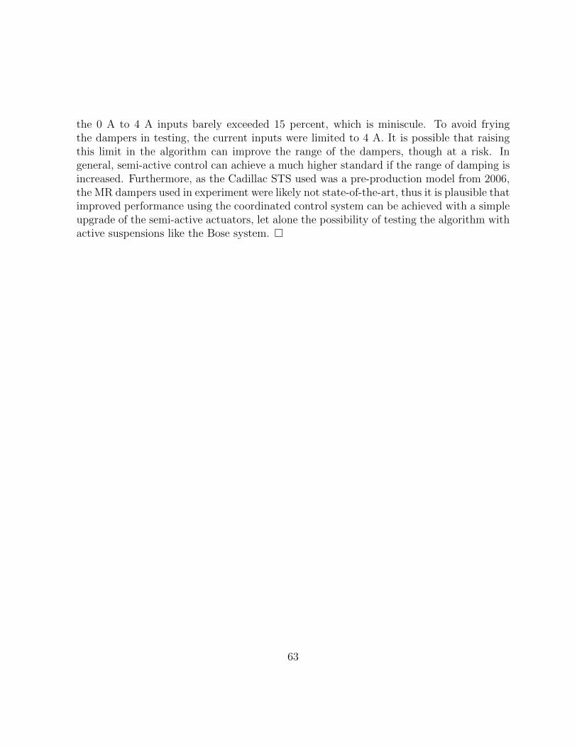
the 0 A to 4 A inputs barely exceeded 15 percent, which is miniscule. To avoid fryingthe dampers in testing, the current inputs were limited to 4 A. It is possible that raisingthis limit in the algorithm can improve the range of the dampers, though at a risk. Ingeneral, semi-active control can achieve a much higher standard if the range of damping isincreased. Furthermore, as the Cadillac STS used was a pre-production model from 2006,the MR dampers used in experiment were likely not state-of-the-art, thus it is plausible thatimproved performance using the coordinated control system can be achieved with a simpleupgrade of the semi-active actuators, let alone the possibility of testing the algorithm withactive suspensions like the Bose system.
63
Chapter 5
Conclusions and Future Work
5.1 Conclusions
Revisiting the central question of this thesis, whether we can generalize suspension control(particularly semi-active control) to encompass all vertical vehicle dynamics in a coordi-nated way, which would be integrable with modern ESC systems, we can affirmatively say”yes”. The coordinated suspension control system, or CSC, does exactly that throughthe application of control allocation techniques. Such a formulation has the advantage ofexplicitly designing the controller to improve roll and pitch responses, which is often notconsidered at all in suspension controllers, semi-active control laws in particular.
We have seen that the coordinated system improves the vehicle response compared topassive suspensions. As well, we have seen that the given implementation is comparableto other handling-oriented semi-active control strategies designed for a single-corner, likegroundhook control. The promise shown by this type of coordinated system is especiallyevident in the wake of the development of active suspensions, but may also find utilitywhen formulated with conventional semi-active adaptive actuators. Further developmentis required to optimize the CSC system, however, before it can be definitively stated thatit is superior to single-corner implementations.
5.2 Recommendations for Future Work
We conclude this work with some recommendations for future research and developmentbased on the experiences acquired during the course of this project.
64

Refining of Actuator Models
In section 4.1.1, the MR dampers on the Cadillac STS were characterized by fitting a staticstatistical model to experimental data. Owing to the approximate nature of these charac-teristics because of modeling errors and noisy data, some performance degradation was tobe expected. Therefore, more accurate models of the equipped dampers should improveperformance. Much exists already in the literature on the modeling of the dynamics ofMR dampers, many being variations on the well-known Bouc-Wen model. Ideally, one ortwo of the STS dampers should be removed from the car and tested in a lab with a forcegenerator to map out their characteristics in the most accurate way possible. Afterwards,the data can be fit to a possibly more complicated, dynamic model and the problem ofintegrating this new model with the control allocation can then be explored.
Improved Filtering and Estimation
Signal noise is an ever present annoyance in engineering systems and a primary source ofperformance degradation, and this system is no exception. Sources of noises in the controlsystem included both mechanical and electrical vibrations. In particular, the suspensiontravel sensors were quite noisy, and had to be heavily filtered for use in the algorithm.Research into sensor technology and filtering techniques could greatly impact performancegains. In order to sidestep the task of differentiating the suspension sensor signals, itmight be more appropriate to apply a rate linear encoder for direct measurement of thesuspension velocities, as the relative displacement of the suspensions themselves are notuseful, whereas the velocity is key to proper implementation of the algorithm. The primarydrawback to this is an increased cost of implementation.
In testing of the control system, multiple sensors were deployed for direct measurementof the required signals. For commercialization, the number of these sensors should beminimized. In particular, the body travel sensors are prime candidates for replacementvia estimation algorithms. Moreover, performance might be improved by use of parameterestimation modules to further account for parametric uncertainties.
Research into Active Suspension Systems
Simulation in section 3.3.1 suggests that the coordinated control of the suspensions candeliver complete regulation of the vertical dynamics to zero state, assuming a perfect setof actuators. It remains to develop a commercially available active suspension which can
65
deliver the power required for this task with the necessary bandwidth. When such anactuator can be fitted to a test vehicle, the active form of the control algorithm explored inthis thesis can be tested. In the case that the active actuators do not possess the requiredbandwidth, it might also be worthwhile to explore ideas of dynamic control allocation,which can incorporate the actuator dynamics into the control allocator design.
Integration and Testing with ESC Systems
As seen in the literature review, control allocation techniques have been applied to thedesign of ESC for yaw stabilization and the control of lateral acceleration. The controlallocation approach enables both coordinated control of the suspensions and yaw stabilitycontrol to be integrated into a single framework. The integration of yaw stability controland coordinated suspension control can be built into the control allocator. Redefining thevirtual control signals and the vector of actuator controls to include both suspension andmotor controls, we obtain a QP problem as with the standalone system, but of higherdimension. Though this presents a larger optimization problem, it is not nearly largeenough to be intractable and can therefore be solved online using an active-set algorithm.
Once integrated, the combination of motor and suspension controls would constitute arobust rollover prevention system, through the combined control of lateral acceleration, yawrate, and roll angle, the major factors in vehicle rollover. More generally, the integrationof these systems would bring one step closer the realization of a complete vehicle dynamicscontrol system.
66

Bibliography
[1] Daimler AG. Active body control, http://techcenter.mercedes-benz.com/ en
/abc/detail.html.
[2] A. Agrawal. Performance Improvement of Automotive Suspension Systems using In-erters and an Adaptive Controller. Master’s thesis, University of Waterloo, Waterloo,ON, Canada, 2013.
[3] A. Agrawal and A. Khajepour. A new adaptive controller for performance improve-ment of automotive suspension systems with MR dampers. SAE Intl. J. Passeng.Cars - Mech. Syst., 7(3), 2014.
[4] M. K. Binder and A. Khajepour. Optimal control allocation for coordinated suspensioncontrol. In Proc. of the American Control Conference 2014, Portland, OR, 2014.
[5] S. Boyd and L. Vandenberghe. Convex Optimization. Cambridge University Press,New York, 7th edition, 2009.
[6] Bose Corporation. Bose suspension system, http://www.bose.com/controller?url=/automotive/bose suspension/index.jsp.
[7] H. J. Ferreau. An Online Active Set Strategy for Fast Solution of Parametric QuadraticPrograms with Applications to Predictive Engine Control. Master’s thesis, UniversitatHeidelberg, Heidelberg, Germany, 2006.
[8] G. J. Forkenbrock, W. Garrot, M. Heitz, and B. C. O’Harra. A comprehensive ex-perimental examination of test maneuvers that may induce on-road, untripped, lightvehicle rollover - phase IV of NHTSAs light vehicle rollover research program. Tech-nical report, National Highway Traffic Safety Administration, 2002.
[9] O. Harkegard. Quadratic programming control allocation toolbox for MATLAB,http://research.harkegard.se/qcat/index.html.
67
[10] O. Harkegard. Efficient active set algorithms for solving constrained least squaresproblems in aircraft control allocation. In Proc. of the Conf. on Decision and Control2002, Las Vegas, NV, 2002.
[11] O. Harkegard. Backstepping and Control Allocation with Applications to Flight Con-trol. PhD thesis, Linkoping University, Linkoping, Sweden, 2003.
[12] O. Harkegard. Dynamic control allocation using quadratic programming. Journal ofGuidance, Control, and Dynamics, 27(6):1028–1034, 2004.
[13] R. Jazar. Vehicle Dynamics: Theory and Applications. Springer, New York, 2008.
[14] T. A. Johansen and T. I. Fossen. Control allocation - a survey. Automatica, 49(5):1087–1103, 2013.
[15] W. D. Jones. Easy ride: Bose corp. uses speaker technology to give cars adaptivesuspension. IEEE Spectrum, 42(5):12–14, 2005.
[16] H. K. Khalil. Nonlinear Systems. Prentice Hall, 3rd edition, 2002.
[17] C. Poussot-Vassal, C. Spelta, O. Sename, S. M. Savaresi, and L. Dugard. Survey andperformance evaluation on some automotive semi-active suspension control methods:A comparative study on a single-corner model. Annual Reviews in Control, 36(1):148–160, 2012.
[18] B. Schofield. Vehicle Dynamics Control for Rollover Prevention. Licentiate thesis,Lund University, Lund, Sweden, December 2006.
[19] B. Schofield. Model-Based Vehicle Dynamics Control for Active Safety. PhD thesis,Lund University, Lund, Sweden, September 2008.
[20] B. Schofield and T. Hagglund. Vehicle dynamics control and control allocation forrollover prevention. In Proc. of the 2006 Intl. Conf. on Control Applications, pages149–154, Munich, Germany, 2006.
[21] B. Schofield and T. Hagglund. Optimal control allocation in vehicle dynamics controlfor rollover mitigation. In Proc. of the American Control Conference 2008, pages3231–3236, Seattle, WA, 2008.
[22] M. Strassberger and J. Guldner. BMW’s dynamic drive: An active stabilizer barsystem. IEEE Transactions on Control Systems, 24(4):28–29, 2004.
68

[23] J. Tjønnas and T. A. Johansen. Stabilization of automotive vehicles using activesteering and adaptive brake control allocation. IEEE Transactions on Control Systems,18:545–558, 2010.
[24] P. Tøndel and T. A. Johansen. Control allocation for yaw stabilization in automotivevehicles using multiparametric nonlinear programming. In Proc. of the AmericanControl Conference 2005, Portland, OR, 2005.
[25] R. Wang and J. Wang. Fault-tolerant control for electric ground vehicles with indepen-dently actuated in-wheel motors. ASME Journal of Dynamic Systems, Measurement,and Control, 2012.
[26] W. Wong. Theory of Ground Vehicles. Wiley, New York, 3rd edition, 2001.
69