Embed Size (px)
Citation preview

C O O R D I N AT E D C O N T R O L O F M I X E D R O B O T A N D S E N S O RN E T W O R K S I N D I S T R I B U T E D A R E A E X P L O R AT I O N
gianluca bianchin
Master’s degree in Automation EngineeringDepartment of Information Engineering
University of Padova
– October 2014 –

Gianluca Bianchin: Coordinated control of mixed robot and sensor networks indistributed area exploration, Master’s degree in Automation Engineering, c©October 2014
supervisor:Angelo Cenedese
committee in charge:Professor: Maria Elena ValcherProfessor: Andrea CesterProfessor: Simone Buso
Professor: Mauro MigliardiProfessor: Loris NanniProfessor: Luca Palmieri
location:Padovatime frame:April - October 2014

This thesis is dedicated to my loving parents Achille and Nadia
for their love, endless supportand encouragement.
I am proud to be your son.Thank you.

A B S T R A C T
Recent advancements in wireless communication and electronics has en-abled the development of low-cost, low-power, multifunctional sensor nodesthat are small in size and communicate untethered in short distances.These tiny sensors, which consists of sensing, data processing and com-municating components, leverage the idea of sensor networks. A sensornetwork is composed of a large number of sensors nodes that are denselydeployed either inside the phenomenon or very close to it. Recently, largescale sensor networks are drawing an ever increasing interest in varioustechnological fields.
In the near future, sensor networks will grow in size, therefore forthcom-ing steps in their evolution consist in combining large number of deviceswith different functions in order to create a heterogeneous network mov-ing around the complexity of a standardized interface. Local interactionsbetween sensor nodes allow them to reach a common goal and to deduceglobal conclusions from their data.While potential benefits of sensor networks are clear, a number of openproblem must be solved in order for wireless sensor network to becomeviable in practice. This problems include issues related to deployment, se-curity, calibration, failure detection and power management.
In the last decade, significant advantages have been made in the fieldof service robotics, and robots have become increasingly more feasible inpractical system design. Therefore, we trust that a number of open prob-lems with wireless sensor networks can be solved or diminished by includ-ing mobility capabilities in agents composing the network.The growing possibilities enabled by robotic networks in monitoring nat-ural phenomena and enhance human capabilities in unknown environ-ments, convey researchers recent interests to combine flexibility character-istics typical for distributed sensor networks, together with advantages car-ried by the mobility features of robotics agents. Teams of robots can oftenperform large-scale tasks more efficiently than single robots or static sen-sors; therefore the combination of mobility with wireless networks greatlyenhanced the application space of both robots and sensor networks.
Some of the application areas for mixed robot and sensor networks arehealth, military and home. In military, for instance, the rapid deployment,self-organization and fault detection characteristics of sensor networksmake them a very promising sensing technique for military command,control, communications, computing, intelligence, surveillance, reconnais-sance and targeting systems. In health, sensor nodes can also be deployedto monitor ill patients and assist disabled patients.
v
The focus of this work is to study and propose theoretical approachesthat pair together with the algorithm development regarding four openproblems of both sensor and robot networks. These are:
• Each agent to localize itself;
• The group to set-up a localization infrastructure;
• The group to establish robust spatial patterns for sensing the envi-ronment;
• The group to perform a global measure for the mission-specific quan-tity of interest.
The approach we propose in this work to overcome open problems aris-ing with sensor and robot network consists in exploiting the interactionbetween the two systems in order to efficiently perform common goals.
vi

A C K N O W L E D G E M E N T S
The successful completion of this thesis is the result of the help, coopera-tion, faith and support of my supervisor Professor Angelo Cenedese, that Iwould like to thank for all his technical teachings and who demonstratedconsiderable patience and willingness. I am grateful for the insightful dis-cussions we had, for his guidance during last period of my graduate stud-ies at Padova, and for his helpfully and support during the developmentof this work.My deepest gratitude goes to my family for their unflagging love and un-conditioned support throughout my studies. Special thanks goes to mysister Stefania, for every period we spent together in our childhood and inrecent years.
I will always appreciate all you have done.
vii


C O N T E N T S
i overview on the problem 1
1 introduction 3
1.1 Contribution 5
1.2 Outline of the work 5
2 overview 7
2.1 Localization 7
2.2 Beacon deployment 8
2.3 Coverage control 10
ii theoretical results 13
3 localization 15
3.1 Objective and motivation 15
3.1.1 Problem definition 16
3.1.2 Previous work 17
3.1.3 Contribution 17
3.2 Navigation systems: methods classification 18
3.2.1 Methods overview 22
3.3 Triangulation 23
3.3.1 ToTal algorithm 24
3.3.2 Final version of ToTal algorithm and discussion 32
3.4 Location variance derivation 34
3.5 Kalman filter-based navigation 40
3.5.1 Robot kinematic modeling 42
3.5.2 Wheeled Mobile Robots (WMRs) unicycle 43
3.5.3 Quadrotor modeling 47
3.5.4 The Extended Kalman Filter 50
3.5.5 Kalman Filtering with Intermittent Observations 52
4 beacon deployment for localization 55
4.1 Objective and motivation 55
4.1.1 Problem definition 55
4.1.2 Previous work 56
4.1.3 Contributions 56
4.1.4 Problem formulation 57
4.1.5 Sensor placement problem for triangulation-based lo-calization is NP-Complete 58
4.2 Introduction on Adaptive beacon placement 58
4.3 Adaptive beacon deployment based on triangulation vari-ance map 60
4.3.1 High-uncertain areas of triangulation 61
4.3.2 Self-configuring minimal uncertain deployment 62
5 coverage control 69
5.1 An overview on coverage control 69
ix
x contents
5.1.1 Problem definition 70
5.1.2 Previous work 71
5.1.3 Contribution 71
5.1.4 Optimal coverage formulation 72
5.2 Distributed solution to the optimal coverage problem 73
5.3 Configurations space partitioning 75
5.3.1 Problem formulation 76
5.3.2 Voronoi partitioning 77
5.3.3 Deterministic approach for determining centroidalVoronoi tessellations 78
5.3.4 Extension to Voronoi partitioning in discretized en-vironments 79
5.4 Distributed coverage control improved by partitioning 80
5.4.1 Adding distances cost 83
5.4.2 Iterative update of mission space model 84
5.4.3 Maps merging 85
5.5 Beacon placement for coverage control 86
5.5.1 Static sensor coverage model 87
5.5.2 Coverage control through mixed robot and sensornetworks 89
iii simulation results 91
6 simulation results in matlab 93
6.1 Localization 93
6.1.1 Dead reckoning 93
6.1.2 Geometric triangulation: Variance map 96
6.1.3 Kalman filtering 104
6.2 Beacon deployment for localization 108
6.2.1 Variance map with equilateral-triangle grid 108
6.2.2 Self-configuring beacon deployment for equilateral-triangle grid 110
6.2.3 Self-configuring minimal uncertain deployment 112
6.3 Coverage Control 115
6.3.1 Simulation results on the distributed solution to theoptimal coverage problem 116
6.3.2 Distributed coverage and partitioning 120
iv conclusions and appendix 127
7 conclusions 129
8 future work 131
a appendix 133
a.1 Communications costs 133
bibliography 135
L I S T O F F I G U R E S
Figure 1 Localization results as the intersection of three dis-tinguishable circles. 8
Figure 2 Mutual interplay between robot and sensor networks.8
Figure 3 Coverage Control: the network spread out over theenvironment, while aggregating in areas of high sen-sory interest. 10
Figure 4 One-way ToA. 20
Figure 5 Two-way ToA. 20
Figure 6 TDoA. 20
Figure 7 Angle of arrival Angle of Arrival (AoA). 21
Figure 8 Triangulation setup in the 2-D plane. R denotes therobot, B1, B2 and B3 are the beacons. φ1, φ2 andφ3 are the angles for beacons, measured relativelyfrom the robot orientation frame. 23
Figure 9 Locus of robot positions given the angle betweenbeacons as seen from the robot. 25
Figure 10 φ12 < π and φ12 > π. 25
Figure 11 Angle at the center of circle is twice angle at circumfer-ence. 26
Figure 12 Arcs of circle is not uniquely determined. 26
Figure 13 Triangulation setup in the 2-D plane. 28
Figure 14 Radical axis of a couple of circles. 29
Figure 15 Radical axes concerning three circles. Possible ar-rangements are three. Red points represent inter-sections between radical axes. 29
Figure 16 Triangulation when B1 stands on the mean value ofits position distribution. 36
Figure 17 Triangulation when the position of a beacon is notdeterministic. Yellow filled circle represent uncer-tain in knowledge of position of B1. Black circlesshow the three object triangulation when B1 is lo-cated exactly in the mean value of its distribution(same case as Figure 16). Blue circles shows hownew circles alter when actual B1 position change.Notice that in the second case the three circles doesnot intersect in an unique point. 37
Figure 18 Robot position variance in m2, when beacons posi-tions are Gaussian random variables with varianceσ2B = 0.01m2. 40
Figure 19 Novel approach proposed consists of combining ge-ometric triangulation and odometry. 42
xi
xii List of Figures
Figure 20 Position of a body in the plane. It is described bythree coordinates: x, y and θ. If there is no slip inlateral direction, its velocity can only be along thevector ef. 44
Figure 21 Differential drive robot composed of two fixed wheelsplus a castor [SuperMARIO, MagellanPro]. The cas-tor serve to support the weight of the vehicle andunder ideal conditions do not affect the kinematicsof the robot. 45
Figure 22 Quadrotor. 47
Figure 23 Quadrotor operation. 47
Figure 24 Force distribution. 48
Figure 25 Universe and SRB reference frame. 49
Figure 26 Regions of the plane where triangulation algorithmscannot localize targets. 61
Figure 27 Equilateral triangle minimize the beacon deploy-ment density. 63
Figure 28 The problem of locating a new beacon can be statedas a constrained optimization issue. 64
Figure 29 Each beacon is responsible for the deployment of acouple of new nodes. 65
Figure 30 Node A and B design ultimate location for newnode D through average consensus. 66
Figure 31 A couple of cooperating agents design a candidatelocation for a new beacon. 67
Figure 32 Area-discovering process by a team composed of acouple of robots. 75
Figure 33 On the left, the Voronoi regions corresponding to10 randomly selected points in a square, using auniform density function. The dots are the Voronoigenerators (38) and the circles are the centroids (39)of the corresponding Voronoi regions . On the right,a 10 point centroidal Voronoi tessellation. In thiscase, the dots are simultaneously the generators forthe Voronoi tessellation and the centroids of the Voronoiregions. 77
Figure 34 Two Voronoi tessellation of a square. 78
Figure 35 Example of an indoor environment that cannot bemodeled as a convex set. 79
Figure 36 Discretized environment of Figure 35. Note that col-ored squares model the presence of obstacles whilewhite squares represent the walkable environmentafter discretization. 79
Figure 37 Iterative update of mission space. 85
Figure 38 Single agents knowledge are combined, wheneveran encounter occur. 86
Figure 39 Optimal hexagon-based sensor distribution. 88

List of Figures xiii
Figure 40 Robot behavior when performing dead reckoning,in presence of casual errors with variance Rw =
0.01m2 . 95
Figure 41 Robot behavior when performing dead reckoning,in presence of casual errors with variance Rw =
0.01m2 and wheel slippage at iteration t = 23 andt = 24 . 95
Figure 42 Robot position triangulation variance in m2, whenbeacons positions are Gaussian random variableswith standard deviation σ2B = 0.01m2. Notice thatthe function has been saturated to 1m2 for graphi-cal reason. 97
Figure 43 Circle centers of only two triangulation circles areinvolved in Equation 53 and Equation 54. 100
Figure 44 Variance behavior as a function of robot positionwhen φi ∼ N(0,σ2A), i = 1, 2, 3, σ
2A = 0.01rad2. No-
tice that the function has been saturated to 1m2 forgraphical reasons. 101
Figure 45 Variance behavior as a function of robot positionwhen φi ∼ N(0, 0.001m2), i = 1, 2, 3. 102
Figure 46 Actual and estimated trajectories through ToTal, whenmeasured bearing angles are affected by Gaussianwhite noise with variance σ2A = 0.001rad2. 103
Figure 47 Triangulation error and variance when measuredbearing angles are affected by Gaussian white noisewith variance σ2A = 0.001rad2. 104
Figure 48 Behavior of triangulation error (Euclidean distancefrom actual position of the robot). Comparison be-tween Dead-reckoning, ToTal triangulation algorithmestimation and Kalman-filtered estimated position.Parameters employed: Rw = 0.01m2, σ2A = 0.001rad2,threshold = 0.02. 105
Figure 49 Actual and estimated trajectories. Comparison be-tween Dead-reckoning, ToTal triangulation algorithmand Kalman estimate to merge the two estimate. Pa-rameters employed: Rw = 0.01m2, σ2A = 0.001rad2,threshold = 0.02m2. 106
Figure 50 Variance map for triangle-shapes. The Variance mapshown is the average between x-axis and y-axis. 108
Figure 51 Variance map for triangle-shapes and borders ef-fects. Variance in m2. 109
Figure 52 Candidate location for a new beacon arise from co-operation between a couple of pre-existing nodes. 110
Figure 53 Beacons deployment process. Magenta colored bea-cons represents cooperating agents that compute novelbeacon location. New candidate location is repre-sented in blue. 111
xiv List of Figures
Figure 54 Minimal uncertain deployment. Ultimate candidatelocation is represented in green colour. 112
Figure 55 Optimal beacon deployment process. Notice that vari-ance map plotted represents the average variance inx and y directions. 113
Figure 56 Graphical representation of the density function de-scribing events. 115
Figure 57 Area-discovering process by a team composed of acouple of robots. 116
Figure 56 Local knowledge R(x) of Robot1, and local weightfunction computed F(x). 119
Figure 57 Agents trajectories are different when initial condi-tions are different. 120
Figure 58 (a) Single robot implementing Equation 58 and per-forming 1000 iterations. Notice that every Voronoilocation have been visited almost once and that morerapidly changing locations have been visited moreoften than other areas. (b) Related graph. 122
Figure 59 Visited partition when exploiting Equation 59. 123
Figure 60 Graph comparison. 124
Figure 61 Comparison between (58) and (59) . 125

L I S T O F TA B L E S
Table 1 Location of beacons for the first configuration. 96
Table 2 Location of beacons for the second configuration. 102
xv
A C R O N Y M S
WSNs Wireless Sensor Networks
EKF Extended Kalman Filter
ToA Time of Arrival
TDoA Time Difference of Arrival
AoA Angle of Arrival
RSS Received Signal Strength
RSSI Received Signal Strength Indicator
CCW Counter Clock Wise
WMRs Wheeled Mobile Robots
VTOL Vertical Take-Off and Landing
GPS Global Positioning System
CSMA Carrier Sense Multiple Access
SNR Signal to Noise Ratio
MRS Multi-Robot Systems
xvi
Part I
O V E RV I E W O N T H E P R O B L E M
This introduction part contains a brief discussion in the topicof distributed systems, sensor and robot networks: description,potentiality, research open-problems, and applications of thiskind of systems are resumed. An outline of the work then in-troduces considered problems and solutions proposed.

1I N T R O D U C T I O N
Wireless Sensor Networks (WSNs) are large groups of spatially distributedelectronic devices capable of sensing, computation and wireless communi-cation. This type of networks are becoming very popular as they can offeraccess to huge quantity, and accurate quality of information that can revo-lutionize our ability to control the environment.The variety of possible applications of WSNs to the real world is practicallyunlimited. It is important to underline that the application strongly affectsthe choice of the wireless technology to be used. Typical applications in-clude:
• Habitat monitoring and environmental context: air pollution moni-toring, forest fire detection, landslide detection, water quality moni-toring [42];
• Industrial context: car tracking, industrial automation, machine surveil-lance and preventive maintenance;
• Surveillance and building environmental control in urban context[25]: traffic control, structural monitoring, video surveillance;
• Domestic context: home automation, domotics;
• Health care context: psychological data monitoring, home health careor assisted living, facilitation for disabled people, hospital manage-ment, allergy identification;
• Military context: battlefield surveillance, forces and equipment mon-itoring, enemy recognition, damages estimation, attack detection.
Recent technological improvements have enabled the deployment ofsmall, inexpensive, low-power distributed devices which are capable oflocal processing and wireless communication. Each sensor node is capableof only a limited amount of processing, but when coordinated with theinformation from a large number of other nodes, they have the ability tomanage even complex tasks.
Traditional large scale systems are usually characterized by a centralizedarchitecture, while the recent trend is based on a distributed approach.Even if a centralized structure entails the advantage to be easy to be de-signed, it requires the employment of very reliable and expensive sensors,and it involves remarkable communication limitation. The choice of thedistributed model should implicitly accounts for scalabilty and robustnessto failures of both nodes and network. Moreover in large scale applicationslow-cost sensors are preferred in order to decrease costs.
3
4 introduction
The modern design of robotic and automation systems consider net-worked vehicles, sensors, actuators and communication devices. These de-velopments enable researches and engineers to design new robots capableof performing tasks in a cooperative way. This new technology has beendenominated Multi-Robot Systems (MRS) and includes:
• Physical embodiment: any MRS has to have a group of physical robotwhich incorporates hardware and software capabilities;
• Autonomous capabilities: a physical robot must have autonomouscapabilities to be considered as a basic element of a MRS;
• Network-based cooperation: the robots, environment, sensors andhumans must communicate and cooperate through a network;
• Environment sensors and actuators: besides sensing capabilities en-hanced in robots, the framework must include other sensors, suchas vision cameras, laser range finders, electronic sensors and otheractuators, that often are dispatched by robotic agents ;
• Human-robot interaction: in order to consider a system as MRS, thesystem must have a human-robot related activity.
The initial motivation to this work was the implementation and evalua-tion of a self-configuring Multi-Robot System, able to provide self-adaptingtechniques in order to perform complex tasks in unknown mission spaces.
Mobile robots are increasingly used in flexible manufacturing industryand service environments. The main advantage of these vehicles is thatthey can operate autonomously in the workspace. To achieve this automa-tion, mobile robots must include a localization - or positioning - systemin order to estimate their own pose (positioning and orientation) as accu-rately as possible [28].In particular, location-based applications are among the first and mostpopular applications for robotic nodes, since they could be employed totrack people in wide outdoor areas or in extending to indoor environmentsthe GPS approach for locating people and tracking mobile objects in largebuildings (e.g. warehouses).Positioning is a fundamental issue in mobile robot applications: indeed, amobile robot that moves across its environment has to position itself be-fore it can execute properly every kind of actions. Therefore mobile robotshas to be equipped with some hardware and software, capable to providea sensory feedback related to the environment .
Services provided by the system, included localization, can be improvedthrough the exploitation of described encouraging capabilities of sensornetworks. In this sense, capabilities of robotic and sensor networks arecomplementary and can be combined in order to produce a complete androbust platform.
The flexibility of the system can furthermore be improved through de-ployment capabilities for mobile agents: this feature ensure flexibility andadaptive characteristics to the system.
1.1 contribution 5
The performance of this kind of systems in terms of quality of the ser-vice provided is sensitive to the location of its agents in the mission space.This leads to the basic problem of deploying sensors and robots in orderto meet the overall system objectives, which is referred to as the coveragecontrol or active sensing problem [36] [9] [37].
In particular, sensors must be deployed and robot must be moved, so asto maximize the information extracted from the mission space - or the qual-ity of service provided - while maintaining acceptable levels of commu-nication and energy consumption. Coverage control problems have beenstudied in various context. In robotics, the principal goal is to move fromone position to another so as to maximize the information gathered fromthe environment.
1.1 contribution
The goal of this thesis consists in examining the interaction between Wire-less Sensor Networks and Multi-Robot systems: first of all introducingweaknesses of both systems taken separately and then proposing controlstrategies that enlarge systems capabilities through interaction.
In particular the problems of Localization, Beacons placement, and Cov-erage Control are taken into account and novel state-of-art solutions areproposed. These are mainly based on the mutual interplay between therobot and sensor networks: features of both infrastructures are joined inorder to perform common tasks.
The work includes a comprehensive methods validation chapter, in whichnumerical simulations presents some typical issues arising in practice. Ad-vantages and peculiar behaviors kept by agents are discussed.
The main contributions of this work are the derivation of a closed-formexpression for estimated location’s variance and the use of an intermittentExtended Kalman Filter (EKF) capable of combining odometry togetherwith geometric localization data in order to improve localization quality.The closed-form expression for uncertainty has enabled a dynamical de-ployment of beacon nodes to dynamically enlarge infrastructure coveredarea, and to improve localization quality in the whole configurations space.An adaptive method for coverage control in unknown area exploration isdescribed, capable of dynamically update informativeness and network’sinterests in non-visited areas. Results from simulations motivate coveragecontrol strategy based on optimization, that enables robust environmentcoverage through Voronoi partitioning.
1.2 outline of the work
The remainder of the thesis is organized as follows.
• Chapter 2 presents an overview of robotic networks and WSNs. Inspite of the diverse applications, sensoristic and robotic networkspose a number of unique technical challenges due to several factors.
6 introduction
The main troubles arising when both the systems are combined areintroduced;
• Chapter 3 deals with the problem of locating mobile agents in un-known environments. In the first part, the most popular methods forrobot localization are described and compared in terms of robust-ness and data required. The Geometric Triangulation method is dis-cussed in detail and taken into account for its promising capabilities,and a novel algorithm based on this technique recently presentedin literature is described. Starting from recent papers, an estimatefor the variance of robot position is derived and exploited in orderto combine the internal kinematics model of agents, together withtriangulation data through Kalman filtering;
• Chapter 4 examines in detail the beacons placement problem for lo-calization. Closed form location variance expressions, derived in pre-vious chapter, are exploited to deduce optimal pattern and configu-ration for the sensor network providing localization. A novel methodbased on beacons cooperation and estimated location variance is de-veloped in order to both extend the existing infrastructure, and im-prove localization quality;
• in Chapter 5 a distributed gradient-based algorithm maximizing thejoint detection probabilities of random events is designed. A modelfor events taking place in the mission space is proposed using a den-sity function representing the frequency of random events takingplace. In the second part of the chapter, several improvements areproposed in order to provide global knowledge of the mission spaceto the network;
• Chapter 6 presents simulation results, which illustrates the effective-ness of the proposed schemes and compare network performancesin several practical configurations.
• Chapter 7 and 8 concludes the thesis and describes directions forfuture works.
• Appendices report some theoretical results that can be developed infuture works.
2O V E RV I E W
In the recent decades researchers focused their attentions in engineeringsystems composed by a large number of devices that can communicateand cooperate to achieve a common goal. Although complex large-scalemonitoring and control systems are not new, as for example air traffic con-trol or smart grids applications, a new architectural model is emerging,mainly thanks to the adoption of smart agents i. e. devices that are capableof cooperating and of taking autonomous decisions without any supervi-sory system. In fact, traditional large-scale systems have a centralized orat best a hierarchical architecture, which has the advantage to be relativelyeasy to be designed and has safety guarantees. However, these systemsrequire reliable sensors and actuators and in generally are very expensive.Another relevant limitation related with centralized systems is that theydo not scale well, due to communication and computation limitations.
The recent trend, in order to avoid these problems, is to substitute costlysensors, actuators and communication systems with a larger number ofdevices that can autonomously compensate potential failures and compu-tation limitations through communication and cooperation.
2.1 localization
A common problem in mobile robotics deals with understanding wheremobile agents are located in the 3D space. Localization is the process offinding both position and orientation of a vehicle in a given referential sys-tem. Navigation of mobile vehicles indoors and outdoors usually requiresaccurate and reliable methods of localization.Localization is a complicated issue in the real world, as sensors are notperfect and measured quantities can result distorted by noise. Moreoverenvironmental models are never fully complete, and robot’s wheels canslip, causing errors in odometry1 readings.
These limitations can be overcome by referencing the robot’s location tolandmarks whose locations are known. Unfortunately, there are two rel-evant issues that complicate landmarks-based navigation. First of all, therobot’s orientation with respect to the world coordinate system is highlyimportant (an incorrect measure of the robot’s orientation will cause addi-tional errors in locations as the robot moves), moreover the determinationof robot’s location and orientation is not a trivial issue.For the reasons explained, a simple two landmark localization scheme is
an insufficient solution. In fact, when navigating on a plane, three distin-guishable beacons - at least - are required for the robot to localize itself(Figure 1). This is motivated by the fact that localization on a plane arises
1 Odometry is the use of data from motion sensors to estimate changes in position over time.
7

8 overview
Figure 1: Localization results as the intersection of three distinguishable circles.
as the intersection of three distinguishable circles (each of them passingthrough a couple of landmarks and the robot). This is the reason why al-most three beacons are required in order to localize mobile nodes. Usually,the use of more than three beacons results in redundancy.On the other hand, using more than two landmarks for determining robotspositions ( i. e. location and orientation) is not a trivial problem: triangula-tion with three beacons is called Three object triangulation.
First of all, the solution to the problem can be obtained through a geo-metrical approach. Unfortunately, the geometry of the problem permits ingeneral multiple solutions for valid robot locations and the geometry forcomputing the solution is in general not straight forward.
Secondly, an approach based on a mathematical derivation can be ex-ploited. However, the computation of the solution is not a trivial problem.In particular the angle and distance between the landmarks is not theonly information required to solve the problem; and the proper orderingof the landmarks is important. The geometric relationship between thelandmarks and the robot must be considered and the uniqueness of thesolution is not guaranteed in general.
2.2 beacon deployment
As sensors are becoming inexpensive, deploying many sensors in a workspaceto provide localization and other services is becoming feasible. Localiza-tion technologies based on anchor nodes provide a valuable alternative toon-board localization systems, because of their higher precision and avoid-ance of the unbounded growth of time integration errors with the distancetraveled by the robot.
Figure 2: Mutual interplay between robot and sensor networks.

2.2 beacon deployment 9
In particular, in scenarios where many specialized robots operate in thesame workspace, it may be cheaper to install several beacon nodes and usethem to localize all of the robots, rather then equipping mobile robots withextremely accurate odometric sensors. In fact, localization based on exter-nal beacons is in general robuster than on-board localization, moreoverit could be the only alternative in scenarios where odometric sensors arenot enough reliable. Localization systems based on anchor nodes have twomain advantages over localization systems with no beacons. First, havingbeacons spatially distributed throughout the geographical region lets de-vices to compute their location in a scalable, decentralized manner. Second,even when the application permits offline centralized position estimationalgorithms, both the coverage and estimation accuracy can be significantlyimproved by disposing of external fixed nodes as beacon.
The nature of the environment, such as indoors or outdoors and itsfeatures, temperature, pressure, weather, objects and various sources of in-terference influences not only the characteristics of sensors used, but alsothe magnitude and type of measurement errors. Traditionally, this typesof issues have been addressed through extensive environment-specific cal-ibration and configuration of the centrally controlled localization system[4]. This approach is, however, not suited for large scale sensor networkssince the specific calibration does not fit the distributed approach. Recentstudies have focused on self-configuring localization systems, that is, sys-tems able to autonomously measure and adapt their properties to envi-ronmental conditions in order to achieve ad-hoc and robust deployment.The flexibility guaranteed by networks capable of self-deploying agentsto perform tasks, is advantageous compared to pre-allocated systems: itprovides robustness to agent failure, longevity to the entire network andallows to handle more complex tasks.
There are two major configuration and deployment concerns when bea-cons are used.
• Beacon configuration: each beacon needs to be configured with itsspatial coordinates during deployment. Automating this process isimportant for large scale and highly dense beacon deployment. Inan outdoor setting, it is possible assume that beacons can infer theirposition through GPS. However, in order to ensure robustness to thesystem, only a few beacons will need to have their positions assignedmanually, the rest can exploit this structure in beacon placement toinfer their coordinates.
• Beacon placement. The issue to understand how many beacons areneed and where should they be placed regard the beacon placementproblem. The beacon density and placement are important in influ-encing the overall localization quality. Uniformly dense placement isgood and has its benefits, however in many cases it is not adequate.
10 overview
2.3 coverage control
Deploying multiple agents to perform tasks is advantageous compared tothe single agent case: it provides robustness to agent failure and allows tohandle more complex tasks. The single, heavily equipped vehicle may re-quire considerable power to operate its sensor payload, it lacks robustnessto vehicle failure and it cannot adapt its configuration to environmentalchanges. A cooperative network of sensors and vehicles equipped withsensor, has the potential to perform efficiently and reliably tasks in a moreflexible and scalable way than single better-equipped agents. Therefore,distributed control can be employed by groups of robots to carry out taskssuch as environmental monitoring, automatic surveillance of rooms, build-ings or towns, search and rescue etc.
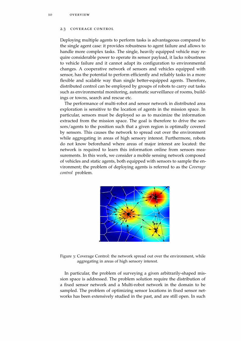
The performance of multi-robot and sensor network in distributed areaexploration is sensitive to the location of agents in the mission space. Inparticular, sensors must be deployed so as to maximize the informationextracted from the mission space. The goal is therefore to drive the sen-sors/agents to the position such that a given region is optimally coveredby sensors. This causes the network to spread out over the environmentwhile aggregating in areas of high sensory interest. Furthermore, robotsdo not know beforehand where areas of major interest are located: thenetwork is required to learn this information online from sensors mea-surements. In this work, we consider a mobile sensing network composedof vehicles and static agents, both equipped with sensors to sample the en-vironment; the problem of deploying agents is referred to as the Coveragecontrol problem.
Figure 3: Coverage Control: the network spread out over the environment, whileaggregating in areas of high sensory interest.
In particular, the problem of surveying a given arbitrarily-shaped mis-sion space is addressed. The problem solution require the distribution ofa fixed sensor network and a Multi-robot network in the domain to besampled. The problem of optimizing sensor locations in fixed sensor net-works has been extensively studied in the past, and are still open. In such
2.3 coverage control 11
problems, the solution is a Voronoi partition, where the optimal sensor do-main is a Voronoi cell in the partition and the optimal sensor location is acentroid of a Voronoi cell in the partition.
The approach proposed in this work is based on a distributed optimiza-tion that guide mobile agents towards points of maximum informative-ness. The method is then extended exploiting Voronoi tessellation in orderto keep track of the overall visited areas, this allows improvements in con-vergence time and in terms of overall knowledge.

Part II
T H E O R E T I C A L R E S U LT S
When sensors are deployed in unknown environments the mainissues arising regards locating the sensor in order to handlespatial goals, understanding best locations for agents in orderto gather more informative events, and designing locations fornew nodes in order to improve quality of services provided.These are referred as Localization, Beacon Placement, Cover-age Control issues for sensor and robot networks. The follow-ing chapters contain a comprehensive discussion regarding thistopics and solutions for above mentioned problems.


3L O C A L I Z AT I O N
Localization of mobile targets in structured environments is helped, ingeneral, by external elements that are called landmarks. Sensors are notperfect and an environmental model is never fully complete. Moreoverrobot’s wheels can slip, causing errors in odometry readings [2] and this letself-localization to be very unreliable. For these reasons, in order to operatein unknown environments, robotic agents must be capable to acquire andto use knowledge, to estimate insides of the setting and to answer in realtime for the situations that can occur.
3.1 objective and motivation
Localization may be defined as the problem of estimating the spatial rela-tionships among objects. In relative localization, dead-reckoning1 methods([23] and [7]) which consists of odometry and inertial navigation, are usedto calculate the robot position and orientation from a known initial pose.Odometry is a widely used localization method because of it is low cost,shows high updating rate, and is reasonably accurate when used in shortpath.
However its unbounded growth of time integration errors with the dis-tance traveled by the robot is unavoidable and represent a significant in-convenience [24]. Several approaches have been proposed to cope withodometric error propagation [46] and [44].
Conversely, absolute localization methods estimate the robot positionand orientation by detecting particular features of a known environment.This could be particular landmarks accurately located, or pre-existing pointsalready comprehended in the environment.Among the methods proposed in literature, geometric triangulation is oneof the most-widely used in the absolute localization thanks to the fact thatit provides a closed-form solution, to the accuracy of solutions providedand to its ability of determining both position and orientation of the tar-gets.The accuracy of triangulation algorithms depends upon both landmarksarrangement and the position of the mobile robot among them. Localiza-tion systems using some beacons have two advantages over localizationwith no beacons [27].Firstly, having beacons spatially distributed throughout the geographicalregion enables devices to compute their location in a scalable, decentral-
1 Dead-Reckoning is the process of calculating current position by using a previously de-termined position, and advancing that position based upon known or estimated speeds.Dead-Reckoning is a particular type of Odometry. A more detailed discussion about dead-reckoning is conduced in Section 6.1.1
15
16 localization
ized manner. Secondly, even when the application permits offline, central-ized position estimation algorithms, both the convergence and estimationaccuracy can be significantly improved by having some nodes as beacons[11]. Beacons constitute the underlying infrastructure of the localizationsystem.
3.1.1 Problem definition
This chapter presents a comprehensive solution to the problem of locatinga mobile target, usually a robot, in a planar mission space, given the loca-tion of three or more distinguishable landmarks in the environment, andmeasured angles between them as viewed from the robot.Locating, in this context, means determining robot’s location and orienta-tion uniquely. This situation arises when a mobile robot moves in a missionspace where other localization technologies (such as Global PositioningSystem (GPS)) are not available.
Aspects of triangulation to consider in order to achieve optimal resultsfor the robot pose2 in practical situation are:
1. the sensitivity analysis of the algorithm;
2. the optimal placement of landmarks;
3. the selection of some landmarks among the available ones to com-pute the robot pose;
4. the knowledge of the true landmark location in the world and thetrue location of the angular sensor on the robot.
Having a good sensor that provides precise angle measurements as wellas a good triangulation algorithm is not the only concern to get accuratepositioning results. Indeed, the angle sensor could be subject to non lin-earities in measuring angle range. Moreover the beacon locations are oftensubject to inaccuracies, which directly affect the positioning algorithm.
The main objective of this chapter is to present a three object triangu-lation algorithm, based on geometric triangulation, capable of working inthe entire mission space (except when beacons and robot are collinear) andfor any beacon ordering. Moreover the number of trigonometric computa-tion have to be minimized.
The second part of the chapter focuses on providing an accurate expres-sion for variance of the position estimated by the algorithm. This is anindispensable requisite that enables to give a statistical description to theestimated position, in order to perform statistical filtering.
The final part of this chapter deal with combining the estimated positionthrough geometric triangulation algorithm, with dead-reckoning data. Asit will be shown, this approach guarantees a high-rate, energy-saving androbust approach to the problem.
In particular Kalman filtering is used as it is a convenient way to fusetriangulation estimates together with odometry data.
2 pose indicates both the location and orientation of a robot
3.1 objective and motivation 17
3.1.2 Previous work
One of the first comprehensive work on localization has been carried outby Cohen and Koss. The work classifies the triangulation algorithms intofour groups: Geometric Triangulation, Iterative methods, Geometric circleintersection, Multiple beacon triangulation.
Several authors have noticed that the second type methods( Geometriccircle intersection) are the most popular in robotics [18] [35]. These methodscompute the intersection of the three circles passing through a couple ofbeacons and the robot.
Esteves et al. in [15] extend the algorithm presented by Cohen and Kossto work for any beacon ordering and to work outside the triangle formedby the three beacons. In [19] a method, working for every beacon ordering,is presented. The method divides the whole plane into seven region andhandles two specific configurations of the robot relatively to the beacons.
The most recent works [31] [39] propose novel methods to achieve asolution to the geometric triangulation relying on the idea of using theradical axis of circles. The methods still works in the entire plane naively.Furthermore it only uses basic arithmetic computations and two cot(·)computation, leading to a drastic reduction in computational complexity.
This work aims at improving performances of triangulation algorithmsby combining the position estimates with odometry data. Similar approaches,based on EKF, have already been proposed in previous works as in [17] and[16] but in these cases the filtering was used on the measures of angles be-tween the robot and the beacons.
3.1.3 Contribution
In the first part of the chapter, arising from [39] we report a comprehen-sive description of ToTal algorithm proposed by Pierlot and Van Droogen-broeck. Particular attention is paid both to computational reduction broughtwith respect to previous works and to improvements in the robustness ofthe solution, introduced thanks to the exploitation of radical axes of circlesemployed.
In the second part of the chapter, a novel method capable of combiningtriangulation solution together with odometry is proposed.
We underline that more appreciated approaches in published works in-tegrate a prediction phase, based on the odometric data and the robot kine-matics, and a correction -or estimation- phase that takes into account ex-ternal measurements. The approach used in this work is based on Kalmanfiltering [48]. In fact, Kalman filtering results as a suitable way to combinedata arising from internal kinematic model together with triangulationdata.
The chapter is completed with an overview on kinematic models forWheeled Mobile Robots and Quadrotors.
18 localization
3.2 navigation systems : methods classification
Landmark-based navigation of autonomous mobile robots or vehicles hasbeen widely adopted in industry. In general, the methods for locating mo-bile robots in the real world are divided into two categories:
1. Relative positioning;
2. Absolute positioning.
In relative positioning, odometry (in particular dead-reckoning) and iner-tial navigation are commonly used to calculate the robot positions froma start reference point at a high updating rate. Odometry is one of themost popular techniques based on internal sensors for position estimationbecause of its ease of use in real time. However, a compromising disad-vantage affects this method: it suffers of an unbounded accumulation oferrors due to inaccuracies of sensors. Therefore, frequent corrections to theestimated position become necessary.
In contrast, absolute positioning relies on detecting and recognizing dif-ferent features in the environment, in order for a mobile robot to reach adestination and implement a specified task. These environment featuresare normally divided into two types:
1. Natural landmarks;
2. Artificial landmarks.
Among these, natural landmark navigation is flexible as no explicit artifi-cial landmarks are needed, however it may not work well when landmarksare sparse and often the environment must be a priori known. Althoughthe artificial landmark and active beacon approaches are less flexible, theability in finding landmarks is enhanced and the process of map buildingis simplified.
To make the use of mobile robots in daily deployment feasible, it isnecessary to reach a trade-off between costs and benefits. Often, this dis-courages the use of expensive sensors such as vision systems and GPS infavor of cheaper sensing devices, for example laser or encoders, and callsfor efficient algorithms that can guarantee real-time performance in thepresence of insufficient or conflicting data.
Two scenarios could be hypothesized regarding nodes’ behavior:
1. Anchor-based, in which only landmark (or anchor) nodes know theirabsolute position, while robotic nodes exploit landmarks to deter-mine their absolute position;
2. Anchor-free, in which any node does not know its absolute location,in this case a relative coordinate reference is used.
The first type of methods enables to know the absolute location of nodesin an unique way, but this requires anchor nodes to know their absolute lo-cation (using for example GPS systems) and these should be quite densely
3.2 navigation systems : methods classification 19
allocated in the configuration space, as they can not move. The secondtype of methods enable a more flexible arrangement of anchor, so nodescould be placed in a random way. Although anchor-free systems enablemore flexibility in the deployment phase, the absence of anchor nodes pro-duce an unbounded error propagation in the network.Both in anchor-based and in anchor-free systems, the position computa-tion is performed basing on the knowledge of relative distances (or an-gles) between nodes. Three types of techniques could be used to computerelative distance of a node with neighbors:
1. Range based;
2. Angle based;
3. Range free.
Range-based techniques make use of Euclidean distances, in fact nodesare equipped with sensors to estimate relative distances with neighbornodes. Algorithm such as Min-Max, Trilateration and Multilateration be-long to this family of methods [8] .
Angle-based techniques are based on angular distances between nodes,in fact robots are equipped with sensors capable of estimating relative an-gles with neighbor nodes. This type of techniques exploit geometric andtrigonometric properties as motivated in [8]. Geometrical triangulation be-long to this family of methods.
Range-free techniques are based on virtual coordinate references, andfor this reason, they are independent from Euclidean distances.A range-free method requires no distances or angles measurement amongnodes, so they do not require additional hardware; and instead use prop-erties of the wireless sensor network to obtain location information.
estimating relative distances for range-based techniques
The estimation of relative distances between nodes is usually referredas Ranging technique. There are three main types of ranging techniques:
• Time of Arrival (ToA);
• Time Difference of Arrival (TDoA);
• Received Signal Strength (RSS).
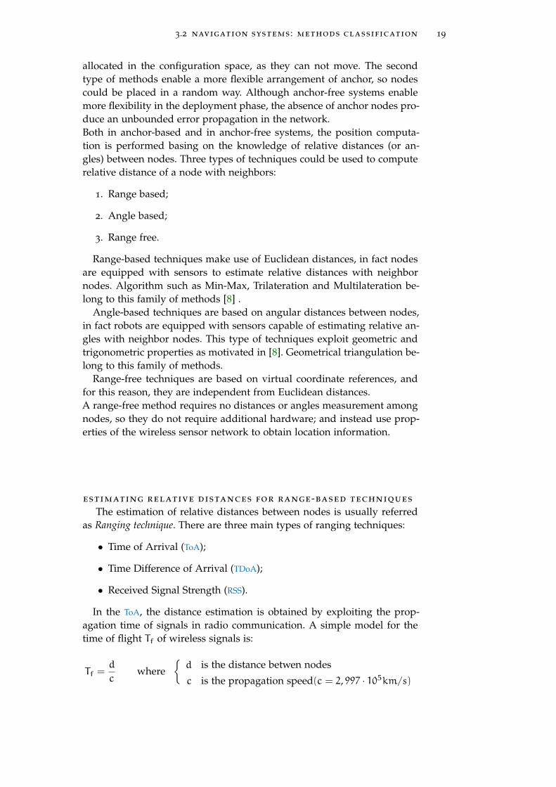
In the ToA, the distance estimation is obtained by exploiting the prop-agation time of signals in radio communication. A simple model for thetime of flight Tf of wireless signals is:
Tf =d
cwhere
d is the distance betwen nodes
c is the propagation speed(c = 2, 997 · 105km/s)

20 localization
Two methods can be used: One-way ToA, and Two-way ToA.
Figure 4: One-way ToA.
In one-way ToA, node A sends sig-nal at time t1, the signal arrives toB at time t2. In this way node Bis able to estimate the relative dis-tance just exploiting:Tf = t2 − t1
Figure 5: Two-way ToA.
In two-way ToA, node A sendssignal at time t1 and the same ar-rives to node B at time t2. NodeB computes the message in tdtime and then sends a responseto node A at time t3. The samearrives at A at time t4. The timeof flight is then calculated us-ing:Tf =
(t2−t1)+(t4−t3)2 .
Figure 6: TDoA.
In the TDoA technique, an estima-tion for the speed of propagation isperformed in order to avoid errorslinked to obstacles in unknown en-vironments.In particular, node A transmits twotypes of signals: RF (Radio Fre-quency signal) and US (UltrasoundPulse signal), traveling at differentspeeds. A graphical explanation ofsignals sent is shown in the fig-ure on the right. Receiver then esti-mates relative distances by exploit-ing the difference of times of ar-rival of the two signals.
RSS techniques are based on power attenuation during the propagationof a transmitted signal. Every receiver is thus able to estimate relative dis-tances by evaluating the strength of the signal received. The estimate of
3.2 navigation systems : methods classification 21
a received signal (in dBm) is performed by the Received Signal StrengthIndicator (RSSI). The main advantage of this method is that it does not re-quire additional hardware, however it guarantees less precision than previ-ous presented techniques. In fact, signals could be reflected, absorbed andattenuated by obstacles. This is mainly used in application where energyconsumption is very relevant and no further hardware can be mounted onagents. In particular, the distance from the transmitter could be evaluatedexploiting Friis equation:
PR = PTGTGRλ
2
(4π)2dn
where:
• PR, PT : power of received and transmitted signals [Watt];
• GR, GT : receiver and transmitter antennae gain [ ];
• λ = cf : wavelength [m];
• d: distance [m];
• n: signal propagation constant.
estimating relative angles for angle-based techniques
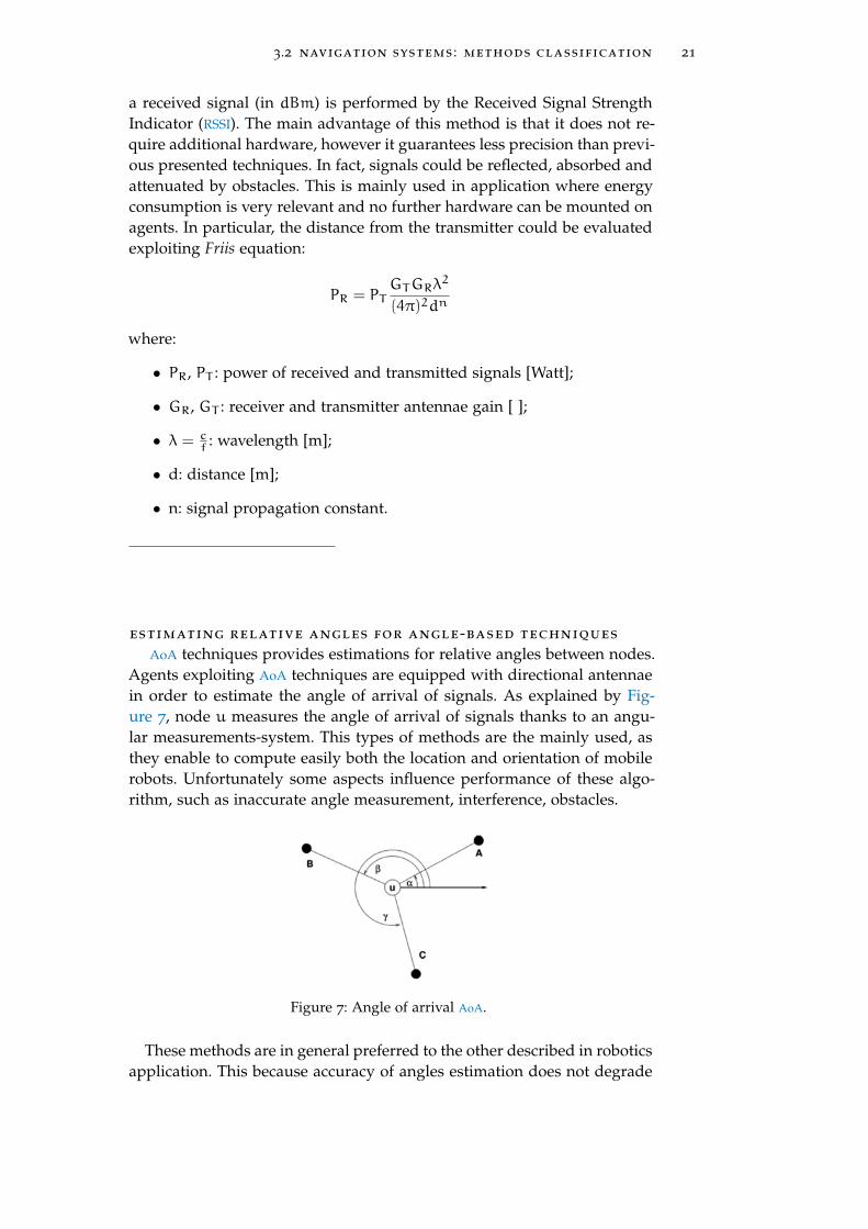
AoA techniques provides estimations for relative angles between nodes.Agents exploiting AoA techniques are equipped with directional antennaein order to estimate the angle of arrival of signals. As explained by Fig-ure 7, node u measures the angle of arrival of signals thanks to an angu-lar measurements-system. This types of methods are the mainly used, asthey enable to compute easily both the location and orientation of mobilerobots. Unfortunately some aspects influence performance of these algo-rithm, such as inaccurate angle measurement, interference, obstacles.
Figure 7: Angle of arrival AoA.
These methods are in general preferred to the other described in roboticsapplication. This because accuracy of angles estimation does not degrade
22 localization
with the increasing of distances between beacons and the target. In fact,this method results as one of the most reliable as accuracy of angles esti-mation depends only on the presence or absence of obstacles in the fieldof view.
3.2.1 Methods overview
One of the first comprehensive reviewing work has been carried out byCohen and Koss [8]. In their paper, triangulation algorithms have beenclassified into four groups:
1. Geometric Triangulation;
2. Geometric Circle Intersection;
3. Iterative Methods (Iterative Search, Newton-Raphson, etc.);
4. Multiple Beacons Triangulation.
The first group makes an intensive use of trigonometric functions andexploits relative angles between landmarks as viewed from the robot. Thesolution can be computed in a closed form. The calculus is based on thegeometry of the locations of landmarks and the location of the robot. Prim-itive types of these algorithms required properly ordered landmarks.
Algorithms of the second group determine parameters (radius and cen-ter) of the two circles passing through a couple of beacons and the robot.The robot position is then deduced by computing the intersection betweenthese two circles and exploiting angles measured by the robot. This type isthe most popular for solving the three object triangulation problem. Manyvariations and improvements have been proposed [35] [34] in order to re-duce limitations of the original method such as working for any beaconordering and to work outside the triangle formed by the three beacons.
The third group linearizes the trigonometric relations to converge tothe robot position after some iterations, exploiting the Newton-Raphsonmethod [50].
Iterative methods, based principally on Iterative search algorithm, whichconsists in searching the robot position through the possible space of ori-entation, and by using a closeness measure of the solution. The fourthgroup addresses the more general problem of finding the robot pose frommore than three angle measurements, which is a overdetemined problem.This solution is preferable in presence of massive measurement noise insensors.
In general, if the setup contains three beacons only, or if the robot haslimited on-board processing capabilities, Geometric Triangulation and Geo-metric circle intersection are the best candidates. Iterative methods and Mul-tiple Beacons Triangulation are appropriate if the application must handle
3.3 triangulation 23
multiple beacons and if it can accommodate a higher computational cost.The main drawback of Iterative methods is the convergence issue, whileMultiple Beacons Triangulation has the disadvantage of high computationalcosts. The drawback of the first and second group are usually a lack ofprecision related to: the consistency of the methods when the robot is lo-cated outside the triangle defined by the three beacons, the strategy tofollow when falling into some particular geometrical cases, the reliabilitymeasure of the computed position. Simple methods of the first and secondgroups usually fail to propose a proper answer to all these concerns.
Therefore, the focus of this thesis is on the use of a specific hardwarefor localization based on AoA (radio, laser scanner etc.) and artificial land-marks for the position estimation of a mobile robot. Geometric triangula-tion is therefore the method preferred for the reasons just explained.
3.3 triangulation
It is difficult to compare all the above mentioned methods, because theyoperate in different conditions and have distinct behavior. In practice, thechoice is dictated by the application requirements, and some compromises.
Thanks to the availability and accuracy of angle measurements systems,geometric triangulation has emerged as a widely used, robust, accurate,and flexible technique [15]. Furthermore, in geometric triangulation therobot can compute its orientation in addition to its position, so that thecomplete pose of the robot can be found. This feature is proper of geomet-ric triangulation methods, and in general alternative methods presenteddo not guarantee this behavior. For the reasons presented, triangulationmethods are the more suitable for the assumptions done in this work.
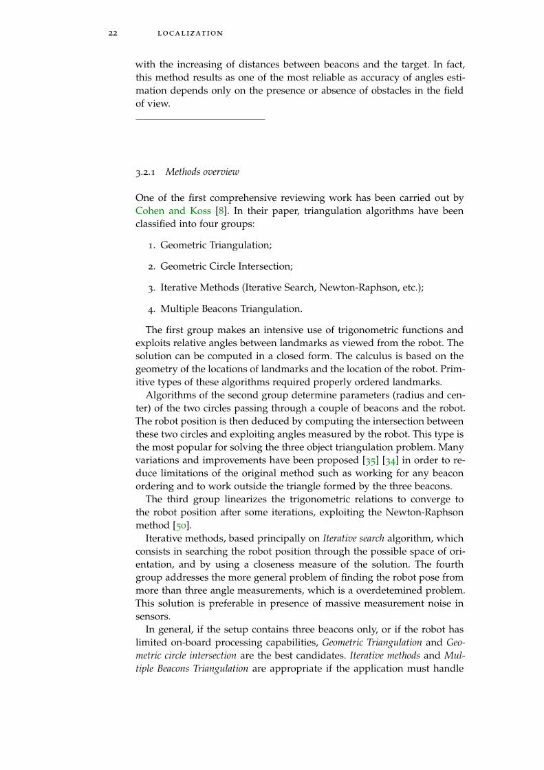
Figure 8 illustrates a typical triangulation setup. Here the problem isreferred to a 2-D plane. Angles φ1, φ2 and φ3 may be used by a trian-gulation algorithm in order to compute the robot position (xR,yR) andorientation θ.
Figure 8: Triangulation setup in the 2-D plane. R denotes the robot, B1, B2 andB3 are the beacons. φ1, φ2 and φ3 are the angles for beacons, measuredrelatively from the robot orientation frame.
24 localization
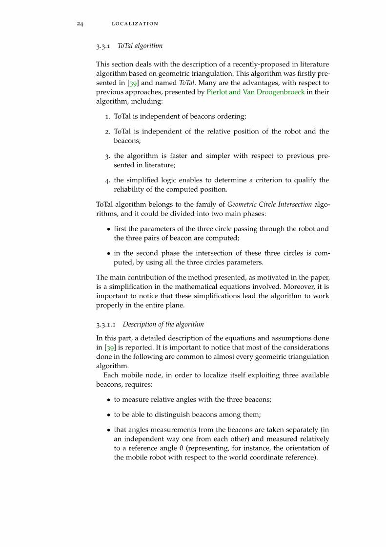
3.3.1 ToTal algorithm
This section deals with the description of a recently-proposed in literaturealgorithm based on geometric triangulation. This algorithm was firstly pre-sented in [39] and named ToTal. Many are the advantages, with respect toprevious approaches, presented by Pierlot and Van Droogenbroeck in theiralgorithm, including:
1. ToTal is independent of beacons ordering;
2. ToTal is independent of the relative position of the robot and thebeacons;
3. the algorithm is faster and simpler with respect to previous pre-sented in literature;
4. the simplified logic enables to determine a criterion to qualify thereliability of the computed position.
ToTal algorithm belongs to the family of Geometric Circle Intersection algo-rithms, and it could be divided into two main phases:
• first the parameters of the three circle passing through the robot andthe three pairs of beacon are computed;
• in the second phase the intersection of these three circles is com-puted, by using all the three circles parameters.
The main contribution of the method presented, as motivated in the paper,is a simplification in the mathematical equations involved. Moreover, it isimportant to notice that these simplifications lead the algorithm to workproperly in the entire plane.
3.3.1.1 Description of the algorithm
In this part, a detailed description of the equations and assumptions donein [39] is reported. It is important to notice that most of the considerationsdone in the following are common to almost every geometric triangulationalgorithm.
Each mobile node, in order to localize itself exploiting three availablebeacons, requires:
• to measure relative angles with the three beacons;
• to be able to distinguish beacons among them;
• that angles measurements from the beacons are taken separately (inan independent way one from each other) and measured relativelyto a reference angle θ (representing, for instance, the orientation ofthe mobile robot with respect to the world coordinate reference).
3.3 triangulation 25
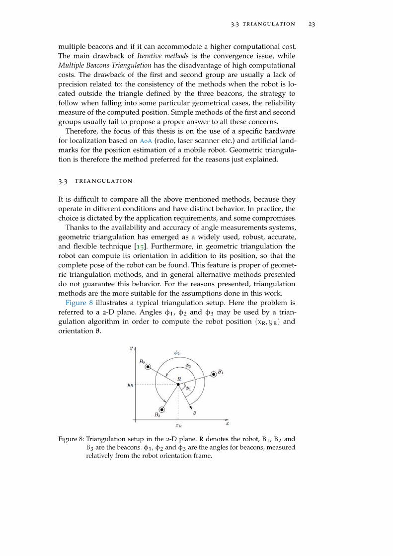
We start by determining the locus of the robot position R, that see twofixed beacons, B1 and B2.
Figure 9: Locus of robot positions given the angle between beacons as seen fromthe robot.
Proposition 3.3.1 (Locus of robot positions). Given the angle between B1 andB2 as seen from the robot, φ12, the locus of possible robot positions is an arc ofthe circle passing through B1, B2 and R.
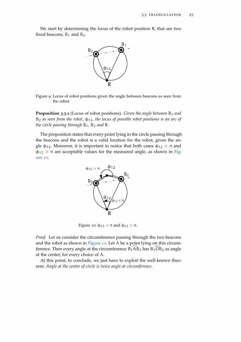
The proposition states that every point lying in the circle passing throughthe beacons and the robot is a valid location for the robot, given the an-gle φ12. Moreover, it is important to notice that both cases φ12 < π andφ12 > π are acceptable values for the measured angle, as shown in Fig-ure 10.
Figure 10: φ12 < π and φ12 > π.
Proof. Let us consider the circumference passing through the two beaconsand the robot as shown in Figure 11. Let A be a point lying on this circum-ference. Then every angle at the circumference B1AB2 has B1OB2 as angleat the center, for every choice of A.
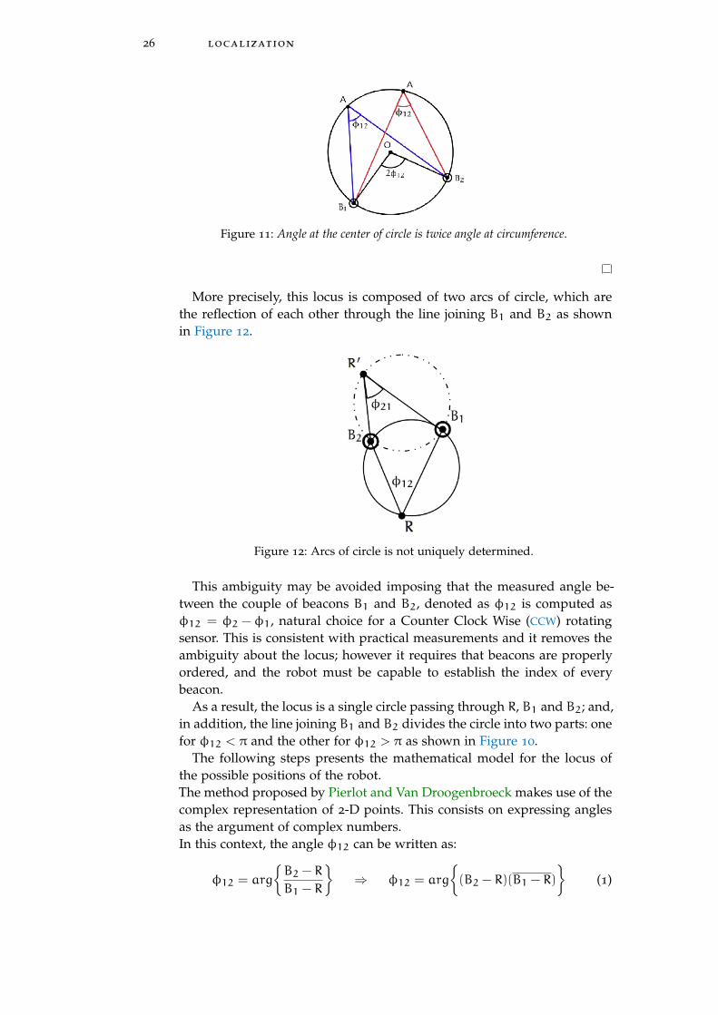
At this point, to conclude, we just have to exploit the well-known theo-rem: Angle at the center of circle is twice angle at circumference.
26 localization
Figure 11: Angle at the center of circle is twice angle at circumference.
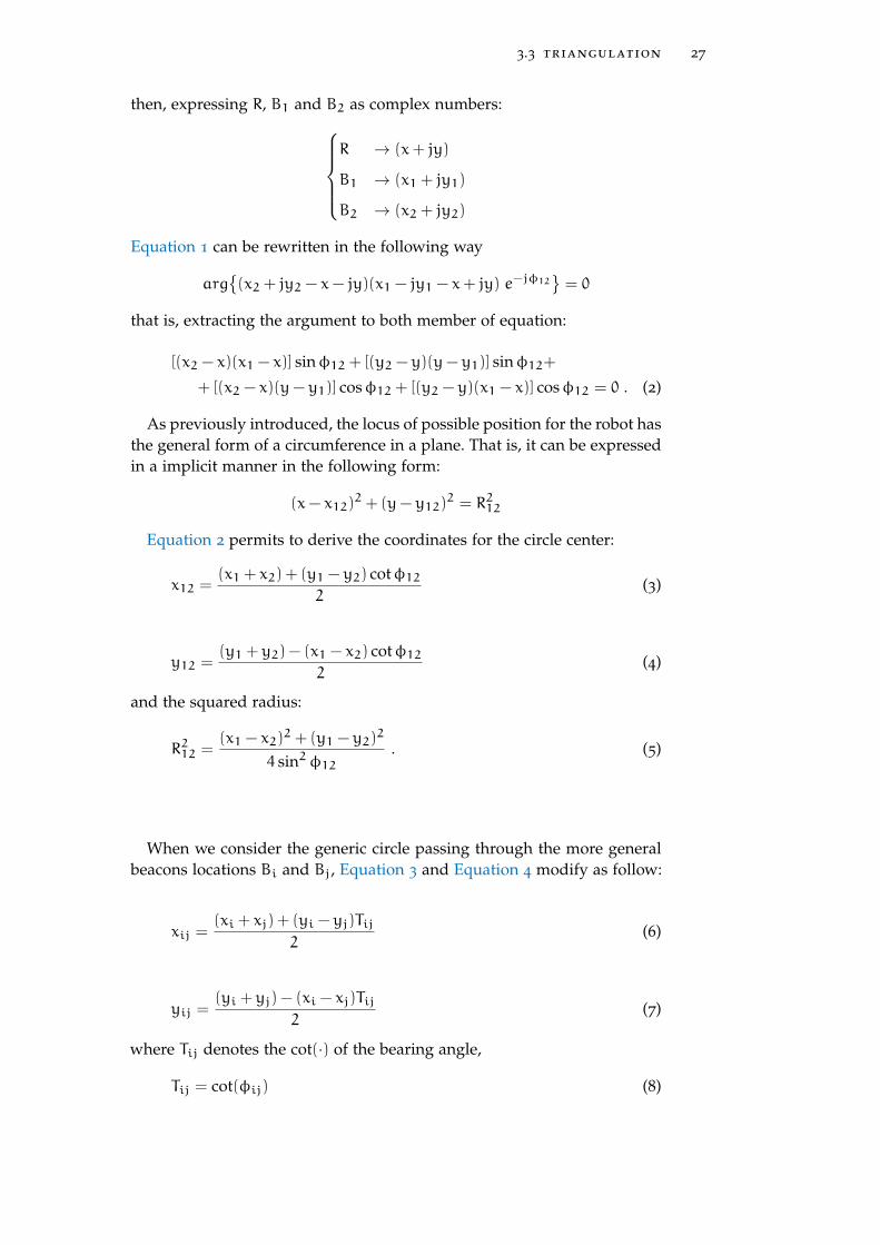
More precisely, this locus is composed of two arcs of circle, which arethe reflection of each other through the line joining B1 and B2 as shownin Figure 12.
Figure 12: Arcs of circle is not uniquely determined.
This ambiguity may be avoided imposing that the measured angle be-tween the couple of beacons B1 and B2, denoted as φ12 is computed asφ12 = φ2 − φ1, natural choice for a Counter Clock Wise (CCW) rotatingsensor. This is consistent with practical measurements and it removes theambiguity about the locus; however it requires that beacons are properlyordered, and the robot must be capable to establish the index of everybeacon.
As a result, the locus is a single circle passing through R, B1 and B2; and,in addition, the line joining B1 and B2 divides the circle into two parts: onefor φ12 < π and the other for φ12 > π as shown in Figure 10.
The following steps presents the mathematical model for the locus ofthe possible positions of the robot.The method proposed by Pierlot and Van Droogenbroeck makes use of thecomplex representation of 2-D points. This consists on expressing anglesas the argument of complex numbers.In this context, the angle φ12 can be written as:
φ12 = arg
B2 − R
B1 − R
⇒ φ12 = arg
(B2 − R)(B1 − R)
(1)
3.3 triangulation 27
then, expressing R, B1 and B2 as complex numbers:R → (x+ jy)
B1 → (x1 + jy1)
B2 → (x2 + jy2)
Equation 1 can be rewritten in the following way
arg(x2 + jy2 − x− jy)(x1 − jy1 − x+ jy) e
−jφ12= 0
that is, extracting the argument to both member of equation:
[(x2 − x)(x1 − x)] sinφ12 + [(y2 − y)(y− y1)] sinφ12+
+ [(x2 − x)(y− y1)] cosφ12 + [(y2 − y)(x1 − x)] cosφ12 = 0 . (2)
As previously introduced, the locus of possible position for the robot hasthe general form of a circumference in a plane. That is, it can be expressedin a implicit manner in the following form:
(x− x12)2 + (y− y12)
2 = R212
Equation 2 permits to derive the coordinates for the circle center:
x12 =(x1 + x2) + (y1 − y2) cotφ12
2(3)
y12 =(y1 + y2) − (x1 − x2) cotφ12
2(4)
and the squared radius:
R212 =(x1 − x2)
2 + (y1 − y2)2
4 sin2φ12. (5)
When we consider the generic circle passing through the more generalbeacons locations Bi and Bj, Equation 3 and Equation 4 modify as follow:
xij =(xi + xj) + (yi − yj)Tij
2(6)
yij =(yi + yj) − (xi − xj)Tij
2(7)
where Tij denotes the cot(·) of the bearing angle,
Tij = cot(φij) (8)
28 localization
Equation 5 becomes
Rij =(xi − xj)
2 + (yi − yj)2
4 sin2φij. (9)
Equations (6), (7) cij and (9) completely describe the circle Cij with centercij of coordinates (xij,yij).
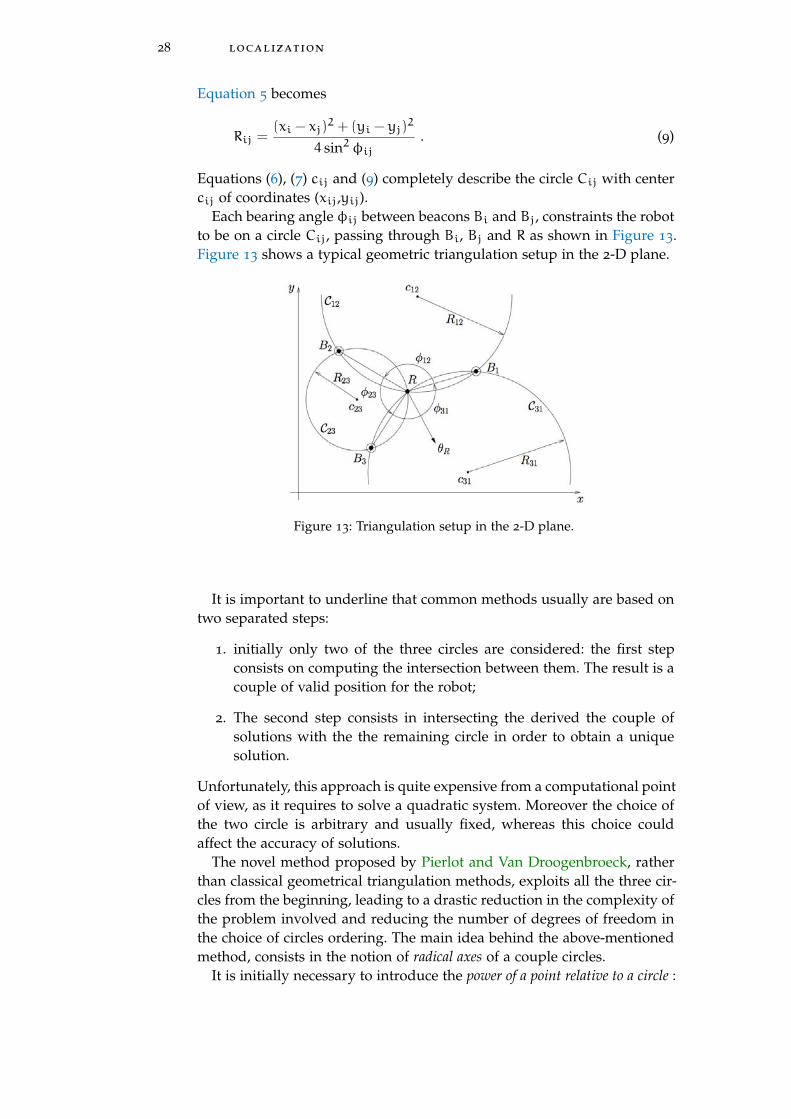
Each bearing angle φij between beacons Bi and Bj, constraints the robotto be on a circle Cij, passing through Bi, Bj and R as shown in Figure 13.Figure 13 shows a typical geometric triangulation setup in the 2-D plane.
Figure 13: Triangulation setup in the 2-D plane.
It is important to underline that common methods usually are based ontwo separated steps:
1. initially only two of the three circles are considered: the first stepconsists on computing the intersection between them. The result is acouple of valid position for the robot;
2. The second step consists in intersecting the derived the couple ofsolutions with the the remaining circle in order to obtain a uniquesolution.
Unfortunately, this approach is quite expensive from a computational pointof view, as it requires to solve a quadratic system. Moreover the choice ofthe two circle is arbitrary and usually fixed, whereas this choice couldaffect the accuracy of solutions.
The novel method proposed by Pierlot and Van Droogenbroeck, ratherthan classical geometrical triangulation methods, exploits all the three cir-cles from the beginning, leading to a drastic reduction in the complexity ofthe problem involved and reducing the number of degrees of freedom inthe choice of circles ordering. The main idea behind the above-mentionedmethod, consists in the notion of radical axes of a couple circles.
It is initially necessary to introduce the power of a point relative to a circle :

3.3 triangulation 29
Definition 3.1. The power of a point p relative to a circle C, is defined by:
PC,p = (x− xc)2 + (y− yc)
2 − R2
When the circles involved are two, the definition can be extended toradical axes of a couple of circles:
Definition 3.2. The radical axis of a couple of circles C1 and C2 is the locusof points having the same power with respect to both circles.
Example 3.3.1. Given a couple of circles, possible configurations are twofold:
Figure 14: Radical axis of a couple of circles.
When three circles are considered, radical axes concerning every coupleof them, intersect in a single point, as shown in Figure 15.
Figure 15: Radical axes concerning three circles. Possible arrangements are three.Red points represent intersections between radical axes.
It is important to underline that their intersection point is the uniquepoint of the plane having the same power with respect to every singlecircle.
30 localization
The example motivates the following:
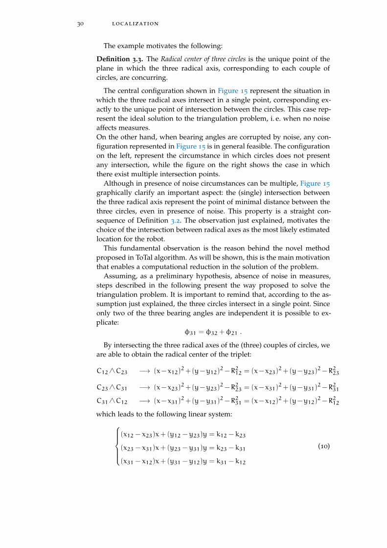
Definition 3.3. The Radical center of three circles is the unique point of theplane in which the three radical axis, corresponding to each couple ofcircles, are concurring.
The central configuration shown in Figure 15 represent the situation inwhich the three radical axes intersect in a single point, corresponding ex-actly to the unique point of intersection between the circles. This case rep-resent the ideal solution to the triangulation problem, i. e. when no noiseaffects measures.On the other hand, when bearing angles are corrupted by noise, any con-figuration represented in Figure 15 is in general feasible. The configurationon the left, represent the circumstance in which circles does not presentany intersection, while the figure on the right shows the case in whichthere exist multiple intersection points.
Although in presence of noise circumstances can be multiple, Figure 15
graphically clarify an important aspect: the (single) intersection betweenthe three radical axis represent the point of minimal distance between thethree circles, even in presence of noise. This property is a straight con-sequence of Definition 3.2. The observation just explained, motivates thechoice of the intersection between radical axes as the most likely estimatedlocation for the robot.
This fundamental observation is the reason behind the novel methodproposed in ToTal algorithm. As will be shown, this is the main motivationthat enables a computational reduction in the solution of the problem.
Assuming, as a preliminary hypothesis, absence of noise in measures,steps described in the following present the way proposed to solve thetriangulation problem. It is important to remind that, according to the as-sumption just explained, the three circles intersect in a single point. Sinceonly two of the three bearing angles are independent it is possible to ex-plicate:
φ31 = φ32 +φ21 .
By intersecting the three radical axes of the (three) couples of circles, weare able to obtain the radical center of the triplet:
C12∧C23 −→ (x−x12)2+(y−y12)
2−R212 = (x−x23)2+(y−y23)
2−R223
C23∧C31 −→ (x−x23)2+(y−y23)
2−R223 = (x−x31)2+(y−y31)
2−R231
C31∧C12 −→ (x−x31)2+(y−y31)
2−R231 = (x−x12)2+(y−y12)
2−R212
which leads to the following linear system:(x12 − x23)x+ (y12 − y23)y = k12 − k23
(x23 − x31)x+ (y23 − y31)y = k23 − k31
(x31 − x12)x+ (y31 − y12)y = k31 − k12
(10)
3.3 triangulation 31
where the new introduced quantity kij is defined as follows:
kij =x2ij + y
2ij − R
2ij
2. (11)
As a result, the solution to the geometrical triangulation problem pre-sented - that was initially described as a geometrical and trigonometricalissue - has been re-conduced to the solution of a three linear equation-system. The coordinates of the power center, that is, the estimated robotposition can then be obtained as the solution of the following linear sys-tem:
Ax = b . (12)
It is important to underline two important characteristics for the prob-lem:
1. the linear system (12) consists of three equations and two unknowns;
2. any equation that appears in Equation 12 can be obtained as additionof the others.
It is important to notice that 2. mathematically proves that the threeradical axis concur in an unique point, as previously introduced.
Linear system (12) can be expressed in matrix form, according to (12),in the following manner:
A =
[x12 − x23 y12 − y23
x23 − x31 y23 − y31
], b =
[k12 − k23
k23 − k31
]The computation of the solution through (xR,yR) = A−1b, leads to:
xR =(k12 − k23)(y23 − y31) − (y12 − y23)(k23 − k31)
det(A)(13)
yR =(x12 − x23)(k23 − k31) − (k12 − k23)(x23 − x31)
det(A)(14)
where we have used:
det(A) = (x12 − x23)(y23 − y31) − (y12 − y23)(x23 − x31)
Therefore, Equation 13 and Equation 14 are the mathematical expres-sions that enable to compute actual position of the robot, when exploitingfollowing data:
• the three circles centers coordinates (xij,yij) ∀ i = 1, 2, 3 , j =
1, 2, 3 i 6= j;
• the three beacons locations (xi,yi) ∀ i = 1, 2, 3 ;
• the three bearing angles in order to compute Tij = cot(φij) ∀ i =1, 2, 3 , j = 1, 2, 3 i 6= j .
32 localization
3.3.2 Final version of ToTal algorithm and discussion
It is possible to further simplify equations presented in order to producean improved version for the algorithm.First of all it is possible to replace expression Equation 9 for R2ij in Equa-tion 11, for kij, obtaining after some simplifications:
kij =xixk + yiyj + Tij(xjyi − xiyj)
2.
In addition, a further simplification (often used in many triangulation al-gorithm) consists in translating coordinates in such a way to locate theorigin of the reference frame in the location of an arbitrarily-chosen bea-con.In this case, we arbitrarily choose B2 as the origin, so other beacons coor-dinates become:
B ′1 = B1 −B2 = x1 − x2,y1 − y2
B ′2 = B2 = 0, 0
B ′3 = B3 −B2 = x3 − x2,y3 − y2
(15)
Then, noticing that the factor 12 involved in (6) and (7), as well as in (11),for kij, cancels when used in robot position parameters, we can introducemodified circle center coordinates:
x ′ij = 2xij,
y ′ij = 2yij,
and modified parameter kij:
k ′ij = 2kij .
Therefore, robot position (xR,yR) can be computed exploiting:
xR = x2 +k ′31(y
′12 − y
′23)
det(A)(16)
yR = y2 +k ′31(x23 − x12)
det(A)(17)
a complete treatment of mathematical steps and a detailed description ofequations involved can be found in [39].
Observation 1. There are two particular cases that require special treatment:
• infinite values of cot(·) function, in (8);
• cases in which det(A) = 0, in (13) and (14) that lead to invalid robotestimated position.
3.3 triangulation 33
When a bearing angle φij is equal to 0 or π, then the cot(·) functionassumes non-finite values. This is the case when the robot to be localizedstands on the line joining a couple f beacons Bi and Bj.
Typical solutions very often exploited in literature consist on limitingthe cot(·) value to a minimum or maximum value, corresponding to asmall angle that is far below the measurement precision. Typical valuesare ±108, which corresponds to an angle of about ±10−8rad.
More accurate solutions to some of these peculiar cases can be foundin literature. For example, Pierlot and Van Droogenbroeck in [39] proposesome adjustments in the algorithms, when one of the two angles measuredis equal to 0 or π, which makes the method reliable.
However, it is important to underline that in such cases in which beaconsand the robot are collinear, geometric triangulation is unable to find anysolution to the problem as not enough parameters are available. In fact,this is the case in when the solution computed as intersection of the threecircles is not a single point, but a locus. This problem is common to allgeometric triangulation-based methods, nevertheless several solutions canbe exploited as motivated in Observation 1.
In addition orientation of the robot θR may be determined by using bea-cons locations Bi and its corresponding angle φi, once the robot positionis known, by exploiting:
θR = atan2(yi − yR, xi − xR) −φi (18)
where atan2(x,y) denotes the argument arg(x + jy) of the complexnumber x+ jy.
Finally, it is important to underline that:
1. each localization iteration requires each mobile agent to transmit toevery sensing beacon (at least three) a request;
2. each beacon sends a response containing its own position;
3. angles of arrival measurements are then taken by mobile agent;
4. the mobile robot is then able to perform geometric triangulation;
then each triangulation application requires the transmission of (at least)three data packet, the reception of as much packets, and an angle of arrivalmeasurement.
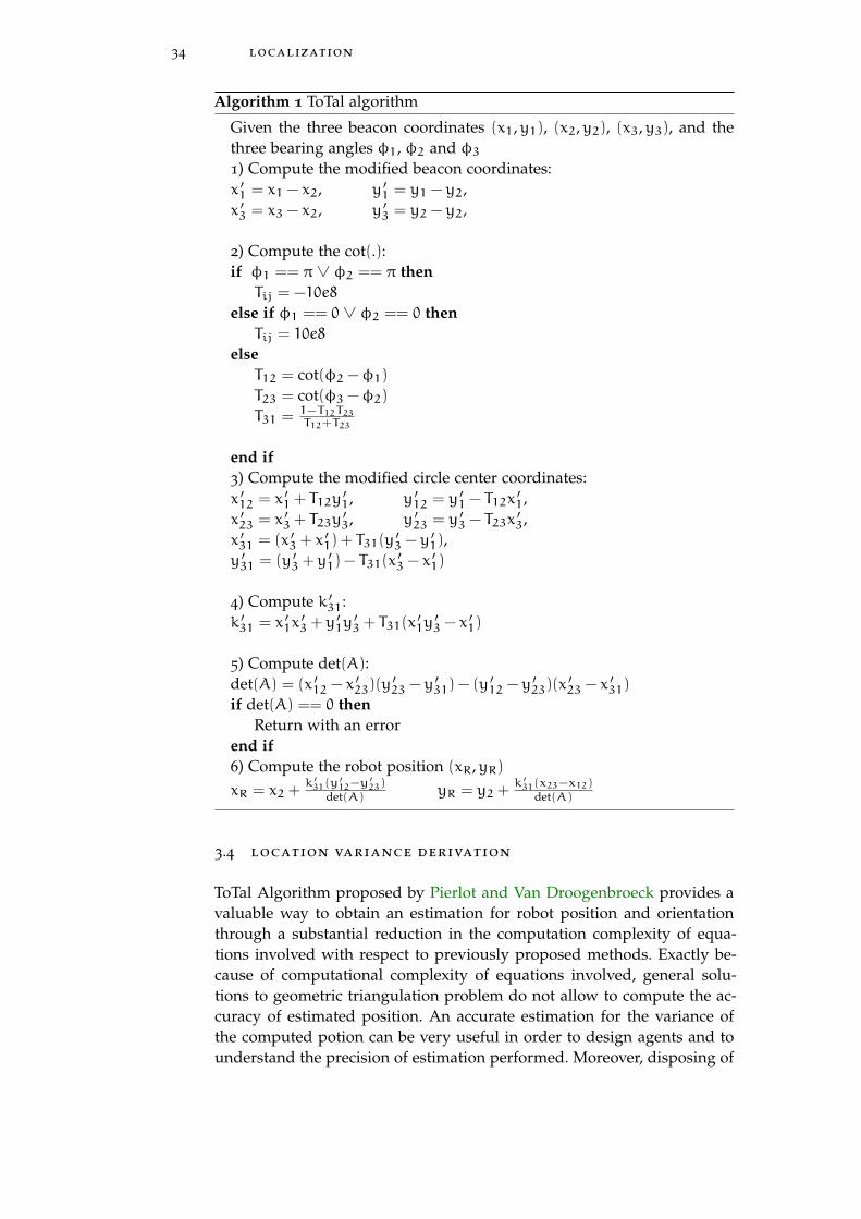
Algorithm 1 proposes a detailed description for the algorithm in pseudo-code.
34 localization
Algorithm 1 ToTal algorithm
Given the three beacon coordinates (x1,y1), (x2,y2), (x3,y3), and thethree bearing angles φ1, φ2 and φ31) Compute the modified beacon coordinates:x ′1 = x1 − x2, y ′1 = y1 − y2,x ′3 = x3 − x2, y ′3 = y2 − y2,
2) Compute the cot(.):if φ1 == π ∨ φ2 == π thenTij = −10e8
else if φ1 == 0 ∨ φ2 == 0 thenTij = 10e8
elseT12 = cot(φ2 −φ1)T23 = cot(φ3 −φ2)T31 =
1−T12T23T12+T23
end if3) Compute the modified circle center coordinates:x ′12 = x
′1 + T12y
′1, y ′12 = y
′1 − T12x
′1,
x ′23 = x′3 + T23y
′3, y ′23 = y
′3 − T23x
′3,
x ′31 = (x ′3 + x′1) + T31(y
′3 − y
′1),
y ′31 = (y ′3 + y′1) − T31(x
′3 − x
′1)
4) Compute k ′31:k ′31 = x
′1x′3 + y
′1y′3 + T31(x
′1y′3 − x
′1)
5) Compute det(A):det(A) = (x ′12 − x
′23)(y
′23 − y
′31) − (y ′12 − y
′23)(x
′23 − x
′31)
if det(A) == 0 thenReturn with an error
end if6) Compute the robot position (xR,yR)xR = x2 +
k ′31(y′12−y
′23)
det(A) yR = y2 +k ′31(x23−x12)
det(A)
3.4 location variance derivation
ToTal Algorithm proposed by Pierlot and Van Droogenbroeck provides avaluable way to obtain an estimation for robot position and orientationthrough a substantial reduction in the computation complexity of equa-tions involved with respect to previously proposed methods. Exactly be-cause of computational complexity of equations involved, general solu-tions to geometric triangulation problem do not allow to compute the ac-curacy of estimated position. An accurate estimation for the variance ofthe computed potion can be very useful in order to design agents and tounderstand the precision of estimation performed. Moreover, disposing of

3.4 location variance derivation 35
location uncertain, as a function of beacons positions uncertain and anglesof arrival uncertain, permits to create a statistical description for the modelinvolved and to enforce statistical filtering to noisy measurements.
In [39] a sensitivity analysis of the computed position with respect toangles of arrival φ1, φ2 and φ3 is performed. Although this leads an un-certain analysis of the computed position as function of the (non-linear)angles of arrival, it does not permit to take into account uncertain linkedto non-exact positions of beacons.
The purpose of this work is to derive a detailed, closed-form expressionfor variance of computed position as a function of beacons locations uncer-tain and of angles of arrival uncertain. In order to accomplish this task, thepropagation of uncertainty law has been exploited. Since functions involvedin geometric triangulation are trigonometric, i. e. non-linear, they have tobe linearized by approximation to a first-order Taylor series expansion.
Example 3.4.1. In general contexts, given the non-linear function:
f(x) : Rn → Rm,
the Taylor expansion would be, assuming that x is concentrated around itsmean M(x):
f(x) ' f(M(x)) +
[∂f(x)
∂x
]M(x)
(x−M(x)) .
Since f(M(x)) is constant as function of x, it does not contribute to theerror in f. Therefore, the covariance propagation follows the linear rule:
Covf(x) =
[∂f(x)
∂x
]Covx
[∂f(x)
∂x
]T= J ·Covx · JT , (19)
where J indicates the Jacobian matrix of f(x):
J =∂f(x)
∂x
and Covx is the covariance matrix of vector x.
The derivation of a closed-form expression for uncertain, proposed inthis work, makes use of geometric properties of circles employed in thethree object triangulation problem. In the following we motivate our choiceof exploiting the uncertain in the three circles areas to compute uncertainon estimated robot position.
Figure 16 presents a simple case in which we deal with uncertainty inthe knowledge about position of one of the three beacons employed B1.The yellow circle represents uncertain on location for node B1, while it islocated exactly in the mean value of its distribution, identified by blackan white dot patterns. It is important to notice that this type of uncertain

36 localization
could be associated to both uncertain on the actual position of the node,and to the uncertain on the measured angle performed by the robot.
Assuming that actual position of the beacon can be modeled as a Gaus-sian random variable:
(x1,y1) ∼ N((x1,y1), RB1)
it is possible to state that actual beacon location is inside the yellow circledrawn in Figure 16 and described by:
CB1 = (x,y) : (x1, x1) − 3RB1 6 (x,y) 6 (x1, x1) + 3RB1
with probability p = 0.99 (Chebyshev’s inequality).
Figure 16: Triangulation when B1 stands on the mean value of its position distri-bution.
On the other hand Figure 17 represents the situation in which node B1does not stand exactly in the mean value of its distribution. In this case,as can be noticed from the figure, a variation in B1 produces alterations intriangulation circle (circles passing through B1) both in circle’s center andin circle’s area.
Furthermore, as shown in the zoom in Figure 17b, the three circles doesnot intersect in an unique point anymore. This graphical interpretationmotivates the choice of using circles’ areas as estimates for the uncertainin the location of the robot. In fact, noisy measurements leads to circlesthat do not intersect in an unique point, leading to multiple solutions forrobot position.
In the following, it is reasonable to make following assumptions:
1. absolute orientation of the robot, θR is not affected by noise;
2. angles measurements taken between the robot and the three beaconsare taken separately and relatively to a reference angle θR, i. e. bea-con coordinates are independent one from the other.
The former can easily be removed, and its purpose is to reduce uncer-tainty on interpretation of results, while the latter ensures that beacons
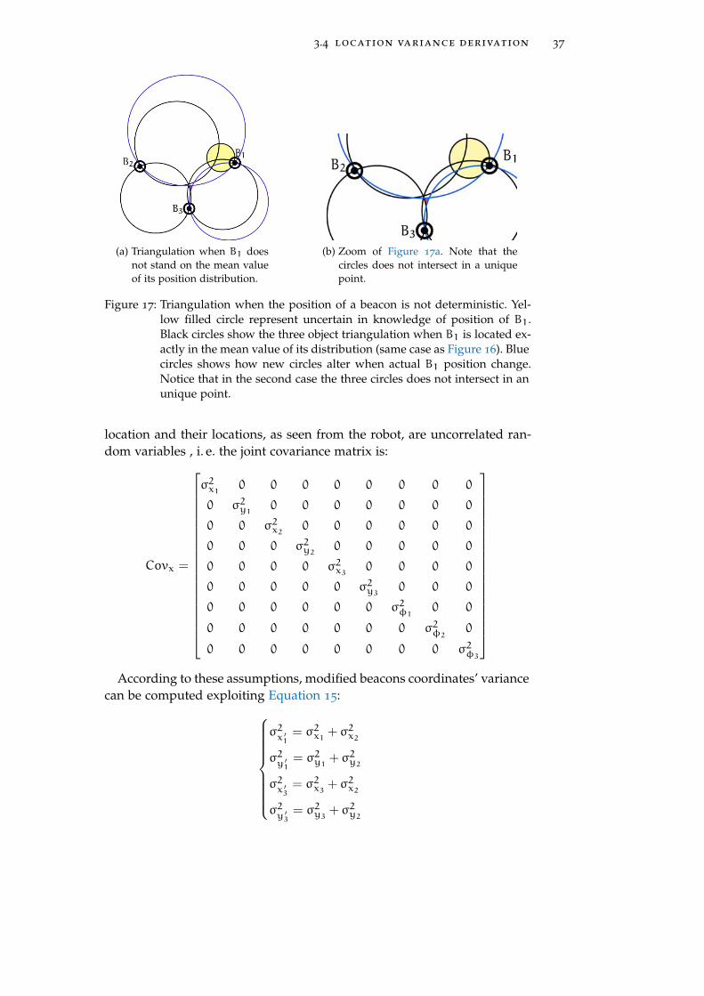
3.4 location variance derivation 37
(a) Triangulation when B1 doesnot stand on the mean valueof its position distribution.
(b) Zoom of Figure 17a. Note that thecircles does not intersect in a uniquepoint.
Figure 17: Triangulation when the position of a beacon is not deterministic. Yel-low filled circle represent uncertain in knowledge of position of B1.Black circles show the three object triangulation when B1 is located ex-actly in the mean value of its distribution (same case as Figure 16). Bluecircles shows how new circles alter when actual B1 position change.Notice that in the second case the three circles does not intersect in anunique point.
location and their locations, as seen from the robot, are uncorrelated ran-dom variables , i. e. the joint covariance matrix is:
Covx =
σ2x1 0 0 0 0 0 0 0 0
0 σ2y1 0 0 0 0 0 0 0
0 0 σ2x2 0 0 0 0 0 0
0 0 0 σ2y2 0 0 0 0 0
0 0 0 0 σ2x3 0 0 0 0
0 0 0 0 0 σ2y3 0 0 0
0 0 0 0 0 0 σ2φ1 0 0
0 0 0 0 0 0 0 σ2φ2 0
0 0 0 0 0 0 0 0 σ2φ3
According to these assumptions, modified beacons coordinates’ variance
can be computed exploiting Equation 15:
σ2x ′1
= σ2x1 + σ2x2
σ2y ′1
= σ2y1 + σ2y2
σ2x ′3
= σ2x3 + σ2x2
σ2y ′3
= σ2y3 + σ2y2
38 localization
Moreover, the expression for the variance of random variables Tij em-ployed in the second step of Algorithm 1, can be derived by using Equa-tion 19:
Var(T12) =[∂T12∂φ2
∂T12∂φ1
] [σ2φ2 0
0 σ2φ1
]∂T12∂φ2∂T12∂φ1
where,
∂T12∂φ2
=∂ cot(φ2 −φ1)
∂φ2= −
1
sin2(φ2 −φ1)
∂T12∂φ1
=∂ cot(φ2 −φ1)
∂φ1=
1
sin2(φ2 −φ1)
that leads to:
Var(T12) =σ2φ2
sin4(φ2 −φ1)+
σ2φ1
sin4(φ2 −φ1):= σ2T12
In a similar way, we can obtain for T23:
Var(T23) =σ2φ3
sin4(φ3 −φ2)+
σ2φ2
sin4(φ3 −φ2):= σ2T23 .
Then, computing:
∂T31∂T12
=−T23 − (1− T12T23)
(T12 + T23)2=
−T23(T12 − 1) − 1
(T12 + T23)2
∂T31∂T23
=T12 − (1− T12T23)
(T12 + T23)2=
−T12(T23 − T12) − 1
(T12 + T23)2
we obtain, for T31 :
Var(T31) =[∂T31∂T12
∂T31∂T23
] [σ2T12 0
0 σ2T23
][∂T31∂T12∂T31∂T23
]
= σ2T12
[T23(T12 − 1) − 1
(T12 + T23)2
]+ σ2T23
[T12(T23 − T12) − 1
(T12 + T23)2
]:= σ2T31 .
The third step of ToTal, provides for modified circle center coordinates.By using (19), it is possible to derive related variances:
σ2x ′12=[1 T12 y ′1
]σ2x ′1
0 0
0 σ2y ′1
0
0 0 σ2T12
1
T12
y ′1
= σ2x ′1
+ T212σ2y ′1
+ y2′1 σ
2T12
,
3.4 location variance derivation 39
σ2y ′12=[1 −T12 −x ′1
]σ2y ′1
0 0
0 σ2x ′1
0
0 0 σ2T12
1
−T12
−x ′1
= σ2y ′1
+ T212σ2x ′1
+ x2′1 σ
2T12
and, in a similar way for σ2x ′23
, σ2y ′23
, σ2x ′31
and σ2y ′31
:
σ2x ′23= σ2x ′3
+ T223σ2y ′3
+ y ′23 σ2T23
σ2y ′23= σ2y ′3
+ T223σ2x ′3
+ x ′23 σ2T23
σ2x ′31= σ2x ′3
+ σ2x ′1+ T231σ
2y ′3
+ y ′23 σ2T31
+ T231σ2y ′1
+ y2′1 σ
2T31
σ2y ′31= σ2y ′3
+ σ2y ′1+ T231σ
2x ′3
+ x ′23 σ2T31
+ T231σ2x ′1
+ x21σ2T31
Then, an expression for the variance of the parameter k ′31 can be com-puted:
σ2k ′31= x2
′1 σ
2x ′3
+ x2′3 σ
2x ′1
+ y2′1 σ
2y ′3
+ y2′3 σ
2y ′1+
+ (x ′1y′3)2σ2T31 + (T31y
′3)2σ2x ′1
+ (T31x′1)2σ2y ′3
+
+ (x ′3y′1)2σ2T31 + (T31y
′1)2σ2x ′3
+ (T31x′3)σ
2y ′1
and an expression for the variance of det(A):
σ2D = x2′12σ
2y ′23
+ y2′23σ
2x ′12
+ x2′12σ
2y ′31
+
+ y ′31σ2x ′12
+ x ′23σ2y ′23
+ y2′23σ
2x ′23
+
+ x2′23σ
2y ′31
+ y2′31σ
2x ′23
+ y2′12σ
2x ′23
+ x2′23σ
2y ′12
+
+ y2′12σ
2x ′31
+ x2′31σ
2y ′12
+ y2′23σ
2x ′23
+
+ x2′23σ
2y ′23
+ y2′23σ
2x ′31
+ x2′31σ
2y ′23
Finally, the variance of estimated position of the robot (xR,yR) can bederived. Let us define:
B =[1
y ′12−y′23
det(A)k ′31
det(A) −k ′31
det(A) −k ′31(y
′12−y
′23)
det(A)
]the variance for x-coordinate estimated position of the robot:
σ2xR = BT
σ2x ′2
σ2k ′31
σ2y ′12
σ2y ′23
σ2D
B =
= σ2x ′2+
(y ′12 − y
′23
det(A)
)2σ2k ′31
+ σ2y ′12
(k ′31
det(A)
)2+
+ σ2y ′23
(k ′31
det(A)
)2+
(k ′31(y
′12 − y
′23)
det(A)
)2σ2D (20)
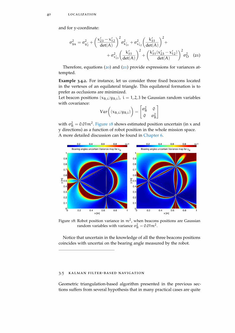
40 localization
and for y-coordinate:
σ2yR = σ2y ′2+
(x ′23 − x
′12
det(A)
)2σ2k ′31
+ σ2x ′12
(k ′31
det(A)
)2+
+ σ2x ′23
(k ′31
det(A)
)2+
(k ′31(x
′23 − x
′12)
det(A)
)2σ2D (21)
Therefore, equations (20) and (21) provide expressions for variances at-tempted.
Example 3.4.2. For instance, let us consider three fixed beacons locatedin the vertexes of an equilateral triangle. This equilateral formation is toprefer as occlusions are minimized.Let beacon positions (xB,i;yB,i), i = 1, 2, 3 be Gaussian random variableswith covariance:
Var
((xB,i;yB,i)
)=
[σ2B 0
0 σ2B
]with σ2B = 0.01m2. Figure 18 shows estimated position uncertain (in x andy directions) as a function of robot position in the whole mission space.A more detailed discussion can be found in Chapter 6.
Figure 18: Robot position variance in m2, when beacons positions are Gaussianrandom variables with variance σ2B = 0.01m2.
Notice that uncertain in the knowledge of all the three beacons positionscoincides with uncertai on the bearing angle measured by the robot.
3.5 kalman filter-based navigation
Geometric triangulation-based algorithm presented in the previous sec-tions suffers from several hypothesis that in many practical cases are quite
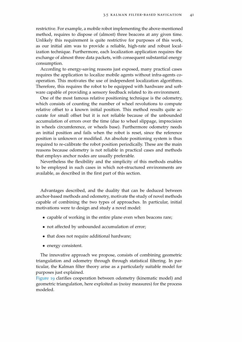
3.5 kalman filter-based navigation 41
restrictive. For example, a mobile robot implementing the above-mentionedmethod, requires to dispose of (almost) three beacons at any given time.Unlikely this requirement is quite restrictive for purposes of this work,as our initial aim was to provide a reliable, high-rate and robust local-ization technique. Furthermore, each localization application requires theexchange of almost three data packets, with consequent substantial energyconsumption.
According to energy-saving reasons just exposed, many practical casesrequires the application to localize mobile agents without infra-agents co-operation. This motivates the use of independent localization algorithms.Therefore, this requires the robot to be equipped with hardware and soft-ware capable of providing a sensory feedback related to its environment.
One of the most famous relative positioning technique is the odometry,which consists of counting the number of wheel revolutions to computerelative offset to a known initial position. This method results quite ac-curate for small offset but it is not reliable because of the unboundedaccumulation of errors over the time (due to wheel slippage, imprecisionin wheels circumference, or wheels base). Furthermore odometry needsan initial position and fails when the robot is reset, since the referenceposition is unknown or modified. An absolute positioning system is thusrequired to re-calibrate the robot position periodically. These are the mainreasons because odometry is not reliable in practical cases and methodsthat employs anchor nodes are usually preferable.
Nevertheless the flexibility and the simplicity of this methods enablesto be employed in such cases in which not-structured environments areavailable, as described in the first part of this section.
Advantages described, and the duality that can be deduced betweenanchor-based methods and odometry, motivate the study of novel methodscapable of combining the two types of approaches. In particular, initialmotivations were to design and study a novel model:
• capable of working in the entire plane even when beacons rare;
• not affected by unbounded accumulation of error;
• that does not require additional hardware;
• energy consistent.
The innovative approach we propose, consists of combining geometrictriangulation and odometry through through statistical filtering. In par-ticular, the Kalman filter theory arise as a particularly suitable model forpurposes just explained.Figure 19 clarifies cooperation between odometry (kinematic model) andgeometric triangulation, here exploited as (noisy measures) for the processmodeled.

42 localization
Figure 19: Novel approach proposed consists of combining geometric triangula-tion and odometry.
This approach has several advantages, such as robot’s displacements arenot required to be small and leads to an improvement in the hybrid useof the two methods, in particular triangulation could be used in biggerperiods or only when the estimate uncertain overcome a fixed threshold,in this way obtaining advantages of both methods.
The Extended Kalman filter EKF has been used as it raises as a naturalchoice in this context since it provides a convenient way to fuse the datafrom multiple sensors i.e. odometry and triangulation. While in generalthe theory of Kalman filtering requires the process to be modeled using alinear dynamic model and a linear output model, the EKF enables the useof non-linear equations. In this work, the dynamic model representing therobot’s wheels is nonlinear as better explained in Section 3.5.4.
In the following we propose, as an example, the modeling for a wheeledmobile robot and for a quadrotor. The model proposed for wheeled robotwill then exploited in Chapter 6 to perform numerical simulations.
3.5.1 Robot kinematic modeling
WMRs provide flexible motion capabilities to robotic systems, in particu-lar when we deal with reasonably smooth grounds and surfaces. Severalmobility configurations (wheel number and type, their location and actua-tion, single-body or multi-body vehicle structure) can be chosen accordingto specific applications. The most common for single-body robots are differ-ential drive and synchro drive, tricycle or car-like drive, omnidirectional steeringetc.. Detailed reference on the analytic study of the kinematics of WMRs is[1].
Quadrotors also have become a widely used platform for many applica-tions that include both indoor and outdoor. High performance combinedwith an increasing availability and reduced prices have led to a growinginterest in using rotor based platforms.
In the following the kinematic models of two different types of widelyused robots are presented. Kinematics is the study of geometry of mo-tion. In the context of mobile robots, we are interested in determining themotion of the robot from the geometry of the constraint imposed by the
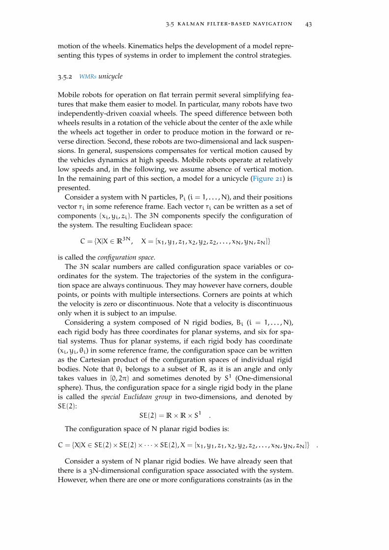
3.5 kalman filter-based navigation 43
motion of the wheels. Kinematics helps the development of a model repre-senting this types of systems in order to implement the control strategies.
3.5.2 WMRs unicycle
Mobile robots for operation on flat terrain permit several simplifying fea-tures that make them easier to model. In particular, many robots have twoindependently-driven coaxial wheels. The speed difference between bothwheels results in a rotation of the vehicle about the center of the axle whilethe wheels act together in order to produce motion in the forward or re-verse direction. Second, these robots are two-dimensional and lack suspen-sions. In general, suspensions compensates for vertical motion caused bythe vehicles dynamics at high speeds. Mobile robots operate at relativelylow speeds and, in the following, we assume absence of vertical motion.In the remaining part of this section, a model for a unicycle (Figure 21) ispresented.
Consider a system with N particles, Pi (i = 1, . . . ,N), and their positionsvector ri in some reference frame. Each vector ri can be written as a set ofcomponents (xi,yi, zi). The 3N components specify the configuration ofthe system. The resulting Euclidean space:
C = X|X ∈ R3N, X = [x1,y1, z1, x2,y2, z2, . . . , xN,yN, zN]
is called the configuration space.The 3N scalar numbers are called configuration space variables or co-
ordinates for the system. The trajectories of the system in the configura-tion space are always continuous. They may however have corners, doublepoints, or points with multiple intersections. Corners are points at whichthe velocity is zero or discontinuous. Note that a velocity is discontinuousonly when it is subject to an impulse.
Considering a system composed of N rigid bodies, Bi (i = 1, . . . ,N),each rigid body has three coordinates for planar systems, and six for spa-tial systems. Thus for planar systems, if each rigid body has coordinate(xi,yi, θi) in some reference frame, the configuration space can be writtenas the Cartesian product of the configuration spaces of individual rigidbodies. Note that θi belongs to a subset of R, as it is an angle and onlytakes values in [0, 2π) and sometimes denoted by S1 (One-dimensionalsphere). Thus, the configuration space for a single rigid body in the planeis called the special Euclidean group in two-dimensions, and denoted bySE(2):
SE(2) = R×R× S1 .
The configuration space of N planar rigid bodies is:
C = X|X ∈ SE(2)×SE(2)×· · ·×SE(2),X = [x1,y1, z1, x2,y2, z2, . . . , xN,yN, zN] .
Consider a system of N planar rigid bodies. We have already seen thatthere is a 3N-dimensional configuration space associated with the system.However, when there are one or more configurations constraints (as in the
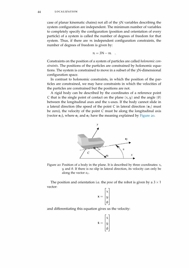
44 localization
case of planar kinematic chains) not all of the 3N variables describing thesystem configuration are independent. The minimum number of variablesto completely specify the configuration (position and orientation of everyparticle) of a system is called the number of degrees of freedom for thatsystem. Thus, if there are m independent configuration constraints, thenumber of degrees of freedom is given by:
n = 3N−m .
Constraints on the position of a system of particles are called holonomic con-straints. The positions of the particles are constrained by holonomic equa-tions. The system is constrained to move in a subset of the 3N-dimensionalconfiguration space.
In contrast to holonomic constraints, in which the position of the par-ticles are constrained, we may have constraints in which the velocities ofthe particles are constrained but the positions are not.
A rigid body can be described by the coordinates of a reference pointC that is the single point of contact on the plane (x,y) and the angle (θ)
between the longitudinal axes and the x-axes. If the body cannot slide ina lateral direction (the speed of the point C in lateral direction (el) mustbe zero), the velocity of the point C must be along the longitudinal axis(vector ef), where el and ef have the meaning explained by Figure 20.
Figure 20: Position of a body in the plane. It is described by three coordinates: x,y and θ. If there is no slip in lateral direction, its velocity can only bealong the vector ef.
The position and orientation i.e. the pose of the robot is given by a 3× 1vector:
x =
xyθ
and differentiating this equation gives us the velocity:
x =
xyθ
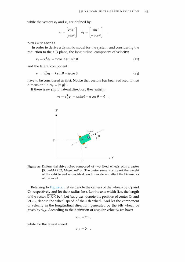
3.5 kalman filter-based navigation 45
while the vectors ef and el are defined by:
ef =
[cos θ
sin θ
]el =
[sin θ
− cos θ
].
dynamic model
In order to derive a dynamic model for the system, and considering thereduction to the 2-D plane, the longitudinal component of velocity:
vf = vTcef = x cos θ+ y sin θ (22)
and the lateral component :
vl = vTcel = x sin θ− y cos θ (23)
have to be considered as first. Notice that vectors has been reduced to twodimension i. e. vc = [x y]T .
If there is no slip in lateral direction, they satisfy:
vl = vTcel = x sin θ− y cos θ = 0 .
Figure 21: Differential drive robot composed of two fixed wheels plus a castor[SuperMARIO, MagellanPro]. The castor serve to support the weightof the vehicle and under ideal conditions do not affect the kinematicsof the robot.
Referring to Figure 21, let us denote the centers of the wheels by C1 andC2 respectively and let their radius be r. Let the axis width (i. e. the lengthof the vector
−−−→C1C2) be l. Let (xi,yi, zi) denote the position of center Ci and
let ωi denote the wheel speed of the i-th wheel. And let the componentof velocity in the longitudinal direction, generated by the i-th wheel, begiven by vf,i. According to the definition of angular velocity, we have:
vf,i = rωi
while for the lateral speed:vl,i = 0 .
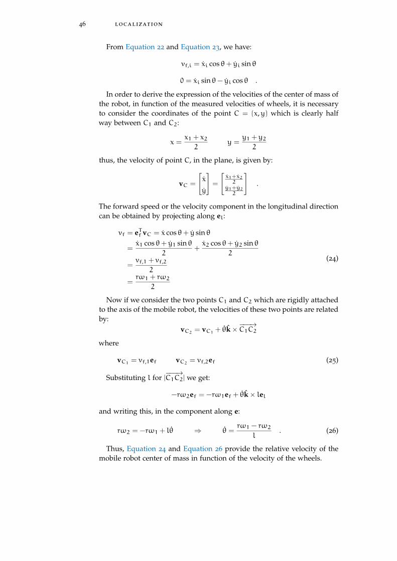
46 localization
From Equation 22 and Equation 23, we have:
vf,i = xi cos θ+ yi sin θ
0 = xi sin θ− yi cos θ .
In order to derive the expression of the velocities of the center of mass ofthe robot, in function of the measured velocities of wheels, it is necessaryto consider the coordinates of the point C = (x,y) which is clearly halfway between C1 and C2:
x =x1 + x22
y =y1 + y22
thus, the velocity of point C, in the plane, is given by:
vC =
[x
y
]=
[x1+x22
y1+y22
].
The forward speed or the velocity component in the longitudinal directioncan be obtained by projecting along el:
vf = eTf vC = x cos θ+ y sin θ
=x1 cos θ+ y1 sin θ
2+x2 cos θ+ y2 sin θ
2
=vf,1 + vf,2
2
=rω1 + rω2
2
(24)
Now if we consider the two points C1 and C2 which are rigidly attachedto the axis of the mobile robot, the velocities of these two points are relatedby:
vC2 = vC1 + θk×−−−→C1C2
where
vC1 = vf,1ef vC2 = vf,2ef (25)
Substituting l for |−−−→C1C2| we get:
−rω2ef = −rω1ef + θk× lel
and writing this, in the component along e:
rω2 = −rω1 + lθ ⇒ θ =rω1 − rω2
l. (26)
Thus, Equation 24 and Equation 26 provide the relative velocity of themobile robot center of mass in function of the velocity of the wheels.
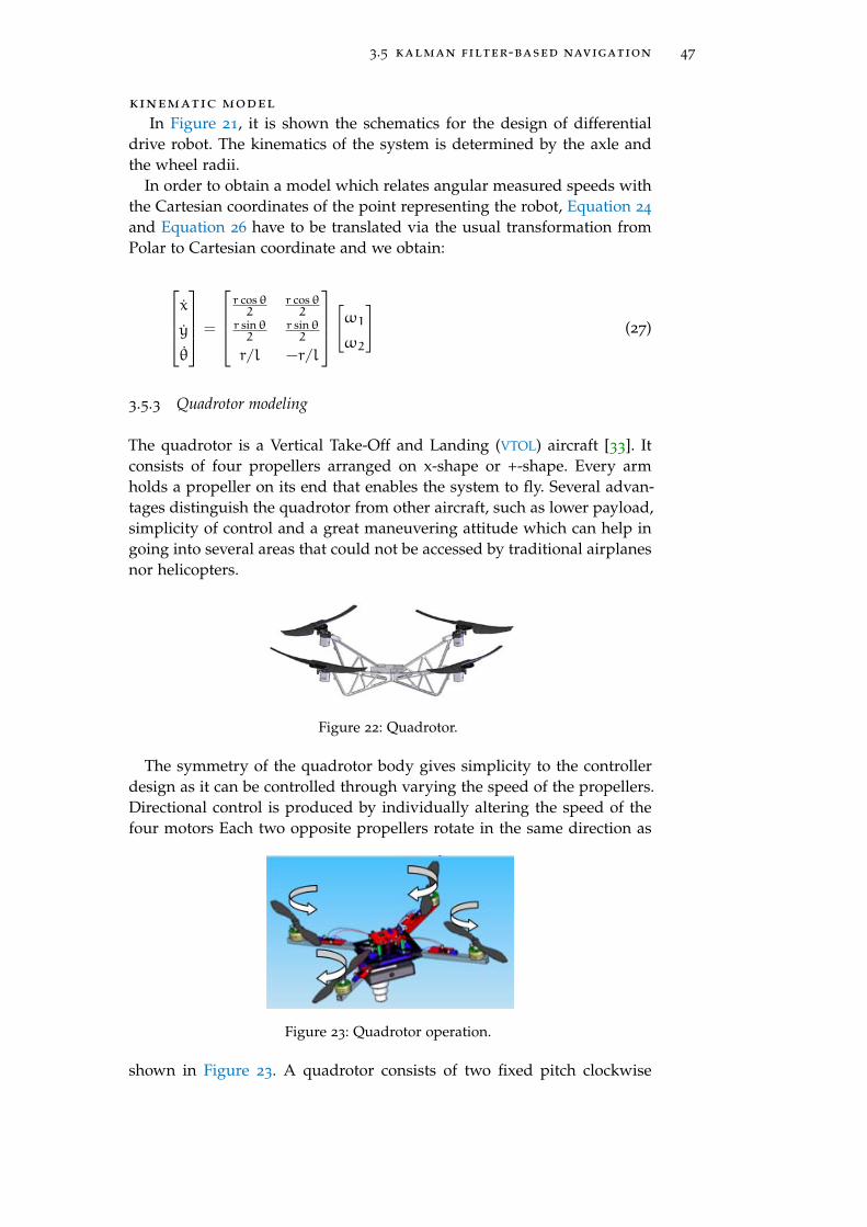
3.5 kalman filter-based navigation 47
kinematic model
In Figure 21, it is shown the schematics for the design of differentialdrive robot. The kinematics of the system is determined by the axle andthe wheel radii.
In order to obtain a model which relates angular measured speeds withthe Cartesian coordinates of the point representing the robot, Equation 24
and Equation 26 have to be translated via the usual transformation fromPolar to Cartesian coordinate and we obtain:
xyθ
=
r cosθ2
r cosθ2
r sinθ2
r sinθ2
r/l −r/l
[ω1
ω2
](27)
3.5.3 Quadrotor modeling
The quadrotor is a Vertical Take-Off and Landing (VTOL) aircraft [33]. Itconsists of four propellers arranged on x-shape or +-shape. Every armholds a propeller on its end that enables the system to fly. Several advan-tages distinguish the quadrotor from other aircraft, such as lower payload,simplicity of control and a great maneuvering attitude which can help ingoing into several areas that could not be accessed by traditional airplanesnor helicopters.
Figure 22: Quadrotor.
The symmetry of the quadrotor body gives simplicity to the controllerdesign as it can be controlled through varying the speed of the propellers.Directional control is produced by individually altering the speed of thefour motors Each two opposite propellers rotate in the same direction as
Figure 23: Quadrotor operation.
shown in Figure 23. A quadrotor consists of two fixed pitch clockwise
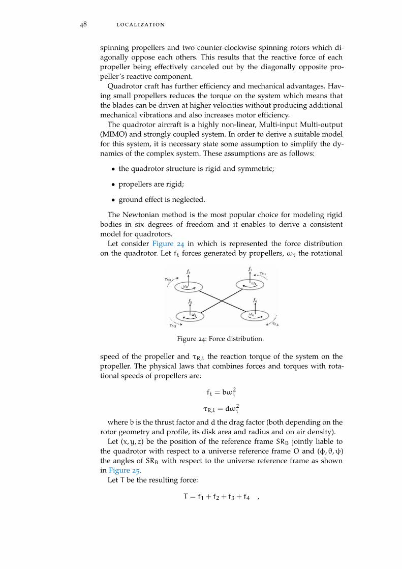
48 localization
spinning propellers and two counter-clockwise spinning rotors which di-agonally oppose each others. This results that the reactive force of eachpropeller being effectively canceled out by the diagonally opposite pro-peller’s reactive component.
Quadrotor craft has further efficiency and mechanical advantages. Hav-ing small propellers reduces the torque on the system which means thatthe blades can be driven at higher velocities without producing additionalmechanical vibrations and also increases motor efficiency.
The quadrotor aircraft is a highly non-linear, Multi-input Multi-output(MIMO) and strongly coupled system. In order to derive a suitable modelfor this system, it is necessary state some assumption to simplify the dy-namics of the complex system. These assumptions are as follows:
• the quadrotor structure is rigid and symmetric;
• propellers are rigid;
• ground effect is neglected.
The Newtonian method is the most popular choice for modeling rigidbodies in six degrees of freedom and it enables to derive a consistentmodel for quadrotors.
Let consider Figure 24 in which is represented the force distributionon the quadrotor. Let fi forces generated by propellers, ωi the rotational
Figure 24: Force distribution.
speed of the propeller and τR,i the reaction torque of the system on thepropeller. The physical laws that combines forces and torques with rota-tional speeds of propellers are:
fi = bω2i
τR,i = dω2i
where b is the thrust factor and d the drag factor (both depending on therotor geometry and profile, its disk area and radius and on air density).
Let (x,y, z) be the position of the reference frame SRB jointly liable tothe quadrotor with respect to a universe reference frame O and (φ, θ,ψ)the angles of SRB with respect to the universe reference frame as shownin Figure 25.
Let T be the resulting force:
T = f1 + f2 + f3 + f4 ,
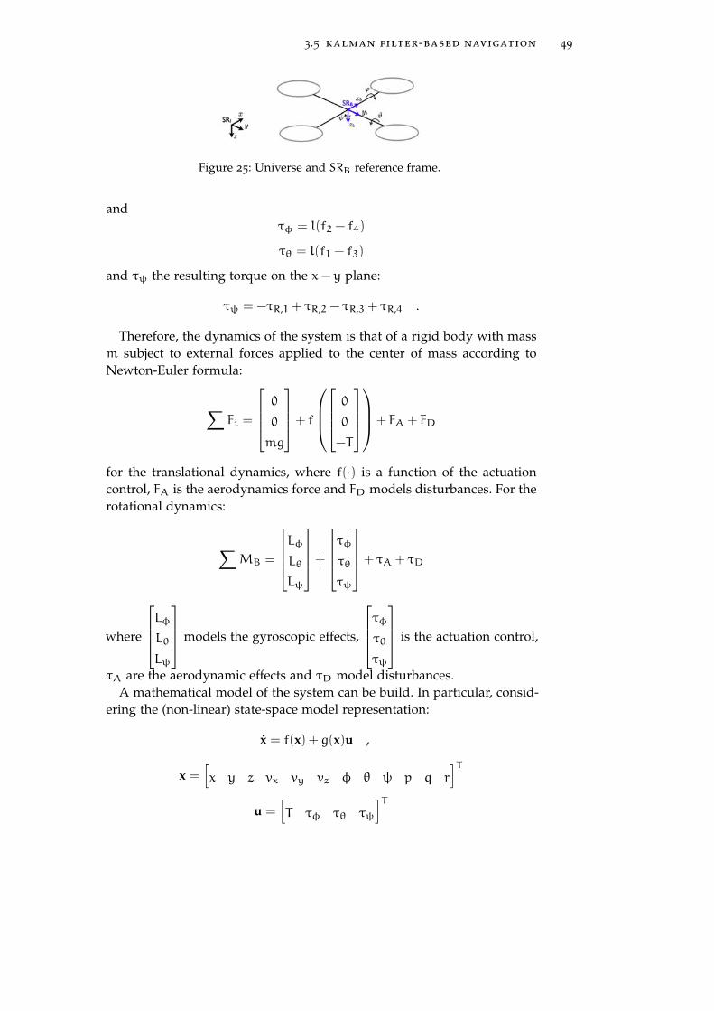
3.5 kalman filter-based navigation 49
Figure 25: Universe and SRB reference frame.
andτφ = l(f2 − f4)
τθ = l(f1 − f3)
and τψ the resulting torque on the x− y plane:
τψ = −τR,1 + τR,2 − τR,3 + τR,4 .
Therefore, the dynamics of the system is that of a rigid body with massm subject to external forces applied to the center of mass according toNewton-Euler formula:
∑Fi =
0
0
mg
+ f
00−T
+ FA + FD
for the translational dynamics, where f(·) is a function of the actuationcontrol, FA is the aerodynamics force and FD models disturbances. For therotational dynamics:
∑MB =
LφLθLψ
+
τφτθτψ
+ τA + τD
where
LφLθLψ
models the gyroscopic effects,
τφτθτψ
is the actuation control,
τA are the aerodynamic effects and τD model disturbances.A mathematical model of the system can be build. In particular, consid-
ering the (non-linear) state-space model representation:
x = f(x) + g(x)u ,
x =[x y z vx vy vz φ θ ψ p q r
]Tu =
[T τφ τθ τψ
]T

50 localization
the model:
x = vx
y = vy
z = vz
vx = FA,x − (cosψ sin θ cosφ+ sinψ sinφ) Tm
vy = FA,y − (sinψ sin θ cosφ+ sinφ cosψ) Tm
vz = FA,x + g− cos θ cosφ Tm
φ = p+ sinφ tan θq+ cosφ tan θr
θ = cosφq− sinφr
ψ = sinφ sec θq+ cosφ sec θr
p = τA,x +IrIxqΩr +
Iy−IzIx
qr+τφIx
q = τA,y +IrIypΩr +
Iz−IxIy
pr+ τθIy
r = τA,z +Ix−IyIz
pq+τψIz
where have been used Ir for the blades inertia and Ωr for the averageblades rotation velocity.
3.5.4 The Extended Kalman Filter
In order to combine the data from odometry readings together with trian-gulation results, a kinematic model for the robot is necessary.
In the following, the model for a unicycle has been chosen for instance,but any other model for mobile robots (e. g. quadrotor) is suitable for thealgorithm with no others complications, as in general all these models arenon-linear. The model in state space representation for the process is:x(k+ 1) = f(x(k), u(k)) + w(k)
y(k) = h(x(k)) + v(k)(28)
where f(x(k), u(k)) is the nonlinear state transition function of the robot.In general w(k) ∼ N(0,Rw) is a Gaussian noise with zero mean and covari-ance Rw independent from k. h(x(k)) is the nonlinear observation modeland v(k) is a Gaussian noise with zero mean and covariance Rv(k). It isimportant to notice that the model noise w(k) has covariance matrix in-dependent from the current step k. In fact, while the model noise is ingeneral a stationary random process, the measure noise v(k) has covari-ance function that depends on the position of the robot with respect tobeacons position. For this reason, it is necessary to consider a covariancein function of the time step k.
Our approach consists in considering:
• odometry follows the kinematic model, that is the function f(·) in(28);
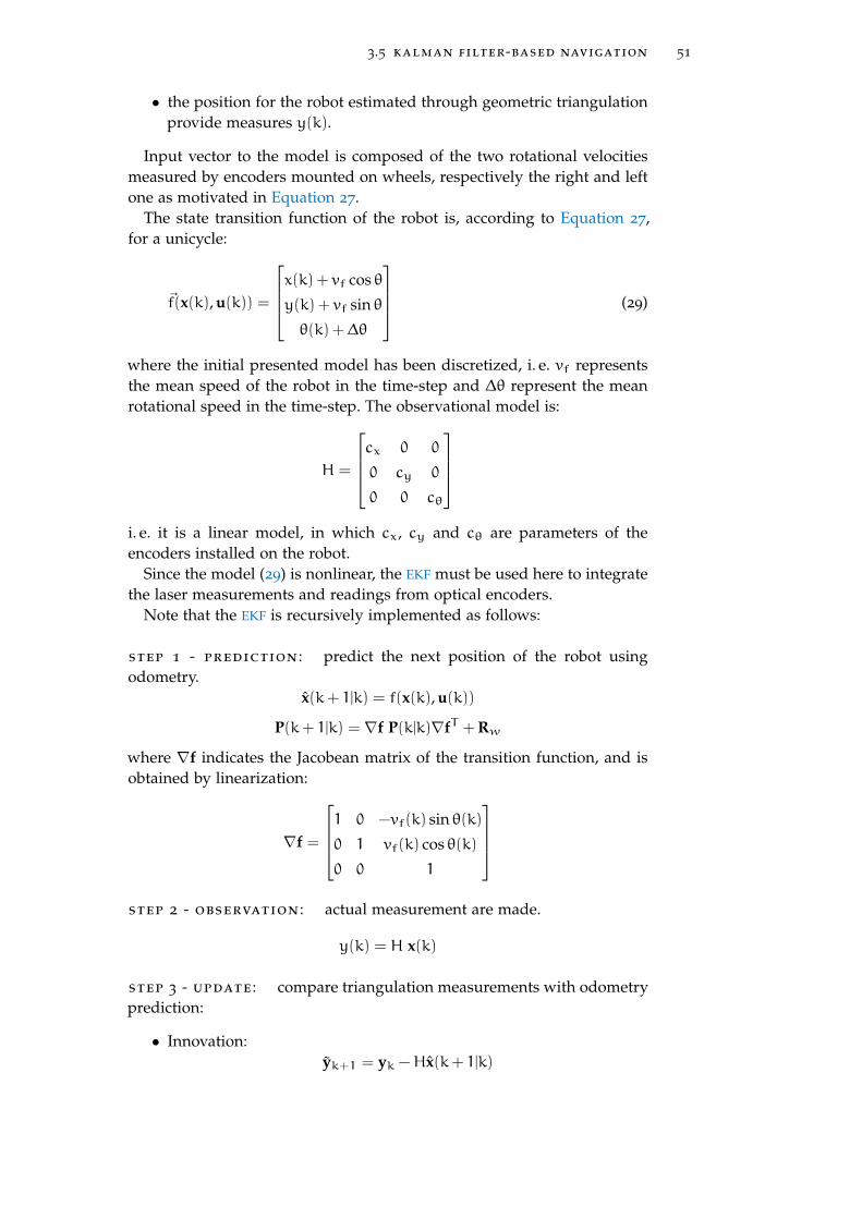
3.5 kalman filter-based navigation 51
• the position for the robot estimated through geometric triangulationprovide measures y(k).
Input vector to the model is composed of the two rotational velocitiesmeasured by encoders mounted on wheels, respectively the right and leftone as motivated in Equation 27.
The state transition function of the robot is, according to Equation 27,for a unicycle:
~f(x(k), u(k)) =
x(k) + vf cos θ
y(k) + vf sin θ
θ(k) +∆θ
(29)
where the initial presented model has been discretized, i. e. vf representsthe mean speed of the robot in the time-step and ∆θ represent the meanrotational speed in the time-step. The observational model is:
H =
cx 0 0
0 cy 0
0 0 cθ
i. e. it is a linear model, in which cx, cy and cθ are parameters of theencoders installed on the robot.
Since the model (29) is nonlinear, the EKF must be used here to integratethe laser measurements and readings from optical encoders.
Note that the EKF is recursively implemented as follows:
step 1 - prediction : predict the next position of the robot usingodometry.
x(k+ 1|k) = f(x(k), u(k))
P(k+ 1|k) = ∇f P(k|k)∇fT + Rw
where ∇f indicates the Jacobean matrix of the transition function, and isobtained by linearization:
∇f =
1 0 −vf(k) sin θ(k)
0 1 vf(k) cos θ(k)
0 0 1
step 2 - observation : actual measurement are made.
y(k) = H x(k)
step 3 - update : compare triangulation measurements with odometryprediction:
• Innovation:yk+1 = yk −Hx(k+ 1|k)
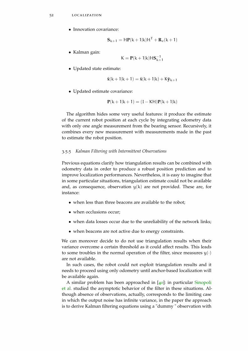
52 localization
• Innovation covariance:
Sk+1 = HP(k+ 1|k)HT + Rv(k+ 1)
• Kalman gain:K = P(k+ 1|k)HS−1
k+1
• Updated state estimate:
x(k+ 1|k+ 1) = x(k+ 1|k) +Kyk+1
• Updated estimate covariance:
P(k+ 1|k+ 1) = (I−KH)P(k+ 1|k)
The algorithm hides some very useful features: it produce the estimateof the current robot position at each cycle by integrating odometry datawith only one angle measurement from the bearing sensor. Recursively, itcombines every new measurement with measurements made in the pastto estimate the robot position.
3.5.5 Kalman Filtering with Intermittent Observations
Previous equations clarify how triangulation results can be combined withodometry data in order to produce a robust position prediction and toimprove localization performances. Nevertheless, it is easy to imagine thatin some particular situations, triangulation estimate could not be availableand, as consequence, observation y(k) are not provided. These are, forinstance:
• when less than three beacons are available to the robot;
• when occlusions occur;
• when data losses occur due to the unreliability of the network links;
• when beacons are not active due to energy constraints.
We can moreover decide to do not use triangulation results when theirvariance overcome a certain threshold as it could affect results. This leadsto some troubles in the normal operation of the filter, since measures y(·)are not available.
In such cases, the robot could not exploit triangulation results and itneeds to proceed using only odometry until anchor-based localization willbe available again.
A similar problem has been approached in [40]: in particular Sinopoliet al. studied the asymptotic behavior of the filter in these situations. Al-though absence of observations, actually, corresponds to the limiting casein which the output noise has infinite variance, in the paper the approachis to derive Kalman filtering equations using a "dummy " observation with
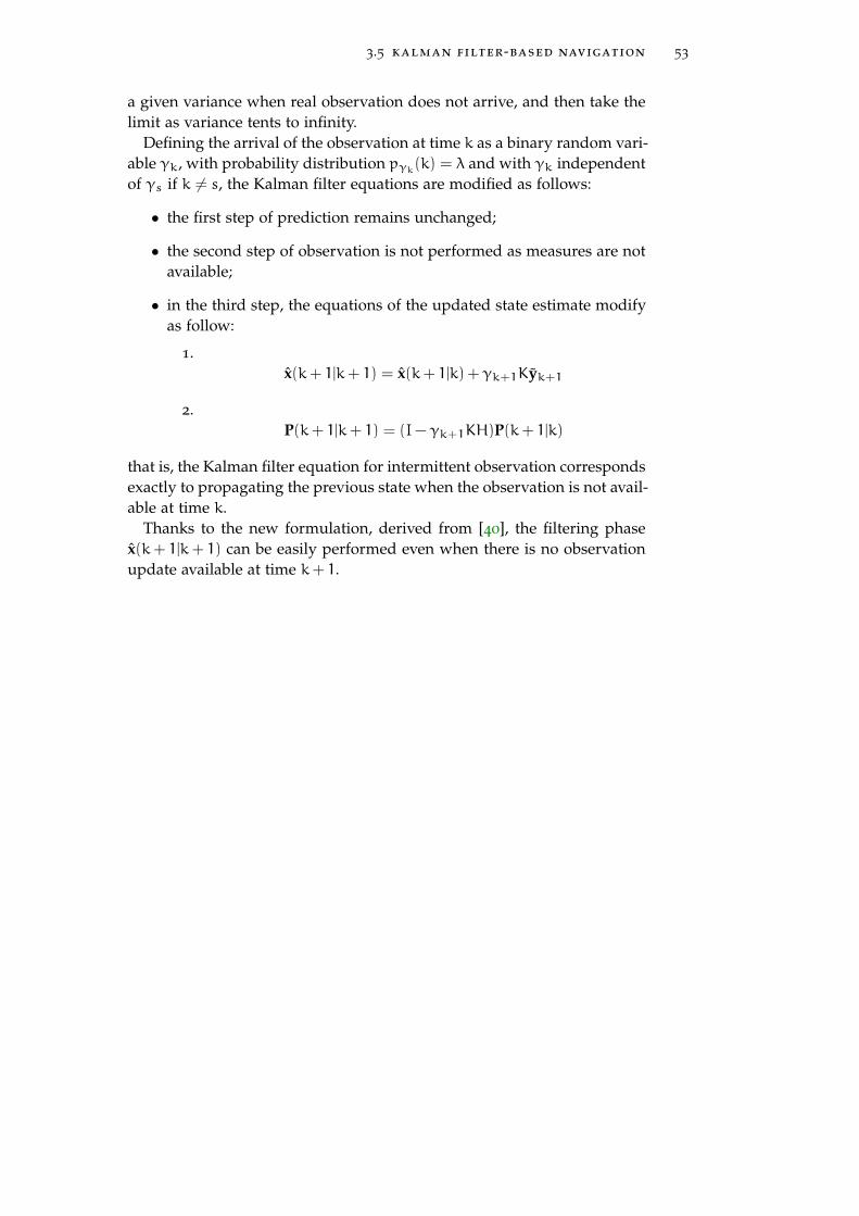
3.5 kalman filter-based navigation 53
a given variance when real observation does not arrive, and then take thelimit as variance tents to infinity.
Defining the arrival of the observation at time k as a binary random vari-able γk, with probability distribution pγk(k) = λ and with γk independentof γs if k 6= s, the Kalman filter equations are modified as follows:
• the first step of prediction remains unchanged;
• the second step of observation is not performed as measures are notavailable;
• in the third step, the equations of the updated state estimate modifyas follow:
1.x(k+ 1|k+ 1) = x(k+ 1|k) + γk+1Kyk+1
2.P(k+ 1|k+ 1) = (I− γk+1KH)P(k+ 1|k)
that is, the Kalman filter equation for intermittent observation correspondsexactly to propagating the previous state when the observation is not avail-able at time k.
Thanks to the new formulation, derived from [40], the filtering phasex(k+ 1|k+ 1) can be easily performed even when there is no observationupdate available at time k+ 1.

4B E A C O N D E P L O Y M E N T F O R L O C A L I Z AT I O N
Multiple are the advantages introduced thanks to the interplay betweenfixed and mobile agents: for instance, as introduced in previous section,static sensors can provide localization services, while at the same timerobotic nodes deal with sensing the environment. Although many worksin literature treat pre-configured networks of fixed nodes, because of pre-existing infrastructures or constraints due to physical issues, there existsome practical cases that envisage the network to automatically adapt toenvironments, a-priori unknown.The beacon deployment process regards the problem of optimally deployingbeacons, in order to provide mutual services to the robotic network.
Beacon displacement strongly affects quality of localization and manyother services provided by the network. For instance, when consideringthe simple triangulation problem described in Chapter 3: the number ofvisible beacons and their placement geometry is crucial in order to reachreliable results. Each node in fact requires almost three beacons to be ableto localize itself.
This chapter aims to study approaches to sensor node localization thatuses sequentially deployed beacons in order to localize mobile agents.
4.1 objective and motivation
In this section the main motivations to the work are introduced and the ob-jective are described in detail. Moreover the key contributions are resumed.A detailed previous-work description concludes the section.
4.1.1 Problem definition
In this chapter the motivation, design, implementation and evaluation ofa sequentially self-deployment system based on triangulation is presented.The main purposes of this work are threefold:
• to formalize the sensor placement problem;
• to address beacon deployment issues, following the idea of the novelconcept of self-configuring beacon network;
• to propose a novel method capable of determining locations for newbeacons to be deployed in an optimal way, by exploiting resultspresented in Chapter 3 regarding geometric triangulation variancederivation;
55

56 beacon deployment for localization
4.1.2 Previous work
Much of the research conduced thus far has mainly focused on localizationtechniques, while beacon placement issues have not been rather explored.Typical approaches taken in literature deal with pre-existing beacons dis-placement, thus focusing on optimal selection between available beacons.An adaptive beacon placement algorithm has been proposed in [3], wherebeacons are deployed sequentially basing on empirically data of the per-ceived localization error. The perceived error is obtained by observationsamong neighboring beacons. When beacons are densely deployed over anarea, the perceived localization error among them should reflect the errorcharacteristics of the terrain or environment, which can then be applied toestimate the localization error of the actual sensor nodes.Further work in [3] by Bulusu et al. provides a framework to realize theadaptive algorithm in the real world by proposing a distributed algorithmto disseminate the perceived localization error into a centralized location.Isler describe a beacon deployment strategy with a different objective: min-imizing the number of deployed beacons to localize mobile objects. Theproblem approached deals with finding the minimum number and theplacement of cameras so that the error in localization is less then an errorthreshold at every point in the workspace.In [41] the problem of controlling the configuration of a sensor team whichemploy triangulation for estimation is studied. Authors present a particlefilter. The approach provide the optimal move at each time step by com-puting numerically an n-dimensional gradient. This work solves a localplacement problem for a small number of robots at each time step.In [32], the problem of relocating a sensor team whose members are re-stricted to lie on a circle and charged with jointly estimating the locationof the target was studied. Efrat et al. in [14] study the problem of placingcameras in a polygonal workspace in such a way that for each point ofinterest, there are two cameras which can view the point at an acceptableangle. The work in [22] studies the problem of assigning disjoint pairs ofsensors to targets.In the work proposed by Tekdas and Isler, a solution framework basedon integer linear programming is proposed. The work [22] proposes more-over an approximation algorithm with a constant factor performance guar-antee, while the main focus addressed is the minimization of the numberof sensors employed.
4.1.3 Contributions
The key contributions of this work consists in introducing optimal beacondeployment criteria and algorithms for geometric triangulation.In the first part of this section, we propose a sequentially self-deploymentsystem capable of optimally locate new beacons that provides localizationservices for robotic networks.First of all, we introduce the problem by describing how a-priori designed
4.1 objective and motivation 57
patterns can optimally cover the mission space by minimizing the numberof beacons involved.Subsequently, according to robustness and autonomy constraints, we pro-ceed in developing mechanism that make the network capable of comput-ing locations for new beacons to be deployed in an accurate manner.
Our method is based on cooperation between pre-existing beacons: thanksto local exchange of information, candidates location for new beacons arecomputed through local optimization. Computed positions are then trans-mitted to robotic agents for deployment.
4.1.4 Problem formulation
In this section, the sensor placement problem for triangulation-based lo-calization is formulated.Given a workspace Ω, which consists of all possible locations for the tar-get, let s be a k-tuple representing related sensor parameters which caninclude, for example, location and orientation of agents. Let Q be the do-main of s. Q represents the set of all possible placements of a single sensorin Ω.
Let us consider a function U:
U : Q×Q×Q×Ω → R
U(si, sj, sk,ω) returns the uncertainty in localizing a target positioned atω (ω ∈ Ω) exploiting three sensors located and orientated as described bysi, sj and sk respectively.It is easy to deduce that the function U is specific to particular environ-ment and sensing models. For example, U(si, sj, sk,ω) can be infinite ifthe environment causes an occlusion between ω and either si or sj or sk.
Let S = s1, . . . , sn ⊆ Qn be a placement of sensors where the ith
sensor has parameters si. The quality of a placement in a workspace isdetermined as follows:
U(S,Ω) = maxω∈Ω
minsi,sj,sk∈S
U(si, sj, sk,ω) (30)
Equation 30 explains how, to establish the quality of services provided bya given beacons arrangement, the largest uncertain value over the entireworkspace is taken.
The optimal sensor placement problem can be formulated as follow:
Definition 4.1. Given a workspaceΩ, candidate sensor locations Q and anuncertain function U, find a placement S with minimum cardinality suchthat minimize U, i. e. :
minS⊆Qn
U(S,Ω)
The definition clarify the twofold objectives:
• raising a placement that minimize the number of sensors employed;
• minimizing the uncertain in estimated position.
58 beacon deployment for localization
In addition, we underline that at low and medium beacon densities, thequality of localization suffers due to poor placement of beacons; while athigh densities collisions in communications compromises the scalability ofperformances. Hereafter we present an example that clarify this seemingcounter-sense.
4.1.5 Sensor placement problem for triangulation-based localization is NP-Complete
Unfortunately optimal solution to (30), i. e. optimal beacons displacementthat both minimizes sensors employed and guarantee minimal localizationuncertain is not trivial. It is furthermore possible to state that this kind ofproblems are NP-Complete1.
This fact is usually demonstrated in literature [43] by establishing itsrelation to the well-known k-center problem, which is NP-Complete.
In the k-center problem, we are given a set of locations for centers and aset of targets along with a distance function d(i, j) between the centers andthe targets. The objective is to minimize the maximum distance betweenany target and the center closest to it. The converse problem, where themaximum distance from each vertex to its center is given and the numberof centers is to be minimized, is also NP-Complete. Hence, the sensorplacement problem is, at least, as hard as the converse k-center problem.
4.2 introduction on adaptive beacon placement
Intuitively, approaches such as uniform and very dense beacon placementare suitable for many practical approaches. However there exist some dis-advantages that compromise their effectiveness.First of all, uniform placement results as a good strategy in many cases inwhich we do not dispose of any detailed information about the work to ac-complish or the environment to study. However, this model is insufficientdue to the following reasons:
• Beacons may be perturbed during deployment. Consider for exam-ple, a terrain comprising hilltops. Air dropped beacon will roll overthe hill compromising the overall network characteristics.
• Even when beacon placement is uniform, noise may affect the visi-bility of beacons that should be in range: in fact, uneven terrains andobstacles bring additional uncertainty.
Very dense placement may not be a viable solution too. This because ofseveral reasons:
• Signals interference.
1 A decision problem is NP-Complete when it is both in NP and NP-Hard. The most notablecharacteristic of NP-Complete problems is that no fast solution to them is known. That is,the time required to solve the problem using any currently known algorithm increasesvery quickly as the size of the problem grows.
4.2 introduction on adaptive beacon placement 59
• Cost and power: cost of the beacons may preclude very dense place-ment. Power considerations may require that only a restricted sub-sets of the beacon network can be active at any given time.
• The environmental or terrain conditions may be such that even in-creasing the density uniformly will not overcome the problem. Forinstance, if the number of dropped beacons were doubled, the samesituation would persist. Also, the terrain can already have a veryhigh density of beacons and hence the new beacons deployed mustbe added in particular places to cope with noise.
• At very high densities, the phenomenon of self-interference emerges.In fact, the probability of collisions among signals transmitted by thebeacons increases.
The fundamental limitation of the two proposed approaches is that theyare basically fixed strategies, that do not take into account environmentalconditions that cannot be known a-priori. It is practically impossible topre-configure to such terrain and propagation uncertainties and computean ideal beacon placement that uniformly achieves a desired quality oflocalization across the region.Beacon placement needs to adapt to the noisy and unpredictable environ-mental conditions. Thus, recent studies addresses the problem of Adaptivebeacon placement. The problem deals with understanding how should ad-ditional beacons be placed, given an existing field of beacons, in order toreach best localization performances.
Bulusu et al. in [3] has formalized two simple algorithms for adaptivebeacon placement. The procedures differ in the amount of global knowl-edge and processing used to take decisions.
4.2.0.1 Random
The simplest algorithm for beacon deployment provide nodes to do notpay attention to the quality of localization at different areas of the missionspace and simply selects a random point in the region as a candidate foradding a new beacon. The algorithm is structured as proposed in Algo-rithm 2.
Algorithm 2 Random beacon deployment algorithm
1) Select a random point (x∗,y∗)2) Add a new beacon at (x∗,y∗)
The presented model is extremely simple, however it is usually takeninto account as it is similar in character to uncontrolled airdrop of addi-tional nodes. Its complexity is O(1).
4.2.0.2 Max
The Max algorithm is described in Algorithm 3
60 beacon deployment for localization
Algorithm 3 Max algorithm
Let the terrain be a a square of s meters and each robot take measuresin ρ meters.1) Divide the terrain into ρ× ρ squares.2) Measure localization error at each point in the terrain that corre-sponds to a square.3) Add a new beacon at the point (x∗,y∗) that has the highest measuredlocalization error among all points.
This algorithm is based on the assumption that points with high local-ization error are spatially correlated. The advantage of this algorithm isthat it can be computed in a very straightforward way; however it may beinfluenced by random noise or propagation effects.The complexity of the Max algorithm is linear in the number of square ofthe discretization.
Algorithm proposed beforehand, have been reported in order to providean overview on fixed strategies. For a comprehensive discussion aboutuniform and very dense placements, please refer to [3].
4.3 adaptive beacon deployment based on triangulation vari-ance map
It is possible to state that many of the techniques proposed in literaturefor landmarks positioning are specific of the localization method exploited,Moreover, as previously demonstrated, the problem of optimal beacon de-ployment for triangulation is NP-Complete.These reasons have directed researchers to develop models that make useof pre-existing beacon networks, and directing their attentions on selectingthe more appropriate tern of beacon to perform the triangulation, whenmobile agents are capable of sensing more than three beacons.This approach is based on a strong assumption: the beacon network islocated in an off-line manner, and there is redundancy in beacons deploy-ment. However we can deduce that this perspective is not suitable forsuch cases in which we cannot dispose a priori of information regardingthe mission space. In such cases mobile agents are required to providean adapting structure the the sensor network, through deploying beaconsbasing on sensed environment.
This chapter presents a novel approach for beacon deployment based ontriangulation variance estimation described in previous Chapter 3.In particular the uncertain about self actual location of new deployed bea-cons will provide a suitable and robust criteria for the iterative design oftheir locations.
In the following, two main assumption are done:
• triangulation is used as localization method. As previously intro-duced, the beacons deployment problem is specific for the localiza-tion methods used, and this assumption specify the framework.
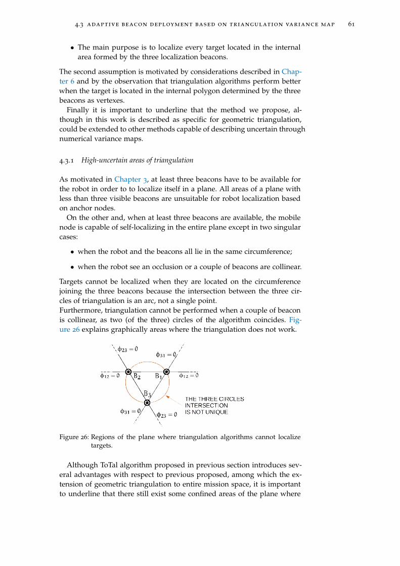
4.3 adaptive beacon deployment based on triangulation variance map 61
• The main purpose is to localize every target located in the internalarea formed by the three localization beacons.
The second assumption is motivated by considerations described in Chap-ter 6 and by the observation that triangulation algorithms perform betterwhen the target is located in the internal polygon determined by the threebeacons as vertexes.
Finally it is important to underline that the method we propose, al-though in this work is described as specific for geometric triangulation,could be extended to other methods capable of describing uncertain throughnumerical variance maps.
4.3.1 High-uncertain areas of triangulation
As motivated in Chapter 3, at least three beacons have to be available forthe robot in order to to localize itself in a plane. All areas of a plane withless than three visible beacons are unsuitable for robot localization basedon anchor nodes.
On the other and, when at least three beacons are available, the mobilenode is capable of self-localizing in the entire plane except in two singularcases:
• when the robot and the beacons all lie in the same circumference;
• when the robot see an occlusion or a couple of beacons are collinear.
Targets cannot be localized when they are located on the circumferencejoining the three beacons because the intersection between the three cir-cles of triangulation is an arc, not a single point.Furthermore, triangulation cannot be performed when a couple of beaconis collinear, as two (of the three) circles of the algorithm coincides. Fig-ure 26 explains graphically areas where the triangulation does not work.
Figure 26: Regions of the plane where triangulation algorithms cannot localizetargets.
Although ToTal algorithm proposed in previous section introduces sev-eral advantages with respect to previous proposed, among which the ex-tension of geometric triangulation to entire mission space, it is importantto underline that there still exist some confined areas of the plane where
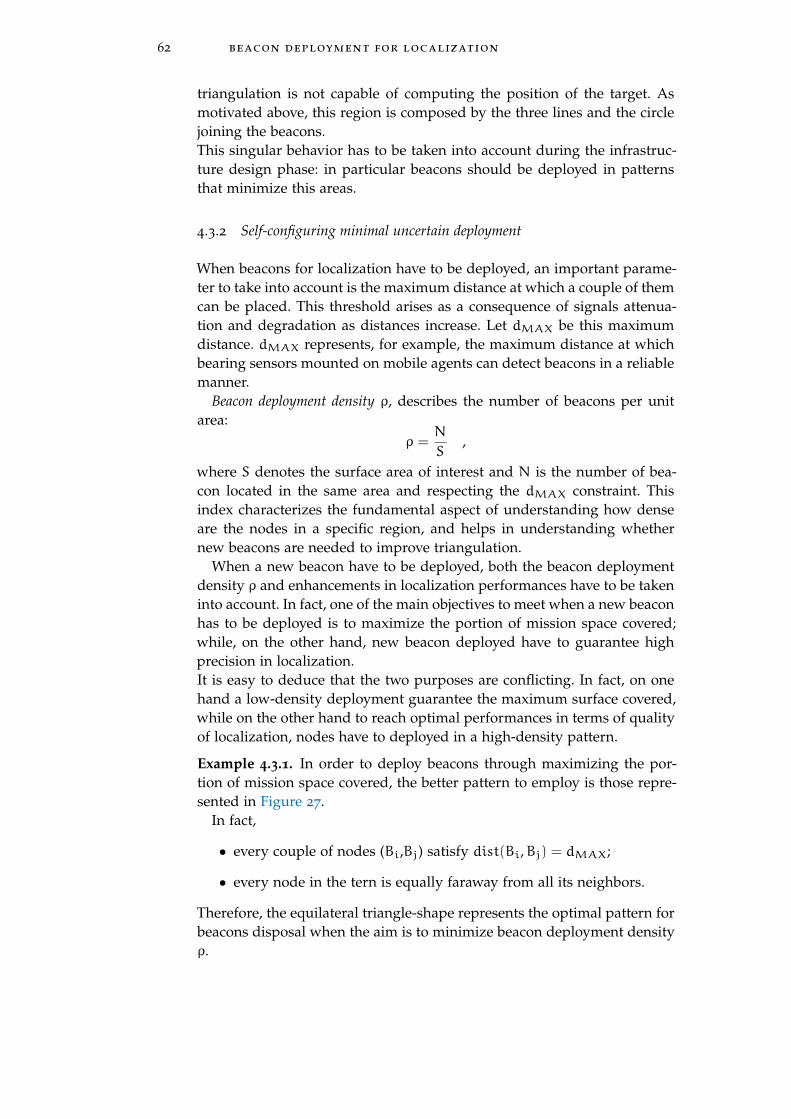
62 beacon deployment for localization
triangulation is not capable of computing the position of the target. Asmotivated above, this region is composed by the three lines and the circlejoining the beacons.This singular behavior has to be taken into account during the infrastruc-ture design phase: in particular beacons should be deployed in patternsthat minimize this areas.
4.3.2 Self-configuring minimal uncertain deployment
When beacons for localization have to be deployed, an important parame-ter to take into account is the maximum distance at which a couple of themcan be placed. This threshold arises as a consequence of signals attenua-tion and degradation as distances increase. Let dMAX be this maximumdistance. dMAX represents, for example, the maximum distance at whichbearing sensors mounted on mobile agents can detect beacons in a reliablemanner.
Beacon deployment density ρ, describes the number of beacons per unitarea:
ρ =N
S,
where S denotes the surface area of interest and N is the number of bea-con located in the same area and respecting the dMAX constraint. Thisindex characterizes the fundamental aspect of understanding how denseare the nodes in a specific region, and helps in understanding whethernew beacons are needed to improve triangulation.
When a new beacon have to be deployed, both the beacon deploymentdensity ρ and enhancements in localization performances have to be takeninto account. In fact, one of the main objectives to meet when a new beaconhas to be deployed is to maximize the portion of mission space covered;while, on the other hand, new beacon deployed have to guarantee highprecision in localization.It is easy to deduce that the two purposes are conflicting. In fact, on onehand a low-density deployment guarantee the maximum surface covered,while on the other hand to reach optimal performances in terms of qualityof localization, nodes have to deployed in a high-density pattern.
Example 4.3.1. In order to deploy beacons through maximizing the por-tion of mission space covered, the better pattern to employ is those repre-sented in Figure 27.
In fact,
• every couple of nodes (Bi,Bj) satisfy dist(Bi,Bj) = dMAX;
• every node in the tern is equally faraway from all its neighbors.
Therefore, the equilateral triangle-shape represents the optimal pattern forbeacons disposal when the aim is to minimize beacon deployment densityρ.
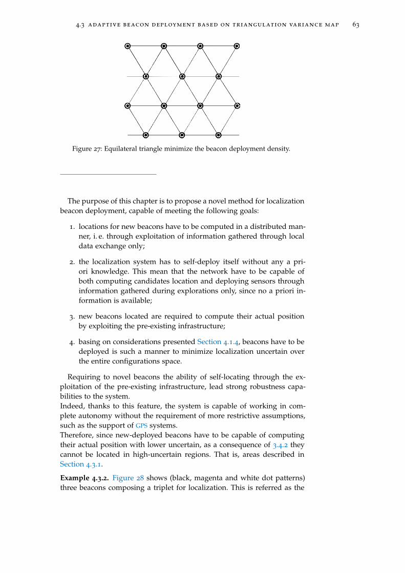
4.3 adaptive beacon deployment based on triangulation variance map 63
Figure 27: Equilateral triangle minimize the beacon deployment density.
The purpose of this chapter is to propose a novel method for localizationbeacon deployment, capable of meeting the following goals:
1. locations for new beacons have to be computed in a distributed man-ner, i. e. through exploitation of information gathered through localdata exchange only;
2. the localization system has to self-deploy itself without any a pri-ori knowledge. This mean that the network have to be capable ofboth computing candidates location and deploying sensors throughinformation gathered during explorations only, since no a priori in-formation is available;
3. new beacons located are required to compute their actual positionby exploiting the pre-existing infrastructure;
4. basing on considerations presented Section 4.1.4, beacons have to bedeployed is such a manner to minimize localization uncertain overthe entire configurations space.
Requiring to novel beacons the ability of self-locating through the ex-ploitation of the pre-existing infrastructure, lead strong robustness capa-bilities to the system.Indeed, thanks to this feature, the system is capable of working in com-plete autonomy without the requirement of more restrictive assumptions,such as the support of GPS systems.Therefore, since new-deployed beacons have to be capable of computingtheir actual position with lower uncertain, as a consequence of 3.4.2 theycannot be located in high-uncertain regions. That is, areas described inSection 4.3.1.
Example 4.3.2. Figure 28 shows (black, magenta and white dot patterns)three beacons composing a triplet for localization. This is referred as the
64 beacon deployment for localization
pre-existing localization infrastructure. The red dot represent the candi-date position for the new beacon in order to build an equilateral-triangleshape. The equilateral triangle show, in its internal, the variance map com-puted by the tern of pre-existing beacons.
Figure 28: The problem of locating a new beacon can be stated as a constrainedoptimization issue.
Therefore, in order to meet the overall objective, that is both minimizingbeacons density ρ and minimizing beacons location uncertain, a trade-offbetween the minimal-density and the minimal uncertain patterns have tobe chosen.The problem of locating a new beacon can then be formulated as a con-strained optimization of the variance map in areas of the plane that satisfythe dMAX constraint.
The novel method we propose is based on local cooperation betweenneighbor nodes, since each node requires only absolute positions of imme-diate neighbor.Each node can compute candidate positions for a new beacons accordingto following steps:
1. Exploiting locations of two neighbors and its relative uncertain, com-pute the variance map V(x,y) for the triplet of beacons;
2. Compute area of acceptable locations for the new node Ω, that is, lo-cation both respecting the dMAX constraint and avoiding beforehandtaken location. Notice that Ω ⊆ Ω;
3. Compute ultimate candidate locations for new nodes solving the fol-lowing constrained optimization problem:
minΩV(x,y) .

4.3 adaptive beacon deployment based on triangulation variance map 65
According to motivations just explained, in our algorithm we can iden-tify two main phases that lead to the design of the ultimate location fornew beacons:
1. design a candidate point according to density criteria;
2. adjust candidate location, reaching a trade-off, in order to obtainhigher accuracy.
Figure 29 explains the deployment process performed by a tern of pre-existing nodes.
Figure 29: Each beacon is responsible for the deployment of a couple of newnodes.
The figure emphasize the fact that each beacon is responsible for thedeployment of a couple of new nodes. Therefore each tern of pre-existingnodes can deploy three new beacons.
Another important aspect to underline, referring for instance to deploy-ment of node D, is that the design of its position is performed by bothnode A and node B. In absence of noise, designed locations coincides.However, in practical applications, this process can affected by some unat-tended aspects, among which:
• nodes belief about self location can be altered by noise;
• triangles formed by beacons can present shapes different form equi-lateral;
• communications can be ruined by noise;
• obstacles or errors during the deployment phase can alter the actualposition from the desired one.
This problem can be overcome through the introduction of a procedurebased on average consensus, operated by each node together immediateneighbor, in order to design location for beacons in common.Figure 30 schematizes the interaction, that produces ultimate location forthe beacon.
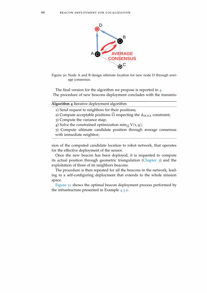
66 beacon deployment for localization
Figure 30: Node A and B design ultimate location for new node D through aver-age consensus.
The final version for the algorithm we propose is reported in 4.The procedure of new beacons deployment concludes with the transmis-
Algorithm 4 Iterative deployment algorithm
1) Send request to neighbors for their positions;2) Compute acceptable positions Ω respecting the dMAX constraint;3) Compute the variance map;4) Solve the constrained optimization minΩ V(x,y);5) Compute ultimate candidate position through average consensuswith immediate neighbor;
sion of the computed candidate location to robot network, that operatesfor the effective deployment of the sensor.
Once the new beacon has been deployed, it is requested to computeits actual position through geometric triangulation (Chapter 3) and theexploitation of three of its neighbors beacons.
The procedure is then repeated for all the beacons in the network, lead-ing to a self-configuring deployment that extends to the whole missionspace.
Figure 31 shows the optimal beacon deployment process performed bythe infrastructure presented in Example 4.3.2.
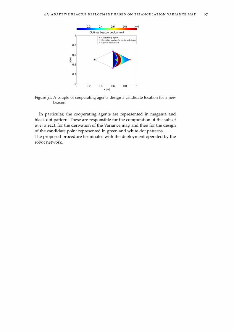
4.3 adaptive beacon deployment based on triangulation variance map 67
Figure 31: A couple of cooperating agents design a candidate location for a newbeacon.
In particular, the cooperating agents are represented in magenta andblack dot pattern. These are responsible for the computation of the subsetoverlineΩ, for the derivation of the Variance map and then for the designof the candidate point represented in green and white dot patterns.The proposed procedure terminates with the deployment operated by therobot network.

5C O V E R A G E C O N T R O L
In a sensor network, sensing devices can coordinate their actions throughwireless communication and aim at performing tasks in a shared manner.Indeed, capabilities of sensor networks are strictly linked to the coopera-tion between their nodes, in opposition with the approach used for cen-tralized controlled systems.The performance of a sensor network, in terms of its specific tasks, is sensi-tive to the location of its nodes in the mission space. This leads to the basicproblem of deploying sensors in order to meet the overall systems objec-tives, which is referred to as the coverage control or active sensing problem[5] [9].
In particular, sensors must be deployed so as to maximize the informa-tion extracted from the configurations space while maintaining acceptablelevels of communication and energy consumption. As the number of sen-sors deployed in the target area increase, then a more complex and effec-tive coverage method must be devised.
The static version of the solution to this problem involves positioningsensors without any further mobility; optimal location can be determinedby an off-line scheme which is akin to the widely studied facility locationproblem.The dynamic version allows the coordinated movement of sensors, whichmay adapt to changing conditions in the mission space, typically deploy-ing them into geographical areas with the highest information density.
Advantages characterizing the two methods can be combined via mixedsensor and robot networks, i. e. a network composed of both mobile andfixed agents. In fact services provided by the two types of cooperatingsystems are often complementary. This allow the cooperation to providenoticeable results in many fields of employment.
5.1 an overview on coverage control
Thanks to mobility capabilities provided by robotic agents, the dynamiccoverage control problem is in general managed by robots. However, it isimportant to underline that dynamic coverage control emerges as a resultof the cooperation between robot and sensor networks. In fact, while theactual dynamic coverage control is performed by robots, fixed sensors stillprovide anchor-based localization services. Moreover fixed beacons, whereneeded, can be employed in order to improve coverage performances. Thisleads to a mixed dynamic and static version for coverage control.
When we deal with unknown mission spaces, i. e. when we do not dis-pose of any information a priori, the initial requirement for agents is to op-erate in order to provide an initial model for the mission space. To achieve
69
70 coverage control
this goal, each robot needs to compute a path which allows itself to sensethe most dynamic areas as first, then to perform a comprehensive estima-tion for the remaining part. Such a path is referred to as an informativepath.
The key insight is to use a parameter function representing the rateof change of each point in the environment, while moving along a setof waypoints to optimize a cost function related to the informativenessof the path. The cost function attempts to place the path way-points atthe centroids of their Voronoi cells, while also making sure the waypointsare not too far from one other. The robot moves along the path, markingthe areas it observes as dynamic or static, and learning the environmentmodel.
The collection of the desired information is, in many cases, constrainedby the cost associated with obtaining it [26]. The cost of taking a measure-ment can be formulated in various manners. For many networks the mostsignificant may be the energy wasting for reaching the interested area ofthe mission space.
The objective is to determine an optimal control strategy to take theset of measurement, while simultaneously trying to minimize the cost oftaking those measurement, and this task must be fulfilled in a distributedway, that is, determining the optimal subdivision of explorations betweenthe team of robots.
5.1.1 Problem definition
The goal of guaranteeing full awareness coverage of the mission spaceemerges in many practical applications, where some regions are of muchmore importance with respect to the other regions in the mission domain.Consequently, one needs to discriminate these two classes of regions. Forexample, in an application where a mobile sensor network is employed tosurvey a nuclear power plant persistently, nuclear reactors must be cov-ered with full awareness while the the regions of less importance onlyneed to be revisited frequently. Coverage control can generally be classi-fied into:
• Static coverage control;
• Dynamic coverage control.
In static coverage control, the goal is to optimize the locations of fixedsensors in order to optimize the service provided by the entire network[10] [29]. Usually the static coverage problem can be referred as finding theminimum number of circles (circles represents the sensing area of agents)of radius R so that to completely cover the mission domain Ω. Usually thistypes of problems can be solved offline in a static manner.
When the mission space cannot be fully covered by any static configura-tion of the network, the problem of dynamic coverage arises; in this, eachpoint in the configuration domain is sampled by the mobile sensors until
5.1 an overview on coverage control 71
a prescribed coverage level is achieved [47] [51]. The movement of sensorsnot only impacts sensing performance, but it also influences other quality-of-service aspects in a sensor network, especially those related to wirelesscommunication.Because of limited on-board power and computational capacity of agents,a sensor network is not only required to sense but also to collect and trans-mit data as well in a reliable and optimal way. Particular attention has tobe given to the path that agents plans to get from a location to another, asenergy consumption constraints cold be limiting in many practical cases
For this reason, both sensing quality, communication performances andenergy-wasting need to be jointly considered when controlling the deploy-ment of sensors.
5.1.2 Previous work
The problem of optimizing sensor locations and sensor domains in fixedsensor networks has been extensively studied in the past: it can be consid-ered as an optimization problem [38], the solution is a Voronoi partitioning[12], where the optimal sensor domain is a Voronoi cell and the optimalsensor location is a centroid of a Voronoi cell.
On the other hand, mobile sensor coverage is relatively new in literatureand in [6] a survey of the most recent activities in control and design ofrobot static and dynamic sensor is presented. In [29], Li and Cassandrasconsider a probabilistic network model and a density function to repre-sent the frequency of random events taking place. The authors developan optimization problem that aims at maximizing coverage using sensorwith limited ranges, while minimizing communication cost. Starting withinitial sensor positions, authors developed a gradient-based algorithm tocoverage to a (local) solution to the optimization problem.
A similar goal is the focus in [52], where the notion of virtual forces isused to enhance the coverage of a sensor network given an arbitrary initialdeployment.
In [9] Cortes et al. address the same question, but in this case the trajec-tory converges to the centroid of a cell in a Voronoi partition of the searchdomain.
In [5] a coverage control scheme is developed which aims at the max-imization of target exposure in some surveillance applications, while in[52] a heuristic algorithm is applied to enhance the coverage of a sensornetwork. Much of the active sensing literature [37] also concentrates on theproblem of tracking specific targets using mobile sensors and the Kalmanfilter is extensively used to process observations and generate estimates.
5.1.3 Contribution
In this chapter, a distributed dynamic coverage control approach for coop-erative sensing devices is developed and presented. Motivated by Li and

72 coverage control
Cassandras in [29], the mission space has been modeled using a densityfunction representing the frequency that events take place.
We assume that a mobile sensor has a limited range which is defined bya probabilistic model. A deployment algorithm is applied at each mobilenode and it maximizes the joint detection probabilities of random events.We assume that the event density function is fixed and given. The exten-sion to density function time-variant does not require any modificationto the described approach as the adaptive relocation behavior naturallyfollows from the optimal coverage formulation.
In the work [29] presented by Li and Cassandras a novel method basedon an optimization that aims to converge to a local solution to the opti-mization problem is considered. The model proposed has been extendedin this work, in order to guarantee the obtainment of global optimal solu-tions.
The main contribution of this chapter is the development of a solutionfor the dynamic coverage control problem, through the maximization ofa cost functional. In particular the problem have been formulated by ex-ploiting optimal control theory. Moreover the proposed solution resultssuitable both for unknown environments and for common coverage con-trol problems, where the mission space is a priori known. The methodappears particularly interesting in order to perform an initial estimate ofthe state of the mission space.
Our approach is based on a distributed algorithm where each robotautonomously computes a Voronoi partitioning for its relative portion ofmission space. Each Voronoi cell is then exploited for estimating infor-mation enclosed in each partition. This type of partitioning helps in bothdetermining not yet visited areas and in defining their informativeness.The control scheme for mobile nodes, is then based on an optimizationstrategy, which aims to maximize information gathered.
5.1.4 Optimal coverage formulation
Let Ω ⊆ R2 models the mission space, over which there exists an eventdensity function
R(x), x ∈ Ω (31)
that models the frequency or density that a specific random event takesplace. Being a density function, R(x) satisfies:
• R(x) > 0 ∀x ∈ Ω;
•∫Ω R(x) = 1.
R(x) can, for instance, model the frequency that a certain type of eventappears at x, or it could be the probability that a certain measured valueexceeds a specific threshold at x.
In the mission space Ω, there are N mobile sensors located at s =
s1, . . . , sN, si ∈ R2 i = 1, . . . ,N .

5.2 distributed solution to the optimal coverage problem 73
When an event occurs at point x, it emits a signal and this is observedby a sensor at location si. The received signal strength generally decayswith ||x − si||, i. e. the distance between the source and the sensor. Thisdegradation can be modeled by a monotonically decreasing diffentiablefunction pi(x), which expresses the probability that sensor i detects theevent occurring at x.
For instance, a sensor model with a simply form may be:
pi(x) = p0ie−λi||x−si||
that expresses the idea that the detection probability declines exponen-tially with distance.p0i and λi are determined by physical characteristics of the sensor. Theoptimal coverage problem can be formulated as maximizing the proba-bility that events are detected. When an event takes place at x, and it isobserved by the sensors, the joint probability that this event is detectedcan be expressed by:
P(x, s) = 1−N∏i=1
[1− pi(x)] (32)
where we have assumed that sensors take observations independently.
Definition 5.1. The optimal coverage problem can be formulated as an op-timization problem that maximizes the expected event detection frequencyby the sensors, over the entire mission space Ω:
maxs
∫Ω
R(x)P(x, s)dx := max F(s) (33)
In (33) controllable variables are the locations of mobile sensors s. The re-sult of optimization (33), computed with respect to si, gives new positionsfor mobile robots si, i = 1, . . . ,N that maximize the number of detectedevents.
In general, this kind of problem can be solved by applying a non-linearoptimizer with an algorithm which can evaluate integrals numerically: insuch a case, a centralized controller with intensive computational capacityis required.
5.2 distributed solution to the optimal coverage problem
While in general terms, the solution to the optimal coverage problem isprovided through centralized systems due to both the requirement ofglobal knowledge of robots positions and the computational complexityrequired, this section proposes a distributed method to solve the optimalcoverage problem.
Taking partial derivatives with respect to si, i = 1, . . . ,N, in order tosolve Equation 33, we have:
∂F(s)
∂si=
∫Ω
R(x)∂P(x, s)∂si
dx . (34)
74 coverage control
Using Equation 32, the partial derivative (34) can be rewritten as:
∂F(s)
∂si=
∫Ω
R(x)
N∏k=1,k6=i
[1− pk(x)]dpi(x)
dsi(x)dx . (35)
In general, (35) cannot be computed directly by mobile sensors, sinceit requires global information such as the value of R(x) over the wholemission space and the exact location of all other sensors in the network. Inaddition, the evaluation of integrals remains a significant task for cheapestsensors.
If partial derivative might be evaluated locally by each mobile sensor,then a gradient method could be applied which directs agents towardslocations that maximize F(s).
In order to render distributed the optimal coverage problem, mobilenodes must be capable of computing the optimization (33) with the avail-ability of local knowledge only. This mean that only local exchange ofinformation between neighbor nodes, is needed.
Basing on the physical observation that when di(x) >> 1, pi(x) ' 0, weassume:
pi(x) = 0, ∀x s.t. ||x− si|| > D (36)
where D denotes the sensing radius. Thus ||x− si|| defines the region ofcoverage of sensor i. Since pi(x) = 0 for all x 6∈ Ωi, Ω can be replaced byΩi in Equation 35, where Ωi = x : ||x− si|| < D.Moreover, indexes taken by variable k in the product can be limited insuch a way to consider only nodes in the neighboring Bi, i. e. nodes thathave their detectable area in common with the detect area of node i: Bi =k : ||si − sk|| < 2D,k = 1, . . . ,N,k 6= i.Thus, Equation 35 can be rewritten as:
∂F(s)
∂si=
∫Ωi
R(x)∏k∈Bi
[1− pk(x)]dpi(x)
dsi(x)dx . (37)
In conclusion we have obtained a useful and simply way to solve in adistributed manner the problem of the optimal coverage by introducing asimply simplification that takes into account the reduced sensing capaci-ties of real sensors.
As a consequence of the local knowledge only required to solve the max-imization, in general Equation 37 provides solutions for local maximumfor the function R(x).
In order to reduce computation costs in making Equation 37, the integralevaluation can be discretized [29]. This type of solution is often taken intoaccount in many practical cases and could be evaluated in future works.
Example 5.2.1. Figure 32 shows simulation results about a network com-posed of a couple of mobile agents exploiting a control strategy accordingto Equation 37. Events density R(x) has been modeled with three peakslocated in (0.4, 0.5), (0.8, 0.2) and (0.8, 0.8).
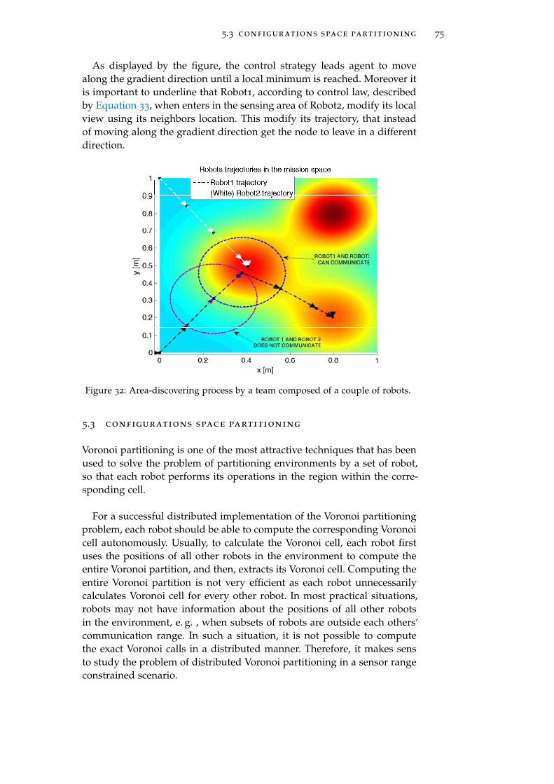
5.3 configurations space partitioning 75
As displayed by the figure, the control strategy leads agent to movealong the gradient direction until a local minimum is reached. Moreover itis important to underline that Robot1, according to control law, describedby Equation 33, when enters in the sensing area of Robot2, modify its localview using its neighbors location. This modify its trajectory, that insteadof moving along the gradient direction get the node to leave in a differentdirection.
Figure 32: Area-discovering process by a team composed of a couple of robots.
5.3 configurations space partitioning
Voronoi partitioning is one of the most attractive techniques that has beenused to solve the problem of partitioning environments by a set of robot,so that each robot performs its operations in the region within the corre-sponding cell.
For a successful distributed implementation of the Voronoi partitioningproblem, each robot should be able to compute the corresponding Voronoicell autonomously. Usually, to calculate the Voronoi cell, each robot firstuses the positions of all other robots in the environment to compute theentire Voronoi partition, and then, extracts its Voronoi cell. Computing theentire Voronoi partition is not very efficient as each robot unnecessarilycalculates Voronoi cell for every other robot. In most practical situations,robots may not have information about the positions of all other robotsin the environment, e. g. , when subsets of robots are outside each others’communication range. In such a situation, it is not possible to computethe exact Voronoi calls in a distributed manner. Therefore, it makes sensto study the problem of distributed Voronoi partitioning in a sensor rangeconstrained scenario.
76 coverage control
5.3.1 Problem formulation
Considering a team of robotic agents, the problem of partitioning the con-figurations space consists in dividing it into a number of regions, eachof them could then be assigned to single agents. The approach exploitedcould be static or dynamic.When a static approach is used, the partitioning is static through time andboth sizes and locations of the partitions are in general fixed. This perspec-tive is easier to implement as it can be studied during the setup phase ofthe network.On the other hand, when a dynamic approach is exploited, partitions areperiodically re-updated in terms of their sizes and locations, following theupdates recorded by measuring and needs of the entire network.
Assuming to dispose of an initial sets of points, representing the sets of"centers" of the partitions involved we can proceed as follow. Let Ω be anopen convex set representing the mission space, Ω ∈ R2, and let Ω theinternal set of Ω; we can define:
Definition 5.2. The set ViNi=1 is called a tessellation of Ω if:
• Vi ∩ Vj =6 0 fori 6= j;
• ∪Ni=1Vi = Ω
Definition 5.3. Given a set of points ziNi1 , belonging to Ω, the Voronoiregion Vi corresponding to the point zi is defined by:
Vi = x ∈ Ω : ||x − zi|| < ||x − zj|| for j = 1, . . . ,N, j 6= i (38)
where || · || denotes the Euclidean norm on R2
The points ziNi=1 are called generators.The set ViNi=1 is a Voronoi tessellation or Voronoi diagram of Ω, and each Viis referred to as the Voronoi region corresponding to zi.
Given a region Vi ∈ R2 and a density function ρ defined in Vi, the masscentroids z∗ of Vi is defined by:
z∗ =∫Vixρ(x)dx∫
Viρ(x)dx
(39)
Let f be an increasing function of distances between elements of Ωf : R+ → R+ and let φ be a weight function φ : Ω→ R+ that gives a dis-tinct priority to various areas of the mission space. Function f(·), could forexample represent the energy consumption of the mobile node in movingin the mission space, while the function φ(·) can be chosen proportionalto the objective function, in such case a greater number of sensors wouldbe deployed in regions of major interests.
The optimal partitioning problem, that minimizes distances between ac-tual locations of every nodes and considering the weight function Φ canbe solved by minimizing the function:
H :=
N∑i=1
∫Vi
f(||si − x||)φ(s)ds (40)

5.3 configurations space partitioning 77
Figure 33: On the left, the Voronoi regions corresponding to 10 randomly selectedpoints in a square, using a uniform density function. The dots are theVoronoi generators (38) and the circles are the centroids (39) of thecorresponding Voronoi regions . On the right, a 10 point centroidalVoronoi tessellation. In this case, the dots are simultaneously the gen-erators for the Voronoi tessellation and the centroids of the Voronoiregions.
where x ∈ Ω.
5.3.2 Voronoi partitioning
Proposition 5.3.1. Optimal regions, obtained by minimizing Equation 40 cor-responds to the Voronoi regions, weighted by the cost function φ(s) and aredefined as follow:
Vi := s ∈ Ω : ||q − si|| 6 ||q − si||,∀i 6= j
in particular, the weight function assumes the minimum value:
HVOR =
∫Ω
mini∈1,...,N
f(||si − q||)φ(q)dq
In the following, we assume the specific form for the function f(·):
f(||si − q||) := ||si − q||2 .
GivenN points zi, i = 1, . . . ,N ,representing the Voronoi generators (38),we can define their associated Voronoi regions Vi, i = 1, . . . ,N. Further-more, given the regions Vi, i = . . . ,N, we can define their mass centroidsz∗i , i = 1, . . . ,N using Equation 39.
On the other hand, we can consider the following problem: given a re-gion Ω ⊆ R2, a positive integer N and a density function ρ defined forevery x in Ω; find N points zi ∈ Ω and N regions Vi that tessellate Ω,such that for each i, Vi is the Voronoi region for zi and zi is the masscentroid of Vi.
The described problem, corresponds to many practical cases in whichrobots are initially located in the same initial positions, or when we areinterested in finding an optimal tessellation of the configurations space Ωwithout considering the initial positions of mobile nodes.
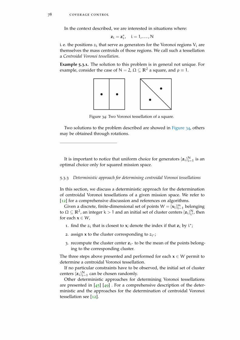
78 coverage control
In the context described, we are interested in situations where:
zi = z∗i , i = 1, . . . ,N
i. e. the positions zi that serve as generators for the Voronoi regions Vi arethemselves the mass centroids of those regions. We call such a tessellationa Centroidal Voronoi tessellation.
Example 5.3.1. The solution to this problem is in general not unique. Forexample, consider the case of N = 2, Ω ⊆ R2 a square, and ρ ≡ 1.
Figure 34: Two Voronoi tessellation of a square.
Two solutions to the problem described are showed in Figure 34, othersmay be obtained through rotations.
It is important to notice that uniform choice for generators ziNi=1 is anoptimal choice only for squared mission space.
5.3.3 Deterministic approach for determining centroidal Voronoi tessellations
In this section, we discuss a deterministic approach for the determinationof centroidal Voronoi tessellations of a given mission space. We refer to[12] for a comprehensive discussion and references on algorithms.
Given a discrete, finite-dimensional set of points W = xlml=1 belongingto Ω ⊆ R2, an integer k > 1 and an initial set of cluster centers ziNi1 , thenfor each x ∈W,
1. find the zi that is closest to x; denote the index if that zi by i∗;
2. assign x to the cluster corresponding to zi∗ ;
3. recompute the cluster center zi∗ to be the mean of the points belong-ing to the corresponding cluster.
The three steps above presented and performed for each x ∈ W permit todetermine a centroidal Voronoi tessellation.
If no particular constraints have to be observed, the initial set of clustercenters ziNi=1 can be chosen randomly.
Other deterministic approaches for determining Voronoi tessellationsare presented in [45] [49] . For a comprehensive description of the deter-ministic and the approaches for the determination of centroidal Voronoitessellation see [12].
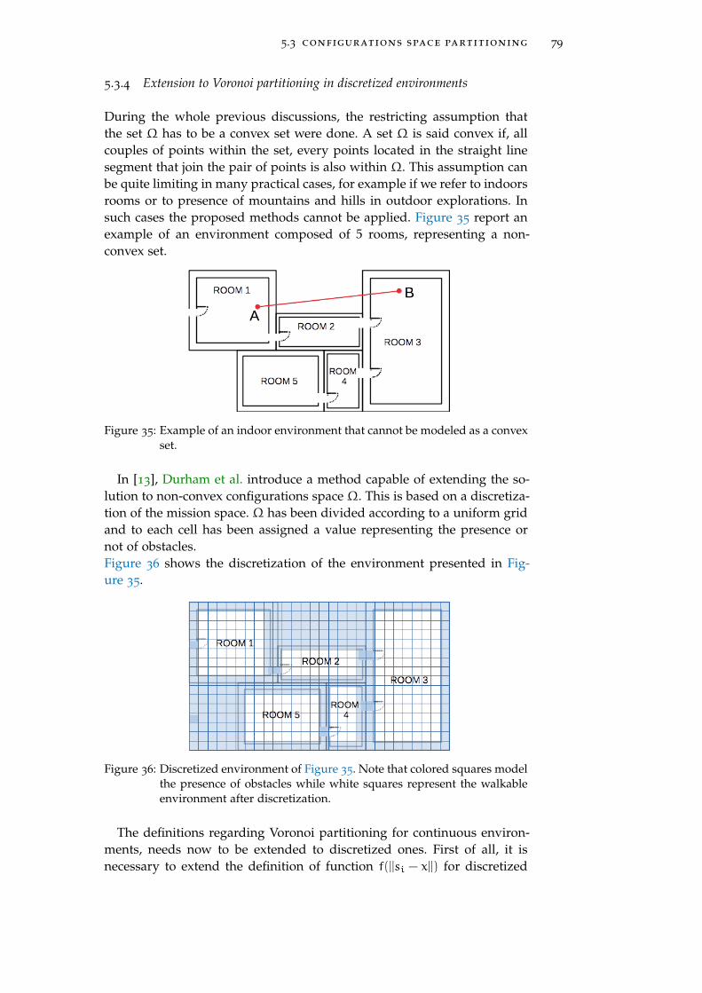
5.3 configurations space partitioning 79
5.3.4 Extension to Voronoi partitioning in discretized environments
During the whole previous discussions, the restricting assumption thatthe set Ω has to be a convex set were done. A set Ω is said convex if, allcouples of points within the set, every points located in the straight linesegment that join the pair of points is also within Ω. This assumption canbe quite limiting in many practical cases, for example if we refer to indoorsrooms or to presence of mountains and hills in outdoor explorations. Insuch cases the proposed methods cannot be applied. Figure 35 report anexample of an environment composed of 5 rooms, representing a non-convex set.
Figure 35: Example of an indoor environment that cannot be modeled as a convexset.
In [13], Durham et al. introduce a method capable of extending the so-lution to non-convex configurations space Ω. This is based on a discretiza-tion of the mission space. Ω has been divided according to a uniform gridand to each cell has been assigned a value representing the presence ornot of obstacles.Figure 36 shows the discretization of the environment presented in Fig-ure 35.
Figure 36: Discretized environment of Figure 35. Note that colored squares modelthe presence of obstacles while white squares represent the walkableenvironment after discretization.
The definitions regarding Voronoi partitioning for continuous environ-ments, needs now to be extended to discretized ones. First of all, it isnecessary to extend the definition of function f(||si − x||) for discretized
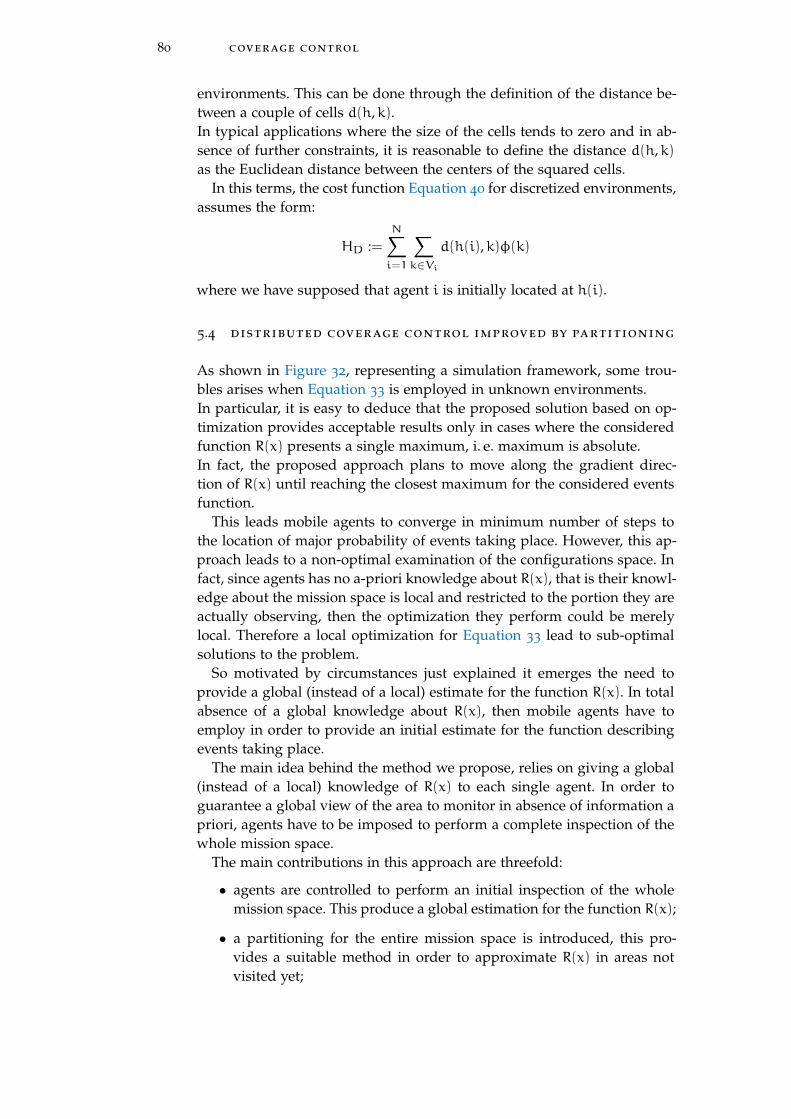
80 coverage control
environments. This can be done through the definition of the distance be-tween a couple of cells d(h,k).In typical applications where the size of the cells tends to zero and in ab-sence of further constraints, it is reasonable to define the distance d(h,k)as the Euclidean distance between the centers of the squared cells.
In this terms, the cost function Equation 40 for discretized environments,assumes the form:
HD :=
N∑i=1
∑k∈Vi
d(h(i),k)φ(k)
where we have supposed that agent i is initially located at h(i).
5.4 distributed coverage control improved by partitioning
As shown in Figure 32, representing a simulation framework, some trou-bles arises when Equation 33 is employed in unknown environments.In particular, it is easy to deduce that the proposed solution based on op-timization provides acceptable results only in cases where the consideredfunction R(x) presents a single maximum, i. e. maximum is absolute.In fact, the proposed approach plans to move along the gradient direc-tion of R(x) until reaching the closest maximum for the considered eventsfunction.
This leads mobile agents to converge in minimum number of steps tothe location of major probability of events taking place. However, this ap-proach leads to a non-optimal examination of the configurations space. Infact, since agents has no a-priori knowledge about R(x), that is their knowl-edge about the mission space is local and restricted to the portion they areactually observing, then the optimization they perform could be merelylocal. Therefore a local optimization for Equation 33 lead to sub-optimalsolutions to the problem.
So motivated by circumstances just explained it emerges the need toprovide a global (instead of a local) estimate for the function R(x). In totalabsence of a global knowledge about R(x), then mobile agents have toemploy in order to provide an initial estimate for the function describingevents taking place.
The main idea behind the method we propose, relies on giving a global(instead of a local) knowledge of R(x) to each single agent. In order toguarantee a global view of the area to monitor in absence of information apriori, agents have to be imposed to perform a complete inspection of thewhole mission space.
The main contributions in this approach are threefold:
• agents are controlled to perform an initial inspection of the wholemission space. This produce a global estimation for the function R(x);
• a partitioning for the entire mission space is introduced, this pro-vides a suitable method in order to approximate R(x) in areas notvisited yet;
5.4 distributed coverage control improved by partitioning 81
• interest in non-visited partitions is updated over time.
Moreover, the following assumptions are considered:
• although an accurate model for the mission space requires the func-tion R(x) changing over time, i. e. R(x) = R(x, t), it reasonable toassume function R(x, t) slowly changing over time; this justify thefollowing:
• when a partition get visited at time t∗ by one agent of the network,then the agent has a detailed knowledge of that area, Hence in R(x, t)the dependence on t disappear.
Let us denote by Pv(x, t− k) the probability that point x have been vis-ited by almost one agent of the network during last (t− k) steps. Let theset ViNi=1 be a tessellation of Ω.
The optimal coverage problem presented in Section 5.1.4 can be ex-tended, leading agents to build a global knowledge of the function R(x, t)for each agent, by enhancing the weight function F(s) in Equation 33 asdescribed by the following:
F1(s) =
∫Ωi
R(x)Pi(x, s)dx+N∑i=1
∫Vi
(1− Pv(x, t− k))dx . (41)
Notice that (1− Pv(x, t− k)) represents the probability that x has not beenvisited during last t− k steps by any agent of the network.The additional term introduced, with respect to Equation 33, induces anincrement in the function F(s) in correspondence of partitions that havea lower probability of being already visited by any agent. The relativeincrease of F(s) in correspondence of these points, can be interpreted as anenhancement in the interest that the network has in visiting this points, asthey have never been visited before.
It is important to underline that the tessellation ViNi=1 has to be shared
among all the agents composing the network.In order to insert dynamics induced by non-visited areas, Equation 41
can be improved introducing the grows in interest in non-visited partitions:
F2(s, t) =∫Ωi
R(x)Pi(x, s)dx+N∑i=1
∫Vi
[1−Pv(x, t− k)]ρ(x, t− k)dx . (42)
where ρ(x, t− k) is a monotonic increasing function of time t.The function [1−Pv(x, t−k)]ρ(x, t−k) indicates the probability that x havenot been visited during the last (t− k) steps, and this should a monotonicincreasing function over time t to produce growth in interest in non-visitedcells.
Example 5.4.1. For instance, typical models for the probability Pv(x) inregular (squared) mission spaces are:
Pv(x) ∼ N(µ,σ) .
82 coverage control
In fact, we can suppose that central points of the mission space are exam-ined more frequently, while peripheral areas are less frequently visited.
In addition, more sophisticated agents, can be equipped with memo-ries containing previously visited partitions. In this type of systems, thefunction Pv(x) degenerates to the deterministic case.
This kind of approach is implemented and described in detail simula-tion results in Chapter 6
Proposition 5.4.1. Given a robot network operating in Ω, comprehending onerobotic agent implementing weight function described by (47).Let R(x) be the probability density function describing frequencies at which eventstakes place in Ω and let ρ(t) be a monotonic increasing function of t in [0, t].Let the set ViNi=1 be a tessellation of Ω.
Then the whole mission space is being visited in a time t∗ such that:
ρ(t∗) = N · R|Ω|
|Vi|. (43)
where R = maxx R(x) and | · | denotes the area of the polygon described by itsargument.
Proof. In order to fix ideas, let us set k = 0, i. e. we consider the entire timeframe [0, t]. The proposition can be demonstrated, by showing that holds:∫
Ωi
R(x)Pi(x, s)dx <∫Vi
[1− Pv(x, t)]ρ(x, t)dx·
where Vi represent the most interesting partition of the mission space.Since R(x) is a probability density function,∫
Ω
R(x)dx = 1
then it is also a limited function i. e.
∃R R(x) < R .
Since P(x, s) represents a probability, i. e. P(x, s) ∈ [0, 1] we can considerthe following inclusions:∫
Ωi
R(x)Pi(x, s)dx 6 R∫Ωi
1dx 6 R|Ω| (44)
where |Ω| represent the area of the polygon described by Ω.Let ρ(x, t) be a constant function over the entire partition Vi, i. e. :
ρ(x, t) = ρ(t)
5.4 distributed coverage control improved by partitioning 83
In a similar manner, for all the partitions Vj that have not been visited yet,we can write:∫
Vi
[1− Pv(x, t)]ρ(x, t)dx >∫Vi
1dx · ρ(t)· (45)
since:
• 1− Pv(x, t) = 1, since partition i have not been visited;
• the function ρ(t) can be brought outside the sign of integral as itdoes not depend on x.
Denoting∫Vi1dx as |Vi|, and combining Equation 44 and Equation 45,
together with Equation 47 we obtain:
R|Ω| < |Vi| · ρ(t)·
Assuming ρ(t) be a monotonic increasing function of t, we can state thatpartition Vi will surely be visited when
ρ(t) >R|Ω|
|Vi|(46)
In addition, it is important to underline that condition (43) guaranteesthe visit of partition i as ρ(t) is a monotonic increasing function.
Starting from this assumption, each mobile agent can then move to otherpartitions in order to create a global estimate of the whole space.
5.4.1 Adding distances cost
Although Equation 42 arises as a robust and effective technique, capable ofexploring the whole configurations space in a upper-bounded time, someimprovements can be introduced in order to improve energy consumption.In fact, motivated by simulations results proposed in Chapter 6, it is easyto imagine that trajectories performed by the agents are not optimal, sincethe weight function considers only informativeness of partitions, whileenergy consumption needed to reach the partition is neglected.
More efficient results in terms of distance traveled by agents, can beobtained by weighting the additional term proposed in Equation 42 withthe distance that the agent needs to travel in order to reach the partition ofinterest. In particular, the Euclidean distance ||zi− zj|| between the centroidof the actual Voronoi cell and the centroid of the partition of interest isused.
Therefore, the weight function considered is:
F3(s, t) =∫Ωi
R(x)Pi(x, s)dx+
+
N∑i=1
∫Vi
[1− Pv(x, t− k)]ρ(x, t− k)dx · ||zi − zj||−1i 6=j (47)
84 coverage control
where zj denotes the centroid of the currently partition in which the agentresides, and zi indicates the generic centroid of partition i.
5.4.2 Iterative update of mission space model
Control strategies proposed in previous sections provide suitable and ef-fective method in order to
• perform an initial estimation for the function R(x), when configura-tions spaces are unknown;
• perform optimal coverage control, when R(x) is exactly known.
Indeed, once an initial estimation for R(x) is made, then control strategydefined by (33) provides a robust solution to the coverage control problem.
Therefore we deal with two different control strategies, both based onoptimization, the former capable of estimating R(x) while the other capa-ble of performing optimal coverage control. Our purpose for this section,is to study and present how these two methods can be combined in orderto provide a system able to self-update and to provide optimal coveragecontrol in time-variant mission spaces.
When the actual function R0(x) = R0(x, t) i. e. the function that describeactual frequency of events taking place is variable over time, we are in-terested in providing a strategy that continuously update our estimatedmodel R(x, t), in order to get an updated model describing the missionspace.It is important to underline that in this process of initialization for R(x, t),areas rapidly changing over time i. e. areas described by peaks for R(x, t)requires to be visited more frequently.
In the following, we propose an iterative method capable of fulfillingcontrol objectives just explained, through combining optimal control de-scribed weight functions (33) and (42). Our method, is based on an iterativeapplication of the two control laws, as described in detail by the followingflux diagram:
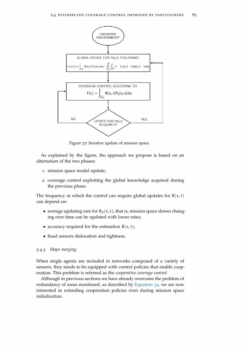
5.4 distributed coverage control improved by partitioning 85
Figure 37: Iterative update of mission space.
As explained by the figure, the approach we propose is based on analternation of the two phases:
1. mission space model update;
2. coverage control exploiting the global knowledge acquired duringthe previous phase.
The frequency at which the control can require global updates for R(x, t)can depend on:
• average updating rare for R0(x, t), that is, mission space slower chang-ing over time can be updated with lower rates;
• accuracy required for the estimation R(x, t);
• fixed sensors dislocation and tightness.
5.4.3 Maps merging
When single agents are included in networks composed of a variety ofsensors, they needs to be equipped with control policies that enable coop-eration. This problem is referred as the cooperative coverage control.
Although in previous sections we have already overcome the problem ofredundancy of areas monitored, as described by Equation 32, we are nowinterested in extending cooperation policies even during mission spaceinitialization.

86 coverage control
In fact, according to control policies described in previous sections, agentsperform initial estimation R(x) according to Equation 42 in an autonomousmanner, that is, without exploiting cooperation with neighbors.
In this context, cooperation policies forces agents to combine their knowl-edge about the environment that has been acquired during the initializa-tion process, whenever an encounter occur.
This approach can be explained with the aid of the following figure:
Figure 38: Single agents knowledge are combined, whenever an encounter occur.
where, as a consequence of the meeting between Robot1 and Robot2,their local map have been combined in order to build an overall knowledgefor the environment. Subsequently both agent dispose of the combinedknowledge of the configurations space.
5.5 beacon placement for coverage control
In dynamic coverage control, agents are capable of moving in order to in-crease the area covered with time, until every point in the given area hasbeen covered with some prescribed coverage level. Thanks to mobility ofagents employed, the network can adapt for changing conditions in themission space, and enable the network to monitor widely extended areas,even when employing a reduced number of sensors.
On the other hand, the static approach to coverage control involves po-sitioning sensors without any further mobility. Thus, Static coverage controldeals with achieving an arrangement for agent that minimizes the proba-bility of undetected events. The sensors or agents determine optimal posi-tions based on gradient climbing methods, until the optimal configurationis reached. The optimal configuration maximize the collective reward func-tion.

5.5 beacon placement for coverage control 87
Advantages introduced by Static coverage control, athwart dynamic ap-proach are twofold:
• persistent sensing of interested areas;
• higher coverage levels;
These aspect cannot be in general guaranteed by the dynamic version,since nodes are required to travel across the configurations space in orderto cover larger extension areas. On the other hand, in such cases in whichR(x, t) is highly changing over time, fixed sensors become unnecessarysince their position cannot be determined in optimal manner.
Motivations just explained, justify a mixed coverage control, that is, theexploitation of both fixed and robotic sensor in order to perform a robustand reliable coverage control when R(x, t) ≈ R(x).
In the following, our purposes are twofold:
• providing a given covered threshold for areas with the highest infor-mation density;
• maintaining complete covering of the remaining areas of the missionspace.
5.5.1 Static sensor coverage model
Assume the network is a squared sensor field Ω and k sensors have to bedeployed. Each sensor has a detection range rs, and sensor si is deployedat (xi,yi). For any point P at (x,y), we denote the Euclidean distancebetween si and P as:
d(si,P) = (xi − x)2(yi − y)
2 . (48)
A typical sensor model expresses the coverage Cxy(si) of the sensor sias:
Cxy(si) =
1 if d(si,p) < rs
0 otherwise(49)
for all P ∈ Ω. It assumes that sensor readings have no associated uncer-tainty in reality, and sensor detection are imprecise.
When the coverage Cxy(si) needs to be expressed in probabilistic terms,hence a precise detection model is introduced:
Cxy(si) =
0 if d(si,P) > r+ rl
e−λαβ
if r− rl < d(si,P) < r+ rl
1 if d(si,P) 6 r− rl
(50)
where α = d(si,P) − (r− rl) and rl (rl < r) is a measure of uncertaintyin the sensor detection, α and β are parameters that measure detection

88 coverage control
probability when a target is at distance greater than rl but within maxi-mum from the sensor. This model reflects the behavior of range sensingdevices such as infrared and ultrasound sensors. Typical values for param-eters involved are: r = 10, rl = 5, β = 0.5 and λ = 0.5.
Figure 39: Optimal hexagon-based sensor distribution.
The choice for parameter rl lead to two different behaviors:
• when rl ' 0 i. e. rl can be neglected, we are using the binary sensordetection model, attempting to prevent the detection region of twosensors from overlapping. This optimal distribution of sensor nodesis illustrated in Figure 39.
• if rl > 0 the probabilistic sensor detection is used. Due to uncertaintyin sensor detection responses, grid points are not uniformly coveredwith the same probability. Some grid points will have lower coveragerate if they are covered only by one sensor and far from other sensors.In this case, it is necessary to overlap the sensor detection area tocompensate for the low detection probability.
The probability of the point (x,y) being covered by a couple of sensorssi, sj is denoted as,
Cxy(si, sj) = 1− (1−Cxy(si))(1−Cxy(sj)) .
Definition 5.4. Let Cth be the desired coverage threshold for all gridpoints. The problem of maintaining a given covered threshold can be for-mulated as finding locations for sensing devices si, sj such that, for allpoints (x,y) in the mission space:
minx,y
Cxy(si, sj) > Cth . (51)
It can also be extended to a region which is overlapped by a set of ksensors. That is s1, s2, . . . , sk. The coverage in this case is given by:
Cxy(k) = 1−∏
j=1,...,k
(1−Cxy(sj)) (52)

5.5 beacon placement for coverage control 89
5.5.2 Coverage control through mixed robot and sensor networks
The method we propose is based on a mixed network, i. e. on a group com-posed of both fixed and robotic agents. In particular, our control schemeinvolves:
• fixed sensors for monitoring areas with the highest information den-sity;
• robotic agents for monitoring remaining areas of the mission space.
Thanks to the cooperation between the dynamic and Static coveragecontrol schemes, our method is able to guarantee a persistent sensing inhighly informative areas, while the remaining areas of mission space con-tinue in being completely covered thanks to mobile agents. Let RMIN bea threshold that discriminates between highly an lower informative areas,that is:
• if R(x) > RMIN ⇒ x is considered a highly-informative point
• if R(x) < RMIN ⇒ x is considered a lower-informative point
and letR(x) := x : R(x) > RMIN
the region containing highly-informative points.In the following, it is reasonable to assume the following:
1. robotic nodes are capable of deploying fixed sensors in the missionspace.
It is moreover important to recall the previously-stated assumptionR(x, t) ≈ R(x). This enables to state that function R(x), and in particular itspeaks, are almost not varying over time. This assumption is fundamentalin order to compute fixed sensors optimal locations; in fact this kind ofagents are capable of guaranteeing higher coverage levels but their do notprovide flexibility in terms of mobility.
Exploiting global knowledge of the mission space own by robotic agent,the design of candidate location for fixed sensors can be performed as aglobal optimization problem. Therefore mobile agents can compute loca-tions for fixed sensors nodes through:
si = x|maxxR(x)
mobile agents are then capable of deploying fixed sensors directly thanksto assumption (2).
This approach arises as a suitable method capable of monitoring with ahigh update rate areas where events takes place frequently, while the re-maining parts of the configurations space continues to maintain acceptablelevels of coverage thanks to mobile agents.
For a detailed description on persistent coverage control, please refer to[9] and [20].


Part III
S I M U L AT I O N R E S U LT S
Simulations results allow to assess novel solutions proposedin the theoretical previous chapters. Methods described in pre-vious chapters to improve network task quality through inter-play between sensor and robotic network are validated and dis-cussed through Matlab simulation software.

6S I M U L AT I O N R E S U LT S I N M AT L A B
This chapter presents numerical simulations performed in order to vali-date theoretical approaches described in previous chapters. The simula-tion setup comprises a unit square mission space (1m x 1m), with threefixed beacons employed to perform localization. Robotic agents are repre-sented with colored triangles. Triangular-shape displays both position andorientation of the agent. Beacons are in general represented by black andwhite dot patterns.
Simulations are organized in sections, each of them comprehend resultsregarding previous chapters; in particular:
• Section 6.1 presents simulations results regarding Chapter 3;
• Section 6.2 presents simulations results regarding Chapter 4;
• Section 6.3 presents simulations results regarding Chapter 5;
6.1 localization
In the former part of this Section, odometric techniques are described andanalyzed in terms of quality of target estimated position, when noise af-fects sensors readings.In the second part, closed-form expressions for variance of computed lo-cations are exploited in order to graphically derive the uncertain behavioras function of target’s location; results obtained are then discussed andcompared in terms of both localization error and variance of estimatedposition. The part moreover introduce a comparison between methods intypical agent trajectories.The third part of the Section concludes describing performances of statisti-cal filtering in simulation results. The implementation of the Kalman filteris discussed in detail and design choices are motivated and discussed.
6.1.1 Dead reckoning
Dead-reckoning is the most widely odometry-based method employed fordetermining position and orientation of a specific target. In many practicalapplications dead-reckoning provides easily and accessible real-time posi-tioning information. In general, the frequency at which the measurementsand the algorithm have to be performed depends to a large degree on therequested accuracy for the system.
Dead-reckoning is a relative positioning method, and it consists of evalu-ating the position of a mobile robot by using velocity and angles measuredby encoders attached to the robot’s wheels. This method estimates relative
93
94 simulation results in matlab
position of the target by exploiting information about its initial locationand then integrating measured gathered by sensors. The main advantagesare that it is simple, low-cost and has an easier time in estimating the po-sition in real time, compared to absolute positioning methods.However, since it is based on the odometric information arising fromwheels, this kind of methods are subject to major accumulation of errorscaused by wheel slippage, mechanical tolerances and surfaces roughnessthat could let the robot fail to keep track of its true location over longdistances.
When measuring dead-reckoning errors, one must distinguish between:
• SYSTEMATIC ERRORS, which are caused by kinematic imperfec-tions of the mobile robot e. g. unequal wheel diameters;
• CASUAL ERRORS, which can not be removed; in some cases thesecan be caused by wheel-slippage or irregularities of the floor.
In general, systematic errors are a consequence of errors in the model ofthe robot itself, and they lead to drifting issues; on the other hand non-systematic errors are in general function of the characteristics of the floorand in general cannot be recognized or removed. In the following, weassume absence of systematic errors. This can be achieved, for instance,through adequate sensors calibration.In order to discuss troubles arising when targets are located through odometry-based methods, some preliminary simulations have been conduced anddiscussed.
In Figure 40a is presented an example of robot trajectory in the missionspace. The robot position is represented by a colored dot, while its orienta-tion is explicated by the adjacent triangle. This path will be considered infollowing a typical trajectory performed by the robot in order to performa specific task. The path shown can be described as follow:
• the robot initially perform a rectilinear path (for the first 10 steps) ineach of them the average speed is vf = 0.8m/s;
• the second part of the trajectory resembles a circular path: each stepis characterized by a variation of phase of ∆θ = 0.25rad and anaverage speed of vf = 1m/s;
and the trajectory contains a total amount of 30 steps. Note that initiallythe robot is located in (x0,y0) = (0, 0)m and its orientation is θ0 = 0rad.
Figure 40b displays the dead-reckoning localization error correspondingto the path described. Notice that errors in the two directions x and y, havebeen computed as difference between the exact position of the robot andthe estimated one.Simulation has been conduced introducing additive Gaussian noise of vari-ance Rw = 0.01m2 for modeling casual errors generated by sensors.
Figure 40b highlights the increasing trend for localization error causedby the continuous integration of casual errors, as previously introduced.
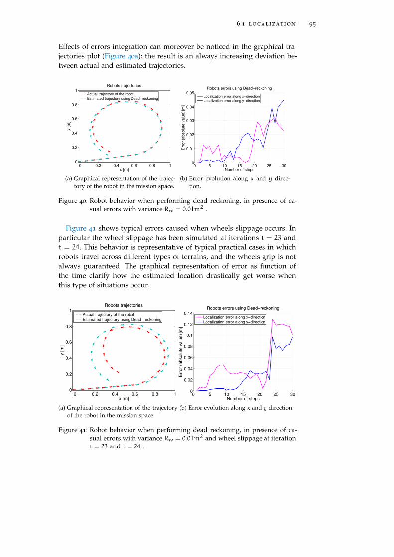
6.1 localization 95
Effects of errors integration can moreover be noticed in the graphical tra-jectories plot (Figure 40a): the result is an always increasing deviation be-tween actual and estimated trajectories.
0 0.2 0.4 0.6 0.8 10
0.2
0.4
0.6
0.8
1
x [m]
y [
m]
Robots trajectories
Actual trajectory of the robot
Estimated trajectory using Dead−reckoning
(a) Graphical representation of the trajec-tory of the robot in the mission space.
0 5 10 15 20 25 300
0.01
0.02
0.03
0.04
0.05
Number of steps
Err
or
(ab
so
lute
va
lue
) [m
]
Robots errors using Dead−reckoning
Localization error along x−direction
Localization error along y−direction
(b) Error evolution along x and y direc-tion.
Figure 40: Robot behavior when performing dead reckoning, in presence of ca-sual errors with variance Rw = 0.01m2 .
Figure 41 shows typical errors caused when wheels slippage occurs. Inparticular the wheel slippage has been simulated at iterations t = 23 andt = 24. This behavior is representative of typical practical cases in whichrobots travel across different types of terrains, and the wheels grip is notalways guaranteed. The graphical representation of error as function ofthe time clarify how the estimated location drastically get worse whenthis type of situations occur.
0 0.2 0.4 0.6 0.8 10
0.2
0.4
0.6
0.8
1
x [m]
y [
m]
Robots trajectories
Actual trajectory of the robot
Estimated trajectory using Dead−reckoning
(a) Graphical representation of the trajectoryof the robot in the mission space.
0 5 10 15 20 25 300
0.02
0.04
0.06
0.08
0.1
0.12
0.14
Number of steps
Err
or
(ab
so
lute
va
lue
) [m
]
Robots errors using Dead−reckoning
Localization error along x−direction
Localization error along y−direction
(b) Error evolution along x and y direction.
Figure 41: Robot behavior when performing dead reckoning, in presence of ca-sual errors with variance Rw = 0.01m2 and wheel slippage at iterationt = 23 and t = 24 .
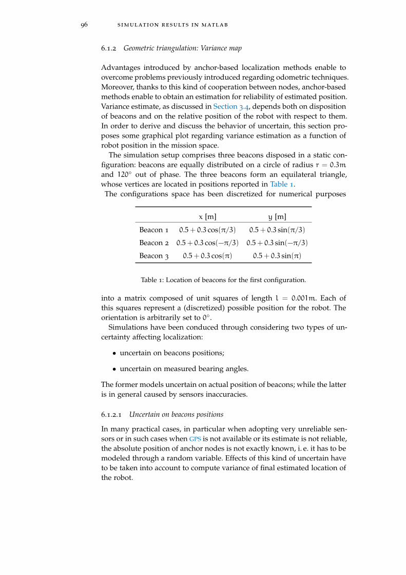
96 simulation results in matlab
6.1.2 Geometric triangulation: Variance map
Advantages introduced by anchor-based localization methods enable toovercome problems previously introduced regarding odometric techniques.Moreover, thanks to this kind of cooperation between nodes, anchor-basedmethods enable to obtain an estimation for reliability of estimated position.Variance estimate, as discussed in Section 3.4, depends both on dispositionof beacons and on the relative position of the robot with respect to them.In order to derive and discuss the behavior of uncertain, this section pro-poses some graphical plot regarding variance estimation as a function ofrobot position in the mission space.
The simulation setup comprises three beacons disposed in a static con-figuration: beacons are equally distributed on a circle of radius r = 0.3mand 120 out of phase. The three beacons form an equilateral triangle,whose vertices are located in positions reported in Table 1.The configurations space has been discretized for numerical purposes
x [m] y [m]
Beacon 1 0.5+ 0.3 cos(π/3) 0.5+ 0.3 sin(π/3)
Beacon 2 0.5+ 0.3 cos(−π/3) 0.5+ 0.3 sin(−π/3)
Beacon 3 0.5+ 0.3 cos(π) 0.5+ 0.3 sin(π)
Table 1: Location of beacons for the first configuration.
into a matrix composed of unit squares of length l = 0.001m. Each ofthis squares represent a (discretized) possible position for the robot. Theorientation is arbitrarily set to 0.
Simulations have been conduced through considering two types of un-certainty affecting localization:
• uncertain on beacons positions;
• uncertain on measured bearing angles.
The former models uncertain on actual position of beacons; while the latteris in general caused by sensors inaccuracies.
6.1.2.1 Uncertain on beacons positions
In many practical cases, in particular when adopting very unreliable sen-sors or in such cases when GPS is not available or its estimate is not reliable,the absolute position of anchor nodes is not exactly known, i. e. it has to bemodeled through a random variable. Effects of this kind of uncertain haveto be taken into account to compute variance of final estimated location ofthe robot.
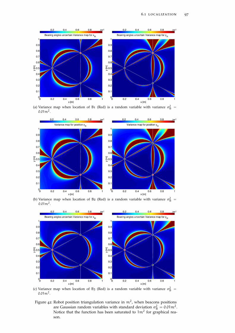
6.1 localization 97
(a) Variance map when location of B1 (Red) is a random variable with variance σ2B =
0.01m2.
(b) Variance map when location of B2 (Red) is a random variable with variance σ2B =
0.01m2.
(c) Variance map when location of B3 (Red) is a random variable with variance σ2B =
0.01m2.
Figure 42: Robot position triangulation variance in m2, when beacons positionsare Gaussian random variables with standard deviation σ2B = 0.01m2.Notice that the function has been saturated to 1m2 for graphical rea-son.
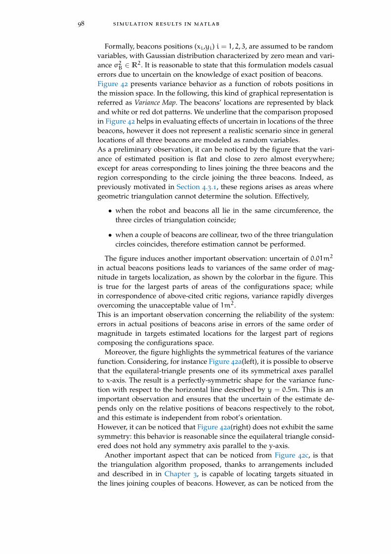
98 simulation results in matlab
Formally, beacons positions (xi,yi) i = 1, 2, 3, are assumed to be randomvariables, with Gaussian distribution characterized by zero mean and vari-ance σ2B ∈ R2. It is reasonable to state that this formulation models casualerrors due to uncertain on the knowledge of exact position of beacons.Figure 42 presents variance behavior as a function of robots positions inthe mission space. In the following, this kind of graphical representation isreferred as Variance Map. The beacons’ locations are represented by blackand white or red dot patterns. We underline that the comparison proposedin Figure 42 helps in evaluating effects of uncertain in locations of the threebeacons, however it does not represent a realistic scenario since in generallocations of all three beacons are modeled as random variables.As a preliminary observation, it can be noticed by the figure that the vari-ance of estimated position is flat and close to zero almost everywhere;except for areas corresponding to lines joining the three beacons and theregion corresponding to the circle joining the three beacons. Indeed, aspreviously motivated in Section 4.3.1, these regions arises as areas wheregeometric triangulation cannot determine the solution. Effectively,
• when the robot and beacons all lie in the same circumference, thethree circles of triangulation coincide;
• when a couple of beacons are collinear, two of the three triangulationcircles coincides, therefore estimation cannot be performed.
The figure induces another important observation: uncertain of 0.01m2
in actual beacons positions leads to variances of the same order of mag-nitude in targets localization, as shown by the colorbar in the figure. Thisis true for the largest parts of areas of the configurations space; whilein correspondence of above-cited critic regions, variance rapidly divergesovercoming the unacceptable value of 1m2.This is an important observation concerning the reliability of the system:errors in actual positions of beacons arise in errors of the same order ofmagnitude in targets estimated locations for the largest part of regionscomposing the configurations space.
Moreover, the figure highlights the symmetrical features of the variancefunction. Considering, for instance Figure 42a(left), it is possible to observethat the equilateral-triangle presents one of its symmetrical axes parallelto x-axis. The result is a perfectly-symmetric shape for the variance func-tion with respect to the horizontal line described by y = 0.5m. This is animportant observation and ensures that the uncertain of the estimate de-pends only on the relative positions of beacons respectively to the robot,and this estimate is independent from robot’s orientation.However, it can be noticed that Figure 42a(right) does not exhibit the samesymmetry: this behavior is reasonable since the equilateral triangle consid-ered does not hold any symmetry axis parallel to the y-axis.
Another important aspect that can be noticed from Figure 42c, is thatthe triangulation algorithm proposed, thanks to arrangements includedand described in in Chapter 3, is capable of locating targets situated inthe lines joining couples of beacons. However, as can be noticed from the
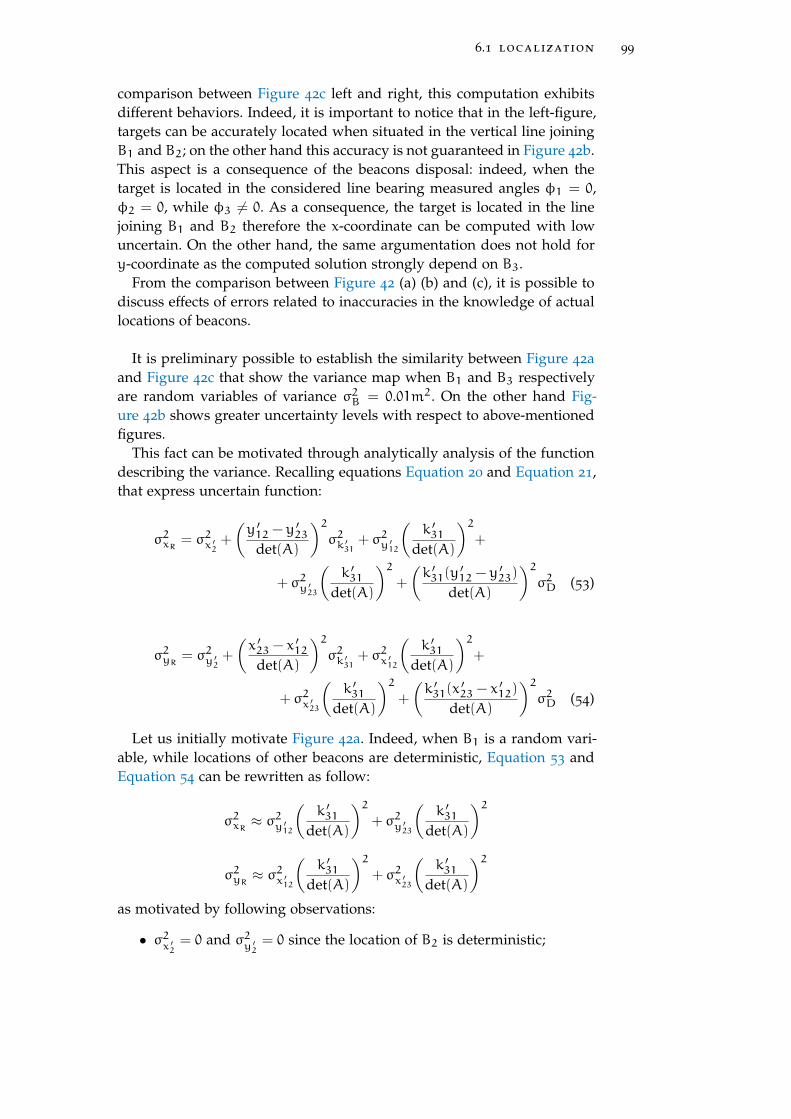
6.1 localization 99
comparison between Figure 42c left and right, this computation exhibitsdifferent behaviors. Indeed, it is important to notice that in the left-figure,targets can be accurately located when situated in the vertical line joiningB1 and B2; on the other hand this accuracy is not guaranteed in Figure 42b.This aspect is a consequence of the beacons disposal: indeed, when thetarget is located in the considered line bearing measured angles φ1 = 0,φ2 = 0, while φ3 6= 0. As a consequence, the target is located in the linejoining B1 and B2 therefore the x-coordinate can be computed with lowuncertain. On the other hand, the same argumentation does not hold fory-coordinate as the computed solution strongly depend on B3.
From the comparison between Figure 42 (a) (b) and (c), it is possible todiscuss effects of errors related to inaccuracies in the knowledge of actuallocations of beacons.
It is preliminary possible to establish the similarity between Figure 42aand Figure 42c that show the variance map when B1 and B3 respectivelyare random variables of variance σ2B = 0.01m2. On the other hand Fig-ure 42b shows greater uncertainty levels with respect to above-mentionedfigures.
This fact can be motivated through analytically analysis of the functiondescribing the variance. Recalling equations Equation 20 and Equation 21,that express uncertain function:
σ2xR = σ2x ′2+
(y ′12 − y
′23
det(A)
)2σ2k ′31
+ σ2y ′12
(k ′31
det(A)
)2+
+ σ2y ′23
(k ′31
det(A)
)2+
(k ′31(y
′12 − y
′23)
det(A)
)2σ2D (53)
σ2yR = σ2y ′2+
(x ′23 − x
′12
det(A)
)2σ2k ′31
+ σ2x ′12
(k ′31
det(A)
)2+
+ σ2x ′23
(k ′31
det(A)
)2+
(k ′31(x
′23 − x
′12)
det(A)
)2σ2D (54)
Let us initially motivate Figure 42a. Indeed, when B1 is a random vari-able, while locations of other beacons are deterministic, Equation 53 andEquation 54 can be rewritten as follow:
σ2xR ≈ σ2y ′12
(k ′31
det(A)
)2+ σ2y ′23
(k ′31
det(A)
)2
σ2yR ≈ σ2x ′12
(k ′31
det(A)
)2+ σ2x ′23
(k ′31
det(A)
)2as motivated by following observations:
• σ2x ′2
= 0 and σ2y ′2
= 0 since the location of B2 is deterministic;

100 simulation results in matlab
•(y ′12−y
′23
det(A)
)2σ2k ′31
= 0 and(x ′23−x
′12
det(A)
)2σ2k ′31
= 0 since σ2k ′31
depends
only on bearing angles variances, and these are assumed determinis-tic;
•(k ′31(y
′12−y
′23)
det(A)
)2σ2D and
(k ′31(x
′23−x
′12)
det(A)
)2σ2D can be neglected.
Equations highlight the strict dependence of estimate position from vari-ances of two of the three triangulation circles centers: (σ2
x ′12; σ2y ′12
) and
(σ2x ′23
; σ2y ′23
). Figure 43 explains circles involved in the solution of the trian-gulation problem.
Figure 43: Circle centers of only two triangulation circles are involved in Equa-tion 53 and Equation 54.
As can be noticed by the figure, uncertain on the knowledge on positionof B1 lead to uncertain in the circle C12 center only, since C13 is not in-volved in Equation 53 and Equation 54. Analogous considerations can beconduced for Figure 42c.
On the other hand, when we consider Figure 42b, it is easy to noticethat uncertainty in the knowledge of location of the node B2 leads un-certain in the knowledge of both C12 and C23 circles centers coordinated.Moreover in this case, additional terms σ2
x ′12and σ2
y ′12in Equation 53 and
Equation 54 cannot be neglected. This observation motivates the greateruncertain levels in Figure 42b.
Finally it is important to underline the key role played by beacon B2that differs from other beacons. This is a consequence of the choice oftranslating the reference frame in the coordinates of B2. Therefore, a goodproject choice is to locate fundamental reference frame on the more precisebeacon. That is, B2 has to be chosen the more precise node.
6.1.2.2 Uncertain on bearing angles
In practical applications for localization we have to deal with non-idealmeasured bearing angles between the robot and beacons. This behaviorcan be caused, for instance, by finite resolution of bearing sensors mounted
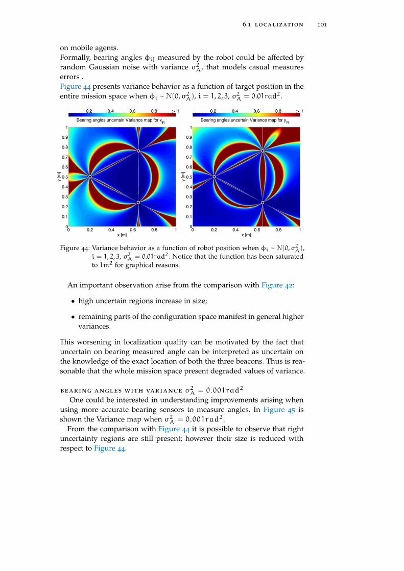
6.1 localization 101
on mobile agents.Formally, bearing angles φij measured by the robot could be affected byrandom Gaussian noise with variance σ2A, that models casual measureserrors .Figure 44 presents variance behavior as a function of target position in theentire mission space when φi ∼ N(0,σ2A), i = 1, 2, 3, σ
2A = 0.01rad2.
Figure 44: Variance behavior as a function of robot position when φi ∼ N(0,σ2A),i = 1, 2, 3, σ2A = 0.01rad2. Notice that the function has been saturatedto 1m2 for graphical reasons.
An important observation arise from the comparison with Figure 42:
• high uncertain regions increase in size;
• remaining parts of the configuration space manifest in general highervariances.
This worsening in localization quality can be motivated by the fact thatuncertain on bearing measured angle can be interpreted as uncertain onthe knowledge of the exact location of both the three beacons. Thus is rea-sonable that the whole mission space present degraded values of variance.
bearing angles with variance σ2A = 0 .001rad2
One could be interested in understanding improvements arising whenusing more accurate bearing sensors to measure angles. In Figure 45 isshown the Variance map when σ2A = 0 .001rad2 .
From the comparison with Figure 44 it is possible to observe that rightuncertainty regions are still present; however their size is reduced withrespect to Figure 44.
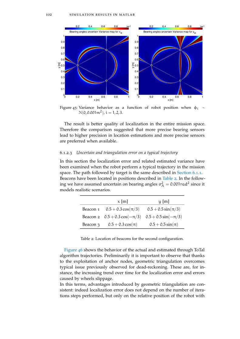
102 simulation results in matlab
Figure 45: Variance behavior as a function of robot position when φi ∼
N(0, 0.001m2), i = 1, 2, 3.
The result is better quality of localization in the entire mission space.Therefore the comparison suggested that more precise bearing sensorslead to higher precision in location estimations and more precise sensorsare preferred when available.
6.1.2.3 Uncertain and triangulation error on a typical trajectory
In this section the localization error and related estimated variance havebeen examined when the robot perform a typical trajectory in the missionspace. The path followed by target is the same described in Section 6.1.1.Beacons have been located in positions described in Table 2. In the follow-ing we have assumed uncertain on bearing angles σ2A = 0.001rad2 since itmodels realistic scenarios.
x [m] y [m]
Beacon 1 0.5+ 0.3 cos(π/3) 0.5+ 0.5 sin(π/3)
Beacon 2 0.5+ 0.3 cos(−π/3) 0.5+ 0.5 sin(−π/3)
Beacon 3 0.5+ 0.3 cos(π) 0.5+ 0.5 sin(π)
Table 2: Location of beacons for the second configuration.
Figure 46 shows the behavior of the actual and estimated through ToTalalgorithm trajectories. Preliminarily it is important to observe that thanksto the exploitation of anchor nodes, geometric triangulation overcomestypical issue previously observed for dead-reckoning. These are, for in-stance, the increasing trend over time for the localization error and errorscaused by wheels slippage.In this terms, advantages introduced by geometric triangulation are con-sistent: indeed localization error does not depend on the number of itera-tions steps performed, but only on the relative position of the robot with
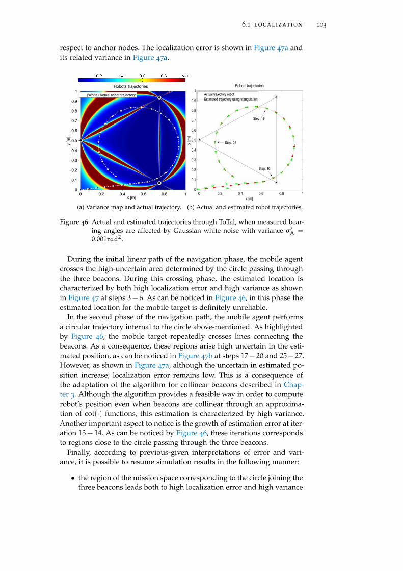
6.1 localization 103
respect to anchor nodes. The localization error is shown in Figure 47a andits related variance in Figure 47a.
(a) Variance map and actual trajectory. (b) Actual and estimated robot trajectories.
Figure 46: Actual and estimated trajectories through ToTal, when measured bear-ing angles are affected by Gaussian white noise with variance σ2A =
0.001rad2.
During the initial linear path of the navigation phase, the mobile agentcrosses the high-uncertain area determined by the circle passing throughthe three beacons. During this crossing phase, the estimated location ischaracterized by both high localization error and high variance as shownin Figure 47 at steps 3− 6. As can be noticed in Figure 46, in this phase theestimated location for the mobile target is definitely unreliable.
In the second phase of the navigation path, the mobile agent performsa circular trajectory internal to the circle above-mentioned. As highlightedby Figure 46, the mobile target repeatedly crosses lines connecting thebeacons. As a consequence, these regions arise high uncertain in the esti-mated position, as can be noticed in Figure 47b at steps 17− 20 and 25− 27.However, as shown in Figure 47a, although the uncertain in estimated po-sition increase, localization error remains low. This is a consequence ofthe adaptation of the algorithm for collinear beacons described in Chap-ter 3. Although the algorithm provides a feasible way in order to computerobot’s position even when beacons are collinear through an approxima-tion of cot(·) functions, this estimation is characterized by high variance.Another important aspect to notice is the growth of estimation error at iter-ation 13− 14. As can be noticed by Figure 46, these iterations correspondsto regions close to the circle passing through the three beacons.
Finally, according to previous-given interpretations of error and vari-ance, it is possible to resume simulation results in the following manner:
• the region of the mission space corresponding to the circle joining thethree beacons leads both to high localization error and high variance
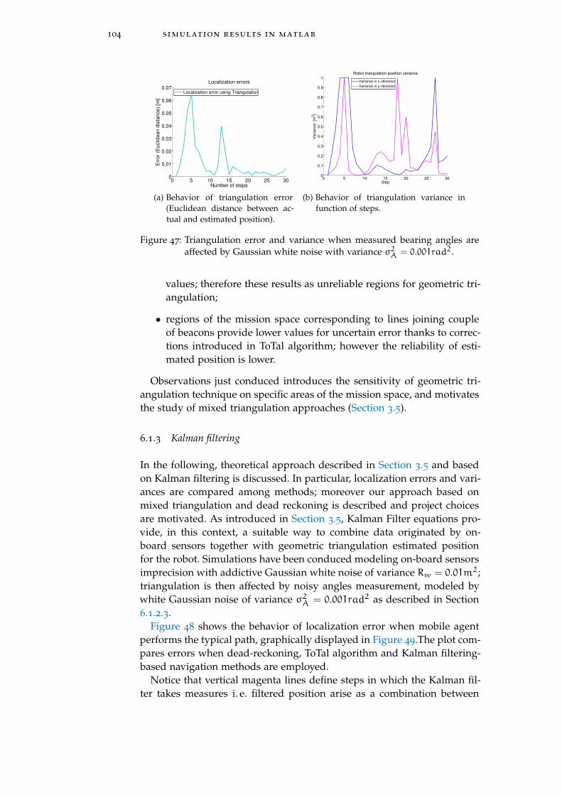
104 simulation results in matlab
0 5 10 15 20 25 300
0.01
0.02
0.03
0.04
0.05
0.06
0.07
Number of steps
Err
or
(Euclid
ean d
ista
nce)
[m]
Localization errors
Localization error using Triangulation
(a) Behavior of triangulation error(Euclidean distance between ac-tual and estimated position).
0 5 10 15 20 25 300
0.1
0.2
0.3
0.4
0.5
0.6
0.7
0.8
0.9
1
Step
Variance [m
2]
Robot triangulation position variance
Variance in x−direction
Variance in y−direction
(b) Behavior of triangulation variance infunction of steps.
Figure 47: Triangulation error and variance when measured bearing angles areaffected by Gaussian white noise with variance σ2A = 0.001rad2.
values; therefore these results as unreliable regions for geometric tri-angulation;
• regions of the mission space corresponding to lines joining coupleof beacons provide lower values for uncertain error thanks to correc-tions introduced in ToTal algorithm; however the reliability of esti-mated position is lower.
Observations just conduced introduces the sensitivity of geometric tri-angulation technique on specific areas of the mission space, and motivatesthe study of mixed triangulation approaches (Section 3.5).
6.1.3 Kalman filtering
In the following, theoretical approach described in Section 3.5 and basedon Kalman filtering is discussed. In particular, localization errors and vari-ances are compared among methods; moreover our approach based onmixed triangulation and dead reckoning is described and project choicesare motivated. As introduced in Section 3.5, Kalman Filter equations pro-vide, in this context, a suitable way to combine data originated by on-board sensors together with geometric triangulation estimated positionfor the robot. Simulations have been conduced modeling on-board sensorsimprecision with addictive Gaussian white noise of variance Rw = 0.01m2;triangulation is then affected by noisy angles measurement, modeled bywhite Gaussian noise of variance σ2A = 0.001rad2 as described in Section6.1.2.3.
Figure 48 shows the behavior of localization error when mobile agentperforms the typical path, graphically displayed in Figure 49.The plot com-pares errors when dead-reckoning, ToTal algorithm and Kalman filtering-based navigation methods are employed.
Notice that vertical magenta lines define steps in which the Kalman fil-ter takes measures i. e. filtered position arise as a combination between

6.1 localization 105
0 5 10 15 20 25 300
0.02
0.04
0.06
0.08
0.1
Number of steps
Err
or
(Eu
clid
ea
n d
ista
nce
) [m
]
Localization errors
Localization error using Dead−Reckoning
Localization error using Triangulation
Localization error using Kalman filtering
Figure 48: Behavior of triangulation error (Euclidean distance from actual posi-tion of the robot). Comparison between Dead-reckoning, ToTal triangu-lation algorithm estimation and Kalman-filtered estimated position. Pa-rameters employed: Rw = 0.01m2, σ2A = 0.001rad2, threshold = 0.02.
dead-reckoning and geometric triangulation. On the other hand, in stepsnot marked with magenta lines, the filter produces estimated location bas-ing on kinematic model only; i. e. follows odometric state-space modelre-initialized last iteration at which measures were available.
It can be noticed by Figure 48 that error behavior for dead-reckoning andtriangulation corresponds to previously-motivated trends (Section 6.1.1and 6.1.2.3 respectively).
As introduced in Section 3.5.5, the Kalman filter dispose for intermittentobservations. This assumption has been done in order to render more ro-bust the algorithm. Indeed it is reasonable to assume that in many practicalcases (because of occlusions, limited-range wireless capabilities, errors incommunications etc. ), mobile agents does not dispose for three availablebeacons at any given time. Furthermore this assumption enable to over-come issues related to high-uncertain areas of the mission space describedin Section 4.3.1. On the other hand, one of the main purposes of this workwas to provide a high-rate localization system, capable of working in theentire mission space and overcoming triangulation unreliable regions. Thecombination between a high-rate location system such as odometry, to-gether with reliable properties of geometric triangulation, lead to a systemcapable of combining both characteristics.
The approach we propose, envisage to:
• exploit dead-reckoning to provide high-rate estimated location;
• when perceived localization error overcome a given threshold, trian-gulation is used in order to improve estimated location.
Simulations have been conduced assuming the given threshold equal tothreshold = 0.02m.It is important to underline that in practical situations, agents in generaldo not dispose of perceived localization error, (on which the considered
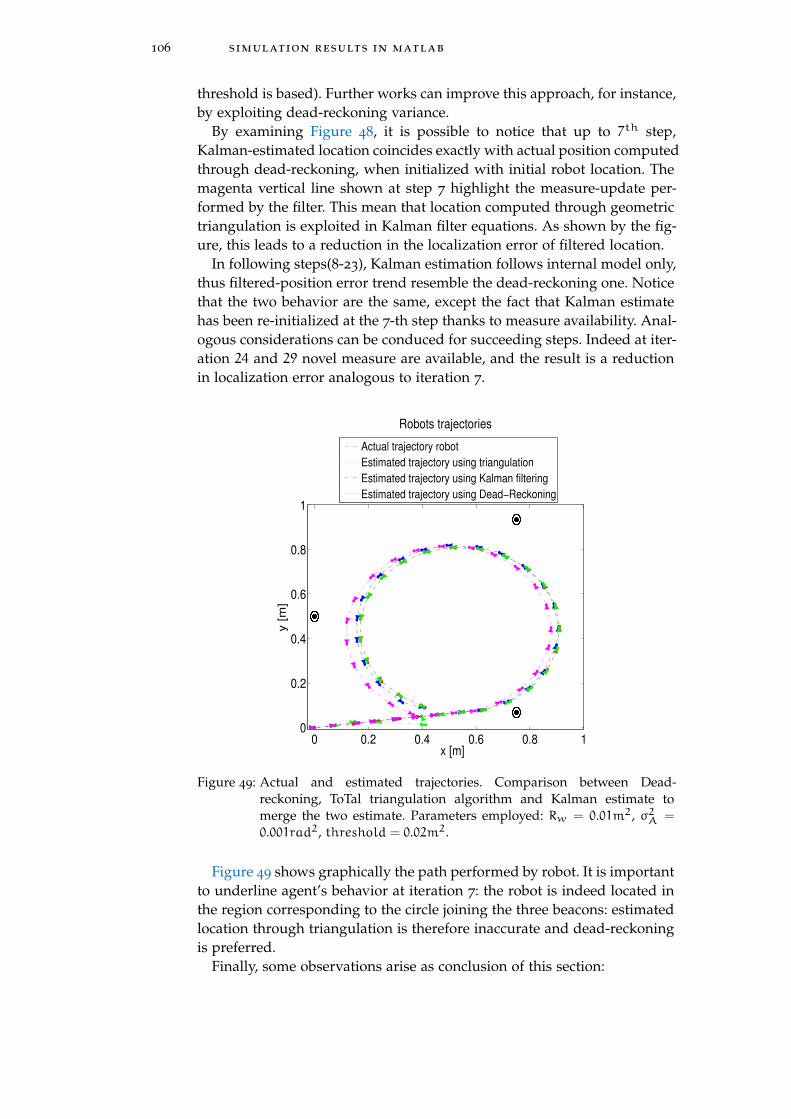
106 simulation results in matlab
threshold is based). Further works can improve this approach, for instance,by exploiting dead-reckoning variance.
By examining Figure 48, it is possible to notice that up to 7th step,Kalman-estimated location coincides exactly with actual position computedthrough dead-reckoning, when initialized with initial robot location. Themagenta vertical line shown at step 7 highlight the measure-update per-formed by the filter. This mean that location computed through geometrictriangulation is exploited in Kalman filter equations. As shown by the fig-ure, this leads to a reduction in the localization error of filtered location.
In following steps(8-23), Kalman estimation follows internal model only,thus filtered-position error trend resemble the dead-reckoning one. Noticethat the two behavior are the same, except the fact that Kalman estimatehas been re-initialized at the 7-th step thanks to measure availability. Anal-ogous considerations can be conduced for succeeding steps. Indeed at iter-ation 24 and 29 novel measure are available, and the result is a reductionin localization error analogous to iteration 7.
0 0.2 0.4 0.6 0.8 10
0.2
0.4
0.6
0.8
1
x [m]
y [m
]
Robots trajectories
Actual trajectory robot
Estimated trajectory using triangulation
Estimated trajectory using Kalman filtering
Estimated trajectory using Dead−Reckoning
Figure 49: Actual and estimated trajectories. Comparison between Dead-reckoning, ToTal triangulation algorithm and Kalman estimate tomerge the two estimate. Parameters employed: Rw = 0.01m2, σ2A =
0.001rad2, threshold = 0.02m2.
Figure 49 shows graphically the path performed by robot. It is importantto underline agent’s behavior at iteration 7: the robot is indeed located inthe region corresponding to the circle joining the three beacons: estimatedlocation through triangulation is therefore inaccurate and dead-reckoningis preferred.
Finally, some observations arise as conclusion of this section:
6.1 localization 107
• geometric triangulation provide accuracy in estimated positions anddoes not suffer of integration-over-time drifts;
• although geometric triangulation provides reliable estimated loca-tions in much regions of the configuration space, there exist someconfined regions where this method is unacceptable;
• dead-reckoning provides simple and high-rate update locations esti-mates, however this method suffers from unbounded error integra-tion that confer unreliability to estimated location;
• the approach we propose is capable of combining advantages of bothmethods, through apposite combination of both model and geomet-ric triangulation.
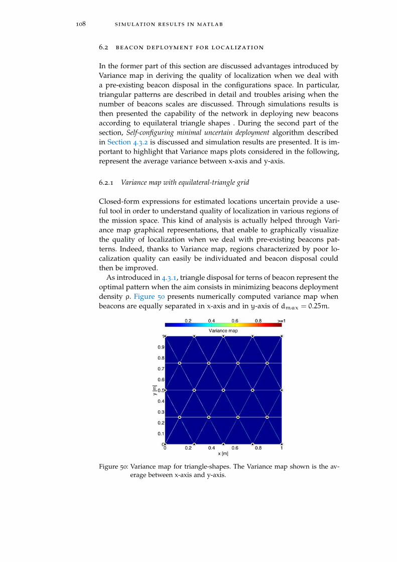
108 simulation results in matlab
6.2 beacon deployment for localization
In the former part of this section are discussed advantages introduced byVariance map in deriving the quality of localization when we deal witha pre-existing beacon disposal in the configurations space. In particular,triangular patterns are described in detail and troubles arising when thenumber of beacons scales are discussed. Through simulations results isthen presented the capability of the network in deploying new beaconsaccording to equilateral triangle shapes . During the second part of thesection, Self-configuring minimal uncertain deployment algorithm describedin Section 4.3.2 is discussed and simulation results are presented. It is im-portant to highlight that Variance maps plots considered in the following,represent the average variance between x-axis and y-axis.
6.2.1 Variance map with equilateral-triangle grid
Closed-form expressions for estimated locations uncertain provide a use-ful tool in order to understand quality of localization in various regions ofthe mission space. This kind of analysis is actually helped through Vari-ance map graphical representations, that enable to graphically visualizethe quality of localization when we deal with pre-existing beacons pat-terns. Indeed, thanks to Variance map, regions characterized by poor lo-calization quality can easily be individuated and beacon disposal couldthen be improved.
As introduced in 4.3.1, triangle disposal for terns of beacon represent theoptimal pattern when the aim consists in minimizing beacons deploymentdensity ρ. Figure 50 presents numerically computed variance map whenbeacons are equally separated in x-axis and in y-axis of dmax = 0.25m.
Figure 50: Variance map for triangle-shapes. The Variance map shown is the av-erage between x-axis and y-axis.
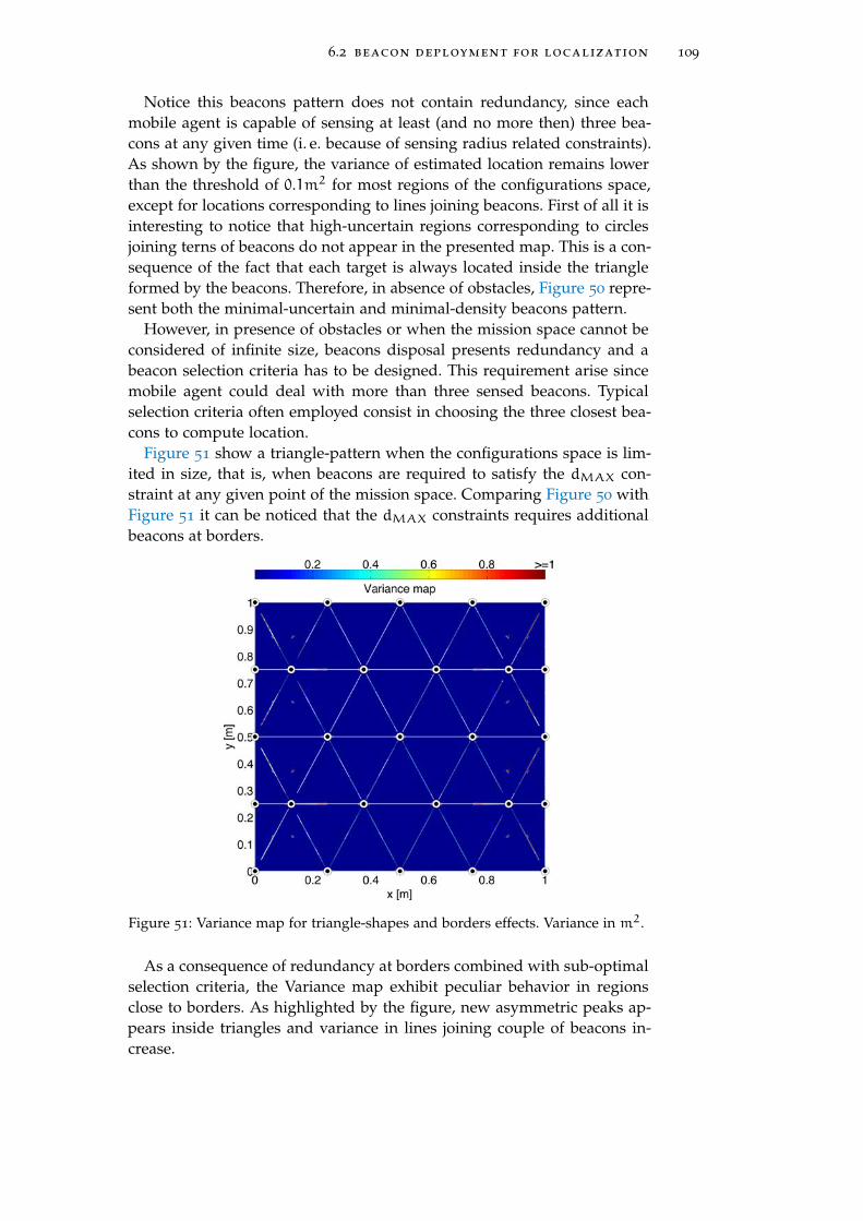
6.2 beacon deployment for localization 109
Notice this beacons pattern does not contain redundancy, since eachmobile agent is capable of sensing at least (and no more then) three bea-cons at any given time (i. e. because of sensing radius related constraints).As shown by the figure, the variance of estimated location remains lowerthan the threshold of 0.1m2 for most regions of the configurations space,except for locations corresponding to lines joining beacons. First of all it isinteresting to notice that high-uncertain regions corresponding to circlesjoining terns of beacons do not appear in the presented map. This is a con-sequence of the fact that each target is always located inside the triangleformed by the beacons. Therefore, in absence of obstacles, Figure 50 repre-sent both the minimal-uncertain and minimal-density beacons pattern.
However, in presence of obstacles or when the mission space cannot beconsidered of infinite size, beacons disposal presents redundancy and abeacon selection criteria has to be designed. This requirement arise sincemobile agent could deal with more than three sensed beacons. Typicalselection criteria often employed consist in choosing the three closest bea-cons to compute location.
Figure 51 show a triangle-pattern when the configurations space is lim-ited in size, that is, when beacons are required to satisfy the dMAX con-straint at any given point of the mission space. Comparing Figure 50 withFigure 51 it can be noticed that the dMAX constraints requires additionalbeacons at borders.
Figure 51: Variance map for triangle-shapes and borders effects. Variance in m2.
As a consequence of redundancy at borders combined with sub-optimalselection criteria, the Variance map exhibit peculiar behavior in regionsclose to borders. As highlighted by the figure, new asymmetric peaks ap-pears inside triangles and variance in lines joining couple of beacons in-crease.
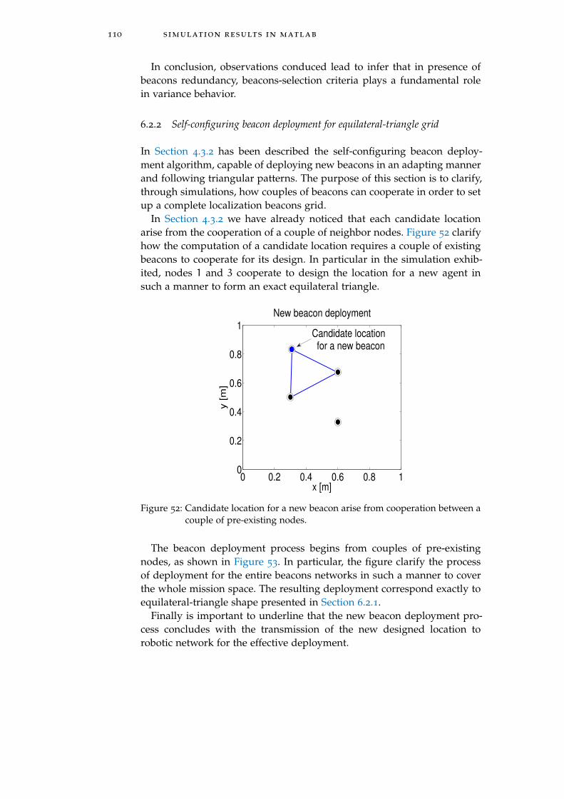
110 simulation results in matlab
In conclusion, observations conduced lead to infer that in presence ofbeacons redundancy, beacons-selection criteria plays a fundamental rolein variance behavior.
6.2.2 Self-configuring beacon deployment for equilateral-triangle grid
In Section 4.3.2 has been described the self-configuring beacon deploy-ment algorithm, capable of deploying new beacons in an adapting mannerand following triangular patterns. The purpose of this section is to clarify,through simulations, how couples of beacons can cooperate in order to setup a complete localization beacons grid.
In Section 4.3.2 we have already noticed that each candidate locationarise from the cooperation of a couple of neighbor nodes. Figure 52 clarifyhow the computation of a candidate location requires a couple of existingbeacons to cooperate for its design. In particular in the simulation exhib-ited, nodes 1 and 3 cooperate to design the location for a new agent insuch a manner to form an exact equilateral triangle.
0 0.2 0.4 0.6 0.8 10
0.2
0.4
0.6
0.8
1Candidate location for a new beacon
x [m]
y [m
]
New beacon deployment
Figure 52: Candidate location for a new beacon arise from cooperation between acouple of pre-existing nodes.
The beacon deployment process begins from couples of pre-existingnodes, as shown in Figure 53. In particular, the figure clarify the processof deployment for the entire beacons networks in such a manner to coverthe whole mission space. The resulting deployment correspond exactly toequilateral-triangle shape presented in Section 6.2.1.
Finally is important to underline that the new beacon deployment pro-cess concludes with the transmission of the new designed location torobotic network for the effective deployment.
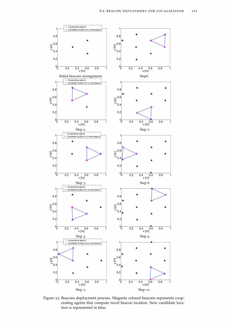
6.2 beacon deployment for localization 111
0 0.2 0.4 0.6 0.8 10
0.2
0.4
0.6
0.8
1
x [m]
y [m
]
Cooperating agents
Candidate location for a new beacon
Initial beacons arrangement.
0 0.2 0.4 0.6 0.8 10
0.2
0.4
0.6
0.8
1
x [m]
y [m
]
Step6.
0 0.2 0.4 0.6 0.8 10
0.2
0.4
0.6
0.8
1
x [m]
y [m
]
Cooperating agents
Candidate location for a new beacon
Step 2.
0 0.2 0.4 0.6 0.8 10
0.2
0.4
0.6
0.8
1
x [m]
y [m
]
Step 7.
0 0.2 0.4 0.6 0.8 10
0.2
0.4
0.6
0.8
1
x [m]
y [
m]
Cooperating agents
Candidate location for a new beacon
Step 3.
0 0.2 0.4 0.6 0.8 10
0.2
0.4
0.6
0.8
1
x [m]
y [m
]
Step 8.
0 0.2 0.4 0.6 0.8 10
0.2
0.4
0.6
0.8
1
x [m]
y [m
]
Cooperating agents
Candidate location for a new beacon
Step 4.
0 0.2 0.4 0.6 0.8 10
0.2
0.4
0.6
0.8
1
x [m]
y [m
]
Step 9.
0 0.2 0.4 0.6 0.8 10
0.2
0.4
0.6
0.8
1
x [m]
y [m
]
Cooperating agents
Candidate location for a new beacon
Step 5.
0 0.2 0.4 0.6 0.8 10
0.2
0.4
0.6
0.8
1
x [m]
y [
m]
Step 10.
Figure 53: Beacons deployment process. Magenta colored beacons represents coop-erating agents that compute novel beacon location. New candidate loca-tion is represented in blue.

112 simulation results in matlab
6.2.3 Self-configuring minimal uncertain deployment
When the final objective consists in both minimizing beacons density ρand minimizing beacons locations uncertain, triangle shapes have to bemodified and the computed candidate location arise as the solution ofan optimization problem. In this section, we propose simulations resultswhen implementing Algorithm 4.Figure 54 proposes a typical situation in which locating new beaconsin correspondence of the vertex of the equilateral triangle gives rise tounacceptable uncertain in new beacon’s location. Indeed, candidate loca-tion corresponding to vertex of equilateral triangle, correspond to a high-uncertain region since it lies on a line joining a couple of beacons.
Figure 54: Minimal uncertain deployment. Ultimate candidate location is repre-sented in green colour.
As highlighted by the figure, the optimization process enable to avoidthis undesired behavior by modifying candidate location.
Figure 55 show the minimal uncertain deployment process when nodesemploy Algorithm 4.In order to lead the network to maintain a certain triangle-like structure,the optimization was performed weighing distances between candidatelocation and actual triplet. That is, following the algorithm:
Algorithm 5 Iterative deployment algorithm weighted on distances
1) Send request to neighbors for their positions;2) Compute acceptable positions Ω respecting the dMAX constraint;3) Compute the variance map;4) Solve the constrained optimization:
minΩ V(x,y) · dist(x,y), (x∗,y∗)−1;5) Compute ultimate candidate position through average consensus
with immediate neighbor.
where (x∗,y∗) represent current beacon position.
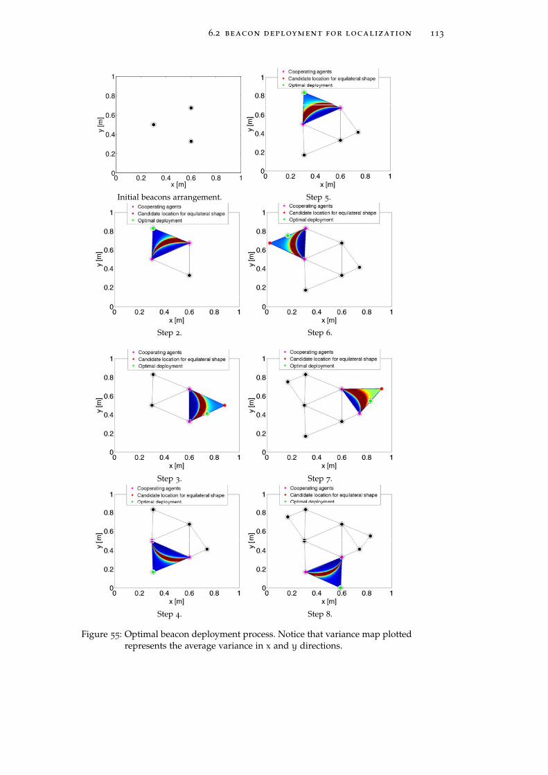
6.2 beacon deployment for localization 113
0 0.2 0.4 0.6 0.8 10
0.2
0.4
0.6
0.8
1
x [m]
y [m
]
Initial beacons arrangement. Step 5.
Step 2. Step 6.
Step 3. Step 7.
Step 4. Step 8.
Figure 55: Optimal beacon deployment process. Notice that variance map plottedrepresents the average variance in x and y directions.
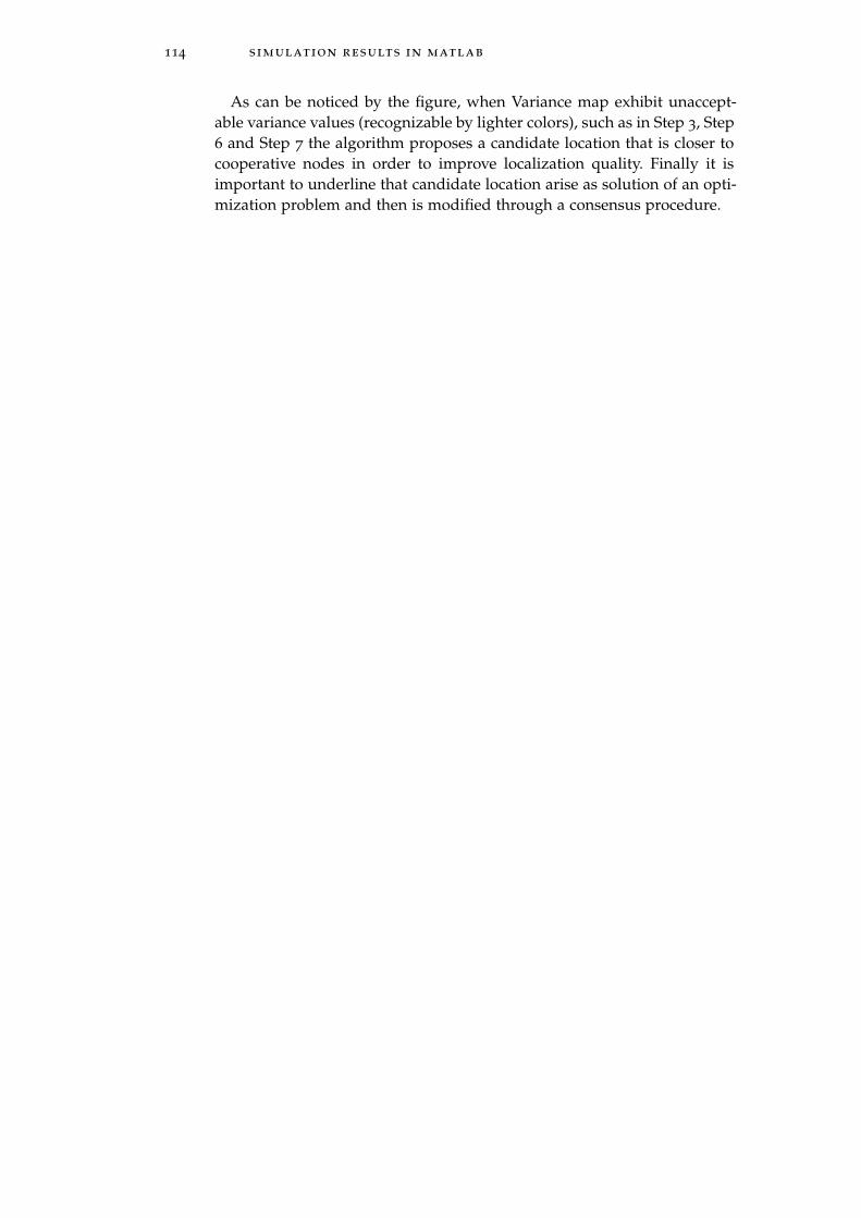
114 simulation results in matlab
As can be noticed by the figure, when Variance map exhibit unaccept-able variance values (recognizable by lighter colors), such as in Step 3, Step6 and Step 7 the algorithm proposes a candidate location that is closer tocooperative nodes in order to improve localization quality. Finally it isimportant to underline that candidate location arise as solution of an opti-mization problem and then is modified through a consensus procedure.
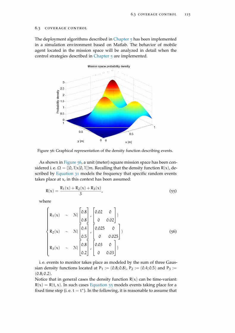
6.3 coverage control 115
6.3 coverage control
The deployment algorithms described in Chapter 5 has been implementedin a simulation environment based on Matlab. The behavior of mobileagent located in the mission space will be analyzed in detail when thecontrol strategies described in Chapter 5 are implemented.
Figure 56: Graphical representation of the density function describing events.
As shown in Figure 56, a unit (meter) square mission space has been con-sidered i. e.Ω = [0, 1]x[0, 1]m. Recalling that the density function R(x), de-scribed by Equation 31 models the frequency that specific random eventstakes place at x, in this context has been assumed:
R(x) =R1(x) + R2(x) + R3(x)
3, (55)
where
R1(x) ∼ N(
0.80.8
,
0.02 0
0 0.02
)R2(x) ∼ N(
0.40.5
,
0.025 0
0 0.025
)R3(x) ∼ N(
0.80.2
,
0.03 0
0 0.03
)(56)
i. e. events to monitor takes place as modeled by the sum of three Gaus-sian density functions located at P1 := (0.8; 0.8), P2 := (0.4; 0.5) and P3 :=
(0.8; 0.2).Notice that in general cases the density function R(x) can be time-variant:R(x) = R(t, x). In such cases Equation 55 models events taking place for afixed time step (i. e. t = t∗). In the following, it is reasonable to assume that
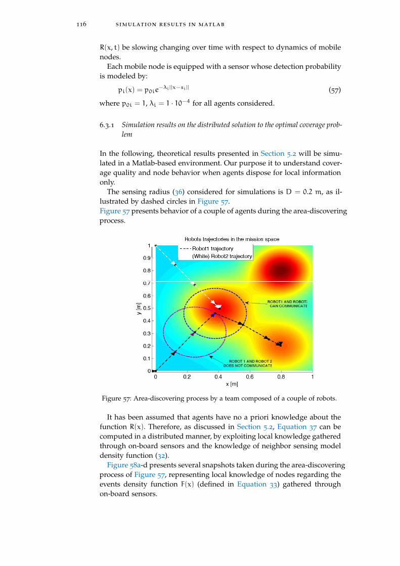
116 simulation results in matlab
R(x, t) be slowing changing over time with respect to dynamics of mobilenodes.
Each mobile node is equipped with a sensor whose detection probabilityis modeled by:
pi(x) = p0ie−λi||x−si|| (57)
where p0i = 1, λi = 1 · 10−4 for all agents considered.
6.3.1 Simulation results on the distributed solution to the optimal coverage prob-lem
In the following, theoretical results presented in Section 5.2 will be simu-lated in a Matlab-based environment. Our purpose it to understand cover-age quality and node behavior when agents dispose for local informationonly.
The sensing radius (36) considered for simulations is D = 0.2 m, as il-lustrated by dashed circles in Figure 57.Figure 57 presents behavior of a couple of agents during the area-discoveringprocess.
Figure 57: Area-discovering process by a team composed of a couple of robots.
It has been assumed that agents have no a priori knowledge about thefunction R(x). Therefore, as discussed in Section 5.2, Equation 37 can becomputed in a distributed manner, by exploiting local knowledge gatheredthrough on-board sensors and the knowledge of neighbor sensing modeldensity function (32).
Figure 58a-d presents several snapshots taken during the area-discoveringprocess of Figure 57, representing local knowledge of nodes regarding theevents density function F(x) (defined in Equation 33) gathered throughon-board sensors.
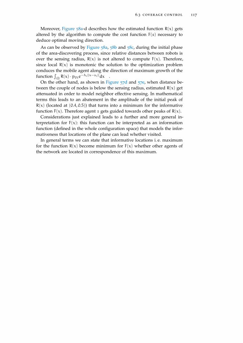
6.3 coverage control 117
Moreover, Figure 58a-d describes how the estimated function R(x) getsaltered by the algorithm to compute the cost function F(s) necessary todeduce optimal moving direction.
As can be observed by Figure 58a, 58b and 58c, during the initial phaseof the area-discovering process, since relative distances between robots isover the sensing radius, R(x) is not altered to compute F(x). Therefore,since local R(x) is monotonic the solution to the optimization problemconduces the mobile agent along the direction of maximum growth of thefunction
∫Ω R(x) · p0ie
−λi||x−si||dx .On the other hand, as shown in Figure 57d and 57e, when distance be-
tween the couple of nodes is below the sensing radius, estimated R(x) getattenuated in order to model neighbor effective sensing. In mathematicalterms this leads to an abatement in the amplitude of the initial peak ofR(x) (located at (0.4, 0.5)) that turns into a minimum for the informativefunction F(x). Therefore agent 1 gets guided towards other peaks of R(x).
Considerations just explained leads to a further and more general in-terpretation for F(x): this function can be interpreted as an informationfunction (defined in the whole configuration space) that models the infor-mativeness that locations of the plane can lead whether visited.
In general terms we can state that informative locations i. e. maximumfor the function R(x) become minimum for F(x) whether other agents ofthe network are located in correspondence of this maximum.
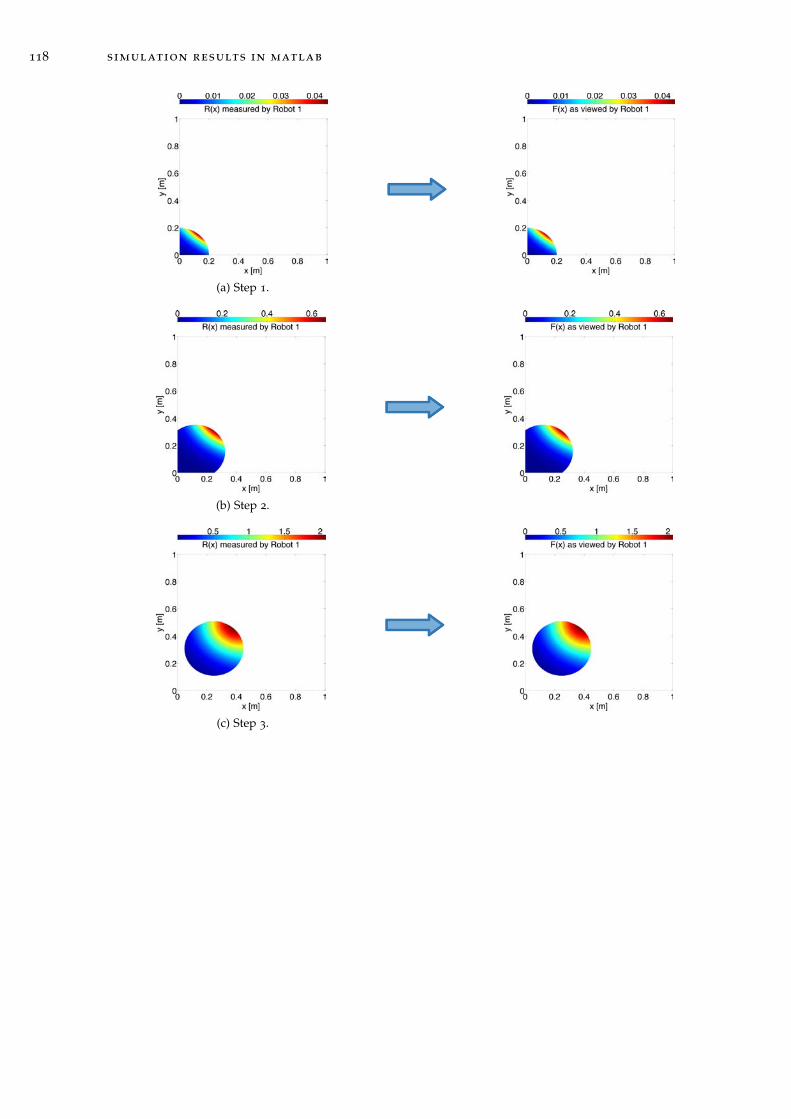
118 simulation results in matlab
(a) Step 1.
(b) Step 2.
(c) Step 3.
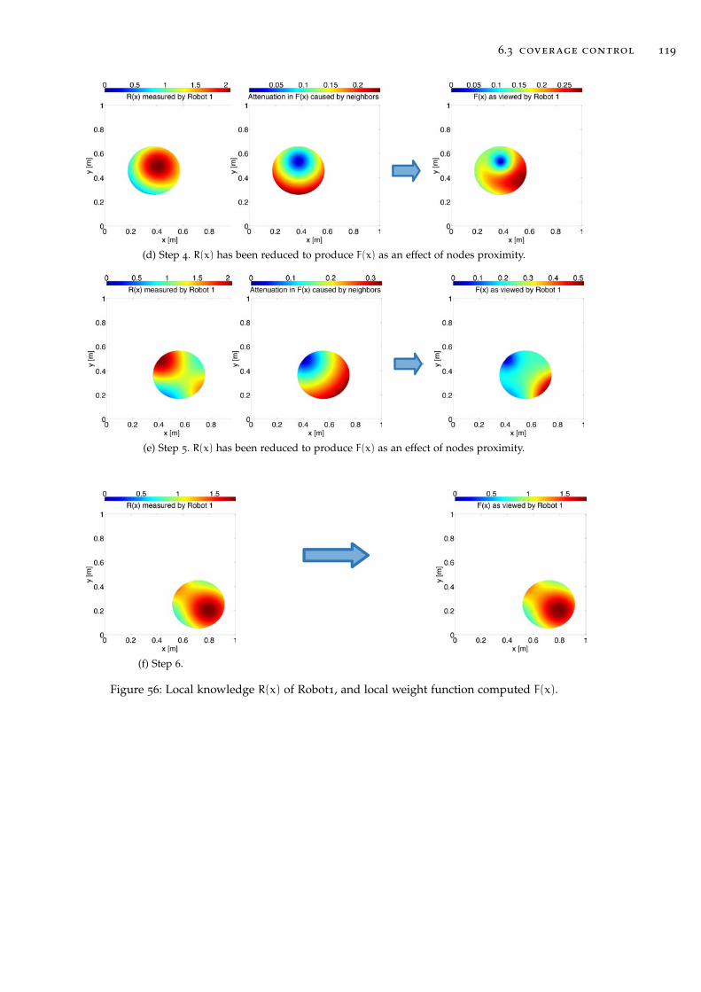
6.3 coverage control 119
(d) Step 4. R(x) has been reduced to produce F(x) as an effect of nodes proximity.
(e) Step 5. R(x) has been reduced to produce F(x) as an effect of nodes proximity.
(f) Step 6.
Figure 56: Local knowledge R(x) of Robot1, and local weight function computed F(x).
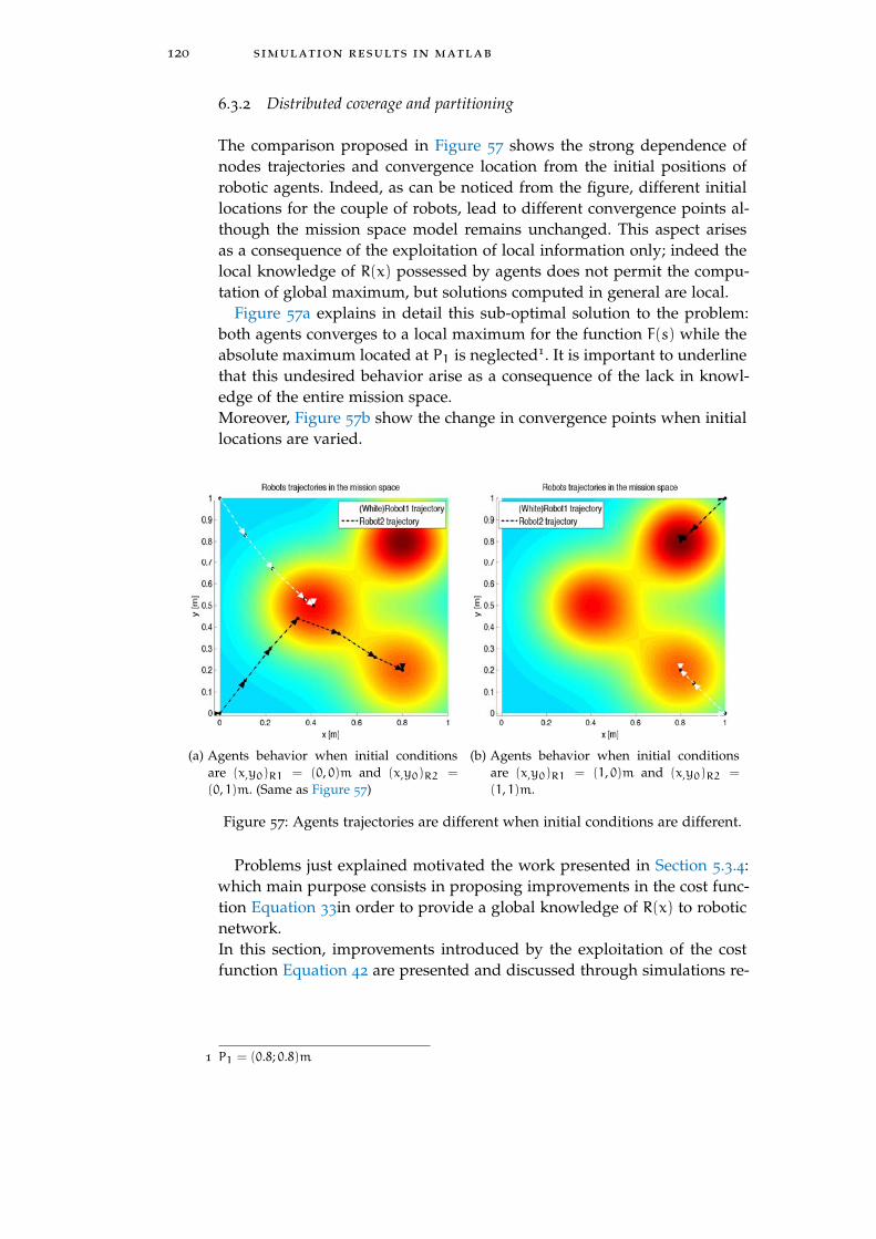
120 simulation results in matlab
6.3.2 Distributed coverage and partitioning
The comparison proposed in Figure 57 shows the strong dependence ofnodes trajectories and convergence location from the initial positions ofrobotic agents. Indeed, as can be noticed from the figure, different initiallocations for the couple of robots, lead to different convergence points al-though the mission space model remains unchanged. This aspect arisesas a consequence of the exploitation of local information only; indeed thelocal knowledge of R(x) possessed by agents does not permit the compu-tation of global maximum, but solutions computed in general are local.
Figure 57a explains in detail this sub-optimal solution to the problem:both agents converges to a local maximum for the function F(s) while theabsolute maximum located at P1 is neglected1. It is important to underlinethat this undesired behavior arise as a consequence of the lack in knowl-edge of the entire mission space.Moreover, Figure 57b show the change in convergence points when initiallocations are varied.
(a) Agents behavior when initial conditionsare (x,y0)R1 = (0, 0)m and (x,y0)R2 =
(0, 1)m. (Same as Figure 57)
(b) Agents behavior when initial conditionsare (x,y0)R1 = (1, 0)m and (x,y0)R2 =
(1, 1)m.
Figure 57: Agents trajectories are different when initial conditions are different.
Problems just explained motivated the work presented in Section 5.3.4:which main purpose consists in proposing improvements in the cost func-tion Equation 33in order to provide a global knowledge of R(x) to roboticnetwork.In this section, improvements introduced by the exploitation of the costfunction Equation 42 are presented and discussed through simulations re-
1 P1 = (0.8; 0.8)m
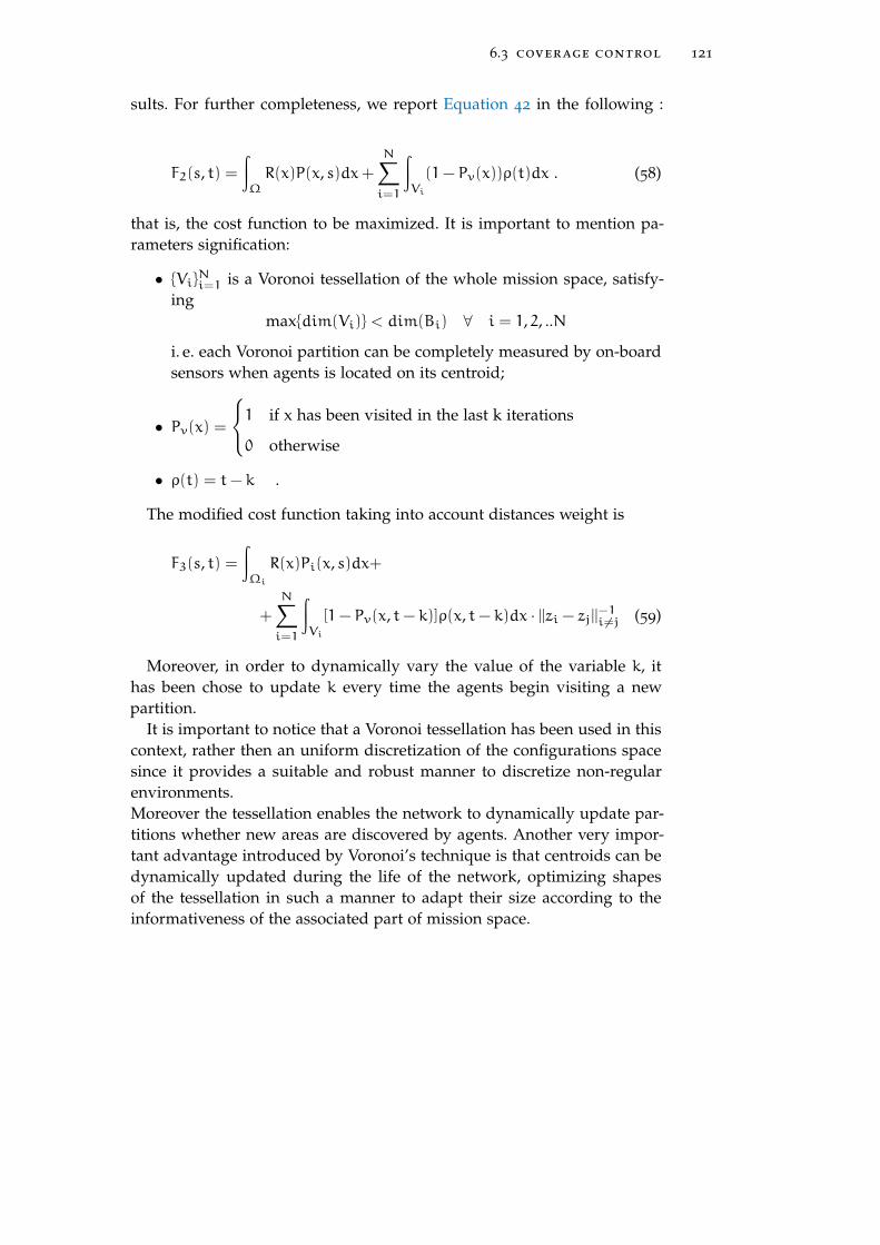
6.3 coverage control 121
sults. For further completeness, we report Equation 42 in the following :
F2(s, t) =∫Ω
R(x)P(x, s)dx+N∑i=1
∫Vi
(1− Pv(x))ρ(t)dx . (58)
that is, the cost function to be maximized. It is important to mention pa-rameters signification:
• ViNi=1 is a Voronoi tessellation of the whole mission space, satisfy-
ingmaxdim(Vi) < dim(Bi) ∀ i = 1, 2, ..N
i. e. each Voronoi partition can be completely measured by on-boardsensors when agents is located on its centroid;
• Pv(x) =
1 if x has been visited in the last k iterations
0 otherwise
• ρ(t) = t− k .
The modified cost function taking into account distances weight is
F3(s, t) =∫Ωi
R(x)Pi(x, s)dx+
+
N∑i=1
∫Vi
[1− Pv(x, t− k)]ρ(x, t− k)dx · ||zi − zj||−1i 6=j (59)
Moreover, in order to dynamically vary the value of the variable k, ithas been chose to update k every time the agents begin visiting a newpartition.
It is important to notice that a Voronoi tessellation has been used in thiscontext, rather then an uniform discretization of the configurations spacesince it provides a suitable and robust manner to discretize non-regularenvironments.Moreover the tessellation enables the network to dynamically update par-titions whether new areas are discovered by agents. Another very impor-tant advantage introduced by Voronoi’s technique is that centroids can bedynamically updated during the life of the network, optimizing shapesof the tessellation in such a manner to adapt their size according to theinformativeness of the associated part of mission space.

122 simulation results in matlab
(a)
0 0.2 0.4 0.6 0.8 10
0.2
0.4
0.6
0.8
1
x [m]
y [
m]
Path graph (Frequency of visits)
Low
High
(b)
Figure 58: (a) Single robot implementing Equation 58 and performing 1000 itera-tions. Notice that every Voronoi location have been visited almost onceand that more rapidly changing locations have been visited more oftenthan other areas. (b) Related graph.
In Figure 58 is shown the behavior of a single robot when implementingEquation 59. Notice that Equation 59 takes into account distances betweencentroids. The plot representing robot’s paths in the mission space is en-hanced by a graph representing frequency at which Voronoi cells are beingvisited; nodes represent Voronoi centroids while edges models sequencesin visits. The mission space model is the same in (56).Figure 58a clarifies the fact that the algorithm leads the robot to visit thewhole mission space, through imposing the visit of every Voronoi cell. Thisleads the robot to build-up a comprehensive knowledge of the configura-tion space and in particular of its model R(x).
6.3 coverage control 123
The graph in Figure 58a graphically show the behavior just explained.Indeed, nodes and edges corresponding to regions with peaks in R(x) re-sults more frequently visited than remaining centroids of the configura-tions space. As a consequence, disposing of a complete knowledge about
(a) (b)
(c) (d)
(e)
Figure 59: Visited partition when exploiting Equation 59.
the mission space, mobile agents are capable of detecting and reachingglobal maximum for R(x). Another important aspect to notice is that highinformative locations are visited more often than border regions. This be-havior is motivated observing that once the robot moves to visit a newpartition, then it moves climbing informativeness gradient so reaching

124 simulation results in matlab
the closest maximum. Therefore we can state that high-informativenessregions are being monitored with higher frequencies.
Figure 59 show visited partitions over time by the robot when perform-ing paths shown in Figure 58. It can be noticed by the figure that thecontrol strategy in about 100 iterations leads the robot to visit almost allgiven partitions.
In order to validate effects introduced by weighting the cost functionwith distances that agents are required to travel in order to reach nextVoronoi cell, the purpose is then to compare (58) and Equation 59.
0 0.2 0.4 0.6 0.8 10
0.2
0.4
0.6
0.8
1
x [m]
y [
m]
Path graph (Frequency of visits)
Low
High
(a) Considering distances costs.
0 0.2 0.4 0.6 0.8 10
0.2
0.4
0.6
0.8
1
x [m]
y [m
]
Path graph (Frequency of visits)
Low
High
(b) Neglecting distances costs.
Figure 60: Graph comparison.
The comparison proposed by Figure 60 highlights advantages in ex-ploiting distances costs in weight function. First of all, it can be noticedthat graph exploiting (58) is highly connected: this is a consequence ofthe higher distances traveled by agents to reach far away locations in themission space. Furthermore the comparison between colors of nodes high-lights how Equation 59 enable the agent to visit more frequently highinformativeness regions.
In Figure 61 evolution of visited partitions over time is compared whenusing Equation 59 and (58). From the comparison it is possible to noticethat when exploiting (58), the robot is requested to travel longer distancesin order to initially visit more interesting partitions. However, althoughmore interesting partitions get visited earlier, the visiting procedure re-quires longer times to converge, since there exist a wasting in time totravel these distances.

6.3 coverage control 125
(a) Covered regions at iteration 50 whenusing (59).
(b) Covered regions at iteration 50 whenusing (58).
(c) Covered regions at iteration 100 whenusing (59).
(d) Covered regions at iteration 100 when us-ing (58).
Figure 61: Comparison between (58) and (59) .

Part IV
C O N C L U S I O N S A N D A P P E N D I X
The following chapters summarize the conclusions of the the-sis an future works. Appendixes containing connected open-problems conclude the part.


7C O N C L U S I O N S
Sensor networks are considered a key technology for the future. Their usehas enlarged rapidly in last decade in view of a future that is increas-ingly automated. Scientific efforts are above all focusing on the develop-ment of smart agent networks, i. e. networks composed by devices able toautonomously sense environment and adapt network features upon mea-sured quantities.
Multi-Robot systems are considered as a promising technology in envi-ronmental monitoring, since they permit to enhance capabilities of sensornetworks by introducing mobility features to sensors employed. However,to achieve this automation, mobile robots must include a localization sys-tem. The growing possibilities enabled by robotic networks in the monitor-ing of natural phenomena, combined with flexibility features typical fordistribute sensor networks, enable a number of potential improvements inquality of service provided in distributed area exploration. This work hasaimed at exploring the fields of work of both sensor and robot networksthrough combining complementary features of these two systems.
This thesis addresses first the problem of locating mobile agents in un-known environments. In this kinds of frameworks, odometric techniquesare the mainly used because of their low cost, high-update rate and accu-racy in short paths. Unlikely, this methods resulted unacceptable in longpaths because of an unbounded growth of time integration error with thetraveled distance. Solutions based on anchor nodes, such as GeometricTriangulation, provides a promising way in order to improve localizationquality in longer paths. However, since no a priori knowledge regardingthe environment is possessed by the network and anchors cannot be lo-cated offline, agents are required to be equipped with mechanisms capableof deploying beacons that can serve for localization. In this terms, we havedesigned a localization system capable of self-deploying the static infras-tructure composed by beacons. Characteristics of Geometric triangulationhave been described in detail, and the method has been taken into accountsince it provides a promising method in anchor-based localization. Ourcontribution leads to derive a closed-form expression for the variance ofestimated target location.Considering the variance of target estimated location as a function of rela-tive position of the target with respect to beacons, the mission space couldbe divided into disjoint regions where the variance is almost zero andregions where the variance presents a divergent behavior. In order to pro-vide a robust, high precision, and high-updating rate system, we proposedan hybrid localization system based on Kalman filter in order to combineodometric readings together with estimated location through geometric
129

130 conclusions
triangulation. Through simulation results we have probed the robustnessof the method, even in typical noisy trajectories.
Deploying capabilities held by mobile agents give rise to the problem ofunderstanding the optimal locations for new beacons in order to extendexisting infrastructure together with improving the quality of the serviceprovided. This problem has resulted to be NP-Hard. The distributed self-deployment algorithm proposed, is based on local cooperation betweenonly two beacons nodes to design new candidate locations. The main fea-ture of the system is the robustness guaranteed by the capability in com-puting actual location of the novel deployed beacon. This lead the systemto work both in indoor and outdoor environments, since no global posi-tioning systems are required.
The performance of sensor and robot systems in terms of quality of theservice provided is sensitive to locations of agents in the mission space.In particular sensors are required to spread over the covered area andto aggregate in high-informativeness regions. This requirement, in contextwhere the mission space model is changing over time, involve a dynamicaldeployment for senors. This feature can be met through the exploitationof mobile vehicles in areas rapidly changing over time, while fixed sensorscan be employed in static areas. This kind of coverage control problems areusually solved through the exploitation of a parametric function modelingfrequencies of events taking place in the configurations space. A novel dis-tributed approach based on local optimization of cost function is proposedfor coverage the control problem. Simulations motivate the introductionof a novel weigh function, capable of providing a global knowledge of theconfigurations space through an initialization process. Simulations resultsand a mathematical rigorous approach demonstrated the capability of thecost function in accurately modeling unknown areas of the mission spacead in leading agents to visit the entire mission space without requiringaccurate path planning.
8F U T U R E W O R K
The application suggests a number of interesting directions for furtherwork. First of all, it would be interesting to analyze the performances ofGeometric Triangulation in presence of obstacles, occlusions, or in pres-ence of further sources of noise in measured bearing angles. In this sense,the derivation of a Variance map can be extended in presence of obstaclesand occlusions. In order to overcome this kind of problems, we suggest toderive a closed form expression for uncertain of estimated position as afunction of the power or the integrity of measured signals.
In Section 6.1.3 the Kalman filter with intermittent observations wasimplemented in order to improve localization quality. However, we havesupposed to exploit observation whenever the perceived localization errorovercomes a fixed threshold. It would be interesting to analyze in detailthis problem; in particular to derive a mathematical model for the per-ceived localization error and propose alternative conditions.One relevant assumption done in Chapter 3 was the absence of noise in es-timated robot orientation. Motivated by many practical approaches whererobot’s orientation is corrupted by noise, future works would require toovercome this assumption. Another relevant issue to threat in localizationwould be the the extension of proposed algorithm in order to exploit re-dundancy in available beacons. The direction for future works we proposeis based on an iterative application of Geometric Triangulation algorithmthat exploits all combination without repetitions of terns of available bea-cons.
In the beacon deployment process, future works could involve an anal-ysis of the quality of service provided as a function of beacons density ρ.Moreover, alternative beacons patterns could be considered, in comparisonwith the equilateral-triangle one proposed in this work.
The distributed coverage control problem was analyzed through the ex-ploitation of a Voronoi tessellation in order to provide a global knowledgeabout the environment to the network. It would be interesting to analyzethe problem through a dynamical tessellation of the mission space. In par-ticular centroids can be located, and regions can be adapted in size soas to consider R(x, t) as a key factor in the tessellation process. Moreover,further works motivated by practical applications could involve missionspaces model R(x) rapidly changing over time: typical applications are,for instance, the tracking of mobile targets.
131

AA P P E N D I X
a.1 communications costs
Besides sensing and collecting data from the mission space Ω, another im-portant issue of a sensor network is to forward fields data to a basestationb, in order to provide real-time responsiveness of the network for externalusers. Most current sensor networks assume a two-layer structure [30], inwhich all sensor nodes form the first layer, and the second layer consistsof a unique basestation, which is the common destination for all data.
In order to ensure reliable data forwarding, a wireless link must pre-serve a certain channel quality, which is measured by its Signal to NoiseRatio (SNR). To preserve a given SNR, the power of the transmitter have tobe taken into account, that is a monotonically increasing function of thelength of the current link. For example, for a single hop wireless link, theenergy needed to transmit (Etx) and receive (Erx) a bit follows:
Etx = γ+βdn
Erx = η
where a 1dn path loss has been assumed and γ is the energy/bit consumed
by the transmitter electronics, β accounts for energy dissipated in the trans-mit op-amp and η is the energy/bit consumed by a node to receive the bit.In this terms, a relay that receives a bit and then transmits it a distance dis:
e(d) = γ+βdn + η = (γ+ η) +βdn +α+βdn .
Typical parameters for current radio transmission are γ = 180nJ/bit, β =
10pJ/bit/m2 n = 2.Considering a mobile sensor network with N sensors, each located at si,
i = 1, . . . ,N, and a single basestation b located at s0 ∈ R2. Let ri(si) bethe data rate originated by the i-th sensor. Note that ri is a function of sibecause the amount of data forwarded at i is determined by the numberof events detected, that is on the sensor location. It is reasonable to assumethat ri(si) is proportional to the frequency at which events are detected,i. e. :
ri(si) = k
∫Ω
R(x)pi(x)dx
where k [bit/detection] is the average amount of data forwarded when thesensor detects an event. Data originated at each sensor have to be finallydelivered to the basestation. Let ci(s) be the total power consumed by thenetwork in order to deliver a bit of data from sensor i to the basestation b.
133
134 appendix
In this terms, the optimal coverage problem can be revised by combiningsensing coverage and communication costs:
maxs
ω1
∫Ω
R(x)P(x, s)dx−ω2N∑i=1
ri(si)ci(s)
where ω1, ω2 are weighting factors. Denoting the communication cost by
G(s) =
N∑i=1
ri(si)ci(s),
the overall objective function can be rewritten as:
J(s) = ω1F(s) −ω2G(s) .

B I B L I O G R A P H Y
[1] James C Alexander and John H Maddocks. On the kinematics ofwheeled mobile robots. In Autonomous robot vehicles, pages 5–24.Springer, 1990.
[2] Johann Borenstein and Yoram Koren. A mobile platform for nursingrobots. Industrial Electronics, IEEE Transactions on, (2):158–165, 1985.
[3] Nirupama Bulusu, John Heidemann, and Deborah Estrin. Adaptivebeacon placement. In Distributed Computing Systems, 2001. 21st Inter-national Conference on., pages 489–498. IEEE, 2001.
[4] Nirupama Bulusu, John Heidemann, Deborah Estrin, and TommyTran. Self-configuring localization systems: Design and experimentalevaluation. ACM Transactions on Embedded Computing Systems (TECS),3(1):24–60, 2004.
[5] Mihaela Cardei and Jie Wu. Energy-efficient coverage problems inwireless ad-hoc sensor networks. Computer communications, 29(4):413–420, 2006.
[6] Christos G Cassandras and Wei Li. Sensor networks and cooperativecontrol. European Journal of Control, 11(4):436–463, 2005.
[7] Chee-Yee Chong and Srikanta P Kumar. Sensor networks: evolution,opportunities, and challenges. Proceedings of the IEEE, 91(8):1247–1256,2003.
[8] Charles J Cohen and Frank V Koss. Comprehensive study of three-object triangulation. In Applications in Optical Science and Engineering,pages 95–106. International Society for Optics and Photonics, 1993.
[9] Jorge Cortes, Sonia Martinez, Timur Karatas, and Francesco Bullo.Coverage control for mobile sensing networks. In Robotics and Au-tomation, 2002. Proceedings. ICRA’02. IEEE International Conference on,volume 2, pages 1327–1332. IEEE, 2002.
[10] Jorge Cortes, Sonia Martinez, and Francesco Bullo. Spatially-distributed coverage optimization and control with limited-range in-teractions. ESAIM: Control, Optimisation and Calculus of Variations, 11
(04):691–719, 2005.
[11] Lance Doherty, Laurent El Ghaoui, et al. Convex position estimationin wireless sensor networks. In INFOCOM 2001. Twentieth AnnualJoint Conference of the IEEE Computer and Communications Societies. Pro-ceedings. IEEE, volume 3, pages 1655–1663. IEEE, 2001.
135
136 bibliography
[12] Qiang Du, Vance Faber, and Max Gunzburger. Centroidal voronoitessellations: applications and algorithms. SIAM review, 41(4):637–676,1999.
[13] Joseph W Durham, Ruggero Carli, Paolo Frasca, and FrancescoBullo. Discrete partitioning and coverage control for gossiping robots.Robotics, IEEE Transactions on, 28(2):364–378, 2012.
[14] Alon Efrat, Sariel Har-Peled, and Joseph SB Mitchell. Approximationalgorithms for two optimal location problems in sensor networks. InBroadband networks, 2005. BroadNets 2005. 2nd international conferenceon, pages 714–723. IEEE, 2005.
[15] João Sena Esteves, Adriano Carvalho, and Carlos Couto. General-ized geometric triangulation algorithm for mobile robot absolute self-localization. In Industrial Electronics, 2003. ISIE’03. 2003 IEEE Interna-tional Symposium on, volume 1, pages 346–351. IEEE, 2003.
[16] Josep Maria Font and Joaquim A Batlle. Dynamic triangulation formobile robot localization using an angular state Kalman filter. InProceedings of the European Conference on Mobile Robots, Ancona, pages20–25, 2005.
[17] J Font Llagunes, Joaquim Agulló Batlle, et al. Mobile robot local-ization. Revisiting the triangulation methods. In International Federa-tion of Automatic Control (IFAC). Symposium on Robot Control, volume 8,2012.
[18] Josep M Font-Llagunes and Joaquim A Batlle. Consistent triangula-tion for mobile robot localization using discontinuous angular mea-surements. Robotics and Autonomous Systems, 57(9):931–942, 2009.
[19] Hatem Hmam. Mobile platform self-localization. In Information, Deci-sion and Control, 2007. IDC’07, pages 242–247. IEEE, 2007.
[20] Peter F Hokayem, Dušan Stipanovic, and Mark W Spong. On persis-tent coverage control. In Decision and Control, 2007 46th IEEE Confer-ence on, pages 6130–6135. IEEE, 2007.
[21] Volkan Isler. Placement and distributed deployment of sensor teamsfor triangulation based localization. In Robotics and Automation, 2006.ICRA 2006. Proceedings 2006 IEEE International Conference on, pages3095–3100. IEEE, 2006.
[22] Volkan Isler, Sanjeev Khanna, John Spletzer, and Camillo J Taylor. Tar-get tracking with distributed sensors: The focus of attention problem.Computer Vision and Image Understanding, 100(1):225–247, 2005.
[23] Thomas Judd and Robert W Levi. Dead reckoning navigational sys-tem using accelerometer to measure foot impacts, December 10 1996.US Patent 5,583,776.

bibliography 137
[24] Alonzo Kelly. Linearized error propagation in odometry. The Interna-tional Journal of Robotics Research, 23(2):179–218, 2004.
[25] Michael Kintner-Meyer. Opportunities of wireless sensors and con-trols for building operation. Energy engineering, 102(5):27–48, 2005.
[26] Andreas Krause, Carlos Guestrin, Anupam Gupta, and Jon Kleinberg.Near-optimal sensor placements: Maximizing information while min-imizing communication cost. In Proceedings of the 5th international con-ference on Information processing in sensor networks, pages 2–10. ACM,2006.
[27] John J Leonard and Hugh F Durrant-Whyte. Mobile robot localiza-tion by tracking geometric beacons. Robotics and Automation, IEEETransactions on, 7(3):376–382, 1991.
[28] Cornelius T Leondes. Mechatronic Systems Techniques and Applications,volume 2. CRC Press, 2000.
[29] Wei Li and Christos G Cassandras. Distributed cooperative coveragecontrol of sensor networks. In Decision and Control, 2005 and 2005 Eu-ropean Control Conference. CDC-ECC’05. 44th IEEE Conference on, pages2542–2547. IEEE, 2005.
[30] Wei Li and Christos G Cassandras. A minimum-power wireless sen-sor network self-deployment scheme. In Wireless Communications andNetworking Conference, 2005 IEEE, volume 3, pages 1897–1902. IEEE,2005.
[31] Marcin Ligas. Simple solution to the three point resection problem.Journal of Surveying Engineering, 139(3):120–125, 2013.
[32] Sonia MartíNez and Francesco Bullo. Optimal sensor placement andmotion coordination for target tracking. Automatica, 42(4):661–668,2006.
[33] Vicente Martinez. Modelling of the flight dynamics of a quadrotorhelicopter. A MSc Thesis in Cranfield University, 2007.
[34] Clare D McGillem and Theodore S Rappaport. Infra-red location sys-tem for navigation of autonomous vehicles. In Robotics and Automa-tion, 1988. Proceedings., 1988 IEEE International Conference on, pages1236–1238. IEEE, 1988.
[35] Clare D Mcgillem and Theodore S Rappaport. A beacon navigationmethod for autonomous vehicles. Vehicular Technology, IEEE Transac-tions on, 38(3):132–139, 1989.
[36] Seapahn Meguerdichian, Farinaz Koushanfar, Gang Qu, and MiodragPotkonjak. Exposure in wireless ad-hoc sensor networks. In Proceed-ings of the 7th annual international conference on Mobile computing andnetworking, pages 139–150. ACM, 2001.
138 bibliography
[37] Lyudmila Mihaylova, Tine Lefebvre, Herman Bruyninckx, KlaasGadeyne, and Joris De Schutter. A comparison of decision makingcriteria and optimization methods for active robotic sensing. In Nu-merical Methods and Applications, pages 316–324. Springer, 2003.
[38] Atsuyuki Okabe and Atsuo Suzuki. Locational optimization prob-lems solved through Voronoi diagrams. European Journal of Opera-tional Research, 98(3):445–456, 1997.
[39] Vincent Pierlot and Marc Van Droogenbroeck. A new three objecttriangulation algorithm for mobile robot positioning. 2014.
[40] Bruno Sinopoli, Luca Schenato, Massimo Franceschetti, KameshwarPoolla, Michael I Jordan, and Shankar S Sastry. Kalman filtering withintermittent observations. Automatic Control, IEEE Transactions on, 49
(9):1453–1464, 2004.
[41] John R Spletzer and Camillo J Taylor. Dynamic sensor planningand control for optimally tracking targets. The International Journalof Robotics Research, 22(1):7–20, 2003.
[42] Robert Szewczyk, Eric Osterweil, Joseph Polastre, Michael Hamilton,Alan Mainwaring, and Deborah Estrin. Habitat monitoring with sen-sor networks. Communications of the ACM, 47(6):34–40, 2004.
[43] Onur Tekdas and Volkan Isler. Sensor placement for triangulation-based localization. Automation Science and Engineering, IEEE Transac-tions on, 7(3):681–685, 2010.
[44] Yojiro Tonouchi, Takashi Tsubouchi, and Suguru Arimoto. Fusionof dead-reckoned positions with a workspace model for a mobilerobot by bayesian inference. In Intelligent Robots and Systems’ 94.’Ad-vanced Robotic Systems and the Real World’, IROS’94. Proceedings of theIEEE/RSJ/GI International Conference on, volume 2, pages 1347–1354.IEEE, 1994.
[45] SJ Wan, SK Michael Wong, and P Prusinkiewicz. An algorithm formultidimensional data clustering. ACM Transactions on MathematicalSoftware (TOMS), 14(2):153–162, 1988.
[46] C Ming Wang. Location estimation and uncertainty analysis for mo-bile robots. In Robotics and Automation, 1988. Proceedings., 1988 IEEEInternational Conference on, pages 1231–1235. IEEE, 1988.
[47] Yue Wang and Islam I Hussein. Awareness coverage control overlarge-scale domains with intermittent communications. AutomaticControl, IEEE Transactions on, 55(8):1850–1859, 2010.
[48] Greg Welch and Gary Bishop. An introduction to the Kalman filter,1995.
[49] Kuo-Lung Wu and Miin-Shen Yang. Alternative c-means clusteringalgorithms. Pattern recognition, 35(10):2267–2278, 2002.

bibliography 139
[50] Tjalling J Ypma. Historical development of the Newton-Raphsonmethod. SIAM review, 37(4):531–551, 1995.
[51] Minyi Zhong and Christos G Cassandras. Distributed coverage con-trol and data collection with mobile sensor networks. Automatic Con-trol, IEEE Transactions on, 56(10):2445–2455, 2011.
[52] Yi Zou and Krishnendu Chakrabarty. Sensor deployment and targetlocalization based on virtual forces. In INFOCOM 2003. Twenty-SecondAnnual Joint Conference of the IEEE Computer and Communications. IEEESocieties, volume 2, pages 1293–1303. IEEE, 2003.


![Coordinated Braking Strategies Supporting Mixed Autonomous ... · mented in VISSIM simulator [10,11], defines a decision making behavior of a man-ually driven vehicle approaching](https://img.pdfslide.us/doc/110x75/5e9427195ae3192f5e580093/coordinated-braking-strategies-supporting-mixed-autonomous-mented-in-vissim.jpg)