A MULTI-FIDELITY OPTIMIZATION PROCESS FOR COMPLEX MULTIPLE GRAVITY

ASSIST TRAJECTORY DESIGN

Andrea Bellome(1), Joan-Pau Sanchez(1), Stephen Kemble(1), Leonard Felicetti(1)

(1) School of Aerospace Transport and Manufacturing, Cranfield University,

andrea.bellome@cranfield.ac.uk

ABSTRACT

Multiple-gravity assist (MGA) trajectories exploit successive close passages with Solar System

planets to change spacecraft orbital energy. This allows to explore orbital regions that are demand-

ing to reach otherwise. However, to automatically plan an MGA transfer it is necessary to solve a

complex mixed integer programming problem, to find the best sequences among all combinations

of encountered planets and dates for the spacecraft manoeuvres. MGA problem is characterized

by multiple local minimum solutions and an optimizable parameter space of complex configura-

tion. Current approaches to solve MGA problem require computing time that rise steeply with

the number of control parameters, such as the length of the MGA sequence. Moreover, the most

useful problem to be solved is a multi-objective optimization (generally with ∆v and transfer

duration as fitness criteria) since it allows to inform the preliminary mission design with the full

extent of launch opportunities. With the present paper, a novel toolbox named ASTRA (Auto-

matic Swing-by TRAjectories) is described to assess the possibility of solving these challenges.

ASTRA employs multi-fidelity optimization to construct feasible planetary sequences. It auto-

matically selects planetary encounters and evaluates Lambert’s problem solutions over a grid of

transfer times. Discontinuities between incoming and outgoing Lambert arcs are in part compen-

sated by the fly-by of the planet. If required, an additional ∆v manoeuvre is added, representing

the defect between incoming and outgoing spacecraft relative velocity with respect to the planet.

Once the solutions are obtained, defects are replaced with Deep Space Manoeuvres (DSMs) be-

tween two consecutive encounters. Particle Swarm Optimization (PSO) is used to find the optimal

location of DSMs. Mission scenarios towards Jupiter are used as test cases to validate and demon-

strate the accuracy of ASTRA solutions.

1 INTRODUCTION

In interplanetary missions, multiple-gravity assist (MGA) manoeuvres make use of successive pas-

sages, also called swing-bys or fly-bys, with planets to change the spacecraft heliocentric velocity.

This permits to gain or lose energy with no propellant expenditure, thus allowing to explore regions

in the Solar System that would be demanding to reach. For example, Galileo [1], Cassini [2], and

the more recent BepiColombo [3], Solar Orbiter [4] and JUICE [5] required or will require multiple

fly-bys with Venus, Earth and even Jupiter to reach desired scientific orbit.

The design of such missions presents the complication that the trajectory structure, namely planetary

sequence, is not known a priori, but is the objective of the optimization itself, leading to a complex

mixed-integer non-linear programming (MINLP) problem [6], also known in literature as Hybrid

Optimal Control Problem (HOCP) [7]. This is one of the most challenging optimization problems, as

ICATT 2021 – Andrea Bellome 1

it requires the solution of a combinatorial problem mixed with optimal control theory. MINLP/HOCP

can be seen as two coupled optimization problems: the combinatorial part aiming at choosing the

optimal sequence of fly-bys, and the continuous part aiming at identifying one or more locally optimal

trajectories for a candidate planetary sequence. The MGA problem complexity is due to the fact that

these two components are highly coupled, that is the goodness of candidate sequence depends upon

the solution of the continuous optimization and a variation of even a single fly-by body corresponds

to a significantly different set of trajectories. As such, continuous optimization of the MGA problem

is characterized by multiple local minimum solutions and an optimizable parameter space of complex

configuration.

The automatic solution of the MGA problem, i.e. finding feasible sequences of planetary encoun-

ters and at least one locally optimum trajectory for the given sequence, has been assessed with many

different strategies. For example, Chilan and Conway [8], Wall and Conway [9] and Englander, Con-

way and Williams [10, 11] employed integer genetic algorithm and a real-valued heuristic algorithm

for tackling the combinatorial and continuous part, respectively, with both impulsive and low-thrust

manoeuvres. Ceriotti and Vasile [12] used a method inspired by ant colony optimization to solve the

MGA problem with Deep Space Manoeuvres (DSMs), occuring at the apses of the given planet-to-

planet leg. Gad and Abdelkhalik [13, 14] applied a real-valued genetic algorithm using ‘hidden genes’

and dynamic population size to find flyby sequences and the associated optimal trajectory. Wagner

and Wie [15] also employed stochastic genetic algorithm to search the design space, and gradient-

based optimization tools to look for locally optimal trajectories. Vasile and De Pascale [16] used

evolutionary algorithm with systematic branching approach to optimize the MGA problem. Strange

and Longuski [17] developed a method based on Tisserand plot to generate planetary sequences to-

wards a desired planet, employing a simplified circular-coplanar orbital dynamics for Solar System

planets.

There is even more extensive literature addressing the continuous optimization of the MGA trajec-

tory design, i.e. the problem of finding local optimal trajectories for a given planetary sequence.

For example, Vinko and Izzo [18] described some global optimization algorithms which could be

used in assessing the goodness of a given planetary sequence. Some of them include particle swarm

optimization [19], genetic algorithms [13, 14, 18, 20, 21], monotonic basin hopping and ant colony

optimization [20], or differential evolution [22]. Approaches based upon systematic scans of the

search domain are also available, such as STOUR [23, 24, 25], and GASP [26].

Nonetheless, current approaches to tackle automatic planning of MGA missions often struggle, or

fail, to identify global optimum transfers. They tend to employ metaheuristic strategies, such as Ge-

netic Algorithms and Ant Colony Optimization, to scan transfer options, which are not guaranteed to

converge to the optimal solution. Moreover, they require a large computing time, that rises with the

number of control parameters, such as the length of the sequence or presence of DSMs, and the rela-

tionship of which depends upon the type of optimizer employed. Also, they strongly rely on a-priori

knowledge of the solutions, such as the departing dates and hyperbolic excess speeds. In addition,

current approaches often struggle to obtain true Pareto sets that reflect the multi-objective nature of

the problem. Finally, regarding graphical tools such as Tisserand plots [17], even though they can

quickly assess the feasibility of different gravity assist sequences, they do not provide explicit infor-

mation about mission duration or eventual DSM costs [27]. In this way, the combinatorial solution

only provides sequences which are energetically possible, but planets synchronicity may only rarely

occur.

With the present paper, a quasi-systematic search approach, and its toolbox, to solve automatic MGA

problems is presented. The toolbox, referred thereafter as ASTRA (Automatic Swing-by TRAjec-

tories), attempts to solve the issues described above. ASTRA can automatically solve the MGA

ICATT 2021 – Andrea Bellome 2

problem based upon evaluations of Lambert’s problem solutions over grids of departing epochs and

transfer times between two successive planets of a given leg of the transfer. Based upon multi-fidelity

paradigm [28], ASTRA employs a low-fidelity model on which a specific MGA model is imple-

mented to assess the feasibility of a given route, based upon approximated ∆v occurring right at the

each swing-by planet, referred as infinity velocity defects. This allows for significant reduction of

optimization parameters, while maintaining good representation of actual design space. This permits

to obtain wide Pareto sets for missions of interest, approximating any manoeuvres required in the

mission. An energy-based criterion is employed to select achievable planets, provided the incoming

relative velocity at current fly-by. A higher-fidelity model is then used in conjunction with a Particle

Swarm Optimizer (PSO) to refine and obtain of the actual DSMs needed in-between two successive

planetary encounters.

2 MULTIPLE GRAVITY ASSIST TRAJECTORY DESIGN

The MGA trajectory design is a global optimization problem in its nature, as for a given trajectory op-

tion, namely a planetary sequence, there exist several locally optimal trajectories, in terms of planet

phasing, presence of DSMs, etc. Designing an MGA trajectory corresponds to solving a MINLP

problem, as it involves the optimization of both integer and continuous variables. A general formula-

tion of a MINLP is provided as in [6, 27], where there is an objective function to be minimized, i.e.

f(x, y). Vectors (x, y) include the decision variables of the optimization: the components of x are the

continuous variables, while the components of y are the discrete variables.

In an MGA mission design, the discrete components of y correspond to the unknown planetary se-

quence, while x includes the continuous-varying variables, as the departing date, transfer times be-

tween planets, fly-by parameters and so on. The combination of discrete and continuous variables

forms a challenging MINLP problem, as a variation of even a single component of y vector requires

a considerably different x vector in order to define a new viable transfer. Based upon mission re-

quirements, vector x can be used to define any n-impulse manoeuvre or even continuous acceleration

transfer. ASTRA toolbox implements only two- and three-impulse manoeuvres, which as will be

discussed, provide a good level of detail for impulsive MGA transfer design. In both cases, a three-

dimensional patched conic approach [29] is employed to model the trajectory in the proximity of

planetary swing-by. Missions not requiring DSMs during the cruise phase can be tackled with the

two-impulses model on which the two impulses correspond to the Lambert’s problem solution dis-

continuities at the planetary encounters. The impulses are then provided by the process of the gravity

assist, i.e. the spacecraft velocity vector deflection. This is the case, for example, of JUICE mission

to Jupiter [5]. In this case, the x vector only contains the departing date and transfer times between

two successive planets. However, there are cases on which the spacecraft requires large DSMs, in the

order of hundreds of meters per second, on its way to the target planet to shorten the time of flight.

This is the case of Cassini transfer towards Saturn [2]. In the latter, a three-impulses model should

be employed to design transfers for each leg of the MGA sequence. This is known in literature as

the MGA-DSM model [16, 18] on which the interplanetary planet-to-planet leg is propagated until

a fraction of the transfer time before performing a midcourse DSM. In this case, vector x contains

four variables for each of the gravity-assist planets [16, 27], that are the time of flight between two

successive planetary encounters, flyby altitudes, hyperbola plane inclination and presence of DSM.

For the purpose of the present paper, both two-impulses and three-impulses models are useful as:

1) two-impulses approach can represent interplanetary legs with manoeuvres applied right after the

fly-by of the departing planet for that leg, i.e. the infinity velocity defects. This well approximates

transfers where small correction DSMs, in the order of tens of meters per second, are employed;

ICATT 2021 – Andrea Bellome 3

2) MGA-DSM model is used as post-processing step. The MGA-DSM is particularly necessary to

model and refine interplanetary legs with large discontinuities arising from the two-impulses model.

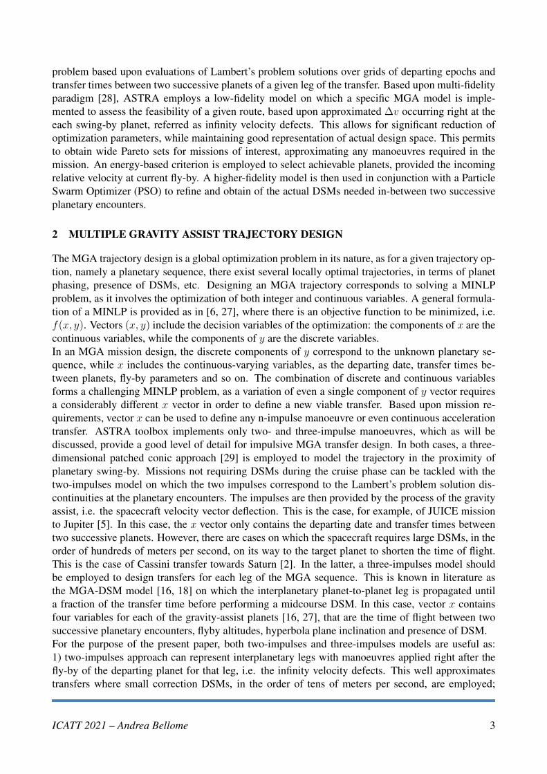
Figure 1: ASTRA multi-fidelity approach to MGA mission design.

Figure 1 shows how the two models, associated to different fidelities, are employed in ASTRA main

engine. In the low-fidelity process, ASTRA employs the two-impulses model coupled with heuristic

strategies (see also later section 3.1.1) to automatically construct MGA sequences. Then, in the high-

fidelity block, ASTRA post-processes the obtained results via direct optimization of solutions coming

from the low-fidelity block, by optimally replacing the defects with mid-course DSMs in between

two successive planetary encounters. A further option in utilisation of multi-fidelity methods is the

use of simplifications in the mathematical models of planetary motion in the first of the two stage

optimisation processes, such as circular co-planar orbits. This option can potentially lead to efficient

problem solutions because of the inherent simplifications that the first approximation may allow. A

potential difficulty arises from the transition to Process 2 where a non-coplanar planetary model is

used to generate real world transfers. In this second model, planetary velocity components can vary

significantly from the circular case. This difficulty is avoided here by using the same planetary model

in both processes.

2.1 Two-impulses model

The lower-fidelity MGA transfer description is based upon successive Lambert arcs connecting two

consecutive swing-bys, e.g. in STOUR [23, 24, 25]. The cost of an MGA leg (without midcourse

DSMs) could be either approximated by a powered fly-by or by a small manoeuvre applied after the

first planet of the leg. A powered fly-by model assumes a ∆v manoeuvre at the pericentre of the

incoming swing-by hyperbola to match the incoming and outgoing spacecraft velocities. However,

this method has not been implemented in the context of real interplanetary missions, due to navigation

challenges that it arises. Therefore, ∆v on each leg of the MGA sequence are computed as defects

between incoming and outgoing spacecraft relative velocity with respect to the planet, which are

solutions of Lambert’s problem for the given leg. These velocity discontinuities between legs are thus

considered as impulsive manoeuvres applied right after the planetary encounter.

The change of direction between incoming and outgoing legs of the fly-by is computed through the

angle δ, such that cos(δ) = ~v−∞·~v+∞|~v−∞||~v+∞|

, where ~v−∞ and ~v+∞ are the spacecraft relative velocity with respect

to the flyby planet (also called infinity velocities). Superscripts − and + are used to describe incoming

and outgoing variables, respectively. Angle δ is then found from the inverse cosine with a positive

ICATT 2021 – Andrea Bellome 4

180-degree range. The maximum deflection is limited by the periapsis of the fly-by hyperbola rp

through: δmax = 2asin([1 +rp,min|~v

−

∞|2

µpl]−1), where rp,min is the the minimum allowable periapsis and

µpl is the gravitational parameter of the fly-by planet (see also section 3.2). Discontinuities between

~v−∞ and ~v+∞, which we call infinity velocity defects, are then compensated through a ∆v computed

immediately after the fly-by [30]:

∆v =

{

||~v+∞| − |~v−∞||, if δ ≤ δmax√

|~v+∞|2 + |~v−∞|2 − |~v+∞||~v−∞| cos (δmax − δ), otherwise

Note that since ~v−∞ and ~v+∞ represent spacecraft velocities relative to the fly-by body, the ∆v ultimately

depends upon planet ephemerides, through its heliocentric velocity at the encounter epoch. Therefore,

vector x, in its low-fidelity representation, only contains the departing epoch t0 and the time of flight

(TOF ) for all the legs (i.e. x = [t0, TOF1, ..., TOFn−1], where n is the number of planets in the

sequence). The cost f(x, y) is then typically written as:

f(x, y) = |~v∞,dep|+n−2∑

i=1

∆vi + |~v∞,arr| (1)

where ~v∞,dep and ~v∞,arr are the infinity velocities relative to the departing and arrival planet of the

entire MGA sequence, respectively (no ∆v is assumed on the first leg of the transfer).

2.2 Three-impulses model

The three impulses model, also called MGA-DSM model, is a well-known approach to tackle op-

timization of MGA transfers [16, 18] with regards to continuous-varying variables contained in xvector. In the MGA-DSM model, an impulsive manoeuvre is used to replace the infinity velocity de-

fect at the first planetary encounter of a given leg. The DSM is computed as a velocity discontinuity

applied after a fraction k of the time of flight TOF of a given leg. The next planet is then targeted with

a solution of Lambert’s problem and the DSMs is derived. Therefore, each flyby is now characterized

by |~v−∞| = |~v+∞| where:

~v+∞ = ~v−∞[cos δb1 + sin ζ sin δb2 + cos ζ sin δb3] (2)

on which: δ is the deflection angle, ζ describes the rotation of the relative velocity through the in-

clination of the fly-by hyperbola in planetary reference frame. Vectors b1, b2 and b3 are the b-plane

unit vectors and are defined as: b1 = ~v−∞/|~v−∞|, b2 = (b1 × ~ri)/|~ri| (~ri being the position vector of the

fly-by planet), and b3 = b2 × b1 (see also [31]). Thus, the number of decision variables is increased

by three (i.e. rp, k and ζ ) for each planetary encounter, compared to the two-impulses model.

ICATT 2021 – Andrea Bellome 5

3 BUILDING THE ROUTE SET IN ASTRA

ASTRA employs a multi-fidelity approach to automatically solving the MGA problem. The pipeline

consists in two successive processes (see also Figure 1): 1) Process 1: Automatic MGA sequence

construction; 2) Process 2: Route refinement and post-processing.

The low-fidelity Process 1 allows to generate a list of successive possible encounters with Solar Sys-

tem planets, by means of energetic considerations at current planetary swing-by. Transfer options

towards identified planets are then evaluated by successively solving Lambert’s problem over a grid

of arrival dates at next planet encounter. A two-impulses model as described in section 2.1 is used

to compute the ∆v defects. This process is repeated until the target planet is reached. In the higher-

fidelity Process 2, ASTRA orders all the routes constructed in previous steps according to a ranking

criterion, which typically is the cost expressed in equation 1, or the total transfer time, or a combina-

tion thereof. Moreover, fly-by parameters (rp, ζ) are obtained for all the swing-bys in the sequences,

and ultimately the ∆v defects are replaced by mid-course DSMs between two successive planetary

encounters via refinement optimization using the MGA-DSM model described in section 2.2.

3.1 Process 1: Automatic MGA sequence construction

Algorithm 1 Building the route set in ASTRA’s Process 1 with two-impulses low-fidelity model.

1: Select departing and target planets and departing date range

2: for each departing date do

3: while the target planet is not reached do

4: check the achievable planets

5: for each planet identified do

6: Lambert arc transfer exploration for the range of feasible transfer times

7: compute the defects

8: end

9: apply filtering criteria ⊲ see section 3.1.1

10: end while

11: end

Algorithm 1 illustrates the main systematic search process implemented in ASTRA’s low-fidelity

Process 1. The process requires first to identify the departure and target (final) planet, as well as the

discretised launch window (i.e.,vector of start or departure dates). At the start of each successive leg

(i.e., line 4 in Algorithm 1), a swing-by assessment step is needed to generate the list of successive

reachable planets. Thus, the outgoing relative velocity vectors that maximises and minimises the

energy of the spacecraft at departure of the current planet are calculated and used to assessed the

planets that can be crossed and, so, potentially reached. Figure 2 depicts this process for all legs,

other than the departure leg, where the outgoing relative velocity at the departing planet |~v∞,dep| can

be defined instead by the launcher capability.

Figure 2 assumed that incoming relative velocity ~v−∞ is deflected by the angle δ such that the closest

possible alignment with the gravity-assist body velocity ~vga is achieved post swing-by. If minimum

pericentre allows the relative velocity vector post swing-by ~v+∞ would become aligned with −~vga or

~vga, i.e. minimizing or maximizing energy. Therefore, after the swing-by, the spacecraft heliocentric

velocity ~v+sc would be ~v+sc = −|~v−∞|~vga/|~vga| or ~v+sc = |~v−∞|~vga/|~vga| only if α + δmax ≥ 180o (in-front

passage), or α − δmax ≤ 0o (behind passage), respectively (see Figure 2). The angle α (positive in

180-degree range ) can be computed from geometry from Figure 2 as α = acos( ~v−∞·~vga

|~v−∞||~vga|).

ICATT 2021 – Andrea Bellome 6

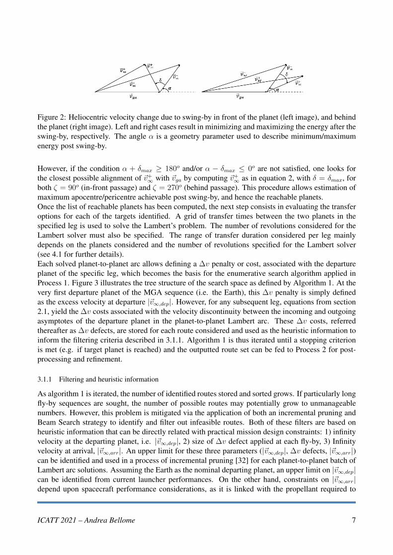
Figure 2: Heliocentric velocity change due to swing-by in front of the planet (left image), and behind

the planet (right image). Left and right cases result in minimizing and maximizing the energy after the

swing-by, respectively. The angle α is a geometry parameter used to describe minimum/maximum

energy post swing-by.

However, if the condition α + δmax ≥ 180o and/or α − δmax ≤ 0o are not satisfied, one looks for

the closest possible alignment of ~v+∞ with ~vga by computing ~v+∞ as in equation 2, with δ = δmax, for

both ζ = 90o (in-front passage) and ζ = 270o (behind passage). This procedure allows estimation of

maximum apocentre/pericentre achievable post swing-by, and hence the reachable planets.

Once the list of reachable planets has been computed, the next step consists in evaluating the transfer

options for each of the targets identified. A grid of transfer times between the two planets in the

specified leg is used to solve the Lambert’s problem. The number of revolutions considered for the

Lambert solver must also be specified. The range of transfer duration considered per leg mainly

depends on the planets considered and the number of revolutions specified for the Lambert solver

(see 4.1 for further details).

Each solved planet-to-planet arc allows defining a ∆v penalty or cost, associated with the departure

planet of the specific leg, which becomes the basis for the enumerative search algorithm applied in

Process 1. Figure 3 illustrates the tree structure of the search space as defined by Algorithm 1. At the

very first departure planet of the MGA sequence (i.e. the Earth), this ∆v penalty is simply defined

as the excess velocity at departure |~v∞,dep|. However, for any subsequent leg, equations from section

2.1, yield the ∆v costs associated with the velocity discontinuity between the incoming and outgoing

asymptotes of the departure planet in the planet-to-planet Lambert arc. These ∆v costs, referred

thereafter as ∆v defects, are stored for each route considered and used as the heuristic information to

inform the filtering criteria described in 3.1.1. Algorithm 1 is thus iterated until a stopping criterion

is met (e.g. if target planet is reached) and the outputted route set can be fed to Process 2 for post-

processing and refinement.

3.1.1 Filtering and heuristic information

As algorithm 1 is iterated, the number of identified routes stored and sorted grows. If particularly long

fly-by sequences are sought, the number of possible routes may potentially grow to unmanageable

numbers. However, this problem is mitigated via the application of both an incremental pruning and

Beam Search strategy to identify and filter out infeasible routes. Both of these filters are based on

heuristic information that can be directly related with practical mission design constraints: 1) infinity

velocity at the departing planet, i.e. |~v∞,dep|, 2) size of ∆v defect applied at each fly-by, 3) Infinity

velocity at arrival, |~v∞,arr|. An upper limit for these three parameters (|~v∞,dep|, ∆v defects, |~v∞,arr|)can be identified and used in a process of incremental pruning [32] for each planet-to-planet batch of

Lambert arc solutions. Assuming the Earth as the nominal departing planet, an upper limit on |~v∞,dep|can be identified from current launcher performances. On the other hand, constraints on |~v∞,arr|depend upon spacecraft performance considerations, as it is linked with the propellant required to

ICATT 2021 – Andrea Bellome 7

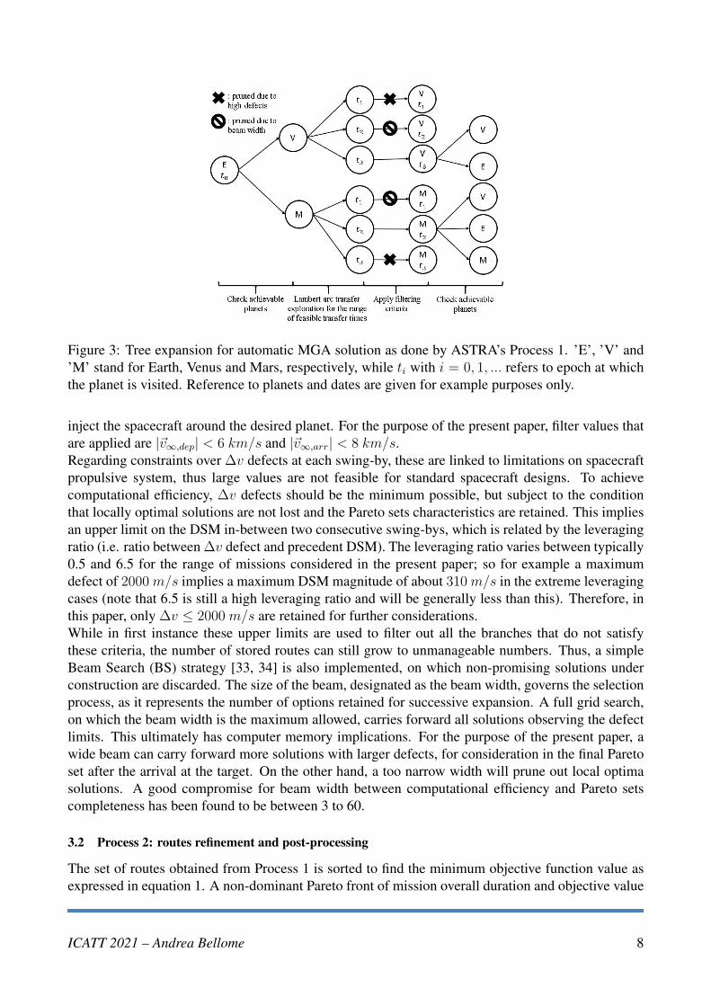
Figure 3: Tree expansion for automatic MGA solution as done by ASTRA’s Process 1. ’E’, ’V’ and

’M’ stand for Earth, Venus and Mars, respectively, while ti with i = 0, 1, ... refers to epoch at which

the planet is visited. Reference to planets and dates are given for example purposes only.

inject the spacecraft around the desired planet. For the purpose of the present paper, filter values that

are applied are |~v∞,dep| < 6 km/s and |~v∞,arr| < 8 km/s.

Regarding constraints over ∆v defects at each swing-by, these are linked to limitations on spacecraft

propulsive system, thus large values are not feasible for standard spacecraft designs. To achieve

computational efficiency, ∆v defects should be the minimum possible, but subject to the condition

that locally optimal solutions are not lost and the Pareto sets characteristics are retained. This implies

an upper limit on the DSM in-between two consecutive swing-bys, which is related by the leveraging

ratio (i.e. ratio between ∆v defect and precedent DSM). The leveraging ratio varies between typically

0.5 and 6.5 for the range of missions considered in the present paper; so for example a maximum

defect of 2000m/s implies a maximum DSM magnitude of about 310m/s in the extreme leveraging

cases (note that 6.5 is still a high leveraging ratio and will be generally less than this). Therefore, in

this paper, only ∆v ≤ 2000 m/s are retained for further considerations.

While in first instance these upper limits are used to filter out all the branches that do not satisfy

these criteria, the number of stored routes can still grow to unmanageable numbers. Thus, a simple

Beam Search (BS) strategy [33, 34] is also implemented, on which non-promising solutions under

construction are discarded. The size of the beam, designated as the beam width, governs the selection

process, as it represents the number of options retained for successive expansion. A full grid search,

on which the beam width is the maximum allowed, carries forward all solutions observing the defect

limits. This ultimately has computer memory implications. For the purpose of the present paper, a

wide beam can carry forward more solutions with larger defects, for consideration in the final Pareto

set after the arrival at the target. On the other hand, a too narrow width will prune out local optima

solutions. A good compromise for beam width between computational efficiency and Pareto sets

completeness has been found to be between 3 to 60.

3.2 Process 2: routes refinement and post-processing

The set of routes obtained from Process 1 is sorted to find the minimum objective function value as

expressed in equation 1. A non-dominant Pareto front of mission overall duration and objective value

ICATT 2021 – Andrea Bellome 8

can then be derived. Pareto fronts are computed based on the ∆v defects as computed in equations

from section 2.1. However, ∆v defects are manoeuvres applied immediately after departure from a

fly-by and so they do not represent real manoeuvres in the context of a mission design. Therefore

in ASTRA, as a post-processing stage, after results are obtained and sorted, these ∆v defects are

converted to DSMs between two successive planets in the sequence. This is done employing the

MGA-DSM three-impulses model described in section 2.2.

As first step of post-processing stage, fly-by parameters rp and ζ need to be derived. For each swing-

by encounter, Process 1 has provided ~v−∞ and ~v+∞, as well as the encounter epochs. Therefore, similarly

as already done in section 2.1, one computes if the ∆v defect can be compensated with the gravity

of the current fly-by body or not, checking if δ ≤ δmax. If the condition is satisfied, then an rpexists such that the infinity velocity post fly-by is |~v−∞|~v+∞/|~v+∞|. In this case, the eccentricity e and

semi-major axis a of the fly-by hyperbola are: e = [sin δ2]−1 and a = −

µpl

|~v−∞|2. Where µpl is the

gravitational parameter of the fly-by body. Therefore, the periapsis radius is: rp = a(1−e). However,

if the condition δ ≤ δmax is not satisfied, one assumes the maximum deflection fly-by defined by

rp = rp,min. For the purposes of the present paper, a minimum altitude of 200 km is considered for

Venus, Earth and Mars fly-bys. Once rp and thus δ are known, one can compute the fly-by angle ζ by

inverting equation 2. One computes the vector ~w = [w1, w2, w3]T = [cos δ, sin ζ sin δ, cos ζ sin δ]T as

~w = 1

|~v+∞|M−1~v+∞. Where the matrix M = [b1, b2, b3] is found from the definition of b1, b2 and b3 as

described in section 2.2. Finally, one has ζ = arctan(w2/w3), positive in the 360-degrees range.

As second step of post-processing stage, the ∆v defects need to be replaced with DSMs occurring

after a fraction of the transfer time between two consecutive swing-bys, according to the MGA-DSM

model provided in section 2.2. ASTRA employs Particle Swarm Optimization (PSO) [35], [36] to

look for the optimal location of DSM along the given leg of the transfer. The optimiser is initialised

using solutions from Process 1, and derived fly-by parameters and time intervals are used to derive

control inputs for the full optimiser. Such an optimization efficiently converges to the solution (see

4.1 ), eliminating defects and inserting DSMs where optimal.

4 CASE STUDIES

Optimal transfers are determined for benchmark missions to test the performances of ASTRA solver.

An MGA mission towards Jupiter is tested referring to European Space Agency (ESA)’s JUICE mis-

sion [5], due to launch in 2022. JUICE is intended to follow the sequence Earth-Earth-Venus-Earth-

Mars-Earth-Jupiter (the first planet being the departing one).

4.1 Missions towards Jupiter

Transfers towards Jupiter are explored for a departure date in 2023. This allows to benchmark AS-

TRA solutions with those proposed by the ESA’s mission JUICE [5]. Note that JUICE departure

from Earth is set in 2022 and its first gravity assisted manoeuvre is also at Earth in May 2023. The

spacecraft will then encounter Venus, Earth, Mars, and Earth again to increase its energy, resulting

in an EEVEMEJ sequence (’E’, ’V’, ’M’ and ’J’ stand for ’Earth’, ’Venus’, ’Mars’ and ’Jupiter’,

respectively). However, the first leg of the mission is a one-year Earth resonant transfer whose main

function is to allow a plane change at the Earth fly-by to swing the orbit plane close to the ecliptic.

ASTRA, as a preliminary trajectory design tool, does not implement considerations on the available

declinations of the Earth departure asymptote. Therefore, in order to appropriately benchmark the

published trajectories for JUICE mission, a departure in 2023 is considered instead. The full 2023

launch window is explored, with departing dates separated by steps of 10 days.

ICATT 2021 – Andrea Bellome 9

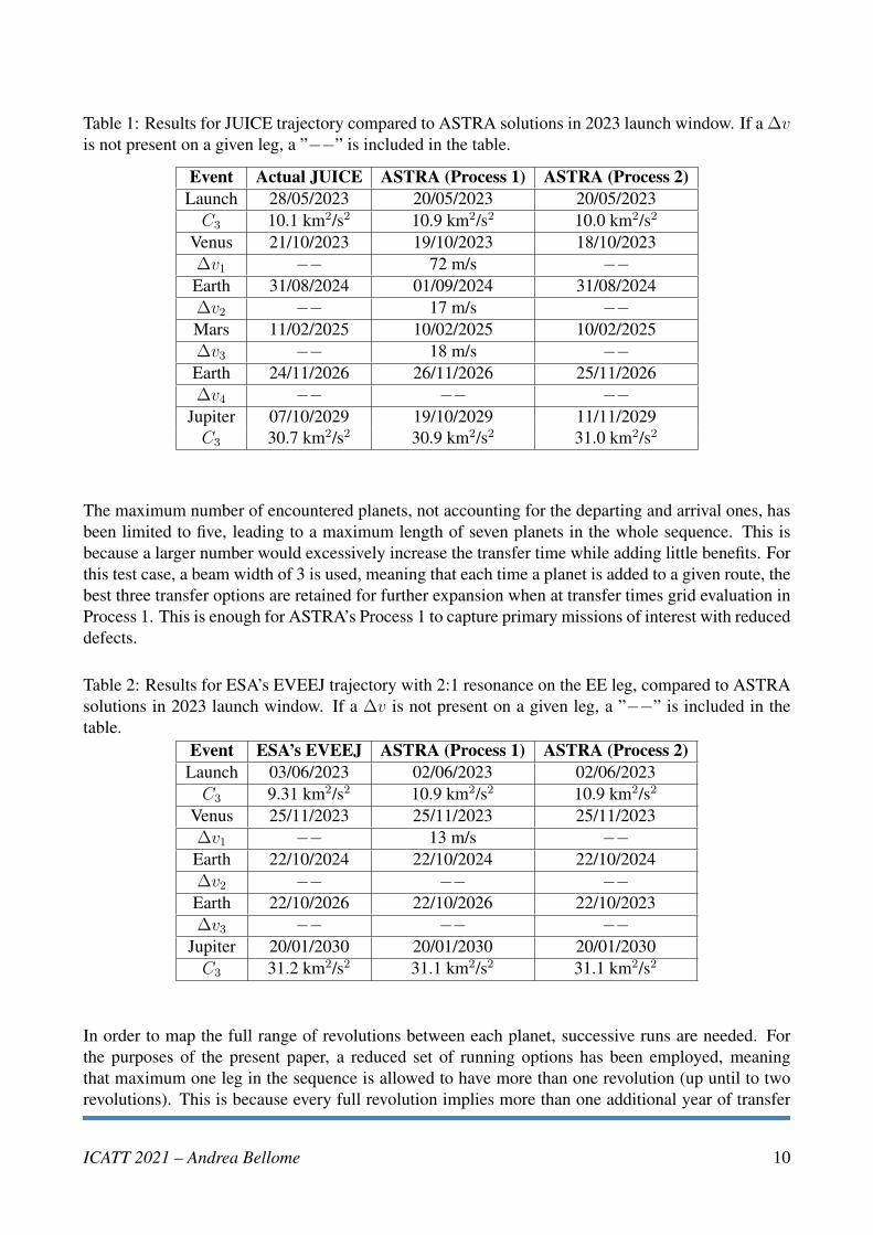
Table 1: Results for JUICE trajectory compared to ASTRA solutions in 2023 launch window. If a ∆vis not present on a given leg, a ”−−” is included in the table.

Event Actual JUICE ASTRA (Process 1) ASTRA (Process 2)

Launch 28/05/2023 20/05/2023 20/05/2023

C3 10.1 km2/s2 10.9 km2/s2 10.0 km2/s2

Venus 21/10/2023 19/10/2023 18/10/2023

∆v1 −− 72 m/s −−Earth 31/08/2024 01/09/2024 31/08/2024

∆v2 −− 17 m/s −−Mars 11/02/2025 10/02/2025 10/02/2025

∆v3 −− 18 m/s −−Earth 24/11/2026 26/11/2026 25/11/2026

∆v4 −− −− −−Jupiter 07/10/2029 19/10/2029 11/11/2029

C3 30.7 km2/s2 30.9 km2/s2 31.0 km2/s2

The maximum number of encountered planets, not accounting for the departing and arrival ones, has

been limited to five, leading to a maximum length of seven planets in the whole sequence. This is

because a larger number would excessively increase the transfer time while adding little benefits. For

this test case, a beam width of 3 is used, meaning that each time a planet is added to a given route, the

best three transfer options are retained for further expansion when at transfer times grid evaluation in

Process 1. This is enough for ASTRA’s Process 1 to capture primary missions of interest with reduced

defects.

Table 2: Results for ESA’s EVEEJ trajectory with 2:1 resonance on the EE leg, compared to ASTRA

solutions in 2023 launch window. If a ∆v is not present on a given leg, a ”−−” is included in the

table.

Event ESA’s EVEEJ ASTRA (Process 1) ASTRA (Process 2)

Launch 03/06/2023 02/06/2023 02/06/2023

C3 9.31 km2/s2 10.9 km2/s2 10.9 km2/s2

Venus 25/11/2023 25/11/2023 25/11/2023

∆v1 −− 13 m/s −−Earth 22/10/2024 22/10/2024 22/10/2024

∆v2 −− −− −−Earth 22/10/2026 22/10/2026 22/10/2023

∆v3 −− −− −−Jupiter 20/01/2030 20/01/2030 20/01/2030

C3 31.2 km2/s2 31.1 km2/s2 31.1 km2/s2

In order to map the full range of revolutions between each planet, successive runs are needed. For

the purposes of the present paper, a reduced set of running options has been employed, meaning

that maximum one leg in the sequence is allowed to have more than one revolution (up until to two

revolutions). This is because every full revolution implies more than one additional year of transfer

ICATT 2021 – Andrea Bellome 10

time, thus increasing the total time of flight considerably. Moreover, the main aim of ASTRA is to

assess the feasibility of finding promising encounters. However, this reduction of transfer options still

allows to identify primary missions of interest for the Jupiter case.

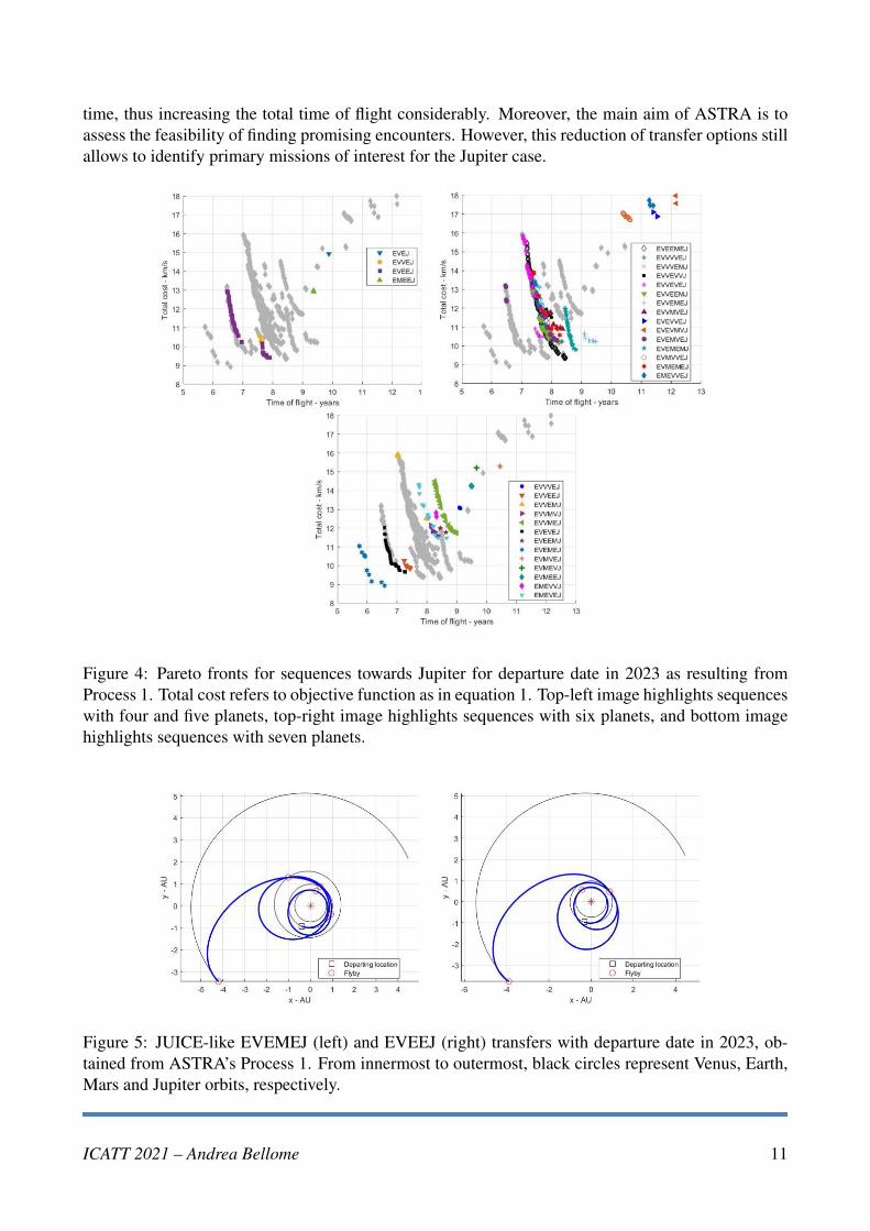
Figure 4: Pareto fronts for sequences towards Jupiter for departure date in 2023 as resulting from

Process 1. Total cost refers to objective function as in equation 1. Top-left image highlights sequences

with four and five planets, top-right image highlights sequences with six planets, and bottom image

highlights sequences with seven planets.

Figure 5: JUICE-like EVEMEJ (left) and EVEEJ (right) transfers with departure date in 2023, ob-

tained from ASTRA’s Process 1. From innermost to outermost, black circles represent Venus, Earth,

Mars and Jupiter orbits, respectively.

ICATT 2021 – Andrea Bellome 11

Pareto sets of available transfer opportunities as resulting from Process 1 of ASTRA search are shown

in Figure 4. As expected, among the sequences, the EVEMEJ is found to be the optimal one, i.e. the

one with lowest total cost and transfer time. Note that also the well-known sequence EVEEJ performs

well in 2023 launch window, provided the 2:1 resonance between the consecutive Earth swing-bys

(note that resonant transfers are computed separately from main search engine as in Algorithm 1 and

following the procedure found in [15]). Details of EVEMEJ and EVEEJ sequences, compared to

actual JUICE [37] and ESA Red Book 1, are provided in Table 1 and 2. Figure 5 show ecliptic pro-

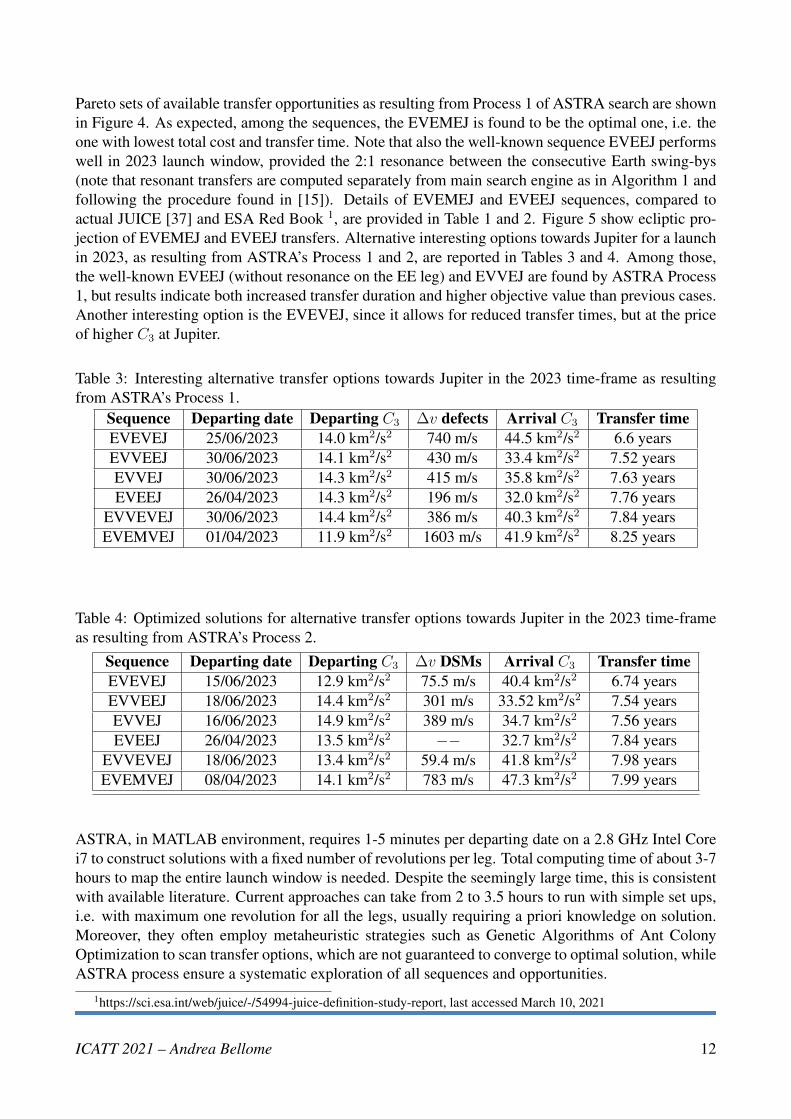
jection of EVEMEJ and EVEEJ transfers. Alternative interesting options towards Jupiter for a launch

in 2023, as resulting from ASTRA’s Process 1 and 2, are reported in Tables 3 and 4. Among those,

the well-known EVEEJ (without resonance on the EE leg) and EVVEJ are found by ASTRA Process

1, but results indicate both increased transfer duration and higher objective value than previous cases.

Another interesting option is the EVEVEJ, since it allows for reduced transfer times, but at the price

of higher C3 at Jupiter.

Table 3: Interesting alternative transfer options towards Jupiter in the 2023 time-frame as resulting

from ASTRA’s Process 1.

Sequence Departing date Departing C3 ∆v defects Arrival C3 Transfer time

EVEVEJ 25/06/2023 14.0 km2/s2 740 m/s 44.5 km2/s2 6.6 years

EVVEEJ 30/06/2023 14.1 km2/s2 430 m/s 33.4 km2/s2 7.52 years

EVVEJ 30/06/2023 14.3 km2/s2 415 m/s 35.8 km2/s2 7.63 years

EVEEJ 26/04/2023 14.3 km2/s2 196 m/s 32.0 km2/s2 7.76 years

EVVEVEJ 30/06/2023 14.4 km2/s2 386 m/s 40.3 km2/s2 7.84 years

EVEMVEJ 01/04/2023 11.9 km2/s2 1603 m/s 41.9 km2/s2 8.25 years

Table 4: Optimized solutions for alternative transfer options towards Jupiter in the 2023 time-frame

as resulting from ASTRA’s Process 2.

Sequence Departing date Departing C3 ∆v DSMs Arrival C3 Transfer time

EVEVEJ 15/06/2023 12.9 km2/s2 75.5 m/s 40.4 km2/s2 6.74 years

EVVEEJ 18/06/2023 14.4 km2/s2 301 m/s 33.52 km2/s2 7.54 years

EVVEJ 16/06/2023 14.9 km2/s2 389 m/s 34.7 km2/s2 7.56 years

EVEEJ 26/04/2023 13.5 km2/s2 −− 32.7 km2/s2 7.84 years

EVVEVEJ 18/06/2023 13.4 km2/s2 59.4 m/s 41.8 km2/s2 7.98 years

EVEMVEJ 08/04/2023 14.1 km2/s2 783 m/s 47.3 km2/s2 7.99 years

ASTRA, in MATLAB environment, requires 1-5 minutes per departing date on a 2.8 GHz Intel Core

i7 to construct solutions with a fixed number of revolutions per leg. Total computing time of about 3-7

hours to map the entire launch window is needed. Despite the seemingly large time, this is consistent

with available literature. Current approaches can take from 2 to 3.5 hours to run with simple set ups,

i.e. with maximum one revolution for all the legs, usually requiring a priori knowledge on solution.

Moreover, they often employ metaheuristic strategies such as Genetic Algorithms of Ant Colony

Optimization to scan transfer options, which are not guaranteed to converge to optimal solution, while

ASTRA process ensure a systematic exploration of all sequences and opportunities.

1https://sci.esa.int/web/juice/-/54994-juice-definition-study-report, last accessed March 10, 2021

ICATT 2021 – Andrea Bellome 12

5 CONCLUSIONS

This paper presents an efficient approach to solve on a quasi-systematic manner the automatic MGA

problem. The search is systematic as in the sense that is performed for all possible combinations of

planet-to-planet transfers and for a thick grid of departure conditions and time of flights for all legs.

Such an approach is made possible through a multi-fidelity model of the planet-to-planet transfer,

on which on its low-fidelity set up is modelled as a planet-to-planet Lambert arc, where all velocity

discontinuities are considered as ∆v penalties on the fitness function.

Yet, the complete exploration of all possible combination of planet-to-planet transfers and all pos-

sible combination of departure and arrival times would be a rather inefficient and computationally

cumbersome task. Thus, a filtering process is used for every planet-to-planet combination in order to

limit the growth of solutions to only reasonably feasible transfers. This method has proven to be effi-

cient and effective in identifying primary sequences of interest for Jupiter and Saturn mission cases,

by performing grid scans of possible planetary encounters and employing a reduced set of control

parameters, maintaining good representation of the search space.

Compared to existing approaches, while employing similar computational efforts, ASTRA does not

need a priori knowledge of the solution (e.g. on the departing date or velocity) and it is comprehensive

in that it automatically considers all feasible planetary fly-by sequences. Moreover, by approximating

the DSMs as infinity velocity defects at each planetary encounter, ASTRA is able to generate wide

sets of solutions to represent broad Pareto sets useful for preliminary mission analysis.

The key aspect of this approach is therefore the specific multi-fidelity process used, in considering

two- and three-impulse transfers and the inclusion of all feasible planet fly-by sequences in any given

transfer problem. The transition between processes here is facilitated by the use of the general eccen-

tric 3D planetary motions in both processes of the optimisation.

Future releases of ASTRA will include grid search approach hybridized with tree-like metaheuristic

strategies, such as Ant Colony Optimization (ACO), to increase computational efficiency, without

scarifying the convergence to global optima solutions. Moreover, future research will also focus on

mapping the swing-by discontinuities (i.e. ∆v defects) into actual Deep Space Manoeuvres (DSMs)

while in the search steps, maintaining efficient computational efforts.

REFERENCES

[1] L. A. D’Amario, D. V. Byrnes, J. R. Johannesen, and B. G. Nolan, “Galileo 1989 VEEGA

trajectory design,” Journal of the Astronautical Sciences, vol. 37, pp. 281–306, 1989.

[2] F. Peralta and S. Flanagan, “Cassini interplanetary trajectory design,” Control Engineering Prac-

tice, vol. 3, no. 11, pp. 1603–1610, 1995.

[3] D. G. Yarnoz, R. Jehn, and M. Croon, “Interplanetary navigation along the low-thrust trajectory

of bepicolombo,” Acta Astronautica, vol. 59, no. 1-5, pp. 284–293, 2006.

[4] J. Sanchez Perez, W. Martens, and G. Varga, “Solar orbiter 2020 february mission profile,”

Advances in the Astronautical Sciences, vol. 167, p. 1395–1410, 2018.

[5] O. Grasset, M. K. Dougherty, A. Coustenis, E. J. Bunce, C. Erd, D. Titov, M. Blanc, A. Coates,

P. Drossart, and L. N. Fletcher, “JUpiter ICy moons Explorer (JUICE): An ESA mission to orbit

Ganymede and to characterise the Jupiter system,” Planetary and Space Science, vol. 78, pp.

1–21, 2013.

ICATT 2021 – Andrea Bellome 13

[6] M. Schlueter, S. O. Erb, M. Gerdts, S. Kemble, and J.-J. Ruckmann, “Midaco on minlp space

applications,” Advances in Space Research, vol. 51, no. 7, pp. 1116–1131, 2013.

[7] I. M. Ross and C. N. D’Souza, “Hybrid optimal control framework for mission planning,” Jour-

nal of Guidance, Control, and Dynamics, vol. 28, no. 4, pp. 686–697, 2005.

[8] C. M. Chilan and B. A. Conway, “A space mission automaton using hybrid optimal control,” in

17th Annual Space Flight Mechanics Meeting, 2007, pp. 259–276.

[9] B. J. Wall and B. A. Conway, “Genetic algorithms applied to the solution of hybrid optimal

control problems in astrodynamics,” Journal of Global Optimization, vol. 44, no. 4, p. 493,

2009.

[10] J. A. Englander, B. A. Conway, and T. Williams, “Automated mission planning via evolutionary

algorithms,” Journal of Guidance, Control, and Dynamics, vol. 35, no. 6, pp. 1878–1887, 2012.

[11] J. Englander, B. Conway, and T. Williams, “Automated interplanetary trajectory planning,” in

AIAA/AAS Astrodynamics Specialist Conference, 2012, p. 4517.

[12] M. Ceriotti and M. Vasile, “MGA trajectory planning with an ACO-inspired algorithm,” Acta

Astronautica, vol. 67, no. 9-10, pp. 1202–1217, 2010.

[13] A. Gad and O. Abdelkhalik, “Hidden genes genetic algorithm for multi-gravity-assist trajecto-

ries optimization,” Journal of Spacecraft and Rockets, vol. 48, no. 4, pp. 629–641, 2011.

[14] O. Abdelkhalik and A. Gad, “Dynamic-size multiple populations genetic algorithm for

multigravity-assist trajectory optimization,” Journal of Guidance, Control, and Dynamics,

vol. 35, no. 2, pp. 520–529, 2012.

[15] S. Wagner and B. Wie, “Hybrid algorithm for multiple gravity-assist and impulsive delta-V

maneuvers,” Journal of Guidance, Control, and Dynamics, vol. 38, no. 11, pp. 2096–2107,

2015.

[16] M. Vasile and P. De Pascale, “Preliminary design of multiple gravity-assist trajectories,” Journal

of Spacecraft and Rockets, vol. 43, no. 4, pp. 794–805, 2006.

[17] N. Strange and J. Longuski, “Graphical method for gravity-assist trajectory design,” J. Spacecr.

Rockets, vol. 37, p. 9–16, 2002.

[18] T. Vinko and D. Izzo, “Global optimisation heuristics and test problems for preliminary space-

craft trajectory design,” Advanced Concepts Team, ESATR ACT-TNT-MAD-GOHTPPSTD, Sept,

2008.

[19] M. Pontani and B. A. Conway, “Particle swarm optimization applied to space trajectories,” Jour-

nal of Guidance, Control, and Dynamics, vol. 33, no. 5, pp. 1429–1441, 2010.

[20] M. Vasile, E. Minisci, and M. Locatelli, “Analysis of some global optimization algorithms for

space trajectory design,” Journal of Spacecraft and Rockets, vol. 47, no. 2, pp. 334–344, 2010.

[21] M. Schlueter, “Nonlinear mixed integer based optimization technique for space applications,”

2012.

ICATT 2021 – Andrea Bellome 14

[22] A. D. Olds, C. A. Kluever, and M. L. Cupples, “Interplanetary mission design using differential

evolution,” Journal of Spacecraft and Rockets, vol. 44, no. 5, pp. 1060–1070, 2007.

[23] J. M. Longuski and S. N. Williams, “Automated design of gravity-assist trajectories to mars and

the outer planets,” Celestial Mechanics and Dynamical Astronomy, vol. 52, no. 3, pp. 207–220,

1991.

[24] J. A. Sims, A. J. Staugler, and J. M. Longuski, “Trajectory options to pluto via gravity assists

from venus, mars, and jupiter,” Journal of Spacecraft and Rockets, vol. 34, no. 3, pp. 347–353,

1997.

[25] A. E. Petropoulos, J. M. Longuski, and E. P. Bonfiglio, “Trajectories to jupiter via gravity assists

from venus, earth, and mars,” Journal of Spacecraft and Rockets, vol. 37, no. 6, pp. 776–783,

2000.

[26] D. Izzo, V. M. Becerra, D. R. Myatt, S. J. Nasuto, and J. M. Bishop, “Search space pruning

and global optimisation of multiple gravity assist spacecraft trajectories,” Journal of Global

Optimization, vol. 38, no. 2, pp. 283–296, 2007.

[27] A. Bellome, J.-P. S. Cuartielles, L. Felicetti, and S. Kemble, “Modified tisserand map exploration

for preliminary multiple gravity assist trajectory design,” 2020.

[28] B. Peherstorfer, K. Willcox, and M. Gunzburger, “Survey of multifidelity methods in uncertainty

propagation, inference, and optimization,” Siam Review, vol. 60, no. 3, pp. 550–591, 2018.

[29] M. A. Minovitch, “The invention that opened the solar system to exploration,” Planetary and

Space Science, vol. 58, no. 6, pp. 885–892, 2010.

[30] M. Lavagna, A. Povoleri, and A. Finzi, “Interplanetary mission design with aero-assisted ma-

noeuvres multi-objective evolutive optimization,” Acta Astronautica, vol. 57, no. 2-8, pp. 498–

509, 2005.

[31] D. Izzo, “Advances in global optimisation for space trajectory design,” in Proceedings of the

international symposium on space technology and science, vol. 25, 2006, p. 563.

[32] M. Vasile, M. Ceriotti, V. M. Becerra, and S. Nasuto, “An incremental algorithm for the op-

timization of multiple gravity assist trajectories,” in Computational intelligence in aerospace

sciences. American Institute of Aeronautics and Astronautics, 2014, pp. 745–779.

[33] S. C. Shapiro, Encyclopedia of artificial intelligence second edition. John Wiley and Sons,

Inc., 1987.

[34] C. M. Wilt, J. T. Thayer, and W. Ruml, “A comparison of greedy search algorithms,” in Third

Annual Symposium on Combinatorial Search, 2010, pp. 129–136.

[35] R. Eberhart and J. Kennedy, “A new optimizer using particle swarm theory,” in MHS’95. Pro-

ceedings of the Sixth International Symposium on Micro Machine and Human Science. Ieee,

1995, pp. 39–43.

[36] J. Kennedy and R. Eberhart, “Particle swarm optimization,” in Proceedings of ICNN’95-

international conference on neural networks, vol. 4. IEEE, 1995, pp. 1942–1948.

[37] E. Ecale, F. Torelli, and I. Tanco, “Juice interplanetary operations design: drivers and chal-

lenges,” in 2018 SpaceOps Conference, 2018, p. 2493.

ICATT 2021 – Andrea Bellome 15