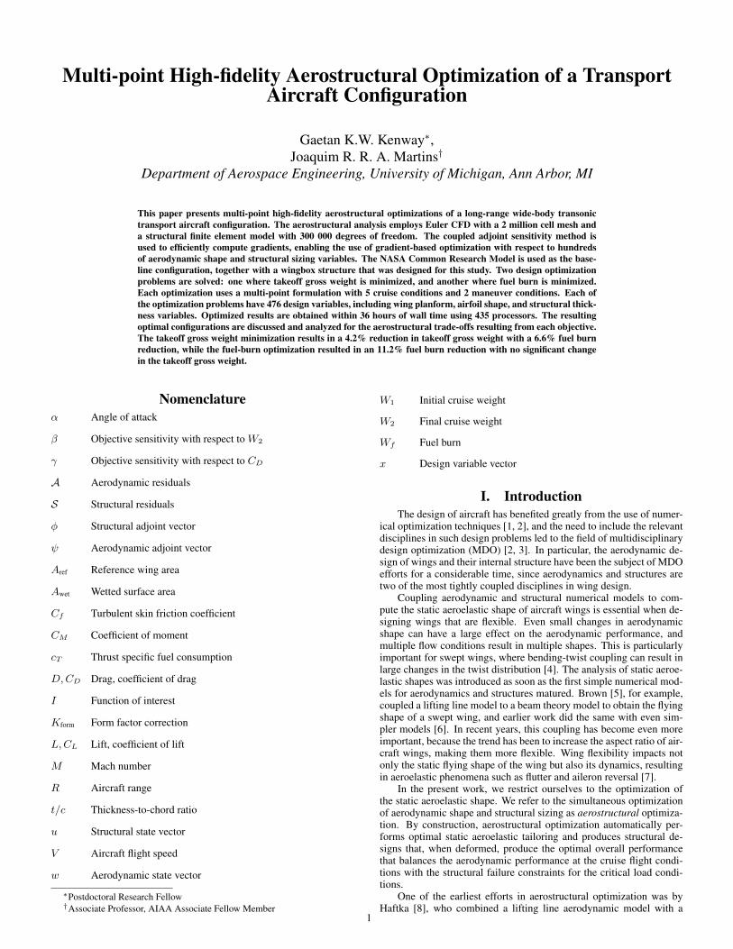
Multi-point High-fidelity Aerostructural Optimization of a TransportAircraft Configuration

Gaetan K.W. Kenway∗,Joaquim R. R. A. Martins†

Department of Aerospace Engineering, University of Michigan, Ann Arbor, MI

This paper presents multi-point high-fidelity aerostructural optimizations of a long-range wide-body transonictransport aircraft configuration. The aerostructural analysis employs Euler CFD with a 2 million cell mesh anda structural finite element model with 300 000 degrees of freedom. The coupled adjoint sensitivity method isused to efficiently compute gradients, enabling the use of gradient-based optimization with respect to hundredsof aerodynamic shape and structural sizing variables. The NASA Common Research Model is used as the base-line configuration, together with a wingbox structure that was designed for this study. Two design optimizationproblems are solved: one where takeoff gross weight is minimized, and another where fuel burn is minimized.Each optimization uses a multi-point formulation with 5 cruise conditions and 2 maneuver conditions. Each ofthe optimization problems have 476 design variables, including wing planform, airfoil shape, and structural thick-ness variables. Optimized results are obtained within 36 hours of wall time using 435 processors. The resultingoptimal configurations are discussed and analyzed for the aerostructural trade-offs resulting from each objective.The takeoff gross weight minimization results in a 4.2% reduction in takeoff gross weight with a 6.6% fuel burnreduction, while the fuel-burn optimization resulted in an 11.2% fuel burn reduction with no significant changein the takeoff gross weight.

Nomenclatureα Angle of attack

β Objective sensitivity with respect to W2

γ Objective sensitivity with respect to CD

A Aerodynamic residuals

S Structural residuals

φ Structural adjoint vector

ψ Aerodynamic adjoint vector

Aref Reference wing area

Awet Wetted surface area

Cf Turbulent skin friction coefficient

CM Coefficient of moment

cT Thrust specific fuel consumption

D,CD Drag, coefficient of drag

I Function of interest

Kform Form factor correction

L,CL Lift, coefficient of lift

M Mach number

R Aircraft range

t/c Thickness-to-chord ratio

u Structural state vector

V Aircraft flight speed

w Aerodynamic state vector

∗Postdoctoral Research Fellow†Associate Professor, AIAA Associate Fellow Member

W1 Initial cruise weight

W2 Final cruise weight

Wf Fuel burn

x Design variable vector

I. IntroductionThe design of aircraft has benefited greatly from the use of numer-

ical optimization techniques [1, 2], and the need to include the relevantdisciplines in such design problems led to the field of multidisciplinarydesign optimization (MDO) [2, 3]. In particular, the aerodynamic de-sign of wings and their internal structure have been the subject of MDOefforts for a considerable time, since aerodynamics and structures aretwo of the most tightly coupled disciplines in wing design.

Coupling aerodynamic and structural numerical models to com-pute the static aeroelastic shape of aircraft wings is essential when de-signing wings that are flexible. Even small changes in aerodynamicshape can have a large effect on the aerodynamic performance, andmultiple flow conditions result in multiple shapes. This is particularlyimportant for swept wings, where bending-twist coupling can result inlarge changes in the twist distribution [4]. The analysis of static aeroe-lastic shapes was introduced as soon as the first simple numerical mod-els for aerodynamics and structures matured. Brown [5], for example,coupled a lifting line model to a beam theory model to obtain the flyingshape of a swept wing, and earlier work did the same with even sim-pler models [6]. In recent years, this coupling has become even moreimportant, because the trend has been to increase the aspect ratio of air-craft wings, making them more flexible. Wing flexibility impacts notonly the static flying shape of the wing but also its dynamics, resultingin aeroelastic phenomena such as flutter and aileron reversal [7].

In the present work, we restrict ourselves to the optimization ofthe static aeroelastic shape. We refer to the simultaneous optimizationof aerodynamic shape and structural sizing as aerostructural optimiza-tion. By construction, aerostructural optimization automatically per-forms optimal static aeroelastic tailoring and produces structural de-signs that, when deformed, produce the optimal overall performancethat balances the aerodynamic performance at the cruise flight condi-tions with the structural failure constraints for the critical load condi-tions.

One of the earliest efforts in aerostructural optimization was byHaftka [8], who combined a lifting line aerodynamic model with a

1

2

simple structural finite-element analysis to iteratively obtain the fly-ing shape due to the structural deformations. The trade-offs betweenweight and induced drag were quantified for both aluminium and com-posite configurations. Grossman et al. [9] investigated the completeaerostructural analysis and optimization of a sailplane. They showedthat integrated aerostructural optimization gave higher performance de-signs than those found by sequential optimization (aerodynamic op-timization followed by structural minimization). They subsequentlyconsidered the design of a subsonic, forward-swept transport aircraftwing [10]. This failure of sequential optimization to produce the opti-mal result is further explained by Chittick and Martins [11]. When per-forming sequential optimization, the optimizer does not have the infor-mation necessary for optimal aeroelastic tailoring. This is because theaerodynamic optimization does not account for the structural benefitof shifting the lift distribution inboard, and the structural optimizationdoes not tailor the sizing to produce a deflected wing that is aerody-namically favorable.

With the advent of higher fidelity modeling in both structures andaerodynamics, numerical optimization has been extensively appliedto each of these disciplines separately. On the structures side, sinceSchmit [12] first proposed the application of numerical optimizationto structural design, increasingly detailed finite-element models havebeen used in wing structural sizing optimization [13, 14]. Several com-mercial software packages are able to perform such optimizations. Theincrease in fidelity in the structural model is required for a more refinedsizing of the structure under complex structural failure constraints,leading to a better estimate of the optimized structural weight.

The fidelity of the models used for aerodynamic shape optimiza-tion has also been increasing, and it is now possible to use computa-tional fluid dynamics (CFD) to optimize a design with respect to hun-dreds of design variables using both Euler [15, 16, 17, 18] and Navier–Stokes models [19, 20, 21]. In the design of transonic wings it is par-ticularly important to use high-fidelity models to correctly predict thedrag due to viscous and compressibility effects. However, aerodynamicshape optimization alone is insufficient for wing design, since it is im-possible to perform the trade-offs for wing thickness, span, and sweep,which require a model of how the wing weight varies with respect tothese parameters. Furthermore, the shape resulting from an aerody-namic optimization must then be matched by designing a structure thatdeflects to the desired shape under the given aerodynamic loads, whichresults in a suboptimal wing from the multidisciplinary point of view.

To take advantage of the higher fidelity models, it is desirable tooptimize with respect to large numbers of variables. On the aerody-namic side, for example, airfoil shape variables distributed both chord-wise and spanwise are required to reduce the drag of a wing in aneffective way. When it comes to the structures, having more sizingvariables decreases the minimum weight that can be achieved. To han-dle the large numbers of design variables, the efforts described aboveemployed gradient-based optimization algorithms together with adjointmethods to compute the required gradients efficiently. Adjoint methodsare able to compute gradients with respect to large numbers of designvariables with a cost that is comparable to the cost of solving the cor-responding model. Since the 1960s these methods have been known inthe structural optimization community [22] and have been adopted byaerodynamic shape optimization researchers [23, 15, 24].

Given the importance of coupling the aerodynamics and the struc-tures in wing design, the coupling of high-fidelity versions of thesemodels for design optimization is a natural extension of the ef-forts described above. Various techniques have been proposed overthe years for coupling CFD to computational structural mechanics(CSM) solvers, with contributions in load and displacement transferschemes [25, 26, 27, 28] and solution techniques for solving the cou-pled system of equations [29, 30].

To enable high-fidelity aerostructural optimization with respect tolarge numbers of design variables, Martins et al. [31, 32] proposed theuse of a coupled adjoint method for aerostructural design optimiza-tion using Euler CFD and linear finite-element analysis in a two-fieldformulation. Then, they applied this method to the aerostructural de-sign of a supersonic business jet with respect to 97 shape and sizingvariables [33]. While that work demonstrated that the coupled adjointmethod was feasible, several developments were needed to make thisapproach scalable and practical. These developments were made by

Kenway et al. [34], who implemented a coupled Newton–Krylov ap-proach to solve the aerostructural system, a Krylov approach to solvethe coupled adjoint, new techniques to compute the partial derivativesin the coupled-adjoint systems, and other improvements that made thisapproach truly scalable. The coupled gradients of the aerodynamic andstructural objective functions and the constraints were shown to be ac-curate and scalable to thousands of design variables and millions of de-grees of freedom [34]. The authors also provided a detailed review ofprevious work on the aerostructural adjoint approach. For a broader re-view of methods for computing coupled derivatives, we refer the readerto Martins and Hwang [35].

A few other authors have implemented coupled adjoint methods forthe aerostructural equations. Maute et al. [36] presented a coupled ad-joint formulation using discrete-analytical derivatives, which was laterimproved [37]. Brezillon et al. [38] describe ongoing work at DLR,German Aerospace Center, toward high-fidelity aerostructural analysisand optimization capabilities. Ghazlane et al. [39] present a similareffort. In spite of the potential for the adjoint method to handle largenumbers of variables, the number of design variables was very limitedin all these efforts.

Some coupled-adjoint-based aerostructural optimization work hasincreased the fidelity of the structural analysis relative to previouswork while lowering the fidelity of the aerodynamics to a panel code.Kennedy and Martins [40] used aerostructural optimization to comparemetallic and composite wings while considering buckling constraintsand including panel-level structural variables. They used a new tech-nique for handling the composite laminate parametrization that suc-cessfully solved optimization problems with thousands of design vari-ables [41], and they were able to examine the trade-off trends betweenweight and drag for the two different materials.

Some researchers have carried out aerostructural optimizationwithout the aid of the adjoint method. Piperni et al. [42] performedthe preliminary optimization of a business jet in an industrial setting.They used a transonic small-disturbance code to predict the aerody-namic characteristics in the transonic flight regime and a finite-elementmodel to compute the displacements, weight, and stresses. DeBloisand Abdo [43] used a similar framework to investigate the trade-offsbetween metallic and composite materials. They considered many de-tailed aspects of the aircraft design process, but they used sequentialoptimization for some of the disciplines.

The objective of this work is to perform the aerostructural designoptimization of a transport aircraft wing with an unprecedented levelof fidelity, number of design variables, and number of flight condi-tions. We achieve this objective by leveraging our previous efforts to-ward making the coupled aerostructural analysis and derivative com-putations scalable in a high-performance parallel computing environ-ment [34]. Having addressed the main challenges that prevented high-fidelity aerostructural optimization from realizing its full potential, wepursue the optimization of a conventional transonic aircraft configura-tion. We present multi-point optimizations that minimize two differentobjectives: takeoff gross weight (TOGW) and fuel burn. By optimiz-ing with respect to all the design variables simultaneously, we ensurethat we find a true multidisciplinary optimum that minimizes the cor-responding objective function, as opposed to a sequential suboptimalresult [11, 10].

Although we use a conventional configuration, the proposed ap-proach is expected to be even more useful when applied to the opti-mization of unconventional configurations, which are much less under-stood. We select a conventional transport configuration because thisconfiguration has been refined over several decades, the MDO trade-offs are well understood, and its optimization is not expected to divergetoo much from a good baseline design. If the optimized configurationis similar to actual aircraft, then the high-fidelity analysis and the opti-mization problem formulation are likely to be capturing the multidisci-plinary trade-offs accurately. The optimization presented in this paperis a critical first step before we consider unconventional configurationswith the same computational methods.

The remainder of this paper is organized as follows. Section IIdescribes the aerostructural analysis and the framework used for theoptimizations. This is just a brief description, because this has beendetailed in previous work [34]. Section III describes the optimizationproblem formulation and Section IV presents the optimization results.

3

Section V provides concluding remarks

II. Computational TechniquesIn this section we present a summary of the aerostructural analy-

sis and derivative computation techniques used in this paper. A muchmore detailed description is presented in previous work by the authors,together with verification and benchmarking results [34].

1. Aerostructural AnalysisTo capture the shock waves and the associated wave drag in tran-sonic flow, we model the aerodynamics with the Euler equations. AReynolds-averaged Navier–Stokes (RANS) model would be preferred,but the multi-point aerostructural optimization presented herein costsfive to ten times more with RANS than with Euler, and this is too ex-pensive. We use a structured multi-block flow solver SUmb [44], andwe solve the nonlinear aerodynamic equations using a preconditionedmatrix-free Newton–Krylov approach.

The structural solver used in this work is the toolkit for the analysisof composite structures (TACS) by Kennedy and Martins [45]. For thethin-shell problems we encounter in wing structural models, it is pos-sible to have matrix condition numbers that exceed O

(109). For this

reason, we use a parallel direct method to solve the structural governingequations.

The load and displacement transfer scheme that we use closely fol-lows the work of Brown [25]. In this approach, rigid links consist-ing of the shortest distance between the aerodynamic nodes and thestructural surface are used to extrapolate the displacements from thestructural surface to the CFD surface. The consistent force vector isdetermined by employing the method of virtual work, ensuring that theforce transfer is conservative. The integration of the forces occurs onthe aerodynamic mesh and is transmitted back through the rigid links tothe structure. The two primary advantages of this scheme are that it isconsistent and conservative by construction, and that it may be used totransfer loads and displacements between aerodynamic and structuralmeshes that are not coincident.

The solution of the aerostructural system can be obtained by a fullycoupled Newton–Krylov approach or a segregated Gauss–Seidel ap-proach. The latter approach was used to produce the results presentedin Section IV. More details on these approaches can be found in previ-ous work by the authors [32, 45, 34].

2. Viscous Drag EstimateSince we are using the Euler equations to model the flow over the air-craft, we are not able to evaluate the viscous drag contribution. How-ever, for aerostructural optimization, an estimate of the total aircraftdrag is required, including the skin friction contribution. Without skinfriction, the drag penalty associated with increasing wing area and de-creasing wing chords would not be captured, resulting in unrealisticplanforms. Therefore, we use a flat-plate turbulent skin friction esti-mate with form factor corrections to account for the added pressuredrag due to viscous effects. The van Driest II method [46] is used toestimate the turbulent skin friction coefficient, Cf . For wing-like bod-ies, we use the following form-factor correction [47], which is basedon Torenbeek [48]:

Kform = 1 + 2.7

(t

c

)+ 100

(t

c

)4

(1)

where t/c is the thickness-to-chord ratio of the wing section being con-sidered. The form factor accounts for the higher flow velocities relativeto the flat plate and also corrects for the additional pressure drag due tothe boundary-layer displacement effect. For fuselage-like bodies, theform-factor correction is

Kform = 1 + 1.5

(d

l

)1.5

+ 50

(d

l

)3

, (2)

where d/l is the ratio of diameter to length. The contribution of a givencomponent to the drag coefficient is then

CD = KformCfAwet

Aref(3)

where Awet is the wetted surface area and Aref is the reference wingarea.

In our implementation, we use the three-dimensional surface ge-ometries shown in Figure 1, which allows us to use the same geometricdesign variables as in the aerodynamic and structural disciplines. Theviscous drag for the wing and tail are computed in a strip-wise fashionthat accounts for local changes in the Reynolds number due to chordmodifications and thickness-to-chord changes due to shape changes.Smooth Kreisselmeier–Steinhauser (KS) functions [49] are used to es-timate the t/c ratio from the discrete surface data to ensure smooth,continuous derivatives.

Figure 1: The three separate meshes used for the viscous drag compu-tation. Representative strips are shown for the wing and tail grids.

3. Computation of Aerostructural DerivativesAs discussed in the introduction, the efficient sensitivity analysis ofhigh-fidelity aerostructural systems is a significant challenge. The cou-pled adjoint method developed by the authors [32, 34] is the key en-abling method for the aerostructural optimizations presented in thiswork. The authors have previously demonstrated efficient scaling of thecoupled adjoint method to aerostructural systems with over 80 millionaerodynamic degrees of freedom and over 1 million structural degreesof freedom. The method has also been shown to scale to thousands ofdesign variables [34]. A more general derivation of the theory behindthe coupled adjoint method and its connection to other sensitivity anal-ysis methods can be found in Martins and Hwang [35], and a muchmore detailed description of the aerostructural analysis and coupledadjoint implementation can be found in Kenway and Martins [34].

For completeness, however, we present a brief description of thecoupled adjoint method. We denote the residuals, state variables, andadjoint variables for the aerodynamic discipline as A, w, ψ and for thestructural discipline as S, u, φ, respectively. First, we write the totalsensitivity of a given function of interest, I:

dI

dx=∂I

∂x−[∂I∂w

∂I∂u

] [ dwdxdudx

]. (4)

We make a distinction between the partial derivatives, denoted “∂,”and the total derivatives, denoted “d.” The computation of the totalderivatives requires the solution of the nonlinear system of governingequations, i.e., the state variables are varied such that the residuals ofthe equations remain zero. The partial derivatives reflect the influenceof the variables while keeping the state variables constant [34]. Wewrite the total sensitivity of the residuals as[

dAdxdSdx

]=

[∂A∂x∂S∂x

]−[

∂A∂w

∂A∂u

∂S∂w

∂S∂u

] [dwdxdudx

]= 0. (5)

Substituting the solution of Equation (5) into Equation (4) to eliminatethe total derivatives we obtain

dI

dx=∂I

∂x−[∂I∂w

∂I∂u

] [ ∂A∂w

∂A∂u

∂S∂w

∂S∂u

]−1

︸ ︷︷ ︸ΨT

[∂A∂x∂S∂x

]. (6)

There are two techniques for solving this equation. The first is to solveEquation (5) for [dw/dx, du/dx]T once for design variable x. Thistechnique is known as the direct method. The second approach is theadjoint method. In the adjoint method, we solve for the coupled adjoint

4

vector, Ψ = [ψT φT ]T , once for each function of interest, using thecoupled adjoint equations:[

∂A∂w

∂A∂u

∂S∂w

∂S∂u

]T [ψφ

]=[∂I∂w

∂I∂u

]T. (7)

If there are more design variables than functions of interest, as isthe case for our optimization problems, it is more computationally effi-cient to use the adjoint method. Once the adjoint vector for a functionof interest has been found, the total sensitivity can be determined byrearranging Equation (6):

dI

dx=∂I

∂x− ψT

(∂A∂x

)− φT

(∂S∂x

). (8)

The coupled adjoint equations (7) can be solved using either asegregated Gauss–Seidel approach, as was used for the results in Sec-tion IV, or directly using a Krylov approach. All the partial derivativeterms, the mesh movement, the coupling procedure, and the solutionprocedures are computed in a fully parallel fashion to ensure the en-tire sensitivity analysis does not suffer from serial bottlenecks. Thecomputational costs of the setup and solution for the coupled adjointmethod are approximately 35% and 60% respectively of the cost of anaerostructural solution. More details on the verification and computa-tional performance of the coupled adjoint implementation can be foundin Kenway et al. [34].

III. Problem DescriptionThe baseline geometry for the optimization is the NASA Common

Research Model (CRM) [50] wing-body-tail configuration, which ispublicly available and exhibits the design features typical of a tran-sonic, wide-body, long-range aircraft. The configuration has been care-fully designed to yield good aerodynamic performance across a rangeof Mach numbers and lift coefficients, providing a reasonable startingaerodynamic shape for the MDO.

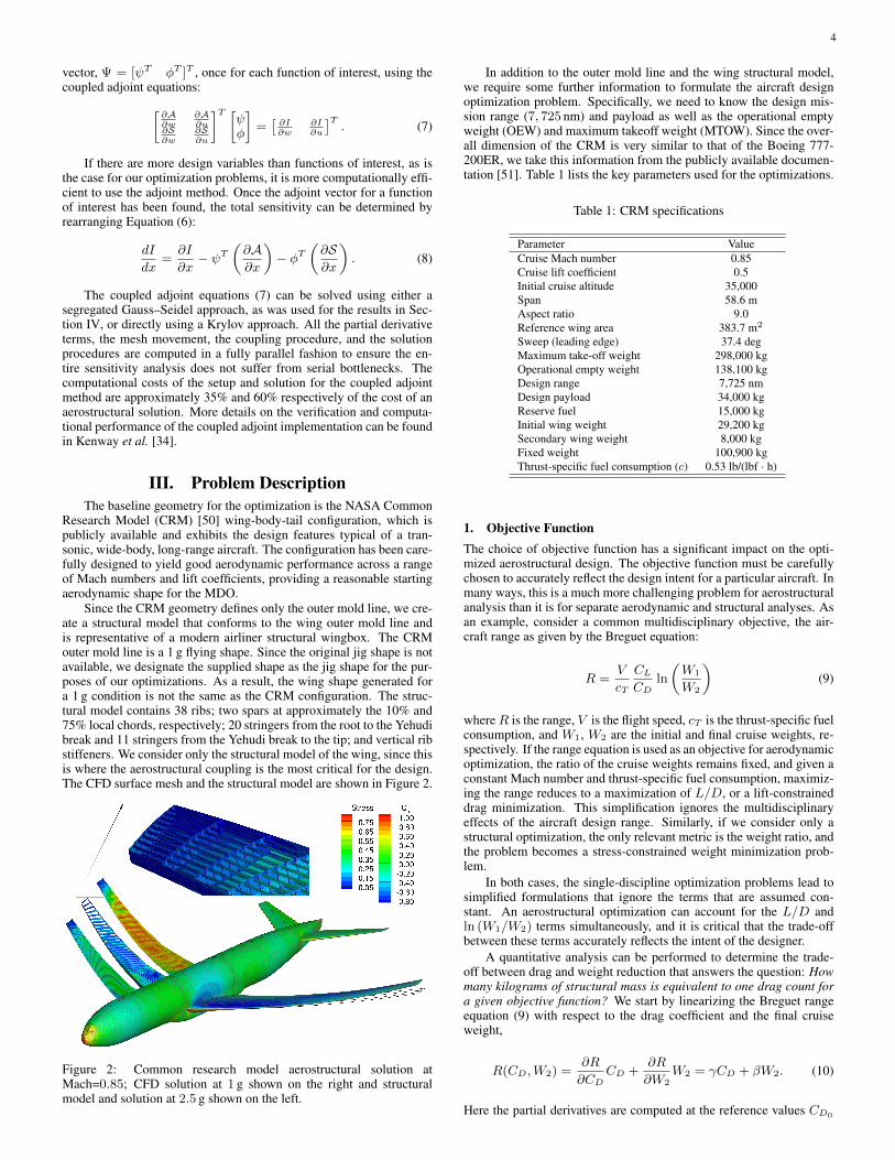
Since the CRM geometry defines only the outer mold line, we cre-ate a structural model that conforms to the wing outer mold line andis representative of a modern airliner structural wingbox. The CRMouter mold line is a 1 g flying shape. Since the original jig shape is notavailable, we designate the supplied shape as the jig shape for the pur-poses of our optimizations. As a result, the wing shape generated fora 1 g condition is not the same as the CRM configuration. The struc-tural model contains 38 ribs; two spars at approximately the 10% and75% local chords, respectively; 20 stringers from the root to the Yehudibreak and 11 stringers from the Yehudi break to the tip; and vertical ribstiffeners. We consider only the structural model of the wing, since thisis where the aerostructural coupling is the most critical for the design.The CFD surface mesh and the structural model are shown in Figure 2.

Figure 2: Common research model aerostructural solution atMach=0.85; CFD solution at 1 g shown on the right and structuralmodel and solution at 2.5 g shown on the left.

In addition to the outer mold line and the wing structural model,we require some further information to formulate the aircraft designoptimization problem. Specifically, we need to know the design mis-sion range (7, 725 nm) and payload as well as the operational emptyweight (OEW) and maximum takeoff weight (MTOW). Since the over-all dimension of the CRM is very similar to that of the Boeing 777-200ER, we take this information from the publicly available documen-tation [51]. Table 1 lists the key parameters used for the optimizations.

Table 1: CRM specifications

Parameter ValueCruise Mach number 0.85Cruise lift coefficient 0.5Initial cruise altitude 35,000Span 58.6 mAspect ratio 9.0Reference wing area 383.7 m2

Sweep (leading edge) 37.4 degMaximum take-off weight 298,000 kgOperational empty weight 138,100 kgDesign range 7,725 nmDesign payload 34,000 kgReserve fuel 15,000 kgInitial wing weight 29,200 kgSecondary wing weight 8,000 kgFixed weight 100,900 kgThrust-specific fuel consumption (c) 0.53 lb/(lbf · h)

1. Objective FunctionThe choice of objective function has a significant impact on the opti-mized aerostructural design. The objective function must be carefullychosen to accurately reflect the design intent for a particular aircraft. Inmany ways, this is a much more challenging problem for aerostructuralanalysis than it is for separate aerodynamic and structural analyses. Asan example, consider a common multidisciplinary objective, the air-craft range as given by the Breguet equation:

R =V

cT

CL

CDln

(W1

W2

)(9)

whereR is the range, V is the flight speed, cT is the thrust-specific fuelconsumption, and W1, W2 are the initial and final cruise weights, re-spectively. If the range equation is used as an objective for aerodynamicoptimization, the ratio of the cruise weights remains fixed, and given aconstant Mach number and thrust-specific fuel consumption, maximiz-ing the range reduces to a maximization of L/D, or a lift-constraineddrag minimization. This simplification ignores the multidisciplinaryeffects of the aircraft design range. Similarly, if we consider only astructural optimization, the only relevant metric is the weight ratio, andthe problem becomes a stress-constrained weight minimization prob-lem.

In both cases, the single-discipline optimization problems lead tosimplified formulations that ignore the terms that are assumed con-stant. An aerostructural optimization can account for the L/D andln (W1/W2) terms simultaneously, and it is critical that the trade-offbetween these terms accurately reflects the intent of the designer.

A quantitative analysis can be performed to determine the trade-off between drag and weight reduction that answers the question: Howmany kilograms of structural mass is equivalent to one drag count fora given objective function? We start by linearizing the Breguet rangeequation (9) with respect to the drag coefficient and the final cruiseweight,

R(CD,W2) =∂R

∂CDCD +

∂R

∂W2W2 = γCD + βW2. (10)

Here the partial derivatives are computed at the reference values CD0

5

and W20 to yield a linearization about those values:

γ =∂R

∂CD= − V

cT

CL

C2D0

ln

(W1

W20

), (11)

β =∂R

∂W2= − V

cT

CL

CD0

1

W20

(12)

The ratio of these partial derivatives is

γ

β=∂W2

∂CD=W20

CD0

ln

(W1

W20

), (13)

This ratio γ/β corresponds to the partial derivative ∂W2/∂CD , whichquantifies the decrease in the final cruise weight that would increasethe range by the same amount as a unit decrease in the drag coefficient.Thus, the ratio γ/β answers the question above: it quantifies how manyunits of structural mass are equivalent to a unit of drag. In this case,we derived this quantity for range, but we will also derive it for TOGWand fuel burn.

The partial derivative (13) shows us that the weight-drag trade-offscales with the final cruise weight, the natural logarithm of the weightratio, and that it is inversely proportional to the cruise drag coefficient.Unlike the single-discipline optimization cases, where a simple reduc-tion of drag or weight was sufficient, this multidisciplinary objective re-quires knowledge of the aerodynamic performance, CD , and the struc-tural performance, ln (W1/W2), as well as their coupling, to determinethe correct multidisciplinary trades. This places additional burden onthe analysis, since we must include all the components of the drag andweight to achieve the correct aerostructural trade-offs, even if they arenot modeled explicitly.

In this work we consider the minimization of two objectives:TOGW and fuel burn. The TOGW objective combines the manufac-turing cost (which depends on the empty weight) and the fuel burn.The fuel burn accounts for a large portion of the direct operating cost(DOC), especially for long-range commercial aircraft. The real objec-tive function for commercial aircraft is usually a compromise betweenthese two objectives.

The TOGW is assumed to be equal to the initial cruise weight,since we consider the fuel burn only during the cruise segment andignore the fuel burned during take-off, climb, and descent. Rearrangingthe Breguet equation (9) we can obtain an expression for the TOGW,given a fixed range:

TOGW = W1 = W2e

(RcTV

CDCL

). (14)

Linearizing this objective function with respect to CD and W2 aboutthe reference point (CD0 ,W20), we obtain:

γ = eRcTCD0V CL W20

(RcTV CL

)=

W1

CD0

ln

(W1

W20

), (15)

β = eRcTCD0V CL =

W1

W20

. (16)

The ratio of these two sensitivities is

γ

β=W20

CD0

ln

(W1

W20

). (17)

An equation for the cruise-segment fuel burn can also be obtainedfrom the Breguet equation (9) as follows:

Wf = W1 −W2 = W2

(e

(RcTV

CDCL

)− 1

). (18)

The partial derivatives of fuel burn with respect to CD and W2 are

γ = eRcTCD0V CL W20

(RcTV CL

)=

W1

CD0

ln

(W1

W20

), (19)

β = eRcTCD0V CL − 1 =

W1

W20

− 1. (20)

The ratio of these two sensitivities is

γ

β=

W1W20

CD0 (W1 −W20)ln

(W1

W20

). (21)

These partial derivatives and their ratios are summarized in Table 2.In addition, we calculated the values of these quantities for the CRMspecifications listed in Table 1.

The resulting γ/β for the TOGW is identical to that of the rangeobjective. Therefore, in the context of this linearization, maximizingthe range for a fixed TOGW is equivalent to minimizing the TOGWfor a fixed range. However, in their nonlinear form, these objectivesare not equivalent, since changing the range or TOGW will modify theresulting linearization.

The TOGW objective γ/β differs from the fuel burn γ/β by a fac-tor of (W1 −W2) /W1 = Wf/W1, which is the fuel fraction. Sincethe fuel fraction is always less than one, the γ/β ratio for the fuel-burnobjective is always higher than the one for the TOGW objective. Ahigher γ/β indicates that one drag count is equivalent to a larger mass.Thus, a higher γ/β value favors designs that have better aerodynamicperformance, where the weight is more readily increased to reduce thedrag. Lower γ/β values, on the other hand, favor structural weightreduction over drag reduction.

The fuel fraction for the CRM aircraft for the design payload andrange is (W1 −W2)/W1 = 0.372, so the fuel burn objective γ/β is2.69 times larger than the TOGW one. For the TOGW objective, 1drag count is worth approximately 313 kg, but for the fuel-burn objec-tive 1 drag count is equivalent to 842 kg. These values, however, arebased on linearizations, so they do not take into account that a reduc-tion inW2 further decreases the TOGW and fuel burn when the weightcalculation is recomputed. This analysis assumes a design range of7, 725 nm. Figure 3 shows the numerical value of the weight-dragtrade-off as a function of the range. The γ/β increases with respectto the range for both objectives, indicating that longer range aircraftshould place greater emphasis on the aerodynamic performance. Asthe range decreases, so does the fuel fraction, and the ratio of γ/β forthe two objectives grows without bounds as the range approaches zero.This dependence of γ/β on the range can only be captured with a mul-tidisciplinary analysis.

As discussed above, γ/β is much higher for the fuel-burn objectivethan for the TOGW objective. Therefore, minimizing the former ob-jective places a greater emphasis on decreasing drag, and the emphasisincreases with the range for both objectives, as shown in Figure 3. Wecan also observe that γ/β increases more rapidly with the range for theTOGW objective.

Range (nm)

(k

g/d

rag

ct.

)

0 2000 4000 6000 80000

200

400

600

800

1000

TOGW objective

Fuel burn objective

CRM design point

Figure 3: Variation of TOGW and fuel-burn objective sensitivities as afunction of design range.

For the optimizations presented in Section IV, we compute the finalcruise weight, W2, according to

W2 = W + Fixed Weight + Reserve Fuel Weight+A/Aref × Secondary Wing Weight (22)

whereW is the weight of the primary wing structure given based on thevolume of the structural finite element model, A is the projected wingarea, and Aref is the initial projected wing area. The last term is used toaccount for the weight of fasteners and other wing parts that scale withthe wing area. For each of the cruise conditions described in the fol-lowing section, the L/D ratio and the Breguet range equation are usedto determine the weight at the start of the cruise, W1. The L/D ratiofor each condition is computed by performing an aerostructural analy-sis at the weight corresponding to the midpoint of the mission. Finally,

6

Table 2: Linearization of the objectives and the values of the corresponding sensitivities for the CRM configuration

Objective, I γ = ∂I/∂CD kg per count β = ∂I/∂W2 kg per kg γ/β kg per count

TOGW W1CD0

ln(

W1W20

)497.0 W1

W201.59

W20CD0

ln(

W1W20

)312.6

Fuel burn W1CD0

ln(

W1W20

)497.0

W1−W20W20

0.59W1W20

CD0 (W1−W20 )ln

(W1W20

)842.4

for each of the objective functions considered, we use the average overeach cruise condition to formulate the composite objectives.

2. Design and Maneuver ConditionsWe now describe the operating conditions used in the optimizations. Toevaluate the TOGW and fuel-burn objectives, we estimate the weightat the beginning of the cruise using the Breguet range equation:

R =V

cT

CL

CDln

(W1

W2

). (23)

We assume that the aircraft is able to climb continuously as fuel is con-sumed, while maintaining the same lift-to-drag ratio and cruise Machnumber. The only aerodynamic input to this computation is the overalllift-to-drag ratio of the aircraft.

While a single analysis point is sufficient to estimate the lift-to-drag ratio, single-point optimizations (especially in the transonicregime) can produce optimal performance at a single operating pointat the cost of significant degradation in other important off-design con-ditions [52]. To address this issue, we consider multi-point aerostruc-tural optimizations that compute the average performance over multi-ple flight conditions. We consider the five cruise operating conditionslisted in Table 3 and labeled C1 through C5. These points form a crossin the Mach-altitude space centered about the operating design condi-tion for the CRM configuration (M=0.85, CL=0.5), as shown in Fig-ure 4. The cruise Mach number is varied by ±0.01 and the altitudeis varied by ±1000 ft. The change in altitude effectively varies CL torepresent typical in-service variations for a given mission. The designis particularly sensitive to the cruise Mach number because of the non-linear nature of the compressible flow, and because the optimizer canusually eliminate wave drag for a single Mach number.

32

33

34

35

36

C1C2 C3

C4

C5

M2Altitude(1000ft)

0.84 0.85 0.8619

20

21

M1

Mach

Figure 4: Visualization of cruise and maneuver conditions in Mach-altitude space

Two separate maneuver conditions—labeled M1 and M2 in Ta-ble 3—are considered: a 2.5 g symmetric pull-up maneuver and a 1.3 gacceleration due to gust. M1 represents a 2.5 g limit load for the wingstructure. M2 is meant to emulate the unsteady gust loads that in prac-tice limit the lower wing skin and stringers because of a fatigue lifelimit [53]. We implement this constraint by performing a static aeroe-lastic analysis at 1.3 g and then limiting the stress at this condition toa value that is significantly lower than the yield stress, which is deter-mined based on the fatigue life, as described in Section (III.4).

A last aerostructural analysis—labeled S1 in Table 3—is requiredto estimate the aircraft’s static margin. Using static aeroelastic analysis,

we estimate the static margin of the deformed configuration using thefollowing formula:

Kn = −CMα

CLα

. (24)

Further details on approximating static and dynamic stability deriva-tives for high-fidelity CFD optimization can be found in Mader andMartins [18]. The derivativesCMα = ∂CM/∂α andCLα = ∂CL/∂αare estimated using a forward finite-difference with step size of ∆α =0.1°. Since these coefficients are nearly linear in the range under con-sideration, we can use this relatively large finite difference step withoutsignificant truncation error, while avoiding the subtractive cancellationerrors that would show up for smaller steps. The analysis for cruisecondition 1 is used for the baseline value, and the additional stabilitypoint provides the perturbed value to complete the derivative calcula-tions.

Table 3: Operating conditions

Group Identifier Mach Altitude, ft Load factorCruise C1 0.85 35 000 1.0Cruise C2 0.84 35 000 1.0Cruise C3 0.86 35 000 1.0Cruise C4 0.85 34 000 1.0Cruise C5 0.85 36 000 1.0Maneuver M1 0.86 20 000 2.5Maneuver M2 0.85 32 000 1.3Stability S1 0.85 35 000 1.0

3. Design VariablesThe two optimizations presented use hundreds of design variables toparametrize the aerodynamic and structural models. As is typical ina multidisciplinary analysis, we can divide the design variables intoglobal variables, which directly affect more than one discipline, andlocal variables, which affect only a single discipline. Table 4 lists allthe optimization variables.

Table 4: Design variables

Description QuantityGlobal VariablesSpan 1Sweep 2Chord 4Twist 5Shape 160Aerodynamic variablesAngle of attack 1Tail rotation 1Structural variablesUpper skin 54Lower skin 54Upper stringers 54Lower stringers 54Ribs 18Rib stiffeners 18Spars 36Total 472

We use a free form deformation (FFD) volume approach to makegeometric perturbations to the geometry. Further information on our

7

Figure 5: Optimization design variables. Structural design variable grouping (left) and geometric design variables (right).

approach can be found in Kenway et al. [54]. The main wing plan-form variables, span, sweep, chord, and twist, are all global variables,since they directly affect the geometry of both the aerodynamics andthe structures. The geometric and structural design variables and theCFD mesh discretrization used for the optimization are shown in Fig-ure 5. The chords are modified at the root, Yehudi break, near tip, andtip sections, and the remaining sections are linearly interpolated. Fivetwist angles are defined similarly and interpolated linearly in the span-wise direction. Two sweep variables are specified. The first sweepsnearly the entire leading edge, which, by construction, is constrainedto remain straight. The second changes only the outer 12.5% of thewing semi-span. The shape variables are used to perturb the coeffi-cients of the FFD volume surrounding the wing in the z (normal) di-rection. These shape variables prescribe the chord and spanwise airfoilshape directly, and no additional explicit thickness or camber variablesare required. Figure 5 shows the internal layout of the structure as wellas the grouping of the structural design variables.

The structural skin-thickness variables are grouped in a grid of 18stations in the spanwise direction and 3 stations in the chordwise direc-tions, resulting in 54 variables for each of the upper and lower skins re-spectively. The stringer variables are grouped in the same way. The ribsand rib stiffeners each have 18 variables in the spanwise direction as doeach of the leading and trailing edge spars. The stringer and rib pitchesare not fixed and vary with the planform variables. Each of the fivecruise conditions and two maneuver conditions have an independentangle of attack and tail rotation angle to provide the required degreesof freedom to meet both the lift and moment constraints. Finally, themean aerodynamic chord (MAC) and center of gravity location (XCG)are target variables, each coupled with a consistency constraint thatsimplifies the implementation. This represents an interdisciplinary fea-sible MDO approach applied to these coupling variables [3]. The initialvalues for the geometric and aerodynamic design variables are chosento reproduce the original CRM geometry exactly.

To establish a reasonable initial structural design for the aerostruc-tural optimization, we optimize the wingbox by minimizing the struc-tural weight with respect to the structural thicknesses described above,subject to stress constraints for a set of fixed aerodynamic loads. Thefixed loads are obtained from aerostructural analyses at the two ma-neuver conditions described previously. The initial design consistsof a structure with linear spanwise thickness variation in each of thestructural members. The stress constraints are identical to those de-scribed in Sec. (III.4). By using design variables and constraints con-sistent with those used in the aerostructural optimizations, we provide

an initial wingbox that has already been optimized in a subspace ofthe aerostructural optimizations, and subsequent improvements in thefull space demonstrate the importance of considering both disciplines.The initial structure resulting from this optimization is shown in Fig-ures 14c and 14d.

4. Design ConstraintsIn this section we describe the constraints that are used for the TOGWand fuel-burn optimizations. For simplicity, we divide the constraintsinto three groups: geometric and target constraints, aerodynamic con-straints, and structural constraints, as shown in Table 5.

Table 5: Optimization constraints

Description QuantityGeometric/target constraintstLE/tLEInit ≥ 1.0 11tTE/tTEInit ≥ 1.0 11A/Ainit ≥ 1.0 1V /Vinit ≥ 1.0 1tTE Spar ≥ 0.20 5tTip/tTipInit

≥ 0.5 5MAC −MAC∗ = 0.0 1XCG −X∗CG = 0.0 1Aerodynamic constraintsCruise: L−W = 0.0 5Cruise: Cmy = 0.0 5Maneuver: L−W = 0.0 2Maneuver: Cmy = 0.0 2Static margin: Kn ≥ 0.15 1Structural constraints2.5g Lower skin: KS ≤ 1.0 12.5g Upper skin: KS ≤ 1.0 12.5g Rib/spars: KS ≤ 1.0 11.3g Lower skin: KS ≤ 0.42 11.3g Upper skin: KS ≤ 1.0 11.3g Rib/spars: KS ≤ 1.0 1Total 57

The first two geometric constraints, tLE and tTE, are used to con-strain the initial wing thickness at the 2.5% and 97.5% chords. Thethickness constraints at the leading edge constrain the leading-edge ra-dius and help to ensure that the high-speed aerostructural optimization

8

does not significantly impact the low speed CLmax performance, whichis largely governed by the roundness of the leading edge. The thick-ness constraints at the trailing edge prevent the upper and lower sur-faces from crossover near the sharp trailing edge. The projected wingarea is constrained to be no less than the initial area. This constraintis used to ensure adequate takeoff field length approach speed. Evenwith a complete structural model, a minimum fuel-volume constraintis required. Only the volume inside the spar-box is computed to ensurethat the optimized wing is able to carry at least the same amount of fuelas the initial design.

Several additional thickness constraints are also enforced. Min-imum trailing-edge spar height constraints, tTE spar, are used over theoutboard section of the wing. These constraints are intended to ensurethat adequate vertical space is available to attach the actuation devicesrequired for the flaps and ailerons. The tip thickness constraint, ttip, isused to ensure that the optimization does not produce an unrealisticallythin wing tip.

Each cruise and maneuver condition enforces equality constraintson the lift and pitching moment coefficient, so that all the aerostruc-tural solutions are trimmed. The static margin of the C1 condition isconstrained to be greater than 15%. The reference point for the mo-ment computation is taken to be at 25% of MAC, which changes withthe planform design variables. By including a pitch moment constraintas well as a constraint on the full configuration static margin, we allowthe optimization to trade drag reduction from aft-loaded supercriticalprofiles with the induced drag penalty required to trim the configura-tion.

Lastly, we must constrain the stresses on the structure. The struc-tural model used for the optimization consists of over 50 000 second-order MITC shell elements [55]. Individually constraining the stressin each of these elements would require the solution of the correspond-ing number of coupled adjoint vectors, which would incur a prohibitivecomputational cost. To dramatically reduce the number of solutions re-quired, we use the Kreisselmeir-Steinhauser (KS) constraint aggrega-tion technique [49, 56] that conservatively estimates the maximum of aset of stresses in a smooth and differentiabale manner. Each maneuvercondition uses three KS functions: the first for the lower wing skin andstringers, the second for the upper wing skin and stringers, and the thirdfor the spars, ribs, and rib stiffeners. The compression members in theupper wing skin and stringers are assumed to be Aluminum 7050 with amaximum allowable stress of 300 MPa. The remainder of the primarywing structure is assumed to be manufactured from Aluminum 2024with a maximum allowable stress of 324 MPa.

For the first maneuver condition, the maximum vonMises stressmust be below the limiting stress, which requires the three KS functionsto be less than 1. For the second maneuver constraint, which is relatedto fatigue, we limit the stress on the lower wing skin and stringers tobe below 138 MPa for the 1.3 g load condition, corresponding to anupper limit of 0.42 [53]. The remaining two KS functions for the 1.3 gmaneuver condition retain the maximum KS value of 1.

5. Optimization AlgorithmFor design optimization problems with hundreds of design variables(476 in our case), and objective and constraint evaluations requiring onthe order of several minutes, a gradient-based optimization algorithmis the only viable option to get an accurate answer in under two days.For this work we use SNOPT [57], an optimizer based on the SQPapproach. SNOPT is well suited for large-scale constrained nonlinearoptimization problems. The combination of the coupled adjoint, whichcan compute the gradient of a function of interest in approximatelythe same time as a function evaluation, with effective gradient-basedoptimization, enable us to solve each optimization problem in approx-imately 36 hours.

6. Computational ResourcesThe two optimizations are performed on a massively parallel super-computer [58]. Each optimization function evaluation requires the so-lution of eight aerostructural solutions: five for the cruise conditions,two for the maneuver conditions, and one for the stability point. Toreduce the wall time required for the optimizations, these parallel anal-yses are carried out concurrently. The cruise conditions and stability

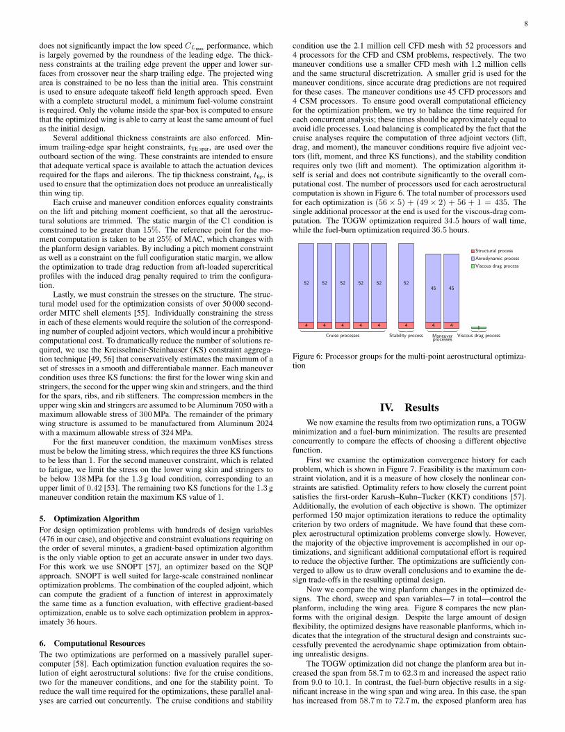
condition use the 2.1 million cell CFD mesh with 52 processors and4 processors for the CFD and CSM problems, respectively. The twomaneuver conditions use a smaller CFD mesh with 1.2 million cellsand the same structural discretrization. A smaller grid is used for themaneuver conditions, since accurate drag predictions are not requiredfor these cases. The maneuver conditions use 45 CFD processors and4 CSM processors. To ensure good overall computational efficiencyfor the optimization problem, we try to balance the time required foreach concurrent analysis; these times should be approximately equal toavoid idle processes. Load balancing is complicated by the fact that thecruise analyses require the computation of three adjoint vectors (lift,drag, and moment), the maneuver conditions require five adjoint vec-tors (lift, moment, and three KS functions), and the stability conditionrequires only two (lift and moment). The optimization algorithm it-self is serial and does not contribute significantly to the overall com-putational cost. The number of processors used for each aerostructuralcomputation is shown in Figure 6. The total number of processors usedfor each optimization is (56× 5) + (49× 2) + 56 + 1 = 435. Thesingle additional processor at the end is used for the viscous-drag com-putation. The TOGW optimization required 34.5 hours of wall time,while the fuel-burn optimization required 36.5 hours.

4

52

4

52

4

52

4

52

4

52

4

52

4

45

4

45

1

Structural process

Aerodynamic process

Viscous drag process

︸ ︷︷ ︸Cruise processes

︸ ︷︷ ︸Stability process

︸ ︷︷ ︸Maneuverprocesses

︸ ︷︷ ︸Viscous drag process

Figure 6: Processor groups for the multi-point aerostructural optimiza-tion

IV. ResultsWe now examine the results from two optimization runs, a TOGW

minimization and a fuel-burn minimization. The results are presentedconcurrently to compare the effects of choosing a different objectivefunction.

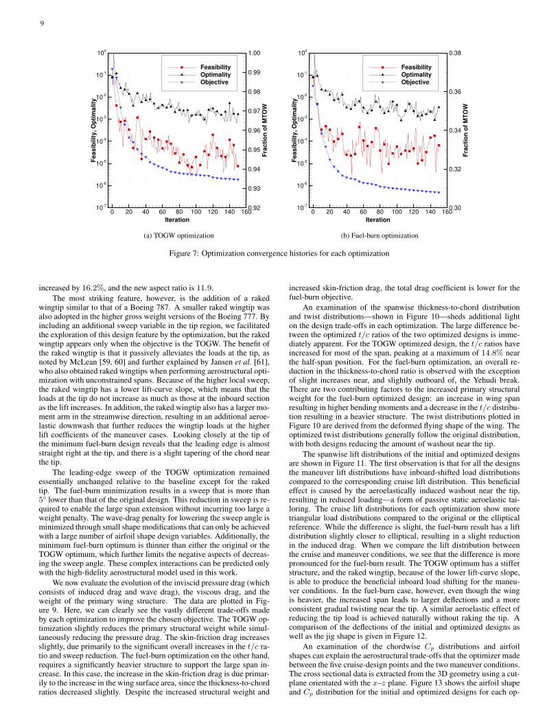
First we examine the optimization convergence history for eachproblem, which is shown in Figure 7. Feasibility is the maximum con-straint violation, and it is a measure of how closely the nonlinear con-straints are satisfied. Optimality refers to how closely the current pointsatisfies the first-order Karush–Kuhn–Tucker (KKT) conditions [57].Additionally, the evolution of each objective is shown. The optimizerperformed 150 major optimization iterations to reduce the optimalitycriterion by two orders of magnitude. We have found that these com-plex aerostructural optimization problems converge slowly. However,the majority of the objective improvement is accomplished in our op-timizations, and significant additional computational effort is requiredto reduce the objective further. The optimizations are sufficiently con-verged to allow us to draw overall conclusions and to examine the de-sign trade-offs in the resulting optimal design.

Now we compare the wing planform changes in the optimized de-signs. The chord, sweep and span variables—7 in total—control theplanform, including the wing area. Figure 8 compares the new plan-forms with the original design. Despite the large amount of designflexibility, the optimized designs have reasonable planforms, which in-dicates that the integration of the structural design and constraints suc-cessfully prevented the aerodynamic shape optimization from obtain-ing unrealistic designs.

The TOGW optimization did not change the planform area but in-creased the span from 58.7 m to 62.3 m and increased the aspect ratiofrom 9.0 to 10.1. In contrast, the fuel-burn objective results in a sig-nificant increase in the wing span and wing area. In this case, the spanhas increased from 58.7 m to 72.7 m, the exposed planform area has

9

Iteration

Fe

as

ibilit

y, O

pti

ma

lity

Fra

cti

on

of

MT

OW

0 20 40 60 80 100 120 140 16010

­7

10­6

10­5

10­4

10­3

10­2

10­1

100

0.92

0.93

0.94

0.95

0.96

0.97

0.98

0.99

1.00

Feasibility

Optimality

Objective

(a) TOGW optimization

Iteration

Fe

as

ibilit

y, O

pti

ma

lity

Fra

cti

on

of

MT

OW

0 20 40 60 80 100 120 140 16010

­7

10­6

10­5

10­4

10­3

10­2

10­1

100

0.30

0.32

0.34

0.36

0.38

Feasibility

Optimality

Objective

(b) Fuel-burn optimization

Figure 7: Optimization convergence histories for each optimization

increased by 16.2%, and the new aspect ratio is 11.9.The most striking feature, however, is the addition of a raked

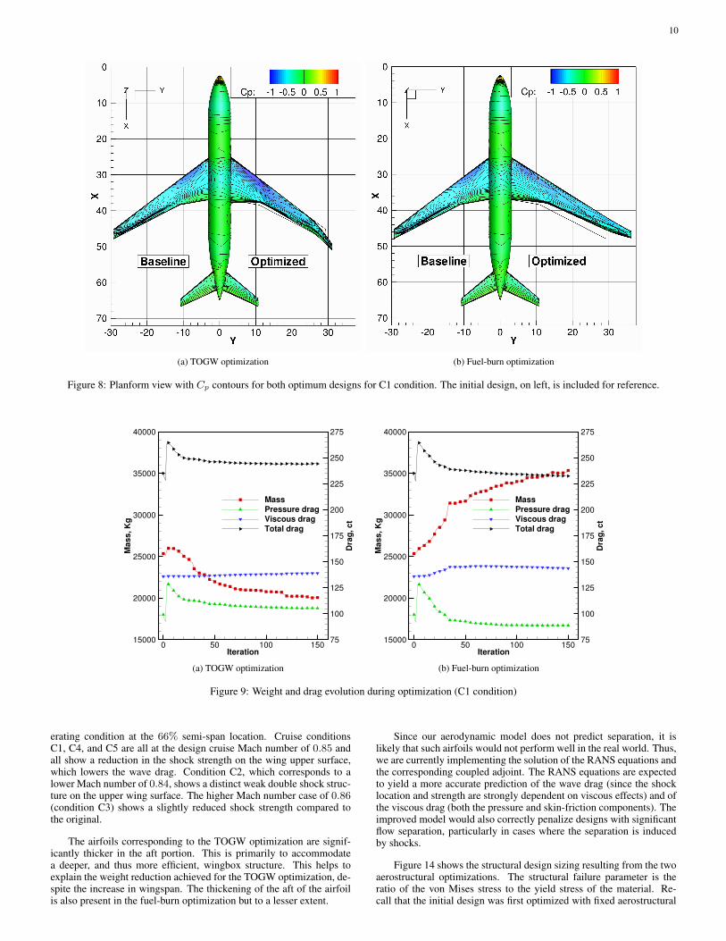
wingtip similar to that of a Boeing 787. A smaller raked wingtip wasalso adopted in the higher gross weight versions of the Boeing 777. Byincluding an additional sweep variable in the tip region, we facilitatedthe exploration of this design feature by the optimization, but the rakedwingtip appears only when the objective is the TOGW. The benefit ofthe raked wingtip is that it passively alleviates the loads at the tip, asnoted by McLean [59, 60] and further explained by Jansen et al. [61],who also obtained raked wingtips when performing aerostructural opti-mization with unconstrained spans. Because of the higher local sweep,the raked wingtip has a lower lift-curve slope, which means that theloads at the tip do not increase as much as those at the inboard sectionas the lift increases. In addition, the raked wingtip also has a larger mo-ment arm in the streamwise direction, resulting in an additional aeroe-lastic downwash that further reduces the wingtip loads at the higherlift coefficients of the maneuver cases. Looking closely at the tip ofthe minimum fuel-burn design reveals that the leading edge is almoststraight right at the tip, and there is a slight tapering of the chord nearthe tip.

The leading-edge sweep of the TOGW optimization remainedessentially unchanged relative to the baseline except for the rakedtip. The fuel-burn minimization results in a sweep that is more than5° lower than that of the original design. This reduction in sweep is re-quired to enable the large span extension without incurring too large aweight penalty. The wave-drag penalty for lowering the sweep angle isminimized through small shape modifications that can only be achievedwith a large number of airfoil shape design variables. Additionally, theminimum fuel-burn optimum is thinner than either the original or theTOGW optimum, which further limits the negative aspects of decreas-ing the sweep angle. These complex interactions can be predicted onlywith the high-fidelity aerostructural model used in this work.

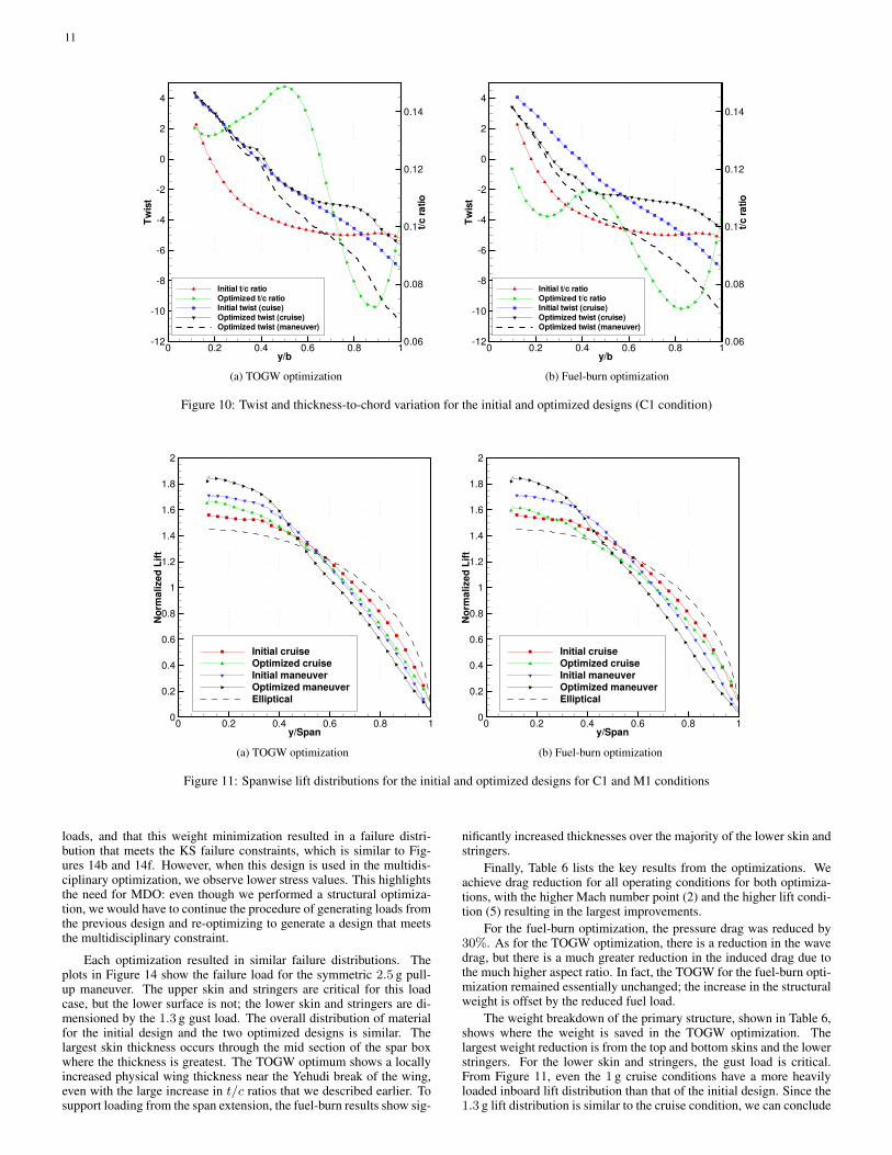
We now evaluate the evolution of the inviscid pressure drag (whichconsists of induced drag and wave drag), the viscous drag, and theweight of the primary wing structure. The data are plotted in Fig-ure 9. Here, we can clearly see the vastly different trade-offs madeby each optimization to improve the chosen objective. The TOGW op-timization slightly reduces the primary structural weight while simul-taneously reducing the pressure drag. The skin-friction drag increasesslightly, due primarily to the significant overall increases in the t/c ra-tio and sweep reduction. The fuel-burn optimization on the other hand,requires a significantly heavier structure to support the large span in-crease. In this case, the increase in the skin-friction drag is due primar-ily to the increase in the wing surface area, since the thickness-to-chordratios decreased slightly. Despite the increased structural weight and

increased skin-friction drag, the total drag coefficient is lower for thefuel-burn objective.

An examination of the spanwise thickness-to-chord distributionand twist distributions—shown in Figure 10—sheds additional lighton the design trade-offs in each optimization. The large difference be-tween the optimized t/c ratios of the two optimized designs is imme-diately apparent. For the TOGW optimized design, the t/c ratios haveincreased for most of the span, peaking at a maximum of 14.8% nearthe half-span position. For the fuel-burn optimization, an overall re-duction in the thickness-to-chord ratio is observed with the exceptionof slight increases near, and slightly outboard of, the Yehudi break.There are two contributing factors to the increased primary structuralweight for the fuel-burn optimized design: an increase in wing spanresulting in higher bending moments and a decrease in the t/c distribu-tion resulting in a heavier structure. The twist distributions plotted inFigure 10 are derived from the deformed flying shape of the wing. Theoptimized twist distributions generally follow the original distribution,with both designs reducing the amount of washout near the tip.

The spanwise lift distributions of the initial and optimized designsare shown in Figure 11. The first observation is that for all the designsthe maneuver lift distributions have inboard-shifted load distributionscompared to the corresponding cruise lift distribution. This beneficialeffect is caused by the aeroelastically induced washout near the tip,resulting in reduced loading—a form of passive static aeroelastic tai-loring. The cruise lift distributions for each optimization show moretriangular load distributions compared to the original or the ellipticalreference. While the difference is slight, the fuel-burn result has a liftdistribution slightly closer to elliptical, resulting in a slight reductionin the induced drag. When we compare the lift distribution betweenthe cruise and maneuver conditions, we see that the difference is morepronounced for the fuel-burn result. The TOGW optimum has a stifferstructure, and the raked wingtip, because of the lower lift-curve slope,is able to produce the beneficial inboard load shifting for the maneu-ver conditions. In the fuel-burn case, however, even though the wingis heavier, the increased span leads to larger deflections and a moreconsistent gradual twisting near the tip. A similar aeroelastic effect ofreducing the tip load is achieved naturally without raking the tip. Acomparison of the deflections of the initial and optimized designs aswell as the jig shape is given in Figure 12.

An examination of the chordwise Cp distributions and airfoilshapes can explain the aerostructural trade-offs that the optimizer madebetween the five cruise-design points and the two maneuver conditions.The cross sectional data is extracted from the 3D geometry using a cut-plane orientated with the x–z plane. Figure 13 shows the airfoil shapeand Cp distribution for the initial and optimized designs for each op-

10

(a) TOGW optimization (b) Fuel-burn optimization

Figure 8: Planform view with Cp contours for both optimum designs for C1 condition. The initial design, on left, is included for reference.

Iteration

Ma

ss

, K

g

Dra

g, c

t

0 50 100 15015000

20000

25000

30000

35000

40000

75

100

125

150

175

200

225

250

275

Mass

Pressure drag

Viscous drag

Total drag

(a) TOGW optimization

Iteration

Ma

ss

, K

g

Dra

g, c

t

0 50 100 15015000

20000

25000

30000

35000

40000

75

100

125

150

175

200

225

250

275

Mass

Pressure drag

Viscous drag

Total drag

(b) Fuel-burn optimization

Figure 9: Weight and drag evolution during optimization (C1 condition)

erating condition at the 66% semi-span location. Cruise conditionsC1, C4, and C5 are all at the design cruise Mach number of 0.85 andall show a reduction in the shock strength on the wing upper surface,which lowers the wave drag. Condition C2, which corresponds to alower Mach number of 0.84, shows a distinct weak double shock struc-ture on the upper wing surface. The higher Mach number case of 0.86(condition C3) shows a slightly reduced shock strength compared tothe original.

The airfoils corresponding to the TOGW optimization are signif-icantly thicker in the aft portion. This is primarily to accommodatea deeper, and thus more efficient, wingbox structure. This helps toexplain the weight reduction achieved for the TOGW optimization, de-spite the increase in wingspan. The thickening of the aft of the airfoilis also present in the fuel-burn optimization but to a lesser extent.

Since our aerodynamic model does not predict separation, it islikely that such airfoils would not perform well in the real world. Thus,we are currently implementing the solution of the RANS equations andthe corresponding coupled adjoint. The RANS equations are expectedto yield a more accurate prediction of the wave drag (since the shocklocation and strength are strongly dependent on viscous effects) and ofthe viscous drag (both the pressure and skin-friction components). Theimproved model would also correctly penalize designs with significantflow separation, particularly in cases where the separation is inducedby shocks.

Figure 14 shows the structural design sizing resulting from the twoaerostructural optimizations. The structural failure parameter is theratio of the von Mises stress to the yield stress of the material. Re-call that the initial design was first optimized with fixed aerostructural

11

y/b

Twist

t/cratio

0 0.2 0.4 0.6 0.8 1­12

­10

­8

­6

­4

­2

0

2

4

0.06

0.08

0.1

0.12

0.14

Initial t/c ratioOptimized t/c ratioInitial twist (cuise)Optimized twist (cruise)Optimized twist (maneuver)

(a) TOGW optimization

y/b

Twist

t/cratio

0 0.2 0.4 0.6 0.8 1­12

­10

­8

­6

­4

­2

0

2

4

0.06

0.08

0.1

0.12

0.14

Initial t/c ratioOptimized t/c ratioInitial twist (cruise)Optimized twist (cruise)Optimized twist (maneuver)

(b) Fuel-burn optimization

Figure 10: Twist and thickness-to-chord variation for the initial and optimized designs (C1 condition)

y/Span

No

rma

lize

d L

ift

0 0.2 0.4 0.6 0.8 10

0.2

0.4

0.6

0.8

1

1.2

1.4

1.6

1.8

2

Initial cruise

Optimized cruise

Initial maneuver

Optimized maneuver

Elliptical

(a) TOGW optimization

y/Span

No

rma

lize

d L

ift

0 0.2 0.4 0.6 0.8 10

0.2

0.4

0.6

0.8

1

1.2

1.4

1.6

1.8

2

Initial cruise

Optimized cruise

Initial maneuver

Optimized maneuver

Elliptical

(b) Fuel-burn optimization

Figure 11: Spanwise lift distributions for the initial and optimized designs for C1 and M1 conditions

loads, and that this weight minimization resulted in a failure distri-bution that meets the KS failure constraints, which is similar to Fig-ures 14b and 14f. However, when this design is used in the multidis-ciplinary optimization, we observe lower stress values. This highlightsthe need for MDO: even though we performed a structural optimiza-tion, we would have to continue the procedure of generating loads fromthe previous design and re-optimizing to generate a design that meetsthe multidisciplinary constraint.

Each optimization resulted in similar failure distributions. Theplots in Figure 14 show the failure load for the symmetric 2.5 g pull-up maneuver. The upper skin and stringers are critical for this loadcase, but the lower surface is not; the lower skin and stringers are di-mensioned by the 1.3 g gust load. The overall distribution of materialfor the initial design and the two optimized designs is similar. Thelargest skin thickness occurs through the mid section of the spar boxwhere the thickness is greatest. The TOGW optimum shows a locallyincreased physical wing thickness near the Yehudi break of the wing,even with the large increase in t/c ratios that we described earlier. Tosupport loading from the span extension, the fuel-burn results show sig-

nificantly increased thicknesses over the majority of the lower skin andstringers.

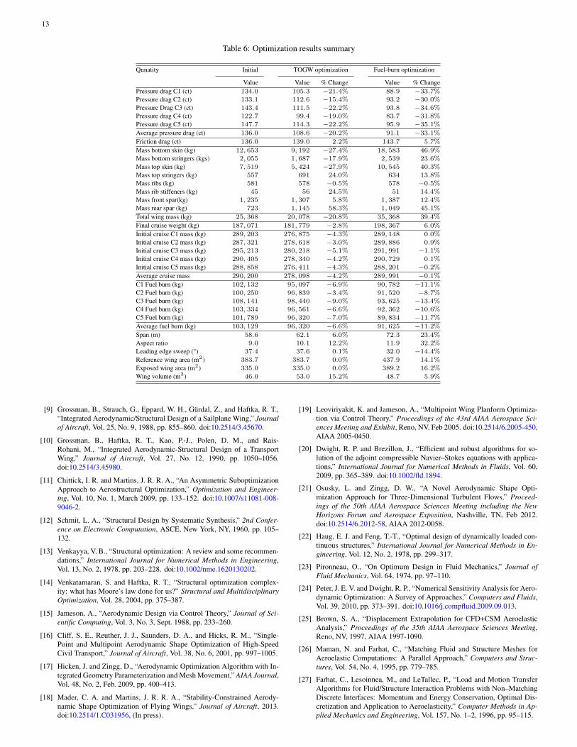
Finally, Table 6 lists the key results from the optimizations. Weachieve drag reduction for all operating conditions for both optimiza-tions, with the higher Mach number point (2) and the higher lift condi-tion (5) resulting in the largest improvements.

For the fuel-burn optimization, the pressure drag was reduced by30%. As for the TOGW optimization, there is a reduction in the wavedrag, but there is a much greater reduction in the induced drag due tothe much higher aspect ratio. In fact, the TOGW for the fuel-burn opti-mization remained essentially unchanged; the increase in the structuralweight is offset by the reduced fuel load.

The weight breakdown of the primary structure, shown in Table 6,shows where the weight is saved in the TOGW optimization. Thelargest weight reduction is from the top and bottom skins and the lowerstringers. For the lower skin and stringers, the gust load is critical.From Figure 11, even the 1 g cruise conditions have a more heavilyloaded inboard lift distribution than that of the initial design. Since the1.3 g lift distribution is similar to the cruise condition, we can conclude

12

Figure 12: Front view showing aerostructural deflections for M1 condition (left) and C1 condition (right)

that the slight induced drag penalty from a more linear lift distributionis offset by the weight reduction in the lower skin and stringers. For thefuel-burn optimization, we see weight increases across almost all of thecomponents, with the largest increases in the skins and rear spar. Giventhe reduced t/c ratio and increased span, these increases are expected.

The structural analysis in this work considered only a linear struc-tural response. The large deflections observed for the 2.5 g maneuvercondition call this assumption into question. TACS is capable of an-alyzing a geometrically nonlinear structural response, and this couldbe incorporated in the future. Since the rib and stringer pitches in-crease with increases in span and chord, respectively, we would like toinclude buckling constraints to more accurately capture the weight in-crease due to these changes. Since composite structures are playing anincreasingly important role in commercial aircraft, we would also liketo consider composite wing box structures, as done in previous workwith lower fidelity aerodynamics by Kennedy and Martins [40].

Finally, as we begin to examine more operating conditions, it be-comes increasingly important to decide how to combine the perfor-mance parameters from each analysis into a composite objective func-tion that is realistic. A weighted average can be used to assign moreimportance to certain operating conditions, but it is not straightforwardto select these weights and to measure their effect on the optimum de-sign. We are currently investigating the use of surrogate models to ap-proximate the aerostructural performance in the cruise regime to allowmore complex mission analysis and incorporate actual aircraft usagepatterns into the objective formulation [62].

V. ConclusionsIn this paper, we presented an approach for obtaining optimal static

aeroelastic tailoring of aircraft wings. We performed aerostructuraloptimizations of the NASA CRM geometry with a structure created tobe representative of a modern airliner wing. Multi-point optimizationswith 5 cruise conditions and 2 maneuver conditions were performedwith a 2 million cell CFD mesh and 300 000 DOF structural mesh. Theoptimization problems were solved with respect to 476 design variablessubject to 57 geometric, trim, and stress constraints. The solution ofthese problems required 36 hours of wall time using 435 processors.

The solution of these high-fidelity, high-dimensional design prob-lems was enabled by a scalable parallel aerostructural solver and thecombination of an efficient method for computing coupled derivativestogether with a state-of-the-art gradient-based optimizer. TOGW andfuel burn were minimized in separate design optimization problems,providing insights into the aerostructural trade-offs of transonic wingdesign.

A sensitivity analysis of each objective function showed that thefuel-burn objective should result in an optimum with lower drag thanthe TOGW objective. The optimized results show that this is indeedthe case: the fuel-burn optimization reduced the cruise-segment fuelconsumption by 11.2%, while the TOGW optimization reduced thefuel burn by 6.6%. Conversely, the TOGW minimization resulted ina 4.2% reduction in the TOGW, while the TOGW for the fuel-burnoptimization remained practically unchanged.

The minimum TOGW configuration exhibited a raked wingtip sim-ilar to that seen in the Boeing 787, which shifts the spanwise lift dis-

tribution inboard at the maneuver conditions. This is a form of passiveload alleviation that can only be found by simultaneous considerationof the aerodynamics and structures. The minimum fuel burn resultedin a wing with a span 18% larger than the TOGW one. This increase inspan came at the cost of 76% higher wing structure mass, but ultimatelyreduced the fuel burn relative to the TOGW case by 4.9%.

The optimization results demonstrate that the proposed approachperforms trade-offs between aerodynamic and structural performancein an effective way, taking into account the chosen objective. Weare now capable of performing the aerostructural design optimizationof full configurations with respect to hundreds of aerodynamic shapeand structural sizing design variables, subject to real-world constraints.This is a promising approach for designing the wings of future air-craft, which are expected exhibit large span wings that are more flexi-ble. This trend in larger span wings is likely to continue as the price offuel increases (shifting the trade-off to higher mass, lower induced dragwings), and as better materials and structural designs emerge (enablinglarger span for a given structural mass). This shift in the aerostructuraltrade-offs will change the design space, and the approach proposed inthis paper provides an effective tool to explore this new design space,while taking full advantage of static aeroelastic tailoring.

VI. AcknowledgmentsThe authors are grateful for the funding provided by the Natural

Sciences and Engineering Research Council. The computations wereperformed on the GPC (General Purpose Cluster) supercomputer at theSciNet HPC Consortium. SciNet is funded by the Canada Foundationfor Innovation under the auspices of Compute Canada; the Governmentof Ontario; the Ontario Research Fund — Research Excellence; and theUniversity of Toronto.

References[1] Ashley, H., “On Making Things the Best — Aeronautical Uses of Opti-

mization,” Journal of Aircraft, Vol. 19, No. 1, Jan. 1982, pp. 5–28.

[2] Sobieszczanski-Sobieski, J. and Haftka, R. T., “MultidisciplinaryAerospace Design Optimization: Survey of Recent Developments,” Struc-tural Optimization, Vol. 14, No. 1, 1997, pp. 1–23. doi:10.1007/BF011.

[3] Martins, J. R. R. A. and Lambe, A. B., “Multidisciplinary De-sign Optimization: A Survey of Architectures,” AIAA Journal, 2013.doi:10.2514/1.J051895, (In press).

[4] Pai, S. I. and Sears, W. R., “Some Aeroelastic Properties of Swept Wings,”Journal of the Aeronautical Sciences, Vol. 16, No. 2, 1949, pp. 105–115.

[5] Brown, H., “A Method for the Determination of the Spanwise Load Dis-tribution of a Flexible Swept Wing at Subsonic Speeds,” Tech. rep., 1951,DTIC Document.

[6] Diederich, F. W., “The Calculation of the Aerodynamic Loading of Flex-ible Wings of Arbitrary Planform and Stiffness,” Tech. rep., 1949, RACTN 1876.

[7] Livne, E., “Future of Airplane Aeroelasticity,” Journal of Aircraft, Vol. 40,No. 6, 2003, pp. 1066–1092.

[8] Haftka, R. T., “Optimization of Flexible Wing Structures Subject toStrength and Induced Drag Constraints,” AIAA Journal, Vol. 14, No. 8,1977, pp. 1106–1977. doi:10.2514/3.7400.

13

Table 6: Optimization results summary

Qunatity Initial TOGW optimization Fuel-burn optimization

Value Value % Change Value % ChangePressure drag C1 (ct) 134.0 105.3 −21.4% 88.9 −33.7%

Pressure drag C2 (ct) 133.1 112.6 −15.4% 93.2 −30.0%

Pressure Drag C3 (ct) 143.4 111.5 −22.2% 93.8 −34.6%

Pressure drag C4 (ct) 122.7 99.4 −19.0% 83.7 −31.8%

Pressure drag C5 (ct) 147.7 114.3 −22.2% 95.9 −35.1%

Average pressure drag (ct) 136.0 108.6 −20.2% 91.1 −33.1%

Friction drag (ct) 136.0 139.0 2.2% 143.7 5.7%

Mass bottom skin (kg) 12, 653 9, 192 −27.4% 18, 583 46.9%

Mass bottom stringers (kgs) 2, 055 1, 687 −17.9% 2, 539 23.6%

Mass top skin (kg) 7, 519 5, 424 −27.9% 10, 545 40.3%

Mass top stringers (kg) 557 691 24.0% 634 13.8%

Mass ribs (kg) 581 578 −0.5% 578 −0.5%

Mass rib stiffeners (kg) 45 56 24.5% 51 14.4%

Mass front spar(kg) 1, 235 1, 307 5.8% 1, 387 12.4%

Mass rear spar (kg) 723 1, 145 58.3% 1, 049 45.1%

Total wing mass (kg) 25, 368 20, 078 −20.8% 35, 368 39.4%

Final cruise weight (kg) 187, 071 181, 779 −2.8% 198, 367 6.0%

Initial cruise C1 mass (kg) 289, 203 276, 875 −4.3% 289, 148 0.0%

Initial cruise C2 mass (kg) 287, 321 278, 618 −3.0% 289, 886 0.9%

Initial cruise C3 mass (kg) 295, 213 280, 218 −5.1% 291, 991 −1.1%

Initial cruise C4 mass (kg) 290, 405 278, 340 −4.2% 290, 729 0.1%

Initial cruise C5 mass (kg) 288, 858 276, 411 −4.3% 288, 201 −0.2%

Average cruise mass 290, 200 278, 098 −4.2% 289, 991 −0.1%

C1 Fuel burn (kg) 102, 132 95, 097 −6.9% 90, 782 −11.1%

C2 Fuel burn (kg) 100, 250 96, 839 −3.4% 91, 520 −8.7%

C3 Fuel burn (kg) 108, 141 98, 440 −9.0% 93, 625 −13.4%

C4 Fuel burn (kg) 103, 334 96, 561 −6.6% 92, 362 −10.6%

C5 Fuel burn (kg) 101, 789 96, 320 −7.0% 89, 834 −11.7%

Average fuel burn (kg) 103, 129 96, 320 −6.6% 91, 625 −11.2%

Span (m) 58.6 62.1 6.0% 72.3 23.4%

Aspect ratio 9.0 10.1 12.2% 11.9 32.2%

Leading edge sweep (°) 37.4 37.6 0.1% 32.0 −14.4%

Reference wing area (m2) 383.7 383.7 0.0% 437.9 14.1%

Exposed wing area (m2) 335.0 335.0 0.0% 389.2 16.2%

Wing volume (m3) 46.0 53.0 15.2% 48.7 5.9%

[9] Grossman, B., Strauch, G., Eppard, W. H., Gurdal, Z., and Haftka, R. T.,“Integrated Aerodynamic/Structural Design of a Sailplane Wing,” Journalof Aircraft, Vol. 25, No. 9, 1988, pp. 855–860. doi:10.2514/3.45670.

[10] Grossman, B., Haftka, R. T., Kao, P.-J., Polen, D. M., and Rais-Rohani, M., “Integrated Aerodynamic-Structural Design of a TransportWing,” Journal of Aircraft, Vol. 27, No. 12, 1990, pp. 1050–1056.doi:10.2514/3.45980.

[11] Chittick, I. R. and Martins, J. R. R. A., “An Asymmetric SuboptimizationApproach to Aerostructural Optimization,” Optimization and Engineer-ing, Vol. 10, No. 1, March 2009, pp. 133–152. doi:10.1007/s11081-008-9046-2.

[12] Schmit, L. A., “Structural Design by Systematic Synthesis,” 2nd Confer-ence on Electronic Computation, ASCE, New York, NY, 1960, pp. 105–132.

[13] Venkayya, V. B., “Structural optimization: A review and some recommen-dations,” International Journal for Numerical Methods in Engineering,Vol. 13, No. 2, 1978, pp. 203–228. doi:10.1002/nme.1620130202.

[14] Venkatamaran, S. and Haftka, R. T., “Structural optimization complex-ity: what has Moore’s law done for us?” Structural and MultidisciplinaryOptimization, Vol. 28, 2004, pp. 375–387.

[15] Jameson, A., “Aerodynamic Design via Control Theory,” Journal of Sci-entific Computing, Vol. 3, No. 3, Sept. 1988, pp. 233–260.

[16] Cliff, S. E., Reuther, J. J., Saunders, D. A., and Hicks, R. M., “Single-Point and Multipoint Aerodynamic Shape Optimization of High-SpeedCivil Transport,” Journal of Aircraft, Vol. 38, No. 6, 2001, pp. 997–1005.

[17] Hicken, J. and Zingg, D., “Aerodynamic Optimization Algorithm with In-tegrated Geometry Parameterization and Mesh Movement,” AIAA Journal,Vol. 48, No. 2, Feb. 2009, pp. 400–413.

[18] Mader, C. A. and Martins, J. R. R. A., “Stability-Constrained Aerody-namic Shape Optimization of Flying Wings,” Journal of Aircraft, 2013.doi:10.2514/1.C031956, (In press).

[19] Leoviriyakit, K. and Jameson, A., “Multipoint Wing Planform Optimiza-tion via Control Theory,” Proceedings of the 43rd AIAA Aerospace Sci-ences Meeting and Exhibit, Reno, NV, Feb 2005. doi:10.2514/6.2005-450,AIAA 2005-0450.

[20] Dwight, R. P. and Brezillon, J., “Efficient and robust algorithms for so-lution of the adjoint compressible Navier–Stokes equations with applica-tions,” International Journal for Numerical Methods in Fluids, Vol. 60,2009, pp. 365–389. doi:10.1002/fld.1894.

[21] Osusky, L. and Zingg, D. W., “A Novel Aerodynamic Shape Opti-mization Approach for Three-Dimensional Turbulent Flows,” Proceed-ings of the 50th AIAA Aerospace Sciences Meeting including the NewHorizons Forum and Aerospace Exposition, Nashville, TN, Feb 2012.doi:10.2514/6.2012-58, AIAA 2012-0058.

[22] Haug, E. J. and Feng, T.-T., “Optimal design of dynamically loaded con-tinuous structures,” International Journal for Numerical Methods in En-gineering, Vol. 12, No. 2, 1978, pp. 299–317.

[23] Pironneau, O., “On Optimum Design in Fluid Mechanics,” Journal ofFluid Mechanics, Vol. 64, 1974, pp. 97–110.

[24] Peter, J. E. V. and Dwight, R. P., “Numerical Sensitivity Analysis for Aero-dynamic Optimization: A Survey of Approaches,” Computers and Fluids,Vol. 39, 2010, pp. 373–391. doi:10.1016/j.compfluid.2009.09.013.

[25] Brown, S. A., “Displacement Extrapolation for CFD+CSM AeroelasticAnalysis,” Proceedings of the 35th AIAA Aerospace Sciences Meeting,Reno, NV, 1997, AIAA 1997-1090.

[26] Maman, N. and Farhat, C., “Matching Fluid and Structure Meshes forAeroelastic Computations: A Parallel Approach,” Computers and Struc-tures, Vol. 54, No. 4, 1995, pp. 779–785.

[27] Farhat, C., Lesoinnea, M., and LeTallec, P., “Load and Motion TransferAlgorithms for Fluid/Structure Interaction Problems with Non–MatchingDiscrete Interfaces: Momentum and Energy Conservation, Optimal Dis-cretization and Application to Aeroelasticity,” Computer Methods in Ap-plied Mechanics and Engineering, Vol. 157, No. 1–2, 1996, pp. 95–115.

14

[28] Kamakoti, R. and Shyy, W., “Fluid–Structure Interaction for AeroelasticApplications,” Progress in Aerospace Sciences, Vol. 40, 2004, pp. 535–558.

[29] Felippa, C. A., Park, K., and Farhat, C., “Partitioned Analysis of Cou-pled Mechanical Systems,” Computer Methods in Applied Mechanics andEngineering, Vol. 190, 2001, pp. 3247–3270.

[30] Kim, J. Y., Aluru, N. R., and Tortorelli, D. A., “Improved Multi-LevelNewton Solvers for Fully Coupled Multi-Physics Problems,” InternationalJournal for Numerical Methods in Engineering, Vol. 58, 2003, pp. 463–480. doi:10.1002/nme.751.

[31] Martins, J. R. R. A., Alonso, J. J., and Reuther, J. J., “Aero-StructuralWing Design Optimization Using High-Fidelity Sensitivity Analysis,”Proceedings of the CEAS Conference on Multidisciplinary Aircraft De-sign and Optimization, edited by H. Holinger, Koln, Germany, June 2001,pp. 211–226.

[32] Martins, J. R. R. A., Alonso, J. J., and Reuther, J. J., “A Coupled-AdjointSensitivity Analysis Method for High-Fidelity Aero-Structural Design,”Optimization and Engineering, Vol. 6, No. 1, March 2005, pp. 33–62.doi:10.1023/B:OPTE.0000048536.47956.62.

[33] Martins, J. R. R. A., Alonso, J. J., and Reuther, J. J., “High-FidelityAerostructural Design Optimization of a Supersonic Business Jet,” Jour-nal of Aircraft, Vol. 41, No. 3, 2004, pp. 523–530. doi:10.2514/1.11478.

[34] Kenway, G. K. W., Kennedy, G. J., and Martins, J. R. R. A., “A Scal-able Parallel Approach for High-Fidelity Steady-State Aeroelastic Analy-sis and Derivative Computations,” AIAA Journal, 2013, (In press).

[35] Martins, J. R. R. A. and Hwang, J. T., “Review and Unification of DiscreteMethods for Computing Derivatives of Single- and Multi-disciplinaryComputational Models,” AIAA Journal, 2013. doi:10.2514/1.J052184, (Inpress).

[36] Maute, K., Nikbay, M., and Farhat, C., “Sensitivity Analysis and DesignOptimization of Three-Dimensional Non-Linear Aeroelastic Systems bythe Adjoint Method,” International Journal for Numerical Methods in En-gineering, Vol. 56, No. 6, 2003, pp. 911–933.

[37] Barcelos, M., Bavestrello, H., and Maute, K., “A Schur-Newton-Krylov Solver for Steady-State Aeroelastic Analysis and DesignSensitivity Analysis,” Computer Methods in Applied Mechanicsand Engineering, Vol. 195, No. 17-18, 2006, pp. 2050–2069.doi:10.1016/j.cma.2004.09.013.

[38] Brezellion, J., Ronzheimer, A., Haar, D., Abu-Zurayk, M., Lummer, K.,Kruger, W., and Nattere, F. J., “Development and Application of Multi-Disciplinary Optimization Capabilities Based on High-Fidelity Methods,”53rd AIAA/ASME/ASCE/AHS/ASC Structures, Structural Dynamics, andMaterials Conference, Honolulu, HI, April 2012, AIAA 2012–1757.

[39] Ghazlane, I., Carrier, G., Dumont, A., and Desideri, J.-A.,“Aerostructural adjoint method for flexible wing optimization,” 53rdAIAA/ASME/ASCE/AHS/ASC Structures, Structural Dynamics, and Ma-terials Conference, Honolulu, HI, April 2012, AIAA 2012-1924.

[40] Kennedy, G. J. and Martins, J. R. R. A., “A Comparison of Metallic andComposite Aircraft Wings Using Aerostructural Design Optimization,”14th AIAA/ISSMO Multidisciplinary Analysis and Optimization Confer-ence, Indianapolis, IN, Sep. 2012, AIAA-2012-5475.

[41] Kennedy, G. J. and Martins, J. R. R. A., “A Laminate Parametriza-tion Technique for Discrete Ply Angle Problems with Manufactur-ing Constraints,” Structural and Multidisciplinary Optimization, 2013.doi:10.1007/s00158-013-0906-9, (In press).

[42] Piperni, P., Abdo, M., Kafyeke, F., and Isikveren, A. T., “PreliminaryAerostructural Optimization of a Large Business Jet,” Journal of Aircraft,Vol. 44, No. 5, 2007, pp. 1422–1438.

[43] DeBlois, A. and Abdo, M., “Multi-Fidelity Multidisciplinary Design Op-timization of Metallic and Composite Regional and Business Jets,” Pro-ceedings of the 13th AIAA/ISSMO Multidisciplinary Analysis and Opti-mization Conference, 2011, AIAA 2010-9191.

[44] van der Weide, E., Kalitzin, G., Schluter, J., and Alonso, J. J., “UnsteadyTurbomachinery Computations Using Massively Parallel Platforms,” Pro-ceedings of the 44th AIAA Aerospace Sciences Meeting and Exhibit,Reno, NV, 2006, AIAA 2006–0421.

[45] Kennedy, G. J. and Martins, J. R. R. A., “Parallel Solution Methods forAerostructural Analysis and Design Optimization,” Proceedings of the13th AIAA/ISSMO Multidisciplinary Analysis and Optimization Confer-ence, Fort Worth, Texas, September 2010.

[46] Hopkins, E. J., “Charts for predicting turbulent skin friction form the VanDriest Method (II),” TN D-6945, NASA Ames Research Center, 1972.

[47] Mason, W., Program FRICTION Manual, Virginia Tech, Blacks-burg, VA, http://www.dept.aoe.vt.edu/˜mason/Mason_f/MRsoft.html.

[48] Torenbeek, E., Synthesis of Subsonic Airplane Design, Delft UniversityPress and Kluwer Academic Publishers, 6th ed., 1990.

[49] Wrenn, G., “An Indirect Method for Numerical Optimization Using theKreisselmeier-Steinhauser Function,” NASA Technical Report CR-4220,NASA, 1989.

[50] Vassberg, J. C., DeHaan, M. A., Rivers, S. M., and Wahls, R. A., “De-velopment of a Common Research Model for Applied CFD ValidationStudies,” 26th AIAA Applied Aerodynamics Conference, AIAA, Honolulu,Hawaii, August 2008.

[51] Boeing Commercial Airplanes, “777-200/300 Airplane Characteristics forAirport Planning,” Internet, July 1998, D6-58329.

[52] Nemec, M., Zingg, D. W., and Pulliam, T. H., “Multipoint and Multi-Objective Aerodynamic Shape Optimization,” AIAA Journal, Vol. 42,No. 6, June 2004, pp. 1057–1065.

[53] Hurlimann, F., Mass Estimation of Transport Aircraft Wing, Ph.D. thesis,ETH Zurich, 2010.

[54] Kenway, G. K. W., Kennedy, G. J., and Martins, J. R. R. A., “ACAD-Free Approach to High-Fidelity Aerostructural Optimization,” 13thAIAA/ISSMO Multidisciplinary Analysis and Optimization Conference,Fort Worth, TX, September 2010, AIAA–2010–9231.

[55] Dvorkin, E. N. and Bathe, K.-J., “A Continuum Mechanics Based Four-Node Shell Element for General Nonlinear Analysis,” Engineering Com-putations, Vol. 1, No. 1, 1984, pp. 77–88.

[56] Poon, N. M. K. and Martins, J. R. R. A., “An Adaptive Approach toConstraint Aggregation Using Adjoint Sensitivity Analysis,” Structuresand Multidisciplinary Optimization, Vol. 30, No. 1, 2007, pp. 61–73.doi:10.1007/s00158-006-0061-7.

[57] Gill, P. E., Murray, W., and Saunders, M. A., “SNOPT: An SQP Algorithmfor Large-Scale Constrained Optimization,” SIAM Review, Vol. 47, No. 1,2005, pp. 99–131. doi:10.1137/S0036144504446096.

[58] Loken, C., Gruner, D., Groer, L., Peltier, R., Bunn, N., Craig, M., Hen-riques, T., Dempsey, J., Yu, C.-H., Chen, J., Dursi, L. J., Chong, J.,Northrup, S., Pinto, J., Knecht, N., and Zon, R. V., “SciNet: LessonsLearned from Building a Power-Efficient Top-20 System and Data Cen-tre,” Journal of Physics: Conference Series, Vol. 256, No. 1, 2010,pp. 012026.

[59] McLean, D., “Wingtip Devices: What They Do and How They Do It,”Proceedings of the Boeing Performance and Flight Operations Engineer-ing Conference, 2005.

[60] McLean, D., Understanding Aerodynamics: arguing from the real physics,Wiley, 2013.

[61] Jansen, P., Perez, R. E., and Martins, J. R. R. A., “Aerostructural Op-timization of Nonplanar Lifting Surfaces,” Journal of Aircraft, Vol. 47,No. 5, 2010, pp. 1491–1503. doi:10.2514/1.44727.

[62] Liem, R. P., Kenway, G. K., and Martins, J. R. R. A., “Multi-point, multi-mission, high-fidelity aerostructural optimization of a long-range aircraftconfiguration,” Proceedings of the 14th AIAA/ISSMO MultidisciplinaryAnalysis and Optimization Conference, Indianapolis, IN, Sept. 2012.

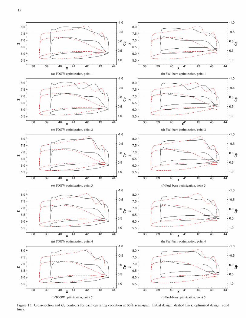
15

X

Z Cp

38 39 40 41 42 43 44

5.5

6.0

6.5

7.0

7.5

8.0

­1.0

­0.5

0.0

0.5

1.0

(a) TOGW optimization, point 1

X

Z Cp

38 39 40 41 42 43 44

5.5

6.0

6.5

7.0

7.5

8.0

­1.0

­0.5

0.0

0.5

1.0

(b) Fuel-burn optimization, point 1

X

Z Cp

38 39 40 41 42 43 44

5.5

6.0

6.5

7.0

7.5

8.0

­1.0

­0.5

0.0

0.5

1.0

(c) TOGW optimization, point 2

X

Z Cp

38 39 40 41 42 43 44

5.5

6.0

6.5

7.0

7.5

8.0

­1.0

­0.5

0.0

0.5

1.0

(d) Fuel-burn optimization, point 2

X

Z Cp

38 39 40 41 42 43 44

5.5

6.0

6.5

7.0

7.5

8.0

­1.0

­0.5

0.0

0.5

1.0

(e) TOGW optimization, point 3

X

Z Cp

38 39 40 41 42 43 44

5.5

6.0

6.5

7.0

7.5

8.0

­1.0

­0.5

0.0

0.5

1.0

(f) Fuel-burn optimization, point 3

X

Z Cp

38 39 40 41 42 43 44

5.5

6.0

6.5

7.0

7.5

8.0

­1.0

­0.5

0.0

0.5

1.0

(g) TOGW optimization, point 4

X

Z Cp

38 39 40 41 42 43 44

5.5

6.0

6.5

7.0

7.5

8.0

­1.0

­0.5

0.0

0.5

1.0

(h) Fuel-burn optimization, point 4

X

Z Cp

38 39 40 41 42 43 44

5.5

6.0

6.5

7.0

7.5

8.0

­1.0

­0.5

0.0

0.5

1.0

(i) TOGW optimization, point 5

X

Z Cp

38 39 40 41 42 43 44

5.5

6.0

6.5

7.0

7.5

8.0

­1.0

­0.5

0.0

0.5

1.0

(j) Fuel-burn optimization, point 5

Figure 13: Cross-section and Cp contours for each operating condition at 66% semi-span. Initial design: dashed lines; optimized design: solidlines.

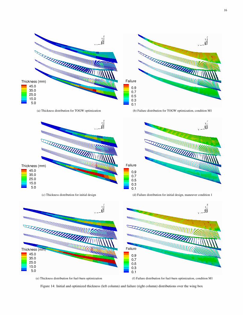
16

(a) Thickness distribution for TOGW optimization (b) Failure distribution for TOGW optimization, condition M1

(c) Thickness distribution for initial design (d) Failure distribution for initial design, maneuver condition 1

(e) Thickness distribution for fuel-burn optimization (f) Failure distribution for fuel-burn optimization, condition M1

Figure 14: Initial and optimized thickness (left column) and failure (right column) distributions over the wing box