A multi-asset investment and consumption problem with

Finance Stoch (2019) 23:641–676https://doi.org/10.1007/s00780-019-00391-6

A multi-asset investment and consumption problemwith transaction costs

David Hobson1 · Alex S.L. Tse2 · Yeqi Zhu3

Received: 10 November 2016 / Accepted: 5 March 2019 / Published online: 28 May 2019© The Author(s) 2019

Abstract In this article, we study a multi-asset version of the Merton investmentand consumption problem with CRRA utility and proportional transaction costs. Wespecialise to a case where transaction costs are zero except for sales and purchasesof a single asset which we call the illiquid asset. We show that the underlying HJBequation can be transformed into a boundary value problem for a first order differ-ential equation. Important properties of the multi-asset problem (including when theproblem is well-posed, ill-posed, or well-posed for some values of transaction costsonly) can be inferred from the behaviours of a quadratic function of a single variableand another algebraic function.

Keywords Portfolio choice · Transaction costs · Multiple assets ·Hamilton–Jacobi–Bellman equation · Free boundary value problem

Mathematics Subject Classification (2010) 91G10 · 93E20

JEL Classification G11

The opinions expressed in the paper are those of the author and not of Credit Suisse.

B D. [email protected]

A.S.L. [email protected]

Y. [email protected]

1 Department of Statistics, University of Warwick, Coventry, CV4 7AL, UK

2 Department of Mathematics, Imperial College London, London, SW7 2AZ, UK

3 Credit Suisse, London, UK

http://crossmark.crossref.org/dialog/?doi=10.1007/s00780-019-00391-6&domain=pdf

mailto:[email protected]



642 D. Hobson et al.

1 Introduction

In one of his seminal works, Merton [20] studies an optimal investment/consumptionproblem faced by a risk-averse agent over an infinite horizon. In an economy in whichthe single risky asset follows an exponential Brownian motion and the agent hasconstant relative risk aversion, the optimal strategy is to consume at a rate which isproportional to wealth, and to invest a constant fraction of wealth in the risky asset.The result generalises easily to multiple risky assets.

Constantinides and Magill [19] were the first to incorporate proportional transac-tion costs into the Merton model. They conjectured that the agent should trade mini-mally to keep the fraction of wealth invested in the risky asset within an interval. Sub-sequently, Davis and Norman [9] gave a precise characterisation of the trading strat-egy in terms of local times and formally proved its optimality by a Hamilton–Jacobi–Bellman (HJB) equation verification argument. Shreve and Soner [23] reproved theresults of [9] using viscosity solutions and gave several extensions. These approachesremain the main methods for solving portfolio optimisation problems with transac-tion costs, although recently a different technique based on shadow prices has beenproposed; see Guasoni and Muhle-Karbe [12] for a user’s guide. Kallsen and Muhle-Karbe [17], Choi et al. [6] and Herczegh and Prokaj [13] use the dual approach tocharacterise the solution to the problem with transaction costs and one risky asset.

The results in Davis and Norman [9] are limited to a single risky asset, and it isof great interest to understand how they generalise to multiple risky assets where therelated literature is limited. On the computational side in a multi-asset setting, Muthu-raman and Kumar [21] use a process of policy improvement to construct a numericalsolution for the value function and the associated no-transaction region, Collings andHaussmann [7] derive a numerical solution via a Markov chain approximation forwhich they prove convergence, and Dai and Zhong [8] use a penalty method to ob-tain numerical solutions. On the theoretical front, Akian et al. [1] show that the valuefunction is the unique viscosity solution of the HJB equation (and provide some nu-merical results in the two-asset case), and Chen and Dai [4] identify the shape of theno-transaction region in the two-asset case. Explicit solutions of the general problemremain very rare.

One situation when an explicit solution is possible is the rather special case ofuncorrelated risky assets and an agent with constant absolute risk aversion. In thatcase, the problem decouples into a family of optimisation problems, one for eachrisky asset; see Liu [18]. Another setting for which some progress has been madeis the problem with small transaction costs; see Whalley and Wilmott [26], Janecekand Shreve [16], Bichuch and Shreve [3], Soner and Touzi [24], and, for a recentanalysis in the multi-asset case, Possamaï et al. [22]. These papers use an expansionmethod to provide asymptotic formulae for the optimal strategy, value function andno-transaction region.

Our focus is on optimal investment/consumption problems, but there is a parallelliterature on optimal investment problems involving maximising expected utility ata distant terminal horizon; see for example Dumas and Luciano [10] for an explicitsolution in the one-asset case, and Bichuch and Guasoni [2] for recent work in asetting similar to ours with liquid and illiquid assets.

A multi-asset investment and consumption problem with transaction costs 643

In this paper, we consider the problem with a risk-free bond and two risky assets.1

Transactions in the first risky asset (which we call the liquid risky asset) are costless,but transactions in the second risky asset, which we term the illiquid asset, incurproportional costs. This is also the setting of a recent paper by Choi [5]. The maindifference between this paper and Choi [5] is that we analyse the HJB equation,whereas Choi takes the dual approach and studies shadow prices.

This paper is an extension of Hobson et al. [14] which considers a similar prob-lem with a bond and an illiquid asset, but with no other risky assets.2 Many of thetechniques of [14] carry over to the wider setting of the present paper. (Similarly, thepaper of Choi [5] extends the work of Choi et al. [6] to include a risky liquid asset.)However, since there are fewer parameters when the financial market includes justone risky asset, the problem in [14] is significantly simpler and much more amenableto a comparative statics analysis. In contrast, the present paper treats the multi-assetproblem which has proved so difficult to analyse, albeit in a rather special case. Themulti-asset setting brings new challenges and complicates the analysis.

Our first achievement is to show that the problem of finding the free boundariesand the value function can be reduced to the study of a family of solutions to a bound-ary crossing problem for a first order ordinary differential equation parameterised byits initial value; see Problem 3.2 below. Moreover, the existence or otherwise of a so-lution to this boundary crossing problem can be reduced to a study of the propertiesof a quadratic function and a second algebraic function. Given the results of Hobsonet al. [14] or Choi et al. [6], this is perhaps not a surprise. Nonetheless, the reductionof the problem to a first order equation is key to all subsequent developments.

Our second main achievement is to give necessary and sufficient conditions on theparameters for the problem to be well-posed (Theorem 4.1), and in those cases togive an expression for the value function (Theorem 4.3). These results extend Choiet al. [6] and Hobson et al. [14] to the case of multiple risky assets. We find that theproblem may be well-posed, or it may be ill-posed, or (if R < 1) it may be well-posedfor large transaction costs and ill-posed for small transaction costs, or (if R > 1) itmay be well-posed for small transaction costs and ill-posed for large transaction costs.

Our third achievement is to make definitive statements about the comparative stat-ics for the problem. We focus on the boundaries of the no-transaction wedge and thecertainty equivalent value of the holdings in the illiquid asset. Among other results,we prove (see Theorem 6.2 and Corollary 6.3 for precise statements) that as the re-turn on the illiquid asset improves, the agent aims to keep a larger fraction of his totalwealth in the illiquid asset, in the sense that the critical ratios at which sales and pur-chases take place are increasing in the return. Conversely, as the agent becomes moreimpatient, the agent keeps a smaller fraction of wealth in the illiquid asset. Further,

1More generally, we may have several risky assets on which no transaction costs are payable, and a singleilliquid asset. This general case can be reduced to the case with two risky assets, one liquid and one illiquid;see Remark 2.5.2This paper can also be viewed as a development of the results of Hobson and Zhu [15]. The model in [15]includes both a liquid risky asset and an illiquid asset, but assumes that the transaction cost on purchasesof the illiquid asset is infinite. This case might be called the “perfectly illiquid” case: the illiquid asset canbe sold, but not bought, and the problem is an optimal liquidation problem. This paper extends Hobsonand Zhu [15] to allow finite transaction costs and purchases of the illiquid asset.


we prove (Theorem 6.4 and Corollary 6.5) that as the return on the illiquid asset im-proves, or as the agent becomes less impatient, the certainty equivalent value of theholdings in the illiquid asset increases.

The remainder of the paper is structured as follows. In the next section, we for-mulate the problem. In Sect. 3, we give heuristics showing how the underlying HJBequation can be converted to a free boundary value problem involving a first orderdifferential equation. Then we can state our main results on the existence of a solutionin Sect. 4. In Sect. 5, we discuss the various cases which arise. In Sect. 6, we discussthe comparative statics of the problem, before Sect. 7 concludes. Materials on thesolution of the free boundary value problem, the verification argument for the HJBequation, and other lemmas on the analysis of solutions of the differential equationsare relegated to the appendices.

2 The problem

The economy consists of one money market instrument paying constant interestrate r and two risky assets, one of which is liquidly traded while the other isilliquid. There are no transaction costs associated with trading in the liquid as-set. Meanwhile, trading in the illiquid asset incurs a proportional transaction costλ ∈ [0,∞) on purchases and γ ∈ [0,1) on sales, where not both λ and γ arezero. Define3 ξ := 1+λ

1−γ− 1 = λ+γ

1−γ> 0 to be the round-trip transaction cost. Let

(S,Y ) = (St , Yt )t�0 be the price processes of the liquid and illiquid assets, respec-tively. The price dynamics are given by

(St , Yt ) =(

S0 exp((

μ − σ 2

2

)t + σBt

), Y0 exp

((α − η2

2

)t + ηWt

)),

where (B,W) is a pair of Brownian motions with correlation coefficient given byρ ∈ (−1,1). Write β := (μ − r)/σ and ν := (α − r)/η for the Sharpe ratio of theliquid and illiquid asset, respectively.

Let �t be the number of units of the illiquid asset held by an agent at time t . Then�t = �0 +�t − t , where � = (�t )t�0 and = ( t )t�0 are both increasing, right-continuous and nonnegative processes representing the cumulative units of purchasesand sales respectively of the illiquid asset. Let C = (Ct )t�0 be the nonnegative con-sumption rate process of the agent and � = (�t )t�0 the cash value of holdings inthe risky liquid asset. We assume �, , C and � are progressively measurable. IfX = (Xt )t�0 is the total value of the liquid instruments (cash and the liquid riskyasset), then, assuming transaction costs are paid in cash and consumption is from thecash account,

dXt = ((μ − r)�t + rXt − Ct

)dt − Yt (1 + λ)d�t + Yt (1 − γ )d t + σ�tdBt .

We say that a portfolio (X,�) is solvent at time t if its instantaneous liquidationvalue is nonnegative, that is, Xt + �+

t Yt (1 − γ ) − �−t Yt (1 + λ) � 0. A consump-

3An agent with cash wealth 1 + ξ , who uses this cash to buy the illiquid asset before selling it againimmediately, ends with unit cash amount. Alternatively we may think of 1 + ξ as the ratio of the ask-priceto the bid-price.


tion/investment strategy (C,�,�) is said to be admissible if the resulting portfoliois solvent at the current time and at all the future time points. Write A(t, x, y, θ) forthe set of admissible strategies with initial time-t value Xt− = x,Yt = y,�t− = θ .

We assume the agent has a CRRA utility function with risk aversion parameterR ∈ (0,∞)\ {1} and subjective discount rate δ. The underlying problem of this paperis the following investment/consumption problem.

Problem 2.1 Find an admissible (C,�,�) to maximise the agent’s expected life-time discounted utility from consumption, i.e., find

V (x, y, θ) = sup(C,�,�)∈A(0,x,y,θ)

E

[∫ ∞

0e−δs C1−R

s

1 − Rds

]. (2.1)

We call Xt + �tYt the paper wealth of the agent. In our parametrisation, a keyquantity will be Pt := �tYt

Xt+�tYt, the proportion of paper wealth invested in the illiquid

asset. Building on the intuition developed by Constantinides and Magill [19] andDavis and Norman [9], we expect that the optimal strategy of the agent is to trade theilliquid asset only when Pt falls outside a certain interval [p∗,p∗] to be identified.Note that due to the solvency restriction, we must have − 1

λ� Pt � 1

γ, and hence the

no-transaction wedge must satisfy [p∗,p∗] ⊆ [− 1λ, 1

γ].

Define the auxiliary parameters b1, b2, b3 and b4 as

b1 = 2(δ − r(1 − R) − β2(1−R)2R

)

η2(1 − ρ2), b2 = β2 − 2Rηρβ + η2R2

η2R2(1 − ρ2),

b3 = 2(ν − βρ)

η(1 − ρ2), b4 = 2

η2(1 − ρ2).

It turns out that the optimal investment and consumption problem depends on theoriginal parameters only through these auxiliary parameters and the risk aversionlevel R.

Here b1 plays the role of a ‘normalised discount factor’, which adjusts the dis-count factor to allow for numéraire growth effects and for investment opportunitiesin the transaction-cost-free risky asset. The quantity b4 is a simple function of the‘idiosyncratic volatility’ of the illiquid asset. The parameter b3 is the ‘effective Sharperatio, per unit of idiosyncratic volatility’ of the illiquid asset. The parameter b2 is thehardest to interpret: essentially, it is a nonlinearity factor which arises from the multi-dimensional structure of the problem. Note that b2 = 1 + 1

1−ρ2 (βηR

− ρ)2 � 1.In the sequel, we work with the following assumption.

Standing Assumption 2.2 Throughout the paper, we assume b3 > 0 and b2 > 1.

The assumption b3 > 0 is made only for convenience. However, the advantage ofworking with a positive effective Sharpe ratio of the illiquid asset (b3 > 0) is that theno-transaction wedge is contained in the first two quadrants of the (x, yθ) plane. Theassumption b3 > 0 reduces the number of cases to be considered in our analysis, andfacilitates the clarity of the exposition, but the methods and results developed in this


paper can be easily extended to the case of an illiquid asset with negative effectiveSharpe ratio.4

The case b2 = 1 is rather special and we exclude it from our analysis. One sce-nario in which we naturally find b2 = 1 is if β = 0 = ρ. In this case, there is neithera hedging motive nor an investment motive for holding the liquid risky asset. Essen-tially, then, the investor can ignore the presence of the liquid risky asset, reducing thedimensionality of the problem. This problem is the subject of [14]. More generally,if b2 = 1 (i.e., β = Rηρ) but β �= 0 �= ρ, then the presence of the liquid asset doesimpact the problem. Typically, the position in the liquid asset S is a combination ofan investment position to take advantage of the expected excess returns in S and ahedging position to offset the risk of the position in the illiquid asset Y . If β

ηR= ρ,

then when X = 0, these terms exactly cancel. In particular, if the half-line {X = 0}is inside the no-transaction region, then since consumption takes place from the cashaccount, if ever X = 0, then wealth can only go negative. Then the subspace {X ≤ 0}is absorbing, and no further purchases of the liquid asset are ever made, and the trans-action cost on purchases becomes irrelevant. Mathematically, this is reflected in thefact that if b2 = 1, then the solution n we define in the next section may pass throughsingular points. See Choi et al. [6] or Hobson et al. [14] for a discussion of some of theissues. A full analysis of the case b2 = 1 requires a combination of the techniques in[6] and [5] or [14] and this paper, but for reasons of space, we do not pursue this here.

Remark 2.3 Let PS be the Merton consumption/investment problem with the sin-gle risky asset S (and no transaction costs). Let Pξ

Y be the Merton consump-tion/investment problem with the single risky asset Y and round-trip transactioncost ξ . Finally, let Pξ

S,Y be the Merton consumption/investment problem for the pairof risky assets S,Y and round-trip transaction cost ξ as described in this section. Inparticular, let P0

S,Y be the Merton consumption/investment problem with two risky

assets and no transaction costs. The solutions to PS and P0S,Y are well known; the

solution to PξY is given in Choi et al. [6] and Hobson et al. [14].

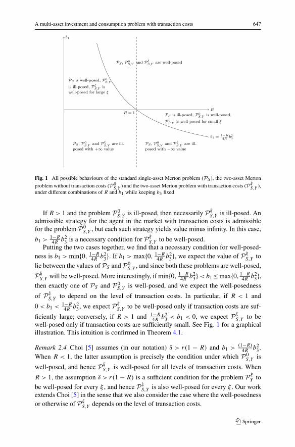
The necessary and sufficient condition for PS to be well-posed is given by b1 > 0.(If R < 1 and b1 ≤ 0, then there is an admissible strategy which yields infinite dis-counted expected utility of consumption. This strategy typically defers consumptionfrom the present to the future, in order to build up large wealth reserves. If R > 1and b1 ≤ 0, then every admissible strategy yields a discounted expected utility ofconsumption of minus infinity.) The necessary and sufficient condition for P0

S,Y to be

well-posed is b1 > 1−R4R

b23.

If R < 1 and the problem PS is ill-posed, then necessarily PξS,Y is ill-posed. An

investor may simply liquidate his initial position in Y and then follow any admissiblestrategy for the single-asset problem involving S alone which yields infinite expecteddiscounted utility. (If necessary, we may consider a sequence of admissible strategiesinvolving investing in S alone.) In this case, b1 > 0 is a necessary condition for Pξ

S,Y

to be well-posed.

4If b3 = 0, the agent chooses never to invest in the illiquid asset. In this case, the agent closes any initialposition in Y at time zero, and thereafter the problem reduces to a standard Merton problem with the singlerisky asset S and no transaction costs.


Fig. 1 All possible behaviours of the standard single-asset Merton problem (PS ), the two-asset Merton

problem without transaction costs (P0S,Y

) and the two-asset Merton problem with transaction costs (PξS,Y

),under different combinations of R and b1 while keeping b3 fixed

If R > 1 and the problem P0S,Y is ill-posed, then necessarily Pξ

S,Y is ill-posed. Anadmissible strategy for the agent in the market with transaction costs is admissiblefor the problem P0

S,Y , but each such strategy yields value minus infinity. In this case,

b1 > 1−R4R

b23 is a necessary condition for Pξ

S,Y to be well-posed.Putting the two cases together, we find that a necessary condition for well-posed-

ness is b1 > min{0, 1−R4R

b23}. If b1 > max{0, 1−R

4Rb2

3}, we expect the value of PξS,Y to

lie between the values of PS and P0S,Y , and since both these problems are well-posed,

PξS,Y will be well-posed. More interestingly, if min{0, 1−R

4Rb2

3} < b1≤ max{0, 1−R4R

b23},

then exactly one of PS and P0S,Y is well-posed, and we expect the well-posedness

of PξS,Y to depend on the level of transaction costs. In particular, if R < 1 and

0 < b1 < 1−R4R

b23, we expect Pξ

S,Y to be well-posed only if transaction costs are suf-

ficiently large; conversely, if R > 1 and 1−R4R

b23 < b1 < 0, we expect Pξ

S,Y to bewell-posed only if transaction costs are sufficiently small. See Fig. 1 for a graphicalillustration. This intuition is confirmed in Theorem 4.1.

Remark 2.4 Choi [5] assumes (in our notation) δ > r(1 − R) and b1 >(1−R)

4Rb2

3.When R < 1, the latter assumption is precisely the condition under which P0

S,Y is

well-posed, and hence PξS,Y is well-posed for all levels of transaction costs. When

R > 1, the assumption δ > r(1 − R) is a sufficient condition for the problem PξY to

be well-posed for every ξ , and hence PξS,Y is also well-posed for every ξ . Our work

extends Choi [5] in the sense that we also consider the case where the well-posednessor otherwise of Pξ

S,Y depends on the level of transaction costs.


Remark 2.5 In this paper, we assume there are just two risky assets, and that transac-tion costs are payable on just one of them. More generally, we may have several liq-uid assets on which no transaction costs are payable, provided the model includes nomore than one risky asset which is subject to transaction costs. Although the equationfor the dynamics of the wealth in liquid assets is then more complicated, the problemreduces to a univariate problem in which the state variable is the ratio of wealth in theasset on which transaction costs are payable to liquid wealth; moreover, after scalingfor paper wealth, the HJB equation for the value function, see (3.3) below, is identicalto the case of two risky assets which we study. See Evans et al. [11, Sect. 2.1] andBichuch and Guasoni [2, Sect. 3.4] for a discussion of the multi-asset case and howit may simplify.

3 Heuristic derivation of a free boundary value problem

Inspired by the analysis in the classical case involving a single risky asset only, wepostulate that the value function has the form

V (x, y, θ) = ϒ(x + yθ)1−R

1 − RG

(yθ

x + yθ

)(3.1)

for some strictly positive function G to be determined and ϒ = bR4 RR , a convenient

scaling constant which helps to simplify the HJB equation.Write p := yθ

x+yθ. As in the single-asset case (see Hobson et al. [14]), outside the

no-transaction region, it is straightforward to deduce the form of G to be

G(p) ={

A∗(1 + λp)1−R, − 1λ

≤ p < p∗,A∗(1 − γp)1−R, p∗ < p ≤ 1

γ,

(3.2)

for some positive constants A∗ and A∗ to be determined.Now we consider the no-transaction region. We expect the process

Mt :=∫ t

0e−δs C1−R

s

1 − Rds + e−δtV (Xt , Yt ,�t )

to be a supermartingale in general, and a martingale under the optimal strategy. Sup-pose V is C2,2,1 and strictly increasing and concave in x. Using Itô’s lemma and thenmaximising the drift term of M with respect to C and �, we can formally obtain theHJB equation over the no-transaction region as

R

1 − RV

1−1/Rx + rxVx + αyVy + η2

2y2Vyy − (βVx + ηρyVxy)

2

2Vxx

− δV = 0. (3.3)

Our initial objective is to simplify (3.3). First, (3.1) can be used to reduce (3.3) toa second order, nonlinear equation for G = G(p). Then, away from p = 1, we set5

5The assumption b3 > 0 means that the agent would like to hold positive quantities of the illiquid asset,and that the no-transaction wedge is contained in the half-space {p > 0}. To allow b3 < 0, it is necessary toconsider p < 0. This case can be incorporated into the analysis by incorporating an extra factor of sgn(p)

into the definition of h, so that h(p) = sgn(p(1 − p))|1 − p|R−1G(p). This then leads to extra cases,but no new mathematics, and the problem can still be reduced to solving n′ = O(q,n) where O is givenby (3.6), but now for q < 0.


h(p) = sgn(1−p)|1−p|R−1G(p), w(h) = p(1−p)dhdp

, W(h) = w(h)(1−R)h

, N = W−1

(the inverse of W ) and n(q) = |N(q)|−1/R|1−q|1−1/R . Then6 the HJB equation (3.3)can be reduced to

0 = n(q)

b4− δ + r(1 − R)(1 − q) + α(1 − R)q + η2

2(1 − R)

(qw′(N(q)

) − q)

− 1 − R

2

(β(1 − q) − ηρ(qw′(N(q)) − (1 − R)q))2

qw′(N(q)) + (2R − 1)q − R. (3.4)

Details of the algebra behind the transformation can be found in [14].After multiplying through by the denominator of the last term, this can be viewed

as a quadratic equation in qw′(N(q)). We want the root corresponding to Vxx < 0.This is equivalent to

1

1 − Rp2G′′(p) + 2R

1 − RpG′(p) − RG(p) < 0, (3.5)

which can be restated as qw′(N(q)) + (2R − 1)q − R < 0.From the relationships between w, W , N and n, we have

n′(q)

n(q)= 1 − R

R(1 − q)− 1

R

N ′(q)

N(q)= 1 − R

R(1 − q)− 1 − R

R

q

qw′(N(q)) − (1 − R)q2.

After some algebra, we arrive at the ODE n′(q) = O(q,n(q)), where

O(q,n) = (1 − R)n

R(1 − q)− 2(1 − R)2qn/R

K(q,ϕ(q,n),E(q))(3.6)

with E(q)2 := 4R2(1 − R)2(b2 − 1)(1 − q)2 and

ϕ(q,n) := n − b1 + (1 − R)(b3 − 2R)q + (2 − b2)R(1 − R),

K(q,φ,E) := 2(1 − R)(1 − q)((1 − R)q + R

) − φ − sgn(1 − R)

√φ2 + E2.

(3.7)

Note that the sign in front of the square root in (3.7) comes from the choice of rootfor qw′(N(q)) in (3.4) corresponding to concavity of V .

Define the quadratic function

m(q) := R(1 − R)q2 − b3(1 − R)q + b1

and the algebraic function

�(q) := m(q) + (1 − R)q(1 − q) + (b2 − 1)R(1 − R)q

(1 − R)q + R.

6The key transformation is to set w(h) = p(1 − p) dhdp

. This has the effect of changing the independentvariable, and more importantly reducing the equation to a first order equation.


Note that m has a turning point (a minimum if R < 1 and a maximum if R > 1) at

qM := b32R

, and set mM := m(qM) = b1 − b23(1−R)

4R. The lemma below gives the key

properties of O .

Lemma 3.1 1) O(q,n) can be extended to q = 1 on {(1 − R)n < (1 − R)�(1)} bycontinuity.

2) O(q,n) = 0 if and only if n = m(q).3) For given R and q , the sign of O(q,n) depends only on the signs of n − m(q)

and �(q) − n.

Now we apply the same transformations on the purchase and sale region. For− 1

λ� p < p∗, we have G(p) = A∗ (1 + λp)1−R as given by (3.2). Then

w(h) = p(1 − p)dh

dp= p(1 − p)(1 − R)h

(λ

1 + λp+ 1

1 − p

)

= (1 − R)h

(p(1 + λ)

1 + λp

)

and |1 − W(h)| = |1−p|1+λp

= (A∗|h| )1/(1−R). It follows that n(q) = (A∗)−1/R . This ex-

pression holds for − 1λ� p < p∗, for which q = W(h) = (1+λ)p

1+λp. The equivalent

range in q is thus given by q < q∗ := (1+λ)p∗1+λp∗ . Similarly, on the sale region, we have

n(q) = (A∗)−1/R for q > q∗ := (1−γ )p∗1−γp∗ .

The C2,2,1 smoothness of the original value function V translates into C1 smooth-ness of the transformed value function n. Hence we are looking for a positive, contin-uously differentiable function n and boundary points (q∗, q∗) solving n′ = O(q,n)

on {q ∈ (q∗, q∗)} with n(q) = (A∗)−1/R for q ≤ q∗ and n(q) = (A∗)−1/R forq ≥ q∗. First order smoothness of n at the boundary points forces that we musthave n′(q∗) = n′(q∗) = 0. But by Lemma 3.1, n′(q) = O(q,n(q)) = 0 if and onlyif n(q) = m(q). Hence the free boundary points must be given by the q-coordinateswhere n intersects the quadratic m. The free boundary value problem now becomessolving n′(q) = O(q,n(q)) on {q ∈ (q∗, q∗)} subject to n(q∗) = m(q∗) as well asn(q∗) = m(q∗).

Recall the definition of the round-trip transaction cost ξ = λ+γ1−γ

> 0. Supposefor now that 1 /∈ [p∗,p∗] and in turn 1 /∈ [q∗, q∗]. Exploiting the relationshipsq∗ = (1+λ)p∗

1+λp∗ and q∗ = (1−γ )p∗1−γp∗ , we have

ln(1 + ξ) = ln(1 + λ) − ln(1 − γ ) =∫ p∗

p∗

dp

p(1 − p)−

∫ q∗

q∗

dq

q(1 − q).

Then, applying the definitions of w, N and O and using

∫ p∗

p∗

dp

p(1 − p)=

∫ h∗

h∗

dh

w(h)=

∫ q∗

q∗

N ′(q) dq

(1 − R)qN(q)


and

O(q,n(q))

n(q)= n′(q)

n(q)= 1 − R

R(1 − q)− 1

R

N ′(q)

N(q),

we have

ln(1 + ξ) =∫ q∗

q∗

(− R

q(1 − R)

O(q,n(q))

n(q)

)dq. (3.8)

Hence the required solution from the free boundary value problem is the one suchthat (3.8) holds.

If 1 ∈ [p∗,p∗] or equivalently 1 ∈ [q∗, q∗], the two integrals∫ p∗p∗

dpp(1−p)

and∫ q∗q∗

dqq(1−q)

are not well defined. But it can be shown that (3.8) still holds by using

a limiting argument.To summarise, we are interested in solving the following free boundary value

problem.

Problem 3.2 Find a positive function n(·) and a pair of boundary points (q∗, q∗)solving

n′(q) = O(q,n(q)

), q ∈ [q∗, q∗], (3.9)

n(q∗) = m(q∗), n(q∗) = m(q∗), (3.10)

subject to (3.8).

In Sect. 5, we distinguish several different cases and discuss how to construct thesolution (n(·), q∗, q∗) in each of these cases. The switch of coordinate from p = yθ

x+yθ

to q is, at one level, purely a mathematical simplification. But the quantities q∗, q∗indeed have an important interpretation as the critical proportion of wealth investedin the illiquid asset when the position is evaluated using the ask or bid price. We shallalso see in Sect. 5 that the values of mM = m(qM) and max0≤q≤1

�(q)R−1 are crucial in

determining when the problem is ill-posed.

4 Main results

Given a solution (n(·), q∗, q∗) to Problem 3.2, we can reverse the transformationsin Sect. 3 and construct a candidate value function. The key technicality here is todemonstrate that the function we construct is smooth up to the second order andsatisfies a HJB variational inequality. These issues are covered by Appendices Aand B.

The first pair of main results of this paper are summarised in the following twotheorems. For a given set of risk aversion parameter R, discount factor δ and marketparameters r , μ, σ , α, η, ρ, we say the problem is unconditionally well-posed ifthe value function is finite on the interior of the solvency region for all values of thetransaction costs λ ≥ 0 and γ ∈ [0,1) with λ+γ > 0. We say the problem is ill-posed


if the value function is infinite for all λ and γ . We say the problem is conditionallywell-posed if the problem is well-posed for some values of the round-trip transactioncost, but ill-posed for other values.

Let L(q) = b1−�(q)1−R

= (b3 − 1)q + (1 − R)q2 − (b2−1)Rq(1−R)q+R

and define the constantL∗ = max0≤q≤1 L(q). Note that L and L∗ depend on R, b2 and b3, but not on b1. ForR < 1, L is convex on [0,1] and L∗ = max{L(0),L(1)} = (b3 − b2R)+. If R > 1,then L is concave and there is no correspondingly simple expression for L∗, althoughwe have the simple bound L∗ ≥ (b3 − b2R)+.

Theorems 4.1 and 4.3 are proved in Appendix C.

Theorem 4.1 The investment/consumption problem (Problem 2.1) is well-posed ifand only if there is a positive solution to Problem 3.2. In particular, it is

1) unconditionally well-posed if(a) R < 1 and b1 ≥ 1−R

4Rb2

3;(b) R > 1 and b1 ≥ −(R − 1)L∗;

2) ill-posed if(a) R < 1 and b1 ≤ (1 − R)(b3 − b2R)+;(b) R > 1 and b1 ≤ 1−R

4Rb2

3;3) conditionally well-posed if

(a) R < 1 and (1 − R)(b3 − b2R)+ < b1 < 1−R4R

b23; in this case, the problem is

well-posed if and only if ξ > ξ , where ξ is defined in (5.2) below;(b) R > 1 and 1−R

4Rb2

3 < b1 < −(R − 1)L∗; in this case, the problem is well-posed if and only if ξ < ξ .

Note thatb2

34R

≥ b3 −R > b3 −b2R so that in the case R < 1, we have the inequality1−R4R

b23 > (1 − R)(b3 − b2R).

The condition b1 > (1 − R)(b3 − b2R) simplifies to δ > (1 − R)(α − η2R2 ). Given

the results of [14] on the single-asset case, we have the following corollary.

Corollary 4.2 Suppose R < 1. The problem with risky liquid asset and illiquid riskyasset is ill-posed (for all values of transaction costs) if and only if the problem withthe liquid asset alone is ill-posed or the problem with risky liquid asset omitted isill-posed (for all values of transaction costs).

When R < 1, it is clear that if PS is ill-posed or if PξY is ill-posed, then Pξ

S,Y isill-posed; so the main content of Corollary 4.2 is the ‘only if’ statement.

The next theorem links the solution of the free boundary value problem and thatof the optimal investment/consumption problem.

Theorem 4.3 Suppose the parameters are such that Problem 2.1 is well-posed and(n(·), q∗, q∗) is the solution to the free boundary value problem (Problem 3.2). Set

V C(x, y, θ) =(

b1

Rb4

)−R(x + yθ)1−R

1 − RGC

(yθ

x + yθ

),


where GC is a C2 function constructed from n as described in Proposition A.1 of Ap-pendix A. Then V C = V where V is the value function of the investment/consumptionproblem defined in (2.1). The purchase and sale boundaries of the illiquid asset aregiven by

p∗ = q∗1 + λ(1 − q∗)

, p∗ = q∗

1 − γ (1 − q∗). (4.1)

Purchase of the illiquid asset occurs whenever yθx+yθ

= p < p∗. Using (4.1), this

condition can be rewritten as yθ(1+λ)x+yθ(1+λ)

< q∗. Hence q∗ can also be viewed as acritical threshold at which purchase occurs, but now the illiquid asset is valued at theask price y(1 +λ) instead of the pre-transaction cost price y. A similar interpretationholds for q∗.

5 Solutions to the free boundary value problem

In this section, we discuss the key features of the solutions to Problem 3.2.Recall that (qM,mM) is the extreme point of the quadratic m (a minimum when

R < 1 and a maximum when R > 1) with qM = b32R

> 0. The key analytical propertiesof the problem only depend on the signs of the four parameters b1, 1 − R, mM ,max0≤q≤1(R − 1)�(q). We classify six different cases. In the analysis of the cases,we make extensive use of the properties of O given in Lemma 3.1 and Lemma D.1of Appendix D.

We parametrise the family of solutions to (3.9) by the left boundary point. Fix u

such that m(u) ≥ 0 and denote by (nu(q))q�u the solution to the initial value problem

n′(q) = O(q,n(q)

), n(u) = m(u).

Let ζ(u) = inf{q � u : (1 − R)nu(q) < (1 − R)m(q)} denote where nu first crossesm to the right of u. Define

�(u) = exp

(∫ ζ(u)

u

(− R

q(1 − R)

O(q,nu(q))

nu(q)

)dq

)− 1. (5.1)

Let F(q,n) = O(q,n)n

and set F(q,0) = limn↓0 F(q,n). Let p− ≤ p+ be the roots ofm(q) = 0. Set

ξ := exp

(−

∫ p+

p−

R

q(1 − R)F(q,0) dq

)− 1. (5.2)

Lemma 5.1 1) Suppose R < 1.(a) Suppose b1 ≥ 1−R

4Rb2

3. Then � is a strictly decreasing, continuous mapping� : (0, qM ] → [0,∞) with �(0+) = +∞ and �(qM) = 0.

(b) Suppose (1 − R)(b3 − b2R)+ < b1 ≤ 1−R4R

b23. Then � is a strictly decreas-

ing, continuous mapping � : (0,p−] → [ξ,∞) with �(0+) = +∞ and �(p−) = ξ .Moreover, limu↑p− nu(·) = 0 and limu↑p− ζ(u) = p+.


2) Suppose R > 1.(a) Suppose b1 ≥ −L∗(R−1). Then � is a strictly decreasing, continuous map-

ping � : (p−, qM ] → [0,∞) with �(p−+) = +∞ and �(qM) = 0.(b) Suppose 1−R

4Rb2

3 < b1 < −L∗(R − 1). Then � is a strictly decreasing, con-tinuous mapping � : (p−, qM ] → [0, ξ) with �(p−) = ξ and �(qM) = 0. Moreover,limu↓p− nu(·) = 0 and limu↓p− ζ(u) = p+.

Lemma 5.1 is proved in Appendix D.

5.1 The cases

5.1.1 Case 1: R < 1 and mM ≥ 0. Equivalently, this may be stated as R < 1 andb1 ≥ 1−R

4Rb2

3

For any initial value u ∈ (0, qM),

m′(u) < 0 = O(u,m(u)

) = O(u,nu(u)

) = n′u(u).

Thus nu(q) must initially be larger than m(q) for q being close to u. It can be checkedthat O(q,n) is negative on the set

{(q,n) : 0 < q � 1,m(q) < n < �(q)} ∪ {(q,n) : q > 1, n > m(q)}(see part 4 of Lemma D.1 in Appendix D). Also, nu(q) cannot cross �(q) from belowon {0 < q � 1} since limn↑�(q) O(q,n) = −∞; see for example (D.4). By consider-ing the sign of O(q,n), we conclude that nu must be decreasing until it crosses m.This guarantees the finiteness of ζ(u), and the triple (nu(·), u, ζ(u)) represents onepossible solution to problem (3.10). Notice that the family of solutions (nu(·))0<u<qM

cannot cross, and thus nu(q) is decreasing in u. The solutions corresponding to initialvalues u = 0 and u = qM can be understood as the appropriate limits of a sequenceof solutions.

Although O(q,n) has singularities at q = 1 and n = �(q), a well-defined limitO(q,n) exists on {(q,n) : q = 1, n < �(1)} and {(q,n) : q > 1, n = �(q)} (see part 3of Lemma D.1 in Appendix D). Hence there exists a continuous modification ofO(q,n), and a solution nu can actually pass through these singularity curves. SeeFig. 2(a) for some examples.

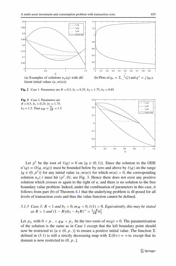
From the analysis leading to (3.8), the correct choice of u should satisfy ξ = �(u).From Lemma 5.1, for every given level of round-trip transaction cost ξ , there existsa unique choice of the left boundary point given by u∗ = �−1(ξ), and then the de-sired solution to the free boundary value problem is given by (nu∗(·), u∗, ζ(u∗)).Figure 2(b) gives the plots of �−1(ξ) and ζ(�−1(ξ)) representing the boundaries(q∗, q∗) under different levels of transaction costs.

5.1.2 Case 2: R < 1 and either b1 ≤ 0 or b1 > 0,mM < 0, �(1) ≤ 0. Equivalently,this may be stated as R < 1 and b1 ≤ (1 − R)(b3 − b2R)+

If b1 ≤ 0, then m is negative on (0, qM ] and there can be no nonnegative solutions ton′ = O(q,n) with n(u) = m(u) for u ∈ (0, qM ].


Fig. 2 Case 1. Parameters are R = 0.5, b1 = 0.25, b2 = 1.75, b3 = 0.85

Fig. 3 Case 2. Parameters areR = 0.5, b1 = 0.25, b2 = 1.75,

b3 = 1.5. Then qM = b32R

= 1.5

Let p� be the root of �(q) = 0 on {q ∈ (0,1)}. Since the solution to the ODEn′(q) = O(q,n(q)) must be bounded below by zero and above by �(q) on the range{q ∈ (0,p�)} for any initial value (u,m(u)) for which m(u) > 0, the correspondingsolution nu(·) must hit (p�,0); see Fig. 3. Hence there does not exist any positivesolution which crosses m again to the right of u, and there is no solution to the freeboundary value problem. Indeed, under the combination of parameters in this case, itfollows from part (b) of Theorem 4.1 that the underlying problem is ill-posed for alllevels of transaction costs and thus the value function cannot be defined.

5.1.3 Case 3: R < 1 and b1 > 0,mM < 0, �(1) > 0. Equivalently, this may be statedas R < 1 and (1 − R)(b3 − b2R)+ < 1−R

4Rb2

3

Let p± with 0 < p− < qM < p+ be the two roots of m(q) = 0. The parametrisationof the solution is the same as in Case 1 except that the left boundary point shouldnow be restricted to {u ∈ (0,p−)} to ensure a positive initial value. The function �

defined in (5.1) is still a strictly decreasing map with �(0+) = +∞ except that itsdomain is now restricted to (0,p−].


Fig. 4 Case 3. Parameters are R = 0.5, b1 = 0.25, b2 = 1.75, b3 = 1.2

Unlike Case 1, we now only consider �−1(ξ) on the range {ξ ∈ (ξ ,∞)}. For sucha given high level of round-trip transaction cost, the required left boundary pointis given by u∗ = �−1(ξ) and u∗ = ζ(u∗); see Fig. 4. In this case, the problem isconditionally well-posed, i.e., it is well-posed only for a sufficiently high level oftransaction cost.

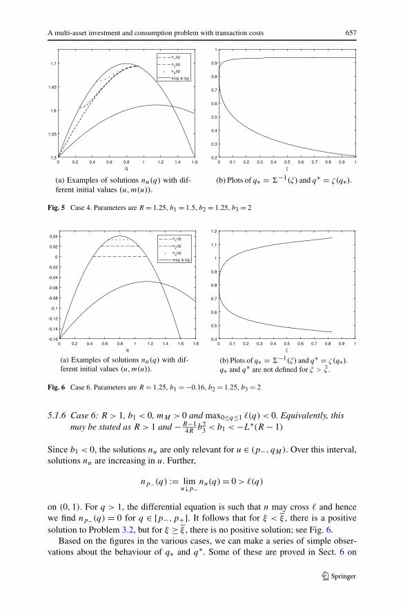
5.1.4 Case 4: R > 1 and either b1 ≥ 0 or both b1 < 0 and max0≤q≤1 �(q) ≥ 1.Equivalently, this may be stated as R > 1 and b1 ≥ −L∗(R − 1)

Suppose first b1 ≥ 0. In this case, the quadratic m is positive on (0, qM ], has a positivemaximum at (qM,mM) and m(q) > �(q) on {q ∈ (0,1)}. By checking the sign ofO(q,n) in case of R > 1, one can verify that the solution nu of the initial valueproblem is always increasing for any choice of left boundary point u ∈ (0, qM). Inthis case, the family of solutions is increasing in u. The solution nu(q) crosses m(q)

from below at ζ(u) = inf{q � u : nu(q) > m(q)}. The correct choice of u is againthe one solving ξ = �(u), where � is defined in (5.1). As in Case 1, the function �

is onto from (0, qM ] to [0,∞), and hence u∗ = �−1(ξ) always exists uniquely forany ξ ; see Fig. 5.

Now suppose that −L∗(R − 1) ≤ b1 < 0, from which it follows that � has a rootp� ∈ (0,1]. As before, we can define a nonnegative, increasing solution nu for anyu ∈ (p−, qM) which crosses m(q) from below at ζ(u). This family of solutions isincreasing in u and each member is bounded below by �(q). Let np− be given bynp−(q) = limu↓p− nu(q). Then np−(q) = 0 for p− < q ≤ p�, but np−(q) > �(q)

for p� < q ≤ 1. By Lemma 5.1, � is onto from (p−, qM ] to [0,∞) and henceu∗ = �−1(ξ) always exists for any ξ .

5.1.5 Case 5: R > 1 and mM ≤ 0. Equivalently, this may be stated as b1 ≤ −R−14R

b23

These parameter values are such that m is nonpositive on (0, qM ] and there can be nopositive solution to n′ = O(q,n) with initial condition n(u) = m(u).


Fig. 5 Case 4. Parameters are R = 1.25, b1 = 1.5, b2 = 1.25, b3 = 2

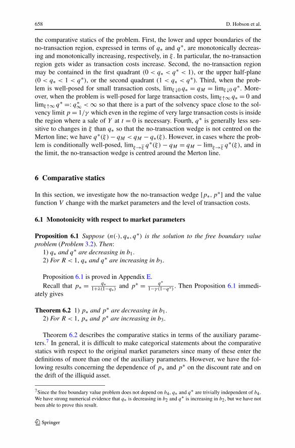
Fig. 6 Case 6. Parameters are R = 1.25, b1 = −0.16, b2 = 1.25, b3 = 2

5.1.6 Case 6: R > 1, b1 < 0, mM > 0 and max0≤q≤1 �(q) < 0. Equivalently, thismay be stated as R > 1 and −R−1

4Rb2

3 < b1 < −L∗(R − 1)

Since b1 < 0, the solutions nu are only relevant for u ∈ (p−, qM). Over this interval,solutions nu are increasing in u. Further,

np−(q) := limu↓p−

nu(q) = 0 > �(q)

on (0,1). For q > 1, the differential equation is such that n may cross � and hencewe find np−(q) = 0 for q ∈ [p−,p+]. It follows that for ξ < ξ , there is a positivesolution to Problem 3.2, but for ξ ≥ ξ , there is no positive solution; see Fig. 6.

Based on the figures in the various cases, we can make a series of simple obser-vations about the behaviour of q∗ and q∗. Some of these are proved in Sect. 6 on


the comparative statics of the problem. First, the lower and upper boundaries of theno-transaction region, expressed in terms of q∗ and q∗, are monotonically decreas-ing and monotonically increasing, respectively, in ξ . In particular, the no-transactionregion gets wider as transaction costs increase. Second, the no-transaction regionmay be contained in the first quadrant (0 < q∗ < q∗ < 1), or the upper half-plane(0 < q∗ < 1 < q∗), or the second quadrant (1 < q∗ < q∗). Third, when the prob-lem is well-posed for small transaction costs, limξ↓0 q∗ = qM = limξ↓0 q∗. More-over, when the problem is well-posed for large transaction costs, limξ↑∞ q∗ = 0 andlimξ↑∞ q∗ =: q∗∞ < ∞ so that there is a part of the solvency space close to the sol-vency limit p = 1/γ which even in the regime of very large transaction costs is insidethe region where a sale of Y at t = 0 is necessary. Fourth, q∗ is generally less sen-sitive to changes in ξ than q∗ so that the no-transaction wedge is not centred on theMerton line; we have q∗(ξ) − qM < qM − q∗(ξ). However, in cases where the prob-lem is conditionally well-posed, limξ→ξ q∗(ξ) − qM = qM − limξ→ξ q∗(ξ), and inthe limit, the no-transaction wedge is centred around the Merton line.

6 Comparative statics

In this section, we investigate how the no-transaction wedge [p∗,p∗] and the valuefunction V change with the market parameters and the level of transaction costs.

6.1 Monotonicity with respect to market parameters

Proposition 6.1 Suppose (n(·), q∗, q∗) is the solution to the free boundary valueproblem (Problem 3.2). Then:

1) q∗ and q∗ are decreasing in b1.2) For R < 1, q∗ and q∗ are increasing in b3.

Proposition 6.1 is proved in Appendix E.Recall that p∗ = q∗

1+λ(1−q∗) and p∗ = q∗1−γ (1−q∗)

. Then Proposition 6.1 immedi-ately gives

Theorem 6.2 1) p∗ and p∗ are decreasing in b1.2) For R < 1, p∗ and p∗ are increasing in b3.

Theorem 6.2 describes the comparative statics in terms of the auxiliary parame-ters.7 In general, it is difficult to make categorical statements about the comparativestatics with respect to the original market parameters since many of these enter thedefinitions of more than one of the auxiliary parameters. However, we have the fol-lowing results concerning the dependence of p∗ and p∗ on the discount rate and onthe drift of the illiquid asset.

7Since the free boundary value problem does not depend on b4, q∗ and q∗ are trivially independent of b4.We have strong numerical evidence that q∗ is decreasing in b2 and q∗ is increasing in b2, but we have notbeen able to prove this result.


Corollary 6.3 p∗ and p∗ are decreasing in δ. If R < 1, then p∗ and p∗ are increas-ing in α.

The corollary confirms the intuition that as the return on the illiquid asset in-creases, it becomes more valuable and the agent elects to buy the illiquid asset sooner,and to sell it later. Moreover, as his discount parameter increases, he wants to con-sume wealth sooner, and since consumption takes place from the cash account, heelects to keep more of his wealth in liquid assets, and less in the illiquid asset.

Now we consider the equivalent cash value of the holdings in the illiquid asset. Wecompare the agent with holdings in the illiquid asset to an otherwise identical agent(same risk aversion and discount parameter, and trading in the financial market withbond and risky asset with price S) who has a zero initial endowment in the illiquidasset and is precluded from taking any positions in the illiquid asset.

Consider the market without the illiquid asset. For an agent operating in this mar-ket, a consumption/investment strategy is admissible for initial wealth x > 0 (wewrite (C = (Ct )t≥0,� = (�t )t≥0) ∈ AW(x)) if C and � are progressively measur-able and the resulting wealth process X = (Xt )t≥0 is nonnegative for all t . Here X

solves dXt = r(Xt − �t)dt + �t

StdSt − Ct dt subject to X0 = x. Let W = W(x) be

the value function for a CRRA investor, i.e.,

W(x) = sup(C,�)∈AW (x)

E

[∫ ∞

0e−δt C1−R

t

1 − Rdt

].

The problem of finding W is a classical Merton consumption/investment problemwithout transaction costs. For the problem to be well-posed, we require that b1 > 0.

For the rest of this section, we assume that b1 > 0. We find W(x) = ( b1b4R

)−R x1−R

1−R.

Define C = C(yθ;x) to be the certainty equivalent value of holding the illiquidasset, i.e., the cash amount which the agent with liquid wealth x and θ units of illiq-uid asset with current price y, trading in the market with transaction costs, wouldexchange for his holdings of the illiquid asset if after this exchange he is not al-lowed to trade in the illiquid asset. (We assume there are no transaction costs onthis exchange, but they can be easily added if required.) Then C = C(yθ;x) solvesW(x + C) = V (x, y, θ) which gives C= C(yθ;x) = (x+yθ)b

R/(1−R)

1 G(p)1/(1−R)−x.Theorem 6.4 is proved in Appendix E.

Theorem 6.4 Suppose b1 > 0.1) (1 − R)bR

1 G is decreasing in b1.2) (1 − R)G is increasing in b3.

Corollary 6.5 Suppose b1 > 0. C is decreasing in δ and increasing in α.

Both these monotonicities are intuitively natural. For the monotonicity in α, sincethe agent only ever holds long8 positions in the illiquid asset, we expect him to benefit

8Note that if he starts with a solvent initial portfolio, but a negative holding in the illiquid asset, then theagent makes an instantaneous transaction at time zero to make his holding positive.


from an increase in the return and hence the future price of the illiquid asset. (Notethat some care is needed in making this argument precise. Part of the optimal strategyis to sometimes purchase units of the illiquid asset, and this will potentially be morecostly as α increases since by Corollary 6.3, p∗ is increasing in α and thus typically,the agent may expect to make purchases of the illiquid asset at a higher price.) For themonotonicity in δ, we note that increases in δ tilt consumption towards the presentwith the effect that the investor has less wealth at future times with which to benefitfrom the growth of the expected value of the risky asset.

6.2 Monotonicity with respect to transaction costs

From the discussion in Sect. 5, we have seen that transformed boundaries only dependon the round-trip transaction cost ξ . In particular, q∗ and q∗ are respectively strictlydecreasing and increasing in ξ and hence the Merton line is included in [q∗, q∗], theno-transaction region with its critical boundaries measured in prices after transactioncosts. However, the purchase/sale boundaries in the original scale still depend on theindividual costs of purchase and sale. Write

p∗(λ, γ ) = q∗(ξ)

1 + λ(1 − q∗(ξ)), p∗(λ, γ ) = q∗(ξ)

1 − γ (1 − q∗(ξ))

and recall that ξ = λ+γ1−γ

. We have

dp∗dγ

= ∂p∗∂q∗

∂q∗∂ξ

∂ξ

∂γ= 1 + λ

(1 − γ )2

1 + λ

(1 + λ(1 − q∗))2

∂q∗∂ξ

< 0

so that the critical ratio of wealth in the illiquid asset to paper wealth at which theagent purchases more illiquid asset is decreasing in the transaction cost on sales.However, the dependence of the critical ratio p∗ at which purchases occur on thetransaction cost on purchases is ambiguous in sign; indeed,

dp∗dλ

= ∂p∗∂λ

+ ∂p∗∂q∗

∂q∗∂ξ

∂ξ

∂λ= − q∗(1 − q∗)

(1 + λ(1 − q∗))2+ 1

1 − γ

1 + λ

(1 + λ(1 − q∗))2

∂q∗∂ξ

is not necessarily negative, for we may have q∗ > 1. Indeed, the Merton line can lieoutside the no-transaction region [p∗,p∗], and the boundaries of this region need notbe monotonic in the transaction cost parameters. In the single-asset case, the locationof the no-transaction region is discussed by Shreve and Soner [23], and the issues areconsidered further in Hobson et al. [14].

7 Conclusion

In this paper, we study the Merton investment and consumption problem under trans-action costs with two risky assets in the special case where transaction costs arepayable on only one of the risky assets. The presence of the second risky asset, whichmay be used for hedging and investment purposes, makes the problem significantly


more complicated than the single-risky-asset case, but we can extend the methodsof [14] to give a complete solution. Indeed, up to evaluating an integral of a knownalgebraic function, we can determine exactly when the problem is well-posed, andup to solving a free boundary value problem for a first order differential equation, wecan determine the boundaries of the no-transaction wedge.

At the heart of our analysis is this free boundary value problem. Although theutility maximisation problem depends on many parameters describing the agent (hisrisk aversion and discount rate), the market (the interest rate and the drifts, volatilitiesand correlations of the traded assets) and the frictions (the transaction costs on salesand purchases), the ODE depends on the risk aversion parameter and just three furtherparameters, and the solution we want can be specified further in terms of the round-trip transaction cost.

Choi et al. [6] and our previous work [14] give a solution to the problem in the caseof a single risky asset. The major issue in [6] and [14] is to understand the solutionof an ODE as it passes through a singular point. In the present paper, the problemis richer and the ODE is more complicated, but in other ways, the analysis is muchsimpler because although the key ODE has singularities, these can be removed.

In the paper, we have assumed a single illiquid asset and just one further riskyasset, but the analysis extends immediately to the case of a single illiquid asset andseveral risky assets on which no transaction costs are payable, at the expense of amore complicated notation. The extension to a model with many risky assets withtransaction costs payable on all of them remains a challenging open problem.

Publisher’s Note Springer Nature remains neutral with regard to jurisdictional claims in published mapsand institutional affiliations.

Open Access This article is distributed under the terms of the Creative Commons Attribution 4.0 Inter-national License (http://creativecommons.org/licenses/by/4.0/), which permits unrestricted use, distribu-tion, and reproduction in any medium, provided you give appropriate credit to the original author(s) andthe source, provide a link to the Creative Commons license, and indicate if changes were made.

Appendix A: Continuity and smoothness of the candidate valuefunction

Suppose there exists a solution (n(·), q∗, q∗) to Problem 3.2 with n being strictlypositive. Define the constants p∗ = q∗

1+λ(1−q∗) and p∗ = q∗1−γ (1−q∗) and the functions

N(q) = sgn(1 − q)n(q)−R|1 − q|R−1, W = N−1 (which is the inverse of N ) andw(h) = (1 − R)hW(h). We should like to construct the candidate value functionGC based on the definition GC(p) = sgn(1 − p)|1 − p|1−Rh(p), where h solvesdhdp

= w(h)p(1−p)

. The main subtlety is that w(h)p(1−p)

is not well defined at p = 1. Nonethe-

less, the definition of GC at p = 1 can be understood in a limiting sense. To thisend, we distinguish two different cases based on whether q∗ − 1 and q∗ − 1 have thesame sign or not, or equivalently whether the no-transaction wedge, plotted in (x, yθ)

space, includes the vertical axis {x = 0} (corresponding to p = 1).


Proposition A.1 (i) Suppose 1 /∈ [p∗,p∗]. Define h(p) via∫ h(p)

N(q∗)

du

w(u)=

∫ p

p∗

du

u(1 − u)(A.1)

on {p∗ � p � p∗}. Then (A.1) is equivalent to∫ N(q∗)

h(p)

du

w(u)=

∫ p∗

p

du

u(1 − u), (A.2)

and (A.2) is an alternative definition of h(p).Let

GC(p) =

⎧⎪⎨⎪⎩

n(q∗)−R (1 + λp)1−R , p ∈ [− 1λ,p∗),

sgn(1 − p)|1 − p|1−Rh(p), p ∈ [p∗,p∗],n(q∗)−R (1 − γp)1−R , p ∈ (p∗, 1

γ].

Then GC is a C2 function on (− 1λ, 1

γ). Moreover, (x+yθ)1−R

1−RGC(

yθx+yθ

) is strictlyincreasing and strictly concave in x.

(ii) Suppose 1 ∈ [p∗,p∗]. Define h(p) via⎧⎨⎩

∫ h(p)

N(q∗)du

w(u)= ∫ p

p∗du

u(1−u), p∗ < p < 1,∫ N(q∗)

h(p)du

w(u)= ∫ p∗

pdu

u(1−u), 1 < p < p∗.

Let

GC(p) =

⎧⎪⎪⎪⎨⎪⎪⎪⎩

n(q∗)−R (1 + λp)1−R , p ∈ [− 1λ,p∗),

sgn(1 − p)|1 − p|1−Rh(p), p ∈ [p∗,p∗] \ {1},n(1)−Re−(1−R)a, p = 1,

n(q∗)−R (1 − γp)1−R , p ∈ (p∗, 1γ]

with a := − ∫ 1q∗

Rq(1−R)

O(q,n(q))n(q)

dq − ln(1 + λ). Then |a| � ln(1 + ξ), and GC is a

C2 function on (− 1λ, 1

γ). Moreover, (x+yθ)1−R

1−RGC(

yθx+yθ

) is strictly increasing andstrictly concave in x.

Proof (i) We have∫ N(q∗)

N(q∗)

du

w(u)−

∫ p∗

p∗

du

u(1 − u)

=∫ q∗

q∗

(N ′(u)

(1 − R)uN(u)− 1

u(1 − u)

)du +

∫ q∗

q∗

du

u(1 − u)−

∫ p∗

p∗

du

u(1 − u)

=∫ q∗

q∗

(− R

u(1 − R)

O(u,n(u))

n(u)

)du − ln(1 + ξ) = 0,

using (3.8), and this establishes the equivalence of (A.1) and (A.2).


Suppose we have a solution (n(·), q∗, q∗) to (3.9) with n being strictly positive.Let GC = GC(p) be defined as at the start of this section. For notational convenience(and to allow us to write derivatives as superscripts), write G as shorthand for GC .

First we check that G is C2. Outside the no-transaction interval, this is immediatefrom the definition, and on (p∗,p∗), it follows from the fact that n and n′ are con-tinuous. This property is inherited by the pair (w,w′) and then on integration by thetrio (h,h′, h′′) and finally (G,G′,G′′).

It remains to check the continuity of G, G′ and G′′ at p∗ and p∗. We prove thecontinuity at p∗; the proofs at p∗ are similar. Using 1−q∗

1−p∗ = 11+λp∗ for the penultimate

equivalence, we have

G(p∗+) = sgn(1 − p∗)|1 − p∗|1−Rh(p∗)

= sgn(1 − p∗)|1 − p∗|1−R sgn(1 − q∗)n(q∗)−R|1 − q∗|R−1

= n(q∗)−R(1 + λp∗)1−R = G(p∗−).

By tracing the definitions of h, w and W , it can be shown that

G(p) − pG′(p)

1 − R= |1 − p|−Rh

(1 − W(h)

)(A.3)

and

p2G′′(p) + 2RpG′(p) − R(1 − R)G(p)

= sgn(1 − p)|1 − p|−(1+R)(w(h)w′(h) + (2R − 1)w(h) − R(1 − R)h

). (A.4)

Then continuity of G′ at p∗ immediately follows from (A.3), where

G(p∗+) − p∗G′(p∗+)

1 − R= h∗(1 − W(h∗))

|1 − p∗|R = G(p∗−) − p∗G′(p∗−)

1 − R.

Continuity of G′′ at p∗ now follows from (A.4) and continuity of G and G′.Now we argue that (x+yθ)1−R

1−RG(

yθx+yθ

) is strictly increasing and strictly concavein x. Outside [p∗,p∗], this is immediate from the definition. On [p∗,p∗], the increas-ing property follows if G(p) − pG′(p)

1−R> 0. But this is trivial since

G(p) − pG′(p)

1 − R= h(1 − W(h))

|1 − p|R = N(q)(1 − q)

|1 − p|R =∣∣∣∣ 1 − q

1 − p

∣∣∣∣R

n(q)−R > 0.

Meanwhile, (x+yθ)1−R

1−RG(

yθx+yθ

) being concave on [p∗,p∗] is equivalent to the condi-tion that qw′(N(q)) + (2R − 1)q − R < 0. But this follows from our choice of rootin (3.7).

(ii) Note that the integrand of∫ q∗q∗

Rq(1−R)

O(q,n(q))n(q)

dq is everywhere negative and

therefore we have existence of∫ 1q∗(− R

q(1−R)O(q,n(q))

n(q)) dq in [0, ln(1 + ξ)]. Hence we

can establish − ln(1 + ξ)� a � ln(1 + ξ).


For p �= 1, the C2 smoothness of G = GC follows as in (i). We focus on the casep = 1. Suppose first that p∗ < 1 < p∗. Continuity of G and G′ at p = 1 can beestablished if we can show that both

limp→1

1

G(p)

(G(p) − pG′(p)

1 − R

)1−1/R

= n(1) (A.5)

and

limp→1

pG′(p)

(1 − R)G(p)= 1 − ea. (A.6)

Substituting (A.6) into (A.5), we recover the given value of G(1).Using (A.3) and the equivalence of p → 1 and q → 1, we have

1

G(p)

(G(p) − pG′(p)

1 − R

)1−1/R

= |h|−1/R|1 − W(h)|1−1/R = n(q) −→ n(1)

and (A.5) holds. For (A.6), we have

1 − W(h(p))

1 − p= (1 − R)h(p) − p(1 − p)h′(p)

(1 − R)(1 − p)h(p)= 1 − pG′(p)

(1 − R)G(p).

Suppose p < 1. Then using the definition of h(p),

0 =∫ h(p)

N(q∗)

du

w(u)−

∫ p

p∗

du

u(1 − u)=

∫ W(h(p))

q∗

N ′(q) dq

(1 − R)qN(q)−

∫ p

p∗

du

u(1 − u)

=∫ W(h(p))

q∗

(N ′(q)

(1 − R)qN(q)− 1

q(1 − q)

)dq

+∫ W(h(p))

q∗

dq

q(1 − q)−

∫ p

p∗

du

u(1 − u)

=∫ W(h(p))

q∗

(− R

u(1 − R)

O(u,n(u))

n(u)

)du −

∫ q∗

p∗

du

u(1 − u)−

∫ p

W(h(p))

dq

q(1 − q)

=∫ W(h(p))

q∗

(− R

u(1 − R)

O(u,n(u))

n(u)

)du − ln

(p

W(h(p))

1 − W(h(p))

1 − p

)

− ln(1 + λ).

Letting p ↑ 1 and using limp→1 W(h(p)) = 1, we obtain limp↑11−W(h(p))

1−p= ea .

A similar calculation for p > 1 leads to limp↓1W(h(p))−1

p−1 = ea . Hence (A.6) holds.As a byproduct, we can establish

limp→1

G′(p) = (1 − R)(1 − ea)G(1) = (1 − R)(1 − ea)n(1)−Re−(1−R)a.


Consider now continuity of G′′ at p = 1. We show that limp→1 G′′(p) exists.

Consider D(p) = ((1−R)G(p)−pG′(p))2

G(p)(p2G′′(p)+2RpG′(p)−R(1−R)G(p)). Then

D(p) = (1 − R)2h(1 − W(h))2

w(h)w′(h) + (2R − 1)w(h) − R(1 − R)h

= (1 − R)(1 − q)2

(1 − R)qN(q)/N ′(q) − (1 − q)(R + (1 − R)q)

= (1 − R)(1 − R − R(1 − q)n′(q)/n(q))

R(R + (1 − R)q)n′(q)/n(q) − R(1 − R)

and

limp→1

D(p) = limq→1

(1 − R)(1 − R − R(1 − q)n′(q)/n(q))

R((R + (1 − R)q)n′(q)/n(q) − (1 − R))

= (1 − R)2

R(n′(1)/n(1) − (1 − R)). (A.7)

Note that n′(1)/n(1) − (1 − R) �= 0 since sgn(n′(1)) = − sgn(1 − R). The limit isthus always well defined and can be used to obtain an expression for limp→1 G′′(p).

Since G is C2 and (3.5) holds for both p < 1 and p > 1, it follows that (3.5) holds

at p = 1 also and (x+yθ)1−R

1−RG(

yθx+yθ

) is concave on [p∗,p∗].Finally, we consider the case where p∗ = 1 or p∗ = 1. Suppose we are in the

former scenario. Then to show the continuity of G at p∗ = 1, it is sufficient toshow that n(q∗)−R (1 + λ)1−R = n(1)−Re−(1−R)a . But q∗ = 1 when p∗ = 1 and thusa = − ln(1 + λ). The above expression then holds immediately. The values of G′(1)

and G′′(1) can again be inferred from (A.6) and (A.7). A similar result follows in thecase p∗ = 1. �

Appendix B: The candidate value function and the HJB equation

We have to verify that the candidate value function given in Proposition A.1 solvesthe HJB variational inequality

min

{− sup

c>0,π

Lc,πV C,−MV C,−NV C

}= 0, (B.1)

where L, M and N are the operators

Lc,πf := c1−R

1 − R− cfx + σ 2

2fxxπ

2 + ((μ − r)fx + σηρfxyy

)π

+ rfxx + αfyy + η2

2fyyy

2 − δf,

Mf := fθ − (1 + λ)yfx, Nf := (1 − γ )yfx − fθ .


Outside the no-transaction region, most of the inequalities in (B.1) follow from theconstruction of V C or direct substitution. We provide a proof of the less trivial resultthat MV C � 0 on the no-transaction region {p ∈ [p∗,p∗]}. The inequality NV C � 0can be proved in an identical fashion. Again writing G as shorthand for GC , we have

MV C = V Cθ − (1 + λ)yV C

x = pV C

θ

((1 + λp)

G′(p)

G(p)− λ(1 − R)

).

Since sgn(V C) = sgn(1 − R), it is necessary and sufficient to show

sgn(1 − R)

((1 + λp)

G′(p)

G(p)− λ(1 − R)

)� 0.

But G(p) = sgn(1 − p)h(p)|1 − p|1−R for p �= 1, and then

G′(p)

G(p)= h′(p)

h(p)− 1 − R

1 − p= w(h)

h(p)p(1 − p)− 1 − R

1 − p= 1 − R

1 − p

(W(h)

p− 1

)

and the required inequality becomes

1 − W(h)

1 − p� 1

1 + λp. (B.2)

We are going to prove (B.2) for p ∈ [p∗,p∗]\{1}. Then MV C � 0 will hold at p = 1as well by smoothness of V C .

By construction, q = W(h(p)). Since W is monotonic and h is monotonic exceptpossibly at p = 1, it follows that q is an increasing function of p. Then, starting fromthe identity

∫ N(q)

N(q∗)dh

w(h)= ∫ p

p∗du

u(1−u)and following the substitutions leading to (3.8),

we find∫ q

q∗

(− R

u(1 − R)

O(u,n(u))

n(u)

)du = −

∫ q

q∗

dv

v(1 − v)+

∫ p

p∗

du

u(1 − u).

Since the expression on the left-hand side is increasing in q , we deduce that we have1

q(1−q)dqdp

� 1p(1−p)

.

Define χ(p) := (1+λ)p1+λp

. Then χ is a solution to the ODE χ ′(p) = �(p,χ(p)),

where �(p,y) = y(1−y)p(1−p)

. Note that χ(p∗) = (1+λ)p∗1+λp∗ = q∗ = q(p∗).

Suppose p∗ < p∗ < 1. Then for p < 1 and in turn q = q(p) = W(h(p)) < 1,we have q ′(p) � �(p,q(p)) and conclude that q(p) � χ(p) for p∗ � p < p∗ � 1.Then 1 − W(h(p)) = 1 − q(p) � 1 − χ(p) = 1−p

1+λpwhich establishes (B.2). If in-

stead 1 < p∗ < p∗, we can arrive at the same result by showing q(p) � χ(p) for1 < p∗ � p and in turn dq

dp� q(q−1)

p(p−1).

It remains to consider the case of p∗ � 1 � p∗. The only issue is that the compari-son of derivatives of q(p) and χ(p) may be not trivial at p = 1 because of the singu-larity in �(p,y). But by direct computation, it can be found that χ ′(1) = 1

1+λ. Mean-

while, q ′(1−) = limp↑11−q(p)

1−p= limp↑1

1−W(h(p))1−p

= ea , and similarly, we have


q ′(1+) = ea . Then q ′(1) is well defined, and moreover since a > − ln(1 + λ), wehave q ′(1) = ea > 1/(1 + λ) = χ ′(1). Together with the fact that q(1) = 1 = χ(1),we must have that q(p) is an upcrossing of χ(p) at p = 1. From this, we concludethat q(p)� χ(p) on {p ∈ [p∗,1)} and χ(p) � q(p) on {p ∈ (1,p∗]}. And (B.2) thenfollows.

Appendix C: Proof of the main results

Proof of Theorems 4.1 and 4.3 We prove the two theorems together. Suppose weare in the well-posed cases. From the analysis in Sect. 5, there exists a solu-tion (n(·), q∗, q∗) to the free boundary value problem with n being strictly pos-itive. By the C2 smoothness of GC , V C is C2,2,1. Moreover, in Appendices Aand B, we have seen that V C is a strictly concave function in x solving theHJB variational inequality (B.1). For R < 1, using the supermartingale property of

Mt := ∫ t

0 e−δs C1−Rs

1−Rds + e−δtV C(Xt , Yt ,�t ), we can establish V ≤ V C following

standard arguments. For R > 1, M may be only a local supermartingale, and fur-ther arguments along the lines of those in Davis and Norman [9] or Tse [25, Ap-pendix 3.D] are needed.

To show V C � V , it is sufficient to demonstrate the existence of an invest-ment/consumption strategy which attains the value V C . Suppose the initial value(x, yθ) is such that yθ

x+yθ= p ∈ [p∗,p∗]. Define feedback controls C∗ = (C∗

t )t�0

and �∗ = (�∗t )t�0, where C∗

t = C∗(Xt , Yt ,�t ) and �∗t = �∗(Xt , Yt ,�t ) with

C∗(x, y, θ) := (V Cx (x, y, θ))− 1

R ,

�∗(x, y, θ) := − (μ − r)V Cx (x, y, θ) + σηρyV C

xy(x, y, θ)

σ 2V Cxx(x, y, θ)

,

and where �∗ = (�∗t )t�0 is a finite-variation, local-time-type strategy of the form

�∗t = θ + �∗

t − ∗t which keeps (Pt ) within (p∗,p∗). Our goal is to show that

the process M∗ = (M∗t )t�0, which is defined as a version of M evolving under

(C∗,�∗,�∗), is a true martingale. The technical delicacy is to show that the local-martingale stochastic integrals

∫ t

0 e−δsσV Cx �∗

s dBs and∫ t

0 e−δsηV Cy YsdWs are in-

deed true martingales. But this can be done following ideas similar to Davis andNorman [9]. Further, it can also be shown that limt→∞ E[e−δtV C(X∗

t , Yt ,�∗t )] = 0.

Then standard arguments lead to V C ≤ V . See Tse [25, Appendix 3.E] for a detailedproof.

Now suppose the initial value (x, yθ) is such that p < p∗. Then consider the strat-egy of purchasing φ = xp∗−(1−p∗)yθ

y(1+λp∗) shares at time zero so that the post-transaction

proportional holding in the illiquid asset is y(θ+φ)x+y(θ+φ)−y(1+λ)φ

= p∗, and there-after following the investment/consumption strategy (C∗,�∗,�∗) as in the caseof {p ∈ [p∗,p∗]}. By its construction, V C(x, y, θ) = V C(x − y(1 + λ)φ, y, θ + φ),and from this we can conclude that V C � V . A similar argument applies for an initialvalue with p > p∗.

Finally, we consider the conditionally well-posed case. From the discussion inSect. 5, it is clear that as long as ξ > ξ , there still exists a solution (n(·), q∗, q∗) to the


free boundary value problem, and thus one can show V C = V by the same argumentas for the unconditionally well-posed cases. Moreover, from Lemma 5.1, we can seethat n(·) ↓ 0 as ξ ↓ ξ , and in turn V C → ∞ from its construction. But V � V C , andthus we conclude that V → ∞ as ξ ↓ ξ . This shows the ill-posedness of the problemat ξ = ξ , and using the monotonicity of V in ξ , this extends to any ξ � ξ . �

Proof of Corollary 4.2 Note that if R < 1, then mM ≤ m(1) ≤ �(1) so that �(1) ≤ 0is necessary and sufficient for both mM < 0 and �(1) ≤ 0. Further, �(1) � 0 is equiv-alent to b3 � b1

1−R+ b2R, and this inequality can be restated as α � 1

2η2R + δ1−R

.But this is exactly the ill-posedness condition in the one-risky-asset case; see [14]or [6]. �

Appendix D: The first order differential equation

The goal of this section is to establish some important results regarding the functionsm(q), �(q) and O(q,n), which then allow us to infer the properties of the solution tothe ODE n′(q) = O(q,n(q)) as in Sect. 5.

Let S ⊆ {(q,n);q > 0, n ≥ 0} be the set

S = {q = 1} ∪{q = R

R − 1

}∪ {n = 0} ∪ {q < 1, (1 − R)n ≥ (1 − R)�(q)}.

On (0,∞) × [0,∞) \ S , define F(q,n) = O(q,n)/n. Extend the definition of F

to (0,∞) × [0,∞) where possible by taking appropriate limits. The lemma belowcollects all the relevant results; it is an extended version of Lemma 3.1.

Lemma D.1 1) (a) For R < 1, �(q) > m(q) on {q ∈ (0,1]}. Moreover, on (0,∞),m crosses � exactly once from below at some point above 1.

(b) For R > 1, m(q) > �(q) on {q ∈ (0,1]}. Moreover, on (0,∞), m either doesnot cross � at all, or touches � exactly once in the open interval (1,R/(R − 1)), orcrosses � twice on (1,R/(R − 1)).

2) For R > 1, F(q,n) is well defined at q = R/(R − 1).3) For n > 0 and (1 − R)n < (1 − R)�(1), F(1, n) is well defined and

F(1, n) := limq→1

F(q,n) = − (1 − R)(n − m(1))

�(1) − n. (D.1)

Also, for q ≤ 1 and R < 1, we have limn↑�(q) F (q,n) = −∞ (and if R > 1,limn↓�(q) F (q,n) = +∞). For q > 1 and R < 1 (and 1 < q < R

R−1 for R > 1), wehave that F(q, �(q)) := limn→�(q) F (q,n) satisfies

F(q, �(q)

) = − 1 − R

R(1 − q)

(q((1 − R)q + R)

((1 − R)q + R)2 + (b2 − 1)R2− 1

). (D.2)

4) F(q,n) = 0 if and only if n = m(q). Moreover,(a) for R < 1:


(i) On {0 < q < 1}, F(q,n) < 0 for m(q) < n < �(q) and F(q,n) > 0 forn < m(q) or n > �(q).

(ii) At q = 1, F(1, n) < 0 for m(1) < n < �(1) and F(1, n) > 0 for n < m(1);F(1, n) is not well defined for n � �(1).

(iii) On {q > 1}, F(q,n) < 0 for n > m(q) and F(q,n) > 0 for n < m(q).(b) for R > 1:

(i) On {0 < q < 1}, F(q,n) > 0 for �(q) < n < m(q) and F(q,n) < 0 forn < �(q) or n > m(q).

(ii) At q = 1, F(1, n) > 0 for �(1) < n < m(1) and F(1, n) < 0 for n > m(1);F(1, n) is not well defined for n � �(1).

(iii) On {1 < q � R/(R − 1)}, F(q,n) < 0 for n > m(q) and F(q,n) > 0 forn < m(q).

(iv) On {q > R/(R − 1)}, F(q,n) < 0 for m(q) < n < �(q) and F(q,n) > 0for n > �(q) or n < m(q).

Before we proceed, we introduce some additional notation:

v(q,n) = ϕ(q,n) − sgn(1 − R)

√ϕ(q,n)2 + E(q)2,

D(q,n) = 2((1 − R)q + R

)(n − m(q)

) − q(v(q,n) − v

(q,m(q)

)),

A(q,n) = D(q,n)

+ (�(q) − n

)(2((1 − R)q + R

) − q(

1 − sgn(1 − R)ϕ√

ϕ2 + E2

)),

(D.3)

where m, �, ϕ and E are defined in Sect. 3. We begin with a useful lemma, whoseproof is a lengthy exercise in algebra and is omitted.

Lemma D.2 O(q,n) has the alternative expression

O(q,n) = − (1 − R)nD(q,n)

2R(1 − q)((1 − R)q + R)(�(q) − n). (D.4)

Proof of Lemma D.1 1) Observe that

�(q) − m(q) = (1 − R)q

((1 − R)q + R)P (q),

where P(q) := Rb2 + (1 − 2R)q − (1 −R)q2. Hence the crossing points of �(q) andm(q) away from q = 0 are given by the roots of P(q) = 0 if such roots exist. Thedesired results can be established easily by studying the quadratic function P(q).

2) The behaviour at q = −R/(1 − R) is only relevant for R > 1; so we write thisas q = R/(R − 1). Note that � explodes at q = R

R−1 . It is sufficient to check that thedenominator of O(q,n) is not equal to zero at q = R/(R − 1). Direct calculation


gives ((1 − R)q + R)(�(q) − n)|q= R

R−1= −(b2 − 1)R2 and hence

2R(1 − q)((1 − R)q + R

)(�(q) − n)

∣∣q= R

R−1= 2R3(b2 − 1)

(R − 1)�= 0.

3) Both the numerator and denominator of F(q,n) are zero at q = 1. L’Hôpital’srule can be applied to calculate limq→1

D(q,n)1−q

to deduce the expression in (D.1) aftersome algebra.

Now consider limn→�(q) F (q,n). Suppose first 0 < q < 1. Then

D(q, �(q)

) = 2(1 − R)q(1 − q)

(((1 − R)q + R

) + R2(b2 − 1)

(1 − R)q + R

),

which is non-zero and has sgn(D(q, �(q))) = sgn(1 − R). It follows that for q < 1and R<1, limn↑�(q)F (q,n) = −∞ and for q<1 and R>1, limn↓�(q)F (q,n) =+∞.

Now suppose q > 1, and if R > 1 that (1 − R)q + R > 0. Then direct evaluationgives D(q, �(q)) = 0.9 In order to determine the value of F(q, �(q)) via L’Hôpital’srule, we need to compute

∂D

∂n= 2

((1−R)q +R

)−q∂v

∂n= 2

((1−R)q +R

)−q

(1− sgn(1 − R)ϕ√

ϕ2 + E2

), (D.5)

and (D.2) follows immediately.4) We prove the results for R < 1. The results for R > 1 can be obtained similarly,

the only issue being that there is an extra case which arises when (1 − R)q + R

changes sign.Note that for fixed q , the ordering of m(q) and �(q) is given by 1). The mono-

tonicity of F in n for q = 1 can be obtained from (D.1).If 0 < q < 1, then since

2((1 − R)q + R

) − q

(1 − sgn(1 − R)ϕ√

ϕ2 + E2

)> 2

((1 − R)q + R

) − 2q

= 2R(1 − q) > 0,

we conclude from (D.5) that D(q,n) is increasing in n. Since D(q,m(q)) = 0,it follows that D(q,n) > 0 for n > m(q) and D(q,n) < 0 for n < m(q). Hence,F(q,n) = 0 if and only if n = m(q), and we have

sgn(F(q,n)

) = − sgn

(D(q,n)

(1 − q)((1 − R)q + R)(�(q) − n)

)

= sgn((

n − m(q))(

n − �(q)))

.

This gives the desired sign properties of F(q,n) on the range {0 < q < 1}.9More generally, D(q, �(q)) = 0 if and only if (1 − q)((1 − R)q + R) < 0. This can be verified withspecial care taken to choose the appropriate square root arising in v(q,n).


Now consider the case q > 1 under which we have D(q, �(q)) = 0. We can com-pute the second derivative of D with respect to n as

∂2D

∂n2= sgn(1 − R)q

E2

(E2 + ϕ2)3/2

and as R < 1, D(q,n) is convex in n. Since D(q,m(q)) = D(q, �(q)) = 0, it followsthat for q > 1, we must have D(q,n) < 0 when n lies between m(q) and �(q), andD(q,n) > 0 otherwise. Thus sgn(D(q,n)) = sgn((n − m(q))(n − �(q))). Then

sgn(F(q,n)

) = sgn

(D(q,n)

�(q) − n

)= − sgn

(n − m(q)

).

Finally, note that F(q,n) can be zero only if n = m(q) or n = �(q). But for q > 1,the limiting expression at n = �(q) is given by 3). Hence F(q,n) = 0 if and only ifn = m(q). �

The following lemma on further properties of F is key in the proofs of the mono-tonicity property of � and in the results on comparative statics.

Lemma D.3 For q ∈ (0,1] and (1 − R)m(q) < (1 − R)n < (1 − R)�(q), and forq > 1 and (1 − R)m(q) < (1 − R)n, we have ∂

∂nF (q,n) � 0.

Proof Direct computation gives

(�(q) − n

)2 ∂

∂n

(D(q,n)

�(q) − n

)= (

�(q) − n)∂D

∂n+ D(q,n) = A(q,n),

where A was defined in (D.3), and in turn ∂∂n

A(q,n) = sgn(1 − R)E(q)2q(�(q)−n)

(ϕ2+E(q)2)3/2 .Hence for q > 0 and R < 1, A(q,n) is increasing in n for n < �(q) and decreasing inn for n > �(q). If R > 1, then A(q,n) is decreasing in n for n < �(q) and increasingin n for n > �(q).

Now we consider the limiting value of A(q,n) as n → ±∞. We can compute

lim(1−R)n→+∞A(q,n) = 2(1 − R)

((1 − R)q + R

)q(1 − q),

lim(1−R)n→−∞A(q,n) = 2R2(1 − R)(b2 − 1)q(1 − q)

(1 − R)q + R

after some algebra.10

Suppose R < 1. For 0 < q < 1, we have that A(q,n) is increasing in n for n < �(q)

and decreasing in n for n > �(q). Since on this range of q , we have

10The case of (1 − R)n → −∞ might appear to be more difficult since v(q,n) does not converge, butcomputation can be facilitated by a useful observation that ϕ(q,n) − n is independent of n.


limn→+∞A(q,n) = 2(1 − R)((1 − R)q + R)q(1 − q) > 0,

limn→−∞A(q,n) = 2R2(1 − R)(b2 − 1)q(1 − q)

(1 − R)q + R> 0,

we conclude that A(q,n) > 0 for all n. If q > 1, then A(q, �(q)) = D(q, �(q)) = 0.But A(q,n) attains its maximum at n = �(q); hence we have A(q,n) � 0 for q > 1.Putting the cases together, (1 − q)A(q,n) ≥ 0 and ∂F

∂n≤ 0. In the special case q = 1,

the result follows from (D.1).Similar arguments can be adopted if R > 1, with extra care taken towards potential

changes of sign at q = RR−1 . �

Proof of Lemma 5.1 We can deduce that �(u) is decreasing by using the monotonic-ity of nu(·) in u and in turn the monotonicity of F(q,n) = O(q,n)

nin n. When qM is

in the domain of �, then limu↑qM�(u) = 0 can be shown easily by using the fact that

qM is a turning point of m(q).We next show that if R < 1 and b1 > 0, then limu↓0 �(u) = +∞. Suppose R < 1

and consider the quadratic function

H(x) = (1 − R)b1(m′(0) − x

) − R(l′(0) − x

)x;

then trivially H(m′(0)) > 0 > H(0). Now choose a constant k such that we havem′(0) < k < α < 0, where α is the negative root of H(x) = 0. Then H(k) > 0 andequivalently k <

(1−R)b1(m′(0)−k)

R(l′(0)−k). Let b(q) = b1 + kq . It is clear from the definition

of D that D(0, b1) = 0. Thus by direct computation, we have

d

dqD(q, b1 + kq)

∣∣∣q=0

= −2Rm′(0) + 2Rk

and

limq↓0

O(q, b(q)

) = −b1(1 − R) ddq

D(q, b1 + kq)|q=0

2R2(�′(0) − k)= (1 − R)b1(m

′(0) − k)

R(l′(0) − k).

Then for all ε > 0, there exists Kε ∈ (0,1) such that for q < Kε , we haveO(q,b(q)) >

(1−R)b1(m′(0)−k)

R(l′(0)−k)− ε. Pick ε such that 0 < ε <

(1−R)b1(m′(0)−k)

R(l′(0)−k)− k.

Then we have O(q,b(q)) > k on {0 < q < Kε} and solutions to n′ = O(q,n) crossb(q) from below. Let ψu = inf(q � u : nu(q) > b(q)). Then for u < q < Kε ∧ ψu,n′

u(q) = O(q,nu(q)) > O(q, b(q)) > k. Moreover, there also exists Km suchthat m′(q) < 1

2 (m′(0) + k) for q < Km. Hence on {u < q < Kε ∧ ψu ∧ Km},we have n′

u(q) − m′(q) > k − 12 (m′(0) + k) = 1

2 (k − m′(0)) =: k > 0 and thennu(q) − m(q) > k(q − u). On the other hand, for ψu < q < Kε ∧ Km,m(q) < b1 + q

2 (m′(0) + k) and hence

nu(q) − m(q) > (b1 + kq) −(b1 + q

2

(m′(0) + k

)) = kq > k(q − u).

We conclude that nu(q) − m(q) > k(q − u) for u < q < Q := Kε ∧ Km.


Hence, using (D.4) and L’Hôpital’s rule,

ln(1 + �(u)

)=

∫ ξ(u)

u

(− R

(1 − R)q

O(q,nu(q))

nu(q)

)dq

>

∫ Q

u

2((1 − R)q + R)(nu(q) − m(q)) − q(v(q,nu(q)) − v(q,m(q)))

2q(1 − q)((1 − R)q + R)(�(q) − nu(q))dq.

Using nu(q) − m(q) > k(q − u), it is not hard to see that the above integrand isbounded below by C(q−u)

q2 on {u < q < Q < Q}, where C and Q are some constantsindependent of u. Then we deduce that

ln(1 + �(u)

)>

∫ Q

u

C(q − u)

q2dq = C

(ln

Q

u+ u

Q− 1

).

Letting u ↓ 0, we conclude that �(u) → ∞.Now suppose R < 1, b1 > 0, mM < 0 and �(1) > 0. The smallest nonnegative

solution nu is for u = p− and then ζ(p−) = p+ and np−(q) = 0 for q ∈ [p−,p+].We have �(p−) = ξ .

Now suppose R > 1. Most of the analysis is the same as for R < 1. However, whenb1 < 0 and mM > 0 (equivalently, b1 > − (R−1)

4Rb2

3), we can only consider solutionsnu for u ∈ [p−, qM ]. The new case arises when max0≤q≤1 �(q) > 0. Then, since �

is a lower bound for n, we have for any u > p− that nu(q) > �(q). In particular,limu↓p− nu(q) > 0 for q > p�. Moreover, by considering the behaviour of F near p�,

we find that∫ p�

F (q,0) dq is infinite and limu↓p− �(u) = ∞. �

Appendix E: Comparative statics

Proof of Proposition 6.1 We only prove Part 2) here. The proof of Part 1) is easierand can be done using the transformation m(q) = m(q) − b1, n(q) = n(q) − b1 and�(q) = �(q) − b1.

Set a(q) = n(q) − m(q). Then the original free boundary value problem becomesto solve a′(q) = O(q,a(q)) subject to a(q∗) = a(q∗) = 0, where

O(q,a) = − (1 − R)(a + m(q))D(q, a + m(q))

2R(1 − q)((1 − R)q + R)(�(q) − m(q) − a)

− 2R(1 − R)q + b3(1 − R).

Observe that �(q)−m(q) = (1 −R)q(1 − q)+ (b2 − 1)R(1 −R)q

(1−R)q+Rdoes not

depend on b3. Further, ϕ(q, a + m(q)) = a + R(1 − R)((1 − q)2 − (b2 − 1)) andv(q,m(q)) = −2R(1 − R)(b2 − 1) are both independent of b3. Hence

D(q, a + m(q)

) = 2((1 − R)q + R

)a − q

(v(q, a + m(q)

) − v(q,m(q)

))


and

O(q, a + m(q)

)a + m(q)

= − (1 − R)D(q, a + m(q))

2R(1 − q)((1 − R)q + R)(�(q) − m(q) − a)

are independent of b3. Recall we are assuming R < 1. Then O(q,n) ≤ 0 over therelevant range and

∂O

∂b3(q, a) = − (1 − R)D(q, a + m(q))

2R(1 − q)((1 − R)q + R)(�(q) − m(q) − a)

∂m

∂b3+ 1 − R

= −O(q,a + m(q))(1 − R)q

a + m(q)+ 1 − R > 0.

Let b1 > b1 be two positive values of b1. Define au and au to be the solutions tothe initial value problem a′(q) = O(q,a(q)) with a(u) = 0 under the parameters b1and b1, respectively. We extend this notation to O , ζ , � and (q∗, q∗).

We have O being increasing in b3. Then au cannot upcross au, and since

a′u(u) = O(u,0) − m′(u) > O(u,0) − m′(u) = a′

u(u),

it must be the case that au(q) > au(q) at least up to q = ζ (u) ∧ ζ (u). From this weconclude that ζ (u) > ζ (u). Hence, using the fact that O(q,a+m(q))

a+m(q)does not depend

on b3,

ln(1 + �(u)

) =∫ ζ (u)

u

(− R

q(1 − R)

O(q, nu(q))

nu(q)

)dq

=∫ ζ (u)

u

(− R

q(1 − R)

O(q, au(q) + m(q))

au(q) + m(q)

)dq

>

∫ ζ (u)

u

(− R

q(1 − R)

O(q, au(q) + m(q))

au(q) + m(q)

)dq

= ln(1 + �(u)

),

where we use the monotonicity of ζ(u) and the property that O(q,n)n

is decreasing in

n and hence O(q,a+m(q))a+m(q)

is decreasing in a. So we get q∗ = �−1(ξ) > �−1(ξ) = q∗.The monotonicity property of the sale boundary can be proved in a similar fashion byparametrising the family of solutions with their right boundary points. �

Proof of Theorem 6.4 1) The proof is easier under a different parametrisation inwhich we exploit the fact that b1 > 0 to write

V (x, y, θ) =(

b1

b4R

)R(x + yθ)1−R

1 − RG

(yθ

x + yθ

).

Then it is sufficient to show that (1 − R)G is decreasing in b1. The same transforma-tions can be applied to G, and then it is possible to show that n defined from G is such


that (1 − R)n is increasing in b1. From this, it is possible to deduce that (1 − R)G isdecreasing in b1; see Tse [25, Appendix 3.G] for more details.

2) Now consider the monotonicity in b3. For R < 1, a similar argument to theabove can be applied, but for R > 1, we cannot use this argument. However, themonotonicity of the value function in b3, and hence the monotonicity of C, can beproved by a comparison argument. The value function only depends on the parame-ters through R and the auxiliary parameters; so when comparing two models whichdiffer only in b3, we may equivalently compare two models which differ only in α.

Consider a pair of models, the only difference being that in the first model Y

has drift α, whereas in the second model Y has drift α > α. Write ε = α − α > 0.Suppose that the parameters are such that the Standing Assumption 2.2 holds inthe first model; then necessarily, the Standing Assumption 2.2 holds in the second

model as well. Let (Yt , Yt ) = (yeηWt+(α− η2

2 )t , yeηWt+(α− η2

2 )t ) so that Yt = eεt Yt . Let(C, �, � = θ + � − ) be an admissible strategy for an agent in the first model.Suppose � is nonnegative, and note that the optimal strategy has this property evenif the initial endowment in the illiquid asset is negative, since in that case there is aninitial transaction into the no-transaction wedge which is contained in the half-plane{θ ≥ 0}. We may assume that we start in the no-transaction region. Then X0 = x andX = (Xt )t≥0 solves

dXt = r(Xt − �t ) dt + �t

St

dSt − Ct dt − Yt (1 + λ)d�t + Yt (1 − γ )d t .

Set

�t = �t , �0 = θ, Ct = Ct + (1 − γ )ε�t Yt ,

�t =∫ t

0e−εsd�s, t =

∫ t

0e−εs(d s + ε�s ds).

Note that if �t = θ + �t − t , then �t = �t e−εt .

If X0 = x = X0, it can be shown by simple computations that X solves the sameequation as X and Xt = Xt ≥ 0. Then for any admissible strategy in the first modelfor which (�t )t≥0 is positive, including the optimal strategy in this model, there isa corresponding admissible strategy in the second model with strictly larger con-sumption at all future times. Hence the value function is strictly greater in the secondmodel. �

References

1. Akian, M., Menaldi, J.L., Sulem, A.: Multi-asset portfolio selection problem with transaction costs.Math. Comput. Simul. 38, 163–172 (1995)

2. Bichuch, M., Guasoni, P.: Investing with liquid and illiquid assets. Math. Finance 28, 119–152 (2018)3. Bichuch, M., Shreve, S.: Utility maximization trading two futures with transaction costs. SIAM J.

Financ. Math. 4, 26–85 (2013)4. Chen, X., Dai, M.: Characterization of optimal strategy for multiasset investment and consumption

with transaction costs. SIAM J. Financ. Math. 4, 857–883 (2013)


5. Choi, J.H.: Optimal investment and consumption with liquid and illiquid assets. Math. Finance (2019,forthcoming). Available online at https://arxiv.org/abs/1602.06998

6. Choi, J.H., Sîrbu, M., Žitkovic, G.: Shadow prices and well-posedness in the problem of optimalinvestment and consumption with transaction costs. SIAM J. Control Optim. 51, 4414–4449 (2013)

7. Collings, P., Haussmann, U.G.: Optimal portfolio selection with transaction costs. In: Chen, S., et al.(eds.) Control of Distributed Parameter and Stochastic Systems, pp. 189–197. Springer, Berlin (1999)

8. Dai, M., Zhong, Y.: Penalty methods for continuous-time portfolio selection with proportional trans-action costs. J. Comput. Finance 13(3), 1–31 (2010)

9. Davis, M.H.A., Norman, A.R.: Portfolio selection with transaction costs. Math. Oper. Res. 15, 676–713 (1990)

10. Dumas, B., Luciano, E.: An exact solution to a dynamic portfolio choice problem under transactionscosts. J. Finance 46, 577–595 (1991)

11. Evans, J., Henderson, V., Hobson, D.: Optimal timing for an indivisible asset sale. Math. Finance 18,545–567 (2008)

12. Guasoni, P., Muhle-Karbe, J.: Portfolio choice with transaction costs: a user’s guide. In: Henderson,V., Sircar, R. (eds.) Paris–Princeton Lectures on Mathematical Finance 2013, LNM 2081, pp. 169–201. Springer, Berlin (2013)

13. Herczegh, A., Prokaj, V.: Shadow price in the power utility case. Ann. Appl. Probab. 25, 2671–2707(2015)

14. Hobson, D., Tse, A.S.L., Zhu, Y.: Optimal consumption and investment under transaction costs. Math.Finance 29, 483–506 (2019)

15. Hobson, D., Zhu, Y.: Multi-asset consumption–investment problems with infinite transaction costs.Working paper (2014). Available online at https://arxiv.org/abs/1409.8037

16. Janecek, K., Shreve, S.E.: Asymptotic analysis for optimal investment and consumption with transac-tion costs. Finance Stoch. 8, 181–206 (2004)

17. Kallsen, J., Muhle-Karbe, J.: On using shadow prices in portfolio optimization with transaction costs.Ann. Appl. Probab. 20, 1341–1358 (2010)

18. Liu, H.: Optimal consumption and investment with transaction costs and multiple risky assets. J. Fi-nance 59, 289–338 (2004)

19. Magill, M.J.P., Constantinides, G.M.: Portfolio selection with transactions costs. J. Econ. Theory 13,245–263 (1976)

20. Merton, R.C.: Lifetime portfolio selection under uncertainty: the continuous-time case. Rev. Econ.Stat. 51, 247–257 (1969)

21. Muthuraman, K., Kumar, S.: Multidimensional portfolio optimization with proportional transactioncosts. Math. Finance 16, 301–335 (2006)

22. Possamaï, D., Soner, H.M., Touzi, N.: Homogenization and asymptotics for small transaction costs:the multidimensional case. Commun. Partial Differ. Equ. 40, 2005–2046 (2015)

23. Shreve, S.E., Soner, H.M.: Optimal investment and consumption with transaction costs. Ann. Appl.Probab. 4, 609–692 (1994)

24. Soner, H.M., Touzi, N.: Homogenization and asymptotics for small transaction costs. SIAM J. ControlOptim. 51, 2893–2921 (2013)

25. Tse, A.S.L.: Dynamic economic decision problems under behavioural preferences and market im-perfections. PhD Thesis, University of Warwick (2016). Available online at http://wrap.warwick.ac.uk/89266/

26. Whalley, E.A., Wilmott, P.: An asymptotic analysis of an optimal hedging model for option pricingwith transaction costs. Math. Finance 7, 307–324 (1997)

https://arxiv.org/abs/1602.06998

https://arxiv.org/abs/1409.8037

http://wrap.warwick.ac.uk/89266/

http://wrap.warwick.ac.uk/89266/

Documents

A multi-asset investment and consumption problem with