Market Frictions and Consumption-Based Asset Pricing

http://www.jstor.org

Market Frictions and Consumption-Based Asset PricingAuthor(s): Hua He and David M. ModestSource: The Journal of Political Economy, Vol. 103, No. 1, (Feb., 1995), pp. 94-117Published by: The University of Chicago PressStable URL: http://www.jstor.org/stable/2138720Accessed: 22/07/2008 15:34

Your use of the JSTOR archive indicates your acceptance of JSTOR's Terms and Conditions of Use, available at

http://www.jstor.org/page/info/about/policies/terms.jsp. JSTOR's Terms and Conditions of Use provides, in part, that unless

you have obtained prior permission, you may not download an entire issue of a journal or multiple copies of articles, and you

may use content in the JSTOR archive only for your personal, non-commercial use.

Please contact the publisher regarding any further use of this work. Publisher contact information may be obtained at

http://www.jstor.org/action/showPublisher?publisherCode=ucpress.

Each copy of any part of a JSTOR transmission must contain the same copyright notice that appears on the screen or printed

page of such transmission.

JSTOR is a not-for-profit organization founded in 1995 to build trusted digital archives for scholarship. We work with the

scholarly community to preserve their work and the materials they rely upon, and to build a common research platform that

promotes the discovery and use of these resources. For more information about JSTOR, please contact [email protected].

http://www.jstor.org/stable/2138720?origin=JSTOR-pdf

http://www.jstor.org/page/info/about/policies/terms.jsp

http://www.jstor.org/action/showPublisher?publisherCode=ucpress

Market Frictions and Consumption-Based Asset Pricing

Hua He and David M. Modest University of California, Berkeley

A fundamental equilibrium condition underlying most utility-based asset pricing models is the equilibration of intertemporal marginal rates of substitution (IMRS). Previous empirical research, however, has found that the comovements of consumption and asset return data fail to satisfy the restrictions imposed by this equilibrium condition. In this paper, we examine whether market frictions can explain previous findings. Our results suggest that a combination of short- sale, borrowing, solvency, and trading cost frictions can drive a large enough wedge between IMRS so that the apparent violations may not be inconsistent with market equilibrium.

I. Introduction

A simple intuition underlying most utility-based asset pricing models (which presume state-independent and time-separable utility functions) is that, in the absence of trading frictions, the marginal utility of current consumption, u'(ct), multiplied by the current price of an asset (Pt) should equal the discounted expected marginal utility of future consumption at any date t + T, u'(ct+T), multiplied by the expected price of the asset and any cash disbursements (Pt+T). Formally,

We are very grateful to Gail Belonsky and Wei Shi for superb research assistance and to the Berkeley Program in Finance for financial support. The paper has benefited from comments from Wayne Ferson and seminar participants at Berkeley, Carnegie Mellon, the University of Colorado, the National Bureau of Economic Research's Sum- mer Institute, Princeton, and Yale. We would especially like to thank George Con- stantinides and Ravi Jagannathan for several very incisive conversations and Jose Scheinkman (the editor) and Erzo Luttmer (the referee) for many helpful comments and suggestions on an earlier draft. All errors remain our own.

[Journal of Political Economy, 1995, vol. 103, no. 1] ? 1995 by The University of Chicago. All rights reserved. 0022-3808/95/0301-0008$01.50

94

MARKET FRICTIONS 95

this can be written as

uO(ct) X Pt =Et[u'(Vt+T) X 5t+(1)

where P is a discount factor representing the rate of time preference and Et[-] denotes the expectation conditional on information available at date t. The basic intuition that discounted expected marginal utilities should be equilibrated across time is at the heart of the capital asset pricing model (CAPM) of Sharpe (1964) and Lintner (1965), the intertemporal CAPM of Merton (1973), the multiperiod valuation model of Rubinstein (1976), the equilibrium asset pricing model of Robert Lucas (1978), and the consumption-based CAPM of Breeden (1979).

In two seminal papers, Hansen and Singleton (1982, 1983) parame- terized the utility function of a representative investor (assuming a constant relative risk aversion utility function) and tested the over- identifying restrictions implied by the first-order condition (1) for different asset classes. Their results yield "economically plausible estimates" of the representative investor's coefficient of relative risk aversion and time preference parameter. However, in general, they are able to reject the restrictions implied by (1).1 Numerous researchers have attempted to explain the apparent failure of comovements of per capita consumption and asset returns to satisfy this first-order condition, which equilibrates intertemporal marginal rates of substitution. Among the explanations are (a) nonseparable consumption (Sundaresan 1989; Weil 1989; Constantinides 1990; Epstein and Zin 1991; Ferson and Constantinides 1991; Heaton 1991; Kandel and Stambaugh 1991; Hindy and Huang 1992), (b) problems associated with the consumption of durable goods and seasonalities in consumption (Dunn and Singleton 1986; Miron 1986; Gallant and Tauchen 1989; Eichenbaum and Hansen 1990; Ferson and Harvey 1992), (c) investor heterogeneity (Ingram 1990; Constantinides and Duffie 1991; Heaton and Lucas 1991; Deborah Lucas 1991; Mankiw and Zeldes 1991; Marcet and Singleton 1991), (d) nonstationarities due to the business cycle (Ferson and Merrick 1987; Kandel and Stambaugh 1990), and (e) statistical problems associated with the small-sample properties of the relevant asymptotic test statistics (Kocherlakota 1990). While the above-mentioned studies have partially accounted for the failure of comovements of per capita consumption and asset returns to satisfy (1), these studies have all adopted a framework in which asset markets operate without any trading frictions.

1 This literature is also closely related to the equity premium puzzle as discussed in Mehra and Prescott (1985).

96 JOURNAL OF POLITICAL ECONOMY

In this paper, we examine whether the presence of market frictions can explain the failure of consumption and asset return data to satisfy the restrictions imposed by the equilibration of intertemporal marginal rates of substitution (IMRS).2 We consider four types of market frictions. The first type of market friction is a no-short-sale constraint, which prevents the short selling of some subset of assets. The second type is a borrowing constraint, which precludes investors' current consumption from exceeding their current wealth. This prevents, for instance, borrowing against future labor income.3 Third, we consider solvency constraints, which restrict the wealth process at some future date from falling below some predetermined level. Finally, we consider the impact of transaction costs that include bid-ask spreads and commissions. Combinations of these frictions are also considered.

The paper is organized as follows. In Section II, we derive necessary conditions for market equilibrium in the presence of trading frictions. The necessary conditions amount to a set of first-order conditions that must hold for every investor in the economy in the presence of market frictions. They are the natural analogue to the first- order condition (1), which holds for a representative investor in a frictionless world. Section III extends the framework developed in Hansen and Jagannathan (1991) and develops diagnostic tests of the impact of market frictions on the equilibrium relation between asset returns and IMRS. We discuss the data and the empirical results in Section IV. The results suggest that neither transaction costs nor portfolio constraints, by themselves, can explain the apparent failure of comovements of per capita consumption and asset returns to satisfy the first-order conditions that equilibrate intertemporal marginal rates of substitution. However, the results suggest that a combination of these market frictions can drive a large enough wedge between IMRS so that the apparent violations may not be inconsistent with market equilibrium. Section V presents concluding remarks.

2 A closely related analysis of the impact of market frictions has been independently performed by Luttmer (1991). He derives equilibrium conditions from a no-arbitrage argument using the results of Jouini and Kallal (1991), whereas we derive similar conditions directly from a set of first-order conditions that individuals' intertemporal marginal rates of substitution must satisfy. For purposes of testing utility-based asset pricing models, these two approaches are essentially equivalent. From a theoretical perspective, the no-arbitrage approach circumvents certain problems that arise in de- riving equilibrium conditions for Arrow-Debreu state prices in the presence of transaction costs.

3 At a theoretical level, Scheinkman and Weiss (1986) noted that borrowing constraints may contribute to the failure of the equilibration of intertemporal marginal rates of substitution. Zeldes (1989) has shown empirically that borrowing constraints affect the consumption of a significant portion of the population.

MARKET FRICTIONS 97

II. Equilibrium with Market Frictions

Consider a discrete-time securities market economy in which there are N + 1 assets available for investing at dates 0, 1, 2 .... The first N assets are risky securities. We denote the N vector of their dollar returns (principal plus any capital gain or loss and cash disburse- ment), from dates t to t + 1, by Rt+ 1. The N + 1 st asset is a riskless bond, which earns a certain real return of Rft+1 (principal plus interest).

This economy is populated with many investors. A typical investor is endowed with a nonnegative stream of labor income yt, t = 0, 1, 2, ....4 This income can be used for either consumption or investment. We assume that at each point in time every investor makes consumption and investment decisions in order to maximize expected lifetime discounted utility:

max EtLZ PIAUGt+J) j 0<13<1, (2) {ct},ct o 0 j=

subject to the dynamic budget constraint

Wt+ i = (WV - t) [)'[Rt+ 1 + (1 - w'l) Rft+ 1] + yt+ 1, (3)

where wt is an N vector of portfolio weights, 1 is an N vector of ones, and EJ[-] denotes the conditional expectation based on information available as of date t.5 Financial wealth Wt is the amount of wealth available at time t for current consumption and investment. It does not include the present value of future labor income. Since we want to focus on the impact of market frictions, we shall assume state- independent and time-separable utility functions throughout this paper.6

The investor's optimal consumption and investment problem (2)- (3) can be solved by dynamic programming. LetJ(Wt, t) be the indi- rect utility function at time t; we have omitted the dependence of J on the information set at time t. The investor solves

J(Wt, t) = max u(c,) + P3E J(Wt+ 1, t + 1), (4) Ct?O

4For ease of notation, we shall not index investors even though they can have different utility functions and endowments. We presume, in a Walrasian spirit, that all investors face identical asset menus and that they are not able to signal individual traits, such as their probability of being liquidity constrained.

5The expectation symbol E[-] (without the t subscript) will subsequently be used to denote the unconditional expectations operator. Variables with tildes denote random variables as of the conditioning date.

6 Equilibrium conditions under more general preferences would be very similar to those derived here, except the ratio of marginal utilities would be replaced by an appropriately redefined IMRS.


where W,+ 1 is determined by (3). If there are no market frictions, the equilibrium conditions for (Re, Rft) require7

[ U (C,) 1 Et O'ct) Rt+

19-

Et[ u(c) Rft+ = 1, t =0 1, 2, ... (6)

where we have presumed that the price of the asset (denominated in terms of the consumption good) equals one. Equations (5) and (6) are necessary conditions for equilibrium and must hold for every investor in the economy in the absence of market frictions. That is, if (Rtg Rftq t = 0 1, 2, . . .) is an equilibrium sequence of returns, the returns must satisfy (5) and (6) for all investors, regardless of their utility functions and intertemporal consumption allocations.

We now state the corresponding equilibrium conditions that hold in the presence of market frictions. Proofs for two sets of these conditions are contained in the Appendix. Analogous proofs for the other equilibrium restrictions can be derived in a similar fashion.

Short-sale constraints.-In this case, an investor solves (4) subject to the constraint that the holdings of some of the assets cannot be negative. Let A denote the subset of assets that cannot be sold short and A' the complement set. The equilibrium conditions are now given by

Et[ u'(ct) zit+J = 1, iEAC, (7)

Et[ UV() -Ri~t+] I 1, I EzA. (8)

The returns on assets with no short-sale constraints (i E Ac) satisfy the same equality first-order conditions as in (1). The inequality restriction for the rest may be strict in (8) since in equilibrium the investor may hold a zero amount in these assets. This is the corner solution.

Borrowing constraints and solvency constraints.-In the case with borrowing constraints, investors are not allowed to consume more than their current wealth or, equivalently, their financial wealth must always be nonnegative. Thus an investor's objective function becomes

J(Wt, t) = max u(ct) + PEJ(Wt+ 1, t + 1) + (pt(Wt - ct), (9) Ct20

7 Implicit in these conditions are the assumptions that there exists a solution to each investor's consumption and portfolio problem and that the optimal consumption allocation for each individual is strictly positive.

MARKET FRICTIONS 99

where 'Pt is the Lagrangian multiplier for the borrowing constraint ct - W, (W, > 0). This yields the following first-order conditions:

Et[ u'(V) (Rit+l Rjt+l)1 = 0 Vi, j, (10)

[U(C,1) ](1

Strict inequalities may hold in (1 1) since the consumption plan at the optimum may be the corner solution, that is, ct = Wt for some t.

Solvency constraints are closely related to borrowing constraints but put restrictions on wealth next period rather than on current consumption.8 These constraints have been extensively analyzed in Lutt- mer (1991). One form of a solvency constraint amounts to requiring that WtV+ ? Lt~j for some predetermined lower bound Lt+j (which may be negative). The first-order condition now becomes

u'(ct) = Et[[Iu'(jt+1) + At+ l]?0+1]

for some pt+ I 2 0. If risky assets have limited liability and the riskless rate is always nonnegative, that is, Rit+l 2 0 and Rft+l ? 1, then the solvency condition above implies that (11) holds in equilibrium. However, (10) may not hold if the Lagrangian multiplier varies over time and is not independent of asset returns. The equilibrium condition (11) is also the first-order condition that must hold (i) in the heterogeneous agent model of Constantinides and Duffie (1991) and (ii) with short-sale constraints on all risky and riskless assets. In general, without the limited liability assumption, however, solvency constraints are not the same as short-sales restrictions on all assets, and the asset equilibrium condition would differ from (11).

Short-sale and borrowing constraints. -When short-sale and borrowing constraints are both imposed, we can combine the two cases from above to get the following first-order conditions:

Et [ (, (Rit+1 - R 1t+,) '0 ViEA, jEAC, (12)

E[u( [(C,+,) R,+ I 1 (13)

Et U,, (ct (Ri~t+ - Rj~t+ 1)l 0 Vi,9 j EzA c. (14)

' For a further discussion of the distinction between solvency and borrowing constraints, see Cochrane and Hansen (1992).


Transaction costs.-The equilibrium conditions above are obtained when there are no costs associated with trading. In practice, however, transaction costs may also affect equilibrium expected returns. Below we summarize the equilibrium conditions on expected returns in the presence of transaction costs. We assume that transaction costs are paid in proportion to the amount traded and use pj to denote the proportional cost for asset j.

In the presence of these trading costs, the returns earned on assets in equilibrium must satisfy

__ __ R ,__ - I l5) 1 + pI 'L U' (ce) j 1t+-I

I (15)

where the subscript j denotes all assets including the nominally riskless asset. These inequalities must hold for every investor in the economy, they may be strict, and they also hold in unconditional form.

Short-sale and borrowing constraints and transaction costs. -When portfolio constraints and trading costs are both imposed, we can combine both sets of constraints to get the relevant first-order conditions for the returns earned on assets in equilibrium:

L u(ct) Pi1

+pi Et~l P 'c Rj~t+] I _pj(EA R(7

I 1piA I 1 -pi Et[p3[u'(et+ l)Iu (Ct)]Rj,t+l1]

\1+ PIJ I + PiJ Et[1Put(Vt+1)1U (ct)]fRi't+1]

-( l-pj) I 1 _ p . ) V is j E A E (18) Jy~~z) I j-AC,

Et[3[u'(et+ 1)/u'(ct)]Rjt+] (1I -p)(i I) -Pj

As above, all these inequalities must hold for every investor in the economy. These inequalities may be strict and also hold in unconditional form. Proofs of this equilibrium condition and the previous condition are contained in the Appendix.

MARKET FRICTIONS 101

III. Market Frictions and Intertemporal Substitution: Diagnostic Tests

In this section, we discuss diagnostic tests of the impact of market frictions on the equilibrium relation between asset returns and intertemporal marginal rates of substitution. We make use of the framework developed by Hansen and Jagannathan (1991), who derive the relation between historical IMRS (based on consumption data) and the mean-standard deviation frontier for IMRS implied by security return data. The results from this section are used to graph the lower bound for the volatility of IMRS implied by asset return data in the presence of market frictions and to examine in Section IV whether historical IMRS based on consumption data lie above the lower- bound frontier.9

Historical IMRS will be computed using per capita consumption data. In general, it is difficult to justify rigorously the use of aggregate (i.e., per capita) consumption data for asset pricing tests in economies with incomplete markets and trading frictions. However, we shall proceed by assuming that the consumption of U.S. investors can be aggregated to a single representative agent.'0 The existence of a representative agent ensures that all the equilibrium conditions derived in Section II must be satisfied for per capita consumption data.

A. IMRS Frontiers

1. Short-Sale, Borrowing, and Solvency Constraints

Let us define ,t+i = r3[u'(e,+1)/u'(c,)], where ct denotes per capita consumption at time t. In the presence of short-sale, borrowing, and solvency constraints (but in the absence of transaction costs), we can generally rewrite the Euler equations derived above as

XL c Et[ht+ 1R+1] ' u, (20)

where AL and AU are N vectors whose elements are restricted by the equilibrium relations presented in Section II.

For estimation purposes, we assume that the time-series sequences of the growth rates of per capita consumption and asset returns are jointly stationary and ergodic. This implies that the sequence mtRt is also stationary and ergodic. These stationarity assumptions allow us

9 Luttmer (1991), Cecchetti, Lam, and Mark (1992), Cochrane and Hansen (1992), and Hansen, Heaton, and Jagannathan (1992) consider more formal tests of whether IMRS based on return and consumption data differ statistically.

10 Luttmer (1991) provides a formal argument for using aggregate data.


to invoke the unconditional expectation operator and drop the time index in (20) such that

E[7tRt] = X, XL:XE 'X A U. (21)

Equation (21) is the theoretical basis for our construction of the mean-standard deviation frontier for IMRS in the presence of market frictions."

We now discuss the construction of a proxy portfolio to mimic m-. As there may not exist riskless (in terms of the consumption good) unit discount bonds, let v be the implicit price of a unit discount bond, that is, v = E[ht].12 Following Hansen and Jagannathan (1991), project the payoffs ?t onto the space generated by the N vector of returns Rt and a unit vector:

7h t = + Rt Aft + ev~t (22)

where ot is a scalar, Dv is an N vector, and a(mh) denotes the standard deviation of ht. Since ?t is unobservable, this regression cannot be run in the usual fashion. However, one can make use of the population pricing restrictions

E[,rht~t] = x, (23)

E [] = v

and the least-squares normal equations to construct the minimum- variance mimicking portfolio. It is straightforward to show that the portfolio that has payoffs m vt, which are most highly correlated with ht among the class of portfolios with linear unbiased payoffs (i.e., those satisfying the previous two conditions), is13

hv t = v + (Rt - E[Rt])' '(X - vE[Rt]), (24)

where X is the covariance matrix of Rt. This portfolio's returns have standard deviation

9(7hv)= [(X-vE [R1t])' (X - vE[Rt])]"2. (25)

11 Hansen andJagannathan (1991) derive the theoretical frontier for IMRS assuming XL = A= AU= 1.

12 In the absence of market frictions, the existence of a riskless unit discount bond would allow investors to observe the equilibrium value of E[m&t+l]. However, even if the riskless unit discount bond existed, market frictions might cause the observed price to differ from E ih+ 1]. We denote v as the price at which a riskless unit discount bond would trade. Since v is not observable, the bounds on IMRS will be computed for a range of values for v.

13 We define *, = Y1(X - vE[Rt]) and ao = v - E[R ]Rt . For notational simplicity, we do not explicitly show the dependence of v, t on X.


Since mh t is the orthogonal projection of ht onto Rt and a vector of ones,

F(7m)' = Ci(7hv)2 + CF(EV) - C(hv)? . (26)

Thus the region defined by

QA = {(v, or) E R2: oJ 'c(&J)}

is the feasible region for the mean and standard deviation of IMRS. Or, equivalently, c(7hv) is a lower bound for the standard deviation of IMRS for a given v.

The lower bound for the volatility of IMRS depends on the population value of X. In practice, it is difficult to obtain sample estimates of X without explicitly solving for the general equilibrium. To avoid this problem, we take the worst case to find the lowest possible bound for IMRS. Specifically for a given v, the lower bound can be found by choosing X to minimize (25). We denote the set of lowest possible volatility bounds as

U QA (27) AkL --C -- X, AU

This feasible region can be estimated using sample means and covari- ances of asset returns and does not require consumption data.

2. Transaction Costs

In the presence of transaction costs, our restrictions have the form

XA* 'Et[t_+ Ri, t+ ]IX ' * (28)

XLy* <Et[7[t+1R&t+1] ' Aid*, i$J (29)

where XAL XU* XL* and XAJ* are the constant bounds previously derived. These restrictions can be rewritten in unconditional form by invoking the unconditional expectation operator:

E[htRt] = Xg AL*'XPi AU, *. ' X*X (30)

Again, we can take the worst case to find the lowest possible bound for IMRS:

U QA, (31) KEA


where

A f= {A: AL* Xi * -_ ' X i U*}

Given the sharp rejections of the IMRS bounds found by Hansen and Jagannathan (1991) and others, the focus on the lowest possible bound, defined by (27) and (31), provides a minimal hurdle for the consumption and return data. Hence, we can unambiguously reject the model if historical IMRS lie outside the feasible region. Failure to reject the inequality conditions, however, does not necessarily lead to an unambiguous conclusion that the equilibrium conditions are satisfied for two reasons. First, we can only "reject" or "fail to reject" the null hypothesis under classical statistical inference. Second, unless a general equilibrium solution that restricts X is solved explicitly, the search for a volatility minimizing X may lead to a very weak test.

B. IMRS Frontiers with Conditioning Instruments

The feasible regions derived above can be sharpened if we incorpo- rate conditioning instruments into the analysis.'4 Specifically, let z, be a nonnegative instrumental variable observable at time t. Define the renormalized variable r' = z IE[zt], which has an unconditional mean equal to one. In the absence of transaction costs, the following equilibrium restriction must also hold:

XA E[ht+fiRt+Irz]'XV (32)

for each asset and all eligible instruments. This relation reduces to (21) in the special case of a single instrument z, which is equal to a constant.

Similarly, in the presence of transaction costs,

XAL*'E [7ht+ f~i t+ I rz] 'XWJ* (33)

and

(34)

The feasible IMRS regions, based on the relations above, can be drawn using the same techniques discussed in the previous subsection. They will undoubtedly lie inside the feasible regions based on (27) and (31)-presuming that one of the instruments is a constant vector-and hence sharpen the volatility bound for IMRS.

14 The portfolio approach used by Hansen and Jagannathan (1991) can be thought of as constructing IMRS frontiers with conditioning instruments.


C. IMRS Frontiers with Positivity Constraints

The IMRS frontiers derived above ignore the fact that marginal rates of substitution are positive because of strict nonsatiation. If we impose a positivity constraint on IMRS, we shall be able to get a tighter bound on the IMRS frontiers. Let RA = R /X (element by element division) denote transformed returns. The population pricing restrictions (23) can now be rewritten as E[mfRh ] = 1 and E[ht] = v. From Hansen and Jagannathan (1991), the lower bound of the standard deviation of IMRS, CA uV for a fixed A can be found as

my = min E max[O, w + aTR\]2 (35) w,a

subject to wv + aT1 = 1

and

CA= ('y -I _v2)1/2. (36)

Now, the region defined by

= {(v, uF) E R2: CF 2 ?1,v}

is the feasible region for the mean and standard deviation of IMRS for a fixed X, and the region defined by

U ox (37) XEA

is the new IMRS frontier. Luttmer (1991) has adopted a slightly different approach to deal with the positivity constraint.

IV. Market Frictions and Intertemporal Substitution: Empirical Results

A. Data

All the empirical results reported in this paper utilize the Stocks, Bonds, Bills, and Inflation (SBBI) and Ibbotson monthly returns data files supplied by the Center for Research in Security Prices. The SBBI data consist of the returns on a representative U.S. Treasury bond with "a term of approximately 20 years and a reasonably current coupon," the returns associated with the Salomon Brothers' long- term, high-grade corporate bond index, and the returns on a 1-month U.S. Treasury bill.'5 The series used from the Ibbotson data files are

15 The Salomon corporate bond index is used to derive the returns on corporate bonds since 1969. Prior to 1969, the series was constructed by Ibbotson Associates. The return on the Treasury bill is the 1-month return on a U.S. Treasury bill with a

1o6 JOURNAL OF POLITICAL ECONOMY

03 I

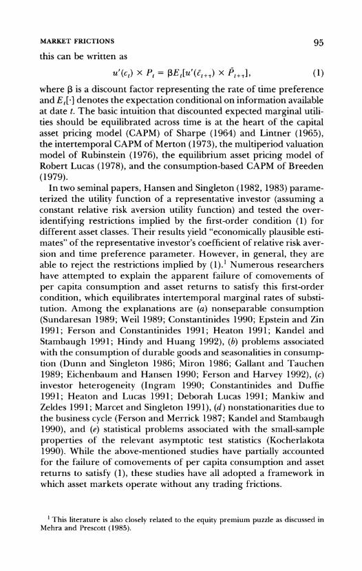
C * Historical IMRS ' 0 - IMRS Volatility Bound .

o ci -, IMRS Bound with Positivity

-o~~FG 1. IR frnter nomre fitos15-0 >h ...rn 957 Confidenceightedr otfloofalatcslnthse

03

NYSE stocks. Monthly fraontie:ly madjuste frealtconsumto of959n90)

rables and services, 16 the implicit consumption deflator, and population data were obtained from the Citibase database.'7 All returns series were deflated using the implicit consumption deflator for nondurables and services. The monthly consumption data are available only since 1959, and hence our results are based on data from the 1959-90 period.

B. Graphical Results

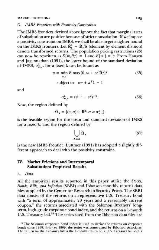
In this subsection, we plot the mean-standard deviation frontier for IMRS implied by returns and compare it to the IMRS computed from historical consumption data. Figure I depicts the failure of the IMRS

minimum maturity of at least 1 month. For a more complete description of the SBBI series, see Ibbotson Associates (1991).

16 As noted in previous studies, the U.S. Commerce Department's X1I seasonal filter does not remove all the seasonal dependencies in the consumption data. For instance, strong monthly seasonals remain. There also appear to be calendar dependencies based on the number of days in the month and the number of Mondays, Tuesdays, etc. in a month.

17 The population series (POPRES) is a first of the month estimate of the total resi- dent population excluding armed forces overseas.


bounds, implied by asset returns in a frictionless world, to satisfy the first-order conditions given by (1). The solid and dashed lines in figure 1 plot the mean and standard deviation frontier of IMRS implied by the returns on a value-weighted portfolio of NYSE stocks, an equally weighted portfolio of the same stock universe, long-term U.S. Treasury bonds, an index of high-grade corporate bonds, and 1-month Treasury bills. In all the figures, the solid line represents the IMRS frontier without the positivity constraint and the dashed line is the corresponding curve with the positivity constraint. The dotted lines surrounding the returns-based IMRS frontiers define the 95 percent confidence interval for the point estimates of the two frontiers. These confidence bounds were computed using Monte Carlo techniques, which assume that the natural logarithm of one plus the return series are multivariate normal."8 An examination of figure 1 reveals that the size of the 95 percent confidence interval is approximately the same for the frontiers with and without the positivity constraint. Hence in figures 2-6, we present a confidence interval only for the frontier that does not impose the positivity constraint since numerically this region is much easier to compute.

Figures 1-6 also plot the time-series sample means and standard deviations of IMRS implied by an average investor with a constant relative risk aversion utility function of the form

U(ct) = - , t a>0. 1-a -t

A time preference discount factor X of .99754 is used for the figures.19 The black diamond symbols represent mean-standard deviation pairs of historical IMRS computed using consumption of nondurables and services for alternative values of ot ranging from zero to 60 in one-unit increments.20 We have restricted the visible region of the graphs, and hence all 61 mean and standard deviation IMRS points will not generally be shown. In all cases, the most southeast point corresponds to ao = 0.

18 The sample skewness and kurtosis statistics suggest that the return series are not lognormally distributed. All the return series have fatter tails than would be expected from a normal distribution. In addition, the equity return series are skewed to the left with evidence of long tails in the positive direction. There is some tendency for fixed income returns to be skewed to the right with long tails in the opposite direction. This evidence of nonnormal distributions may impinge on the small-sample reliability of the confidence intervals. The returns were generated assuming a vector autoregressive system with lags 1-6, 9, and 12. The confidence bounds are based on 3,000 simulations.

19 This corresponds to an annual discount factor of .97. 20 Since we consider the graphs to be primarily diagnostic, we do not present confi-

dence regions for the mean-standard deviation pairs of historical IMRS or formally test whether these point estimates lie outside the confidence regions for the volatility frontiers.

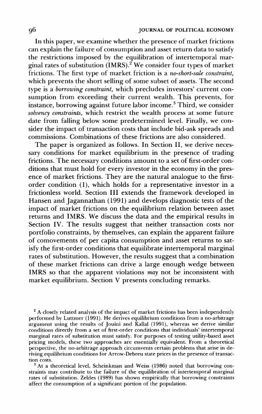
00~ ~ ~ ~~I

C I .0I O CN L * Historical IMRS > - - IMRS Volatility Bound I

to (D _ - IMRS Bound with Positivity 957 Confidence Interval

C-

00

0D 0.974 0.978 0.982 0.986 0.990 0.994 0.998 1.002 1.006 1.010

Mean

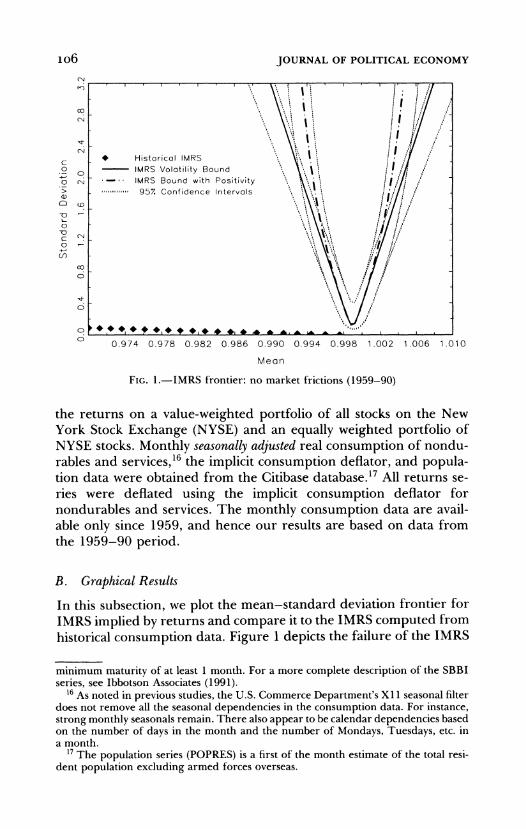
FIG. 2.-LMRS frontier: no short sale of the riskless asset (1959 90)

clJ

c-J

cz co * Historical iMRS >) - IMRS Volatility Bound

CD - MRS Bound with Positivity -o tt:l l.,,,,,,,957. Confidence Interval

FIG 3.J IMSfote:broig osrit15-0

0 ~ ~ ~ ~ ~ ~ ~ 0

0-

0D 0.974 0.978 0.982 0.986 0.990 0.994 0.998 1 002 1 006 1.010

Mean

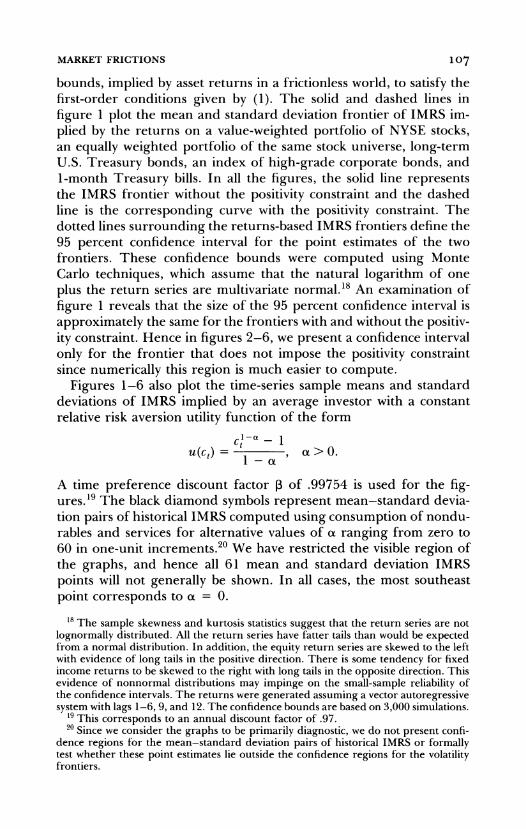
FIG. 3.-LMRS frontier: borrowing constraints (1959 90)

io8

DC

O (N * Historical IMRS > - - IMRS Volatility Bound

C0 u IMRS Bound with Positivity 95% Confidence Interval

CO

CD>

CD ,, Ai,.

o

? 0.974 0.978 0.982 0.986 0.990 0.994 0.998 1.002 1.006 1.010

Mean

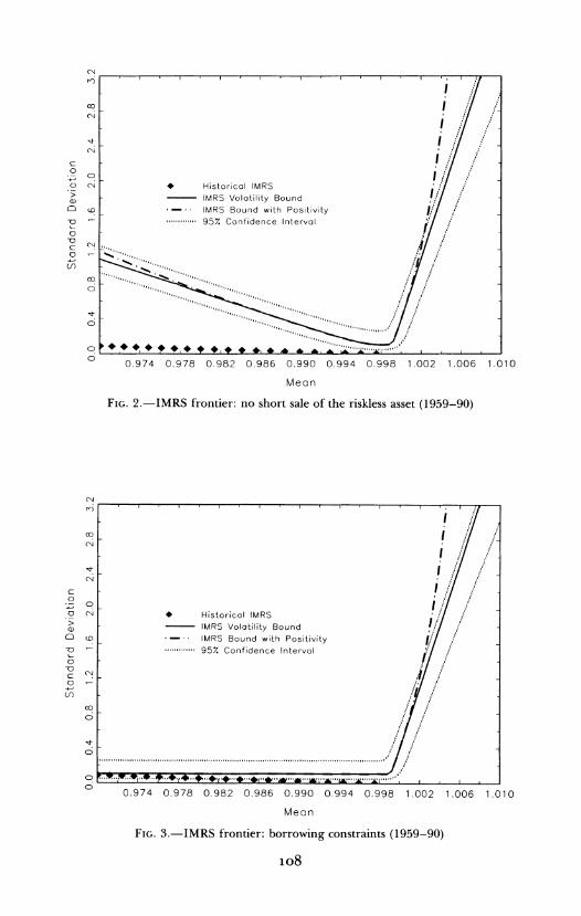
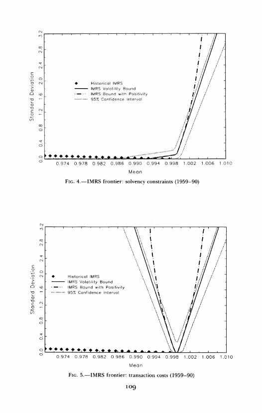
FIG. 4.-IMRS frontier: solvency constraints (1959-90)

toi * Historical IMRS >, IMRS Volatility Bound

t O - IMRS Bound with Positivity ....957. Confidence Intervalp

? 0.974 0.978 0.982 0.986 0,990 0.994 0.998 1.002 1.006 1.010

Mean

FIG. 5. IMRS frontier: transaction costs (1959-90)

log


CN I

C A * Historical IMRS ,

) IMRS Volatility Bound CD IMRS Bound with Positivity

D . 957. Confidence Interval

0 J CD o 1/

CD

0.974 0.978 0.982 0.986 0.990 0.994 0.998 1.002 1.006 1.010

Mean

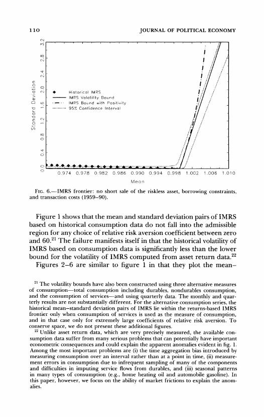
FIG. 6.-IMRS frontier: no short sale of the riskless asset, borrowing constraints, and transaction costs (1959-90).

Figure 1 shows that the mean and standard deviation pairs of IMRS based on historical consumption data do not fall into the admissible region for any choice of relative risk aversion coefficient between zero and 60.21 The failure manifests itself in that the historical volatility of IMRS based on consumption data is significantly less than the lower bound for the volatility of IMRS computed from asset return data.22

Figures 2-6 are similar to figure 1 in that they plot the mean-

21 The volatility bounds have also been constructed using three alternative measures of consumption-total consumption including durables, nondurables consumption, and the consumption of services-and using quarterly data. The monthly and quarterly results are not substantially different. For the alternative consumption series, the historical mean-standard deviation pairs of IMRS lie within the returns-based IMRS frontier only when consumption of services is used as the measure of consumption, and in that case only for extremely large coefficients of relative risk aversion. To conserve space, we do not present these additional figures.

22 Unlike asset return data, which are very precisely measured, the available consumption data suffer from many serious problems that can potentially have important econometric consequences and could explain the apparent anomalies evident in fig. 1. Among the most important problems are (i) the time aggregation bias introduced by measuring consumption over an interval rather than at a point in time, (ii) measure- ment errors in consumption due to infrequent sampling of many of the components and difficulties in imputing service flows from durables, and (iii) seasonal patterns in many types of consumption (e.g., home heating oil and automobile gasoline). In this paper, however, we focus on the ability of market frictions to explain the anomalies.

MARKET FRICTIONS i11

standard deviation pairs of historical IMRS based on consumption data for a range of relative risk aversion coefficients. These figures also contain plots of the IMRS volatility lower bounds, implied by asset returns in the presence of market frictions, for a range of hypo- thetical prices for the real unit discount bond. In each of these figures, the solid curve is the lower bound without the positivity constraint on IMRS and the dashed curve is the lower bound imposing positivity. As noted above, the 95 percent confidence interval is repre- sented by a dotted curve.

Figure 2 plots the IMRS frontier in the presence of a short-sale constraint for the special case in which the riskless asset (Treasury bills) is the sole asset that cannot be shorted. Figure 2 shows that the no-short-sale constraint shifts the admissible IMRS region downward, although not sufficiently downward to explain the IMRS based on consumption data. The relevant first-order conditions in the presence of this constraint are

E[I3Ut?)1) = 1

and

E au (et+1) Rftj 1 Xf 1.

Our diagnostic empirical procedure searches for the Xf that minimizes the volatility of IMRS based on the return data.23 A different value of Xf is found for each possible value of v, the implicit price of a unit discount bond. The volatility-minimizing Xf corresponding to a mean v of .9976 is equal to .9987 in figure 2 and results in a lower bound in the volatility of IMRS of .1003. We focus on this value of v in our discussion in the text since it approximately corresponds to a real riskless rate of 3 percent per year, which would seem to be a reason- able upper bound for riskless real rates if such securities existed. In this figure and for this choice of v, the volatility frontiers with and without the positivity constraint coincide, leading to identical IMRS volatilities and Xis.

The imposition of borrowing constraints results in a more dramatic shift in the IMRS frontier, which is shown in figure 3, although it is still insufficient to be consistent with the low historical volatility of IMRS based on consumption data for coefficients of relative risk aversion that are less than approximately 10. For an implicit price of a

23 The X's for the risky assets, in the presence of only a short-sale constraint, are equal to one.


unit discount bond v equal to .9976, X equal to .9987 for all assets24 minimizes the standard deviation of the portfolio with payoffs vto, which is equal to .1062. The volatility of ex post IMRS based on consumption data in this region, where the real riskless rate is approximately 3 percent per year, is less than one-tenth of the volatility bound based on returns. As above, the volatility frontiers with and without positivity constraints coincide for this choice of v. We present in figure 4 the return-based IMRS frontiers in the presence of solvency constraints. The primary difference between solvency and borrowing constraints is that solvency constraints place a restriction on future wealth, for example, WH1, ' L,,,. Hence current financial wealth can in principle be negative (given positive future labor income), whereas borrowing constraints place a restriction on current financial wealth (i.e., ct - Wt.). For implementation purposes, the primary distinction is that in the presence of borrowing constraints the X for all risky assets will be the same and less than or equal to one, whereas they need not be equal under solvency constraints. Relax- ation of the equality restriction results in a smaller lower bound on the volatility of IMRS in the presence of solvency constraints than that depicted in figure 3 in the presence of borrowing constraints. For values of the coefficient of relative risk aversion larger than approximately two, the historical IMRS using consumption data now lie inside the returns-based IMRS frontier. The associated X's for the value- and equally weighted stock indices, Treasury bonds, corporate bonds, and Treasury bills are, respectively, .9993, 1.000, .9984, .9987, and .9986 when positivity is not imposed and .9999, 1.000, 1.000, .9997, and .9997 when positivity is imposed. The lower bound on the volatility of IMRS corresponding to v = .9976 is .0811 for both frontiers.

Figure 5 examines the impact of transaction costs. We assume the following transaction costs: 0.75 percent for the value-weighted portfolio, 1.5 percent for the equally weighted portfolio, 0.015 percent for Treasury bills, 0.03 percent for Treasury bonds, and 0.5 percent for corporate bonds.25 As is readily apparent, the introduction of transaction costs by itself does little to explain the disparity between historical IMRS based on consumption data and the returns-based IMRS frontier plotted in figure 1.

24 For this case, the A's for all the assets are constrained to be equal although they may differ from one.

25 All transaction cost figures are presented as order of magnitude estimates. They are estimates of current costs. These numbers should thus serve as lower bounds to the costs incurred by traders in earlier years. Some investors, however, who are forced to purchase or liquidate assets may effectively face zero marginal transaction costs. The equity numbers were obtained from the database of the Institute for the Study of Security Markets for the month of September 1987.


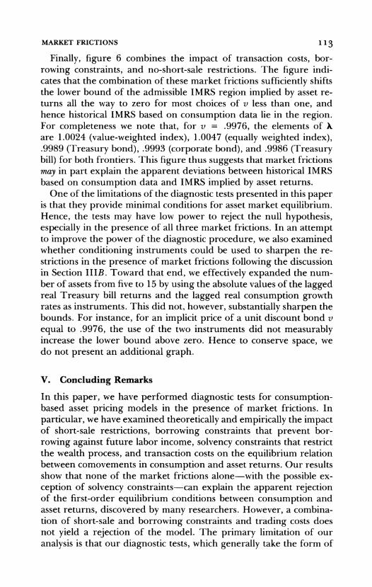
Finally, figure 6 combines the impact of transaction costs, borrowing constraints, and no-short-sale restrictions. The figure indicates that the combination of these market frictions sufficiently shifts the lower bound of the admissible IMRS region implied by asset returns all the way to zero for most choices of v less than one, and hence historical IMRS based on consumption data lie in the region. For completeness we note that, for v = .9976, the elements of X are 1.0024 (value-weighted index), 1.0047 (equally weighted index), .9989 (Treasury bond), .9993 (corporate bond), and .9986 (Treasury bill) for both frontiers. This figure thus suggests that market frictions may in part explain the apparent deviations between historical IMRS based on consumption data and IMRS implied by asset returns.

One of the limitations of the diagnostic tests presented in this paper is that they provide minimal conditions for asset market equilibrium. Hence, the tests may have low power to reject the null hypothesis, especially in the presence of all three market frictions. In an attempt to improve the power of the diagnostic procedure, we also examined whether conditioning instruments could be used to sharpen the restrictions in the presence of market frictions following the discussion in Section IIIB. Toward that end, we effectively expanded the number of assets from five to 15 by using the absolute values of the lagged real Treasury bill returns and the lagged real consumption growth rates as instruments. This did not, however, substantially sharpen the bounds. For instance, for an implicit price of a unit discount bond v equal to .9976, the use of the two instruments did not measurably increase the lower bound above zero. Hence to conserve space, we do not present an additional graph.

V. Concluding Remarks

In this paper, we have performed diagnostic tests for consumption- based asset pricing models in the presence of market frictions. In particular, we have examined theoretically and empirically the impact of short-sale restrictions, borrowing constraints that prevent borrowing against future labor income, solvency constraints that restrict the wealth process, and transaction costs on the equilibrium relation between comovements in consumption and asset returns. Our results show that none of the market frictions alone-with the possible ex- ception of solvency constraints-can explain the apparent rejection of the first-order equilibrium conditions between consumption and asset returns, discovered by many researchers. However, a combination of short-sale and borrowing constraints and trading costs does not yield a rejection of the model. The primary limitation of our analysis is that our diagnostic tests, which generally take the form of


inequality restrictions, are likely to be significantly weaker than the standard tests of equality restrictions.

Appendix

In order to avoid technical problems that can potentially arise for utility functions that have infinite marginal utility at a zero consumption level, we make the following two assumptions: the consumption plan at the optimum is strictly positive and bounded away from zero, and all the returns Rjt+ have compact support.

Proof of Equilibrium Conditions in the Presence of Transaction Costs

Consider shifting A > 0 dollars from current consumption to next period's consumption through investing in asset j. This results in a net investment of AI/(1 + pj) dollars in asset j. The additional consumption generated by this strategy for the next period is [(1 - pj)/( + pj)] AR;,t+ l. Since any deviation from the optimal consumption plan (in the presence of transaction costs) diminishes expected utility, we get

-u'(ct) + PEt u'(et+l)( 12 p t SO,

and hence

Lt u'(e4+1) -1,

1 + pi uE(ct) R1,t+1j 1 -

Similarly, shifting A < 0 dollars from current consumption to consumption next period yields

UE(cV) t+l 1 + Pj

Q.E.D.

Proof of Equilibrium Conditions in the Presence of Short-Sale Restrictions on the Riskless Asset, Transaction Costs, and Borrowing Constraints

As in the previous proof, consider shifting A > 0 dollars from current consumption to next period's consumption through investing in asset j or the riskless asset. Using the same argument, we obtain (16) and (17). Note that these two inequality conditions are one-sided, since we may not be able to shift A < 0 dollars from current consumption to next period's consumption because of the borrowing constraints.

Next, consider shifting A > 0 dollars from assetj to asset i. This yields the first inequality in (18). Again, consider shifting A > 0 dollars from asset i to assetj. This yields the second inequality in (18).


Finally, consider shifting A > 0 dollars from asset i to the riskless asset. This yields (19). Note that (19) is one-sided because of the short-sale constraints for the riskless asset. Q.E.D.

References

Breeden, Douglas T. "An Intertemporal Asset Pricing Model with Stochastic Consumption and Investment Opportunities."J. Financial Econ. 7 (Septem- ber 1979): 265-96.

Cecchetti, Stephen G.; Lam, Pok-sang; and Mark, Nelson C. "Testing Volatil- ity Restrictions on Intertemporal Marginal Rates of Substitution Implied by Euler Equations and Asset Returns." Manuscript. Columbus: Ohio State Univ., Dept. Econ., 1992.

Cochrane, John H., and Hansen, Lars Peter. "Asset Pricing Lessons for Mac- roeconomics." Manuscript. Chicago: Univ. Chicago, Dept. Econ., 1992.

Constantinides, George M. "Habit Formation: A Resolution of the Equity Premium Puzzle." J.P.E. 98 (June 1990): 519-43.

Constantinides, George M., and Duffie, Darrell. "Asset Pricing with Hetero- geneous Consumers: Good News and Bad News." Manuscript. Chicago: Univ. Chicago, Grad. School Bus., 1991.

Dunn, Kenneth B., and Singleton, Kenneth J. "Modeling the Term Structure of Interest Rates under Nonseparable Utility and Durability of Goods."J. Financial Econ. 17 (September 1986): 27-55.

Eichenbaum, Martin S., and Hansen, Lars Peter. "Estimating Models with Intertemporal Substitution Using Aggregate Time Series Data."J. Bus. and Econ. States. 8 (January 1990): 53-69.

Epstein, Larry G., and Zin, Stanley E. "Substitution, Risk Aversion, and the Temporal Behavior of Consumption and Asset Returns: An Empirical Analysis." J.P.E. 99 (April 1991): 263-86.

Ferson, Wayne E., and Constantinides, George M. "Habit Persistence and Durability in Aggregate Consumption: Empirical Tests."J. Financial Econ. 29 (October 1991): 199-240.

Ferson, Wayne E., and Harvey, Campbell R. "Seasonality and Consumption- Based Asset Pricing."J. Finance 47 (June 1992): 511-52.

Ferson, Wayne E., and Merrick, John J., Jr. "Non-stationarity and Stage-of- the-Business-Cycle Effects in Consumption-Based Asset Pricing Relations." J. Financial Econ. 18 (March 1987): 127-46.

Gallant, A. Ronald, and Tauchen, George. "Seminonparametric Estimation of Conditionally Constrained Heterogeneous Processes: Asset Pricing Ap- plications." Econometrica 57 (September 1989): 1091-1120.

Hansen, Lars Peter; Heaton, John; and Jagannathan, Ravi. "Econometric Evaluation of Intertemporal Asset Pricing Models Using Volatility Bounds." Manuscript. Chicago: Univ. Chicago, Dept. Econ.; Cambridge, Mass.: NBER, 1992.

Hansen, Lars Peter, and Jagannathan, Ravi. "Implications of Security Market Data for Models of Dynamic Economies." J.P.E. 99 (April 1991): 225-62.

Hansen, Lars Peter, and Singleton, Kenneth J. "Generalized Instrumental Variables Estimation of Nonlinear Rational Expectations Models." Econo- metrica 50 (September 1982): 1269-86.

"Stochastic Consumption, Risk Aversion, and the Temporal Behavior of Asset Returns." J.P.E. 91 (April 1983): 249-65.


Heaton, John. "An Empirical Examination of Asset Pricing with Temporally Dependent Preference Specifications." Manuscript. Cambridge: Massachu- setts Inst. Tech., Sloan School Management, 1991.

Heaton, John, and Lucas, Deborah J. "Evaluating the Effects of Incomplete Markets on Risk Sharing and Asset Pricing." Manuscript. Cambridge: Mas- sachusetts Inst. Tech., Dept. Econ., 1991.

Hindy, Ayman, and Huang, Chi-fu. "Intertemporal Preferences for Uncer- tain Consumption: A Continuous Time Approach." Econometrica 60 (July 1992): 781-801.

Ibbotson Associates. Stocks, Bonds, Bills, and Inflation: Market Results for 1926-90. New Haven, Conn.: Ibbotson Assoc., 1991.

Ingram, Beth Fisher. "Equilibrium Modeling of Asset Prices: Rationality ver- sus Rules of Thumb."J. Bus. and Econ. Statis. 8 (January 1990): 115-25.

Jouini, E., and Kallal, Hedi. "Martingales, Arbitrage and Equilibrium in Secu- rities Markets with Transaction Costs." Manuscript. Chicago: Univ. Chi- cago, Dept. Econ., 1991.

Kandel, Shmuel, and Stambaugh, Robert F. "Expectations and Volatility of Consumption and Asset Returns." Rev. Financial Studies 3, no. 2 (1990): 207-32.

. "Asset Returns and Intertemporal Preferences."J. Monetary Econ. 27 (February 1991): 39-71.

Kocherlakota, Narayana R. "On Tests of Representative Consumer Asset Pricing Models." J. Monetary Econ. 26 (October 1990): 285-304.

Lintner, John. "The Valuation of Risk Assets and the Selection of Risky Investments in Stock Portfolios and Capital Budgets." Rev. Econ. and Statis. 47 (February 1965): 13-37.

Lucas, Deborah J. "Asset Pricing with Undiversifiable Income Risk and Short Sales Constraints: Deepening the Equity Premium Puzzle." Manuscript. Evanston, Ill.: Northwestern Univ., Kellogg Grad. School Management, 1991.

Lucas, Robert E., Jr. "Asset Prices in an Exchange Economy." Econometrica 46 (November 1978): 1429-45.

Luttmer, Erzo G. "Asset Pricing in Economies with Frictions." Manuscript. Chicago: Univ. Chicago, Dept. Econ., 1991.

Marcet, Albert, and Singleton, Kenneth J. "Optimal Consumption-Savings Decisions and Equilibrium Asset Prices in a Model with Heterogeneous Agents Subject to Portfolio Constraints." Manuscript. Stanford, Calif.: Stanford Univ., Grad. School Bus., 1991.

Mankiw, N. Gregory, and Zeldes, Stephen P. "The Consumption of Stock- holders and Nonstockholders."J. Financial Econ. 29 (March 1991): 97-112.

Mehra, Rajnish, and Prescott, Edward C. "The Equity Premium: A Puzzle." J. Monetary Econ. 15 (March 1985): 145-61.

Merton, Robert C. "An Intertemporal Capital Asset Pricing Model." Econo- metrica 41 (September 1973): 867-87.

Miron, Jeffrey A. "Seasonal Fluctuations and the Life Cycle-Permanent In- come Model of Consumpion."J.P.E. 94 (December 1986): 1258-79.

Rubinstein, Mark. "The Valuation of Uncertain Income Streams and the Pricing of Options." Bellj. Econ. 7 (Autumn 1976): 407-25.

Scheinkman, Jose A., and Weiss, Laurence. "Borrowing Constraints and Ag- gregate Economic Activity." Econometrica 54 (January 1986): 23-45.

Sharpe, William F. "Capital Asset Prices: A Theory of Market Equilibrium under Conditions of Risk."J. Finance 19 (September 1964): 425-42.


Sundaresan, Suresh M. "Intertemporally Dependent Preferences and the Volatility of Consumption and Wealth." Rev. Financial Studies 2, no. 1 (1989): 73-89.

Weil, Philippe. "The Equity Premium Puzzle and the Risk-Free Rate Puzzle." J. Monetary Econ. 24 (November 1989): 401-21.

Zeldes, Stephen P. "Consumption and Liquidity Constraints: An Empirical Investigation."J.P.E. 97 (April 1989): 305-46.

Documents

Market Frictions and Consumption-Based Asset Pricing