A measurement of large-scale peculiar velocities of clusters of

galaxies: technical details

A. Kashlinsky1,5, F. Atrio-Barandela2, D. Kocevski3, H. Ebeling4

ABSTRACT

This paper presents detailed analysis of large-scale peculiar motions derived

from a sample of ∼ 700 X-ray clusters and cosmic microwave background (CM-

B) data obtained with WMAP. We use the kinematic Sunyaev-Zeldovich (KSZ)

effect combining it into a cumulative statistic which preserves the bulk motion

component with the noise integrated down. Such statistic is the dipole of CMB

temperature fluctuations evaluated over the pixels of the cluster catalog (Kash-

linsky & Atrio-Barandela 2000). To remove the cosmological CMB fluctuations

the maps are Wiener-filtered in each of the eight WMAP channels (Q, V, W)

which have negligible foreground component. Our findings are as follows: The

thermal SZ (TSZ) component of the clusters is described well by the Navarro-

Frenk-White profile expected if the hot gas traces the dark matter in the cluster

potential wells. Such gas has X-ray temperature decreasing rapidly towards the

cluster outskirts, which we demonstrate results in the decrease of the TSZ com-

ponent as the aperture is increased to encompass the cluster outskirts. We then

detect a statistically significant dipole in the CMB pixels at cluster positions.

Arising exclusively at the cluster pixels this dipole cannot originate from the

foreground or instrument noise emissions and must be produced by the CM-

B photons which interacted with the hot intracluster gas via the SZ effect. The

dipole remains as the monopole component, due to the TSZ effect, vanishes with-

in the small statistical noise out to the maximal aperture where we still detect the

TSZ component. We demonstrate with simulations that the mask and cross-talk

effects are small for our catalog and contribute negligibly to the measurements.

1SSAI and Observational Cosmology Laboratory, Code 665, Goddard Space Flight Center, Greenbelt MD20771

2Fisica Teorica, University of Salamanca, 37008 Salamanca, Spain

3Department of Physics, University of California at Davis, 1 Shields Avenue, Davis, CA 95616

4Institute for Astronomy, University of Hawaii, 2680 Woodlawn Drive, Honolulu, HI 96822

5e–mail: alexander.kashlinsky@nasa.gov

– 2 –

The measured dipole thus arises from the KSZ effect produced by the coherent

large scale bulk flow motion. The cosmological implications of the measurements

are discussed by us in Kashlinsky et al (2008).

Subject headings: cosmology: observations - cosmic microwave background - early

Universe - large-scale structure of universe - methods: numerical - methods:

statistical

1. Introduction

In the popular gravitational instability picture for growth of the large scale struc-

ture in the Universe, peculiar velocities on large cosmological scales probe directly the pe-

culiar gravitational potential and provide important information on the underlying mass

distribution in the Universe [e.g. see review by Kashlinsky & Jones 1991]. Previous at-

tempts to measure the peculiar flows in the local Universe mostly used empirically estab-

lished (but not well understood theoretically) galaxy distance indicators. While very im-

portant, such methods are subject to many systematic uncertainties [e.g. see reviews by

(Strauss & Willick 1995; Willick 2000)] and lead to widely different results.

Early measurements by (Rubin et al 1976) indicated large peculiar flows of ∼700 k-

m/sec. A major advance was made using the “Fundamental Plane” (FP) relation for elliptical

galaxies (Dressler et al 1987; Djorgovski & Davis 1987) with the implication that elliptical

galaxies within ∼ 60h−1Mpc were streaming at ∼ 600 km/sec with respect to the rest frame

defined by the cosmic microwave background (CMB) (Lynden-Bell et al 1988). Mathewson

et al (1992) used the Tully-Fisher (TF) relation for a large sample of spiral galaxies suggest-

ing that the flow of amplitude 600 km/sec does not converge until scales much larger than

∼ 60h−1 Mpc. This finding was in agreement with a later analysis by (Willick 1999). Em-

ploying brightest cluster galaxies as distance indicators (Lauer & Postman 1994) measured

a bulk flow of ∼700 km/sec for a sample 119 rich clusters of galaxies on scale of ∼150h−1Mpc

suggesting significantly larger amount of power than expected in the concordance ΛCDM

model. However, a re-analysis of these data (Hudson & Ebeling 1997) taking into account

the correlation between the luminosities of brightest-cluster galaxies and that of their host

cluster found a greatly reduced bulk flow. Using the FP relation for early type galaxies

in 56 clusters (Hudson et al 1999) find a bulk flow of a similarly large amplitude of ∼ 630

km/sec to (Lauer & Postman 1994) on a comparable scale, but in a different direction. On

the other hand, a sample of ∼ 104 SNIa shows no evidence of significant bulk flows out to

∼ 100h−1 Mpc (Riess et al 1997) and similar conclusion is reached with the TF based survey

of spiral galaxies by (Courteau et al 2000). The directions associated with each bulk-flow

– 3 –

measurement are equally discrepant.

The current situation with measurements based on the various distance indicators is

confusing and it is important to find alternative ways to measure the large scale peculiar

flows. One way to achieve this is via the kinematic component of the Sunyaev Zeldovich

(SZ) effect produced on the CMB photons from the hot X-ray emitting gas in clusters of

galaxies ([see review by (Birkinshaw 1999)]. The kinematic SZ (KSZ) effect is independent

of redshift and measures the line-of-sight peculiar velocity of a cluster in its own frame

of reference. For each individual cluster the KSZ temperature distortion will be small and

difficult to measure. Attempts at measuring the peculiar velocities of individual clusters from

the KSZ effect using the current generation of instruments lead to uncertainties of >∼1000

km/sec per cluster [see review by (Carlstrom et al 2002)]. On the other hand, as proposed

by (Kashlinsky & Atrio-Barandela 2000) (hereafter KA-B) for many clusters moving at a

coherent bulk flow one can construct a measurable quantity using data on CMB temperature

anisotropies which will be dominated by the bulk flow KSZ component, whereas the various

other contributions will integrate down. This quantity, the dipole of the cumulative CMB

temperature field evaluated at cluster positions, is used in this investigation on the 3-year

WMAP data in conjunction with a large sample of X-ray clusters of galaxies to set the

strongest to-date limits on bulk flows out to scales ∼ 300h−1Mpc.

In the accompanying Letter (Kashlinsky et al 2008) we summed the results and their

cosmological implications. These are obtained using the KA-B method applied to 3-year

WMAP CMB data and the largest all-sky X-ray cluster catalog to date. This paper provides

the details relevant for the measurement and is structured as follows: Sec 2 summarizes the

KA-B method and the steps leading to the measurement. Sec. 3 describes the cluster

X-ray catalog used in this study and Sec. 4 outlines the CMB data processing. Sec. 5

discusses the methods to estimate the errors followed by Sec 6 with the results on the dipole

measurement. Sec. 7 shows why the measured dipole arises from the KSZ component due

to the cluster motion and Sec. 8 dicusses the translation of the measured dipole in µK into

velocity in km/sec and its uncertainty. Future prospects foreseeable at this time to improve

this measurement are discussed in Sec. 9. We summarize our results in Sec. 10.

2. KA-B method and steps to the measurement

If a cluster at angular position y has the line-of-sight velocity v with respect to the

CMB, the SZ CMB fluctuation at frequency ν at this position will be δν(y) = δTSZ(y)G(ν)+

δKSZ(y)H(ν), with δTSZ=τTX/Te,ann and δKSZ=τv/c. Here G(ν) −1.85 to −1.35 and

H(ν) 1 over the range of frequencies probed by the WMAP data, τ is the projected optical

– 4 –

depth due to Compton scattering, TX is the cluster electron temperature and kBTe,ann=511

KeV. If averaged over many isotropically distributed clusters moving at a significant bulk

flow with respect to the CMB, the kinematic term may dominate enabling a measurement

of Vbulk. Thus KA-B suggested measuring the dipole component of δν(y). Below we use

the notation for C1,kin normalized so that a coherent motion at velocity Vbulk would lead to

C1,kin = T 2CMB〈τ〉2V 2

bulk/c2, where TCMB = 2.725K is the present-day CMB temperature. For

reference,√

C1,kin 1(〈τ〉/10−3)(Vbulk/100km/sec) µK. When computed from the total of

Ncl positions the dipole also will have positive contributions from 1) the instrument noise, 2)

the thermal SZ (TSZ) component, 3) the cosmological CMB fluctuation component arising

from the last-scattering surface, and 4) the various foreground components at the WMAP

frequency range. The latter contribution can be significant at the two lowest frequency

WMAP channels (K & Ka) and, hence, we restrict this analysis to the WMAP Channels Q,

V & W which have negligible foreground contributions.

For Ncl 1 the dipole of the observed δν becomes:

a1m aKSZ1m + aTSZ

1m + aCMB1m +

σnoise√Ncl

(1)

Here aCMB1m is the residual dipole produced at the cluster pixels by the primordial CMB

anisotropies. The amplitude of the dipole power is C1 =∑m=1

m=−1 |a1m|2.

Additional contributions to eq. 1 come from non-linear evolution/collapse of clusters

(Rees & Sciama 1968), gravitational lensing by clusters (Kashlinsky 1988), unresolved strong

radio sources (present, for instance, in WMAP 5 year data, Nolta et al 2008) and the Inte-

grated Sachs-Wolfe effect from the cluster pixels. All these effects have a dipole signal only

when clusters are inhomogenously distributed on the sky and is in turn bounded from above

by the amplitude of the monopole. The magnitude of these contributions is at most ∼ 10µK2

in power (see Aghanin, Majumdar & Silk 2008 for a review on secondary anisotropies) a fac-

tor of 10 smaller than the Thermal Sunyaev-Zeldovich monopole amplitude. Furthermore, as

we discuss below, we find a dipole signal when the monopole vanishes, so our measurements

can not be significantly affected by all these effects.

In the following sections we detail out the process that enabled us to isolate the KSZ

term in eq. 1. The steps leading to this measurement were:

• An all-sky catalog of X-ray selected galaxy clusters was constructed using available

X-ray data extending to z 0.3.

• The cosmological CMB component was removed from the WMAP data using the

Wiener filter with the best-fit cosmological model.

• The Wiener filter is constructed (and is different) for each DA channel because the

– 5 –

beam and the noise levels are different. This then prevents inconsistencies and systematic

errors that could have been generated if a common filter was applied to the eight channels

of different noise and resolution.

• The filtered CMB maps were used to compute the dipole component at the cluster

positions simultaneously as the TSZ monopole vanishes because of the X-ray temperature

decrease with radius (Atrio-Barandela et al 2008 and below).

• Simulations showed that the measured dipole arises from the cluster pixels at a high

confidence level. Since the TSZ component from the clusters vanishes, only a contribution

from the KSZ component, due to large-scale bulk motion of the cluster sample, remains.

The following sections present the technical details related to this analysis.

3. X-ray data and catalogue

The creation of the all-sky cluster catalogue used here from three independent X-ray

selected cluster samples is described in detail by Kocevski & Ebeling (2006); for clarity we

briefly reiterate the procedure in the following.

The REFLEX catalog consists of 447 clusters with X-ray fluxes greater than 3 × 10−12

erg cm−2 s−1 in the [0.1–2.4] KeV band. The survey is limited to declinations of δ < 2.5,

redshifts of z ≤ 0.3 and Galactic latitudes away from the Galactic plane (|b| > 20). The

eBCS catalog comprises 290 clusters in the Northern hemisphere with X-ray fluxes greater

than 3 × 10−12 erg cm−2 s−1 [0.1–2.4] KeV at Galactic latitude |b| < 20. The sample

is limited to declinations of δ > 0 and redshifts of z ≤ 0.3 and, like REFLEX, the survey

avoids the Galactic plane (|b| > 20). The CIZA sample is the product of the first systematic

search for X-ray luminous clusters behind the plane of the Galaxy. The sample contains 165

clusters with X-ray fluxes greater than 3 × 10−12 erg cm−2 s−1 [0.1–2.4] KeV and redshifts

of z ≤ 0.3.

To obtain a single homogeneous sample the physical properties of all clusters were

recalculated in a consistent manner using publicly available RASS data. Cluster positions

were redetermined from the centroid of each system’s X-ray emission and point sources

within the detection aperture are removed. Total X-ray count rates within an aperture of

1.5 h−150 Mpc radius were calculated taking into account the local RASS exposure time and

background, and converted into unabsorbed X-ray fluxes in the ROSAT broad band [0.1–2.4]

KeV. Total rest-frame luminosities were determined from the fluxes using the cosmological

luminosity distance and a temperature-dependent K -correction. Finally clusters whose X-

– 6 –

ray emission appeared to be dominated by a point source were removed and a flux cut was

applied at 3 × 10−12 erg cm−2 s−1, leaving 349 REFLEX, 268 eBCS, and 165 CIZA clusters

at z ≤ 0.3. The resulting sample is the largest homogeneous, all-sky, X-ray selected cluster

catalog compiled to date, containing 782 clusters over the entire sky. Of these, 468 fall

within z <= 0.1. Further details concerning the statistical properties of the catalog, including

its completeness, can be found in Kocevski & Ebeling (2006).

Our analysis requires knowledge of several parameters describing the properties of the

intra-cluster gas. We determine the X-ray extent of each cluster directly from the RASS

imaging data using a growth-curve analysis. The cumulative profile of the net count rate is

constructed for each system by measuring the counts in successively larger circular apertures

centered on the X-ray emission and subtracting an appropriately scaled X-ray background.

The latter is determined in an annulus from 2 to 3 h−150 Mpc around the cluster centroid.

The extent of each system is then defined as the radius at which the increase in the source

signal is less than the 1σ Poissonian noise of the net count rate. This is essentially the

distance from the cluster center at which the X-ray emission is no longer detectable with

any statistically significance.

– 7 –

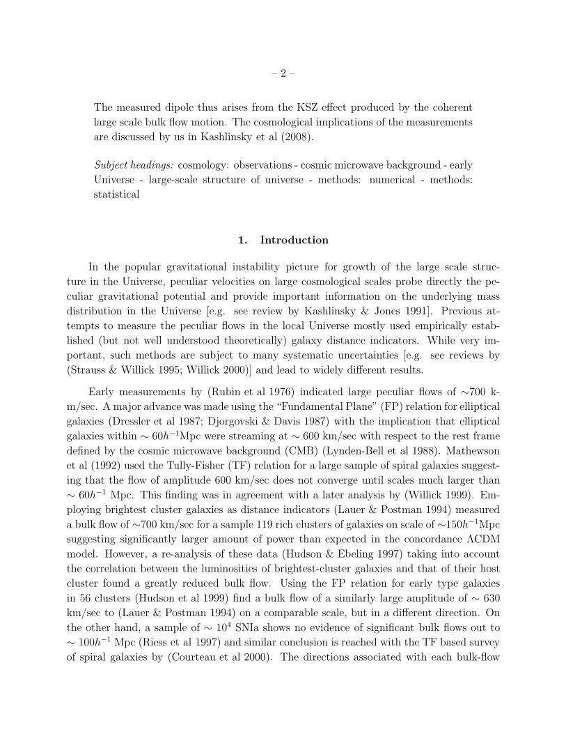
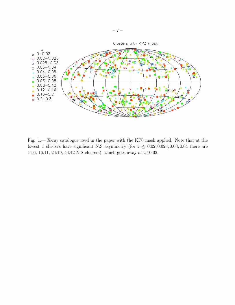
Fig. 1.— X-ray catalogue used in the paper with the KP0 mask applied. Note that at the

lowest z clusters have significant N:S asymmetry (for z ≤ 0.02, 0.025, 0.03, 0.04 there are

11:6, 16:11, 24:19, 44:42 N:S clusters), which goes away at z >∼0.03.

– 8 –

Unabsorbed cluster fluxes were determined from our recalculated count rates by folding

the ROSAT instrument response against the predicted X-ray emission from a Raymond-

Smith (Raymond & Smith 1977) thermal plasma spectrum with 0.3 solar metallicity and

by taking into account Galactic absorption in the direction of the source. The temperature

used in the spectral model is determined iteratively using the cluster redshift, a first-order

approximation on the cluster luminosity using kBTX = 4 KeV and the LX − TX relation

of White et al (1997). Total rest-frame [0.1 − 2.4] KeV band cluster luminosities were

subsequently determined from our recalculated fluxes using the standard conversion with

the cosmological luminosity distance and a temperature dependent K-correction.

To obtain an analytic parametrization of the spatial profile of the X-ray emitting gas

and, ultimately, the central electron density we fit a β model (Cavaliere & Fusco-Femiano

1976) convolved with the RASS point-spread function to the RASS data for each cluster

in our sample: S(r) = S0 [1 + (r/rc)2]

−3β+1/2where S(r) is the projected surface-brightness

distribution and S0, rc, and β are the central surface brightness, the core radius, and the β

parameter characterizing the profile at large radii. Using the results from this model fit to

determine the gas-density profile assumes the gas to be isothermal and spherically symmetric.

In practice, additional uncertainties are introduced by the correlation between rc and β which

makes the results for both parameters sensitive to the choice of radius over which the model

is fit, and the fact that for all but the most nearby clusters the angular resolution of the

RASS allows only a very poor sampling of the surface-brightness profile (at z > 0.2 the

X-ray signal from a typical cluster is only detected in perhaps a dozen RASS image pixels).

In recognition of these limitations, we hold β fixed at the canonical value of 2/3 and only

allow rc to vary (Jones & Forman 1984). As a consistency check, we also calculate rc values

from each cluster’s X-ray luminosity using the rc ∝ L1/3.6X empirical relationship determined

by Reiprich & Bohringer (1999). Our best-fit values for rc are reassuringly robust in the

sense that we find broad agreement with the empirically derived values.

Our best-fit parameters, the cluster luminosity and electron temperature, are used to

determine central electron densities for each cluster using Equation 6 of Henry & Henriksen

(1986) with the temperature of the ICM being estimated from the LX − TX relationship of

White, Jones, & Forman (1997). The electron densities are in turn used to translate the

CMB dipole in µK into an amplitude in km/sec as described below. We also calculated

electron densities using our empirically derived cluster parameters and find good agreement

between the resulting dipole amplitude and the amplitude obtained using our best-fit values.

– 9 –

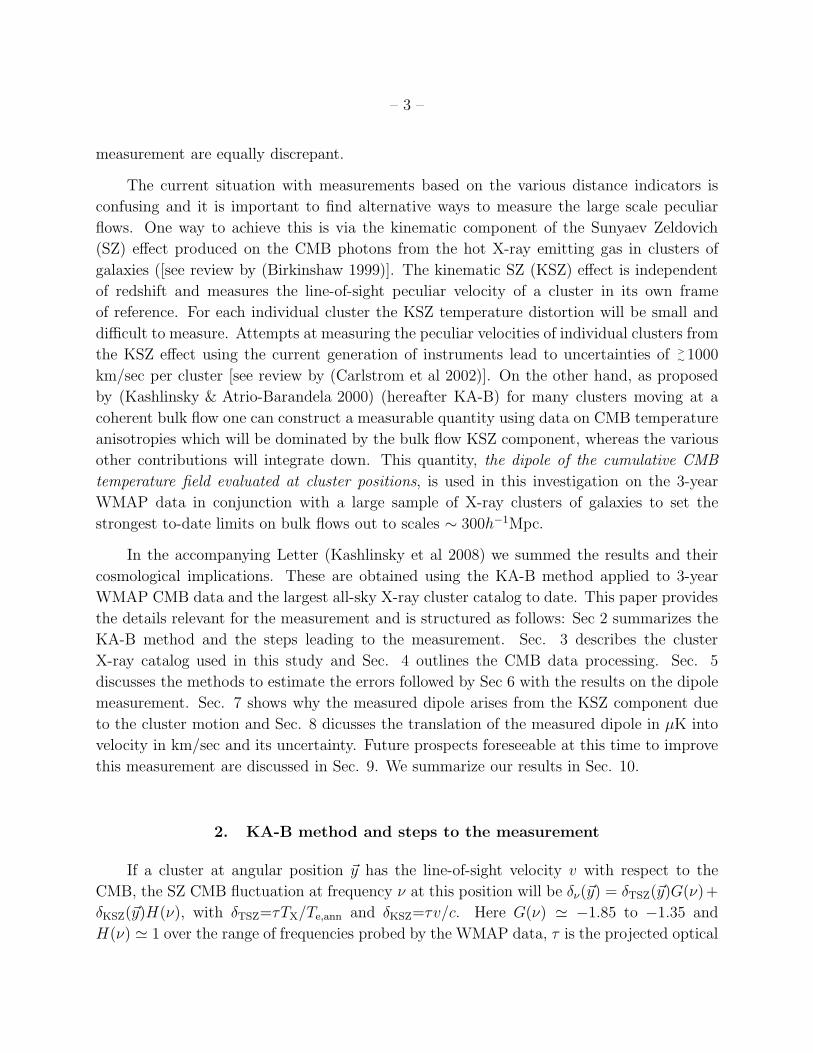
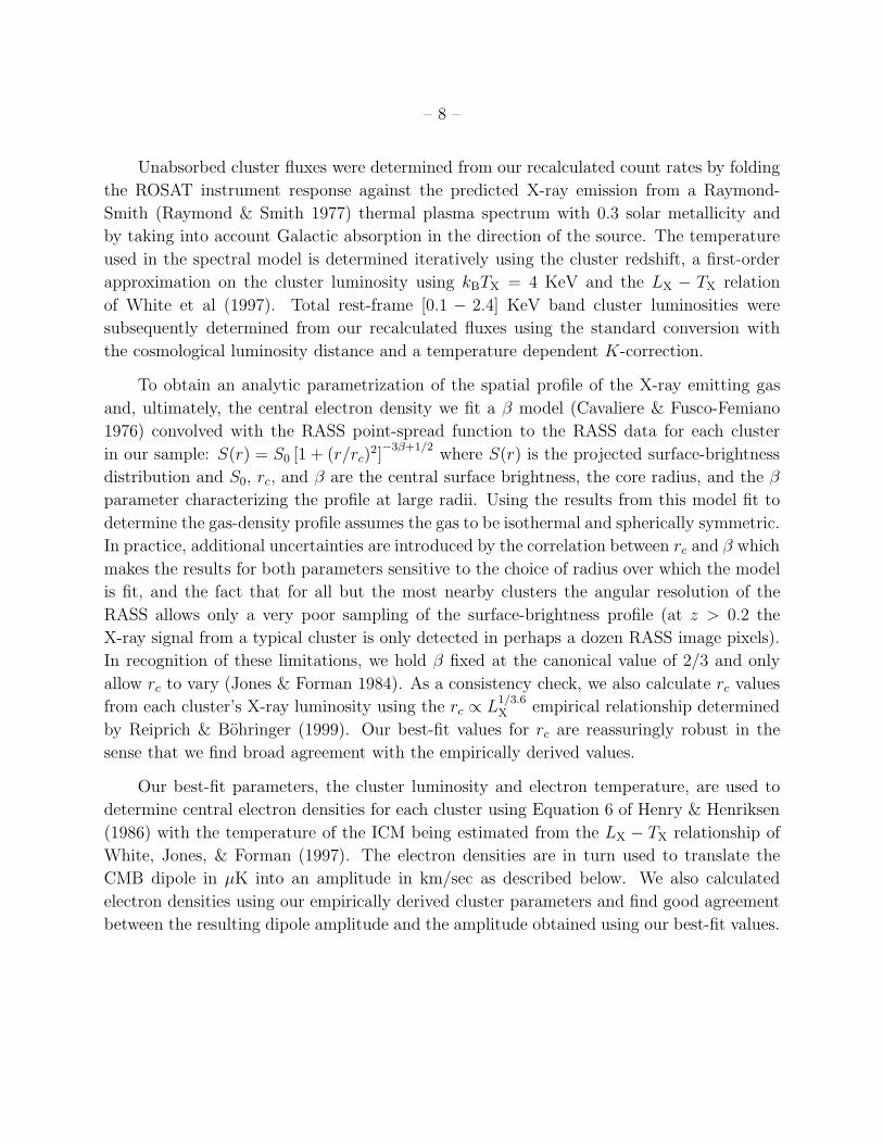
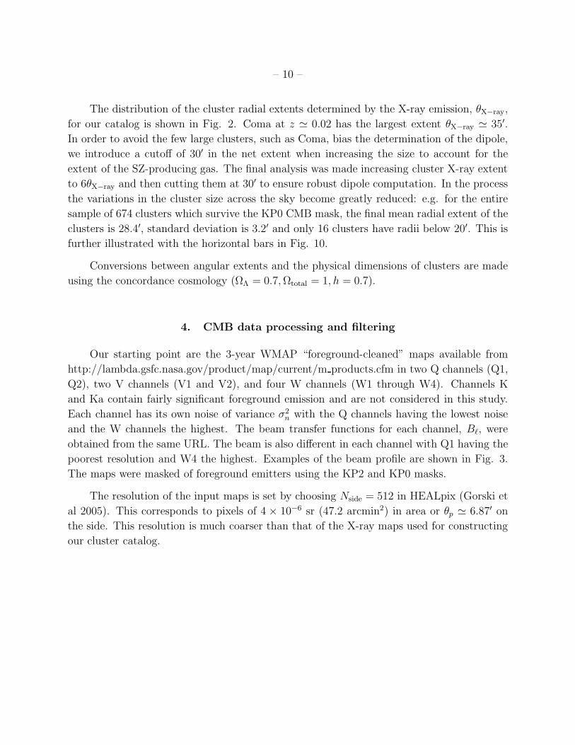
Fig. 2.— Distribution of cluster X-ray extent in various z-bins using the KP0 maps. Coma

is the only cluster with X-ray radial extent larger than 0.5 deg.

– 10 –

The distribution of the cluster radial extents determined by the X-ray emission, θX−ray,

for our catalog is shown in Fig. 2. Coma at z 0.02 has the largest extent θX−ray 35′.

In order to avoid the few large clusters, such as Coma, bias the determination of the dipole,

we introduce a cutoff of 30′ in the net extent when increasing the size to account for the

extent of the SZ-producing gas. The final analysis was made increasing cluster X-ray extent

to 6θX−ray and then cutting them at 30′ to ensure robust dipole computation. In the process

the variations in the cluster size across the sky become greatly reduced: e.g. for the entire

sample of 674 clusters which survive the KP0 CMB mask, the final mean radial extent of the

clusters is 28.4′, standard deviation is 3.2′ and only 16 clusters have radii below 20′. This is

further illustrated with the horizontal bars in Fig. 10.

Conversions between angular extents and the physical dimensions of clusters are made

using the concordance cosmology (ΩΛ = 0.7, Ωtotal = 1, h = 0.7).

4. CMB data processing and filtering

Our starting point are the 3-year WMAP “foreground-cleaned” maps available from

http://lambda.gsfc.nasa.gov/product/map/current/m products.cfm in two Q channels (Q1,

Q2), two V channels (V1 and V2), and four W channels (W1 through W4). Channels K

and Ka contain fairly significant foreground emission and are not considered in this study.

Each channel has its own noise of variance σ2n with the Q channels having the lowest noise

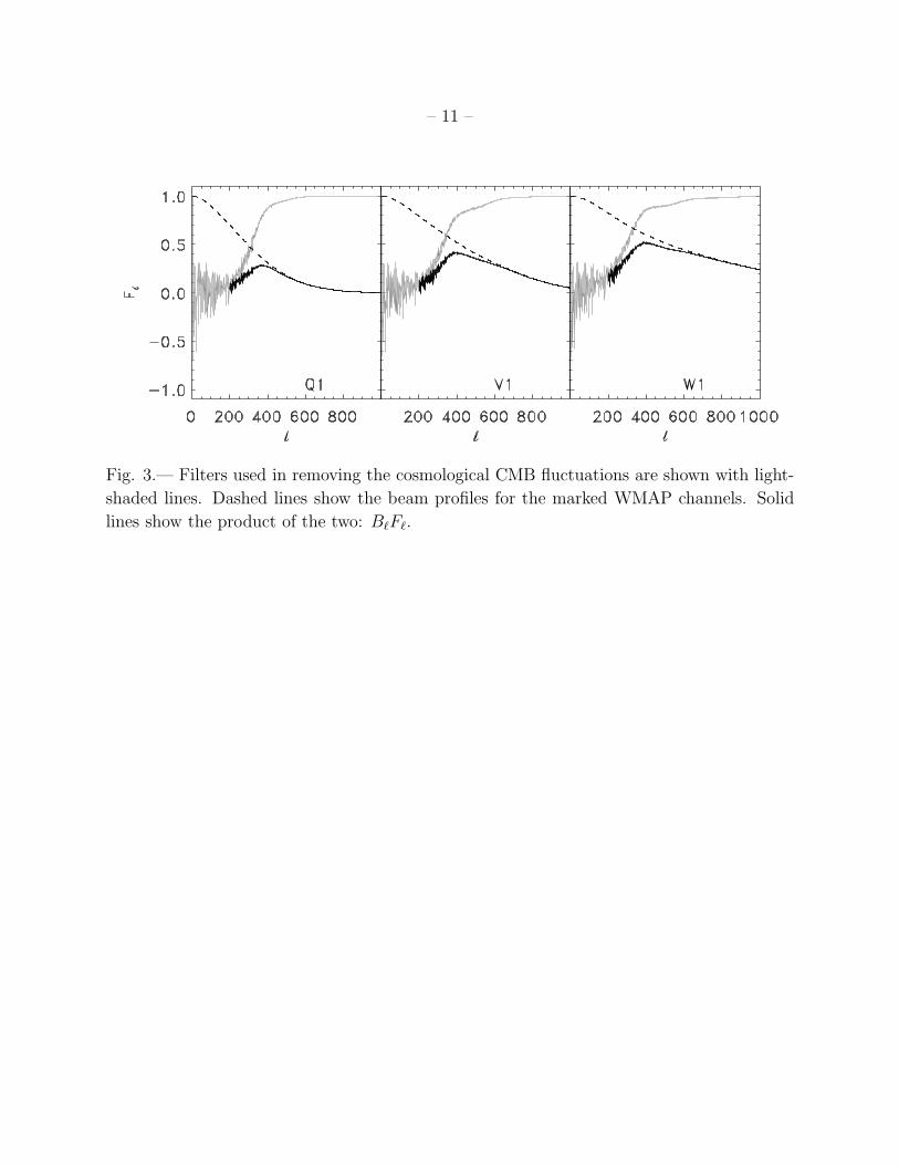
and the W channels the highest. The beam transfer functions for each channel, B, were

obtained from the same URL. The beam is also different in each channel with Q1 having the

poorest resolution and W4 the highest. Examples of the beam profile are shown in Fig. 3.

The maps were masked of foreground emitters using the KP2 and KP0 masks.

The resolution of the input maps is set by choosing Nside = 512 in HEALpix (Gorski et

al 2005). This corresponds to pixels of 4 × 10−6 sr (47.2 arcmin2) in area or θp 6.87′ on

the side. This resolution is much coarser than that of the X-ray maps used for constructing

our cluster catalog.

– 11 –

Fig. 3.— Filters used in removing the cosmological CMB fluctuations are shown with light-

shaded lines. Dashed lines show the beam profiles for the marked WMAP channels. Solid

lines show the product of the two: BF.

– 12 –

Because cosmological CMB fluctuations are correlated, they could leave a significant

variance in the noise component of our measurement (eq. 1) over the relatively few pixels

occupied by the clusters. Of course, this noise component will be the same, within its

standard deviation, for any other pixels in the maps, rather than being peculiar to the

cluster pixels. Because the power spectrum of this component, CΛCDM , is accurately known

from WMAP studies (Spergel et al 2007), it can be effectively filtered out of the CMB

maps, substantially reducing its contribution to the noise budget in eq. 1. This can be

achieved with the Wiener filter, which minimizes the mean square deviation from the noise

〈(δT − δnoise)2〉 (e.g. Press et al 1986). The Fourier transform of this filter is:

F =C(sky) − CΛCDM

B

C(sky)(2)

where C(sky) is the Fourier transform of the sky which contains both the ΛCDM component

and the instrument noise.

– 13 –

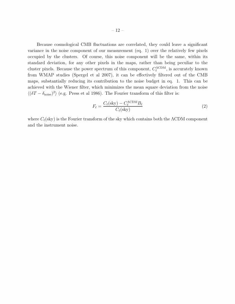
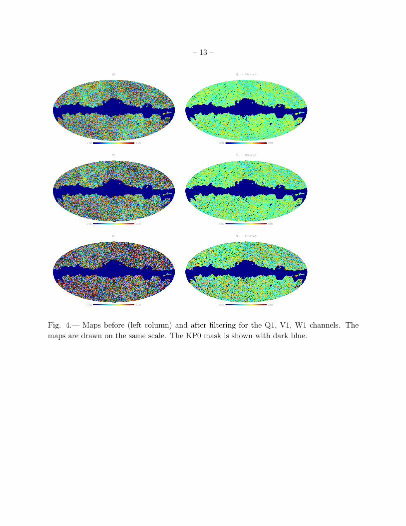
Fig. 4.— Maps before (left column) and after filtering for the Q1, V1, W1 channels. The

maps are drawn on the same scale. The KP0 mask is shown with dark blue.

– 14 –

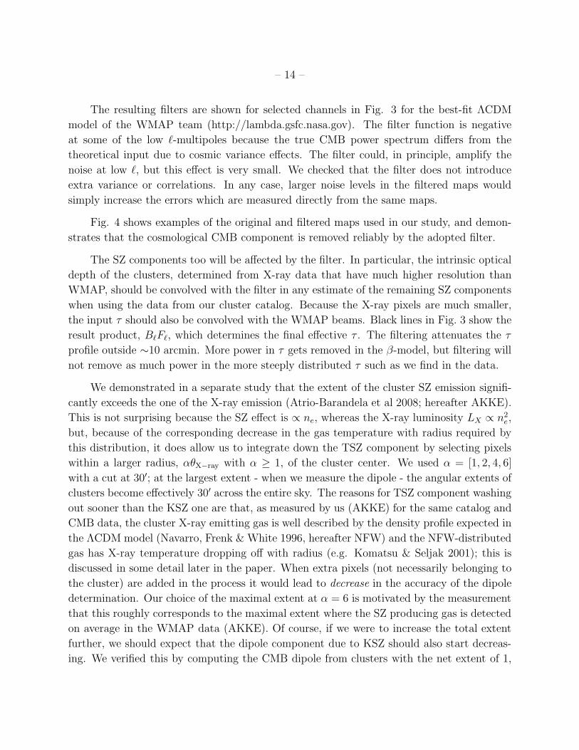
The resulting filters are shown for selected channels in Fig. 3 for the best-fit ΛCDM

model of the WMAP team (http://lambda.gsfc.nasa.gov). The filter function is negative

at some of the low -multipoles because the true CMB power spectrum differs from the

theoretical input due to cosmic variance effects. The filter could, in principle, amplify the

noise at low , but this effect is very small. We checked that the filter does not introduce

extra variance or correlations. In any case, larger noise levels in the filtered maps would

simply increase the errors which are measured directly from the same maps.

Fig. 4 shows examples of the original and filtered maps used in our study, and demon-

strates that the cosmological CMB component is removed reliably by the adopted filter.

The SZ components too will be affected by the filter. In particular, the intrinsic optical

depth of the clusters, determined from X-ray data that have much higher resolution than

WMAP, should be convolved with the filter in any estimate of the remaining SZ components

when using the data from our cluster catalog. Because the X-ray pixels are much smaller,

the input τ should also be convolved with the WMAP beams. Black lines in Fig. 3 show the

result product, BF, which determines the final effective τ . The filtering attenuates the τ

profile outside ∼10 arcmin. More power in τ gets removed in the β-model, but filtering will

not remove as much power in the more steeply distributed τ such as we find in the data.

We demonstrated in a separate study that the extent of the cluster SZ emission signifi-

cantly exceeds the one of the X-ray emission (Atrio-Barandela et al 2008; hereafter AKKE).

This is not surprising because the SZ effect is ∝ ne, whereas the X-ray luminosity LX ∝ n2e,

but, because of the corresponding decrease in the gas temperature with radius required by

this distribution, it does allow us to integrate down the TSZ component by selecting pixels

within a larger radius, αθX−ray with α ≥ 1, of the cluster center. We used α = [1, 2, 4, 6]

with a cut at 30′; at the largest extent - when we measure the dipole - the angular extents of

clusters become effectively 30′ across the entire sky. The reasons for TSZ component washing

out sooner than the KSZ one are that, as measured by us (AKKE) for the same catalog and

CMB data, the cluster X-ray emitting gas is well described by the density profile expected in

the ΛCDM model (Navarro, Frenk & White 1996, hereafter NFW) and the NFW-distributed

gas has X-ray temperature dropping off with radius (e.g. Komatsu & Seljak 2001); this is

discussed in some detail later in the paper. When extra pixels (not necessarily belonging to

the cluster) are added in the process it would lead to decrease in the accuracy of the dipole

determination. Our choice of the maximal extent at α = 6 is motivated by the measurement

that this roughly corresponds to the maximal extent where the SZ producing gas is detected

on average in the WMAP data (AKKE). Of course, if we were to increase the total extent

further, we should expect that the dipole component due to KSZ should also start decreas-

ing. We verified this by computing the CMB dipole from clusters with the net extent of 1,

– 15 –

2 and 3 degrees. (With this catalog, we cannot go further since the clusters’ overlap starts

getting in the way; e.g. at 3 the clusters already occupy ∼ 35% os the available sky). The

decrease in the dipole component is shown in Fig. 10 and discussed in detail in Sec. 6.

Wiener filtering reduces the TSZ temperature decrement and optical depth for each

cluster. When extending the analysis up to the largest extent (practically 30′ radius) we

find that the TSZ is diluted by noise and reduced to zero. Since clusters are not randomly

distributed on the sky the TSZ signal will give rise to a non-trivial dipole signature that,

in principle, may confuse the KSZ dipole. Nevertheless, the dipole generated by the cross

talk with the monopole cannot exceed the former, i.e. it must be aTSZ0 > aTSZ

1m , for all m; it

is shown below (Table 3) that this component is small. The following section describes the

results of the various simulations which support this statement.

5. Error estimation

Each of the eight CMB channel maps is processed separately. In the final maps, we set all

pixels to zero that fall outside of both the cluster areas and the mask and then compute the

dipole for each band using the remove dipole procedure in the standard HEALPix package.

Errors are computed from the pixels not associated with clusters as described below. The

results from each channel are added after weighting with their respective uncertainties.

We have estimated the errors with two different methods in order to account for both

the effects of the KP0 mask and the intrinsic distribution of the cluster samples in different

redshift bins: 1) At each z-bin we select new random pixels equal to the number of clusters

in each of the eight WMAP channel maps. These new pseudo-cluster centers are iteratively

selected to lie outside the KP0 mask and away from any of the true cluster pixels. They are

then assigned the cluster radii from the cluster catalog and the WMAP pixels are selected

within these new pseudo-clusters to compute the new dipole. We then ran 1,000 realizations

computing the errors to within a few percent accuracy. This method accounts for the effects

induced by the geometry of the KP0 mask. 2) In the second method, we keep the clusters

fixed at their celestial coordinates. The CMB maps for each of the eight channels are then

Fourier transformed and their power spectrum C computed and corrected for the fraction

of the sky occupied by the KP0 mask. We use this power spectrum to generate new random

phases in the corresponding am’s, which are then transformed back into the new CMB sky

maps, Tnew(θ, φ). In the new sky maps we select pixels occupied by the real clusters and

compute the resulting dipole. This method accounts for the effects induced by the possible

leakage from noise and residual CMB due to the intrinsic distribution of the cluster sample

in each z-bin.

– 16 –

The two methods give mean zero dipoles with errors that coincide to within a few

percent of each other, which is consistent with the cluster distribution not confusing the

final measurement.

– 17 –

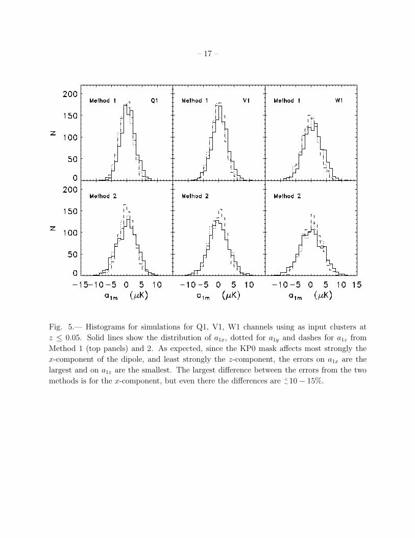
Fig. 5.— Histograms for simulations for Q1, V1, W1 channels using as input clusters at

z ≤ 0.05. Solid lines show the distribution of a1x, dotted for a1y and dashes for a1z from

Method 1 (top panels) and 2. As expected, since the KP0 mask affects most strongly the

x-component of the dipole, and least strongly the z-component, the errors on a1x are the

largest and on a1z are the smallest. The largest difference between the errors from the two

methods is for the x-component, but even there the differences are <∼10 − 15%.

– 18 –

Fig. 5 shows an example of the distribution of the dipole components from 1,000 sim-

ulations using random pixel locations in the maps. The figure shows that, as expected, the

distribution of a1m is Gaussian with zero mean, and that the cosmological CMB component

is removed efficiently. The effects of the CMB mask are such that the largest uncertainty is

for the a1x component of the dipole and the smallest is for a1z. From these simulations we

find that the noise terms for a1m integrate down approximately as ∝ N−1/2cl α−1, as expected

if the CMB component is indeed filtered out efficiently. Furthermore, we have established

that, compared to the first-year WMAP data, the uncertainties in a1m have decreased by

the expected factor of√

3. Since the noise terms are proportional to t−1/2, the final 8-year

WMAP data should further improve the measurement.

– 19 –

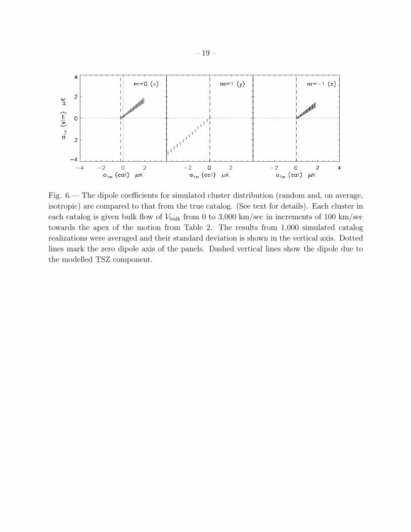
Fig. 6.— The dipole coefficients for simulated cluster distribution (random and, on average,

isotropic) are compared to that from the true catalog. (See text for details). Each cluster in

each catalog is given bulk flow of Vbulk from 0 to 3,000 km/sec in increments of 100 km/sec

towards the apex of the motion from Table 2. The results from 1,000 simulated catalog

realizations were averaged and their standard deviation is shown in the vertical axis. Dotted

lines mark the zero dipole axis of the panels. Dashed vertical lines show the dipole due to

the modelled TSZ component.

– 20 –

In order to assess that there is no cross-talk between the remaining monopole and dipole

which may confuse the measured KSZ dipole, we conducted the following experiment: 1)

The TSZ and KSZ components from the catalog clusters were modelled as described below

in Sec. 6. To exaggerate the effect of the cross-talk from the TSZ component, the latter

was normalized to the maximal measured monopole given in Table 3 for the bins where

a statistically significant dipole is detected (−1.3µK after filtering; for comparison Fig. 6

shows the results for the entire catalog, where the measured monopole is 0 ± 0.2µK). For

the KSZ component each cluster was given a bulk velocity, Vbulk, in the direction specified

in Table 2, whose amplitude varied from 0 to 3,000 km/sec in 31 increments of 100 km/sec.

The resultant CMB map was then filtered and the CMB dipole, a1m(cat), over the cluster

pixels computed for each value of Vbulk. 2) At the second stage we randomized cluster

positions with (l, b) uniformly distributed on celestial sphere over the full sky for a net of

1,000 realizations for each value of Vbulk (31,000 in total). This random catalog keeps the

same cluster parameters, but the cluster distribution now occupies the full sky (there is

now no mask) and on average does not have the same levels of anisotropy as the original

catalog. We then assigned each cluster the same bulk flow and computed the resultant CMB

dipole, a1m(sim), for each realization. The final a1m(sim) were averaged and their standard

deviation evaluated. Fig. 6 shows the comparison between the two dipoles for each value of

Vbulk. One can see that there is no significant offset in the CMB dipole produced by either

the mask or the cluster true sky distribution. The two sets of dipole coefficients are both

linearly proportional to Vbulk and to each other; in the absence of any bulk motion we recover

to a good accuracy the small value of the TSZ dipole. The most noticeable offset is for the

x-component of the dipole which is most affected by the mask, but even here the absolute

value of that offset is negligible. In principle, since the bulk flow motion is fixed in direction

and the cluster distribution is random, one expects the calibration factor defined below in

Sec. 8, C1,100 which translates the dipole in µK into velocity in km/sec, to be different from

one realization to the next, e.g. in some realizations certain clusters may be more heavily

concentrated in a plane perpendicular to the bulk flow motion and the measured C1,100 would

be smaller. In our case, the mean C1,100 differs by <∼10% suggesting that our catalog cluster

distribution is close to the mean cluster distribution in the simulations. This difference in

the overall normalization would only affect our translation of the dipole in µK into Vbulk in

km/sec.

Finally, we note that the errors computed this way are largely uncorrelated. For each

subsequent z-bin we add significantly more new cluster pixels, but the computed dipole,

of course, includes the clusters in the preceding bins. On the other hand, the errors are

computed from random positions on the maps and every realization contains, on average,

a completely new set of pixels. There may be some correlations between the various dipole

– 21 –

component errors produced by the mask, but as Figs. 5,6 show these correlated components

of the errors are small.

6. Results

6.1. Results by frequency band

Table 1 shows the measured dipole in the various redshift bins and shells for each of the

three frequency channels (Q, V, W), combining the numbers from each of the differential

assemblies (DA) with weights obtained from the simulations. One can see that the dipole

amplitude is such that the measurement becomes statistically significant for Ncl>∼300 for the

WMAP data noise levels. The dipole appears at the negligible monopole component when

computed from the clusters WMAP pixels. By itself this shows that it cannot originate from

the TSZ component. Nevertheless we also briefly discuss its spectral energy distribution in

as far as it relates to the KSZ origin of the measured dipole.

The KSZ and TSZ components have different frequency dependence potentially allowing

to distinguish the two origins of the measured dipole. When CMB photons are scattered

by the hot X-ray gas, the evolution of their occupation number, n, is described by the

Kompaneets equation: ∂n∂y

= 1x2

∂∂x

[x4(∂n∂x

+ n + n2)]. Here x ≡ hPν/kBTCMB and y is the

comptonization parameter. In the limit of y 1 and for the initially black-body radiation,

n = 1/[exp(x)−1], this equation specifies the change in the photon spectrum as (e.g. Stebbins

1997):

∆n yx exp(x)

[exp(x) − 1]2[xcoth

x

2− 4] (3)

As expected the distortion, ∆n, vanishes at high frequency limit (x → ∞). The WMAP

measurements are done in the Rayleigh-Jeans regime and the CMB temperature in K is

related to the measured flux, the spectral density Iν = 2hPν3

c2n in Jy/sr, via the antenna

temperature TCMB = c2

2kBν2 Iν ; the temperature distortion is ∆T = hPνkB

∆n. Combining this

with the above expression for ∆n, leads to the TSZ spectrum given by ∆TTSZ/TCMB = yG(x)

with:

G(x) =x2 exp(x)

[exp(x) − 1]2[xcoth

x

2− 4] (4)

The expression gives G(x) which is close to −2 for low frequencies, vanishes near 217 GHz,

goes positive at higher frequencies decreasing to zero again at the highest frequencies. For

the WMAP Q, V, W bands this expression gives: G(x) −1.84,−1.65,−1.25. Additionally,

there may be non-thermal components and relativistic corrections (Birkinshaw 1999).

– 22 –

Similarly, the KSZ spectrum can be shown to be given by ∆TKSZ/TCMB = τ vcH(x) with:

H(x) =x2 exp(x)

[exp(x) − 1]2(5)

The KSZ spectrum is much flatter over the WMAP frequencies with H(x) = 0.95, 0.9, 0.8

over the Q, V, W bands.

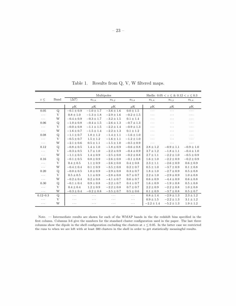
The dipole values in Table 1 are flat across the WMAP frequencies, from 40 to 94 GHz

and and are consistent with the spectrum expected from the KSZ component, although the

present data also give acceptable χ2 for the TSZ spectrum. Decreasing the noise by ∼ 2

expected from the future WMAP measurements may help distinguish the two components.

– 23 –

Table 1. Results from Q, V, W filtered maps.

Multipoles Shells: 0.05 < z ≤ & 0.12 < z ≤ 0.3

z ≤ Band 〈∆T 〉 a1,x a1,y a1,z a1,x a1,y a1,z

µK µK µK µK µK µK µK

0.05 Q −0.1 ± 0.9 −1.0 ± 1.7 −3.6 ± 1.6 0.0 ± 1.5 · · · · · · · · ·· · · V 0.8 ± 1.0 −1.3 ± 1.8 −2.9 ± 1.6 −0.2 ± 1.5 · · · · · · · · ·· · · W −0.4 ± 0.9 −0.3 ± 1.7 −3.2 ± 1.5 0.1 ± 1.4 · · · · · · · · ·0.06 Q −1.0 ± 0.8 −0.4 ± 1.5 −2.6 ± 1.3 −0.7 ± 1.3 · · · · · · · · ·· · · V −0.0 ± 0.8 −1.1 ± 1.5 −2.2 ± 1.4 −0.9 ± 1.3 · · · · · · · · ·· · · W −1.6 ± 0.7 −1.5 ± 1.4 −2.2 ± 1.3 0.1 ± 1.2 · · · · · · · · ·0.08 Q −1.1 ± 0.7 1.8 ± 1.2 −1.4 ± 1.1 −1.6 ± 1.0 · · · · · · · · ·· · · V −0.5 ± 0.7 1.5 ± 1.2 −1.6 ± 1.1 −1.2 ± 1.0 · · · · · · · · ·· · · W −2.1 ± 0.6 0.5 ± 1.1 −1.5 ± 1.0 −0.5 ± 0.9 · · · · · · · · ·0.12 Q −0.8 ± 0.5 1.4 ± 1.0 −1.8 ± 0.9 −0.6 ± 0.8 2.8 ± 1.2 −0.9 ± 1.1 −0.9 ± 1.0

· · · V −0.3 ± 0.5 1.7 ± 1.0 −2.2 ± 0.9 −0.4 ± 0.9 3.7 ± 1.2 −1.8 ± 1.1 −0.4 ± 1.0

· · · W −1.1 ± 0.5 1.4 ± 0.9 −2.5 ± 0.8 −0.2 ± 0.8 2.7 ± 1.1 −2.2 ± 1.0 −0.5 ± 0.9

0.16 Q −0.1 ± 0.5 0.8 ± 0.9 −2.6 ± 0.8 −0.1 ± 0.8 1.6 ± 1.0 −2.2 ± 0.9 −0.2 ± 0.9

· · · V 0.4 ± 0.5 1.1 ± 0.9 −2.6 ± 0.8 0.4 ± 0.8 2.3 ± 1.1 −2.6 ± 0.9 0.6 ± 0.9

· · · W −0.4 ± 0.4 0.1 ± 0.9 −3.5 ± 0.8 0.2 ± 0.7 0.5 ± 1.0 −3.7 ± 0.9 0.1 ± 0.8

0.20 Q −0.0 ± 0.5 1.0 ± 0.9 −2.9 ± 0.8 0.3 ± 0.7 1.8 ± 1.0 −2.7 ± 0.9 0.5 ± 0.8

· · · V 0.5 ± 0.5 1.1 ± 0.9 −2.8 ± 0.8 0.7 ± 0.7 2.2 ± 1.0 −2.9 ± 0.9 1.0 ± 0.8

· · · W −0.2 ± 0.4 0.2 ± 0.8 −4.1 ± 0.7 0.6 ± 0.7 0.6 ± 0.9 −4.4 ± 0.9 0.6 ± 0.8

0.30 Q −0.1 ± 0.4 0.9 ± 0.8 −2.2 ± 0.7 0.4 ± 0.7 1.6 ± 0.9 −1.9 ± 0.8 0.5 ± 0.8

· · · V 0.4 ± 0.4 1.2 ± 0.9 −2.2 ± 0.8 0.7 ± 0.7 2.2 ± 0.9 −2.2 ± 0.8 1.0 ± 0.8

· · · W −0.3 ± 0.4 −0.2 ± 0.8 −3.5 ± 0.7 0.5 ± 0.6 0.1 ± 0.9 −3.7 ± 0.8 0.5 ± 0.7

0.12–0.3 Q · · · · · · · · · · · · 0.8 ± 1.4 −2.9 ± 1.3 2.3 ± 1.2

· · · V · · · · · · · · · · · · 0.9 ± 1.5 −2.2 ± 1.3 3.1 ± 1.2

· · · W · · · · · · · · · · · · −2.2 ± 1.4 −5.2 ± 1.3 1.9 ± 1.2

Note. — Intermediate results are shown for each of the WMAP bands in the the redshift bins specified in the

first column. Columns 3-6 give the numbers for the standard cluster configuration used in the paper. The last three

columns show the dipole in the shell configuration excluding the clusters at z ≤ 0.05. In the latter case we restricted

the runs to when we are left with at least 300 clusters in the shell in order to get statistically meaningful results.

– 24 –

As a further consistency check and to estimate how much of the signal is contributed by

the farthest clusters, we have also computed the numbers in a shell configuration excluding

clusters with z ≤ 0.05 and for the 274 clusters with 0.12 ≤ z ≤ 0.3. Interpretation of such

numbers can be cumbersome because of the complicated window involved, but nevertheless

they can provide a useful diagnostic of the consistency of the results and the contribution

to the dipole by the farthest clusters. Our results show that we start getting statistically

meaningful results with at least ∼ 300 clusters, so the runs were done for the bins where

the outer z exceeded 0.012. The dipole coefficients for each band are shown in the last three

columns of Table 1. They are overall consistent with the main results and provide further

support that the dipole is generated by cluster motions on the largest scales.

– 25 –

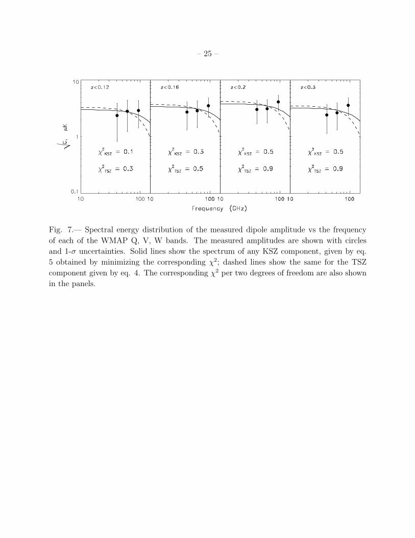
Fig. 7.— Spectral energy distribution of the measured dipole amplitude vs the frequency

of each of the WMAP Q, V, W bands. The measured amplitudes are shown with circles

and 1-σ uncertainties. Solid lines show the spectrum of any KSZ component, given by eq.

5 obtained by minimizing the corresponding χ2; dashed lines show the same for the TSZ

component given by eq. 4. The corresponding χ2 per two degrees of freedom are also shown

in the panels.

– 26 –

Fig. 7 plots the dipole amplitude for four farthest redshift bins vs the frequency of each

channel juxtaposed against the TSZ energy spectrum normalized to the measured dipole

at 40 GHz. The TSZ spectrum (eq. 4 below) would predict a smaller dipole value in the

W band. On the other hand, the spectrum of the dipole arising from the KSZ should be

approximately flat across the frequencies consistent with the plotted numbers (as mentioned

above and shown in the figure the TSZ spectrum also gives acceptable χ2 given the noise in

the present WMAP data).

6.2. Results averaged over all frequency channels.

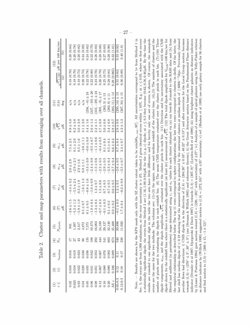
Table 2 shows the results after weight-averaging over all of the eight DA’s. The table

also gives additional information on the cluster samples used in each measurement. In or-

der to assess the potential impact of cooling flows on the results, we have also made the

computations omitting cluster central pixels in WMAP data. The results were essentially

unchanged compared to those presented in the table. There is a clear statistically-significant

dipole at the level of ∼ 2 − 3µK once we reach ∼ 300 clusters and the aperture ( 30′) en-

compassing most of the hot gas producing the SZ effect. The dipole remains as the monopole

representing the mean TSZ component from hot gas within the selected aperture vanishes.

– 27 –

Tab

le2.

Clu

ster

and

map

par

amet

ers

wit

hre

sult

sfr

omav

erag

ing

over

allch

annel

s.

(1)

(2)

(3)

(4)

(5)

(6)

(7)

(8)

(9)

(10)

(11)

(12)

z≤

〈z〉

z media

nN

cl

Npix

els

〈T〉

a1,x

a1,y

a1,z

√C

1(l

,b)

√C

1,1

00:

µK

per

100

km

/se

c

µK

µK

µK

µK

µK

deg

(a)

(b)

0.0

20.0

16

0.0

16

17

941

−2.6

±1.5

−4.4

±3.2

2.0

±2.9

7.5

±2.5

8.9

±5.0

n/a

0.1

8(0

.70)

0.2

0(0

.84)

0.0

25

0.0

18

0.0

19

27

1,4

97

−5.2

±1.2

−5.5

±2.4

−2.9

±2.1

0.1

±2.0

6.2

±3.8

n/a

0.1

8(0

.70)

0.2

0(0

.78)

0.0

30.0

22

0.0

23

43

2,4

17

−5.9

±1.0

0.3

±1.9

2.9

±1.6

0.5

±1.6

3.0

±2.9

n/a

0.1

8(0

.73)

0.2

0(0

.82)

0.0

40.0

29

0.0

30

86

4,8

72

0.5

±0.7

−1.6

±1.3

0.8

±1.1

−2.6

±1.1

3.1

±2.0

n/a

0.2

0(0

.73)

0.2

4(0

.89)

0.0

50.0

35

0.0

36

135

7,5

75

0.1

±0.5

−0.8

±1.0

−3.3

±0.9

−0.0

±0.9

3.4

±1.6

(256,−

0)±

24

0.2

2(0

.76)

0.2

4(0

.82)

0.0

60.0

41

0.0

42

188

10,4

74

−1.0

±0.4

−1.0

±0.9

−2.4

±0.8

−0.5

±0.7

2.6

±1.4

(247,−

10)±

26

0.2

2(0

.80)

0.2

2(0

.79)

0.0

80.0

51

0.0

53

292

16,0

64

−1.3

±0.4

1.3

±0.7

−1.5

±0.6

−1.1

±0.6

2.2

±1.1

(310,−

29)±

24

0.2

4(0

.76)

0.2

6(0

.83)

0.1

20.0

67

0.0

67

444

24,1

89

−0.7

±0.3

1.5

±0.6

−2.2

±0.5

−0.4

±0.5

2.7

±0.9

(305,−

9)±

17

0.2

6(0

.79)

0.2

8(0

.88)

0.1

60.0

80

0.0

76

541

29,1

27

−0.1

±0.3

0.7

±0.5

−2.9

±0.5

0.1

±0.4

3.0

±0.8

(283,3

)±

13

0.2

5(0

.75)

0.2

7(0

.83)

0.2

00.0

90

0.0

82

603

32,1

46

0.1

±0.3

0.7

±0.5

−3.3

±0.4

0.5

±0.4

3.4

±0.8

(282,9

)±

11

0.2

8(0

.84)

0.2

9(0

.90)

All

z0.1

06

0.0

89

674

35,4

09

0.0

±0.2

0.6

±0.5

−2. 7

±0.4

0.6

±0.4

2.8

±0.7

(283,1

1)±

14

0.2

9(0

.965)

0.3

2(1

.01)

0.0

5-0

.30.1

20.1

1540

29,8

96

−0.1

±0.3

1.2

±0.5

−2.6

±0.5

0.7

±0.4

2.9

±0.8

(295,1

4)±

13

0.3

1(0

.84)

0.3

3(0

.92)

0.1

2-0

.30.1

80.1

7230

11,9

20

1.7

±0.4

−0.2

±0.8

−3.5

±0.7

2.4

±0.7

4.2

±1.3

(267,3

4)±

15

0.3

6(0

.89)

0.4

0(1

.0)

Note

.—

Res

ult

sare

show

nfo

rth

eK

P0

mask

only

wit

hth

eSZ

clust

erex

tent

taken

tobe

min

[6θ X

−ra

y,3

0′ ].

All

unce

rtain

ties

corr

espond

to1σ

from

Met

hod

1in

Sec

.5;th

eer

rors

are

from

1,0

00

realiza

tions,

soth

eer

ror

unce

rtain

tyis

4%

.M

ethod

2giv

esid

enti

caler

rors

wit

hin

< ∼10%

.E

.g.:

at

z≤

0.0

5,w

her

ew

efirs

tre

cover

ast

ati

stic

ally

signifi

cant

dip

ole

,th

eer

rors

from

Met

hod

2are

(1.1

6,1

.09,0

.94)µ

Kfo

rth

e(x

,y,z

)dip

ole

;at

z≤

0.3

they

bec

om

e(0

.62,0

.56,0

.46)µ

K.B

yth

etim

eth

e

resu

lts

are

rounded

toone

signifi

cant

dig

itin

the

table

the

two

sets

hav

elitt

lediff

eren

ceand

for

bre

vity

only

one

set

of

erro

rsis

show

n.

Of

cours

e,th

em

onopole

erro

rsare

the

sam

efo

rth

etw

om

ethods.

The

colu

mns

are

:(1

)-(3

)th

eupper

,m

ean

and

med

ian

redsh

ift

of

the

clust

erbin

s.(4

),(5

)T

he

num

ber

of

clust

ers

and

the

num

ber

of

pix

els

use

din

evalu

ati

ng

the

dip

ole

inea

chre

dsh

ift

bin

.(6

)T

he

mea

nC

MB

tem

per

atu

reev

alu

ate

dov

erth

ecl

ust

erpix

els

inea

chbin

.(7

)-(1

0)

Thre

e

dip

ole

com

ponen

ts,

a1m

,and

the

dip

ole

am

plitu

de,

√C

1,

evalu

ate

dov

erth

ecl

ust

erpix

els

inea

chbin

.(1

1)

Dir

ecti

on

and

its

unce

rtain

tyass

oci

ate

dw

ith

the

CM

B

dip

ole

show

nfo

rth

ere

dsh

ift

bin

sw

her

eth

ere

isa

statist

ically

signifi

cant

(at

least

2σ)

mea

sure

men

tof√

C1.

(12)

The

tota

ldip

ole

am

plitu

de

for

Vbulk

=100

km

/se

cfo

r

filt

ered

and

unfilt

ered

(in

pare

nth

eses

)m

aps

det

erm

ined

usi

ng

r cand

ne

valu

esfo

rea

chcl

ust

erobta

ined

via

(a)

our

bes

t-fit

β-m

odel

toth

eR

ASS

data

and

(b)

from

the

empir

icalre

lati

onsh

ipas

des

crib

edbel

owT

he

top

11

row

sco

rres

pond

tosp

her

eco

nfigura

tions;

the

last

two

row

sco

rres

pond

tocl

ust

ers

insh

ells

.O

fth

ela

tter

,th

e

last

shel

lhas

med

ian

dip

ole

of

0.1

8sh

owin

gth

at

the

mea

sure

ddip

ole

ispro

duce

dby

the

oute

rmost

clust

ers

at

med

ian

dep

thof

> ∼600h−

1M

pc.

Pre

vio

usl

ycl

aim

ed

pec

uliar

flow

shad

dir

ecti

ons:

i)C

MB

dip

ole

isin

the

dir

ecti

on

of

(l,b

)=

(264.2

6±

0.3

3,4

8.2

2±

0.1

3)

and

aft

erco

rrec

tion

for

the

Loca

lG

roup

moti

on

bec

om

es

tow

ard

s(l

,b)

=(2

76±

3,3

0±

3)

(see

(Str

auss

&W

illick

1995)

and

refe

rence

sth

erei

n);

ii)

the

Gre

at

Att

ract

or

motion

base

don

the

Fundam

enta

lP

lane

dis

tance

indic

ato

r(D

ress

ler

etal1987;D

jorg

ovsk

i&

Dav

is1987)

isto

ward

s(l

,b)

=(3

07,9

)(L

ynden

-Bel

let

al1988);

iii)

usi

ng

bri

ghte

stcl

ust

ergala

xie

sas

dis

tance

indic

ato

rs

by

(Lauer

&Post

man

1994)

gav

em

oti

on

tow

ard

(l,b

)=

(220,−

28)

wit

hunce

rtain

tyof±

27;iv

)A

naly

sis

ofa

sam

ple

ofsp

iralgala

xie

susi

ng

the

Tully-F

isher

rela

tion

as

dis

tance

indic

ato

rby

(Willick

1999)

sugges

ted

moti

on

to(l

,b)

=(2

72,1

0)

wit

h±

35

unce

rtain

ty;v)

ref.

(Hudso

net

al1999)

use

earl

ygala

xy

sam

ple

for

56

clust

ers

and

find

moti

on

to(l

,b)

=(2

60±

15,−

1±

12)

.

– 28 –

The direction of the dipole and its uncertainty in Table 2 were computed as follows:

each dipole component is assumed Gaussian-distributed, with the given mean and errors.

At each z we generate 104 dipoles from a normal distribution with the standard deviation

equal to each component error bar and compute the angle of these dipoles with respect to

the direction of the mean dipole. For small angles, this angle follows a χ2 distribution with 3

degrees of freedom; the uncertainty in the table corresponds to the 68 % confidence contour

of this distribution. The directions from previous measurements of peculiar flows based on

galaxy distance indicators and those of the acceleration dipoles of the various cluster studies

are summarized in the note to Table 2. The direction of the bulk flow deduced here is ∼ 20

from the “global CMB dipole” direction, with a 1-σ error of ∼ 10-25 over the range of z

probed in this study, and does not vary significantly within the range covered by our data.

– 29 –

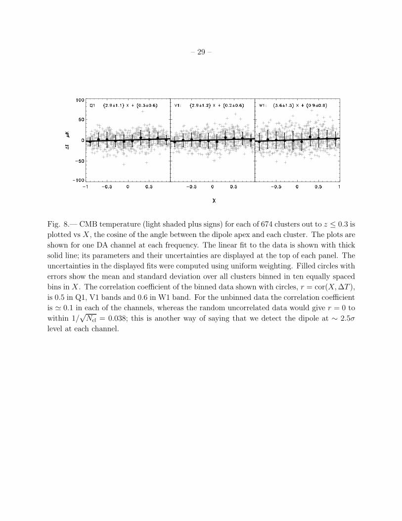
Fig. 8.— CMB temperature (light shaded plus signs) for each of 674 clusters out to z ≤ 0.3 is

plotted vs X, the cosine of the angle between the dipole apex and each cluster. The plots are

shown for one DA channel at each frequency. The linear fit to the data is shown with thick

solid line; its parameters and their uncertainties are displayed at the top of each panel. The

uncertainties in the displayed fits were computed using uniform weighting. Filled circles with

errors show the mean and standard deviation over all clusters binned in ten equally spaced

bins in X. The correlation coefficient of the binned data shown with circles, r = cor(X, ∆T ),

is 0.5 in Q1, V1 bands and 0.6 in W1 band. For the unbinned data the correlation coefficient

is 0.1 in each of the channels, whereas the random uncorrelated data would give r = 0 to

within 1/√

Ncl = 0.038; this is another way of saying that we detect the dipole at ∼ 2.5σ

level at each channel.

– 30 –

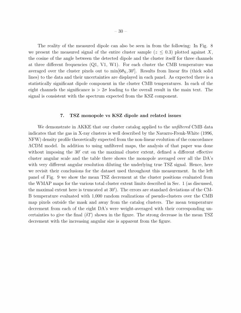
The reality of the measured dipole can also be seen in from the following: In Fig. 8

we present the measured signal of the entire cluster sample (z ≤ 0.3) plotted against X,

the cosine of the angle between the detected dipole and the cluster itself for three channels

at three different frequencies (Q1, V1, W1). For each cluster the CMB temperature was

averaged over the cluster pixels out to min[6θX, 30′]. Results from linear fits (thick solid

lines) to the data and their uncertainties are displayed in each panel. As expected there is a

statistically significant dipole component in the cluster CMB temperatures. In each of the

eight channels the significance is > 2σ leading to the overall result in the main text. The

signal is consistent with the spectrum expected from the KSZ component.

7. TSZ monopole vs KSZ dipole and related issues

We demonstrate in AKKE that our cluster catalog applied to the unfiltered CMB data

indicates that the gas in X-ray clusters is well described by the Navarro-Frenk-White (1996,

NFW) density profile theoretically expected from the non-linear evolution of the concordance

ΛCDM model. In addition to using unfiltered maps, the analysis of that paper was done

without imposing the 30′ cut on the maximal cluster extent, defined a different effective

cluster angular scale and the table there shows the monopole averaged over all the DA’s

with very different angular resolution diluting the underlying true TSZ signal. Hence, here

we revisit their conclusions for the dataset used throughout this measurement. In the left

panel of Fig. 9 we show the mean TSZ decrement at the cluster positions evaluated from

the WMAP maps for the various total cluster extent limits described in Sec. 1 (as discussed,

the maximal extent here is truncated at 30′). The errors are standard deviations of the CM-

B temperature evaluated with 1,000 random realizations of pseudo-clusters over the CMB

map pixels outside the mask and away from the catalog clusters. The mean temperature

decrement from each of the eight DA’s were weight-averaged with their corresponding un-

certainties to give the final 〈δT 〉 shown in the figure. The strong decrease in the mean TSZ

decrement with the increasing angular size is apparent from the figure.

– 31 –

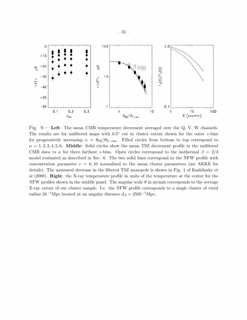
Fig. 9.— Left: The mean CMB temperature decrement averaged over the Q, V, W channels.The results are for unfiltered maps with 0.5 cut in cluster extent shown for the outer z-binsfor progressively increasing α = θSZ/θX−ray. Filled circles from bottom to top correspond toα = 1, 2, 3, 4, 5, 6. Middle: Solid circles show the mean TSZ decrement profile in the unfilteredCMB data vs α for three farthest z-bins. Open circles correspond to the isothermal β = 2/3model evaluated as described in Sec. 6. The two solid lines correspond to the NFW profile withconcentration parameter c = 6, 10 normalized to the mean cluster parameters (see AKKE fordetails). The measured decrease in the filtered TSZ monopole is shown in Fig. 1 of Kashlinsky etal (2008). Right: the X-ray temperature profile in units of the temperature at the center for theNFW profiles shown in the middle panel. The angular scale θ in arcmin corresponds to the averageX-ray extent of our cluster sample. I.e. the NFW profile corresponds to a single cluster of virialradius 2h−1Mpc located at an angular distance dA = 250h−1Mpc.

– 32 –

The middle panel of the figure shows the mean CMB temperature profile of the TSZ

decrement in the unfiltered maps for three outer redshift bins. (The decrease of the filtered

TSZ decrement profile is shown in Fig. 1 of Kashlinsky et al, 2008). The expectation from

the isothermal β-model for these bins was evaluated as described in Sec. 6 and is shown with

the open circles. It fits well the data at the cluster inner parts, but deviates strongly from

the measurements at larger radii. The fits from the NFW profiles using a method similar to

Komatsu & Seljak (2001) are shown with solid lines for two concentration parameters (see

AKKE for details). These profiles provide a good fit to the data.

It is important to emphasize in this context that the gas with the NFW profile which is in

hydrostatic equilibrium with the cluster gravitational field must have the X-ray temperature

decreasing with radius (Komatsu & Seljak 2001). This is confirmed by numerical simulations

of the cluster formation within the ΛCDM model (Borgani et al 2004) as well as by the

available observations of a few nearby clusters (Pratt et al 2007). The latter cannot yet

probe the TX profile all the way to the virial radius, but do show a decrease by a factor of

∼ 2 out to about half of it (see e.g. Fig. 5 of Pratt et al 2007). In the NFW profile the

gas density profile in the outer parts goes as ne ∝ r−3 with the polytropic index which is

approximately constant for all clusters at γ 1.2 (Komatsu & Seljak 2001). Thus the X-ray

temperature must drop at least as TX ∝ r−0.6 at the outer parts and for larger values of γ

the drop will be correspondingly more rapid. The temperature profile implied by the NFW

density profile normalized to the data in the middle panel is shown in the right panel of Fig.

9.

– 33 –

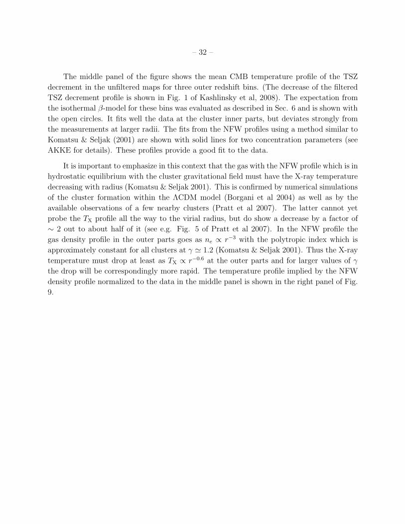
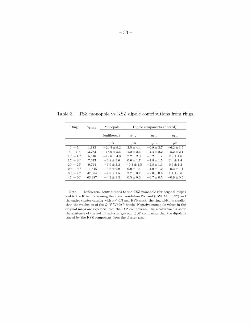
Table 3. TSZ monopole vs KSZ dipole contributions from rings.

Ring Npixels Monopole Dipole components (filtered)

(unfiltered) a1,x a1,y a1,z

µK µK µK µK

0′ − 5′ 1,183 −24.5 ± 9.2 3.5 ± 4.4 −0.9 ± 3.7 −6.2 ± 3.5

5′ − 10′ 3,283 −18.0 ± 5.5 1.2 ± 2.6 −4.4 ± 2.2 −5.2 ± 2.1

10′ − 15′ 5,546 −12.6 ± 4.3 2.2 ± 2.0 −5.2 ± 1.7 2.9 ± 1.6

15′ − 20′ 7,673 −6.8 ± 3.6 0.6 ± 1.7 −4.8 ± 1.5 2.0 ± 1.4

20′ − 25′ 9,744 −6.0 ± 3.2 −0.3 ± 1.5 −2.8 ± 1.3 0.5 ± 1.2

25′ − 30′ 11,845 −5.8 ± 2.9 0.9 ± 1.4 −1.0 ± 1.2 −0.3 ± 1.1

30′ − 45′ 47,064 −4.6 ± 1.5 2.7 ± 0.7 −2.0 ± 0.6 1.4 ± 0.6

45′ − 60′ 63,987 −4.3 ± 1.3 0.5 ± 0.6 −0.7 ± 0.5 −0.9 ± 0.5

Note. — Differential contributions to the TSZ monopole (for original maps)

and to the KSZ dipole using the lowest resolution W-band (FWHM 0.2) and

the entire cluster catalog with z ≤ 0.3 and KP0 mask; the ring width is smaller

than the resolution of the Q, V WMAP bands. Negative monopole values in the

original maps are expected from the TSZ component. The measurements show

the existence of the hot intracluster gas out >∼ 30′ confirming that the dipole is

traced by the KSZ component from the cluster gas.

– 34 –

The implications of the above are that in the outer parts of clusters the TSZ monopole

component must decrease faster than the KSZ dipole as we increase the aperture to probe

the cluster outer regions. This is what we observe in the data and allowed us to isolate the

KSZ dipole component as the TSZ monopole vanishes. The reason we present the results

out to min[6θX−ray, 30′] is that this is roughly the scale where we still detect statistically

significant TSZ signal in the unfiltered data (AKKE and Table 3 below).

Table 3 shows the differential distribution of the TSZ and dipole components in rings of

the specified radius and width around the clusters in our catalog. The data from the W-band

were selected for the table because this channel has the finest angular resolution making it

the most adequate to probe the differential contribution to the final signal. The table clearly

shows that in the unfiltered data the X-ray emitting gas producing the TSZ signal exists out

to at least 25′ − 30′, the effective final radius of our cluster catalog. The measurements in

the table confirm explicitly that, due to the X-ray temperature decrease, in the filtered maps

the dipole KSZ component can be isolated as the TSZ monopole vanishes. Mathematically,

discounting the additional TX factor with γ 1.2 − 1.3 in the TSZ terms makes the KSZ

term for the NFW-like clusters lie close to the TSZ profile of the isothermal β ∼ 2/3 model

and, hence, its KSZ decrease with increasing aperture radius should roughly mimic the open

circles in the middle panel of Fig. 9. Of course, the true cluster properties, such as the

electron density and X-ray temperature profiles, can be mathematically constrained (and

perhaps even recovered) from the measurements of both the KSZ dipole and TSZ monopole

profiles; this, however, lies outside the scope of this investigation.

– 35 –

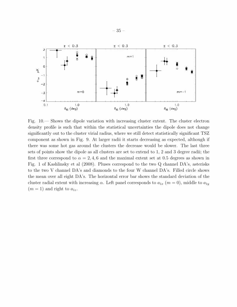
Fig. 10.— Shows the dipole variation with increasing cluster extent. The cluster electron

density profile is such that within the statistical uncertainties the dipole does not change

significantly out to the cluster virial radius, where we still detect statistically significant TSZ

component as shown in Fig. 9. At larger radii it starts decreasing as expected, although if

there was some hot gas around the clusters the decrease would be slower. The last three

sets of points show the dipole as all clusters are set to extend to 1, 2 and 3 degree radii; the

first three correspond to α = 2, 4, 6 and the maximal extent set at 0.5 degrees as shown in

Fig. 1 of Kashlinsky et al (2008). Pluses correspond to the two Q channel DA’s, asterisks

to the two V channel DA’s and diamonds to the four W channel DA’s. Filled circle shows

the mean over all eight DA’s. The horizontal error bar shows the standard deviation of the

cluster radial extent with increasing α. Left panel corresponds to a1x (m = 0), middle to a1y

(m = 1) and right to a1z .

– 36 –

Of course, as the the mean cluster extent gets increased further and we reach passed the

cluster gas extent radii we should also observe a decrease in the measured dipole. To check

this we have run our pipeline with the net cluster angular extent increased to 1, 2 and 3

degree radii. At the 3 radii the cluster catalog occupies a significant fraction of the available

sky, 35%, so at larger radii the clusters overlapping would become significant. We observe

that the dipole, in all z-bins where we have a statistically significant measurement, indeed

decreases with the increasing mean extent for the apertures with α>∼6. This is shown in Fig.

10. It is interesting to note that as we increase the extent further we may be detecting signs

of the two other components of the dipole (x, z), as testified by the small scatter among the

mean dipole from all the eight DA’s. This is because the noise, reflected in the scatter among

the eight DA’s, decreases faster than the dilution factor in the measured dipole. However,

it would be difficult to interpret these results with the current version of our X-ray catalog.

8. Calibration: translating µK into km/sec

In order to translate the CMB dipole in µK into the amplitude of Vbulk in km/sec, we

proceed as follows. First, we verified that our catalog reproduces accurately the measured

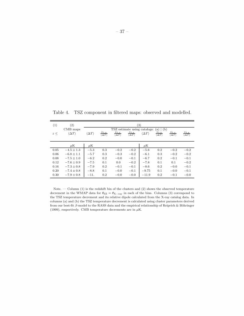
TSZ properties of the measured CMB parameters (see also Sec. 7). Table 4 compares the

directly determined TSZ contributions in the redshift bins where we have a statistically

significant detection of the dipole with those determined from the parameters in the catalog.

The latter is determined as follows: for each cluster we construct a TSZ map in each WMAP

channel using the catalog values for the electron density, core radius, X-ray temperature and

total extent, and assuming β = 2/3. These maps are then filtered using the filters shown in

Fig. 3 and coadded using the weights used in the main pipeline. As a consistency check we

determine the gas profile using two independent methods: (a) fitting a β-profile directly to

the RASS X-ray data, and (b) using an empirical relationship between the core radius and

X-ray luminosity. The quantities derived from the catalog should have the same uncertainties

(generated by the CMB maps noise etc) as those measured directly and for brevity are not

shown. The table shows that there is good agreement between the directly measured TSZ

component and that derived using the X-ray cluster catalog for θSZ = θX−ray. The two sets

of numbers mostly overlap at 1-σ level and always overlap at 2-σ. To further check that

the agreement is not accidental, we have generated a test catalog randomly assigning the

various cluster parameters from different clusters. The agreement completely disappears and

the two sets of numbers become different by factors of ∼ 2 − 3.

– 37 –

Table 4. TSZ component in filtered maps: observed and modelled.

(1) (2) (3)

CMB maps TSZ estimate using catalogs: (a) | (b)

z ≤ 〈∆T 〉 〈∆T 〉 a1,x〈∆T〉

a1,y〈∆T〉

a1,z〈∆T〉 〈∆T 〉 a1,x

〈∆T〉a1,y〈∆T〉

a1,z〈∆T〉

µK µK µK

0.05 −4.5 ± 1.3 −5.3 0.3 −0.2 −0.2 −5.6 0.2 −0.2 −0.2

0.06 −6.8 ± 1.1 −5.7 0.3 −0.3 −0.2 −6.1 0.3 −0.2 −0.2

0.08 −7.5 ± 1.0 −6.2 0.2 −0.0 −0.1 −6.7 0.2 −0.1 −0.1

0.12 −7.6 ± 0.9 −7.5 0.1 0.0 −0.2 −7.8 0.1 0.1 −0.2

0.16 −7.3 ± 0.8 −7.9 0.2 −0.1 −0.1 −8.6 0.2 −0.0 −0.1

0.20 −7.4 ± 0.8 −8.8 0.1 −0.0 −0.1 −9.75 0.1 −0.0 −0.1

0.30 −7.9 ± 0.8 −11. 0.2 −0.0 −0.0 −11.9 0.2 −0.1 −0.0

Note. — Column (1) is the redshift bin of the clusters and (2) shows the observed temperature

decrement in the WMAP data for θSZ = θX−ray in each of the bins. Columns (3) correspond to

the TSZ temperature decrement and its relative dipole calculated from the X-ray catalog data. In

columns (a) and (b) the TSZ temperature decrement is calculated using cluster parameters derived

from our best-fit β-model to the RASS data and the empirical relationship of Reiprich & Bohringer

(1999), respectively. CMB temperature decrements are in µK.

– 38 –

Thus the cluster properties in the catalog are determined reasonably well to estimate the

translation factor between the CMB dipole amplitude and the bulk flow velocity. To account

for the attenuation of the clusters’ τ values by both the beam and the filter, we convolve

the gas profile of each cluster with the beam and the filter shown in Fig. 3 over the WMAP

pixels associated with it. Each cluster is given a bulk flow motion of 100 km/sec in the

direction listed in Table 2, so that each pixel of the i-th cluster has δT = TCMBτi(θ)Vbulk/c,

with θ being the angular distance to the cluster center. We then compute the CMB dipole

of the resulting cluster map and average the results for each channel map with the same

weights as used in the dipole computation. This allows us to estimate the dipole amplitude,

C1,100, contributed by each 100 km/sec of bulk-flow. We restrict our calculation to the central

1θX−ray where the β-model and NFW profiles differ by 10-30% and where the central values of

the measured dipole are similar to the values measured at the final aperture extent. In other

words, we assume that for each cluster all pixels measure the same velocity (in modulus)

across the sky, so the calibration constant, measured from any subset of pixels is the same,

irrespective of the signal (in µK) measured at their location.

The results are shown in the last column of Table 2 for the central values of the direc-

tion of the measured flow; varying the direction within the uncertainties of (l, b) shown in

Table 2 changes the numbers by at most a few percent. A bulk flow of 100 km/sec thus

leads to√

C1 0.8µK for unfiltered clusters; this corresponds to an average optical depth

of our cluster sample of 〈τ〉 10−3 consistent with what is expected for a typical galaxy

cluster. Filtering reduces the effective τ by a factor of 3. As mentioned above, since a

β-model provides a poor fit to the measured TSZ component outside the estimated values

of θX−ray (Atrio-Barandela et al 2008), we compute C1,100 with the total extent assumed to

be θX−ray where the central value of the bulk-flow dipole has approximately the same value

as at the final aperture of min[6θX−ray, 30′]. Owing to the large size of our cluster sample

(Ncl ∼130-675), the random uncertainties in the estimated values of C1,100 should be small,

but we cannot exclude a systematic offset related to selection biases affecting our cluster

catalog at high redshift. Any such offset, if present, will become quantifiable with the next

version of our X-ray cluster catalog (in preparation) which will use the empirically estab-

lished SZ profile (Atrio-Barandela et al 2008) rather than the currently used β-model to

parameterize the cluster gas profile. The good agreement between the various TSZ-related

quantities shown in Table 4 for θSZ = θX−ray and the observed values for both unfiltered

(Atrio-Barandela et al 2008) and filtered maps suggests, however, that these systematic un-

certainties are not likely to be high. We also note that they only affect the accuracy of the

determination of the amplitude of the bulk flow, but cannot put its existence into doubt which

is established from the CMB dipole detected at the cluster locations. Since the filtering effec-

tively removes the profile outside, approximately, a few arcmin (see Fig. 3), it removes a more

– 39 –

substantial amount of power in the β-model when the cluster SZ extent is increased beyond

θX−ray, than in the steeper profile measured by us (Atrio-Barandela et al 2008). Therefore,

the effective τ is possibly underestimated by using a β-model. Nevertheless, the calibration

factor cannot exceed√

C1,100 0.8µK given by that of the unfiltered clusters, so the mea-

sured flow has bulk velocity of at least a few hundred km/sec independently of scale out to

at least >∼300h−1Mpc. The above number for the calibration is lowered by filtering. Filtering

removes somewhat more power in the NFW clusters than in the β-model, so the value of√C1,100 = 0.3µK for filtered clusters in Table 2, is a firm lower limit. At the same time,

the central dipole value there is more-or-less the same as for larger apertures. Fig. 6 shows

that geometrical considerations do not introduce more that a few percent in the calibration

constant.

While the above already limits calibration to a relatively narrow range, a more accurate

determination of C1,100 would require an adequate knowledge, not yet available, of the NFW

profile of each individual cluster. It is not sufficient to know the average profile of the cluster

population (AKKE). Filtering acts differently on the NFW-type clusters depending on their

angular extent and concentration parameter, i.e., the filtered mean profile is not the same as

the mean of all filtered profiles. However, since C1,100 was computed using the central pixels,

the region where the filter preserves the signal most and where both profiles differ less, we

believe that our estimate of C1,100 0.3µK is fairly accurate, at least in the sense that our

overall cosmological interpretation holds within the remaining uncertainties and it is fairly

independent of the cluster sub-samples in Table 2.

9. Future prospects

The noise of our measurement of the dipole at 1.8(Ncl/100)−1/2µK with three-year

WMAP data is in good agreement with the expectations of (Kashlinsky & Atrio-Barandela 2000).

The uncertainties in our measurement are dominated by the instrument noise and should

thus decrease toward the end of the 8-year WMAP mission by a factor of√

8/3 1.6.

This should enable us to measure the flows with an accuracy for individual a1m values of

1 to 0.25µK for z ≤ 0.03 and z ≤ 0.3, improving the accuracy of the measurement

and perhaps uncovering the flows at lower z and the currently undetermined components

of the dipole. Particularly useful in the future would be to make such measurement at

around 217 GHz, where the TSZ component vanishes, and at larger frequencies where it

changes sign. This could be achievable with the planned ESA-led Planck CMB mission

(http://www.rssd.esa.int/planck).

After this project was completed, the WMAP mission has released its 5-year integration

– 40 –

data. The data ave lower noise than the 3-year integrations used here. We will report the

full results from the 5-year data analysis (and extended X-ray cluster catalog - see next

paragraph) in separate publications after the full work is completed. Suffice is to say here

that our preliminary analysis of the 5-year CMB maps gives results in full agreement with

this paper. However, because the new CMB mask of the 5-year data release, KQ75, is

somewhat different and larger than the KP0 mask of the 3-year data, fewer clusters can

enter the final analysis and the reduction in errors seems less than√

5/3 = 1.3. This will

be improved with a new expanded cluster catalog we are developing now as described in the

following paragraph.

Another obvious avenue toward improving this measurement goes through an increased

cluster sample. Since X-ray selection is critical to ensure that all systems selected are indeed

gravitationally bound, and since all-sky (or near-all-sky) coverage is crucial to ensure unbi-

ased sampling of the dipole field, the database of choice for this purpose remains the ROSAT

All-Sky Survey (RASS). The cluster sample used in our present work can be straightforward-

ly extended by adopting a lower X-ray flux limit. While this will not result in a noticeable

increase of our sample at low redshift (at much lower X-ray fluxes than used by us here we

would begin to select very poor galaxy groups and even individual galaxies), tremendous

statistical gains can still be made at redshifts greater than, say, 0.15 where our present flux

limit excludes all but the most X-ray luminous systems. We therefore are working to extend

to the whole sky the approach successfully taken by the MACS project (Ebeling et al. 2001,

2007), i.e. to identify clusters in the RASS data down to detect fluxes of 1× 10−12 erg cm−2

s−1 (0.1–2.4 keV), thereby extending our study to redshifts approaching 0.7. We note that

the poor photon statistics of the RASS (a detection at such low fluxes consists often of no

more than 20 X-ray photons) are irrelevant for our purposes as long as the cluster nature

of the X-ray source can be unambiguously confirmed. MACS has demonstrated that this is

possible, specifically at high redshift, by means of imaging follow-up observations at optical

wavelengths. (Since we recover the CMB dipole which exists at high significance level on-

ly at the CMB pixels associated with X-ray clusters even adding a small fraction of CMB

pixels not associated with true clusters can only decrease the statistical significance of the

results, rather than introduce bias). Clusters at z > 0.1 are essentially unresolved in the

RASS, and are most definitely unresolved in the WMAP data, meaning that both surveys

are sensitive only to the integrated cluster signal which is independent of the exact shape of

the X-ray emission (radial surface-brightness profile, general morphology). The compilation

of a well defined, RASS-selected, all-sky cluster sample following the MACS selection criteria

is currently done by us for this project in conjunction with longer integration WMAP data.

We are currently developing ways to improve our calibration of C1,100 using a directly

fit NFW profile for our catalog clusters. In AKKE we have measured the average NFW

– 41 –

of our cluster sample. The poor resolution of WMAP data, the amplitude of the intrinsic

CMB signal compared with the TSZ contribution and the limited frequency range of WMAP

radiometers may limit the ability to estimate the NFW for each individual cluster in our

sample using the available CMB data. The PLANCK mission, with its large frequency

coverage will permit to estimate those parameters with enough precision for the purposes

of this project. Although our calibration uncertainty is unlikely to exceed ∼ 20 − 30%, the

newly constructed catalog should narrow down these systematic effects even more.

Further improvements can be done by specifically designing more optimal filtering

schemes to isolate specifically the contributions from the clusters of galaxies to CMB anisotropies.

Here care is required. Our filter is based on the data and the actual realization of the noise.

It, eq. 2, is specifically designed to eliminate the cosmological fluctuations in a given (ran-

dom and channel-specific) noise realization, which is done efficiently enough as our results

show, because the power spectrum of the largest contributor to the dipole, the cosmological

CMB fluctuations, is known with high accuracy. If one uses more theoretical filters, e.g.

to isolate the SZ component of the power spectrum, the latter must be known with high

accuracy (say, at least as high as the ΛCDM CMB power spectrum) and it must be known

with high accuracy for our catalog clusters. Furthermore, Wiener-type filters do not preserve

power and different filters remove different amounts of it. Thus the additional filter-specific

issues would be the different calibration procedures and the different monopole (from TSZ)

in the residual maps.

10. Summary

We now summarize the main conclusions from this study:

• Our measurements indicate the existence of the residual CMB dipole evaluated over

the CMB pixels associated with the hot SZ producing gas in clusters of galaxies. The dipole

is measured at high-signifance level (∼ 8σ in the outer bins) and persists out the limit of

our cluster catalog zmedian 0.1. Its direction is not far off the direction of the ”global CMB

dipole” measured from the entire unprocessed maps.

• We show with detailed simulation that the CMB mask and/or cluster sample discrete-

ness induced cross-talk effects are negligible and cannot mimic the measured dipole.

• The dipole originates exclusively at the cluster pixels and, hence, cannot be produced

by foregrounds or instrument noise. It must originate from the CMB photons that have

passed through the hot gas in the catalog clusters.

– 42 –

• We prove that the signal arises from the hot SZ producing cluster gas because we

demonstrate that in the unfiltered CMB maps there remains statistically significant temper-

ature decrement as expected from the TSZ effect. Its profile is consistent with the NFW

profile out the largest aperture where we still detect hot gas (∼ 30′). At larger radii the

dipole begins to decrease as expected.

• In the filtered maps, designed to reduce the cosmological CMB fluctuations, the dipole

is isolated simultaneously as the monopole component vanishes. This proves that its origin

lies in the KSZ component. The monopole vanishes (within the noise) because for the

NFW profile the gas in hydrostatic equilibrium must have a strong decrease in the X-ray

temperature in the outer parts. This decrease is consistent with the available direct X-ray

measurements, but more importantly is demonstrated empirically in AKKE.

• With the current cluster catalog we determine that the amplitude of the dipole cor-

responds to bulk flow of 600-1000 km/sec. This conversion factor, C1,100, may however

have some systematic offset related to our current cluster modelling. However, this possible

uncertainty only affect the amplitude of the motion, not its coherence scale or existence.

• The cosmological implications are discussed in Kashlinsky et al (2008). We show

there that the concordance ΛCDM model cannot account for this motion at many standard

deviations. Instead, it is possible that this motion extends all the way to the current cosmo-

logical horizon and may originate from the tilt across the observable Universe from far away

pre-inflationary inhomogeneities (Kashlinsky et al 1994; Turner 1991).

This work is supported by the NASA ADP grant NNG04G089G in the USA (PI - A.

Kashlinsky) and by the Ministerio de Educacion y Ciencia and the ”Junta de Castilla y

Leon” in Spain (FIS2006-05319, PR2005-0359 and SA010C05, PI - F. Atrio-Barandela). We

thank Gary Hinshaw for useful information regarding the WMAP data specifics. FAB thanks

the University of Pennsylvania for its hospitality when part of this work was carried out.

REFERENCES

Aghanim, N., Majumdar, S. & Silk, J. 2008, Rep. Prog. Phys., 71, 066902

Atrio-Barandela, F., Kashlinsky, A., Kocevski, D. & Ebeling, H. 2008, Ap.J. (Letters), 675,

L57. (AKKE)

Birkinshaw, M. 1999, Ph.Rep., 310, 97

Bohringer, et al. 2004, A&A, 425, 367

– 43 –

Borgani, S. et al 2004, MNRAS, 348, 1078

Cavaliere, A. & Fusco-Femiano, R. 1976, A&A, 49, 137

Carlstrom, J.E., Holder, G.P. & Reese, E.D. 2002, ARA&A, 40, 643

Courteau, S. et al 2000, Ap.J., 544, 636

Djorgovski, S. & Davis, M. 1987, Ap.J., 313, 59

Dressler et al 1987, Ap.J., 313, 42

Ebeling, H., Edge, A.C., Bohringer, H., Allen, S.W., Crawford, C.S., Fabian, A.C., Voges,

W., & Huchra, J.P. 1998, MNRAS, 301, 881

Ebeling, H., Edge A.C., Allen S.W., Crawford C.S., Fabian A.C., & Huchra J.P. 2000,

MNRAS, 318 333

Ebeling, H. et al 2001, TBD

Ebeling, H., Mullis, C.R., & Tully R.B. 2002, ApJ, 580, 774

Ebeling, H. et al 2007, TBD

Gorski, K. et al 2005, Ap.J., 622, 759

Jones, C. & Forman, W. 1984, ApJ, 276, 38

Henry, J.P. & Henriksen, M.J. 1986, Ap.J., 301, 689

Hinshaw, G. et al 2007, Ap.J., 170, 288

Holzapfel, W.L. et al 1997, Ap.J., 479, 17

Hudson, M.J. & Ebeling, H. 1997, Ap.J., 479, 621

Hudson, M.J. et al 1999 Ap.J., 512, L79

Kashlinsky, A. 1988, Ap.J., 331, L1

Kashlinsky, A. & Atrio-Barandela, F. 2000, Ap.J., 536, L67

Kashlinsky, A. & Jones, B.J.T. 1991, Nature, 349, 753

Kashlinsky, A., Tkachev, I., Frieman, J. 1994, Phys. Rev. Lett., 73, 1582

Kocevski, D.D. & Ebeling, H. 2006, ApJ, 645, 1043

– 44 –

Kocevski, D.D., Ebeling, H., Mullis, C.R., & R.B. Tully, 2007, ApJ, in press

Kocevski, D.D., Mullis, C.R., & Ebeling, H. 2004, ApJ, 608, 721

Komatsu, E. & Seljak, U. 2001, MNRAS, 1353

Lauer, T. R. & Postman, M. 1994, Ap.J., 425, 418

Lynden-Bell, D. et al 1988, Ap.J., 326, 19

Mathewson, D.S., Ford, V.L. & Buchhorn, M. 1992, Ap.J., 389, L5

Navarro, J.F., Frenk, C.S. & White, S.D.M. 1996, ApJ, 462, 563

Nolta, M.R. et al 2008, ApJS, in press

Phillips, P.R. 1995, Ap.J., 455, 419

Pratt, G.W. et al 2007, Astron. Astrophys. 461, 71

Press, W.H., Flannery, B.P., Teukolsky, S.A. & Vetterling, W.T. 1986, Numerical Recipes,

Cambridge University Press

Raymond, J.C. & Smith, B.W. 1977, Ap. J. Suppl., 35, 419

Rees, M.J., & Sciama, D. 1968, Nature, 511, 611

Reiprich, T. H., & Boehringer, H. 1999, Astron. Nachr., 320, 296

Riess, A., Davis, M., Baker, J. & Kirshner, R.P. 1997, Ap.J., 488, L1

Rubin, V., Roberts, M., Thonnard & Ford, W.K. 1976, A.J., 81,719

Scaramella, R., Vettolani, G., & Zamorani, G. 1991, ApJ, 376, L1

Stebbins, A. 1997, astro-ph/9705178

Strauss, M. & Willick, J.A. 1995, Phys. Rep., 261, 271

Turner, M. S. 1991, Phys.Rev., D44, 3737

Voges, W., et al. 1999, A&AS, 349, 389

White D.A., Jones C., Forman W. 1997, MNRAS, 292, 419

Willick, J.A. 1999, Ap.J., 522, 647

– 45 –

Willick, J.A. 2000, astro-ph/0003232, in Proceedings of the XXXVth Rencontres de Moriond:

Energy Densities in the Universe

This preprint was prepared with the AAS LATEX macros v5.2.