Embed Size (px)
Citation preview

A LM test for the mean stationarity assumption indynamic panel data modelsThe xttestms command
Laura MagazziniInstitute of Economics and EMbeDS,
Sant’Anna School of Advanced Studies
(joint work with G. Calzolari, University of Firenze)
STATA Conference 2021, August 5
L. Magazzini (Sant’Anna) xttestms STATA conf, Aug 5 1 / 25
Outline
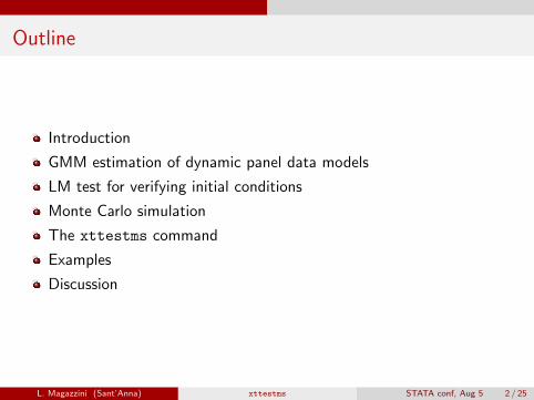
Introduction
GMM estimation of dynamic panel data models
LM test for verifying initial conditions
Monte Carlo simulation
The xttestms command
Examples
Discussion
L. Magazzini (Sant’Anna) xttestms STATA conf, Aug 5 2 / 25
Introduction
Introduction
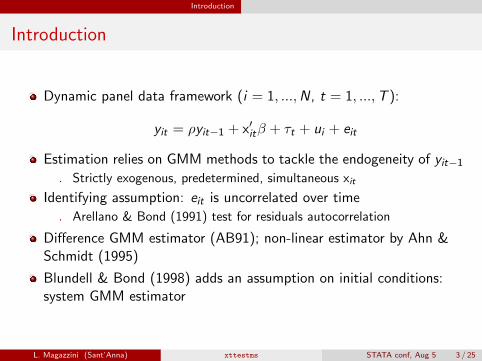
Dynamic panel data framework (i = 1, ...,N, t = 1, ...,T ):
yit = ρyit−1 + x′itβ + τt + ui + eit
Estimation relies on GMM methods to tackle the endogeneity of yit−1
. Strictly exogenous, predetermined, simultaneous xit
Identifying assumption: eit is uncorrelated over time
. Arellano & Bond (1991) test for residuals autocorrelation
Difference GMM estimator (AB91); non-linear estimator by Ahn &Schmidt (1995)
Blundell & Bond (1998) adds an assumption on initial conditions:system GMM estimator
L. Magazzini (Sant’Anna) xttestms STATA conf, Aug 5 3 / 25
GMM estimation
GMM estimationTo simplify, yit = ρyit−1 + ui + eit = ρyit−1 + εit
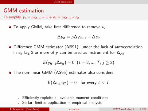
To apply GMM, take first difference to remove ui
∆yit = ρ∆yit−1 + ∆eit
Difference GMM estimator (AB91): under the lack of autocorrelationin eit lag 2 or more of y can be used as instrument for ∆yit
E (yit−j∆eit) = 0 (t = 2, ...,T ; j ≥ 2)
The non-linear GMM (AS95) estimator also considers
E (∆εitεiT ) = 0 for every t < T
. Efficiently exploits all available moment conditions
. So far, limited application in empirical analysis
L. Magazzini (Sant’Anna) xttestms STATA conf, Aug 5 4 / 25
GMM estimation
GMM estimationTo simplify, yit = ρyit−1 + ui + eit = ρyit−1 + εit
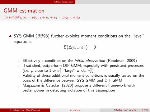
SYS GMM (BB98) further exploits moment conditions on the “level”equations:
E (∆yit−1εit) = 0
. Effectively a condition on the initial observation (Roodman, 2009)
. If satisfied, outperform DIF GMM, especially with persistent processes(i.e. ρ close to 1 or σ2
u “large” w.r.t. σ2e )
. Validity of these additional moment conditions is usually tested on thebasis of the difference between SYS GMM and DIF GMM
. Magazzini & Calzolari (2020) propose a different framework withbetter power in detecting violation of this assumption
L. Magazzini (Sant’Anna) xttestms STATA conf, Aug 5 5 / 25
LM test
The LM test for testing initial conditions(Magazzini & Calzolari, 2020)
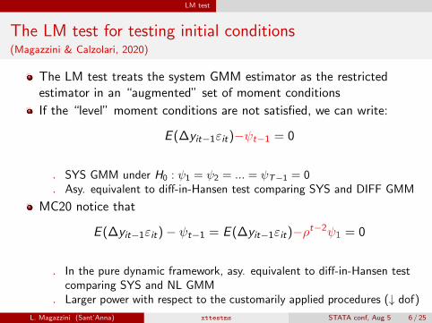
The LM test treats the system GMM estimator as the restrictedestimator in an “augmented” set of moment conditions
If the “level” moment conditions are not satisfied, we can write:
E (∆yit−1εit)−ψt−1 = 0
. SYS GMM under H0 : ψ1 = ψ2 = ... = ψT−1 = 0
. Asy. equivalent to diff-in-Hansen test comparing SYS and DIFF GMM
MC20 notice that
E (∆yit−1εit)− ψt−1 = E (∆yit−1εit)−ρt−2ψ1 = 0
. In the pure dynamic framework, asy. equivalent to diff-in-Hansen testcomparing SYS and NL GMM
. Larger power with respect to the customarily applied procedures (↓ dof)
L. Magazzini (Sant’Anna) xttestms STATA conf, Aug 5 6 / 25
LM test
The LM test for testing initial conditionsyit = ρyit−1 + x′itβ + εit
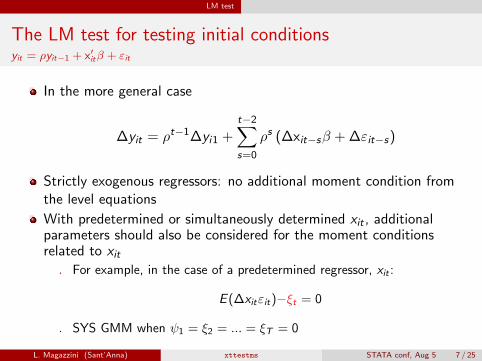
In the more general case
∆yit = ρt−1∆yi1 +t−2∑s=0
ρs (∆xit−sβ + ∆εit−s)
Strictly exogenous regressors: no additional moment condition fromthe level equations
With predetermined or simultaneously determined xit , additionalparameters should also be considered for the moment conditionsrelated to xit. For example, in the case of a predetermined regressor, xit :
E (∆xitεit)−ξt = 0
. SYS GMM when ψ1 = ξ2 = ... = ξT = 0
L. Magazzini (Sant’Anna) xttestms STATA conf, Aug 5 7 / 25
LM test
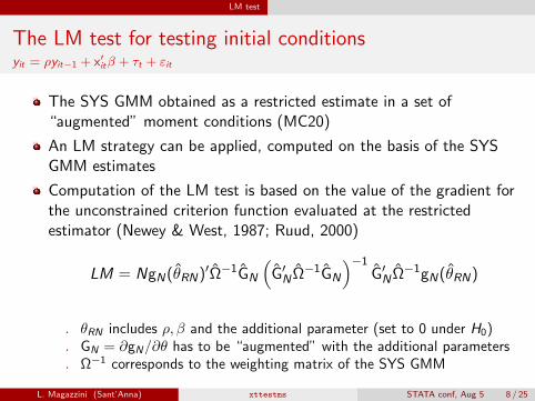
The LM test for testing initial conditionsyit = ρyit−1 + x′itβ + τt + εit
The SYS GMM obtained as a restricted estimate in a set of“augmented” moment conditions (MC20)
An LM strategy can be applied, computed on the basis of the SYSGMM estimates
Computation of the LM test is based on the value of the gradient forthe unconstrained criterion function evaluated at the restrictedestimator (Newey & West, 1987; Ruud, 2000)
LM = NgN(θRN)′Ω−1GN
(G′NΩ−1GN
)−1G′NΩ−1gN(θRN)
. θRN includes ρ, β and the additional parameter (set to 0 under H0)
. GN = ∂gN/∂θ has to be “augmented” with the additional parameters
. Ω−1 corresponds to the weighting matrix of the SYS GMM
L. Magazzini (Sant’Anna) xttestms STATA conf, Aug 5 8 / 25

Monte Carlo
Monte Carlo set up
yit = ρyit−1 + x′itβ + εit = ρyit−1 + x′itβ + ui + eit. ui ∼ N(0, σ2
u). eit = δiτtνit with δi ∼ U(0.5, 1.5), τt ∼ 0.5 + 0.1 t, and νit ∼ χ2
1 − 1(W05)
The regressor xit = ρx xit−1 + θuui + θeνit + wit
. θu = 0.25, θe = −0.1, wit ∼ N(0, 0.16) (BBW01)
. We set ρ = ρx = 0.5 and β = 1
. xit as strictly exogenous (νit ∼ N(0, 1)) or simultaneously determined(νit = eit)
Departure from mean stationarity by the parameters γy and γx thatmultiply the individual component in the initial observations
. Condition on initial observation satisfied if γy = γx = 1
L. Magazzini (Sant’Anna) xttestms STATA conf, Aug 5 9 / 25
Monte Carlo
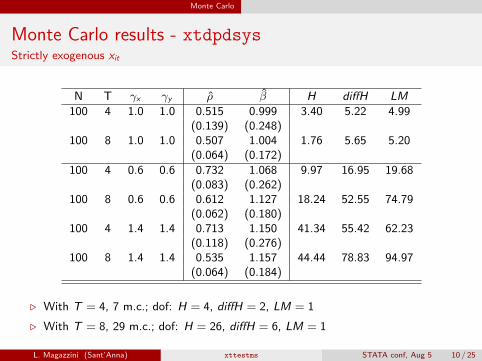
Monte Carlo results - xtdpdsysStrictly exogenous xit
N T γx γy ρ β H diffH LM
100 4 1.0 1.0 0.515 0.999 3.40 5.22 4.99(0.139) (0.248)
100 8 1.0 1.0 0.507 1.004 1.76 5.65 5.20(0.064) (0.172)
100 4 0.6 0.6 0.732 1.068 9.97 16.95 19.68(0.083) (0.262)
100 8 0.6 0.6 0.612 1.127 18.24 52.55 74.79(0.062) (0.180)
100 4 1.4 1.4 0.713 1.150 41.34 55.42 62.23(0.118) (0.276)
100 8 1.4 1.4 0.535 1.157 44.44 78.83 94.97(0.064) (0.184)
. With T = 4, 7 m.c.; dof: H = 4, diffH = 2, LM = 1
. With T = 8, 29 m.c.; dof: H = 26, diffH = 6, LM = 1
L. Magazzini (Sant’Anna) xttestms STATA conf, Aug 5 10 / 25
Monte Carlo
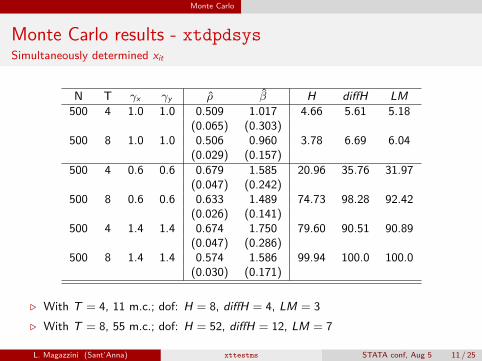
Monte Carlo results - xtdpdsysSimultaneously determined xit
N T γx γy ρ β H diffH LM
500 4 1.0 1.0 0.509 1.017 4.66 5.61 5.18(0.065) (0.303)
500 8 1.0 1.0 0.506 0.960 3.78 6.69 6.04(0.029) (0.157)
500 4 0.6 0.6 0.679 1.585 20.96 35.76 31.97(0.047) (0.242)
500 8 0.6 0.6 0.633 1.489 74.73 98.28 92.42(0.026) (0.141)
500 4 1.4 1.4 0.674 1.750 79.60 90.51 90.89(0.047) (0.286)
500 8 1.4 1.4 0.574 1.586 99.94 100.0 100.0(0.030) (0.171)
. With T = 4, 11 m.c.; dof: H = 8, diffH = 4, LM = 3
. With T = 8, 55 m.c.; dof: H = 52, diffH = 12, LM = 7
L. Magazzini (Sant’Anna) xttestms STATA conf, Aug 5 11 / 25
xttestms
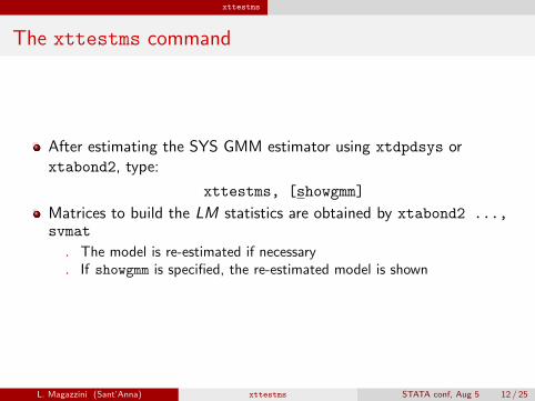
The xttestms command
After estimating the SYS GMM estimator using xtdpdsys orxtabond2, type:
xttestms, [showgmm]
Matrices to build the LM statistics are obtained by xtabond2 ...,svmat
. The model is re-estimated if necessary
. If showgmm is specified, the re-estimated model is shown
L. Magazzini (Sant’Anna) xttestms STATA conf, Aug 5 12 / 25

Examples
Example 1
Data used in Cameron and Trivedi (2005, ch. 21-22), taken fromZiliak (1997)
Labour supply of 532 individuals over the years 1979-1988
Dependent variable: lnhrs, the log of annual hours worked
Regressor: lnwg , the natural log of hourly wage
. Dynamic specification with no additional regressors
. lnwg as strictly exogenous, predetermined, simultaneously determined
L. Magazzini (Sant’Anna) xttestms STATA conf, Aug 5 13 / 25
Examples
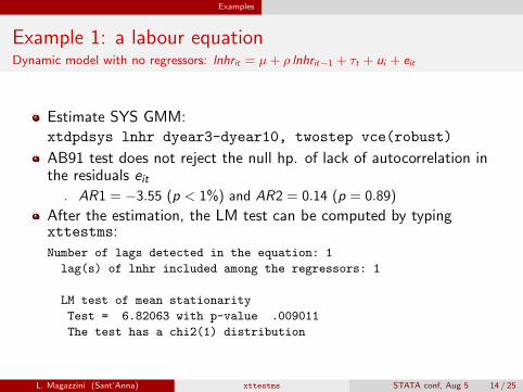
Example 1: a labour equationDynamic model with no regressors: lnhrit = µ+ ρ lnhrit−1 + τt + ui + eit
Estimate SYS GMM:xtdpdsys lnhr dyear3-dyear10, twostep vce(robust)
AB91 test does not reject the null hp. of lack of autocorrelation inthe residuals eit. AR1 = −3.55 (p < 1%) and AR2 = 0.14 (p = 0.89)
After the estimation, the LM test can be computed by typingxttestms:
Number of lags detected in the equation: 1
lag(s) of lnhr included among the regressors: 1
LM test of mean stationarity
Test = 6.82063 with p-value .009011
The test has a chi2(1) distribution
L. Magazzini (Sant’Anna) xttestms STATA conf, Aug 5 14 / 25

Examples
Example 1: dynamic model with no regressors“Augmented” m.c.: E(∆yit−1εit) − ρt−2ψ1 = 0
. mata: mata set matafavor speed
. xtabond2 lnhr l.lnhr dyear3-dyear10, gmmstyle(l.lnhr) h(2) ///
ivstyle(dyear3-dyear10, eq(level)) twostep robust svmat
...
. mat G=-(e(Z))’*(e(X))
. mat gpsi = J(colsof(e(Z),1,0)
. mat gpsi[colnumb(e(Z), "Levels eq:LD.lnhr/1981"),1]=-_b[L.lnhr]^0
. mat gpsi[colnumb(e(Z), "Levels eq:LD.lnhr/1982"),1]=-_b[L.lnhr]^1
. mat gpsi[colnumb(e(Z), "Levels eq:LD.lnhr/1983"),1]=-_b[L.lnhr]^2
...
. mat gpsi[colnumb(e(Z), "Levels eq:LD.lnhr/1988"),1]=-_b[L.lnhr]^7
. mat G=(G,gpsi)
. mat testcm = e(Ze)’*e(A2)*G*invsym(G’*e(A2)*G)*G’*e(A2)*e(Ze)
. Hansen test of overid. restrictions, equal to 68.26 with p-value 0.008
. Difference-in-Hansen test, equal to 16.22 with p-value 0.039
L. Magazzini (Sant’Anna) xttestms STATA conf, Aug 5 15 / 25
Examples
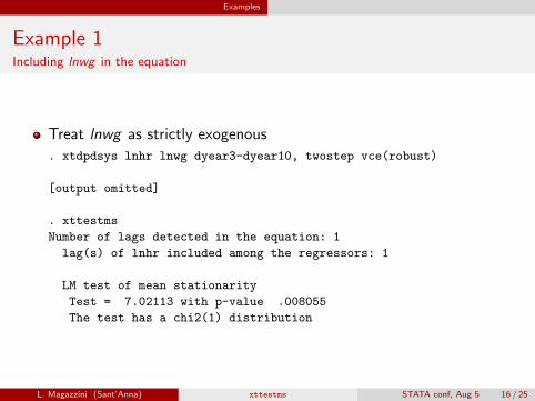
Example 1Including lnwg in the equation
Treat lnwg as strictly exogenous
. xtdpdsys lnhr lnwg dyear3-dyear10, twostep vce(robust)
[output omitted]
. xttestms
Number of lags detected in the equation: 1
lag(s) of lnhr included among the regressors: 1
LM test of mean stationarity
Test = 7.02113 with p-value .008055
The test has a chi2(1) distribution
L. Magazzini (Sant’Anna) xttestms STATA conf, Aug 5 16 / 25
Examples
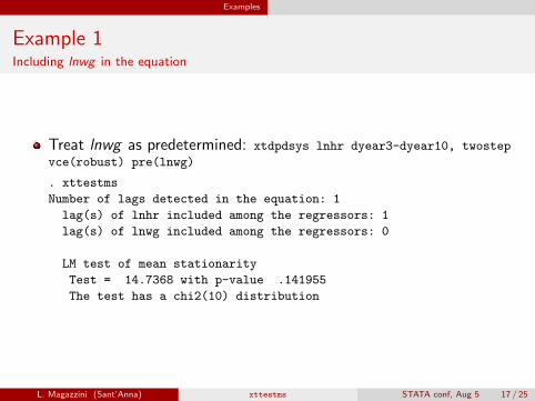
Example 1Including lnwg in the equation
Treat lnwg as predetermined: xtdpdsys lnhr dyear3-dyear10, twostep
vce(robust) pre(lnwg)
. xttestms
Number of lags detected in the equation: 1
lag(s) of lnhr included among the regressors: 1
lag(s) of lnwg included among the regressors: 0
LM test of mean stationarity
Test = 14.7368 with p-value .141955
The test has a chi2(10) distribution
L. Magazzini (Sant’Anna) xttestms STATA conf, Aug 5 17 / 25

Examples
Example 1Including lnwg in the equation
The test has 10 degrees of freedom as we are also considering the“augmented” moment conditions related to xit
E (∆xitεit)− ξt = 0
. By the recursive formula, these parameters also enter the m.c. relatedto yit−1
E (∆lnhri,80εi,81) = ψ1
E (∆lnhri,81εi,82) = E [(ρ∆lnhr80 + β∆lnwg81 + ∆e81)ε82]
= ρψ1 + βE (∆lnwg81ε82) = ρψ1 + βξ2
...
E (∆lnhri,87εi,88) = ρ7ψ1 + β(ρ6ξ2 + ρ5ξ3 + ...+ ξ8)
L. Magazzini (Sant’Anna) xttestms STATA conf, Aug 5 18 / 25
Examples
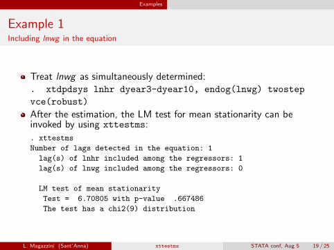
Example 1Including lnwg in the equation
Treat lnwg as simultaneously determined:. xtdpdsys lnhr dyear3-dyear10, endog(lnwg) twostep
vce(robust)
After the estimation, the LM test for mean stationarity can beinvoked by using xttestms:
. xttestms
Number of lags detected in the equation: 1
lag(s) of lnhr included among the regressors: 1
lag(s) of lnwg included among the regressors: 0
LM test of mean stationarity
Test = 6.70805 with p-value .667486
The test has a chi2(9) distribution
L. Magazzini (Sant’Anna) xttestms STATA conf, Aug 5 19 / 25

Examples
Example 2
usbal89.dta by Blundell & Bond (2000) and Bond (2002)
Balanced panel dataset of 509 US firms observed over 8 years,1982-1989
The estimated equation is. xi: xtabond2 y l.y n l.n k l.k i.year , ///gmm(y n k, lag(3 .)) iv(i.year, equation(level))twostep robust
. Only lags 3 or older can be used as legitimate instruments
. Lagged values of the regressors are included in the equation of interest
. Preferred specification: n and k as simultaneously determined
L. Magazzini (Sant’Anna) xttestms STATA conf, Aug 5 20 / 25
Examples
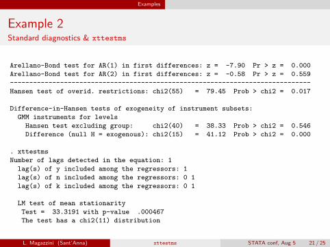
Example 2Standard diagnostics & xttestms
Arellano-Bond test for AR(1) in first differences: z = -7.90 Pr > z = 0.000
Arellano-Bond test for AR(2) in first differences: z = -0.58 Pr > z = 0.559
------------------------------------------------------------------------------
Hansen test of overid. restrictions: chi2(55) = 79.45 Prob > chi2 = 0.017
Difference-in-Hansen tests of exogeneity of instrument subsets:
GMM instruments for levels
Hansen test excluding group: chi2(40) = 38.33 Prob > chi2 = 0.546
Difference (null H = exogenous): chi2(15) = 41.12 Prob > chi2 = 0.000
. xttestms
Number of lags detected in the equation: 1
lag(s) of y included among the regressors: 1
lag(s) of n included among the regressors: 0 1
lag(s) of k included among the regressors: 0 1
LM test of mean stationarity
Test = 33.3191 with p-value .000467
The test has a chi2(11) distribution
L. Magazzini (Sant’Anna) xttestms STATA conf, Aug 5 21 / 25
Discussion
Discussion
LM test to better assess validity of initial condition in SYS GMM
Outperform customarily employed testing procedures
. In the pure dynamic case, the proposed procedure contrasts SYS andNL GMM
. Better performance in the case of strictly exogenous regressors
. Further work should consider alternative routes to detecting departuresfrom mean stationarity in the case of “endogenous” regressors
L. Magazzini (Sant’Anna) xttestms STATA conf, Aug 5 22 / 25

Discussion
Main references
AS95 Ahn, S.C. and Schmidt, P.: 1995, Efficient Estimation of Models for Dynamic Panel Data,Journal of Econometrics 68(1), 5–27
AB91 Arellano, M. and Bond, S.: 1991, Some Tests of Specification for Panel Data: MonteCarlo Evidence and an Application to Employment Equations, The Review of EconomicStudies 58(2), 277–297
BB98 Blundell, S. and Bond, S.: 1998, Initial Conditions and Moment Restrictions in DynamicPanel Data Models, Journal of Econometrics 87(1), 115–143
BB00 Blundell, S. and Bond, S.R.: 2000, GMM Estimation with Persistent Panel Data: anApplication to Production Functions, Econometric Reviews 19, 321–340
BBW01 Blundell, R., Bond, S. and Windmeijer, F.: 2001, Estimation in Dynamic Panel DataModels: Improving on the Performance of the Standard GMM Estimator, in Baltagi, B.H.,Fomby, T.B. and Hill, R.C. (eds.), Nonstationary Panels, Panel Cointegration, andDynamic Panels 15: 53–91, Emerald Group Publishing Ltd.
L. Magazzini (Sant’Anna) xttestms STATA conf, Aug 5 23 / 25
Discussion
Main references
B02 Bond, S.R.: 2002, Dynamic panel data models: A Guide to Micro Data Methods andPractice, Portuguese Economic Journal 1, 141–162
CT05 Cameron, A. C., and Trivedi, P. K.: 2005, Microeconometrics: Methods and Applications,Cambridge University Press.
MC20 Magazzini, L. and Calzolari, G.: 2020, Testing Initial Conditions in Dynamic Panel DataModels, Econometric Reviews 39(2), 115–134
NW87 Newey, W.K. and West, K.D.: 1987, Hypothesis Testing with Efficient Method ofMoment Estimation, International Economic Review 28, 777–787
R09 Roodman, D.: 2009, A Note on the Theme of Too Many Instruments, Oxford Bulletin ofEconomics and Statistics 71(1), 135–158
R00 Ruud, P.A. :2000, An Introduction to Classical Econometric Theory, Oxford UniversityPress
W05 Windmeijer, F.: 2005, A Finite Sample Correction for the Variance of Linear EfficientTwo-Step GMM Estimators, Journal of Econometrics 126(1), 25–51
Z97 Ziliak, J. P.: 1997, Efficient Estimation with Panel Data When Instruments arePredetermined: an Empirical Comparison of Moment-Condition Estimators, Journal ofBusiness & Economic Statistics 15(4), 419–431
L. Magazzini (Sant’Anna) xttestms STATA conf, Aug 5 24 / 25