Embed Size (px)
Citation preview
JOURNAL OF COMPUTATIONAL PHYSICS 37, l-18 (1980)
A Linear ADI Method for the Shallow-Water Equations
G.FAIRWEATHER
Deparrment of Mathematics, University of Kentucky, Lexington, Kentucky 40506
AND
I. M. NAVON
National Research Institute for Mathematical Sciences, CSIR, P.O. Box 395, Pretoria OaOl, South Africa
Received August 30, 1977; revised June 6, 1979
A new ADI method is proposed for the approximate solution of the shallow-water equa- tions. Based on a perturbation of a linearized Crank-Nicolson-type discretization, this method is algebraically linear and also locally second-order correct in time. Its performance on a test problem given in [ 11 demonstrates that it requires less computer time per time step than the fastest quasi-Newton method proposed in [ 1 1, and for given mesh parameters it appears to be marginally more accurate. The results of several long runs are also reported, and phenomena similar to those described in [ 141 are exhibited. In particular, it is shown that neither the new method nor the best of the methods of 111 conserves potential enstrophy and, as a result, after a finite time, these methods always “blow up.”
1. INTRODUCTION
To avoid the Courant-FriedrichsLevy (CFL) stability condition, restricting the time step in explicit finite-difference approximations to quasi-linear hyperbolic partial differential equations, implicit methods must be used. It is known [ 2, 3 ] that in hyper- bolic problems any dynamical degree of freedom that is stabilized by an implicit scheme in time, is treated inaccurately, viz., its phase speed is slowed down so that the explicit stability criteria are satisfied. On the other, hand, in meteorology, the high-speed oscillations which impose the severe upper limit on the time interval are unimportant, so that the deceleration of their phase speed poses no problem.
The numerical solution of nonlinear hyperbolic initial/boundary value problems in two space dimensions using an implicit method constitutes a formidable computational task. However, when the spatial region is rectangular this task can be simplified by using an alternating-direction implicit (ADI) method. Such methods reduce multidimensional problems to systems of one-dimensional problems [S, 8, 91. In this paper a new ADI method is proposed for the approximate solution of the
0021-9991/80/100001-189602.00/O CopyrIght t 1980 by Aoadcmx Press. In‘.
All rtghts of reproduction in any form rercrred
2 FAIRWEATHER AND NAVON
shallow-water equations, the primitive equations for an incompressible, inviscid fluid with a free surface, using the /?-plane approximation on a rectangular domain. Based on a perturbation of a linearized Crank-Nicolson-type discretization, this method is algebraically linear, that is, at each time step it requires the solution of systems of linear algebraic equations whereas the method of [ 1 ] involves systems of nonlinear equations. Like the method of [ 11, the new procedure is locally second-order correct in time.
An outline of the remainder of the paper is as follows. The differential equations and boundary conditions are given in Section 2. The salient features of Gustafsson’s method [ 1 ] are described in Section 3, and in Section 4 the new AD1 method is derived. In Section 5 the new method is tested on the same problem as that considered in [l] and using the same computer system (CDC 6600). It is shown that the new method requires less computer time per time step than the best of Gustafsson’s methods [ 11, QNEXl, and is marginally more accurate. The results of several long runs are of particular interest since they exhibit phenomena similar to those described in [ 141. In particular it is shown that neither the new method nor Gustafsson’s method, QNEXl, conserve potential enstrophy, and, as a result, after a certain time, which can be delayed by increasing the resolution, these methods “blow up.”
2. THE DIFFERENTIAL EQUATIONS AND BOUNDARY CONDITIONS
Throughout this paper we shall adopt the notation used in [ 11. We denote by w the vector function
w = (u, u, @)‘; (1)
where (w)’ denotes the transpose of w; U, 2, are the velocity components in the x and y directions, respectively; and
# = 2( g/z)“*,
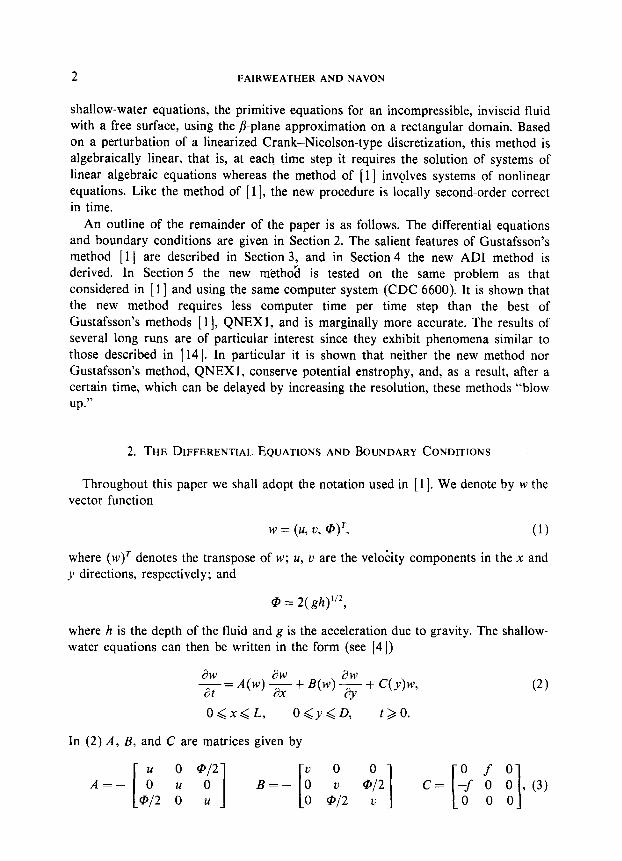
where h is the depth of the fluid and g is the acceleration due to gravity. The shallow- water equations can then be written in the form (see [4])
aW -= A(w) g + B(w) Jg + C(y)w, at
O<x<L, O<Y<D, t > 0.
In (2) A, B, and C are matrices given by
A=-[it ; ‘f] B=-[H j2 i2] c=
[
Of0 -f 0 0 0 00
(2)
I 9 (3)
LINEAR AD1 METHOD FOR SHALLOW-WATER EQUATIONS
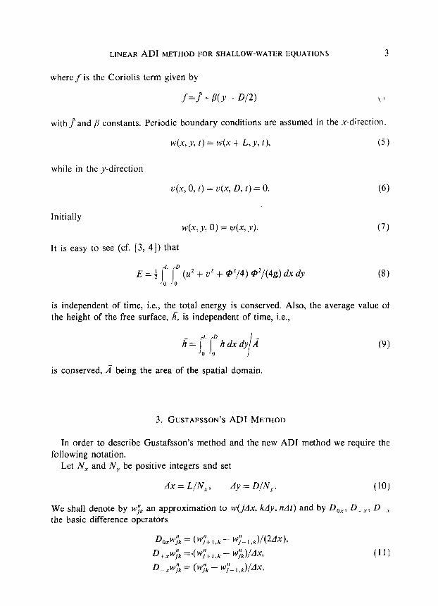
where f is the Coriolis term given by
.f=P+ NY - WI \‘:
with 3 and p constants. Periodic boundary conditions are assumed in the x-direction.
w(x, y, t) = w(x + L, y, t), (5)
while in the y-direction
u(x, 0, t) = u(x, D, t) = 0. (6)
Initially W(& YT 0) = w(4 Y)* (7)
It is easy to see (cf. 13, 41) that
E=; (u2 + u* + e/4) @‘/(4g) dx dy (8)
is independent of time, i.e., the total energy is conserved. Also, the average value of the height of the free surface, h; is independent of time, i.e.,
is conserved, A being the area of the spatial domain.
3. GUSTAFSSON’S AD1 METHOD
In order to describe Gustafsson’s method and the new AD1 method we require the following notation.
Let N, and N, be positive integers and set
Ax = L/N,, Ay = D/N,. (10)
We shall denote by w$ an approximation to w(jAx, kdy, ndt) and by DoX, D, X, D. .1 the basic difference operators
DoPi;, = <WY+ I ,/c - wi”- , .,)/(2,4x),
D+xwj”k =+‘;+ ,.k - w;&&
DLw$ = (wj;i - WY,,J/Ax,
(11)
4 FAIRWEATHER AND NAVON
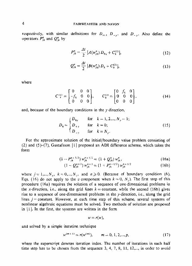
respectively, with similar definitions for Day , D,, , and D_,. Also define the operators P$ and Qyk by
where
(12)
(13)
(14)
and, because of the boundary conditions in the y-direction,
1 DO, for k = 1, 2,..., N, - 1;
D/c= D+, for k = 0; (15)
D-Y for k=N,.
For the approximate solution of the initial/boundary value problem consisting of (2) and (5)-(7), Gustafsson [ 1 ] proposed an ADI difference scheme, which takes the form
(1 - pi;: 1’2) wj:: Iv2 = (1 + Qjnk) w;~, (16a) (1 -Q,::‘)$+‘=(l +P;;1’2)w$.+“2 (16b)
where j = l,..., N,Y, k = 0 ,..,, N,,, and n > 0. (Because of boundary condition (6), Eqs. (16) do not apply to the u-component when k = 0, NY). The first step of this procedure (16a) requires the solution of a sequence of one-dimensional problems in the x-direction, i.e., along the grid lines k = constant, while the second (16b) gives rise to a sequence of one-dimensional problems in the y-direction, i.e., along the grid lines j = constant. However, at each time step of this scheme, several systems of nonlinear algebraic equations must be solved. Two methods of solution are proposed in [ 11. In the first, the systems are written in the form
w = r(w),
and solved by a simple iteration technique
W(m+ 1) = r(W(m)), m = 0, 1, 2 ,...) p, (17)
where the superscript denotes iteration index. The number of iterations in each half time step has to be chosen from the sequence 3, 4, 7, 8, 11, 12,..., in order to avoid
LLNEAR ADI METHOD FOR SHALLOW-WATER EQUATIONS 5
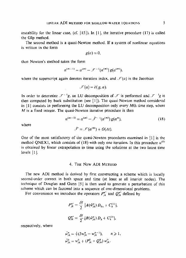
instability for the linear case, (cf. ] 151). In [ 11, the iterative procedure (17) is called the GIp method.
The second method is a quasi-Newton method. If a system of nonlinear equations is written in the form
g(a) = 0,
then Newton’s method takes the form
a(mt I) = a(m) - .P- ‘(a’“‘) g(cP)),
where the superscript again denotes iteration index, and .Y(a) is the Jacobian
X(a) = a( g, a).
In order to determine .P-‘g, an LU decomposition of ,P is performed and .P- ‘g is then computed by back substitution (see [ 1 I). The quasi-Newton method considered in [ 1 ] consists in performing the LU decomposition only every Mth time step, where M is a fixed integer. The quasi-Newton iterative procedure is then
a’mt 1) = a’m’ _ y-yaw) g(a”), (18) where
2 = f(aco’) + O(b).
One of the most satisfactory of the quasi-Newton procedures examined in [ 1 ] is the method QNEXl, which consists of (18) with only one iteration. In this procedure a”’
is obtained by linear extrapolation in time using the solutions at the two latest time levels [ 1 ].
4. THE NEW AD1 METHOD
The new AD1 method is derived by first constructing a scheme which is locally second-order correct in both space and time (at least at all interior nodes). The technique of Douglas and Gunn [5] is then used to generate a perturbation of this scheme which can be factored into a sequence of one-dimensional problems.
For convenience we introduce the operators P$ and Q$ defined by
Pi;: = $ [A($$) Do, + C:“],
respectively, where
6 FAIRWEATHER AND NAVON
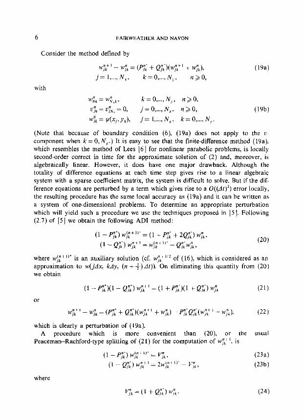
Consider the method defined by
wjk '+' - wTk = (I';; + Q$)(wj"k" + wyk),
j = 1 ,.. ., N, , k = 0 ,..., N, , n >o,
with
(194
Wn Ok = W;rkr k=O ,..., N,, n>O,
u,i”u = z&, = 0,
wyk = v(ij? Yk)r
j=O ,..., N,, n>O, (19b) j= l,..., N,, k= 0 ,..., N,.
(Note that because of boundary condition (6), (19a) does not apply to the u- component when k = 0, N,,.) It is easy to see that the finite-difference method (19a), which resembles the method of Lees [6] for nonlinear parabolic problems, is locally second-order correct in time for the approximate solution of (2) and, moreover, is algebraically linear. However, it does have one major drawback. Although the totality of difference equations at each time step gives rise to a linear algebraic system with a sparse coefficient matrix, the system is difficult to solve. But if the dif- ference equations are perturbed by a term which gives rise to a O((df)*) error locally, the resulting procedure has the same local accuracy as (19a) and it can be written as a system of one-dimensional problems. To determine an appropriate perturbation which will yield such a procedure we use the techniques proposed in [5]. Following (2.7) of [.5] we obtain the following AD1 method:
(l-pj”,‘)w;;+‘)‘= (1 + p;; + 2Q;;) w$, (1 -Q;;) w;;’ = ,j,+‘)* - Q,;w,“,, (20)
where w!““‘* is an auxiliary solution (cf. wyk+“* of (16), which is considered as an approximkation to w(jdx, kdy, (n + -f)dt)). On eliminating this quantity from (20) we obtain
(1 - P,$)( 1 - Q;;) wj:: ' = (1 + P,",')( 1 + Q,i",') w,;k (21)
or
wjk ’ + ’ - wik = (P;; + Q,n,‘)( wj:: ’ + wjnk) - I’;; Q,;; ( w,Jk+ ’ - wink), (22)
which is clearly a perturbation of (19a). A procedure which is more convenient than (20), or the usual
Peaceman-Rachford-type splitting of (21) for the computation of wyLt ‘. is
Pa)
Pb)
where
I’yk=(l +Q;;)wi;. (24)
LINEAR ADI METHOD FOR SHALLOW-WATER EQUATIONS 1
Upon eliminating w!” + ‘)’ between (23a) and (23b) we obtain Eq. (21) after some manipulation, Note ;Lat because of boundary condition (6) the Eqs. (23a) and (23b) do not apply to the u-component when k = 0, NY. In the following this new ADI method is called ADIF.
When system (2) is linear with time-independent coefficients, the new AD1 method (21) and Gustafsson’s method (16) (with r~i;:“* eliminated) are identical. Conse- quently the linear stability analysis given in [I ] for (16) also applies to (21).
Consider now the algebraic problem associated with ADIF, (23). Because of the form of the matrices A and B, no more than two variables are coupled to each other on the left-hand sides of the equations in (23). When the unknowns are ordered along horizontal rows for w(“+‘)‘, we first solve for the coupled variables (u$+ I)‘, Qj$‘+‘)‘), j= l,..., N,, k = O,..., N,, and only then for the variables uj,+ I)‘, j = I,..., N,, k = l,..., NY - 1. The elements of the vector w”‘+‘)’ are determined by solving for (u/$-t I”, @j;+ 1)‘) a sequence of linear systems whose coefficient matrices are cyclic block-tridiagonal matrices, each block being (2 X 2), and then solving for ujtt I)’ a sequence of linear systems whose coefficient matrices are scalar cyclic tridiagonal. The cyclic form of the tridiagonal matrices arises from the assumption of periodic boundary conditions in the x-direction. The scalar cyclic tridiagonal systems are solved using a routine from [ 131 which is based on the algorithm described in [7] while a generalization of the algorithm of [7] is used for the block cyclic tridiagonal systems.
When solving for wi;: ’ from (23b), the unknowns are ordered along vertical lines. The coupled variables (~7~’ i, @ykt ‘), k = 0 ,..., NY, j = l,..., N, are determined first, by solving block-tridiagonal systems using the subroutine BT of [IO]. The quantities u?“, k = 0 ,..., N,, j = 1 I..., N,, are then obtained by solving &terns using the standard routine; see, for example, [ 121.
scalar tridiagonal
5. NUMERICAL RESULTS
5.1. The Test Problem
To compare the computational efficiency and accuracy of the new AD1 method (23) with those of the method called QNEXI in [ 11, the test problem of [I] was used, viz., the initial height field condition No. 1 used by Grammeltvedt [ II]
h(x,J’)=H,,+H,tanh (““f;‘j) +H,sech2(9(D$-y)) sin(q. (25)
The initial velocity fields were derived from the initial height field via the geostrophic relationship
-g ah Id= f ay’ C--J -- (26)
8 FAIRWEATHER AND NAVON
The constants used were
L = 4400 km,
D = 6000 km,
3= 10m4 see-‘,
j3 = 1.5 X lo-” set-’ m-‘,
g = 10 msec-*,
Ho = 2000 m,
H, = 220 m,
H, = 133 m.
The time and space increments used in the short runs (2 days) were
(a) Ax = Ay = 200 km, At = 1800 set, (b) Ax = Ay = 200 km, At = 3600 sec.
For the long runs the space and time increments
Ax = Ay = 500 km, At = 3600 set,
were also used. All of the calculations were carried out on a CDC 6600 computer at the South
African Meteorological Offtce. Gustafsson’s experiments [l] were performed on a similar computer.
5.2. Computational Eflciency
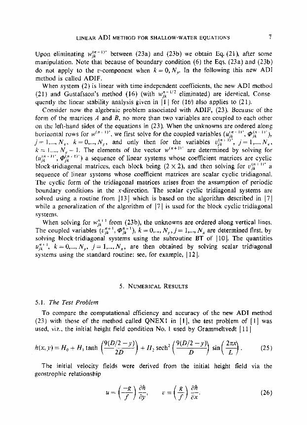
The methods QNEXl and ADIF were first compared by finding the run times in seconds per full time step. The results are shown in Table I, where OPT = 2 is an op- timized CDC version of FORTRAN, and OPT = 0 is a fast two-pass compilation with little optimization of object code. It is evident that ADIF is almost twice as fast as any of the versions of QNEXl of [ 11, a result which was not unexpected because, while the methods have similar operation counts ([ 115 + 152/M] NxlvY operations per full time step for QNEXl, 143N,N, for ADIF) QNEXl is more complicated to program than ADIF. Only the method G13 of [l] is faster than ADIF. However, the G13 method has a convergence criterion imposing a limit on A, = At/Ax, which is only four times as large as the CFL criterion for explicit schemes, and its convergence is very slow if A,, A, are near the convergence limit.
TABLE I
Method Run time
per full time step (set)
QNEXl, M = 12 0.43 QNEXl, M=6 0.49 ADIF (with OPT = 0) 0.25 ADIF (with OPT = 2) 0.23 G13 0.16
LINEAR AD1 METHOD FOR SHALLOW-WATER EQUATIONS 9
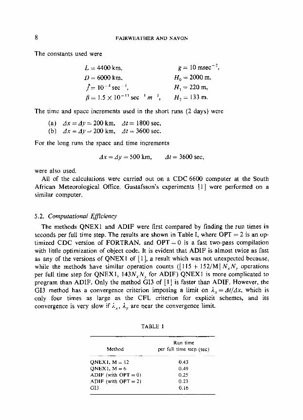
TABLE II
II ~ApllIII wEx II 0 = 2 days)
dx=dy=500km Ax = A,v = 200 km
Method Al = 3600 set At = 1800 set Af = 3600 set AI= 18OOsec
QNEXl (M= 6) 6..7 i x IO-’ 3.1 x lo-” 1.0x10 1 4.4 x 10 ADIF 5.4 1om4 2.3 10m4 8.7 x lo-’ 3.9 10 ( x x x
5.3. Accuracy
In order to provide a basis for comparison between the new method (ADIF) and Gustafsson’s QNEXl [ 11, we assume that the exact solution of the initial/boundary value problem (2), (5~(7), i+x, is the solution of (23) computed with a fine dis- cretization, viz., dx = dy = 50 km and At = 450 sec. As in [ 1 J, the relative error in an approximate solution, wAP, is measured in the norm (] . ]] defined by the inner product
where a and /I are grid functions satisfying the boundary conditions given in (19b). The relative errors in the approximations determined by QNEXl (M = 6) and ADIF are shown in Table II, where E,, = wAP - wEx.
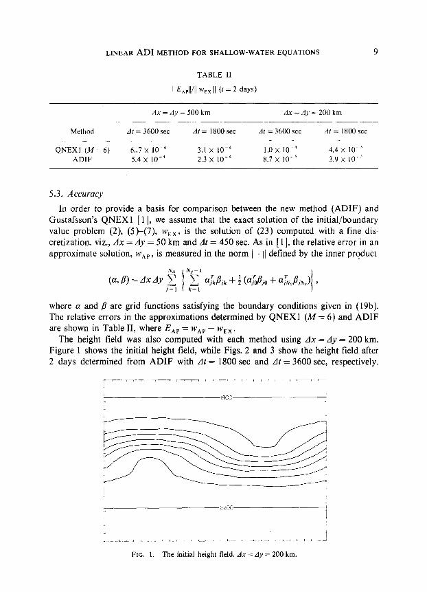
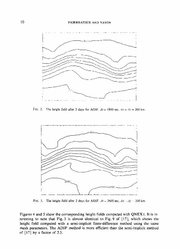
The height field was also computed with each method using Ax = Ay = 200 km. Figure 1 shows the initial height field, while Figs. 2 and 3 show the height field after 2 days determined from ADIF with At = 1800 set and At = 3600 set, respectively.
FIG. 1. The initial height field. dx = Ay = 200 km.
10 FAIRWEATHER AND NAVON
FIG. 2. The height field after 2 days for ADIF. df = 1800 sec. dx = dy = 200 km
FIG. 3. The height field after 2 days for ADIF. At = 3600 set, Ax = AJ = 200 km.
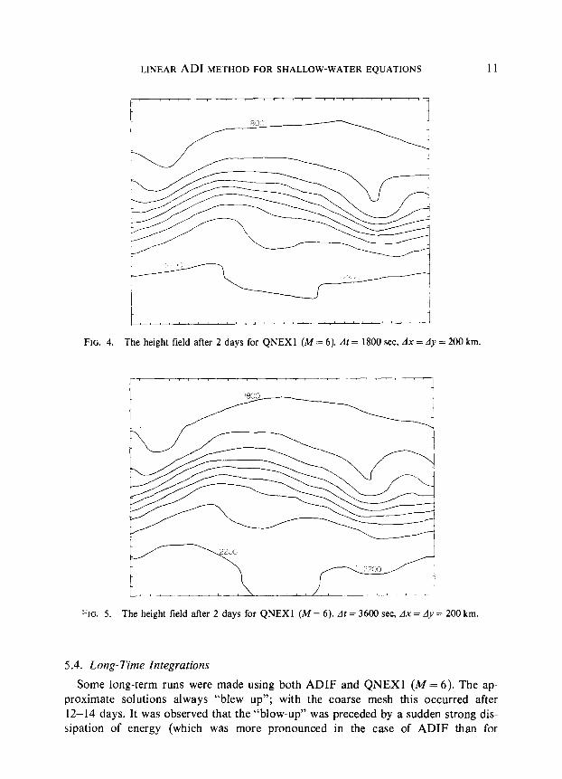
Figures 4 and 5 show the corresponding height fields computed with QNEX 1. It is in- teresting to note that Fig. 3 is almost identical to Fig. 9 of [ 171, which shows the height field computed with a semi-implicit finite-difference method using the same mesh parameters. The ADIF method is more efficient than the semi-implicit method of [ 171 by a factor of 2.5.
LINEAR ADI METHODFOR SHALLOW-WATEREQUATIONS 11
FIG. 4. The height field after 2 days for QNEXl (M = 6). At = 1800 set, Ax = Ay = 200 km.
r”“““““““” “““““‘I
“IG. 5. The height field after 2 days for QNEXl (M = 6). At = 3600 set, Ax = Ay = 200 km.
5.4. Long-Time Integrations
Some long-term runs were made using both ADIF and QNEXl (M= 6). The ap- proximate solutions always “blew up”; with the coarse mesh this occurred after 12-14 days. It was observed that the “blow-up” was preceded by a sudden strong dis- sipation of energy (which was more pronounced in the case of ADIF than for
12 FAIRWEATHER AND NAVON
QNEXl). This phenomenon appears to be a characteristic of energy-conserving models for the shallow-water equations. Sadourny [ 141 observed that for an energy- conserving model when this dissipation of energy occurs the potential enstrophy (the mean square potential vorticity) jumps by an order of magnitude. The potential enstrophy, Z, is a third invariant of the shallow-water equations, and is defined in the following way. If we denote by
I30 c
100
095
090
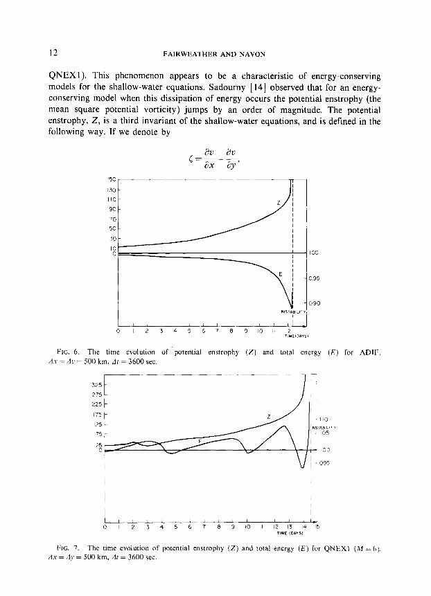
FIG. 6. The time evolution of .potential enstrophy (2) and total energy (E) for ADIF. A.u = AJ = 500 km. df = 3600 sec.
___---
I25 r 75 r
FIG. 7. The time evolution of potential enstrophy (2) and total energy (E) for QNEXl (M = 6). Ax=Ay=500 km, At= 3600sec.
LINEAR AD1 METHOD FOR SHALLOW-WATER EQUATIONS 13
the component of the relative vorticity along the local vertical, the absolute vorticity is defined as
Q=t+J Then
L L 2 z=: l^i‘ 0 0
$ dx dy.
Several numerical experiments were conducted to examine the time evolution of both the energy and the enstrophy invariants, E and Z, respectively, for the methods ADIF and QNEXl. Two spatial grids were used, namely,
and
Ax = Ay = 500 km, (27)
Ax = Ay =, 200 km, (28)
with At = 3600 set in each case. The results obtained from ADIF with (27) are plotted in Fig. 6. In this and subsequent figures the broken line denotes the “blow-up” time, T,. In this experiment the enstrophy increases linearly during the first 6 days, but in the vicinity of T, (~12 days) it jumps by an order of magnitude. The total energy remains reasonably constant for about 7 days after which it slowly decreases before decreasing sharply prior to “blow-up.” The discontinuity occurring at t = T, has been referred to as an “energy catastrophe” [ 141.
The results for QNEXl are given in Fig. 7. In this case T, is around 14 days and hence QNEXl is marginally more stable than ADIF. The behavior of E is quite different from that displayed in Fig. 6 but, again, a sharp decrease of E accompanied by a rapid increase in Z is observed prior to “blow-up.”
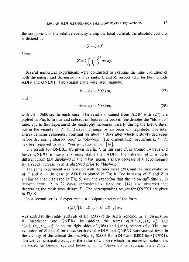
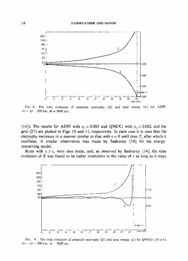
The same experiment was repeated with the finer mesh (28), and the time evolution of E and Z in the case of ADIF is plotted in Fig. 8. The behavior of E and Z is similar to that displayed in Fig. 6, with the exception that the “blow-up” time T, is delayed from 12 to 22 days, approximately. Sadourny [ 141 also observed that decreasing the mesh sizes delays T,. The corresponding results for QNEXl are given in Fig. 9.
In a second series of experiments a dissipation term of the form
was added to the right-hand side of Eq. (23a) of the ADIF scheme. In [ 1 ] dissipation is introduced into QNEXl by adding the terms &(At)‘l D,, De,, M$ and c(At)’ D+xDpxw;k+‘i2 to the right sides of (16a) and (16b), respectively. The time evolution of E and Z for these versions of ADIF and QNEXl was studied for E in the vicinity of the critical dissipativity, E, (0.003 for ADIF and 0.002 for QNEXl ). The critical dissipativity, E,, is the value of E above which the numerical solution is stabilized far beyond T,, and below which it “blows up” at approximately T, (cf.
14 FAIRWEATHER AND NAVON
260 -
220 -
180 -
140 -
100 -
60 - I
I , 1 I I
0 0 2 2 4 4 6 6 8 8 IO IO I2 I2 I4 14 16 16 18 18 20 20 22 22
1.00
095
090
ABILIT”
065
FIG. 8. The time evolution of potential enstrophy (Z) and total energy (E) for ADIF. AX = Ay = 200 km, dl= 36M) sec.
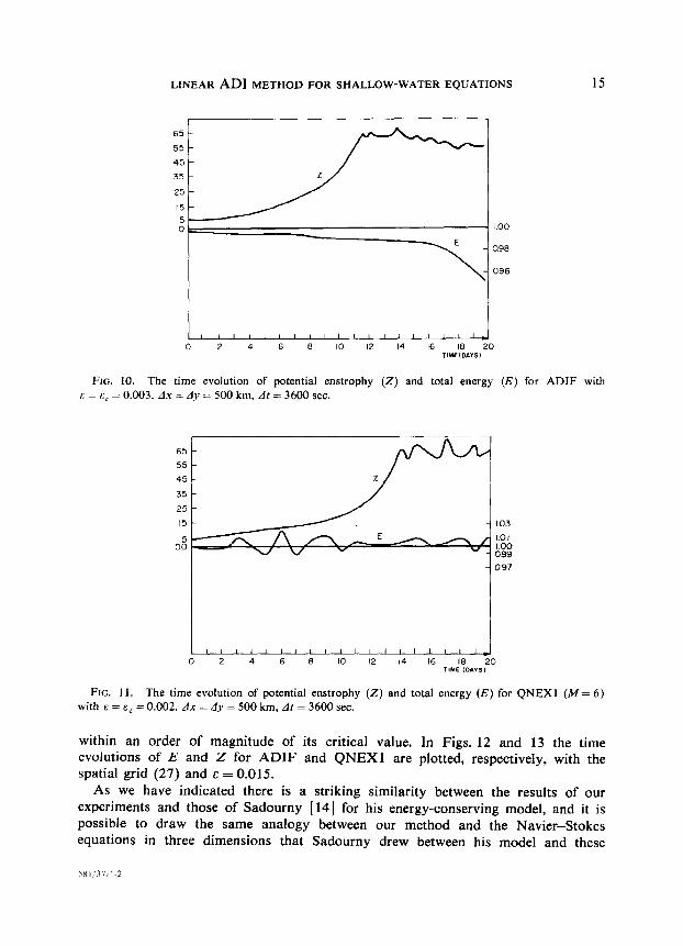
[ 14)). The results for ADIF with E, = 0.003 and QNEXl with E, = 0.002 and the grid (27) are plotted in Figs. 10 and 11, respectively. In each case it is seen that the enstrophy increases in a manner similar to that with E = 0 until time T, after which it oscillates. A similar observation was made by Sadourny [ 141 for his energy- conserving model.
Runs with E > E, were also made, and, as observed by Sadourny j14], the time evolution of E was found to be rather insensitive to the value of E as long as it stays
I I INSTABILIT”
IT 0 2 4 6 8 IO I2 I4 I6 I8 20 22 T’“~‘DA”51
FIG. 9. The time evolution of potential enstrophy (2) and total energy (E) for QNEX\ (M = 6) A.u=Ay= 200 km, At= 3600 sec.
LINEAR ADI METHOD FOR SHALLOW-WATER EQUATIONS 15
FIG. 10. The time evolution of potential enstrophy (2) and total energy E = E, = 0.003. Ax = Ay = 500 km, At = 3600 sec.
(I?) for ADIF with
0 2 4 6 8 IO 12 14 16 It3 20 TIME ,Dl"S,
FIG. 1 I. The time evolution of potential enstrophy (Z) and total energy (E) for QNEXl (M = 6) with E = E, = 0.002. Ax = Ay = 500 km, At = 3600 sec.
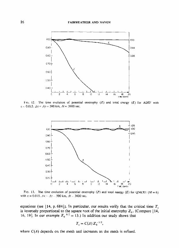
within an order of magnitude of its critical value. In Figs. 12 and 13 the time evolutions of E and Z for ADIF and QNEXl are plotted, respectively, with the spatial grid (27) and E = 0.015.
As we have indicated there is a striking similarity between the results of our experiments and those of Sadourny [ 141 for his energy-conserving model, and it is possible to draw the same analogy between our method and the Navier-Stokes equations in three dimensions that Sadourny drew between his model and these
16 FAIRWEATHER AND NAVON
100
099
098
060 -
050 -
040 -
0 2 4 6 8 IO 12 14 16 I8 20 TIME ,Dc%YIIs,
0 2 4 6 8 IO 12 14 I6 I8 20 TIME ,Dc%YIIs,
FIG. 12. The time evolution of potential enstrophy (2) and total energy (E) for ADIF with E = 0.015. Ax = dy = 500 km, AI = 3600 sec.
E E - I05 - I05
- 095 - 095
080 080 - -
070 070 - -
060 060 - -
050 050 - -
040 040 - -
030 030 - -
020 020 - - I I I I I I I I I 1 I I I I I I I I I I I 1 I I
0 0 2 2 4 4 6 6 8 8 IO IO I2 I2 I4 I4 I6 I6 I8 I8 20 20 TIME ,DP”S, TIME ,DP”S,
FIG. 13. The time evolution of potential enstrophy (Z) and total energy (E) for QNEXI (M = 6) with E = 0.015. Ax = AL’ = 500 km, At = 3600 sec.
equations (see [ 14, p. 6841). In particular, our results verify that the critical time T, is inversely proportional to the square root of the initial enstrophy Z,. (Compare [ 14, 16, 191. In our example Z; I” = 13.) In addition our study shows that
T, = C(d) Z, I”,
where C(d) depends on the mesh and increases as the mesh is refined,
LINEAR ADI METHODFORSHALLOW-WATEREQUATIONS 17
It should be emphasized that for the three-dimensional Navier-Stokes equations there exists an intrinsic critical time T,, independent of resolution. Since potential enstrophy is an invariant of the shallow-water equations, there is no intrinsic critical time for these equations. However, as observed by Sadourny [ 181, catastrophic behavior may occur at a finite time in numerical models if they do not conserve potential enstrophy. In this case the source of catastrophy lies in the truncation error and becomes less and less effective as resolution increases, and the critical time increases to infinity with resolution.
Finally, we emphasize a point made by Sadoumy. There is little to be gained by adding dissipation to ADIF and QNEXl. While dissipative terms stabilize the methods beyond T,, the catastrophe itself is unavoidable. Since the potential energy is an invariant of the shallow-water equations one should think of T, as the time beyond which the methods cease to be dynamically consistent with the original equa- tions, and consider calculations performed beyond that time as purely formal.
ACKNOWLEDGMENTS
Thanks are due to Mss J. Hewitt of NRIMS, CSIR, who did the programming. The work of the first author was partially supported by the National Science Foundation under Grant
MCS 75-0833 1.
REFERENCES
1. B. GUSTAFSSON, J. Comput. Physics 7 (1971), 239-254. 2. S. A. ORSZAG AND M. ISRAELI, Ann. Rev. Fluid Mech. (1974), 281-3 18. 3. M. KWIZAK, “Semi-implicit Integration of a Grid-Point Model of the Primitive Equations,” Depart-
ment of Meteorology, McGill University Publ. in Meteorology No. 98, 1970. 4. D. HOUGHTON, A. KASAHARA, AND W. WASHINGTON, Mon. Weather Rev. 94 (1966), 141-150. 5. J. DOUGLAS, JR., AND J. E. GUNN, Numer. Math. 6 (1964), 428-453. 6. M. LEES, in “Nonlinear Partial Differential Equations” (W. F. Ames, Ed.), pp. 193-201, Academic
Press, New York, 1967. 7. H. H. AHLBERG, E. N. NILSON, AND J. L. WALSH, “The Theory of Splines and Their Applications,”
Academic Press, New York, 1967. 8. N. N. YANENKO, “The Method of Fractional Steps,” Springer-Verlag, Berlin, 1971. 9. G. I. MARCHUK, “Numerical Methods in Weather Prediction,” Academic Press, New York, 1974.
10. A. C. HINDMARSH, “Solution of Block-TridiagonaJ Systems of Linear Algebraic Equations,” Lawrence Livermore Lab., UCID 30150, 1977.
11. A. GRAMMELTVEDT, Mon. Weather Rev. 97, No. 5 (1969), 384-404. 12. E. ISAACSON AND H. B. KELLER, “Analysis of Numerical Methods,” Wiley, New York, 1966. 13. I. M. NAVON. “Algorithms for the Solution of Scalar and Block Cyclic Tridiagonal Systems,” CSIR
Special Report WISK 265, Pretoria, South Africa, 1977. 14. R. SADOURNY, J. Atmos. Sci. 32 (1975), 68&689. 15. J. GARY, Math. Comput. 18 (1964), 1-18. 16. A. BRISSAUD, U. FRISCH, J. LEORAT, M. LESIEUR, A. MAZURE. A. POUQUE~. R. SADOURNY, AND P.
L. SULEM, Ann. Geophys. 29 (1973). 539-546.
18 FAIRWEATHER AND NAVON
17. 1. M. NAVON, Beit. Phys. Atmos. 51 (1978), 281-305. 18. R. SADOURNY, private communication. 19. C. BARDOS, in “Nonlinear Partial Differential Equations,” pp. l-46, Lecture Notes in Mathematics
No. 648, Springer-Verlag, New York, 1978.