Renewable Energy, Vol. 122, pp. 131-139, July 2018

Maira Bruck, Peter Sandborn, Navid Goudarzi The Center for Advanced Life Cycle Engineering (CALCE), Department of Mechanical Engineering, University of Maryland, Colelge Park, MD 20742, USA ABSTRACT

The cost of energy is a major concern for utilities, particularly for renewable energy, such as

wind, as consumers are sensitive to cost and renewable energy is typically more expensive than

conventional generation. Energy price and delivery risk are often balanced using Power Purchase

Agreements (PPAs). Since wind is not a constant supply source, in order to control risk, wind PPAs

contain clauses that require the purchase and sale of the energy to fall within prescribed limits. The

challenge addressed in this paper is that the price schedule in a PPA is determined using the

Levelized Cost of Energy (LCOE) provided by the Seller, but the energy delivery limits imposed

by the PPA impact the LCOE in ways that are not accommodated by existing LCOE models. This

paper develops a new cost model to evaluate the purchase price of electricity from a wind source

provided under a PPA contract and reveals that the actual LCOE under a PPA can be much higher

than the LCOE calculated using conventional means. It is critical for a PPA to have an appropriate

LCOE to ensure a “fair” energy purchase price. Sensitivity analysis demonstrates that PPA energy

purchase limitations can change the LCOE by as much as a factor of two depending. The

application of the model to real wind farms demonstrates that the actual LCOE depends on the

limitations on energy purchase within a PPA contract as well as the expected performance

characteristics associated with the wind farm. The new cost model can be used as a basis for setting

an appropriate PPA price schedule, thereby creating a method that the Seller can use to negotiate

penalties and an appropriate price for energy within their PPAs.

A Levelized Cost of Energy (LCOE) Model for Wind Farms that Include Power Purchase Agreements (PPAs)

2

KEYWORDS

Levelized Cost of Energy (LCOE), Power Purchase Agreements (PPAs), Wind Farms, Cost Model

NOMENCLATURE

CBI – Capacity-based incentive

CF – Capacity factor

CfD – Contract-for-Differences

COE – Cost of energy

CPE – Cost to produce energy

CRF – Capital recovery factor

D – Depreciation

E – Quantity of generated energy

EIA – U.S. Energy Information Administration

F – Fuel cost

I – Initial investment

IBI – Investment-based incentive

ITC – Investment tax credit

LCOE – Levelized cost of energy

Maxlim – Threshold for maximum energy delivery penalty (fraction)

Minlim – Threshold for minimum energy delivery penalty (fraction)

n – Number of years the LCOE applies

N – Number of turbines in the farm

NREL – National Renewable Energy Laboratory

3

O&M – Operation and maintenance

OM – Operation and maintenance cost

OREC – Offshore Renewable Energy Credit

Pexp – Annual expected power production

PPAterm – Fraction of the COE paid for energy above the maximum energy delivery limit

PBC – Performance-based contract

PBI – Production-based incentive

Pen – Total penalty cost

PL – Production loss

PN – Minimum penalty cost

PPA – Power Purchase Agreement

PTC – Production tax credit

PVOM – Present value of operation and maintenance costs

r – Weighted average cost of capital (discount rate)

R – Royalties or land rents

RP – Rated power

SAM – System Advisor Model

T – Tax levy

TC – Tax credit

TLCC – Total life-cycle cost

INTRODUCTION

Cost of Energy (COE) becomes a major concern for the public and utilities as the demand for

power from renewable energy sources, such as wind, increases. Utilities may become reluctant to

4

purchase more renewable energy than they are required to purchase if the COE is too high. COE

is the actual cost to buy energy while Levelized Cost of Energy (LCOE) is the break-even cost to

generate the energy. The LCOE is a commonly accepted calculation of the Total Life-Cycle Cost

(TLCC) for each unit of energy produced in the lifetime of a project[1].

In addition to the increase in the use of renewable energy sources, there is an increase in the

use of Power Purchase Agreements (PPAs) for all sources of energy. PPAs are Performance-Based

Contracts (PBCs) that aim to create a “fair” and risk-controlled agreement for the purchase and

sale of energy between a utility (the Buyer) and a generator (the Seller). The use of PPAs has been

increasing around the world and they are commonly used in Europe, the U.S., and in Latin

America. In Germany alone, wind projects with PPAs totaled over 1.2 GW in capacity in 2013[2].

In a data set from Berkeley Lab with a total of 34,558 MW of capacity in 387 signed or planned

PPAs for 2016-2017[3]. Between 2008 and 2016, 650 MW of new capacity was signed in the U.S.

and in 2015 the use of PPAs in the U.S. grew to 1.6 GW[4]. In Latin America, the governments

typically award PPAs instead of private corporations or utilities. In 2014, the government of Peru

awarded PPAs to projects with a total of 232 MW of capacity[5]. Within the U.S., PPAs have gained

more prominence as State governments set Renewable Portfolio Standards (RPS). RPS laws

mandate the level of renewable energy that a State is expected to consume. Utilities must then

purchase renewable energy at the levels required by the RPS[6]. Because renewable energy is

typically more expensive than gas or coal (at the current time in the U.S.), utilities will utilize a

maximum energy purchase limit so they do not have to purchase more of the expensive renewable

energy than required. In other parts of the world minimum energy purchase limits may be preferred

to maximum due to energy policies, as is the case in some Latin American countries. Government

policies shape the preferences to using a minimum, maximum, minimum and maximum, or no

5

energy purchase limitation in PPAs. Even within regions, such as Europe or Latin America,

because each country has different energy or environmental policies, energy purchase limitation

preferences vary. However, the basic concept of a PPA does not change between countries.

PPAs use an LCOE calculation to determine a fair price of energy, much like a standard retail

energy contract. However, Buyers in a PPA can create terms that limit the annual purchase of

energy, thereby affecting the actual LCOE. Buyers can create a limit for the minimum annual

amount of energy that needs to be delivered and/or the maximum amount that energy will be

bought at full price. The PPA contract limits create penalties; a penalty is incurred when the Seller

does not fall within the energy delivery requirements. In a normal energy contract (such as a

standard retail contract, a market retail contract, and in a PPA), the LCOE is calculated over the

period of the contract and energy is purchased as it arrives at the agreed upon point of delivery.

PPAs are used to share and reduce the risks of additional costs, however, in some cases the costs

are not accounted for within LCOE models. The term cost refers to a flow of money, while the

term risk refers to the combination of uncertainty in generation and transmission, and the cost

consequences that it carries. Electricity and PPA price are defined as the value energy is purchased

at. The exact risks managed by PPAs differ depending on the country and market the energy is sold

into. In a PPA, the risk of additional costs is negotiated between the Buyer and Seller. By taking

on more risk, the Buyer reduces the LCOE of the wind farm by taking on extra costs. In doing so,

the PPA price is reduced as the PPA price is negotiated around the actual LCOE of the wind farm.

A PPA is used to allocate risk between the Seller and the Buyer; additional costs to the Buyer that

arise from the allocated risks are reflected in the energy purchase limits as well as the PPA price.

The risks that are allocated to the Buyer reduce the LCOE of the wind farm because the Buyer

6

accepts the risk of those costs. Additional costs to the Buyer outside of the terms of the PPA do not

affect the LCOE of the wind farm.

Conventional LCOE models look at all the capital costs and annual operational costs that are

expected to be incurred in an energy project. PPAs address the capital costs, operational costs over

the lifetime of the project, the energy produced, tax credits, and the weighted average cost of capital

(WACC) within a specific project. The National Renewable Energy Laboratory (NREL) and others

have developed and used LCOE models that typically consider all or most of these parameters[7]-

[12]. The terms of the PPA are important because they create costs that affect the actual LCOE.

However, current LCOE models do not include the effects of the energy delivery limits and their

penalty costs imposed by PPAs as a cost to the wind farms. If the LCOE does not reflect the break-

even cost, the Seller risks the project’s failure and the Buyer risks a loss in profit from not

providing enough energy to its end-use consumers. A more accurate LCOE could prevent the

failure of a wind farm and benefit the Seller, the Buyer, and consumers.

In this paper, a new LCOE model is proposed to address the PPA annual energy delivery limits,

which we refer to as penalties. Although the application of penalties as a cost appears to be

straightforward (because of their direct and indirect costs to the Seller), the penalties are more

complex to analyze when uncertainties are introduced. The difference between the LCOE with

and without penalties can be significant (see the Wind Farm Case Study later in this paper). The

effect of penalties on the LCOE can vary depending on the capacity factor (CF), as well as the

limits on the purchase of energy. Determining the best limits in a PPA depends on the needs

(including governmental mandates) of the Buyer in conjunction with a desire for a COE that

reflects the actual LCOE for the Seller within the contract.

7

POWER PURCHASE AGREEMENTS (PPAS) AND LEVELIZED COST OF ENERGY

(LCOE)

PPAs can define every aspect of the project including: the terms for the entire project’s

construction, operation and maintenance (O&M), insurance, the interconnection and grid,

government involvement in the project, the delivery of energy, and any other third party

involvement in the project[13]. Each of these aspects is a responsibility of the Seller that affects the

cost of the wind farm. Normally, PPAs are viewed as just the relationship between the utility

(Buyer) and the generator (Seller), however, this paper views the PPA as a plan with specific

features defined for the success of the wind farm and all the parties involved.

During the negotiation of the PPA, the length of the agreement, the PPA price and the price

schedule are determined[14]. All the costs determined during negotiations are reviewed to calculate

the LCOE for the whole project and then the LCOE is used to determine a fair value for each unit

of energy produced. The negotiation of the COE and PPA terms is iterated until both parties are

satisfied. If the COE is too high, the terms are negotiated to drop the cost and if the terms create

extra costs, the COE is negotiated to a higher value.1 Although the PPA attempts to cover all the

costs in the contract, conventional LCOE models do not consider the penalties on annual energy

delivery limits as a cost. The purpose of creating annual energy delivery requirements is to be fair

to the Buyer who takes on the risk that the Seller will not be able to produce the required amount

of energy and the Buyer will then not be able to meet energy demand from the end-use customers.

The Buyer may not want to buy more expensive and unpredictable renewable energy, but may be

required to buy the energy by renewable energy requirements set by the government. This leads

1 For example, during a PPA negotiation, the risk of turbine failure may be mitigated by the Buyer creating

standards for how frequently Operations and Maintenance (O&M) should occur. The increase in O&M frequency increases the cost to the farm and thereby increases the estimated LCOE, in which case the COE in the contract would also increase.

8

the Buyer to create limits on the amount of energy they are willing to purchase. However, the costs

associated with these penalties are also a risk that could increase the LCOE without increasing the

COE or the PPA price. Thus, causing a loss in profit for the Seller. The effect of penalties must be

considered within the LCOE to ensure the fairness in (and the success of) the contract.

In some cases, PPAs create minimum energy delivery requirements[6]. If there is not enough

energy being provided by the Seller, then the Buyer has to look for energy elsewhere at, possibly,

spot-market prices. Spot-market prices vary hourly due to changing demand for energy – buying

and selling energy on the spot market is a risk that neither the Buyer nor the Seller wish to be

exposed to. The Buyer creates the minimum energy delivery requirement to reduce their risk and

the Seller has to pay at the PPA COE for every unit of energy under-delivered. Not all PPAs have

minimum energy requirements and some that have a minimum requirement also have a maximum

energy delivery requirement[15]. The maximum energy delivery requirement has been commonly

used in locations that have renewable energy requirements mandated by customers or the

government (and the Buyers would not otherwise purchase energy from renewable sources due to

higher prices, e.g., in the United States at the present time). Within a PPA, there are three different

requirements the Buyer can establish once the Seller has delivered the maximum energy delivery

limit before the end of the contracted period. The Buyer could require that the energy generated

cannot be further purchased by the Buyer or sold to another party, the energy could be purchased

at a fraction of the COE, or the energy could be sold in the spot-market. Both the spot-market and

wind energy production are unpredictable. Energy could be produced during a period of very low

demand and as such low spot-market prices would apply (e.g., at a faction of the LCOE).

Although wind farms produce energy that is bought and paid for monthly, the actual revenue

is calculated at the end of the year. At the end of each year, the Seller’s account is reviewed for

9

penalty costs and the over-purchase of energy to rectify the account balance. It is important to note

that the LCOE model needs to review the annual CF and not the monthly CF and energy generation

to determine the actual LCOE of a wind farm due to the PPA billing conditions described above.2

LEVELIZED COST OF ENERGY (LCOE)

The levelized cost of energy, also known the levelized cost of electricity, or the levelized energy

cost, is an economic assessment of the average total cost to build and operate a power-generating

system over its lifetime divided by the total power generated of the system over that lifetime[1].

The definition of LCOE is the cost that, if assigned to every unit of energy produced by the

system over the analysis period, will equal the Total Life-Cycle Cost (TLCC) when discounted

back to the base year[1],

∑ (1)

where discrete compounding is assumed, Ei is the amount of energy produced in year i, r is the

WACC (or discount rate), and n is the number of years over which the LCOE is calculated. E in

year i is the product of the rated power (RP) and the average capacity factor (CF) in year i. The

TLCC is the sum of the initial investment (I), and the present value of the total O&M costs (PVOM)

given by[1],

∑ (2)

2 This is always the case for wind farms because of the unpredictable nature of wind.

10

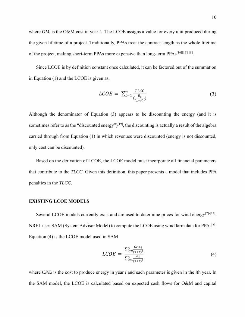
where OMi is the O&M cost in year i. The LCOE assigns a value for every unit produced during

the given lifetime of a project. Traditionally, PPAs treat the contract length as the whole lifetime

of the project, making short-term PPAs more expensive than long-term PPAs[16][17][18].

Since LCOE is by definition constant once calculated, it can be factored out of the summation

in Equation (1) and the LCOE is given as,

∑ 3

Although the denominator of Equation (3) appears to be discounting the energy (and it is

sometimes refer to as the “discounted energy”)[19], the discounting is actually a result of the algebra

carried through from Equation (1) in which revenues were discounted (energy is not discounted,

only cost can be discounted).

Based on the derivation of LCOE, the LCOE model must incorporate all financial parameters

that contribute to the TLCC. Given this definition, this paper presents a model that includes PPA

penalties in the TLCC.

EXISTING LCOE MODELS

Several LCOE models currently exist and are used to determine prices for wind energy[7]-[12].

NREL uses SAM (System Advisor Model) to compute the LCOE using wind farm data for PPAs[8].

Equation (4) is the LCOE model used in SAM

∑

∑ (4)

where CPEi is the cost to produce energy in year i and each parameter is given in the ith year. In

the SAM model, the LCOE is calculated based on expected cash flows for O&M and capital

11

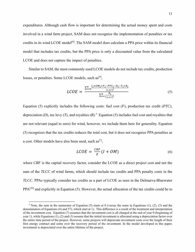
expenditures. Although cash flow is important for determining the actual money spent and costs

involved in a wind farm project, SAM does not recognize the implementation of penalties or tax

credits in its wind LCOE model[8]. The SAM model does calculate a PPA price within its financial

model that includes tax credits, but the PPA price is only a discounted value from the calculated

LCOE and does not capture the impact of penalties.

Similar to SAM, the most commonly used LCOE models do not include tax credits, production

losses, or penalties. Some LCOE models, such as[9],

∑

∑ (5)

Equation (5) explicitly includes the following costs: fuel cost (F), production tax credit (PTC),

depreciation (D), tax levy (T), and royalties (R).3 Equation (5) includes fuel cost and royalties that

are not relevant (equal to zero) for wind, however, we include them here for generality. Equation

(5) recognizes that the tax credits reduces the total cost, but it does not recognize PPA penalties as

a cost. Other models have also been used, such as[7],

(6)

where CRF is the capital recovery factor, consider the LCOE as a direct project cost and not the

sum of the TLCC of wind farms, which should include tax credits and PPA penalty costs in the

TLCC. PPAs typically consider tax credits as a part of LCOE as seen in the Delmarva-Bluewater

PPA[20] and explicitly in Equation (5). However, the actual allocation of the tax credits could be to

3 Note, the sum in the numerator of Equation (5) starts at 0 (versus the sums in Equations (1), (2), (3) and the

denominators of Equations (4) and 57), which start at 1). This difference is a result of the treatment and interpretation of the investment cost. Equation (7) assumes that the investment cost is all charged at the end of year 0 (beginning of year 1), while Equations (1), (2) and (3) assume that the initial investment is allocated using a depreciation factor over the entire time period of the project. However, some projects will depreciate investment costs over the length of their first energy contract and some over the recovery period of the investment. In the model developed in this paper, investment is depreciated over the entire lifetime of the project.

12

any party. Tax credits are a mechanism used to reduce the cost of producing energy, specifically in

the cases of renewable energy. In the case of renewable energy, tax credits to reduce the LCOE by

creating another source of revenue, thus allowing them to compete in the market against other

energy sources such as coal and oil. The extra revenue generated by tax credits is included in the

LCOE equation and is then incorporated into the PPA price. While tax credits are included in the

LCOE equation as a reduction to the LCOE, the LCOE calculation does not consider the additional

cost of penalties in the total life-cycle cost.

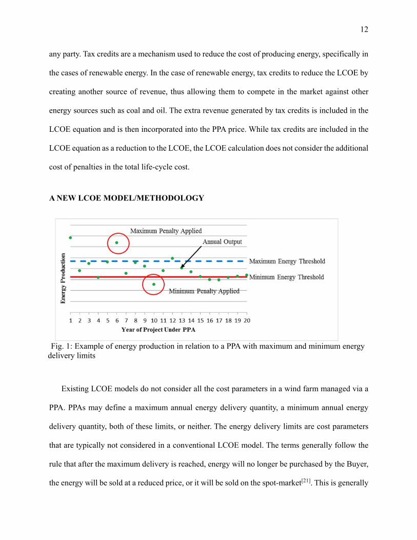
A NEW LCOE MODEL/METHODOLOGY

Existing LCOE models do not consider all the cost parameters in a wind farm managed via a

PPA. PPAs may define a maximum annual energy delivery quantity, a minimum annual energy

delivery quantity, both of these limits, or neither. The energy delivery limits are cost parameters

that are typically not considered in a conventional LCOE model. The terms generally follow the

rule that after the maximum delivery is reached, energy will no longer be purchased by the Buyer,

the energy will be sold at a reduced price, or it will be sold on the spot-market[21]. This is generally

Fig. 1: Example of energy production in relation to a PPA with maximum and minimum energy

delivery limits

13

considered a cost/penalty for the Seller since they lose some value of the energy that is produced

after the maximum delivery quantity is reached. Similarly, there is a direct cost/penalty in the

minimum energy delivery defined in the PPA, as every unit of under-produced energy must be paid

back at the agreed upon COE. The PacifiCorp draft PPA is an example PPA with a minimum energy

delivery penalty, which is referred to as the liquidated damages from output shortfall in the PPA[22].

In Fig. 1, the maximum and minimum energy limits demonstrate how the penalties are applied.

Each year that the energy production is above or below the limits as shown in Fig. 1, the penalty

is applied. The new model reflects the costs of energy production that is above the maximum or

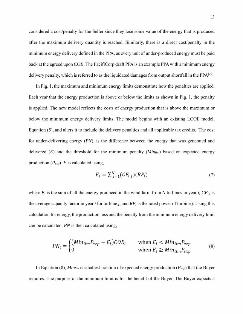
below the minimum energy delivery limits. The model begins with an existing LCOE model,

Equation (5), and alters it to include the delivery penalties and all applicable tax credits. The cost

for under-delivering energy (PN), is the difference between the energy that was generated and

delivered (E) and the threshold for the minimum penalty (Minlim) based on expected energy

production (Pexp). E is calculated using,

∑ , (7)

where Ei is the sum of all the energy produced in the wind farm from N turbines in year i, CFi,j is

the average capacity factor in year i for turbine j, and RPj is the rated power of turbine j. Using this

calculation for energy, the production loss and the penalty from the minimum energy delivery limit

can be calculated. PN is then calculated using,

when

0when (8)

In Equation (8), Minlim is smallest fraction of expected energy production (Pexp) that the Buyer

requires. The purpose of the minimum limit is for the benefit of the Buyer. The Buyer expects a

14

minimum amount of energy to meet the demands of its consumers. If the energy does not meet the

requirement, then the Buyer has to go to an outside source (e.g., the spot-market) and may have to

purchase energy at a higher price, which the Buyer will require the Seller to compensate them for.

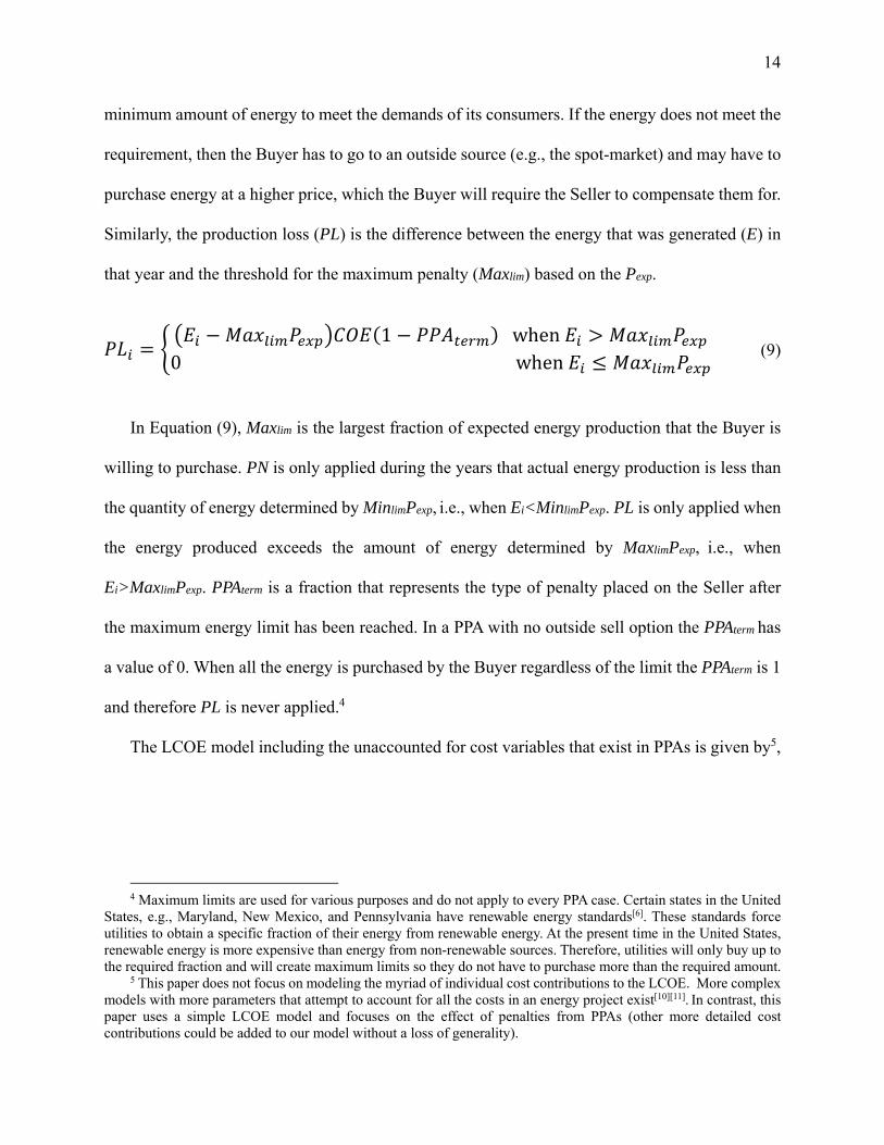
Similarly, the production loss (PL) is the difference between the energy that was generated (E) in

that year and the threshold for the maximum penalty (Maxlim) based on the Pexp.

1 when0when

(9)

In Equation (9), Maxlim is the largest fraction of expected energy production that the Buyer is

willing to purchase. PN is only applied during the years that actual energy production is less than

the quantity of energy determined by MinlimPexp, i.e., when Ei<MinlimPexp. PL is only applied when

the energy produced exceeds the amount of energy determined by MaxlimPexp, i.e., when

Ei>MaxlimPexp. PPAterm is a fraction that represents the type of penalty placed on the Seller after

the maximum energy limit has been reached. In a PPA with no outside sell option the PPAterm has

a value of 0. When all the energy is purchased by the Buyer regardless of the limit the PPAterm is 1

and therefore PL is never applied.4

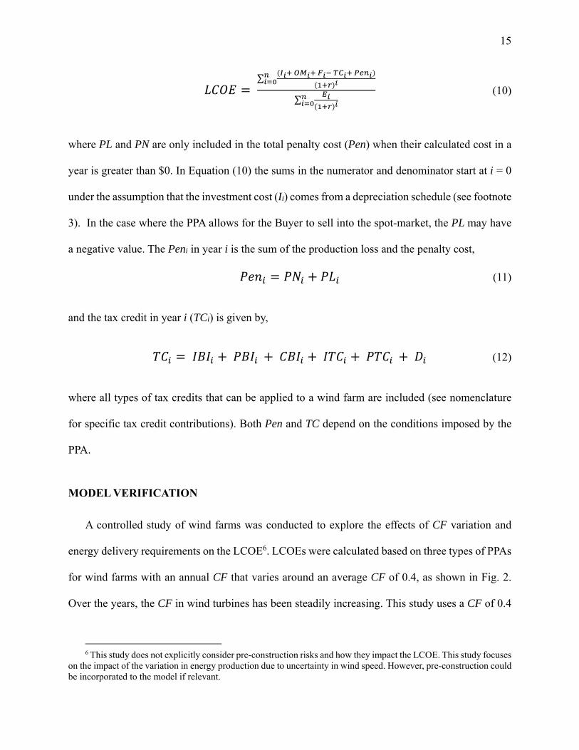
The LCOE model including the unaccounted for cost variables that exist in PPAs is given by5,

4 Maximum limits are used for various purposes and do not apply to every PPA case. Certain states in the United

States, e.g., Maryland, New Mexico, and Pennsylvania have renewable energy standards[6]. These standards force utilities to obtain a specific fraction of their energy from renewable energy. At the present time in the United States, renewable energy is more expensive than energy from non-renewable sources. Therefore, utilities will only buy up to the required fraction and will create maximum limits so they do not have to purchase more than the required amount.

5 This paper does not focus on modeling the myriad of individual cost contributions to the LCOE. More complex models with more parameters that attempt to account for all the costs in an energy project exist[10][11]. In contrast, this paper uses a simple LCOE model and focuses on the effect of penalties from PPAs (other more detailed cost contributions could be added to our model without a loss of generality).

15

∑

∑ (10)

where PL and PN are only included in the total penalty cost (Pen) when their calculated cost in a

year is greater than $0. In Equation (10) the sums in the numerator and denominator start at i = 0

under the assumption that the investment cost (Ii) comes from a depreciation schedule (see footnote

3). In the case where the PPA allows for the Buyer to sell into the spot-market, the PL may have

a negative value. The Peni in year i is the sum of the production loss and the penalty cost,

(11)

and the tax credit in year i (TCi) is given by,

(12)

where all types of tax credits that can be applied to a wind farm are included (see nomenclature

for specific tax credit contributions). Both Pen and TC depend on the conditions imposed by the

PPA.

MODEL VERIFICATION

A controlled study of wind farms was conducted to explore the effects of CF variation and

energy delivery requirements on the LCOE6. LCOEs were calculated based on three types of PPAs

for wind farms with an annual CF that varies around an average CF of 0.4, as shown in Fig. 2.

Over the years, the CF in wind turbines has been steadily increasing. This study uses a CF of 0.4

6 This study does not explicitly consider pre-construction risks and how they impact the LCOE. This study focuses

on the impact of the variation in energy production due to uncertainty in wind speed. However, pre-construction could be incorporated to the model if relevant.

16

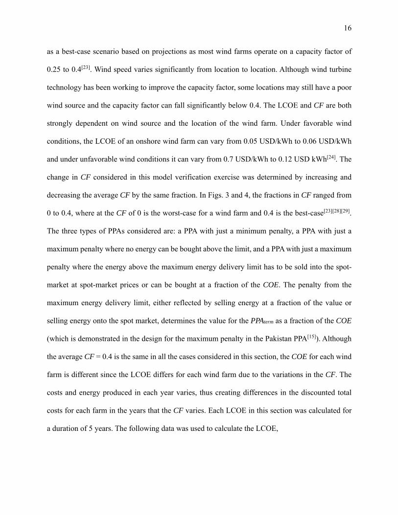
as a best-case scenario based on projections as most wind farms operate on a capacity factor of

0.25 to 0.4[23]. Wind speed varies significantly from location to location. Although wind turbine

technology has been working to improve the capacity factor, some locations may still have a poor

wind source and the capacity factor can fall significantly below 0.4. The LCOE and CF are both

strongly dependent on wind source and the location of the wind farm. Under favorable wind

conditions, the LCOE of an onshore wind farm can vary from 0.05 USD/kWh to 0.06 USD/kWh

and under unfavorable wind conditions it can vary from 0.7 USD/kWh to 0.12 USD kWh[24]. The

change in CF considered in this model verification exercise was determined by increasing and

decreasing the average CF by the same fraction. In Figs. 3 and 4, the fractions in CF ranged from

0 to 0.4, where at the CF of 0 is the worst-case for a wind farm and 0.4 is the best-case[23][28][29].

The three types of PPAs considered are: a PPA with just a minimum penalty, a PPA with just a

maximum penalty where no energy can be bought above the limit, and a PPA with just a maximum

penalty where the energy above the maximum energy delivery limit has to be sold into the spot-

market at spot-market prices or can be bought at a fraction of the COE. The penalty from the

maximum energy delivery limit, either reflected by selling energy at a fraction of the value or

selling energy onto the spot market, determines the value for the PPAterm as a fraction of the COE

(which is demonstrated in the design for the maximum penalty in the Pakistan PPA[15]). Although

the average CF = 0.4 is the same in all the cases considered in this section, the COE for each wind

farm is different since the LCOE differs for each wind farm due to the variations in the CF. The

costs and energy produced in each year varies, thus creating differences in the discounted total

costs for each farm in the years that the CF varies. Each LCOE in this section was calculated for

a duration of 5 years. The following data was used to calculate the LCOE,

17

I = $1500 per installed kW[25]

OM = $0.01 per kWh produced[25]

F = $0

TC = $0.05 per kWh sold[26]

r = 0.089 per year[27]

RP = 3000

COE = LCOE from Equation (12) with Peni = 0 and using Equation (7) for Ei

The investment (I), although shown as a single value, is a value that is depreciated over the

lifetime, or in many cases the length of the PPA, of the wind farm and changes for every year i.

The COE in a PPA is generally calculated from an LCOE that does not consider delivery penalties

as a cost. For this reason, the cost calculated from penalties in the new model uses the calculated

LCOE (for an individual wind farm) under a PPA without penalties as the COE. Pexp is calculated

as the average annual expected energy production from a specific farm. In these cases, the expected

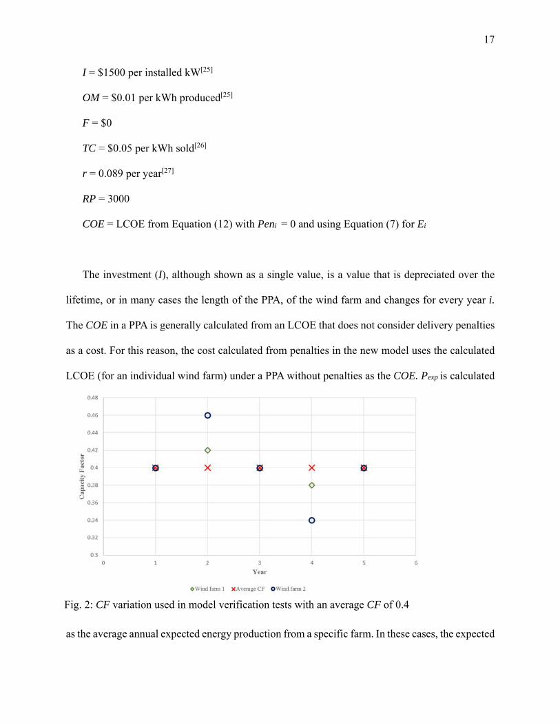
Fig. 2: CF variation used in model verification tests with an average CF of 0.4

18

energy production is calculated using a CF of 0.4 for every year (Danish wind farms averaged 0.41

in 2012[28] and it has been predicted that between 2005 and 2030, wind farms will be operating at

capacity factors between 0.36 and 0.43[29]). Ei is calculated using a CF that is based on the

variability around the average CF. The values of Minlim, Maxlim, and Ei, are then used to calculated

penalties.

CF variation in the following series of tests was generate as the fraction of energy that is

produced in year i that falls above or below the average CF of a project. Fig. 2 demonstrates this

with two farms that have an average CF of 0.4 over 5 years. Wind farm 1 in this case has a CF

variation of 0.05, this means that 0.05 more energy is produced in one year and 0.05 less is

produced in another. Wind farm 2 in Fig. 2 is similar as it assumes a CF variation of 0.15. The

algorithm used in this study valued year 2 as the higher than “expected” CF year and year 4 as the

lower than “expected” CF year. A different pattern of uncertainty than Fig. 2 would yield different

results. We only use the pattern in Fig. 2 as a simple example for model verification purposes (in

the case study in the next section of this paper we have used actual CFs for actual wind farms).

19

Fig. 3 shows the results for a PPA with only a minimum energy delivery limit. In this case, as

the variation in the CF increases, more energy is likely to fall below the annual minimum

requirement, thus increasing the LCOE. The greater the variation, the more likely the LCOE will

be affected by the minimum energy delivery limits. The domain for Minlim is [0,1], because the

required minimum annual delivery quantity could range from no required quantity, Minlim = 0, to

a requirement for the entire expected output of the wind farm, Minlim = 1. The increase in values

for the different variations in Fig. 3 are ramps where the LCOE increases between values of Minlim

and then increases at a slower rate thereafter. Before the value of Minlim where the LCOE starts to

increase, the LCOE has no dependence on Minlim, i.e., in these cases there is no energy produced

below Minlim. When there is no variation in the CF (the “None” case in Fig. 3), the LCOE is

independent of Minlim.

Fig. 3: Offshore PPA with just a minimum energy delivery limit with different variations in energy around the average CF = 0.4.

20

The value of Maxlim can range from 0 to greater than 1. Maxlim = 0 implies that every unit of

energy produced is penalized, and Maxlim = 1 implies that every unit of energy over Pexp (the annual

expected energy production) is penalized and every unit of energy below Pexp is not penalized.

However, a PPA will generally not create a Maxlim much lower than 0.5. The Maxlim may also

exceed 1 because of variation. If a wind farm generates above the expected energy production

every few years, a Maxlim greater than 1 gives the wind farm room to avoid being penalized for

producing more than Pexp.

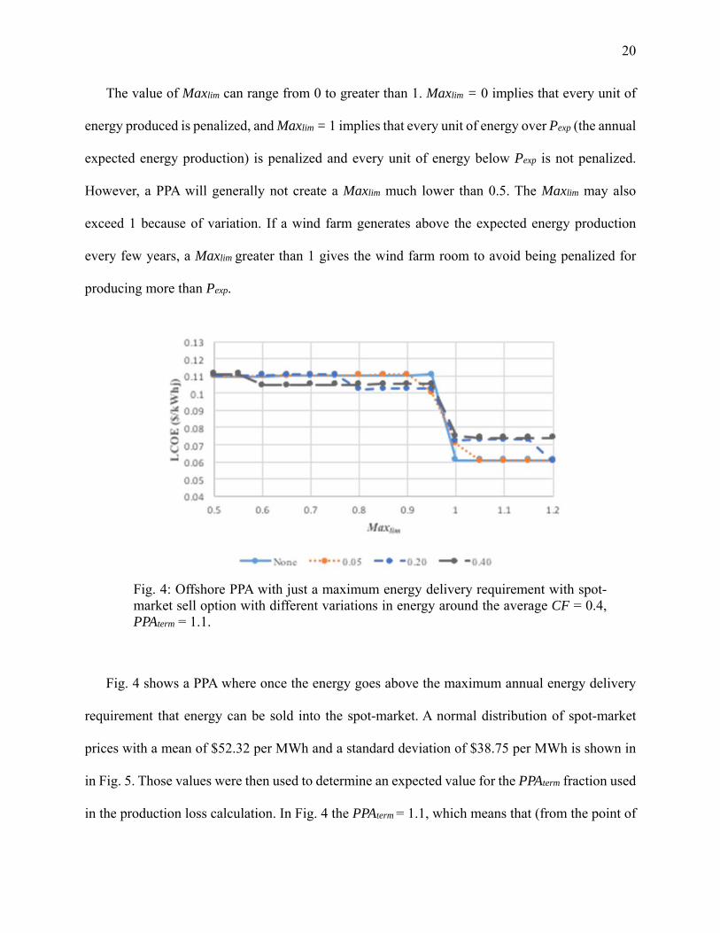
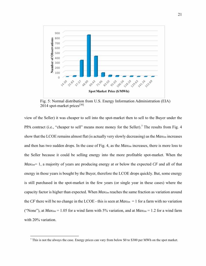
Fig. 4 shows a PPA where once the energy goes above the maximum annual energy delivery

requirement that energy can be sold into the spot-market. A normal distribution of spot-market

prices with a mean of $52.32 per MWh and a standard deviation of $38.75 per MWh is shown in

in Fig. 5. Those values were then used to determine an expected value for the PPAterm fraction used

in the production loss calculation. In Fig. 4 the PPAterm = 1.1, which means that (from the point of

Fig. 4: Offshore PPA with just a maximum energy delivery requirement with spot-market sell option with different variations in energy around the average CF = 0.4, PPAterm = 1.1.

21

view of the Seller) it was cheaper to sell into the spot-market then to sell to the Buyer under the

PPA contract (i.e., “cheaper to sell” means more money for the Seller).7 The results from Fig. 4

show that the LCOE remains almost flat (is actually very slowly decreasing) as the Maxlim increases

and then has two sudden drops. In the case of Fig. 4, as the Maxlim increases, there is more loss to

the Seller because it could be selling energy into the more profitable spot-market. When the

Maxlim= 1, a majority of years are producing energy at or below the expected CF and all of that

energy in those years is bought by the Buyer, therefore the LCOE drops quickly. But, some energy

is still purchased in the spot-market in the few years (or single year in these cases) where the

capacity factor is higher than expected. When Maxlim reaches the same fraction as variation around

the CF there will be no change in the LCOE - this is seen at Maxlim = 1 for a farm with no variation

(“None”), at Maxlim = 1.05 for a wind farm with 5% variation, and at Maxlim = 1.2 for a wind farm

with 20% variation.

7 This is not the always the case. Energy prices can vary from below $0 to $300 per MWh on the spot market.

Fig. 5: Normal distribution from U.S. Energy Information Administration (EIA) 2014 spot-market prices[30]

22

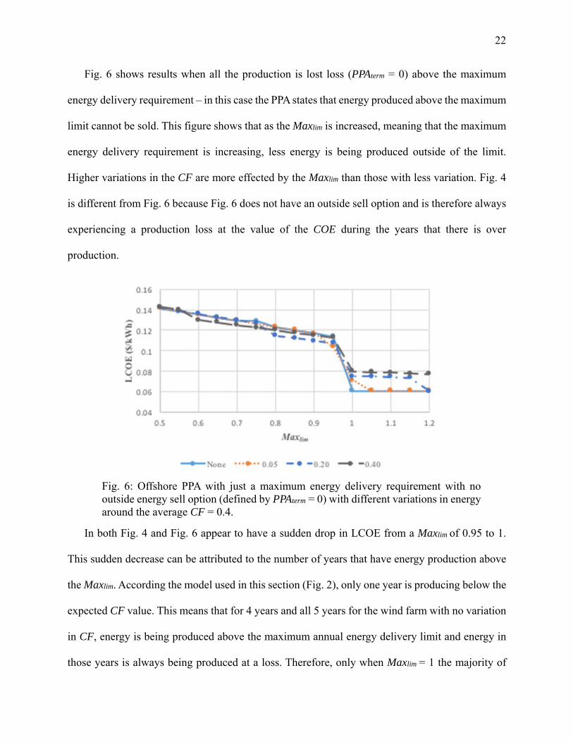
Fig. 6 shows results when all the production is lost loss (PPAterm = 0) above the maximum

energy delivery requirement – in this case the PPA states that energy produced above the maximum

limit cannot be sold. This figure shows that as the Maxlim is increased, meaning that the maximum

energy delivery requirement is increasing, less energy is being produced outside of the limit.

Higher variations in the CF are more effected by the Maxlim than those with less variation. Fig. 4

is different from Fig. 6 because Fig. 6 does not have an outside sell option and is therefore always

experiencing a production loss at the value of the COE during the years that there is over

production.

In both Fig. 4 and Fig. 6 appear to have a sudden drop in LCOE from a Maxlim of 0.95 to 1.

This sudden decrease can be attributed to the number of years that have energy production above

the Maxlim. According the model used in this section (Fig. 2), only one year is producing below the

expected CF value. This means that for 4 years and all 5 years for the wind farm with no variation

in CF, energy is being produced above the maximum annual energy delivery limit and energy in

those years is always being produced at a loss. Therefore, only when Maxlim = 1 the majority of

Fig. 6: Offshore PPA with just a maximum energy delivery requirement with no outside energy sell option (defined by PPAterm = 0) with different variations in energy around the average CF = 0.4.

23

years are not producing above the limit. Even at Maxlim = 1, one year for every wind farm, except

the wind farm without variation, there is a higher than the expected CF. Due to this one year, the

LCOE for the wind farm without variation is lower than the LCOEs for the wind farms with

variation at Maxlim = 1.

There is another type of PPA that was not presented in this section, which is a PPA that contains

both a Maxlim and a Minlim. This PPA follows almost the same conditions and requirements for both

limits. The only difference is that the Maxlim can never be lower than the Minlim. Generally, in a

PPA containing both limits, there is enough of a gap between the limits for energy to fall between

them, but Minlim can never be larger than Maxlim or all energy produced will always be penalized.

The case of a PPA with both limits is considered in the wind farm cast study in the next section.

WIND FARM CASE STUDY

This section explores the actual LCOEs produced for a set of real wind farms (real CF

histories). All the cases in this section use identical contract variables, requirements on energy

delivery, and COE. The purpose of this wind farm case study is to evaluate the effects of using the

same PPA on farms that vary in location and energy production. Four PPA options are considered.

First a PPA with no energy delivery limits, where the energy is bought and sold as it is produced.

The first type of PPA reflects a conventional LCOE where the PPA energy delivery limits are not

applied. The second PPA has only a minimum delivery limit where energy is not allowed to be

purchased or sold in the spot market after that limit has been reached. The third PPA has just a

maximum delivery limit, and the fourth PPA has both delivery limits. Real data was collected

from 7 different wind farms (Table 1[31]) that have different numbers of turbines, manufacturers,

years built, rated power and country (Germany or Denmark). The data from Germany and

24

Denmark was readily available from established wind farms with long enough history of data

collection to be viable for consideration in the study. All the costs used in the model

Wind Farm Dataset/Manufacturer/Rated Power

Year Built Location (Number of Turbines)

1 - Vestas (2 MW) 2002 Germany (17)

2 - Enercon (2 MW) 2005 Germany (24)

3 - Siemens (2.3 MW) 2010 Denmark (11)

4 - Enercon (2 MW) 2010 Germany (10)

5 - Vestas (3 MW) 2010 Denmark (18)

6 - Vestas (3 MW) 2007 Germany (5)

7 - Siemens (3.6 MW) 2006 Germany (7)

Table 1 - Wind farm dataset details[31].

25

verification tests were used in this case study except a fixed COE for each farm of $0.25 per kWh,

based on NREL’s highest expected COE in wind farms from 2025-2050[32] is used in this case

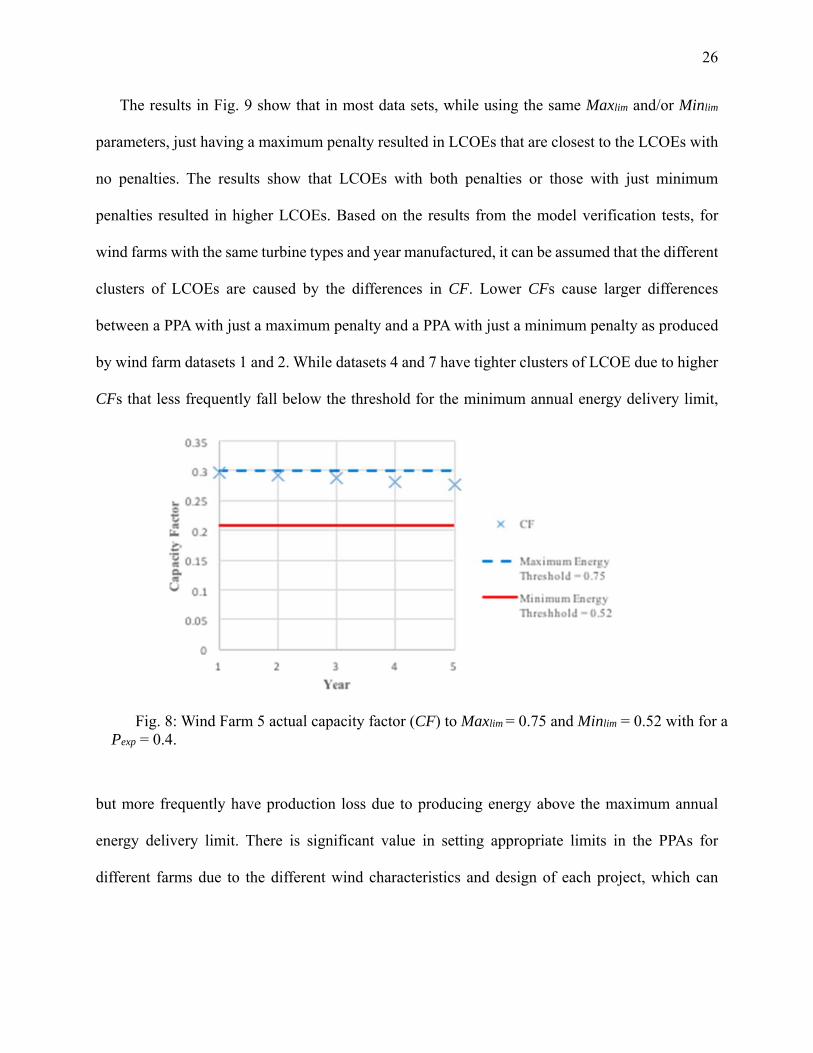
study. The four different PPA types assume Maxlim = 0.75 and a Minlim = 0.52.8 Figs. 7 and 8 portray

two different wind farms actual CF compared to the Maxlim and Minlim used in the PPAs. The

figures show that using the same annual energy delivery quantities on two different farms

potentially produce different results due to the different actual annual CF variation. The farm in

Fig. 7 has more variation in CF than the farm in Fig. 8, where the CF of the wind farm is nearly

constant from year to year. The LCOE of each turbine was calculated from the sum of LCOE costs

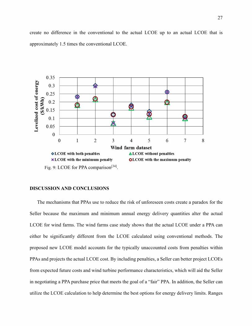
at the end of 5 years. Fig. 9 shows the LCOEs based on the different annual energy delivery

requirements and the selection of penalties that were applied.

8 The values of Maxlim = 0.75 and Minlim = 0.52 are based on limits previously used in Zhu[33] and Delmarva Power

and Light Company and Bluewater Wind Delaware LLC Power Purchase Agreement[20].

Fig. 7: Wind Farm 3 actual CF to Maxlim = 0.75 and Minlim = 0.52 with for a Pexp =

0.4.

26

The results in Fig. 9 show that in most data sets, while using the same Maxlim and/or Minlim

parameters, just having a maximum penalty resulted in LCOEs that are closest to the LCOEs with

no penalties. The results show that LCOEs with both penalties or those with just minimum

penalties resulted in higher LCOEs. Based on the results from the model verification tests, for

wind farms with the same turbine types and year manufactured, it can be assumed that the different

clusters of LCOEs are caused by the differences in CF. Lower CFs cause larger differences

between a PPA with just a maximum penalty and a PPA with just a minimum penalty as produced

by wind farm datasets 1 and 2. While datasets 4 and 7 have tighter clusters of LCOE due to higher

CFs that less frequently fall below the threshold for the minimum annual energy delivery limit,

but more frequently have production loss due to producing energy above the maximum annual

energy delivery limit. There is significant value in setting appropriate limits in the PPAs for

different farms due to the different wind characteristics and design of each project, which can

Fig. 8: Wind Farm 5 actual capacity factor (CF) to Maxlim = 0.75 and Minlim = 0.52 with for a

Pexp = 0.4.

27

create no difference in the conventional to the actual LCOE up to an actual LCOE that is

approximately 1.5 times the conventional LCOE.

DISCUSSION AND CONCLUSIONS

The mechanisms that PPAs use to reduce the risk of unforeseen costs create a paradox for the

Seller because the maximum and minimum annual energy delivery quantities alter the actual

LCOE for wind farms. The wind farms case study shows that the actual LCOE under a PPA can

either be significantly different from the LCOE calculated using conventional methods. The

proposed new LCOE model accounts for the typically unaccounted costs from penalties within

PPAs and projects the actual LCOE cost. By including penalties, a Seller can better project LCOEs

from expected future costs and wind turbine performance characteristics, which will aid the Seller

in negotiating a PPA purchase price that meets the goal of a “fair” PPA. In addition, the Seller can

utilize the LCOE calculation to help determine the best options for energy delivery limits. Ranges

Fig. 9: LCOE for PPA comparison[34].

28

in penalties will be determined by the Buyer’s need to reduce risk of over-paying for energy

production or under-delivering to the market. The Seller can utilize the new model to determine

the most appropriate PPA type and penalties given the limitations set by the Buyer and the desired

LCOE. Without a correctly calculated LCOE, the project could fail, negatively affecting both the

Seller and the Buyer as the Buyer is expecting to meet consumer needs using the Seller’s generated

energy. The model has been developed for any combination of penalties imposed by a PPA. By

changing the data inputs, users can apply the model to anywhere in the world.

This model makes several simplifying assumptions and changes to the assumed variables can

have significant effects to the LCOE. Typically, the model is used to project the LCOE of an energy

project. This requires estimating energy production, which is difficult to predict for renewable

energy sources. We assume a constant WACC, which is a dynamic and difficult to predict variable,

the use of a constant PPA price schedule and no escalating price schedule, and simplified O&M

costs that do not account for a required O&M schedule in a PPA or O&M costs for wind turbine

failure. Decommissioning costs were not included in the model in this paper because we assumed

that there could be additional PPAs following the ones analyzed that would encompass

decommissioning if relevant. Fundamentally, this paper still considers the LCOE to be a constant

although it can change based on the length of the PPA versus the actual lifetime of a

project[16][17][18]. In some cases, the LCOE might not be used to determine COE in a PPA. While

LCOE is the most commonly known and used, some projects may use other methods to calculate

the break-even cost of the project, such as the Levelized Avoided Cost of Energy (LACE)[35].

A new concept called a “synthetic PPA” has recently appeared. Synthetic PPAs use hedges to

ensure a preferred financing method around spot-market prices without the actual purchase of

energy from the hedge. There are structures common to synthetic PPAs such as: Contracts-for-

29

Differences (CfDs), Call options, Put options, Collars, and Commodity hedges[4]. CfDs are

contracts that guarantee each unit of energy will be sold at a single strike price. The project will

sell the power into the direct and open market and the offtaker will purchase the power from the

open market. If the price falls above the strike price, then the hedge compensates the difference to

the offtaker. On the other hand, if the spot-market price falls below the open-market price than the

offtaker will compensate the hedge. Call options, Put options, and Collars are all examples of

synthetic PPAs known as Options. Options provide the project with the option to be to purchase

the energy at the strike price if the market price falls below the strike price. Hedges can also

mitigate electricity price fluctuations by hedging the price of commodities. Given these differing

types of synthetic PPA structures, it is obvious that more complex models for evaluating LCOE

than the model presented in this paper could be developed.

Renewable energy credits can function similarly to PPAs. For example, in the Maryland

Offshore Renewable Energy Credits (ORECs), allow offshore wind to contribute a maximum of

2.5% of the total residential energy used in Maryland each year into the regional energy

market[6][36]. In the Maryland model, a wind farm must submit an application for the value and

quantity of ORECs required to meet this restriction. The ORECs have a maximum limit, but

Equation (11) would have to be altered to reflect annual residential energy consumption instead of

the expected energy generation. Currently, two planned wind farms (Skipjack and US Wind) have

been awarded Maryland ORECs that together, produce under the 2.5% residential energy

consumption limit. However, the awarded OREC quantity to each farm, reflecting the average

energy production and the OREC price as determined by the LCOE, was calculated assuming

constant energy generation. Wind energy production is not constant and as seen in the study, there

can be significant difference between the conventionally calculated LCOE and the actual LCOE.

30

Policies such as the Maryland ORECs, where renewable energy is limited to be sold at a specific

quantity, should consider the variation in energy production and its effect on the actual LCOE so

a fair price for energy can be awarded.

ACKNOWLEDGEMENTS

Funding for this work was provided by Exelon for the advancement of Maryland's offshore

wind energy and jointly administered by MEA and MHEC, as part of “Maryland Offshore Wind

Farm Integrated Research (MOWFIR): Wind Resources, Turbine Aeromechanics, Prognostics and

Sustainability”.

REFERENCES

[1] Short, W., Packey, D., & Holt, T. (1995). “A Manual for the Economic Evaluation of

Energy Efficiency and Renewable Energy Technologies,” NREL/TP-462-5173, March 1995

[2] European Wind Energy Association (2013). “Where’s the money coming from? Financing offshore wind farms,” Last Accessed: January 27, 2017. Available at: http://www.ewea.org/fileadmin/files/library/publications/reports/Financing_Offshore_Wind_Farms.pdf

[3] U.S. Department of Energy, Energy Efficiency and Renewable Energy (2015). 2015 Wind

Technologies Market Report.

[4] Baker & McKenzie (n.d.). “The rise of corporate PPAs: A new driver for renewables,” Clean Energy Pipeline. Available at: http://www.cleanenergypipeline.com/Resources/CE/ResearchReports/the-rise-of-corporate-ppas.pdf

[5] Norton Rose Fulbright (2016). “Renewable energy in Latin America,” Last Accessed:

January 27, 2017. Available at: http://www.nortonrosefulbright.com/files/renewable-energy-in-latin-america-134675.pdf

[6] Wiser, R., Namovicz, C., Gielecki, M., & Smith, R. (2007). “The Experience with

Renewable Portfolio Standards in the United States,” The Electricity Journal, Vol. 20, No. 4, pp. 8-20.

31

[7] Adarmola, M., Paul, S., & Oyedepo, S. (2011). “Assessment of Electricity Generation and Energy Cost of Wind Energy Conversion Systems in North-Central Nigeria,” Energy Conversion and Management, Vol. 52, No. 12, pp. 3363-3368.

[8] SAM Help. (n.d.). Last Accessed: December 22, 2015. Available at:

https://www.nrel.gov/analysis/sam/help/html-php/index.html?mtf_lcoe.htm

[9] Ragheb, M. (2015). “Economics of Wind Energy,” Last Accessed: December 21, 2015. Available at: http://mragheb.com/NPRE%20475%20Wind%20Power%20Systems/Economics%20of%20Wind%20Energy.pdf

[10] Filipa, F., Pina, L., Wemans, J., Sorasio, G., & Brito, M. (2014). “LCOE Analysis as a

Decision Tool for Design of Concentrated Photovoltaics Systems,” Proceedings, 26th European Photovoltaic Solar Energy Conference and Exhibition, Session 6CV.1.28, pp. 4581-4583.

[11] Fotster, J., Wagner, L., & Baratanova, A. (2014). “LCOE models: A comparison of the

theoretical frameworks and key assumptions,” Energy Economics and Management Group Working Papers from School of Economics, University of Queensland Australia, No. 4

[12] Myhr, A., Bjerkseter, C., Agotnes, A., Nygaard, T. (2014).”Levelised cost of energy for

offshore floating wind turbines in a life cycle perspective.” Renewable Energy. Vol. 66, pp. 714-728

[13] Cory, K., Canavan, B., & Koenig, R. (2009). “Power Purchase Agreement Checklist for

State and Local Governments,” National Renewable energy Laboratory Fact Sheet Series. Last Accessed: December 20, 2015/ Available at: http://www.nrel.gov/docs/fy10osti/46668.pdf

[14] Hernandez, K., Richard, & C., Nathwani, J. (2016). “Estimating Project LCOE – an

Analysis of Geothermal PPA Data,” Proceedings 41st Workshop on Geothermal Reservoir Engineering, Stanford University, Stanford, California, February 22-24, 2016 SGP-TR-209.

[15] Islamic Republican of Pakistan Standardized Energy Purchase Agreement Draft (2006).

[16] Aswathanarayana, U., Harikrishnan, T., & Kadher-Mohein, T. (2010). Green Energy:

Technology, Economics and Policy, CRC Press, Taylor and Francis Group, Boca Raton, FL, pp. 241.

[17] Bacon, R., & Besant-Jones, J. (2001). “Global Electrical power Reform Privatization, and

Liberalization of the Electrical Power Industry in Developing Countries,” Annual Review of Energy and the Environment, Vol. 26, No. 1, pp. 331-359.

32

[18] Ryor, J., & Tawney, L. (n.d.). “Understanding Renewable Energy Cost Parity,” World Resources Institute Fact Sheet. Last Accessed: December 23, 2015. Available at: http://www.wri.org/publication/understanding-renewable-energy-cost-parity

[19] State of Maryland Office of People’s Counsel (2017). “Case No. 9431: Direct Testimony

of Maximilian Chang

[20] Delmarva Power and Light Company and Bluewater Wind Delaware LLC Power Purchase Agreement (June 23, 2008).

[21] Regional Center for Renewable Energy and Energy Efficiency (2012). “User’s Guide for The Power Purchase Agreement (PPA) Model for Electricity from Renewable Energy Facilities,” Last Accessed: December 20, 2015. Available at: http://www.rcreee.org/sites/default/files/users_guide_ppa_reegf.pdf

[22] PacifiCorp Power Purchase Agreement Draft

[23] U.S. Department of energy (2015). “Wind Vision: A New Era for Wind Power in the

United States.”

[24] Fraunhofer Institute for Solar Energy Systems ISE (2013). “Levelized Cost of Electricity Renewable Energy Technologies.”

[25] IFC International Administration (2010). The Cost and Performance of Distributed Wind

Turbines 2010-35 Final Report.

[26] Fulton, M. (2012) . “The German Feed-In Tariff: Recent Policy Changes,” Deutsche Bank Group. Last Accessed December 20, 2015. Available at: https://www.dbresearch.com/PROD/DBR_INTERNET_EN-PROD/PROD0000000000294376/The+German+Feed-in+Tariff%3A+Recent+Policy+Changes.PDF

[27] National Renewable Energy Laboratory (2015). “Annual Technology Baseline Presentation,” Last Accessed: December 22, 2015. Available at: http://www.nrel.gov/docs/fy15osti/64077.pdf

[28] James-Smith, E. (2011b). Development in LCOE for Wind Turbines in Denmark.

Presentation to IEA Wind Task 26

[29] Lantz, E., Wiser, R., & Hand, M. (2012). “The Past and Future Cost Of Wind Energy,” IEA Wind Task 26.

[30] U.S. Energy Information Administration (2014). “Historical wholesale market data,”

Electricity, Wholesale Electricity and Natural Gas Market Data. Last Accessed: February 20, 2017. Available at: https://www.eia.gov/electricity/wholesale/

33

[31] Windstats, Quarterly Report (2011-2014) ISSN 0903-5648 Vol. 24 – 28

[32] Blair, N., Cory. K., Hand, M., Parkhill, L., Speer, B., Stehly, T., Feldman, D., Lantz, E., Augustine, C., Turchi, C., & O’Connor, P. (2015). “Annual Technology Baseline,” Presentation and Supporting Data Set, National Renewable Energy Laboratory. Available at: http://www.nrel.gov/analysis/pdfs/ATB_Summary_V13.pdf

[33] Zhu, X. (2014). “Offtake Strategy on Design for Wind Energy Projects Under Certainty,”

Ph.D. Dissertation, Department of Civil and Environmental Engineering, University of Maryland, College Park.

[34] Bruck, M., Goudarzi, N., & Sandborn, P. (2016). “A Levelized Cost of Energy (LCOE)

Model for Wind Farms That Includes Power Purchase Agreement (PPA) Energy Delivery Limits,” ASME 2016 Power Conference Paper Proceedings, June 26-30, 2016.

[35] U.S. Energy Information Administration (2014). “Levelized Cost and Levelized Avoided

Cost of New Generation Resources in the Annual Energy Outlook (2014).”

[36] Public Service Commission of Maryland (2104). “Ten-Year Plan (2014-2023) of Electric Companies in Maryland,” Available at: http://webapp.psc.state.md.us/intranet/Reports/2014%20-%202023%20TYP%20Final.pdf