Embed Size (px)
Citation preview
A high-order discontinuous-Galerkin octree-based AMR solver for
overset simulations
Michael J. Brazella, Andrew C. Kirbyb, and Dimitri J. Mavriplisc
Department of Mechanical Engineering
University of Wyoming
The goal of this work is to develop a highly efficient off-body solver for use in oversetsimulations. Overset meshes have been gaining traction in recent years and are beingused increasingly to simulate very complex large-scale problems. In particular we focuson a dual-mesh, dual-solver overset approach that combines specialized flow solvers indifferent regions of the flow domain: near-body and off-body. The near-body flow solver isdesigned to handle complicated geometry, anisotropic elements, and unstructured meshes.In contrast, the off-body solver is designed to be high-order, Cartesian, and use adaptivemesh refinement (AMR). The high-order discretization used for the off-body solver isbased on the discontinuous Galerkin (DG) method. To get the most efficiency out of themethod, a Cartesian grid is employed and tensor product basis functions are used in the DGformulation. The dense computational kernels allow this solver to obtain a near-constantcost per degree of freedom for a wide range of p-orders of accuracy. To further enhancethe capabilities of the off-body solver, the DG solver in linked to an octree-based AMRlibrary called p4est; this gives the ability for h-adaptation via non-conforming elements.p-adaption is also implemented in which each cell can be assigned a different polynomialdegree basis. Combined h and p refinement is necessary for overlapping mesh problemswhere the off-body solver mesh must connect to the low-order near-body solver, sinceboth mesh resolution and order of accuracy must be matched in the overlapping regions.To demonstrate the efficiency, accuracy, and capabilities of the DG AMR flow solver wesimulate Ringleb flow and the Taylor-Green vortex problem. Finally, to demonstrate theoverset capabilities a NACA 0015 wing case and a NREL PhaseVI wind turbine case aresimulated.
I. Introduction
Overset mesh approaches have been used for many years in computational fluid dynamics due to theflexibility they afford for handling complex geometries and simulations involving bodies with relative motionsuch as store separation, rotorcraft, and wind turbine configurations.1–4 Most overset mesh applicationsinvolve the use of similar mesh components, i.e. either structured meshes overlapped with structured meshes5
or collections of overlapping unstructured meshes.6 More recently, frameworks that support combinations ofdifferent types of overlapping meshes have been developed. One example is the HELIOS rotorcraft software,4
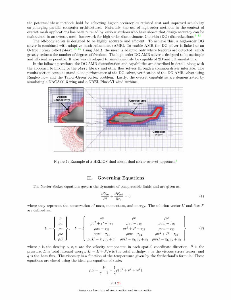
which supports arbitrary combinations of unstructured, structured, and Cartesian meshes, along with thedifferent discretizations used on these meshes. Figure 1 shows a dual-mesh dual-solver overset frameworkused by HELIOS where there is an unstructured near-body mesh and a Cartesian AMR off-body mesh.HELIOS applications have shown how the use of adaptively refined Cartesian meshes in off-body regionscan be enabling for capturing wakes and vortices with high levels of accuracy.4,7, 8 High-order accuratediscretizations have generated much interest over the last decade for computational aerodynamics due to
aAIAA member, Research Scientist, [email protected] member, Ph.D. Candidate, [email protected] Associate Fellow, Professor, [email protected]
1
the potential these methods hold for achieving higher accuracy at reduced cost and improved scalabilityon emerging parallel computer architectures. Naturally, the use of high-order methods in the context ofoverset mesh applications has been pursued by various authors who have shown that design accuracy can bemaintained in an overset mesh framework for high-order discontinuous Galerkin (DG) discretizations.9–12
The off-body solver is designed to be highly accurate and efficient. To achieve this, a high-order DGsolver is combined with adaptive mesh refinement (AMR). To enable AMR the DG solver is linked to anOctree library called p4est.13–15 Using AMR, the mesh is adapted only where features are detected, whichgreatly reduces the number of degrees of freedom. The high-order DG AMR solver is designed to be as simpleand efficient as possible. It also was developed to simultaneously be capable of 2D and 3D simulations.
In the following sections, the DG AMR discretization and capabilities are described in detail, along withthe approach to linking to the p4est library and other flow solvers through a common driver interface. Theresults section contains stand-alone performance of the DG solver, verification of the DG AMR solver usingRingleb flow and the Taylor-Green vortex problem. Lastly, the overset capabilities are demonstrated bysimulating a NACA 0015 wing and a NREL PhaseVI wind turbine.
Figure 1: Example of a HELIOS dual-mesh, dual-solver overset approach.4
II. Governing Equations
The Navier-Stokes equations govern the dynamics of compressible fluids and are given as:
∂Um
∂t+∂Fmi
∂xi= 0 (1)
where they represent the conservation of mass, momentum, and energy. The solution vector U and flux Fare defined as:
U =
ρ
ρu
ρv
ρw
ρE
, F =
ρu ρv ρw
ρu2 + P − τ11 ρuv − τ12 ρuw − τ13
ρuv − τ21 ρv2 + P − τ22 ρvw − τ23
ρuw − τ31 ρvw − τ32 ρw2 + P − τ33
ρuH − τ1juj + q1 ρvH − τ2juj + q2 ρwH − τ3juj + q3
(2)
where ρ is the density, u, v, w are the velocity components in each spatial coordinate direction, P is thepressure, E is total internal energy, H = E + P/ρ is the total enthalpy, τ is the viscous stress tensor, andq is the heat flux. The viscosity is a function of the temperature given by the Sutherland’s formula. Theseequations are closed using the ideal gas equation of state:
ρE =P
γ − 1+
1
2ρ(u2 + v2 + w2)
2 of 28
American Institute of Aeronautics and Astronautics
where γ = 1.4 is the ratio of specific heats. Einstein notation is used where the subscripts of i and j representspatial dimensions and have a range of 1 to 3 and the indices of m and n vary over the number of variables.
III. Off-body DG AMR solver formulation
In this section the DG finite element formulation used to solve the Navier-Stokes equations is described.The DG kernel that is responsible for the physics and discretization is referred to as CartDG.16 To derivethe weak form, equation (1) is first multiplied by a test function φr and integrated over the domain Ω toobtain the weak form: ∫
Ω
φr
(∂Um
∂t+∂Fmi
∂xi
)dΩ = 0.
Integration by parts is performed and the residual Rmr is defined as:
Rmr =
∫Ω
(φr∂Um
∂t− ∂φr∂xi
Fmi
)dΩ +
∫Γ
φrFminidΓ = 0
where φr are the basis functions and the solution is approximated using Um = φsams. The indices r and srun over the number of basis functions. The basis functions used in this formulation are tensor products of1D Lagrange polynomials. To construct these Lagrange polynomials a nodal basis is formed on the Gauss-Legendre quadrature points. This creates a highly efficient nodal collocated basis function where each basisfunction equals one at a quadrature point and zero on the remaining quadrature points.
The residual now contains integrals over faces Γ and special treatment is needed for the fluxes in theseterms. The advective fluxes are calculated using a Lax-Friedrichs flux.17 The diffusive fluxes are handledusing a symmetric interior penalty (SIP) method.18,19 For the temporal discretization high-order explicitRunge-Kutta schemes are used including the standard RK420 and SSP RK2.21 These schemes are used onsystems of ODE’s so the residual formulation is rearranged to be:
Mmrns∂ans∂t
=
∫Ω
∂φr∂xi
FmidΩ−∫
Γ
φrFminidΓ
where Mmrns is a mass matrix and the right hand side now contains only spatial residual terms. The massmatrix is inverted to create a system of ODE’s. The Lagrange basis functions used in this formulation forma diagonal mass matrix is which makes inversion trivial.
A. Tensor formulation
The main goal of this work is to develop a highly efficient high-order accurate off-body solver. To do thiswe have made the simplification that the domain is comprised of purely Cartesian hexahedral elements. Anefficient set of basis functions for hexahedral elements are tensor product Lagrange polynomials collocatedon Gauss-Legendre quadrature points. This formulation is commonly called DGSEM and comes from thecombination of the DG discretization and the spectral element method (SEM).22–25 This allows for manysimplifications in both the projection and integration routines. For a standard finite element method withno simplifications an integration and projection routine takes O((p+ 1)6) operations. A solution projectionis defined as:
U(ξ, η, ζ) =
p+1∑r,s,t=0
ψrst (ξ, η, ζ) arst
where an inner product of the basis functions with the solution coefficients requires O((p + 1)3) work foreach quadrature point. In the case that the number of quadrature points is equal to the number of basisfunctions this equates to O((p + 1)6) work per cell. Since ψ is a tensor product of one-dimensional basisfunctions we can expand it to be:
ψrst(ξ, η, ζ) = `r(ξ)`s(η)`t(ζ)
where `(ξ) is a one-dimensional Lagrange polynomial:
`j(ξ) =
p+1∏i=0,i6=j
(ξ − ξi)(ξj − ξi)
3 of 28
American Institute of Aeronautics and Astronautics
where ξi are the Gauss-Legendre quadrature points and has the property:
`j(ξi) = δij
at the quadrature points. Therefore, the projection becomes:
U(ξi, ηj , ζk) =
p+1∑r,s,t=0
`r(ξi)`s(ηj)`t(ζk) arst
and simplifies to:
U(ξi, ηj , ζk) =
p+1∑r,s,t=0
δriδsjδtk arst = aijk.
The projection work reduces to O((p+ 1)3) operations.A volume integral has a similar simplification, we begin by looking at one term in the weighted integral
form:
Rv1mrst =
∫ 1
−1
∫ 1
−1
∫ 1
−1
∂ψrst
∂ξFm1dξdηdζ
where Rv1mrst is a single volume residual for a particular element in the ξ-direction. The tensor basis is
introduced to give:
=
∫ 1
−1
∫ 1
−1
∫ 1
−1
∂`r(ξ)
∂ξ`s(η)`t(ζ)Fm1dξdηdζ.
The integrals are approximated using Gauss-Legendre quadrature rules:
'p+1∑
i,j,k=0
∂`r(ξi)
∂ξ`s(ηj)`t(ζk)Fm1(ξi, ηj , ζk)wiwjwk
where w are the quadrature weights. Simplifying further we arrive at:
=
p+1∑i,j,k=0
∂`r(ξi)
∂ξδjsδktFm1(ξi, ηj , ζk)wiwjwk
and finally due to collocation:
=
p+1∑i=0
∂`r(ξi)
∂ξFm1(ξi, ηs, ζt)wiwswt
where only a one-dimensional summation remains. The integral is performed for (p+1)3 basis functions andso the work for this particular integral reduces from O((p+ 1)6) to O((p+ 1)4) operations.
A detailed summary of the total work and memory for each operation in the DGSEM method is shown inRef.25 The combination of tensor products and collocation creates a large reduction in the total number offloating point operations. However, at lower polynomial degrees the flop rate is higher for the naive approachsince the operations can be converted into matrix-matrix products. Therefore, at lower polynomial degreesthe naive approach can be faster overall, especially when using linear-algebra libraries such as BLAS. Thispolynomial degree crossover point will depend on the hardware and the implementation and is thoroughlystudied in Ref.26 A demonstration of this will be shown in the next section in a discussion of the performanceof CartDG.
B. CartDG stand-alone performance
CartDG is designed for high computational efficiency. To achieve this, high-order finite-element discretiza-tions are preferred in order capitalize on the dense computational kernels associated with these discretizations,while taking advantage of matrix-matrix multiplication implementations when possible. The discretizationis based on a nodal, collocated tensor basis embedded in a Cartesian coordinate system.
The mass matrix of a nodal, collocated basis forms a diagonal, static matrix meaning that the massmatrix does not change over the duration of the simulation. Many implementations of the DG method
4 of 28
American Institute of Aeronautics and Astronautics
involve a matrix multiplication of the inverted mass matrix and the spatial residual vector. Since the inversemass matrix is static over the duration of the simulation, it can be pre-multiplied into the basis functionsthat are used to construct the spatial residual vector therefore saving a matrix-vector multiplication at everyresidual evaluation.
By restricting the discretization to a Cartesian coordinate system, further simplifications can be intro-duced. The element Jacobian which is used to transform the solution in physical space to reference spaceis constant for every cell with cell width δx. Therefore, the element Jacobian is constant and can alsobe pre-multiplied into the basis functions used to construct the spatial residual vector. Additionally, sincethe normal vectors in a Cartesian coordinate system only contain one component, e.g. n=(1,0,0), special-ized routines for flux calculations are constructed for each coordinate direction that eliminate floating pointoperations related to the orthogonal coordinates.
Advanced vectorization and data alignment techniques are employed throughout the implementation.At higher polynomial degrees it is advantageous to rearrange the solution order in memory. Traditionally,for column-major memory storage, the solution vector is stored by ordering fields first, followed by modesand elements, where the fields are the conservative flow variables and the modes are the polynomial modes.However, in order to perform single-instruction-multiplie-data (SIMD) vectorization of flux calculations,reordering the storage to modes, fields and elements is needed. When this action is performed, vectorizationallows for either two, four, or eight flux evaluations to be performed in parallel with the Intel AVX, AVX-2,or AVX-512 vector instructions, respectively.
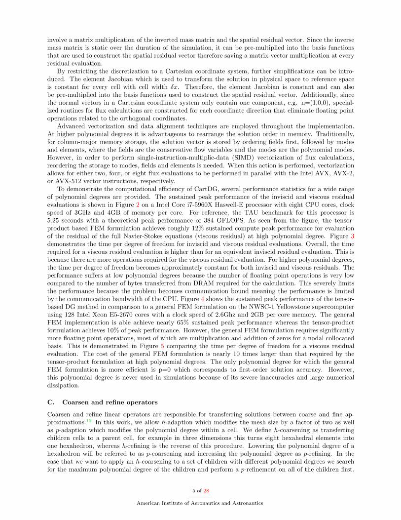
To demonstrate the computational efficiency of CartDG, several performance statistics for a wide rangeof polynomial degrees are provided. The sustained peak performance of the inviscid and viscous residualevaluations is shown in Figure 2 on a Intel Core i7-5960X Haswell-E processor with eight CPU cores, clockspeed of 3GHz and 4GB of memory per core. For reference, the TAU benchmark for this processor is5.25 seconds with a theoretical peak performance of 384 GFLOPS. As seen from the figure, the tensor-product based FEM formulation achieves roughly 12% sustained compute peak performance for evaluationof the residual of the full Navier-Stokes equations (viscous residual) at high polynomial degree. Figure 3demonstrates the time per degree of freedom for inviscid and viscous residual evaluations. Overall, the timerequired for a viscous residual evaluation is higher than for an equivalent inviscid residual evaluation. This isbecause there are more operations required for the viscous residual evaluation. For higher polynomial degrees,the time per degree of freedom becomes approximately constant for both inviscid and viscous residuals. Theperformance suffers at low polynomial degrees because the number of floating point operations is very lowcompared to the number of bytes transferred from DRAM required for the calculation. This severely limitsthe performance because the problem becomes communication bound meaning the performance is limitedby the communication bandwidth of the CPU. Figure 4 shows the sustained peak performance of the tensor-based DG method in comparison to a general FEM formulation on the NWSC-1 Yellowstone supercomputerusing 128 Intel Xeon E5-2670 cores with a clock speed of 2.6Ghz and 2GB per core memory. The generalFEM implementation is able achieve nearly 65% sustained peak performance whereas the tensor-productformulation achieves 10% of peak performance. However, the general FEM formulation requires significantlymore floating point operations, most of which are multiplication and addition of zeros for a nodal collocatedbasis. This is demonstrated in Figure 5 comparing the time per degree of freedom for a viscous residualevaluation. The cost of the general FEM formulation is nearly 10 times larger than that required by thetensor-product formulation at high polynomial degrees. The only polynomial degree for which the generalFEM formulation is more efficient is p=0 which corresponds to first-order solution accuracy. However,this polynomial degree is never used in simulations because of its severe inaccuracies and large numericaldissipation.
C. Coarsen and refine operators
Coarsen and refine linear operators are responsible for transferring solutions between coarse and fine ap-proximations.15 In this work, we allow h-adaption which modifies the mesh size by a factor of two as wellas p-adaption which modifies the polynomial degree within a cell. We define h-coarsening as transferringchildren cells to a parent cell, for example in three dimensions this turns eight hexahedral elements intoone hexahedron, whereas h-refining is the reverse of this procedure. Lowering the polynomial degree of ahexahedron will be referred to as p-coarsening and increasing the polynomial degree as p-refining. In thecase that we want to apply an h-coarsening to a set of children with different polynomial degrees we searchfor the maximum polynomial degree of the children and perform a p-refinement on all of the children first.
5 of 28
American Institute of Aeronautics and Astronautics
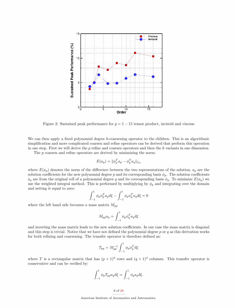
Figure 2: Sustained peak performance for p = 1− 15 tensor product, inviscid and viscous
We can then apply a fixed polynomial degree h-coarsening operator to the children. This is an algorithmicsimplification and more complicated coarsen and refine operators can be derived that perform this operationin one step. First we will derive the p refine and coarsen operators and then the h variants in one dimension.
The p coarsen and refine operators are derived by minimizing the norm:
E(ap) = ‖φTp ap − φTq aq‖L2
where E(ap) denotes the norm of the difference between the two representations of the solution, ap are thesolution coefficients for the new polynomial degree p and its corresponding basis φp. The solution coefficientsaq are from the original cell of a polynomial degree q and its corresponding basis φq. To minimize E(ap) weuse the weighted integral method. This is performed by multiplying by φp and integrating over the domainand setting it equal to zero: ∫ 1
−1
φpφTp apdξ −
∫ 1
−1
φpφTq aqdξ = 0
where the left hand side becomes a mass matrix Mpp
Mppap =
∫ 1
−1
φpφTq aqdξ
and inverting the mass matrix leads to the new solution coefficients. In our case the mass matrix is diagonaland this step is trivial. Notice that we have not defined the polynomial degree p or q as this derivation worksfor both refining and coarsening. The transfer operator is therefore defined as:
Tpq = M−1pp
∫ 1
−1
φpφTq dξ
where T is a rectangular matrix that has (p + 1)d rows and (q + 1)d columns. This transfer operator isconservative and can be verified by: ∫ 1
−1
φpTpqaqdξ =
∫ 1
−1
φqaqdξ.
6 of 28
American Institute of Aeronautics and Astronautics
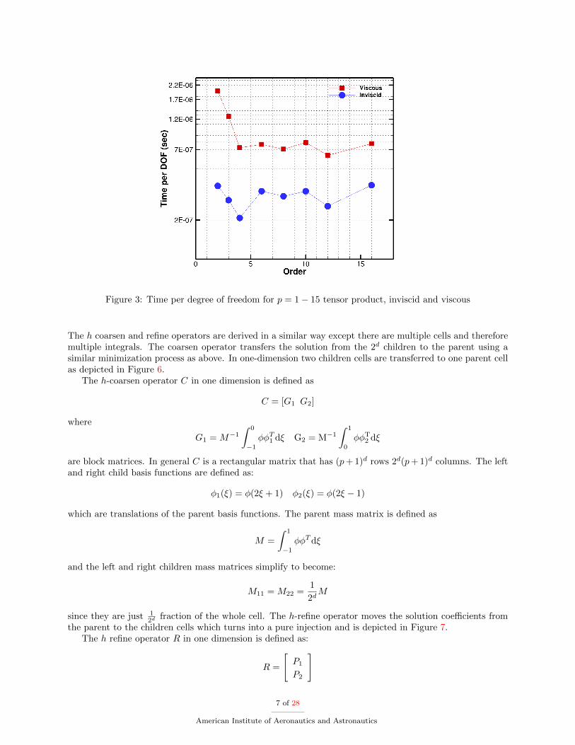
Figure 3: Time per degree of freedom for p = 1− 15 tensor product, inviscid and viscous
The h coarsen and refine operators are derived in a similar way except there are multiple cells and thereforemultiple integrals. The coarsen operator transfers the solution from the 2d children to the parent using asimilar minimization process as above. In one-dimension two children cells are transferred to one parent cellas depicted in Figure 6.
The h-coarsen operator C in one dimension is defined as
C = [G1 G2]
where
G1 = M−1
∫ 0
−1
φφT1 dξ G2 = M−1
∫ 1
0
φφT2 dξ
are block matrices. In general C is a rectangular matrix that has (p+ 1)d rows 2d(p+ 1)d columns. The leftand right child basis functions are defined as:
φ1(ξ) = φ(2ξ + 1) φ2(ξ) = φ(2ξ − 1)
which are translations of the parent basis functions. The parent mass matrix is defined as
M =
∫ 1
−1
φφT dξ
and the left and right children mass matrices simplify to become:
M11 = M22 =1
2dM
since they are just 12d fraction of the whole cell. The h-refine operator moves the solution coefficients from
the parent to the children cells which turns into a pure injection and is depicted in Figure 7.The h refine operator R in one dimension is defined as:
R =
[P1
P2
]
7 of 28
American Institute of Aeronautics and Astronautics

Figure 4: Tensor basis and general FEM performance peak for p = 1− 15
where
P1 = M−111
∫ 0
−1
φ1φT dξ, P2 = M−1
22
∫ 1
0
φ2φTdξ.
In general R is a rectangular matrix that has 2d(p+ 1)d rows and (p+ 1)d columns. It follows that applyinga refine and then a coarsen operator should return the original coefficients:
a = CRa
which is equivalent to the property that:CR = I.
It is also important to maintain conservation with these operations. The h-coarsen operator holds thisconservation property that the sum of the average cell quantity of the children cells equals the average cellquantity of the coarsened parent:∫ 0
−1
φT1 a1 dξ +
∫ 1
0
φT2 a2 dξ =
∫ 1
−1
φT (G1a1 +G2a2) dξ.
The h-refine operator holds the conservation property that the average cell quantity of the parent equals theaverage quantities of the sum of the children cells:∫ 1
−1
φTa dξ =
∫ 0
−1
φT1 P1adξ +
∫ 1
0
φT2 P2adξ.
This process is extended to two and three dimensions using the tensor basis. This is a general formulationand some simplifications can occur depending on the chosen set of basis functions. For example the p-refineand coarsen operators turn into a matrix of ones and zeros for a Legendre basis.
D. p-adaption strategy
One objective of this work is to enable the use of high-order discretizations in off-body regions due to the factthat high-order methods are more effective than second-order accurate methods in terms of accuracy and
8 of 28
American Institute of Aeronautics and Astronautics
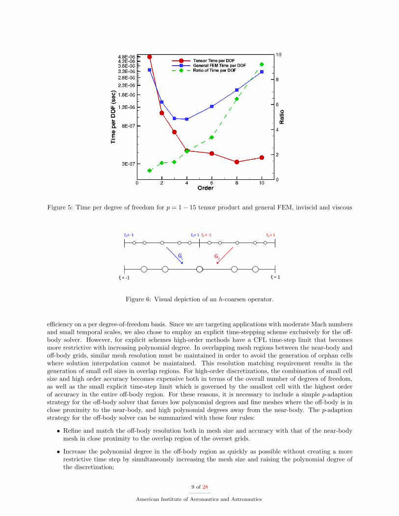
Figure 5: Time per degree of freedom for p = 1− 15 tensor product and general FEM, inviscid and viscous
G G1 2
ξ = -1 ξ = 1
ξ1= -1 ξ1= 1 ξ2 = -1 ξ2 = 1
Figure 6: Visual depiction of an h-coarsen operator.
efficiency on a per degree-of-freedom basis. Since we are targeting applications with moderate Mach numbersand small temporal scales, we also chose to employ an explicit time-stepping scheme exclusively for the off-body solver. However, for explicit schemes high-order methods have a CFL time-step limit that becomesmore restrictive with increasing polynomial degree. In overlapping mesh regions between the near-body andoff-body grids, similar mesh resolution must be maintained in order to avoid the generation of orphan cellswhere solution interpolation cannot be maintained. This resolution matching requirement results in thegeneration of small cell sizes in overlap regions. For high-order discretizations, the combination of small cellsize and high order accuracy becomes expensive both in terms of the overall number of degrees of freedom,as well as the small explicit time-step limit which is governed by the smallest cell with the highest orderof accuracy in the entire off-body region. For these reasons, it is necessary to include a simple p-adaptionstrategy for the off-body solver that favors low polynomial degrees and fine meshes where the off-body is inclose proximity to the near-body, and high polynomial degrees away from the near-body. The p-adaptionstrategy for the off-body solver can be summarized with these four rules:
• Refine and match the off-body resolution both in mesh size and accuracy with that of the near-bodymesh in close proximity to the overlap region of the overset grids.
• Increase the polynomial degree in the off-body region as quickly as possible without creating a morerestrictive time step by simultaneously increasing the mesh size and raising the polynomial degree ofthe discretization;
9 of 28
American Institute of Aeronautics and Astronautics
P P1 2
ξ = -1 ξ = 1
ξ1= -1 ξ1= 0 ξ2 = 0 ξ2 = 1
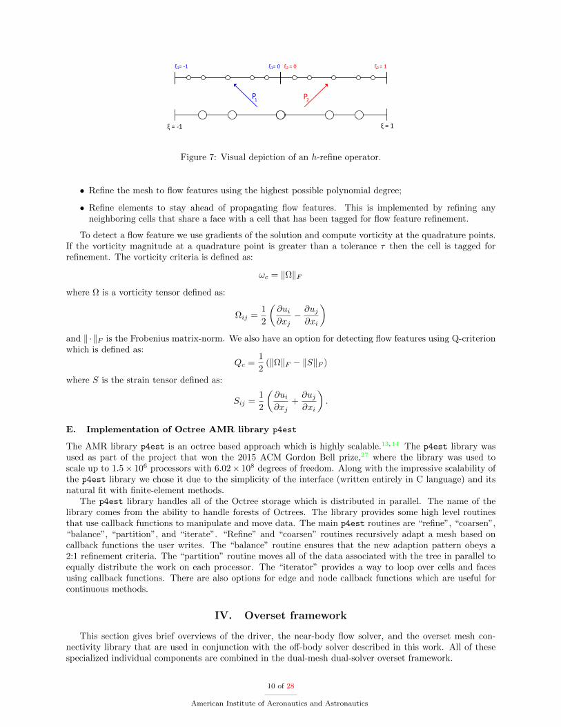
Figure 7: Visual depiction of an h-refine operator.
• Refine the mesh to flow features using the highest possible polynomial degree;
• Refine elements to stay ahead of propagating flow features. This is implemented by refining anyneighboring cells that share a face with a cell that has been tagged for flow feature refinement.
To detect a flow feature we use gradients of the solution and compute vorticity at the quadrature points.If the vorticity magnitude at a quadrature point is greater than a tolerance τ then the cell is tagged forrefinement. The vorticity criteria is defined as:
ωc = ‖Ω‖F
where Ω is a vorticity tensor defined as:
Ωij =1
2
(∂ui∂xj− ∂uj∂xi
)and ‖ ·‖F is the Frobenius matrix-norm. We also have an option for detecting flow features using Q-criterionwhich is defined as:
Qc =1
2(‖Ω‖F − ‖S‖F )
where S is the strain tensor defined as:
Sij =1
2
(∂ui∂xj
+∂uj∂xi
).
E. Implementation of Octree AMR library p4est
The AMR library p4est is an octree based approach which is highly scalable.13,14 The p4est library wasused as part of the project that won the 2015 ACM Gordon Bell prize,27 where the library was used toscale up to 1.5× 10⁶ processors with 6.02× 10⁸ degrees of freedom. Along with the impressive scalability ofthe p4est library we chose it due to the simplicity of the interface (written entirely in C language) and itsnatural fit with finite-element methods.
The p4est library handles all of the Octree storage which is distributed in parallel. The name of thelibrary comes from the ability to handle forests of Octrees. The library provides some high level routinesthat use callback functions to manipulate and move data. The main p4est routines are “refine”, “coarsen”,“balance”, “partition”, and “iterate”. “Refine” and “coarsen” routines recursively adapt a mesh based oncallback functions the user writes. The “balance” routine ensures that the new adaption pattern obeys a2:1 refinement criteria. The “partition” routine moves all of the data associated with the tree in parallel toequally distribute the work on each processor. The “iterator” provides a way to loop over cells and facesusing callback functions. There are also options for edge and node callback functions which are useful forcontinuous methods.
IV. Overset framework
This section gives brief overviews of the driver, the near-body flow solver, and the overset mesh con-nectivity library that are used in conjunction with the off-body solver described in this work. All of thesespecialized individual components are combined in the dual-mesh dual-solver overset framework.
10 of 28
American Institute of Aeronautics and Astronautics
A. Driver
In a multi-solver framework a main driving routine is needed to coordinate and run each individual solvercomponent. The driver in this work is similar to the multi-solver framework developed by Wissink et al.in Ref28 with some notable differences. In this previous work, a Python interface is used to dynamicallyload different solvers, where each individual flow solver is typically run in sequence across all processors.This has the advantage of automatically load balancing across solver types but has some disadvantages.Each flow solver has a different amount of computational work and scales differently and in many instancesconcurrent execution of the different solvers on the optimal number of processors results in more effectiveresource utilization. Also, high-order implicit solvers have a very large memory footprint and running eachsolver on the same group of processors may have significant implications for memory requirements.
The driver in this work is written in C, handles multiple coding languages (C, C++, and Fortran) inthe component solvers, and performs parallel communication through MPI. It has the flexibility of runningflow-solvers sequentially on the same set of processors or concurrently on different processor groups. Thesolvers used in this work are self contained and only communicate with each other through the TIOGAoverset mesh assembler. TIOGA performs both implicit hole cutting on all meshes and executes the fringecell interpolation between overlapping meshes. All flow solvers and other codes that are controlled by thedriver will be referred to as modules. These modules can include near-body and off-body flow solvers,overset domain connectivity assemblers, as well as other disciplinary solvers such as structural solvers, meshdeformation solvers, and even atmospheric boundary layer solvers to provide turbulent inflow conditions forwind turbine simulations.7,29
B. Unstructured near-body finite volume solver: NSU3D
NSU3D is an unstructured mesh multigrid Unsteady Reynolds-averaged Navier-Stokes (URANS) solverdeveloped for high-Reynolds number external aerodynamic applications. NSU3D employs a second-orderaccurate vertex-based discretization, where the unknown fluid and turbulence variables are stored at thevertices of the mesh, and fluxes are computed on faces delimiting dual control volumes, with each dualface being associated with a mesh edge. This discretization operates on hybrid mixed-element meshes,generally employing prismatic elements in highly stretched boundary layer regions, and tetrahedral elementsin isotropic regions of the mesh. A single edge-based data structure is used to compute flux balances acrossall types of elements. The single-equation Spalart-Allmaras turbulence model30 as well as a standard k − ωtwo-equation turbulence model31 are available within the NSU3D solver.
The NSU3D solution scheme was originally developed for optimizing convergence of steady-state prob-lems. The basic approach relies on an explicit multistage scheme which is preconditioned by a local block-Jacobi preconditioner in regions of isotropic grid cells. In boundary layer regions, where the grid is highlystretched, a line preconditioner is employed to relieve the stiffness associated with the mesh anisotropy.32 Anagglomeration multigrid algorithm is used to further enhance convergence to steady-state.33,34 The Jacobiand line preconditioners are used to drive the various levels of the multigrid sequence, resulting in a rapidlyconverging solution technique.
For time-dependent problems, a second-order implicit backwards difference time discretization is em-ployed, and the line-implicit multigrid scheme is used to solve the non-linear problem arising at each implicittime step. NSU3D has been extensively validated in stand-alone mode, both for steady-state fixed-wingcases, as a regular participant in the AIAA Drag Prediction workshop series,35 as well as for unsteadyaerodynamic and aeroelastic problems,36 and has been benchmarked on large parallel computer systems.37
C. Overset Mesh Assembly: TIOGA
The overset grid connectivities are handled through the TIOGA interface (Topology Independent OversetGrid Assembler).38 The TIOGA overset grid assembler relies on an efficient parallel implementation ofAlternating Digital Trees (ADT)39 for point-cell inclusion tests. Multiple grids are loaded in parallel andTIOGA computes the IBLANKing information required by the flow solver, as well as the cell donor-receptorinformation. We use the notation IBLANK which is an array of integers used to identify cell type in theoverset framework. In this notation a fringe cell has IBLANK value of: IBLANK = −1, a hole cell: IBLANK= 0, and a field cell: IBLANK = 1. A hole cell occurs when an outer mesh overlaps an inner mesh with anenclosed surface (such as a geometry component). This hole cell does not contain a donor cell and is usuallyeliminated from the discretization. This is allowed because a collection of hole cells needs to be completely
11 of 28
American Institute of Aeronautics and Astronautics
surrounded by fringe cells. This in turn means that the field cells only interact with fringe cells. If a fieldcell neighbors a hole cell then the overset connectivity fails. In order to interface TIOGA with a high-ordermethod several callback functions need to be supplied. This allows high-order interpolation which is requiredto maintain overall high-order solution accuracy.10
V. Results
There are four sets of results that demonstrate the performance, efficiency, and capability of the DG AMRsolver. The first two consist of the simulations of Ringleb flow and the Taylor-Green vortex to test the stand-alone capabilities. The last two utilize overset meshes and are solved in conjunction with a finite-volumenear-body solver NSU3D for flow over a NACA 0015 wing and a NREL PhaseVI wind turbine.
A. Ringleb flow mesh resolution study
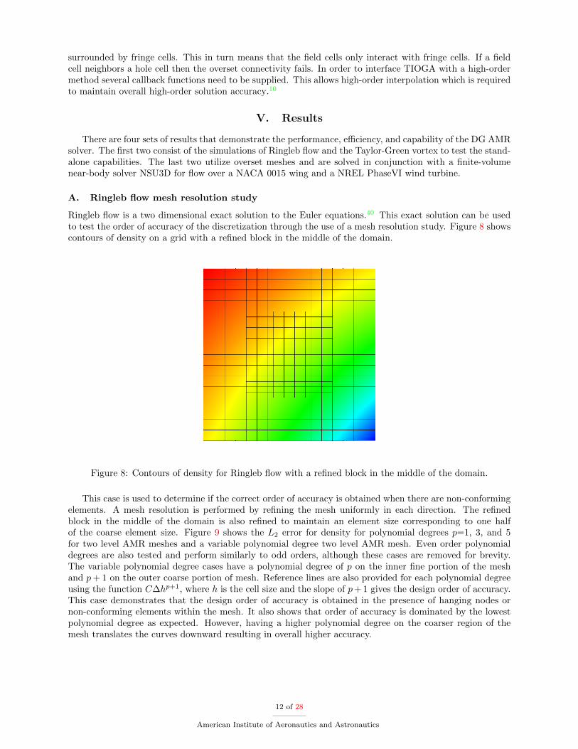
Ringleb flow is a two dimensional exact solution to the Euler equations.40 This exact solution can be usedto test the order of accuracy of the discretization through the use of a mesh resolution study. Figure 8 showscontours of density on a grid with a refined block in the middle of the domain.
Figure 8: Contours of density for Ringleb flow with a refined block in the middle of the domain.
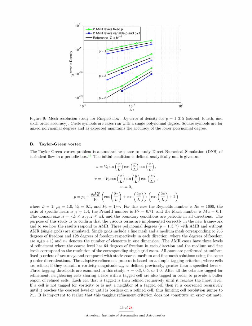
This case is used to determine if the correct order of accuracy is obtained when there are non-conformingelements. A mesh resolution is performed by refining the mesh uniformly in each direction. The refinedblock in the middle of the domain is also refined to maintain an element size corresponding to one halfof the coarse element size. Figure 9 shows the L2 error for density for polynomial degrees p=1, 3, and 5for two level AMR meshes and a variable polynomial degree two level AMR mesh. Even order polynomialdegrees are also tested and perform similarly to odd orders, although these cases are removed for brevity.The variable polynomial degree cases have a polynomial degree of p on the inner fine portion of the meshand p+ 1 on the outer coarse portion of mesh. Reference lines are also provided for each polynomial degreeusing the function C∆hp+1, where h is the cell size and the slope of p+ 1 gives the design order of accuracy.This case demonstrates that the design order of accuracy is obtained in the presence of hanging nodes ornon-conforming elements within the mesh. It also shows that order of accuracy is dominated by the lowestpolynomial degree as expected. However, having a higher polynomial degree on the coarser region of themesh translates the curves downward resulting in overall higher accuracy.
12 of 28
American Institute of Aeronautics and Astronautics
10−2
10−1
100
10−15
10−10
10−5
100
∆ x
L2 e
rro
r in
De
nsity
p = 1
p = 3
p = 5
2 AMR levels fixed p
2 AMR levels variable p and p+1
Reference C ∆ hp+1
Figure 9: Mesh resolution study for Ringleb flow. L2 error of density for p = 1, 3, 5 (second, fourth, andsixth order accuracy). Circle symbols are cases run with a single polynomial degree. Square symbols are formixed polynomial degrees and as expected maintains the accuracy of the lower polynomial degree.
B. Taylor-Green vortex
The Taylor-Green vortex problem is a standard test case to study Direct Numerical Simulation (DNS) ofturbulent flow in a periodic box.41 The initial condition is defined analytically and is given as:
u = V0 sin( xL
)cos( yL
)cos( zL
),
v = −V0 cos( xL
)sin( yL
)cos( zL
),
w = 0,
p = p0 +ρ0V
20
16
(cos
(2x
L
)+ cos
(2y
L
))(cos
(2z
L
)+ 2
)where L = 1, ρ0 = 1.0, V0 = 0.1, and P0 = 1/γ. For this case the Reynolds number is Re = 1600, theratio of specific heats is γ = 1.4, the Prandtl number is Pr = 0.71, and the Mach number is Ma = 0.1.The domain size is = πL ≤ x, y, z ≤ πL and the boundary conditions are periodic in all directions. Thepurpose of this study is to confirm that the viscous terms are implemented correctly in the new frameworkand to see how the results respond to AMR. Three polynomial degrees (p = 1, 3, 7) with AMR and withoutAMR (single grids) are simulated. Single grids include a fine mesh and a medium mesh corresponding to 256degrees of freedom and 128 degrees of freedom respectively in each direction, where the degrees of freedomare ne(p + 1) and ne denotes the number of elements in one dimension. The AMR cases have three levelsof refinement where the coarse level has 64 degrees of freedom in each direction and the medium and finelevels correspond to the resolution of the corresponding single grid cases. All cases are performed at uniformfixed p-orders of accuracy, and compared with static coarse, medium and fine mesh solutions using the samep-order discretizations. The adaptive refinement process is based on a simple tagging criterion, where cellsare refined if they contain a vorticity magnitude ωc, as defined previously, greater than a specified level τ .Three tagging thresholds are examined in this study: τ = 0.3, 0.5, or 1.0. After all the cells are tagged forrefinement, neighboring cells sharing a face with a tagged cell are also tagged in order to provide a bufferregion of refined cells. Each cell that is tagged is then refined recursively until it reaches the finest level.If a cell is not tagged for vorticity or is not a neighbor of a tagged cell then it is coarsened recursivelyuntil it reaches the coarsest level or until is borders on a refined cell, thus limiting cell resolution jumps to2:1. It is important to realize that this tagging refinement criterion does not constitute an error estimate.
13 of 28
American Institute of Aeronautics and Astronautics
Rather we follow this simple feature-based approach which has proven to be successful for capturing vorticalstructures for rotorcraft and wind energy problems particularly in the HELIOS software framework,42 withthe understanding that a more fundamental error-based approach should be considered in future work.
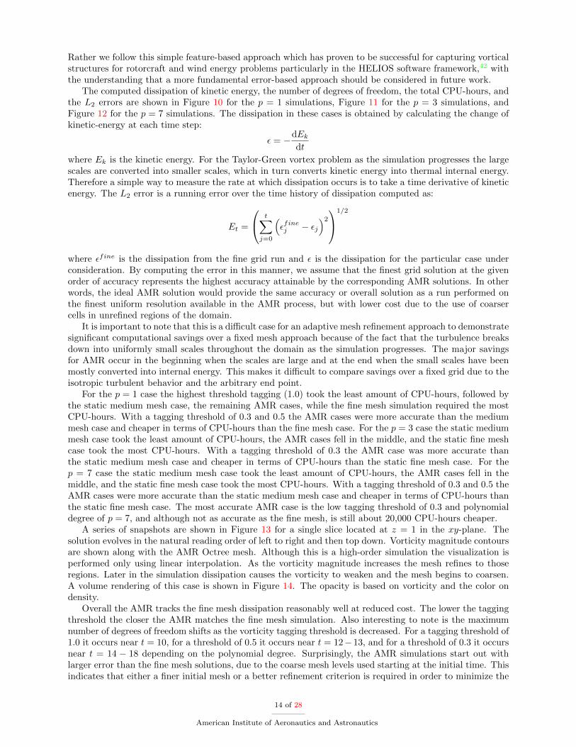
The computed dissipation of kinetic energy, the number of degrees of freedom, the total CPU-hours, andthe L2 errors are shown in Figure 10 for the p = 1 simulations, Figure 11 for the p = 3 simulations, andFigure 12 for the p = 7 simulations. The dissipation in these cases is obtained by calculating the change ofkinetic-energy at each time step:
ε = −dEk
dt
where Ek is the kinetic energy. For the Taylor-Green vortex problem as the simulation progresses the largescales are converted into smaller scales, which in turn converts kinetic energy into thermal internal energy.Therefore a simple way to measure the rate at which dissipation occurs is to take a time derivative of kineticenergy. The L2 error is a running error over the time history of dissipation computed as:
Et =
t∑j=0
(εfinej − εj
)2
1/2
where εfine is the dissipation from the fine grid run and ε is the dissipation for the particular case underconsideration. By computing the error in this manner, we assume that the finest grid solution at the givenorder of accuracy represents the highest accuracy attainable by the corresponding AMR solutions. In otherwords, the ideal AMR solution would provide the same accuracy or overall solution as a run performed onthe finest uniform resolution available in the AMR process, but with lower cost due to the use of coarsercells in unrefined regions of the domain.
It is important to note that this is a difficult case for an adaptive mesh refinement approach to demonstratesignificant computational savings over a fixed mesh approach because of the fact that the turbulence breaksdown into uniformly small scales throughout the domain as the simulation progresses. The major savingsfor AMR occur in the beginning when the scales are large and at the end when the small scales have beenmostly converted into internal energy. This makes it difficult to compare savings over a fixed grid due to theisotropic turbulent behavior and the arbitrary end point.
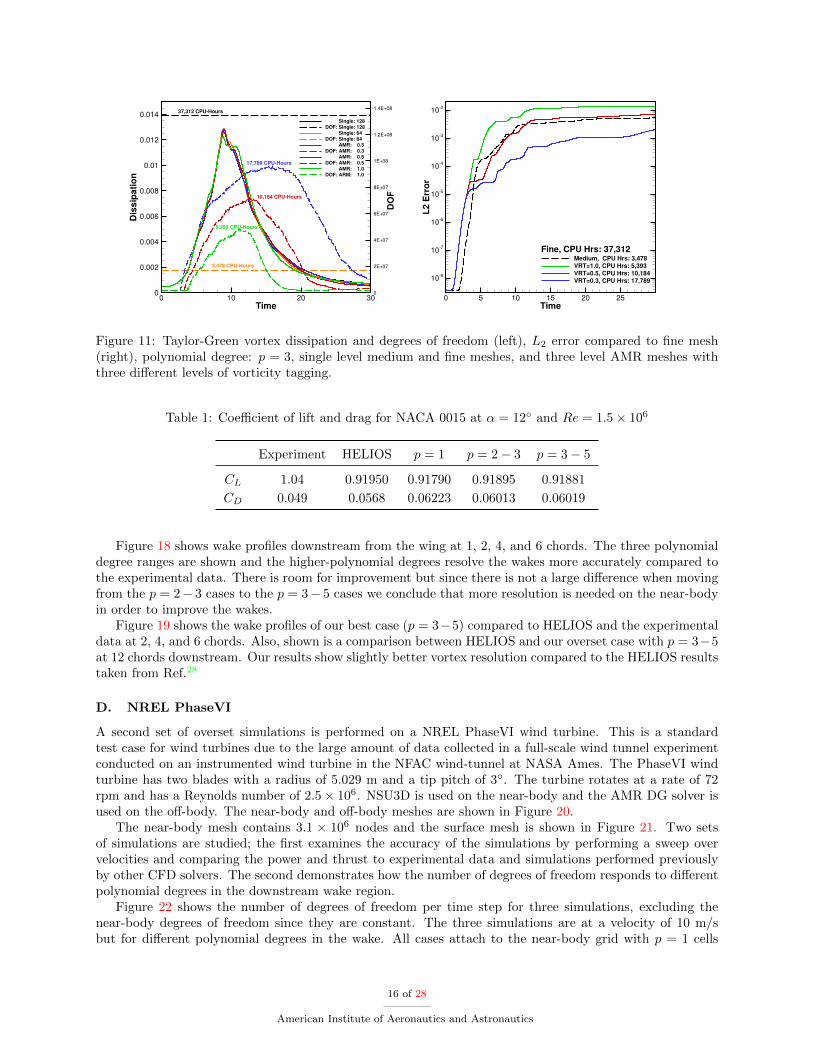
For the p = 1 case the highest threshold tagging (1.0) took the least amount of CPU-hours, followed bythe static medium mesh case, the remaining AMR cases, while the fine mesh simulation required the mostCPU-hours. With a tagging threshold of 0.3 and 0.5 the AMR cases were more accurate than the mediummesh case and cheaper in terms of CPU-hours than the fine mesh case. For the p = 3 case the static mediummesh case took the least amount of CPU-hours, the AMR cases fell in the middle, and the static fine meshcase took the most CPU-hours. With a tagging threshold of 0.3 the AMR case was more accurate thanthe static medium mesh case and cheaper in terms of CPU-hours than the static fine mesh case. For thep = 7 case the static medium mesh case took the least amount of CPU-hours, the AMR cases fell in themiddle, and the static fine mesh case took the most CPU-hours. With a tagging threshold of 0.3 and 0.5 theAMR cases were more accurate than the static medium mesh case and cheaper in terms of CPU-hours thanthe static fine mesh case. The most accurate AMR case is the low tagging threshold of 0.3 and polynomialdegree of p = 7, and although not as accurate as the fine mesh, is still about 20,000 CPU-hours cheaper.
A series of snapshots are shown in Figure 13 for a single slice located at z = 1 in the xy-plane. Thesolution evolves in the natural reading order of left to right and then top down. Vorticity magnitude contoursare shown along with the AMR Octree mesh. Although this is a high-order simulation the visualization isperformed only using linear interpolation. As the vorticity magnitude increases the mesh refines to thoseregions. Later in the simulation dissipation causes the vorticity to weaken and the mesh begins to coarsen.A volume rendering of this case is shown in Figure 14. The opacity is based on vorticity and the color ondensity.
Overall the AMR tracks the fine mesh dissipation reasonably well at reduced cost. The lower the taggingthreshold the closer the AMR matches the fine mesh simulation. Also interesting to note is the maximumnumber of degrees of freedom shifts as the vorticity tagging threshold is decreased. For a tagging threshold of1.0 it occurs near t = 10, for a threshold of 0.5 it occurs near t = 12− 13, and for a threshold of 0.3 it occursnear t = 14 − 18 depending on the polynomial degree. Surprisingly, the AMR simulations start out withlarger error than the fine mesh solutions, due to the coarse mesh levels used starting at the initial time. Thisindicates that either a finer initial mesh or a better refinement criterion is required in order to minimize the
14 of 28
American Institute of Aeronautics and Astronautics
Time
Dis
sip
ati
on
DO
F
0 10 20 300
0.002
0.004
0.006
0.008
0.01
0.012
0.014
0
2E+07
4E+07
6E+07
8E+07
1E+08
1.2E+08
1.4E+08
Single: 256
DOF: Single: 256 Single: 128
DOF: Single: 128
AMR: 0.3
DOF: AMR: 0.3
AMR: 0.5
DOF: AMR: 0.5
AMR: 1.0
DOF: ARM: 1.0
19,102 CPUHours
10,125 CPUHours
4,675 CPUHours
5,339 CPUHours
1,871 CPUHours
Time
L2
Err
or
5 10 15 20 25
105
104
103
102
Medium, CPU Hrs: 5,339
VRT=1.0, CPU Hrs: 1,871
VRT=0.5, CPU Hrs: 4,675
VRT=0.3, CPU Hrs: 10,125
Fine, CPU Hrs: 19,102
Figure 10: Taylor-Green vortex dissipation and degrees of freedom (left), L2 error compared to fine mesh(right), polynomial degree: p = 1, single level medium and fine meshes, and three level AMR meshes withthree different levels of vorticity tagging.
error at the initial times of the simulation. Additionally, the relative efficiency of the AMR cases comparedto the static mesh cases improves for longer simulation times, due to the additional dissipation of the smallestscales for longer simulation times.
C. NACA 0015 wing
The first overset simulation consists of the study of flow over a wing based on a NACA 0015 airfoil. TheNACA 0015 wing has been studied experimentally by McAlister and Takhashi.43 Computational studieshave been performed by Wissink,42 Sitaraman and Baeder,44 and by Hariharan and Sankar.45
For this case we demonstrate the capability of simulating unsteady, turbulent flow over a rectangularsquare-tipped lifting wing. The wing is based on a constant cross-section NACA0015 airfoil, and has a finitespan of 6.6 chords. For this case the Mach number is 0.1235, the angle of attack is α = 12, and the Reynoldsnumber is 1.5 million (based on chord length c).
NSU3D is used on the near-body solver and the AMR DG solver is used on the off-body solver. The oversetmesh configuration is shown in Figure 15. This case is used to demonstrate the ability to combine a node-based finite-volume discretization with a cell-based, high-order, DG discretization in an overset framework,and to accurately capture wing-tip vortices. NSU3D solves the unsteady RANS equations closed by theSpalart-Allmaras with Rotation Correction (SA-RC) turbulence model.46 NSU3D employs a steady-stateimplicit solver on a mesh with 4.4 × 10⁶ nodes. The off-body AMR solver runs explicitly with RK4 at anon-dimensional time step of ∆tu∞/c = 0.036. Figure 16 shows iso-contours of vorticity equal to 1.0 and3.0 and slices of AMR grids all the way to a location 48 chords downstream.
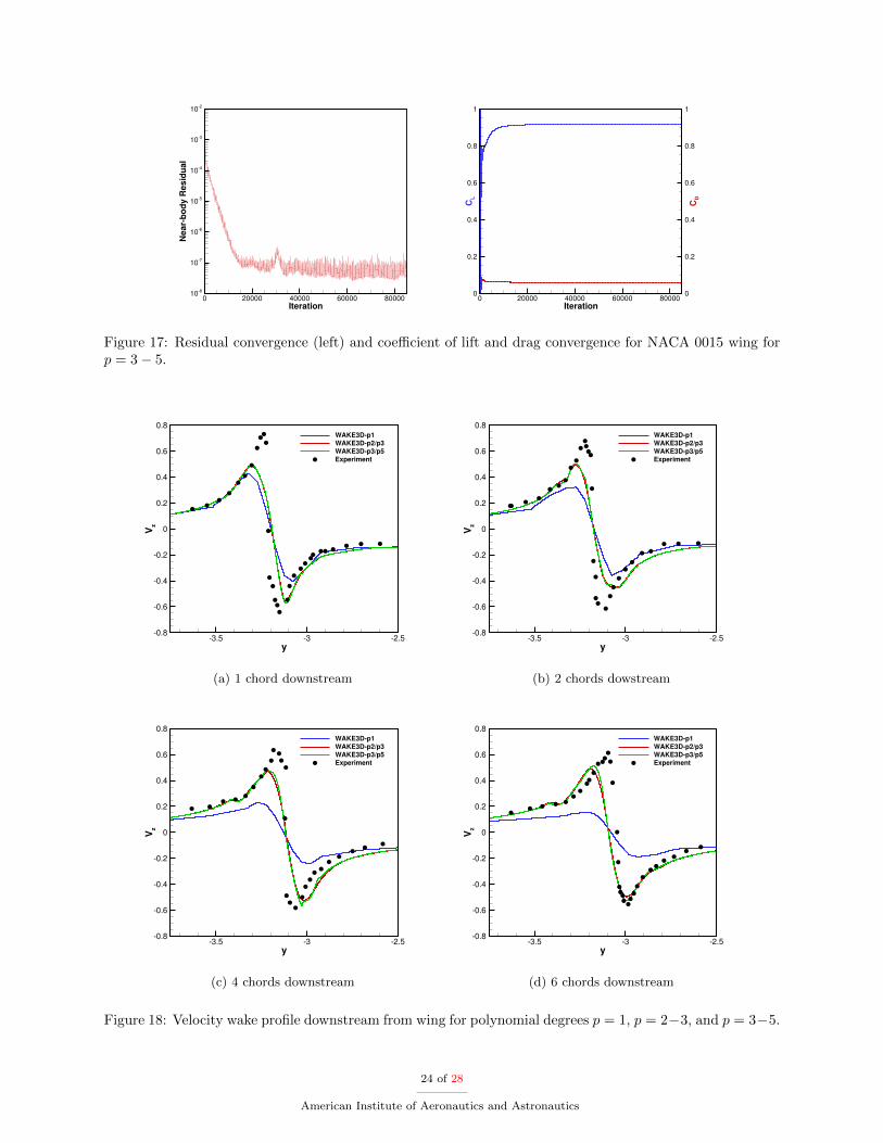
Three ranges of polynomial degrees are studied in this case for the off-body DG discretization. The firstis uniform p = 1, the second is p = 2 to attach to the near-body and p = 3 in the wake, and the third isp = 3 to attach to the near-body and grows to p = 5 in the wake. Off-body refinement occurs when vorticitymagnitude wc is greater than a tolerance of τ = 0.4. The non-linear residual convergence and lift and dragcoefficients are shown in Figure 17 for only the p = 3− 5 case but show similar trends to the other cases. Aresidual reduction of four orders of magnitude for the near-body solver is obtained although full convergenceto steady-state is inhibited due to the time dependent nature of the off-body flow solver. The lift and dragtime histories exhibit small oscillations and a moving average with a window of 10,000 non-linear near-bodysolution updates is used to estimate the lift and drag as shown inTable 1.
The lift and drag for each of these cases shown in Table 1 are also compared to experimental data43 andHELIOS simulation results taken from Ref.28 The HELIOS simulations used the same near-body resolutionas the current results. HELIOS has improved these results recently47,48 but at the same time modified thenear-body mesh so we compare to HELIOS results from Ref.28
15 of 28
American Institute of Aeronautics and Astronautics
Time
Dis
sip
ati
on
DO
F
0 10 20 300
0.002
0.004
0.006
0.008
0.01
0.012
0.014
0
2E+07
4E+07
6E+07
8E+07
1E+08
1.2E+08
1.4E+08
Single: 128
DOF: Single: 128 Single: 64
DOF: Single: 64
AMR: 0.3
DOF: AMR: 0.3
AMR: 0.5
DOF: AMR: 0.5
AMR: 1.0
DOF: ARM: 1.0
37,312 CPUHours
17,789 CPUHours
10,184 CPUHours
3,478 CPUHours
5,393 CPUHours
Time
L2
Err
or
0 5 10 15 20 25
108
107
106
105
104
103
102
Medium, CPU Hrs: 3,478
VRT=1.0, CPU Hrs: 5,393
VRT=0.5, CPU Hrs: 10,184
VRT=0.3, CPU Hrs: 17,789
Fine, CPU Hrs: 37,312
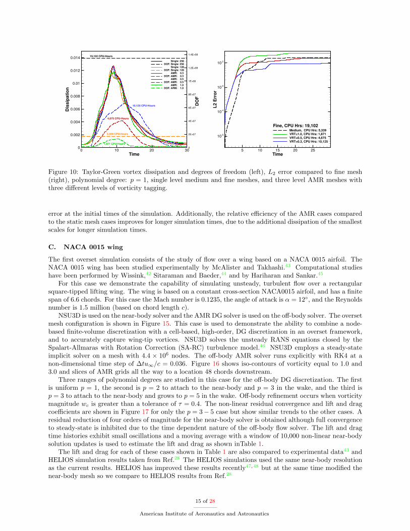
Figure 11: Taylor-Green vortex dissipation and degrees of freedom (left), L2 error compared to fine mesh(right), polynomial degree: p = 3, single level medium and fine meshes, and three level AMR meshes withthree different levels of vorticity tagging.
Table 1: Coefficient of lift and drag for NACA 0015 at α = 12 and Re = 1.5× 10⁶
Experiment HELIOS p = 1 p = 2− 3 p = 3− 5
CL 1.04 0.91950 0.91790 0.91895 0.91881
CD 0.049 0.0568 0.06223 0.06013 0.06019
Figure 18 shows wake profiles downstream from the wing at 1, 2, 4, and 6 chords. The three polynomialdegree ranges are shown and the higher-polynomial degrees resolve the wakes more accurately compared tothe experimental data. There is room for improvement but since there is not a large difference when movingfrom the p = 2− 3 cases to the p = 3− 5 cases we conclude that more resolution is needed on the near-bodyin order to improve the wakes.
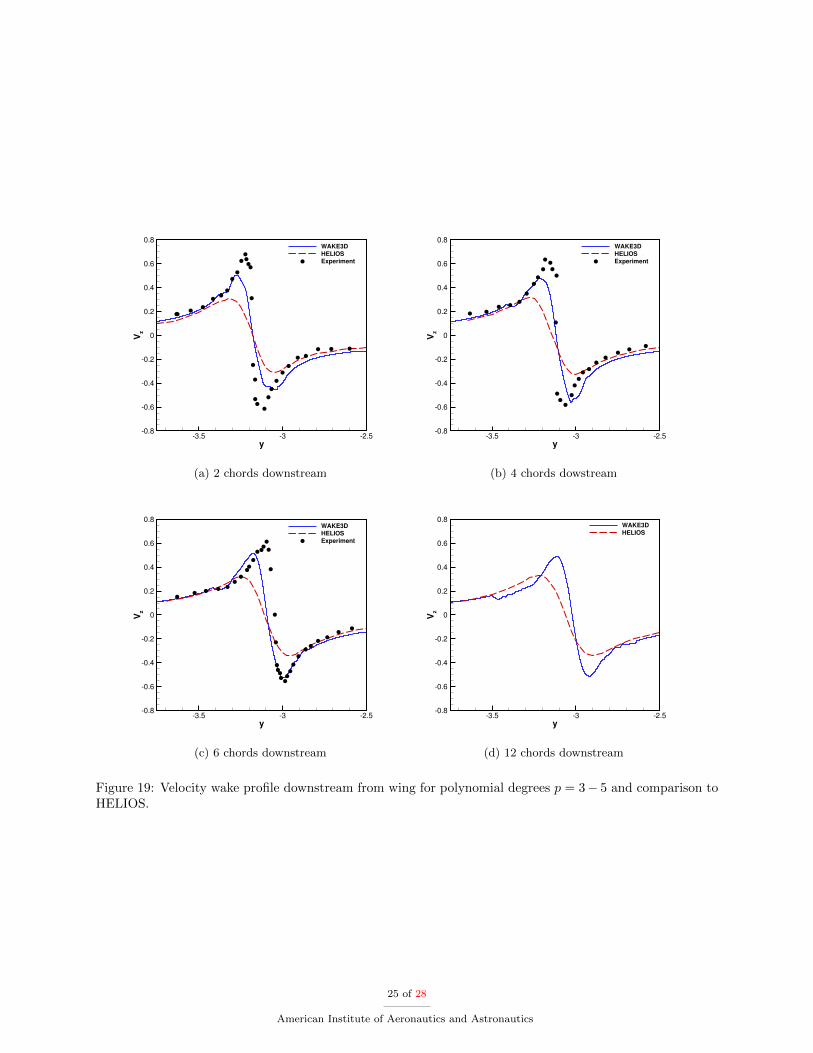
Figure 19 shows the wake profiles of our best case (p = 3−5) compared to HELIOS and the experimentaldata at 2, 4, and 6 chords. Also, shown is a comparison between HELIOS and our overset case with p = 3−5at 12 chords downstream. Our results show slightly better vortex resolution compared to the HELIOS resultstaken from Ref.28
D. NREL PhaseVI
A second set of overset simulations is performed on a NREL PhaseVI wind turbine. This is a standardtest case for wind turbines due to the large amount of data collected in a full-scale wind tunnel experimentconducted on an instrumented wind turbine in the NFAC wind-tunnel at NASA Ames. The PhaseVI windturbine has two blades with a radius of 5.029 m and a tip pitch of 3. The turbine rotates at a rate of 72rpm and has a Reynolds number of 2.5× 10⁶. NSU3D is used on the near-body and the AMR DG solver isused on the off-body. The near-body and off-body meshes are shown in Figure 20.
The near-body mesh contains 3.1 × 10⁶ nodes and the surface mesh is shown in Figure 21. Two setsof simulations are studied; the first examines the accuracy of the simulations by performing a sweep overvelocities and comparing the power and thrust to experimental data and simulations performed previouslyby other CFD solvers. The second demonstrates how the number of degrees of freedom responds to differentpolynomial degrees in the downstream wake region.
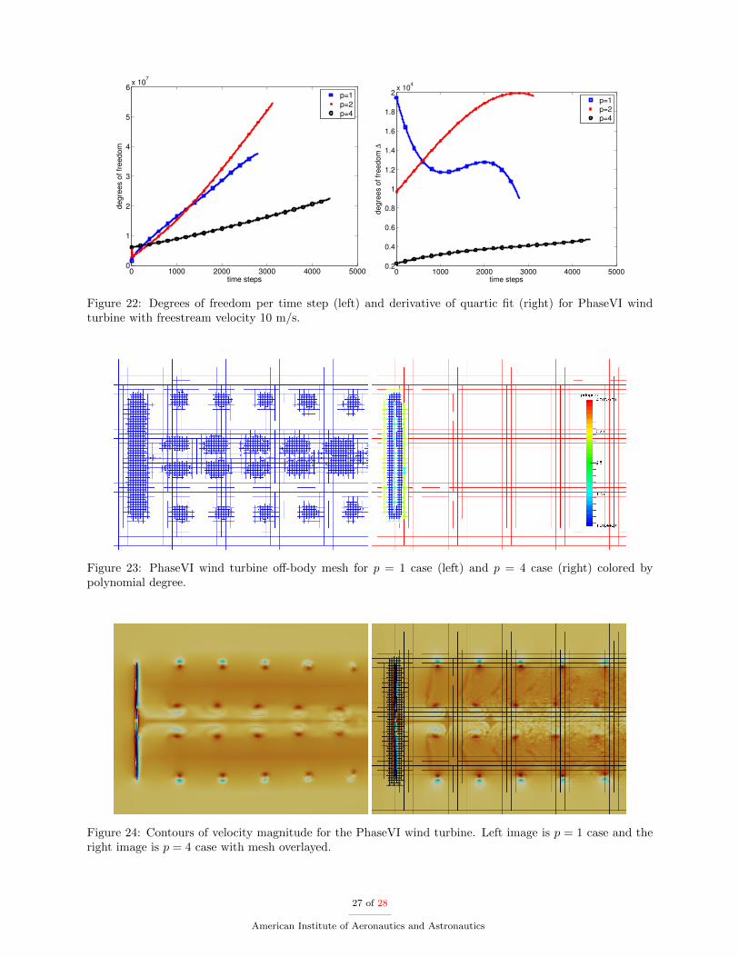
Figure 22 shows the number of degrees of freedom per time step for three simulations, excluding thenear-body degrees of freedom since they are constant. The three simulations are at a velocity of 10 m/sbut for different polynomial degrees in the wake. All cases attach to the near-body grid with p = 1 cells
16 of 28
American Institute of Aeronautics and Astronautics
Time
Dis
sip
ati
on
DO
F
0 10 20 300
0.002
0.004
0.006
0.008
0.01
0.012
0.014
0
2E+07
4E+07
6E+07
8E+07
1E+08
1.2E+08
1.4E+08
Single: 64
DOF: Single: 64
Single: 32
DOF: Single: 32
AMR: 0.3
DOF: AMR: 0.3
AMR: 0.5
DOF: AMR: 0.5
AMR: 1.0
DOF: ARM: 1.0
119,752 CPUHours
98,083 CPUHours
64,795 CPUHours
12,341 CPUHours
39,565 CPUHours
Time
L2
Err
or
0 5 10 15 20 25
108
107
106
105
104
103
102
Medium, CPU Hrs: 12,341
VRT=1.0, CPU Hrs: 39,565
VRT=0.5, CPU Hrs: 64,795
VRT=0.3, CPU Hrs: 98,083
Fine, CPU Hrs: 119,752
Figure 12: Taylor-Green vortex dissipation and degrees of freedom (left), L2 error compared to fine mesh(right), polynomial degree: p = 7, single level medium and fine meshes, and three level AMR meshes withthree different levels of vorticity tagging.
and the polynomial degree grows to p = 1, 2, or 4. In the wake region a base mesh consisting of 5 levelsof refinement accounts for the relatively large number of degrees of freedom seen in the p = 4 case in thebeginning of the simulation. This can be ignored since we are more interested in the increase of degrees offreedom or the rate of change created as the wake of the wind turbine convects downstream. All cases arerun for 24 hours of wall-clock time on 576 cores (256 near-body and 320 off-body flow solver cores) and overthat time frame more time steps are obtained for the p = 4 solution compared to the cases run with lowerpolynomial degrees. Also, the p = 2 case exhibits a similar trend and more time steps are obtained comparedto the p = 1 case. More time steps are achieved for the higher polynomial degrees for two main reasons.The first is that the computational time per degree of freedom goes down slightly for higher polynomialdegrees. Additionally, the increase in degrees of freedom is greater for the lower polynomial degrees. Thismay not hold if the simulation was continued further because there is a cross over point with p = 1 and p = 2near time step 1300. To better understand these results a quartic polynomial is fitted to each case and thederivative of that polynomial is shown in Figure 22(b). This helps explain how the degrees of freedom areadded to the simulation over time. For the p = 1 case the number of degrees of freedom is always increasingalbeit more slowly over time. This could occur due to the wake dissipating over time and loss of resolutiondownstream from the turbine. The p = 2 case shows an opposite trend and the number of elements increasemore rapidly than linearly until near the end of the simulation. The p = 4 case is also growing quicker thanlinearly but at a more reasonable increase. These results are qualitative in nature, and a more quantitativestudy is required to determine the accuracy for each case and to determine whether the decrease in degreesof freedom but increase in polynomial degree results in a more accurate simulation.
Figure 23 shows the off-body mesh used for the p = 1 case and the p = 4 case. The mesh is colored usingpolynomial degree and the p = 4 case only uses p = 1 − 3 polynomial degrees close to the near-body. Thep = 1 case requires more cells to capture and track the wake compared to the p = 4 case. More cells in theoff-body puts a burden on both the p4est library and the overset connectivity library TIOGA. Figure 24shows contours of velocity magnitude for the p = 1 case and the p = 4 case with the mesh over-layed. Thep = 1 wake remains stable as the dissipation keeps the vortices from breaking down. The wake in the p = 4case breaks down into smaller scales. The plotting resolution on the p = 4 case is not fine enough to resolvethe solution in each cell since we only plot (p+ 1)d points in each cell.
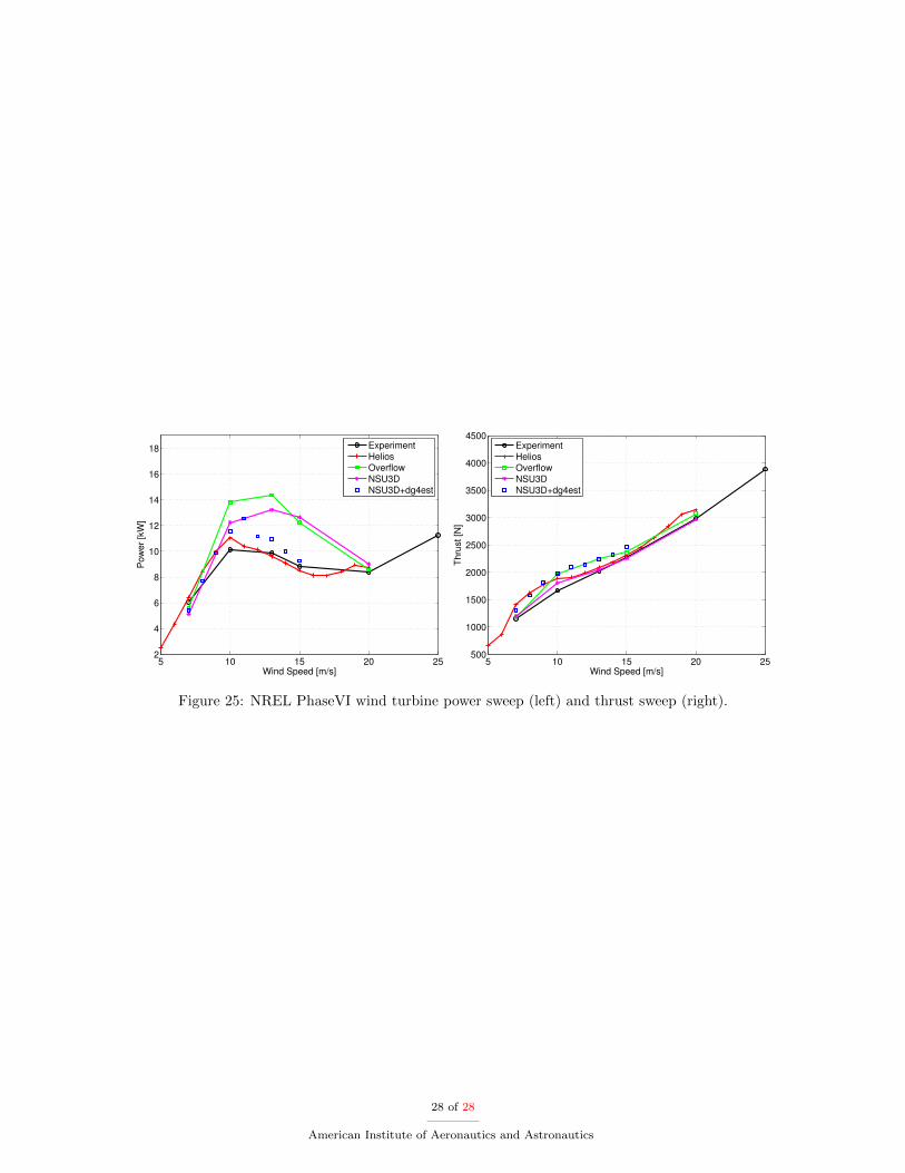
To test the accuracy of the overset framework, 9 simulations are carried out with varying free-streamvelocity. The off-body mesh uses a polynomial degree of p = 1 to attach to the near-body mesh and p = 4in the wake. The domain size is 1000 meters in each direction and contains 10 Octrees in each direction anda maximum of 11 levels of refinement. The maximum level of refinement is only used in the p = 1 regionwhile a maximum level of 8 is used in the p = 4 wake region. We study velocities 7 m/s to 15 m/s and reportintegrated forces. After 8 rotor revolutions of the wind turbine the forces are averaged and post processed to
17 of 28
American Institute of Aeronautics and Astronautics
obtain power and thrust. These are shown in Figure 25 and compared to experimental data and previouslyreported computational results.49 Good agreement is seen for velocities 7-10 m/s for all flow solvers andexperimental data. For velocities 11-15 m/s our overset results appear to delay blade stalling compared tothe HELIOS results and the experiment. Power in this range is overpredicted by approximately 10-20%,however our overset results are significantly more accurate than the stand-alone Overflow and NSU3D results.Conversely, thrust in the 11-15 m/s range is overpredicted by about 10%, which is similar to the Overflowresults.
VI. Conclusions
In this work we have developed a high-order off-body DG AMR solver. This solver uses an Octreebased AMR library called p4est which provides h-adaption capabilities. In addition the DG AMR solverincorporates a p-refinement capability which allows each cell to have a variable polynomial degree. Thecombined hp-refinement strategy allows for a highly efficient off-body solver for use in an overset framework.We have demonstrated the feasibility, accuracy, and capabilities of this off-body solver on two stand-alonecases which include Ringleb flow and Taylor-Green vortex. Also, we have demonstrated the ability to simulatetwo overset simulations. The first is a static overset NACA 0015 wing which compares well to experimentalresults and HELIOS. The second is a dynamic overset simulation of a PhaseVI wind turbine. Both of theseoverset cases show the added benefit of incorporating high-order accuracy in the off-body solver by increasingthe accuracy and efficiency of the overall overset framework. Future work will focus on the development ofan error-based refinement criterion for combined hp-refinement in wake regions and the validation of thisapproach for LES type simulations.
VII. Acknowledgments
This work was supported in part by ONR Grants N00014-14-1-0045 and N00014-16-1-2737 and by the U.S.Department of Energy, Office of Science, Basic Energy Sciences, under Award DE-SC0012671. Computertime was provided by the NCAR-Wyoming Supercomputing Center (NWSC) and University of WyomingAdvanced Research Computing Center (ARCC). The second author was supported in part by the NSF BlueWaters Graduate Fellowship as part of the Blue Waters sustained-petascale computing project, which issupported by the National Science Foundation (awards OCI-0725070 and ACI-1238993).
18 of 28
American Institute of Aeronautics and Astronautics
References
1Murphy, K. J., Buning, P. G., Pamadi, B. N., Scallion, W. I., and Jones, K. M., “Overview of Transonic to HypersonicStage Separation Tool Development for Multi-Stage-To-Orbit Concepts,” AIAA Paper 2004-2595 .
2Brown, D. L. and Henshaw, W. D., “Overture: An Object-Oriented Framework for Solving Partial Differential Equationson Overlapping Grids,” Object Oriented Methods for Interoperable Scientific and Engineering Computing, SIAM , 1999, pp. 245–255.
3Noack, R., “SUGGAR: a general capability for moving body overset grid assembly,” AIAA paper 2005-5117 .4Wissink, A., Kamkar, S., Pulliam, T., Sitaraman, J., and Sankaran, V., “Cartesian Adaptive Mesh Refinement for
Rotorcraft Wake Resolution,” AIAA, 28th Applied Aerodynamics Conference, 2010, AIAA Paper 2010-4554, 28th AIAA AppliedAerodynamics Conference, Chicago, IL, June 2010.
5Buning, P. G., Gomez, R. J., and Scallion, W. I., “CFD Approaches for Simulation of Wing-Body Stage Separation,”AIAA Paper 2004-4838 .
6Biedron, R. T. and Thomas, J. L., “Recent Enhancements to the FUN3D Flow Solver for Moving-Mesh Applications,”AIAA Paper 2009-1360 .
7Sitaraman, J., Mavriplis, D. J., and Duque, E. P., “Wind Farm simulations using a Full Rotor Model for Wind Turbines,”AIAA Paper 2014-1086 , 2015/05/29 2014.
8Sankaran, V., Sitaraman, J., Wissink, A., Datta, A., Jayaraman, B., Potsdam, M., Mavriplis, D., Yang, Z., O’Brien, D.,Saberi, H., et al., “Application of the Helios Computational Platform to Rotorcraft Flowfields,” AIAA paper 2010-1230 .
9Galbraith, M. C., Benek, J. A., Orkwis, P. D., and Turner, M. G., “A Discontinuous Galerkin Chimera scheme,”Computers & Fluids, Vol. 98, No. 0, 2014, pp. 27 – 53.
10Brazell, M. J., Sitaraman, J., and Mavriplis, D. J., “An overset mesh approach for 3D mixed element high-order dis-cretizations,” Journal of Computational Physics, Vol. 322, 10 2016, pp. 33–51.
11Zhang, B. and Liang, C., “A Simple, Efficient, High-Order Accurate Sliding-mesh Interface Approach to FR/CPR Methodon Coupled Rotating and Stationary Domains,” AIAA Paper 2015-1742 , 2015/06/01 2015.
12Merrill, B. E., Peet, Y. T., Fischer, P. F., and Lottes, J. W., “A spectrally accurate method for overlapping grid solutionof incompressible Navier–Stokes equations,” Journal of Computational Physics, Vol. 307, 2 2016, pp. 60–93.
13Burstedde, C., Wilcox, L. C., and Ghattas, O., “p4est: Scalable Algorithms for Parallel Adaptive Mesh Refinement onForests of Octrees,” SIAM Journal on Scientific Computing, Vol. 33, No. 3, 2011, pp. 1103–1133.
14Isaac, T., Burstedde, C., Wilcox, L. C., and Ghattas, O., “Recursive algorithms for distributed forests of octrees,” SIAMJournal on Scientific Computing, Vol. 37, No. 5, 2015, pp. C497–C531.
15Kopera, M. A. and Giraldo, F. X., “Analysis of adaptive mesh refinement for IMEX discontinuous Galerkin solutions ofthe compressible Euler equations with application to atmospheric simulations,” Journal of Computational Physics, Vol. 275,2014, pp. 92–117.
16Kirby, A. C., Mavriplis, D. J., and Wissink, A. M., “An Adaptive Explicit 3D Discontinuous Galerkin Solver for UnsteadyProblems,” 2015, AIAA Paper 2015-3046, 22nd AIAA Computational Fluid Dynamics Conference, Dallas, TX, June 2015.
17Lax, P. D., “Weak solutions of nonlinear hyperbolic equations and their numerical computation,” Communications onPure and Applied Mathematics, Vol. 7, No. 1, 1954, pp. 159–193.
18Hartmann, R. and Houston, P., “An Optimal Order Interior Penalty Discontinuous Galerkin Discretization of the Com-pressible Navier-Stokes Equations,” J. Comput. Phys. (USA), Vol. 227, No. 22, 2008/11/20, pp. 9670 – 85.
19Shahbazi, K., Mavriplis, D., and Burgess, N., “Multigrid algorithms for high-order discontinuous Galerkin discretizationsof the compressible Navier-Stokes equations,” J. Comput. Phys. (USA), Vol. 228, No. 21, 2009/11/20, pp. 7917 – 40.
20Butcher, J. C., “Numerical methods for ordinary differential equations,” 2016.21Gottlieb, S. and Shu, C.-W., “Total variation diminishing Runge-Kutta schemes,” Mathematics of computation of the
American Mathematical Society, Vol. 67, No. 221, 1998, pp. 73–8522Black, K., “Spectral element approximation of convection–diffusion type problems,” Applied Numerical Mathematics,
Vol. 33, No. 1, 2000, pp. 373–379.23Cockburn, B. and Shu, C.-W., “The Runge–Kutta Discontinuous Galerkin Method for Conservation Laws V,” Journal
of Computational Physics, Vol. 141, No. 2, 1998, pp. 199–224.24Kopriva, D. A. and Gassner, G., “On the Quadrature and Weak Form Choices in Collocation Type Discontinuous Galerkin
Spectral Element Methods,” Journal of Scientific Computing, Vol. 44, No. 2, 2010, pp. 136–155.25Hindenlang, F., Gassner, G. J., Altmann, C., Beck, A., Staudenmaier, M., and Munz, C.-D., “Explicit discontinuous
Galerkin methods for unsteady problems,” Computers & Fluids, Vol. 61, 5 2012, pp. 86–93.26Bolis, A., Cantwell, C., Kirby, R., and Sherwin, S., “From h to p efficiently: optimal implementation strategies for explicit
timedependent problems using the spectral/hp element method,” International journal for numerical methods in fluids, Vol. 75,No. 8, 2014, pp. 591–607 1097–0363.
27Rudi, J., Malossi, A. C. I., Isaac, T., Stadler, G., Gurnis, M., Staar, P. W. J., Ineichen, Y., Bekas, C., Curioni, A., andGhattas, O., “An Extreme-scale Implicit Solver for Complex PDEs: Highly Heterogeneous Flow in Earth’s Mantle,” Proceedingsof the International Conference for High Performance Computing, Networking, Storage and Analysis, SC ’15, ACM, New York,NY, USA, 2015, pp. 5:1–5:12.
28Wissink, A., Sitaraman, J., Sankaran, V., Mavriplis, D., and Pulliam, T., “A Multi-Code Python-Based Infrastructurefor Overset CFD with Adaptive Cartesian Grids,” AIAA Paper 2008-927 , 2015/05/27 2008.
29Kirby, A. C., Brazell, M. J., Wang, Z., Roy, R., Ahrabi, B. R., Mavriplis, D. J., Stoellinger, M. k., and Sitaraman, J.,“Wind Farm Simulations Using an Overset hp-Adaptive Approach with Blade-Resolved Turbine Models,” AIAA Paper 2017-....,23rd AIAA Computational Fluid Dynamics Conference, Denver, CO., June 2017.
30Spalart, P. R. and Allmaras, S. R., “A one-equation turbulence model for aerodynamic flows,” La Recherche A erospatiale,Vol. Vol. 1, 1994, pp. 5–21., No. 5-21, 1994.
19 of 28
American Institute of Aeronautics and Astronautics
31Wilcox, D. C., “Reassessment of the scale-determining equation for advanced turbulence models,” AIAA journal , Vol. 26,No. 11, 1988, pp. 1299–1310.
32Mavriplis, D. J., “Multigrid Strategies for Viscous Flow Solvers on Anisotropic Unstructured Meshes,” Journal of Com-putational Physics, Vol. 145, No. 1, 1998, pp. 141–165.
33Mavriplis, D. and Venkatakrishnan, V., “A unified multigrid solver for the Navier-Stokes equations on mixed elementmeshes,” International Journal of Computational Fluid Dynamics, Vol. 8, No. 4, 1997, pp. 247–263.
34Mavriplis, D. and Pirzadeh, S., “Large-scale parallel unstructured mesh computations for 3D high-lift analysis,” AIAAPaper 1999-537 , 2015/06/01 1999.
35Mavriplis, D. J., “Third Drag Prediction Workshop Results Using the NSU3D Unstructured Mesh Solver,” Journal ofAircraft , Vol. 45, No. 3, 2015/06/01 2008, pp. 750–761.
36Yang, Z. and Mavriplis, D. J., “Higher-Order Time Integration Schemes for Aeroelastic Applications on UnstructuredMeshes,” AIAA Journal , Vol. 45, No. 1, 2007, pp. 138–150.
37Mavriplis, D. J., Aftosmis, M. J., and Berger, M., “High Resolution Aerospace Applications using the NASA ColumbiaSupercomputer,” International Journal of High Performance Computing Applications, Vol. 21, No. 1, 2007, pp. 106–126.
38Brazell, M. J. and Mavriplis, D. J., High-Order Discontinuous Galerkin Mesh Resolved Turbulent Flow Simulations of aNACA 0012 Airfoil (Invited), American Institute of Aeronautics and Astronautics, 2015/05/27 2015.
39Bonet, J. and Peraire, J., “An alternating digital tree (ADT) algorithm for 3D geometric searching and intersectionproblems,” International Journal for Numerical Methods in Engineering, Vol. 31, No. 1, 1991, pp. 1–17.
40Ringleb, F., “Exakte Loesungen der Differentialgleichungen einer adiabatischen Gasstroemung,” A. Angew. Math. Mech.,Vol. 20, No. 4, 1940, pp. 185–198.
41Taylor, G. I. and Green, A. E., “Mechanism of the Production of Small Eddies from Large Ones,” Vol. 158, No. 895,1937, pp. 499–521.
42Wissink, A., “An Overset Dual-Mesh Solver for Computational Fluid Dynamics,” 2012, 7th International Conference onComputational Fluid Dynamics, Paper ICCFD7-1206, Hawaii.
43McAlister, K. W. and Takahashi, R., “NACA 0015 wing pressure and trailing vortex measurements,” Tech. rep., DTICDocument, 1991.
44Sitaraman, J. and Baeder, J. D., “Evaluation of the wake prediction methodologies used in CFD based rotor airloadcomputations,” 2006, AIAA Paper 2006-3472, AIAA 24th Conference on Applied Aerodynamics, Washington, DC.
45Hariharan, N., “Rotary-Wing Wake Capturing: High-Order Schemes Toward Minimizing Numerical Vortex Dissipation,”Journal of aircraft , Vol. 39, No. 5, 2002, pp. 822–829.
46Shur, M. L., Strelets, M. K., Travin, A. K., and Spalart, P. R., “Turbulence Modeling in Rotating and Curved Channels:Assessing the Spalart-Shur Correction,” AIAA Journal , Vol. 38, No. 5, 2017/04/26 2000, pp. 784–792.
47Sitaraman, J., Floros, M., Wissink, A., and Potsdam, M., “Parallel domain connectivity algorithm for unsteady flowcomputations using overlapping and adaptive grids,” Journal of Computational Physics, Vol. 229, No. 12, 2010, pp. 4703 –4723.
48Kamkar, S. J., Wissink, A. M., Sankaran, V., and Jameson, A., “Feature-driven Cartesian adaptive mesh refinement forvortex-dominated flows,” Journal of Computational Physics, Vol. 230, No. 16, 7 2011, pp. 6271–6298.
49Potsdam, M. and Mavriplis, D. J., “Unstructured Mesh CFD Aerodynamic Analysis of the NREL Phase VI Rotor,”AIAA Paper 2009-1221 .
20 of 28
American Institute of Aeronautics and Astronautics
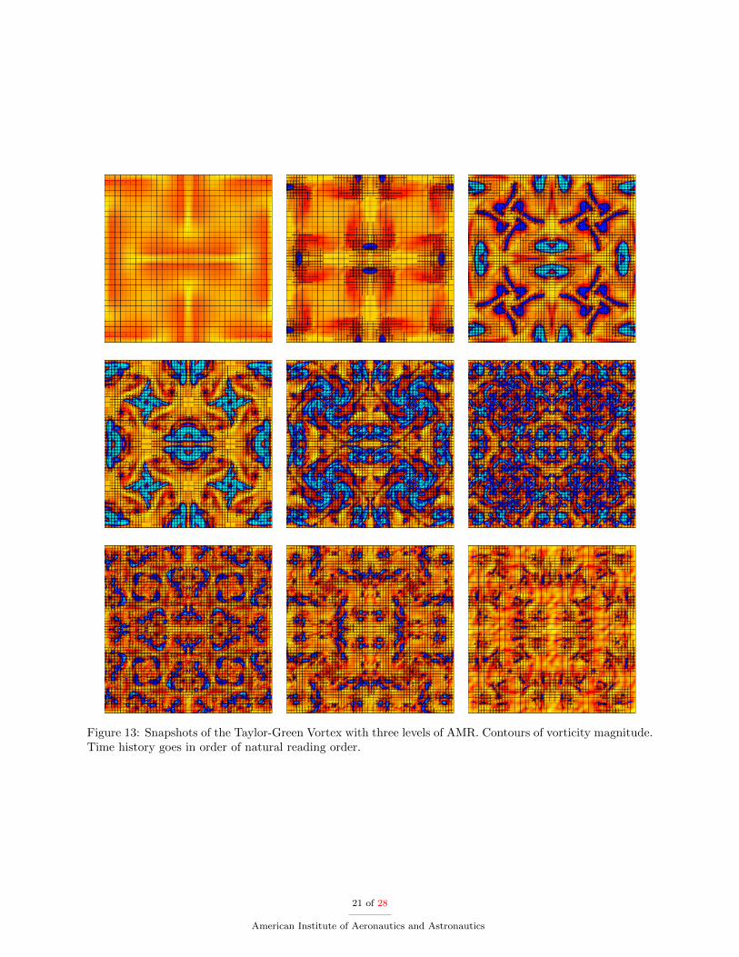
Figure 13: Snapshots of the Taylor-Green Vortex with three levels of AMR. Contours of vorticity magnitude.Time history goes in order of natural reading order.
21 of 28
American Institute of Aeronautics and Astronautics
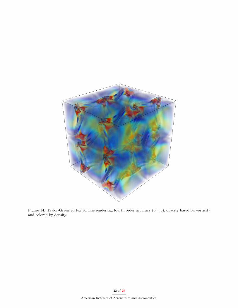
Figure 14: Taylor-Green vortex volume rendering, fourth order accuracy (p = 3), opacity based on vorticityand colored by density.
22 of 28
American Institute of Aeronautics and Astronautics
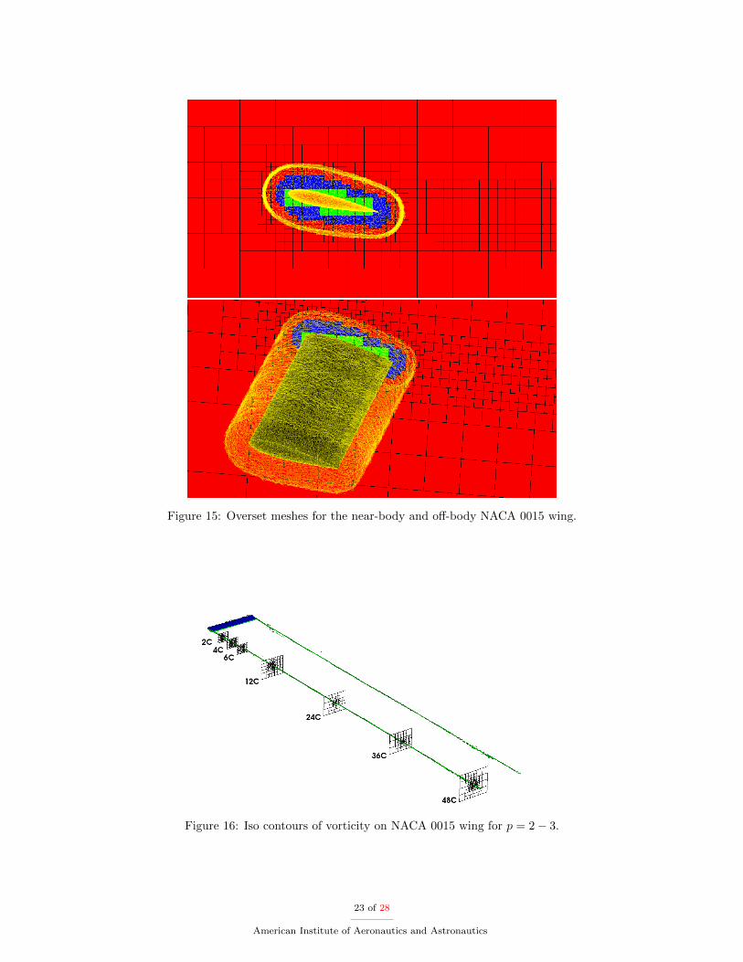
Figure 15: Overset meshes for the near-body and off-body NACA 0015 wing.
Figure 16: Iso contours of vorticity on NACA 0015 wing for p = 2− 3.
23 of 28
American Institute of Aeronautics and Astronautics
Iteration
Ne
ar
bo
dy
Re
sid
ua
l
0 20000 40000 60000 8000010
8
107
106
105
104
103
102
Iteration
CL
CD
0 20000 40000 60000 800000
0.2
0.4
0.6
0.8
1
0
0.2
0.4
0.6
0.8
1
Figure 17: Residual convergence (left) and coefficient of lift and drag convergence for NACA 0015 wing forp = 3− 5.
y
Vz
3.5 3 2.50.8
0.6
0.4
0.2
0
0.2
0.4
0.6
0.8
WAKE3Dp1
WAKE3Dp2/p3
WAKE3Dp3/p5
Experiment
(a) 1 chord downstream
y
Vz
3.5 3 2.50.8
0.6
0.4
0.2
0
0.2
0.4
0.6
0.8
WAKE3Dp1
WAKE3Dp2/p3
WAKE3Dp3/p5
Experiment
(b) 2 chords dowstream
y
Vz
3.5 3 2.50.8
0.6
0.4
0.2
0
0.2
0.4
0.6
0.8
WAKE3Dp1
WAKE3Dp2/p3
WAKE3Dp3/p5
Experiment
(c) 4 chords downstream
y
Vz
3.5 3 2.50.8
0.6
0.4
0.2
0
0.2
0.4
0.6
0.8
WAKE3Dp1
WAKE3Dp2/p3
WAKE3Dp3/p5
Experiment
(d) 6 chords downstream
Figure 18: Velocity wake profile downstream from wing for polynomial degrees p = 1, p = 2−3, and p = 3−5.
24 of 28
American Institute of Aeronautics and Astronautics
y
Vz
3.5 3 2.50.8
0.6
0.4
0.2
0
0.2
0.4
0.6
0.8WAKE3DHELIOSExperiment
(a) 2 chords downstream
y
Vz
3.5 3 2.50.8
0.6
0.4
0.2
0
0.2
0.4
0.6
0.8WAKE3DHELIOSExperiment
(b) 4 chords dowstream
y
Vz
3.5 3 2.50.8
0.6
0.4
0.2
0
0.2
0.4
0.6
0.8WAKE3DHELIOSExperiment
(c) 6 chords downstream
y
Vz
3.5 3 2.50.8
0.6
0.4
0.2
0
0.2
0.4
0.6
0.8WAKE3DHELIOS
(d) 12 chords downstream
Figure 19: Velocity wake profile downstream from wing for polynomial degrees p = 3− 5 and comparison toHELIOS.
25 of 28
American Institute of Aeronautics and Astronautics
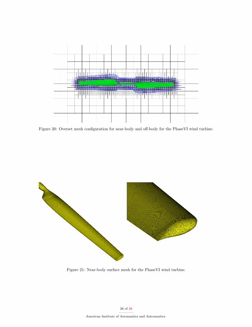
Figure 20: Overset mesh configuration for near-body and off-body for the PhaseVI wind turbine.
Figure 21: Near-body surface mesh for the PhaseVI wind turbine.
26 of 28
American Institute of Aeronautics and Astronautics
0 1000 2000 3000 4000 50000
1
2
3
4
5
6x 10
7
time steps
degre
es o
f fr
eedom
p=1
p=2
p=4
0 1000 2000 3000 4000 50000.2
0.4
0.6
0.8
1
1.2
1.4
1.6
1.8
2x 10
4
time steps
de
gre
es o
f fr
ee
do
m ∆
p=1
p=2
p=4
Figure 22: Degrees of freedom per time step (left) and derivative of quartic fit (right) for PhaseVI windturbine with freestream velocity 10 m/s.
Figure 23: PhaseVI wind turbine off-body mesh for p = 1 case (left) and p = 4 case (right) colored bypolynomial degree.
Figure 24: Contours of velocity magnitude for the PhaseVI wind turbine. Left image is p = 1 case and theright image is p = 4 case with mesh overlayed.
27 of 28
American Institute of Aeronautics and Astronautics
5 10 15 20 252
4
6
8
10
12
14
16
18
Wind Speed [m/s]
Pow
er
[kW
]
Experiment
Helios
Overflow
NSU3D
NSU3D+dg4est
5 10 15 20 25500
1000
1500
2000
2500
3000
3500
4000
4500
Wind Speed [m/s]
Thru
st [N
]
Experiment
Helios
Overflow
NSU3D
NSU3D+dg4est
Figure 25: NREL PhaseVI wind turbine power sweep (left) and thrust sweep (right).
28 of 28
American Institute of Aeronautics and Astronautics