INDOOR A* PATHFINDING THROUGH AN OCTREE REPRESENTATION … · 2.1 Pathfinding methods in octree structures . Herman (1986) present a combination of two pathfinding methods in an octree

INDOOR A* PATHFINDING THROUGH AN OCTREE REPRESENTATION

OF A POINT CLOUD

O.B.P.M. Rodenberg a, E. Verbree b *, S. Zlatanova c

a Delft University of Technology, Faculty of Architecture and the Built Environment, MSc Geomatics,

Julianalaan 134, 2628 BL, Delft, The Netherlands, [email protected] b Delft University of Technology, Faculty of Architecture and the Built Environment,

OTB - Research Institute for the Built Environment, GIS Technology,

Julianalaan 134, 2628 BL, Delft, The Netherlands, [email protected] c Delft University of Technology, Faculty of Architecture and the Built Environment,

Department of Urbanism, 3D Geoinformation,

Julianalaan 134, 2628 BL, Delft, The Netherlands, [email protected]

Commission IV

KEY WORDS: Indoor pathfinding, octree, network graph, connectivity, point cloud, collision avoidance

ABSTRACT:

There is a growing demand of 3D indoor pathfinding applications. Researched in the field of robotics during the last decades of the

20th century, these methods focussed on 2D navigation. Nowadays we would like to have the ability to help people navigate inside

buildings or send a drone inside a building when this is too dangerous for people. What these examples have in common is that an

object with a certain geometry needs to find an optimal collision free path between a start and goal point.

This paper presents a new workflow for pathfinding through an octree representation of a point cloud. We applied the following steps:

1) the point cloud is processed so it fits best in an octree; 2) during the octree generation the interior empty nodes are filtered and

further processed; 3) for each interior empty node the distance to the closest occupied node directly under it is computed; 4) a network

graph is computed for all empty nodes; 5) the A* pathfinding algorithm is conducted.

This workflow takes into account the connectivity for each node to all possible neighbours (face, edge and vertex and all sizes). Besides,

a collision avoidance system is pre-processed in two steps: first, the clearance of each empty node is computed, and then the maximal

crossing value between two empty neighbouring nodes is computed. The clearance is used to select interior empty nodes of appropriate

size and the maximal crossing value is used to filter the network graph. Finally, both these datasets are used in A* pathfinding.

1. INTRODUCTION

There is a growing demand of 3D indoor pathfinding applications

(Isikdag et al., 2013). Researched in the field of robotics during

the last decades of the 20th century, these methods focussed on

2D navigation. Besides the algorithms were developed for

relatively slow robots. Nowadays we would like to have the

ability to help people navigate inside buildings or send a drone

inside a building when this is too dangerous for people.

What these examples have in common is that an object with a

certain geometry needs to find an optimal collision free path

between a start and goal point. To manage this we need to know

the geometry of the object and a model of the environment. One

way of representing the latter one can be using a point cloud.

However, a point cloud of the environment alone does not give

enough information to find a route: for this, the empty (pointless)

space is needed. The empty space can be derived from the

occupied space by segmenting a point cloud.

A common method to structure and segment a point cloud is

through an octree data structure. An octree consists out of a

cubical volume which is recursively subdivided ‘into eight

congruent disjoint cubes (called octants) until blocks of a uniform

colour are obtained, or a predetermined level of decomposition is

reached’ (Samet, 1982). Here, ‘uniform colour’ indicates: the

block is completely empty or completely occupied. They are used

for the partitioning of space and result in a hierarchical tree

* Corresponding author

structure. This makes operations like neighbour finding and

indexing efficient (Vörös, 2000).

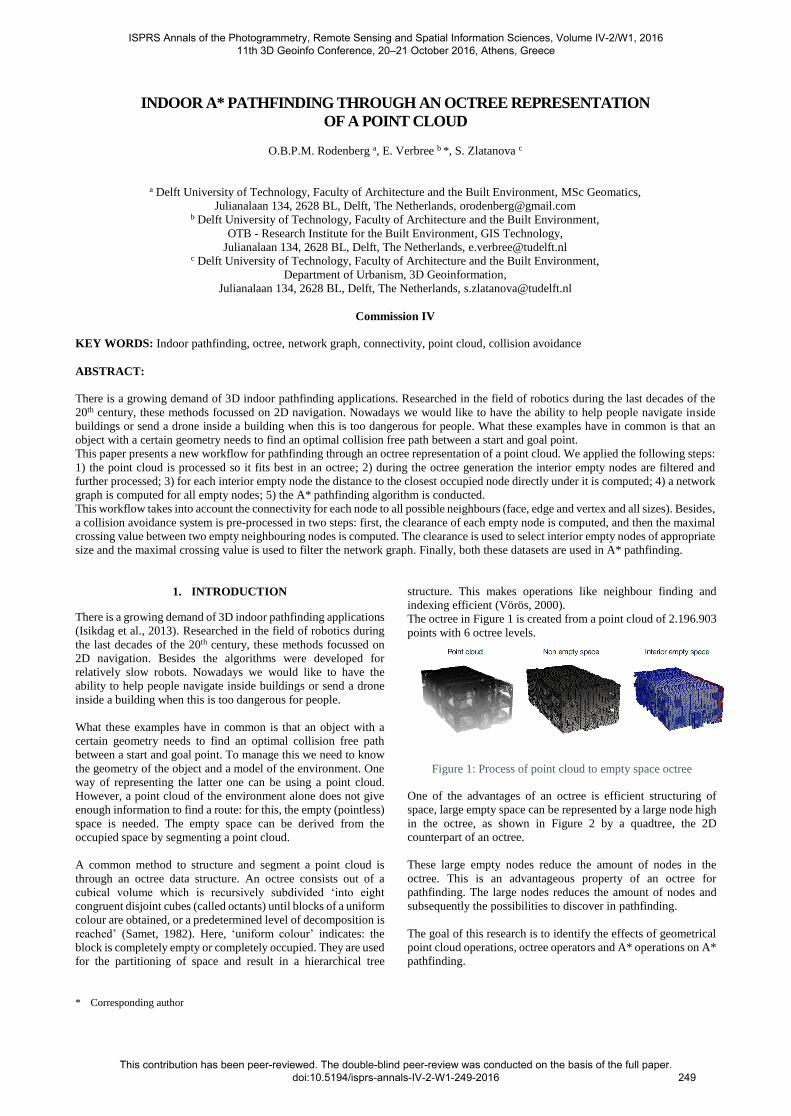
The octree in Figure 1 is created from a point cloud of 2.196.903

points with 6 octree levels.

Figure 1: Process of point cloud to empty space octree

One of the advantages of an octree is efficient structuring of

space, large empty space can be represented by a large node high

in the octree, as shown in Figure 2 by a quadtree, the 2D

counterpart of an octree.

These large empty nodes reduce the amount of nodes in the

octree. This is an advantageous property of an octree for

pathfinding. The large nodes reduces the amount of nodes and

subsequently the possibilities to discover in pathfinding.

The goal of this research is to identify the effects of geometrical

point cloud operations, octree operators and A* operations on A*

pathfinding.

ISPRS Annals of the Photogrammetry, Remote Sensing and Spatial Information Sciences, Volume IV-2/W1, 2016 11th 3D Geoinfo Conference, 20–21 October 2016, Athens, Greece

This contribution has been peer-reviewed. The double-blind peer-review was conducted on the basis of the full paper. doi:10.5194/isprs-annals-IV-2-W1-249-2016

249

mailto:[email protected]



The remainder of this paper is structured as follows: the second

section provides related work; section 3 presents the

methodology of the research; section 4 presents the tests and

results, and finally, section 5 discusses the validation tests and

concludes on the findings.

Figure 2: Subdivision of a quadtree, large empty space can be

constructed out of a single quadrant.

2. RELATED WORK

The related work of this research is threefold: pathfinding

methods in octree structures, neighbour finding methods in octree

data structures and finally collision avoidance methods.

2.1 Pathfinding methods in octree structures

Herman (1986) present a combination of two pathfinding

methods in an octree representation. It combines a hill climbing

(local optimisation) method in combination with an A*

algorithm. The A* algorithm is an extension of the Dijkstra

algorithm. The A* algorithm introduces a heuristic cost, which

approximates the cost from the marked node to the goal node

(Hart et al., 1968).

Hill climbing is able to quickly compute a path because it only

uses the distances to adjacent nodes to decide the next node.

However, this method has a tendency to stick in ‘U’ shaped

obstacles. When this happen an A* algorithm is used until the

obstacle is avoided. This method is fast, although it trends to

move away from the shortest route.

Vörös (2001) uses a hill climbing method in combination with a

distance map to compute a path in a quadtree and octree

representation. By using an octree representation instead of a

voxel approach the memory demand and pathfinding computing

time is reduced. The disadvantage of a distance map is the need

for a specific distance map for each distinct goal node.

Hwang and Ahuja (1992) use a potential field to navigate in an

octree. The potential field indicates a heuristic potential of each

node, in such a field there are local minima (nodes with a low

potential). First, a graph is computed between these local minima

and a global planner searches a path in the graph. Subsequently,

a local planner checks the path for collisions. If a collision is

found the path is deleted and the process restarts. A Dijkstra or

A* algorithm is used to navigate the graph.

Broersen et al. (2016) created a simple pathfinding algorithm

based on an A* algorithm. The route was computed through the

empty space in the octree. The pathfinding method considered

two nodes as neighbours if they share a common face.

Neighbours could be smaller, larger and of equal size. The

neighbours are computed on the fly and object avoidance was not

implemented.

Kambhampati and Davis (1985) propose a multi resolution

pathfinding method in a quadtree. To reduce the amount of leaf

nodes a pruned quadtree is created. In a pruned quadtree, grey

nodes containing empty (white) and occupied (black) are possible

neighbours.

2.2 Neighbour finding methods in octree data structures

All pathfinding algorithms rely on the exploration of adjacent

nodes. In an octree structure, two nodes can be each other’s

neighbour if they share a common: face, edge, or vertex. Figure

3 illustrates the types of connectivity’s. In total, there are 26

possible neighbours for each node. This section describes the

related work of neighbour finding.

Figure 3: Sharing a common face (6), edge (12), or vertex (8)

In the neighbour finding method of Gargantini (1982) motion is

possible in the face direction. Each octant in has a unique location

code. This location code describes the location of a node inside

the octree. A distinction is made between nodes sharing a

common parent and nodes having a different parent node.

Adjacent nodes are computed using a separate function for each

direction. The main drawback of this method is that the algorithm

does not know if a neighbour is part of the octree.

Samet (1989) proposes a method to compute face, edge and

vertex neighbours in all possible sizes (smaller, equal, and

larger). Neighbours are found by ascending the octree in search

of a common ancestor. The neighbouring node is found by

descending the tree with mirrored moves.

(Vörös, 2000) improved the method of (Samet, 1989) on three

areas. He used the work of Gargantini (1982) to implement the

difference between inner and outer neighbours. Using location

codes, the octree could be stored as linear area instead of a tree

structure. He uses a binary exclusive or operations on the

appropriate number of the location code and a directional

relevant bit mask to compute neighbours. Xu et al. (2015) checks

for face neighbours based on their geometrical location. Payeur

(2006) provides a method to search face, edge and vertex

neighbours in all possible sizes. For this, a lookup table is used.

Namdari et al. (2015) describes a method for neighbour finding

during the octree construction. The method is used to find all

face, edge and vertex neighbours in all sizes. The method is based

on a bread-first search octree generation. Meaning: from the root

node to the leaf nodes. The computational effort is minimized by

only searching equal and larger neighbours. To make sure also

smaller neighbours are stored a neighbouring connection is stored

in both directions. If node X has a neighbour node Y this

neighbour information should be stored in both node X and Y.

This last method ensures that smaller neighbours of a node are

found and stored in a later stage in the octree construction. The

actual approach in which neighbours are found is quite basic and



250

does not take advantage of the locational codes. It just checks if

two nodes share x, y and/or z coordinates.

2.3 Collision avoidance methods

Next, the related work on collision avoidance is presented: Jung

and Gupta (1996) use a distance map for collision detection. For

each node the distance to the closest object is calculated. In the

method, motion is not limited between centre points of nodes, as

instead motion is possible from any point in the octree. This

means two distance need to be stored.

Samet (1982) also uses a distance map to create a collision free

path in a quadtree. In contrast to Jung and Gupta (1996) motion

is only possible between the centre points of the nodes, so only

one distance value needs to be stored. An efficient way of finding

the closest neighbour is based on the theorem: not all equal sized

neighbouring nodes of a white node can be white since merging

between the nodes will take place and the white node would not

exist.

In a potential field approach, an artificial field is generated in

which both the target node and all obstacles direct a force on each

empty node in a field. The target node has an attractive force and

the obstacles have a repulsive force. These forces are strong at

the source and gradually decrease as the distance to the source

increase. The sum of these forces are the potential value of a

node, together all nodes form a potential field. The maximal

potential field is in the obstacles, a low potential field is thus

favourable in pathfinding applications (Hou and Zheng, 1994)

(Hwang and Ahuja, 1992). Wu and Hori (2006) use a potential

field to avoid obstacles. Hamada and Hori (1996) combine a

global path planner with al local path planner. Collision detection

is performed in the local path planner. Kambhampati and Davis

(1985) create a buffer around object to prevent collisions.

3. METHODOLOGY

3.1 Octree generation

An overview of the method is illustrated in Figure 4. The basic

idea of the method is to use an octree to segment a point cloud,

where the octree is used as a kind of catalyst for A* pathfinding.

The octree participates the pathfinding process. Before the octree

generation the point cloud is geometrical pre-processed. The

occupied (non-empty) and empty nodes are generated as

described in (Broersen et al., 2016). During the construction of

an empty node, it is checked if it is an interior or exterior empty

node. For each interior node, the distance to the closest occupied

node spatially directly beneath the node is computed. Next, the

possible neighbours and connectivity of the interior empty nodes

is computed and stored in a network graph. Using the possible

neighbours, a collision avoidance system is computed. The

network graph and interior empty space are used for A*

pathfinding.

3.2 Interior empty space

In this research, only interior point clouds are used for

pathfinding. These point clouds are scanned from the inside

therefore only the space between a point and the location of the

scanner can be classified as empty with certainty (Verbree,

2001). Therefore, it is key to identify the interior empty space for

cases like pathfinding and volume calculations.

The goal of identifying interior empty nodes is twofold. Firstly,

by identifying the interior empty nodes it is prevented for the

exterior empty nodes to be further processed and stored, which

reduces the amount of storage and computations. Secondly, only

the empty nodes, which are of interest, are used in pathfinding.

This avoids the path to exit the interior space via windows or

open areas.

Figure 4: Workflow of the method

An empty node is of the type ‘interior empty node’ if it has an

occupied node spatially straight above it. Figure 5 illustrates a

section of a building represented by a quadtree, all nodes that do

not have an occupied node (grey) above it are exterior empty

nodes (red), and the rest are interior empty nodes (green). To

check if a neighbour is interior, neighbours spatially above the

node need to be computed until a black node is reached (the node

is interior) or until there are no more neighbours (the node is

exterior). Only the interior empty nodes are further processed.

Figure 5: Occupied nodes (grey), interior empty nodes (green),

exterior empty nodes (red)



251

This method can also be used to compute the distance between

an interior empty node and the closest black node directly under

it. The distance can be used as a constraint in A* pathfinding. For

example, a maximum distance of 1 meter roughly represent the

volume in which a person can reach the closest black node

underneath him/her. By selecting a start and goal node maximal

1 meter above a black node the path will likely be bound to the

floor. Note that this method is very basic and there is no proof

that is will work in all circumstances.

3.3 Connectivity construction

To navigate through the empty space of an octree the connectivity

between the interior empty nodes must be known. Constructing

the connectivity of an interior empty node consist of two steps:

first all possible neighbours are computed, next the neighbours

that exist as interior empty nodes in the octree are selected.

3.3.1 Neighbour finding

The neighbour finding method is based on the work of Vörös

(2000), he proposes to find neighbours based on their common

ancestor. There are a number of differences between the method

of Vörös and the approach used in this research. Firstly, Vörös

computes neighbours that are smaller, equal, and larger. In this

research only neighbour that are equal and larger are needed, this

procedure will be explained in section 3.3.2. Secondly, in the

method of Vörös two nodes are neighbours if they share a

common face. In this research, two nodes can be neighbours if

they share a common: face, edge, and vertex. So the method of

Vörös is extended to compute the edge and vertex neighbours.

The equal and larger face neighbours are computed like the

method of Vörös. The method to compute larger neighbours work

the same for face, edge, and vertex neighbours.

The basic idea for finding edge neighbours is: the edge

neighbours of node c have a face connection with a face

neighbour of node c. The method is divided into four steps,

Figure 6 illustrates these steps. In the first step, the face

neighbours of node c are computed. In the second step the face

neighbour which are computed in the directions x and y are

selected. In the third step the neighbours in z and x are computed

of the face neighbours in direction x. In addition, the neighbours

in z of the face neighbours in direction y are computed. The

computed neighbours of the face neighbours form the complete

set of equal edge neighbours.

Figure 6: Edge neighbours - first step: face neighbours, second

step: selected face neighbours, third step: compute face

The method for computing equal vertex neighbours is similar to

that of edge neighbours. Vertex neighbours of node c have a face

connection with an edge neighbour of node c. The method is

divided into four steps, Figure 7 illustrates the steps. In the first

step, the edge neighbours are computed. Next the edge

neighbours which were computed in direction x are selected. Of

the selected node, the face neighbours in the direction z are

computed: these nodes are the vertex neighbours.

Figure 7: Face neighbours - First step: edge neighbours, second

step: selected edge neighbours, third step: compute face

3.3.2 Connectivity generation

In this step, the neighbours computed in the section 3.3.1 are used

to select neighbours that are interior empty nodes. All occupied

nodes are filtered out. The method of Namdari et al. (2015) is

used to compute neighbours during bread-first search octree

generation. In the method, only equal and larger neighbours are

computed. By storing the connection of a larger neighbour in

both connected nodes, also smaller neighbours are found in a

later stage of the octree generation. Like the method of Namdari

et al. (2015), the octree used in this research is computed in a top

down approach. For each white node that is computed, the equal

and larger neighbours are computed based on the method

described in in the previous part of this section. For each larger

neighbour the connection is stored in both directions if the larger

neighbour is an empty node. For example, if node x has a larger

neighbours y the connection in node x and node y is stored. This

step ensures that for the larger node y the smaller neighbours are

stored. For each connection, the cost is computed and stored in a

network graph.

3.4 Collision avoidance

The goal of collision avoidance is to compute a path for an object

in which a collision is not possible. A path is collision free if the

object does not intersect with any occupied node along the path.

For this, we need to know: can an object, with a certain size, fit

in an interior empty node, and can this object move between two

neighbouring empty nodes. Therefore this section consist of two

parts: the first part explains how to compute the distance from the

centre of an interior empty node to the closest border with an

occupied node. In addition, the second part explains how to

compute the distance between a crossing point and the closest

black node.

The method of Samet (1982) is used to compute the clearance for

each empty node. He describes a theorem that states: All

neighbours of a white node cannot all be white because merging

would take place and the node would not exist.

The closest boundary with an occupied node is computed with a

chessboard distance. Thus the closest occupied node must be, or

a descendant of, one of the equal neighbours (see Figure 8). Since

occupied nodes are always stored in the lowest level, an occupied

node can never be a larger neighbour. So the 26 equal neighbours

are needed to find the closest boundary with an occupied node.

Since these neighbours were computed and stored during the

connectivity generation these are already available. To acquire

the closest boundary the set of neighbours is compared with the

set of occupied nodes. For each occupied node intersecting with

the neighbours, the distance between the border of the occupied

node and the centre point of the empty node is computed. As it is

possible for multiple occupied nodes to intersect, it is the smallest

distance that defines the clearance. The clearance of all interior

empty nodes form a clearance map.



252

Figure 8: The closest border with a black node and the dark blue

node must lie in the light blue area

Figure 9 shows two diagrams, in the left, an object (blue circle)

is in the centre of an empty node where the clearance is sufficient.

Although the clearance is sufficient in the centre point of a node,

the object collides with an occupied node (red) when moving

between two empty nodes. For this reason it is key to check the

maximal crossing value for each connection between two empty

nodes. This crossing value can never be bigger than the minimal

clearance of the two connection empty nodes. Otherwise, an

object would be able to enter a node with a clearance smaller than

the object size and a collision would occur.

Figure 9: Collision avoidance: Centre point is collision free

(left), but movement collides (right)

The next step is to compute the maximal crossing value between

two neighbouring interior empty nodes. Figure 10 shows an

object on an intersection between two adjacent empty nodes. The

only place in the intersection where the distance to a black node

can be smaller than the clearance of one of the two empty nodes

is in the two red nodes. To find the closest occupied node the

nodes in the red areas are compared with the set of occupied

nodes. For each occupied node that intersects with the red area

the distance to the crossing is computed. In general, the minimal

distance is the crossing value. However, if the minimal distance

exceeds the clearance of one of the nodes the minimal clearance

defines the maximal crossing value. Also, if no occupied nodes

are found in the area the maximal crossing value is defined by the

minimal clearance. The crossing value is stored in a network

graph aside the cost between two empty nodes.

Figure 10: Collision avoidance: The area that must be checked

for occupied nodes

4. TEST AND RESULTS

4.1 Point cloud processing

The point cloud is geometrical pre-processed in the following

order: The point cloud is first rotated so it is aligned with the axis.

Next, the rotated point cloud is translated so the origin of the

point cloud has coordinate (0, 0, 0). Finally, the point cloud is

scaled so it fits best in an octree grid of 2n * 2n * 2n. Where n

refers to the octree depth. Figure 11 illustrates this process.

Figure 11: Pre-processing the point cloud

4.2 Filtering interior empty nodes

During the octree generation the interior and exterior empty

space are identified. All exterior empty space is no further

processed. Figure 12 illustrates the difference between the

interior and exterior empty space. In this example, 5699 exterior

empty space nodes are filtered out on 11348 interior empty

nodes.

Figure 12: Filtering of interior empty nodes

4.3 Octree generation

Figure 1 illustrates the total process of identifying the interior

empty nodes of a point cloud. The octree in Figure 1 is created

from a point cloud of 2.196.903 points with 6 octree levels.

The computer used in the test has an Intel(R) Core(TM) i5-4590

CPU @3.30GHz processor, 8.00 GB RAM running Windows 10

Pro 64 bits.



253

All scripts are written in the programming language ’python’. For

the database management, postgreSQL was used. To connect

Python to postgreSQL, the package psycopg2 is used. The

package LibLas is used to work with .las files (point clouds) in

python. For visualizations, the open source software Paraview is

used.

4.4 Connectivity generation

Figure 13 illustrates the process of generating the connectivity of

a current interior empty node. First all possible neighbours are

computed. Finally, all nodes in the possible neighbours

intersecting with an occupied node are excluded. Besides, a

neighbour is always stored as big as possible; this excludes

neighbours that are children nodes of bigger neighbours.

Figure 13: Connectivity generation

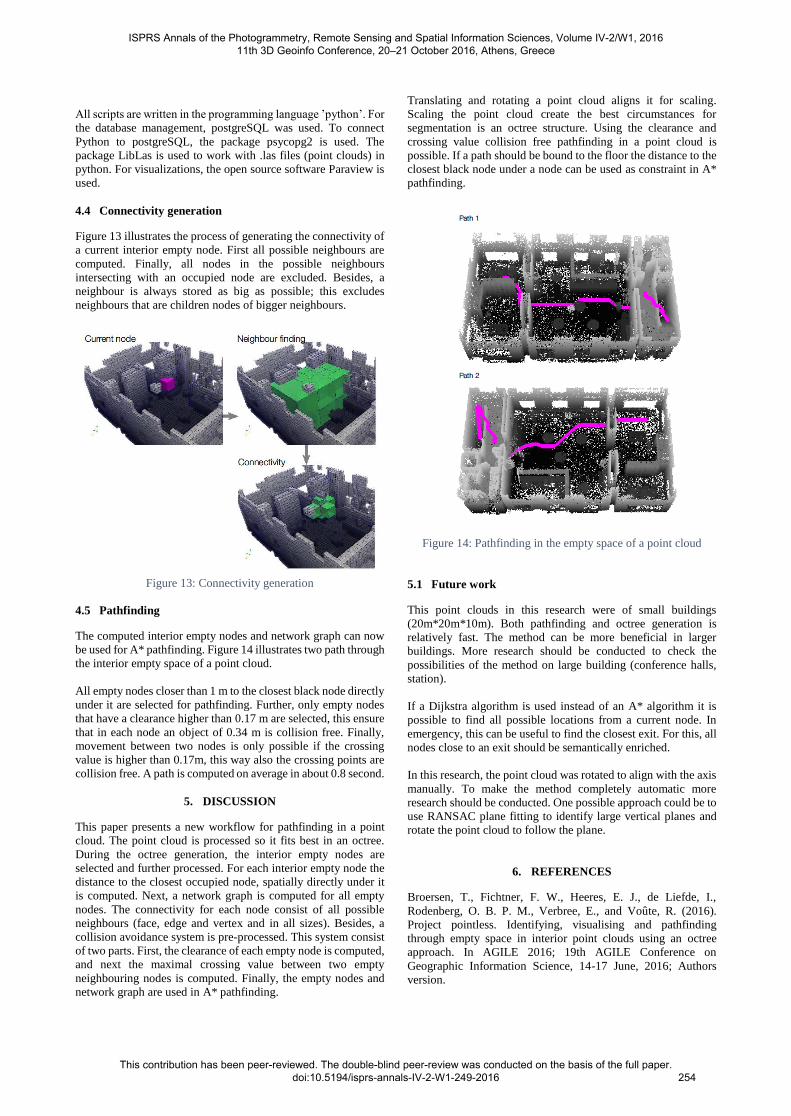
4.5 Pathfinding

The computed interior empty nodes and network graph can now

be used for A* pathfinding. Figure 14 illustrates two path through

the interior empty space of a point cloud.

All empty nodes closer than 1 m to the closest black node directly

under it are selected for pathfinding. Further, only empty nodes

that have a clearance higher than 0.17 m are selected, this ensure

that in each node an object of 0.34 m is collision free. Finally,

movement between two nodes is only possible if the crossing

value is higher than 0.17m, this way also the crossing points are

collision free. A path is computed on average in about 0.8 second.

5. DISCUSSION

This paper presents a new workflow for pathfinding in a point

cloud. The point cloud is processed so it fits best in an octree.

During the octree generation, the interior empty nodes are

selected and further processed. For each interior empty node the

distance to the closest occupied node, spatially directly under it

is computed. Next, a network graph is computed for all empty

nodes. The connectivity for each node consist of all possible

neighbours (face, edge and vertex and in all sizes). Besides, a

collision avoidance system is pre-processed. This system consist

of two parts. First, the clearance of each empty node is computed,

and next the maximal crossing value between two empty

neighbouring nodes is computed. Finally, the empty nodes and

network graph are used in A* pathfinding.

Translating and rotating a point cloud aligns it for scaling.

Scaling the point cloud create the best circumstances for

segmentation is an octree structure. Using the clearance and

crossing value collision free pathfinding in a point cloud is

possible. If a path should be bound to the floor the distance to the

closest black node under a node can be used as constraint in A*

pathfinding.

Figure 14: Pathfinding in the empty space of a point cloud

5.1 Future work

This point clouds in this research were of small buildings

(20m*20m*10m). Both pathfinding and octree generation is

relatively fast. The method can be more beneficial in larger

buildings. More research should be conducted to check the

possibilities of the method on large building (conference halls,

station).

If a Dijkstra algorithm is used instead of an A* algorithm it is

possible to find all possible locations from a current node. In

emergency, this can be useful to find the closest exit. For this, all

nodes close to an exit should be semantically enriched.

In this research, the point cloud was rotated to align with the axis

manually. To make the method completely automatic more

research should be conducted. One possible approach could be to

use RANSAC plane fitting to identify large vertical planes and

rotate the point cloud to follow the plane.

6. REFERENCES

Broersen, T., Fichtner, F. W., Heeres, E. J., de Liefde, I.,

Rodenberg, O. B. P. M., Verbree, E., and Voûte, R. (2016).

Project pointless. Identifying, visualising and pathfinding

through empty space in interior point clouds using an octree

approach. In AGILE 2016; 19th AGILE Conference on

Geographic Information Science, 14-17 June, 2016; Authors

version.



254

Gargantini, I. (1982). Linear octrees for fast processing of three-

dimensional objects. Computer graphics and Image processing,

20(4):365–374. Guang-lei, Z. and He-Ming, J. (2012). Global

path planning of AUV based on improved ant colony

optimization algorithm. In Automation and Logistics (ICAL),

2012 IEEE International Conference on, pages 606–610. IEEE.

Hamada, K. and Hori, Y. (1996). Octree-based approach to real-

time collision-free path planning for robot manipulator. In

Advanced Motion Control, 1996. AMC’96-MIE. Proceedings

1996 4th International Workshop, volume 2, pages 705–710.

IEEE.

Hart, P. E., Nilsson, N. J., and Raphael, B. (1968). A formal basis

for the heuristic determination of minimum cost paths. Systems

Science and Cybernetics, IEEE Transactions on, 4(2):100–107.

Herman, M. (1986). Fast, three-dimensional, collision-free

motion planning. In Robotics and Automation. Proceedings.

1986 IEEE International Conference on, volume 3, pages 1056–

1063. IEEE.

Hou, E. S. and Zheng, D. (1994). Mobile robot path planning

based on hierarchical hexagonal decomposition and artificial

potential fields. Journal of Robotic Systems, 11(7):605–614.

Hwang, Y. K. and Ahuja, N. (1992). A potential field approach

to path planning. Robotics and Automation, IEEE Transactions

on, 8(1):23–32.

Isikdag, U., Zlatanova, S., and Underwood, J. (2013). A BIM-

Oriented Model for supporting indoor navigation requirements.

Computers, Environment and Urban Systems, 41:112–123.

Jung, D. and Gupta, K. K. (1996). Octree-based hierarchical

distance maps for collision detection. In Robotics and

Automation, 1996. Proceedings., 1996 IEEE International

Conference on, volume 1, pages 454–459. IEEE.

Kambhampati, S. and Davis, L. S. (1985). Multiresolution path

planning for mobile robots. Technical report, DTIC Document.

Kim, J. and Lee, S. (2009). Fast neighbor cells finding method

for multiple octree representation. In 2009 IEEE International

Symposium on Computational Intelligence in Robotics and

Automation - (CIRA).

Namdari, M. H., Hejazi, S. R., and Palhang, M. (2015). Mcpn,

octree neighbor finding during tree model construction using

parental neighboring rule. 3D Research, 6(3):1–15.

Payeur, P. (2006). A computational technique for free space

localization in 3- d multiresolution probabilistic environment

models. Instrumentation and Measurement, IEEE Transactions

on, 55(5):1734–1746.

Samet, H. (1982). Distance transform for images represented by

quadtrees. Pattern Analysis and Machine Intelligence, IEEE

Transactions on, (3):298–303.

Samet, H. (1989). Neighbor finding in images represented by

octrees. Computer Vision, Graphics, and Image Processing,

46(3):367–386. van Oosterom, P. and Vijlbrief, T. (1996). The

spatial location code. In Proceedings of the 7th international

symposium on spatial data handling, Delft, The Netherlands.

Verbree, E. (2003). The STIN Method: 3D-Surface

reconstruction by observation lines and Delaunay TENs, ISPRS

Archives – Volume XXXIV-3/W13, 2003

Vörös, J. (2000). A strategy for repetitive neighbor finding in

octree representations. Image and Vision Computing,

18(14):1085–1091.

Vörös, J. (2001). Low-cost implementation of distance maps for

path planning using matrix quadtrees and octrees. Robotics and

Computer-Integrated Manufacturing, 17(6):447–459.

Wu, L. and Hori, Y. (2006). Real-time collision-free path

planning for robot manipulator based on octree model. In

Advanced Motion Control, 2006. 9th IEEE International

Workshop on, pages 284–288. IEEE.

Xu, S., Honegger, D., Pollefeys, M., and Heng, L. (2015). Real-

time 3d navigation for autonomous vision-guided mavs. IROS.



255

Documents

INDOOR A* PATHFINDING THROUGH AN OCTREE REPRESENTATION … · 2.1 Pathfinding methods in octree structures . Herman (1986) present a combination of two pathfinding methods in an octree