fer-

e

, is well

e rep-

rovide

jects

which

unit to

ation

r the

create

e local

Automatic Generation of Octree-based Three-DimensionalDiscretizations for Partition of Unity Methods

Ottmar Klaas and Mark S. ShephardScientific Computation Research Center

Rensselear Polytechnic Institute110 8th St., Troy, NY 12180

USAemail: oklaas@scorec.rpi.edu

Abstract: The Partition of Unity Method (PUM) can be used to numerically solve a set of dif

ential equations on a domainΩ. The method is based on the definition of overlapping patches

comprising a cover of the domainΩ. For an efficient implementation it is important that th

interaction between the patches themselves, and between the patches and the boundary

understood and easily accessible during runtime of the program. We will show that an octre

resentation of the domain with a tetrahedral mesh at the boundary is an efficient means to p

the needed information. It subdivides an arbitrary domain into simply shaped topological ob

(cubes, tetrahedrons) giving a non-overlapping discrete representation of the domain on

efficient numerical integration schemes can be employed. The octants serve as the basic

construct the overlapping partitions. The structure of the octree allows the efficient determin

of patch interactions.

1. Introduction

Partition of Unity methods are capable of constructing conforming solution spaces used fo

numerical solution of a set of differential equations on a domainΩ. They allow the inclusion of

local properties of the solution into the constructed solution space. The basic idea is to

overlapping patches comprising a cover of the domainΩ with partitions of unity

subordinate to the cover . On each patch local function spaces are set up reflecting th

Ωi

Ωi

Ωi Ωi ϕi

Ωi Vi

1

d on

ent

t Free

uare

. No

lapping

opular.

ter and

om-

task of

rather

creti-

ertain

oving

on inte-

ndary

ficult.

me the

sed for

uited

hich

shape

solution behavior. The global solution space is then given by . Methods base

that principle were developed by Babuska et al. [1],[2] (Partition of Unity Finite Elem

Method), and Duarte and Oden [7],[8] (hp - clouds). Similar methods referred to as Elemen

Galerkin Methods were developed by Belytschko et. al. [5], [11] or the Moving Least Sq

Reproducing Kernel Methods by Liu et al. [10].

One way to create the partition of unity is to start from an arbitrarily distributed set of nodes

fixed connections between the nodes are required. The nodes are the centers of the over

patches , which can have almost any shape with cubes and spheres among the most p

The partition of unity is then created based on the moving least square scheme (see Lancas

Salkauskas [9]). Advocators of this method praise the simplicity with which geometrically c

plex situations, like cracks, free surfaces etc., can be treated. The sometimes cumbersome

meshing and remeshing of a valid finite element mesh can be avoided. However, due to the

unstructured distribution of nodes over the domain other algorithmic issues arise. First, a dis

zation without structure does not allow determination of the patches that contribute to a c

integration point without performing a search. Second, the partition of unity based on the m

least square method creates shape functions that are expensive to integrate with the comm

gration rules, like Gauss quadrature formulas. Last, but not least, the treatment of the bou

conditions, and the interaction with the geometric boundary in general, becomes very dif

Recently, Duarte, Babuska and Oden [7] proposed to use a Finite Element mesh to overco

problems associated with an arbitrarily scattered set of nodes. The finite element mesh is u

the purpose of creating the partition of unity. The main difference to a mesh that would be s

for a finite element analysis is the lack of h-adaptation for singularities or steep gradients, w

simplifies the process of mesh generation slightly. Instead, the singularities are captured by

V V ϕiVii∑=

Ωi

2

od of

rahe-

ach a

search-

finite

ution.

The

as to be

tation

ce the

of the

n than

ide a

parti-

To be

eing

l con-

uct the

they

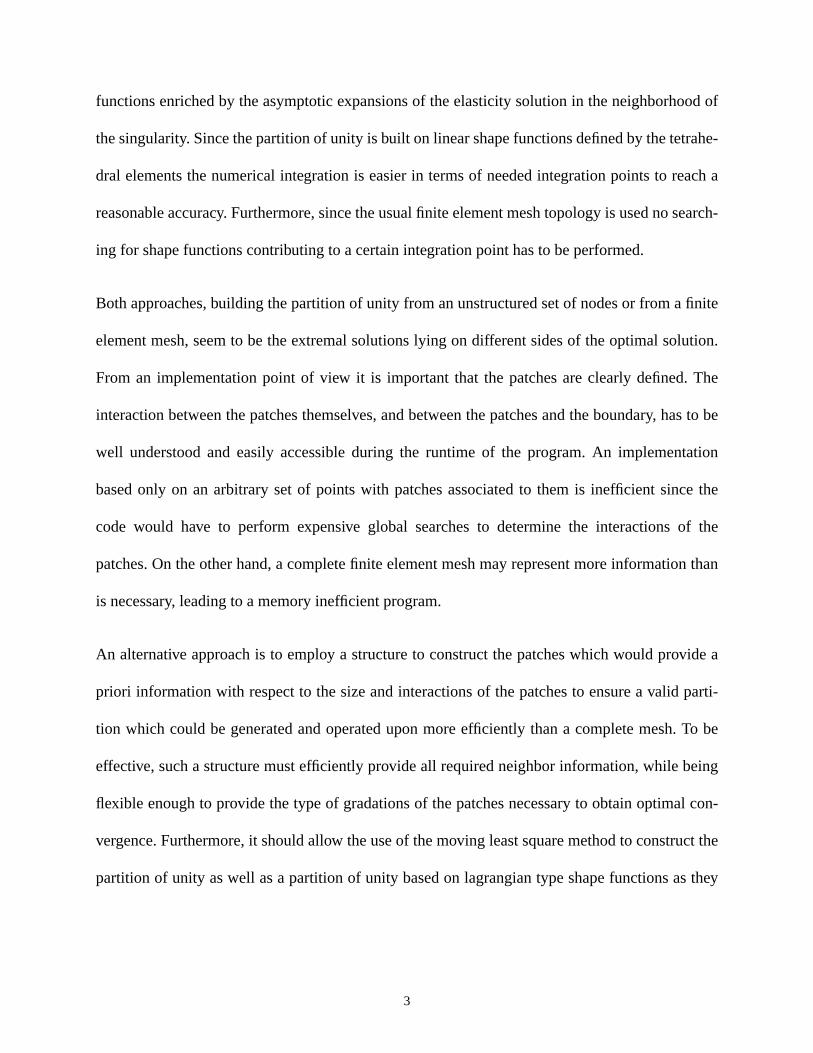
functions enriched by the asymptotic expansions of the elasticity solution in the neighborho

the singularity. Since the partition of unity is built on linear shape functions defined by the tet

dral elements the numerical integration is easier in terms of needed integration points to re

reasonable accuracy. Furthermore, since the usual finite element mesh topology is used no

ing for shape functions contributing to a certain integration point has to be performed.

Both approaches, building the partition of unity from an unstructured set of nodes or from a

element mesh, seem to be the extremal solutions lying on different sides of the optimal sol

From an implementation point of view it is important that the patches are clearly defined.

interaction between the patches themselves, and between the patches and the boundary, h

well understood and easily accessible during the runtime of the program. An implemen

based only on an arbitrary set of points with patches associated to them is inefficient sin

code would have to perform expensive global searches to determine the interactions

patches. On the other hand, a complete finite element mesh may represent more informatio

is necessary, leading to a memory inefficient program.

An alternative approach is to employ a structure to construct the patches which would prov

priori information with respect to the size and interactions of the patches to ensure a valid

tion which could be generated and operated upon more efficiently than a complete mesh.

effective, such a structure must efficiently provide all required neighbor information, while b

flexible enough to provide the type of gradations of the patches necessary to obtain optima

vergence. Furthermore, it should allow the use of the moving least square method to constr

partition of unity as well as a partition of unity based on lagrangian type shape functions as

3

e to be

esh at

haped

of the

rve as

tions.

s can

. Last

ite ele-

needs

e basic

how

ction 5

three

orting

enera-

ed by

n in

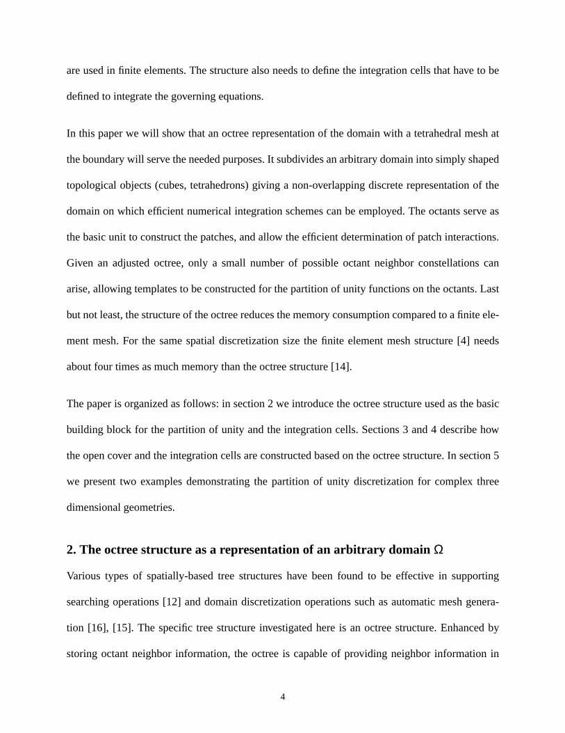
are used in finite elements. The structure also needs to define the integration cells that hav

defined to integrate the governing equations.

In this paper we will show that an octree representation of the domain with a tetrahedral m

the boundary will serve the needed purposes. It subdivides an arbitrary domain into simply s

topological objects (cubes, tetrahedrons) giving a non-overlapping discrete representation

domain on which efficient numerical integration schemes can be employed. The octants se

the basic unit to construct the patches, and allow the efficient determination of patch interac

Given an adjusted octree, only a small number of possible octant neighbor constellation

arise, allowing templates to be constructed for the partition of unity functions on the octants

but not least, the structure of the octree reduces the memory consumption compared to a fin

ment mesh. For the same spatial discretization size the finite element mesh structure [4]

about four times as much memory than the octree structure [14].

The paper is organized as follows: in section 2 we introduce the octree structure used as th

building block for the partition of unity and the integration cells. Sections 3 and 4 describe

the open cover and the integration cells are constructed based on the octree structure. In se

we present two examples demonstrating the partition of unity discretization for complex

dimensional geometries.

2. The octree structure as a representation of an arbitrary domainΩ

Various types of spatially-based tree structures have been found to be effective in supp

searching operations [12] and domain discretization operations such as automatic mesh g

tion [16], [15]. The specific tree structure investigated here is an octree structure. Enhanc

storing octant neighbor information, the octree is capable of providing neighbor informatio

4

iffer-

octant

ot by

levels

rred to

g data

rooted

is

g the

f an

inal

ion of

t ,

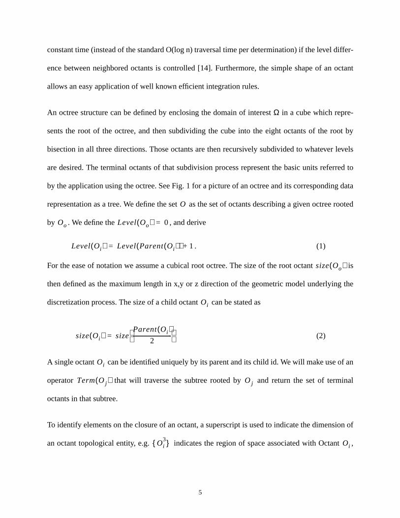
constant time (instead of the standard O(log n) traversal time per determination) if the level d

ence between neighbored octants is controlled [14]. Furthermore, the simple shape of an

allows an easy application of well known efficient integration rules.

An octree structure can be defined by enclosing the domain of interestΩ in a cube which repre-

sents the root of the octree, and then subdividing the cube into the eight octants of the ro

bisection in all three directions. Those octants are then recursively subdivided to whatever

are desired. The terminal octants of that subdivision process represent the basic units refe

by the application using the octree. See Fig. 1 for a picture of an octree and its correspondin

representation as a tree. We define the set as the set of octants describing a given octree

by . We define the , and derive

. (1)

For the ease of notation we assume a cubical root octree. The size of the root octant

then defined as the maximum length in x,y or z direction of the geometric model underlyin

discretization process. The size of a child octant can be stated as

(2)

A single octant can be identified uniquely by its parent and its child id. We will make use o

operator that will traverse the subtree rooted by and return the set of term

octants in that subtree.

To identify elements on the closure of an octant, a superscript is used to indicate the dimens

an octant topological entity, e.g. indicates the region of space associated with Octan

O

Oo Level Oo( ) 0=

Level Oi( ) Level Parent Oi( )( ) 1+=

size Oo( )

Oi

size Oi( ) sizeParent Oi( )

2-----------------------------

=

Oi

Term Oj( ) Oj

Oi3 Oi

5

e the

minal

interior

mbed-

ide

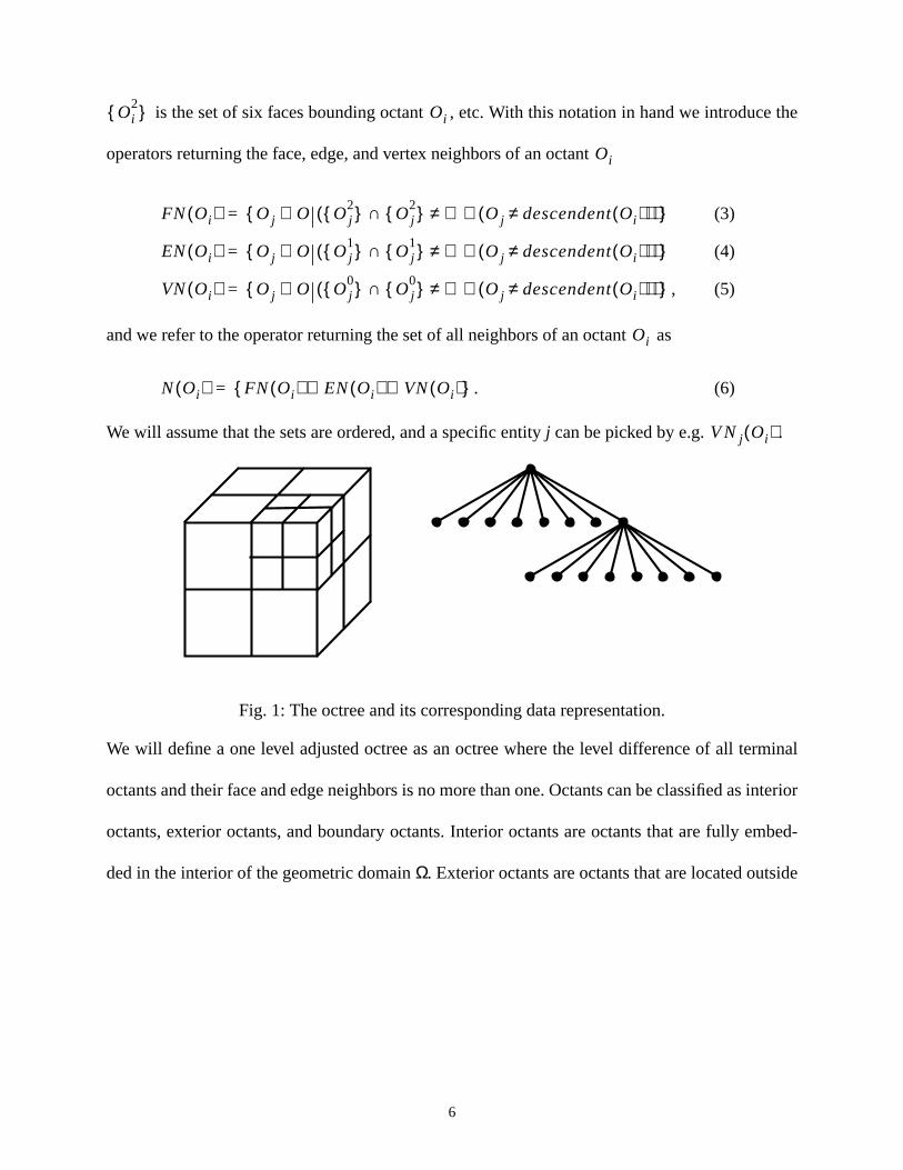
is the set of six faces bounding octant , etc. With this notation in hand we introduc

operators returning the face, edge, and vertex neighbors of an octant

(3)

(4)

, (5)

and we refer to the operator returning the set of all neighbors of an octant as

. (6)

We will assume that the sets are ordered, and a specific entityj can be picked by e.g. .

Fig. 1: The octree and its corresponding data representation.

We will define a one level adjusted octree as an octree where the level difference of all ter

octants and their face and edge neighbors is no more than one. Octants can be classified as

octants, exterior octants, and boundary octants. Interior octants are octants that are fully e

ded in the interior of the geometric domainΩ. Exterior octants are octants that are located outs

Oi2 Oi

Oi

FN Oi( ) Oj O∈ Oj2 Oj

2 ∩ ∅≠ Oj descendent Oi( )≠( )∧( ) =

EN Oi( ) Oj O∈ Oj1 Oj

1 ∩ ∅≠ Oj descendent Oi( )≠( )∧( ) =

VN Oi( ) Oj O∈ Oj0 Oj

0 ∩ ∅≠ Oj descendent Oi( )≠( )∧( ) =

Oi

N Oi( ) FN Oi( ) EN Oi( )∪ VN Oi( )∪ =

V Nj Oi( )

6

y the

the

in the

r and

intro-

dis-

t are

orm a

. The

n cover

size for

usu-

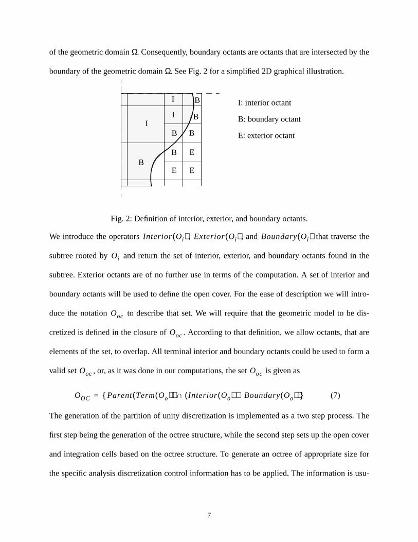
of the geometric domainΩ. Consequently, boundary octants are octants that are intersected b

boundary of the geometric domainΩ. See Fig. 2 for a simplified 2D graphical illustration.

Fig. 2: Definition of interior, exterior, and boundary octants.

We introduce the operators , , and that traverse

subtree rooted by and return the set of interior, exterior, and boundary octants found

subtree. Exterior octants are of no further use in terms of the computation. A set of interio

boundary octants will be used to define the open cover. For the ease of description we will

duce the notation to describe that set. We will require that the geometric model to be

cretized is defined in the closure of . According to that definition, we allow octants, tha

elements of the set, to overlap. All terminal interior and boundary octants could be used to f

valid set , or, as it was done in our computations, the set is given as

(7)

The generation of the partition of unity discretization is implemented as a two step process

first step being the generation of the octree structure, while the second step sets up the ope

and integration cells based on the octree structure. To generate an octree of appropriate

the specific analysis discretization control information has to be applied. The information is

E

EE

B

B

B

B

B

I

I

I

B

I: interior octant

B: boundary octant

E: exterior octant

Interior Oi( ) Exterior Oi( ) Boundary Oi( )

Oi

Ooc

Ooc

Ooc Ooc

OOC Parent Term Oo( )( ) Interior Oo( ) Boundary Oo( )∪( )∩ =

7

ures

cribing

trols

l ele-

been

losure

size

rior,

sh is

the con-

e used

ed not

octant

ts can

ach

of the

bound-

plica-

e fol-

f the

ointers

[14].

ally applied to the topological entities of the geometric model in the form of absolute meas

(e.g. maximum size of terminal octants) or relative measures (e.g. percentage error in des

curved boundaries). In terms of the to-be-constructed partition of unity, the information con

the size of the integration cells, which will be the terminal interior octants and tetrahedra

ments generated in the boundary octants. After the discretization control information has

applied a root octant is determined such that the geometric model is contained within the c

of that octant. Recursively subdividing that octant and its children to the level dictated by the

control information, while maintaining the type of the newly created octants (interior, exte

boundary), yields the octree fulfilling the control information. As a last step a tetrahedral me

generated in the boundary octants. References [16] and [6] discuss issues associated with

struction of the octrees as used in automatic mesh generation. The generation of the octre

here follows the same basic steps with the exception that the octants interior to the model ne

be decomposed into finite elements. Given an octree structure created based on any form is

size control, the algorithm for defining the one level difference between face and edge octan

be performed in time where is the number of original octants using the appro

given in reference [16]. The process of creating the tetrahedral elements to fill the portion

boundary octants interior to the domain uses exactly the same procedures used to mesh the

ary octants in the parallel mesh generator described given in reference [6].

The performance of h-refinement of interior octants is supported by the straightforward ap

tion of the recursive refinement procedure used to construct the original octree. This must b

lowed by an updating of the one-level difference criteria. Since the tree at that start o

refinement step already satisfies the one-level difference requirement, the face neighbor p

can be used to examine the neighbors to see if they need refinement in time [13],

O n nlog( ) n

O 1( )

8

the

tant is

ilar to

cells,

unity

g

t be

that

ds on

tches

vious

utations

iable

order

ving

ollect-

orting

are not

n of

Regaining the one-level difference can take from time if propagation is limited, and in

worst case is to if each and every octant needs to be refined [13]. When a boundary oc

refined the new boundary octants can be meshed using local remeshing procedures sim

those given in reference [3].

The sections, which follow describing the construction of the open cover and the integration

will assume that an octree, constructed as described, is available on which the partition of

discretization can be built.

3. Constructing an open cover ofΩ based on the octree structure

Overlapping patches comprise the open cover ofΩ. The patches serve as the buildin

blocks to form the partition of unity. For the partition of unity to be valid the patches can no

completely arbitrary. They have to fulfill certain requirements. First, it has to be guaranteed

each point in the domain of interest is covered by at least patches, where depen

the degree of the partition of unity. Second, the simplex formed by the center of the pa

must not degenerate. We refer to the Appendix for a detailed discussion of this issue. It is ob

that a method based on an arbitrary set of scattered nodes has to perform expensive comp

for each integration point to guarantee the validity of the discretization and ultimately the rel

solution based on the given set of nodes. Duarte and Oden [8] describe an algorithm of

O(NlogN) that checks the requirements for the partition of unity discretization based on mo

least square methods of order 0 and 1. The 2d-algorithm searches for the patches by c

ing a list of patches whose center falls into a bounding square around the point of interest, s

the list with respect to distance, and checking whether the center of at least three patches

aligned. The geometrical check for an alignment is not sufficient for higher order partitio

O 1( )

O n( )

Ωi Ωi

Nmin Nmin

Nmin

Nmin

9

ve to

a par-

s has

f order

an be

hat the

prob-

while

ment

ration.

ate than

nity

espite

les to

ts local

lution

ng as

d for a

ithmic

nteed a

unity, e.g. like they appear in the element free galerkin method. More complex algorithms ha

be employed. The Appendix describes in detail the requirements that have to be fulfilled for

tition of unity to be valid. As a last step the interaction between arbitrarily distributed patche

to be determined. This is again a searching problem where the best known algorithms are o

O(NlogN).

From the arguments made it becomes clear that the efficiency of partition of unity methods c

enhanced if the open cover is based on a suitable underlying structure. Suitable means t

chosen structure should support the method solving or at least reducing the implementation

lems associated with the flexibility of an arbitrary scattered set of patches of the open cover,

not restricting the features of the methods gained from exactly that flexibility. One main argu

for partition of unity methods is they do not necessarily need a mesh and avoid mesh gene

This argument translates into the demand for a structure that is easier and cheaper to gener

a classical Finite Element Mesh. Another important argument is the ability of partition of u

methods to support h-refinement by “throwing in” new patches wherever they are needed. D

the fact that the new patches can not be completely arbitrary, but have to follow certain ru

guarantee the validity of the open cover, the goal should be to create a structure that suppor

h-refinement. A third feature of meshless methods, the ability to easily adapt the local so

spaces to features of the actual solution, is not affected by the underlying structure as lo

those features (e.g. singularities) can be spatially resolved, which brings us back to the nee

support of local h-refinement.

An open cover based on an octree can provide the structure needed to simplify the algor

problems discussed above. The validity of the open cover based on an octree can be guara

10

or a

h, and

finite

ement

sump-

cture

ordi-

size of

he dis-

simple

ed by

e intro-

e

priori, i.e. no validity checks are necessary during runtime. We refer to the Appendix f

detailed discussion. The generation of an octree is more efficient than a finite element mes

h-refinement is easily possible since a valid adjusted octree has to follow far less rules than a

element mesh. Furthermore, the octree has very good localization capabilities allowing refin

of the discretization in areas of singularities if necessary. Last but not least, the memory con

tion is about four times smaller compared to a finite element structure [4] since the high stru

of the octree allows it to calculate needed information fast rather than storing it, e.g. the co

nates of the corners of an octant can be computed from the coordinate of the center and the

the octant.

For methods constructing the partition of unity based on the moving least square scheme t

cretization represented by an octree cannot directly be an open cover ofΩ since the spaces

represented by the cells of an octree are closed and do not overlap. However, there are two

possibilities to create a valid open cover based on the given octree structure distinguish

whether the patches are centered around the center or around the corners of the octants. W

duce the following two definitions describing the creation of the open cover.

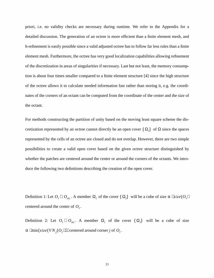
Definition 1: Let . A member of the cover will be a cube of size

centered around the center of .

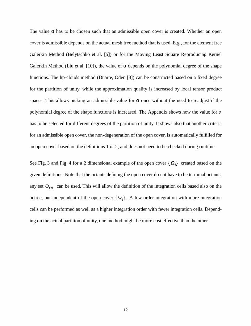
Definition 2: Let . A member of the cover will be a cube of siz

centered around cornerj of .

Ωi

Oi Ooc∈ Ωi Ωi α size Oi( )⋅

Oi

Oi Ooc∈ Ωi Ωi

α min size V Nj Oi( )( )( )⋅ Oi

11

open

ent free

rnel

pe

degree

uct

e

for

riteria

d for

time.

on the

tants,

n the

tion

pend-

The valueα has to be chosen such that an admissible open cover is created. Whether an

cover is admissible depends on the actual mesh free method that is used. E.g., for the elem

Galerkin Method (Belytschko et al. [5]) or for the Moving Least Square Reproducing Ke

Galerkin Method (Liu et al. [10]), the value ofα depends on the polynomial degree of the sha

functions. The hp-clouds method (Duarte, Oden [8]) can be constructed based on a fixed

for the partition of unity, while the approximation quality is increased by local tensor prod

spaces. This allows picking an admissible value forα once without the need to readjust if th

polynomial degree of the shape functions is increased. The Appendix shows how the valueα

has to be selected for different degrees of the partition of unity. It shows also that another c

for an admissible open cover, the non-degeneration of the open cover, is automatically fulfille

an open cover based on the definitions 1 or 2, and does not need to be checked during run

See Fig. 3 and Fig. 4 for a 2 dimensional example of the open cover created based

given definitions. Note that the octants defining the open cover do not have to be terminal oc

any set can be used. This will allow the definition of the integration cells based also o

octree, but independent of the open cover . A low order integration with more integra

cells can be performed as well as a higher integration order with fewer integration cells. De

ing on the actual partition of unity, one method might be more cost effective than the other.

Ωi

OOC

Ωi

12

ts.(see

ersectseded

Fig. 3: The definition of the open cover based on Definition 1.

Fig. 4: The definition of the open cover based on Definition 2.

Remark:

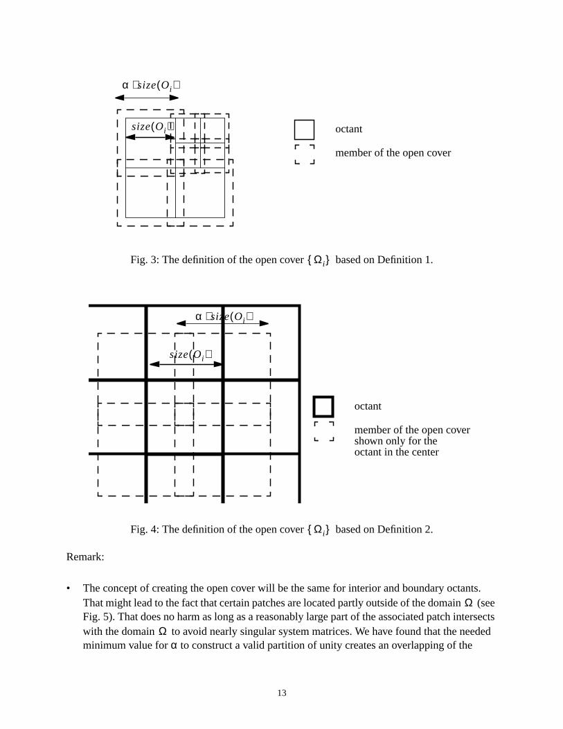
• The concept of creating the open cover will be the same for interior and boundary octanThat might lead to the fact that certain patches are located partly outside of the domainFig. 5). That does no harm as long as a reasonably large part of the associated patch intwith the domain to avoid nearly singular system matrices. We have found that the neminimum value forα to construct a valid partition of unity creates an overlapping of the

octant

member of the open cover

size Oi( )

α size Oi( )⋅

Ωi

octant

member of the open cover

size Oi( )

α size Oi( )⋅

shown only for theoctant in the center

Ωi

Ω

Ω

13

ave to

an inte-

e use

ntage

sented

s inte-

es an

es are

ound-

ently

l

patches with the domain that is large enough.

Fig. 5: Patch located partly outside of the domainΩ.

4. Constructing integration cells based on the octree structure

For the numerical integration of the governing equations, numerical quadrature formulas h

be employed. The most efficient methods, e.g. the Gauss quadrature formula, are based on

gration over a unit domain for which the weights and integration points are tabulated. To mak

of those methods a discretization consisting of simply shaped topological objects is of adva

since it facilitates the definition of the necessary mapping function. Since the spaces repre

by the terminal octants are closed and do not overlap we can use interior terminal octants a

gration cells for the numerical integration scheme. The cubical shape of an octant provid

easy way to map the integration domain onto a unit cube where standard integration rul

applied.

For arbitrary domains we face the problem that boundary octants are cut arbitrarily by the b

ary of the problem domain (see Fig. 2). The domain of integration for that cell is consequ

only the portion of the terminal cell that is interior toΩ. To perform the integration in termina

DomainΩ

Ωi

14

or tri-

t nec-

ndary

ong as

earch-

(1).

ntegra-

t the

g. 7,

n

sume

ls. Fur-

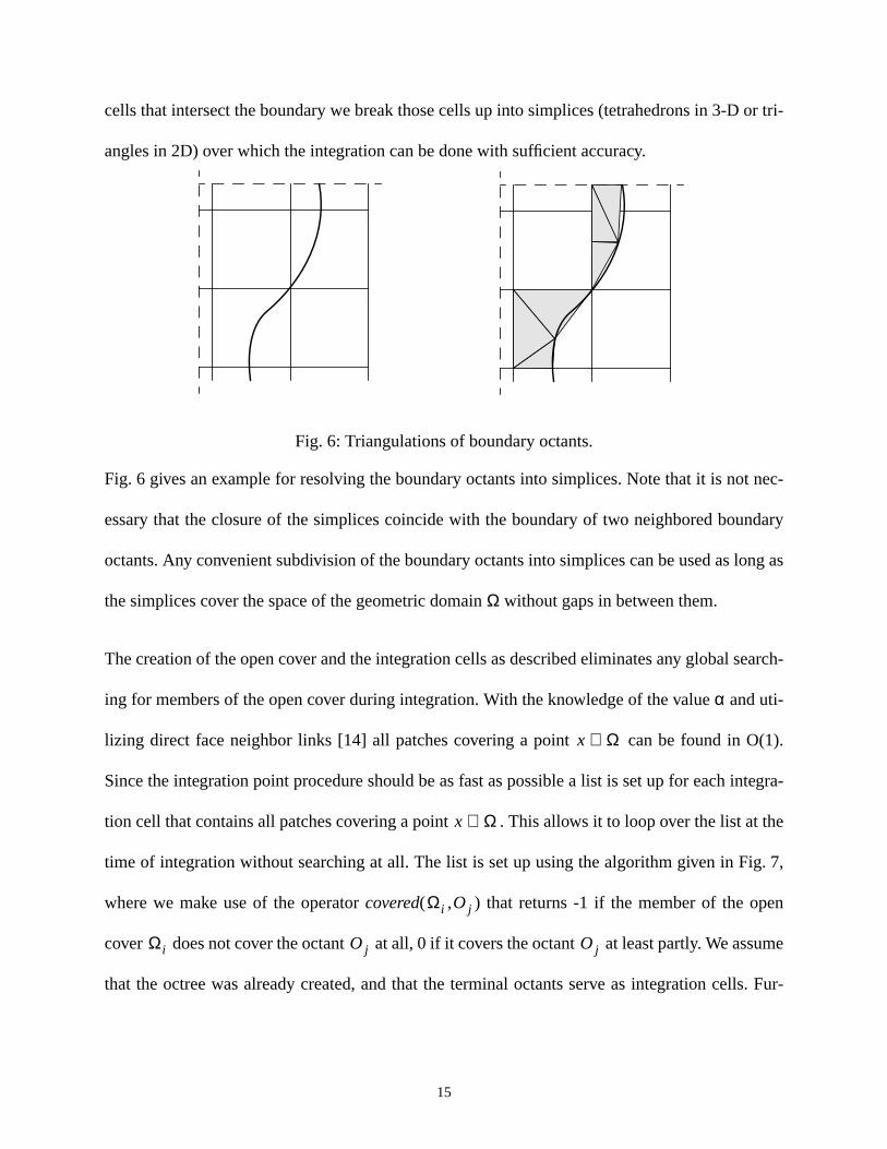
cells that intersect the boundary we break those cells up into simplices (tetrahedrons in 3-D

angles in 2D) over which the integration can be done with sufficient accuracy.

Fig. 6: Triangulations of boundary octants.

Fig. 6 gives an example for resolving the boundary octants into simplices. Note that it is no

essary that the closure of the simplices coincide with the boundary of two neighbored bou

octants. Any convenient subdivision of the boundary octants into simplices can be used as l

the simplices cover the space of the geometric domainΩ without gaps in between them.

The creation of the open cover and the integration cells as described eliminates any global s

ing for members of the open cover during integration. With the knowledge of the valueα and uti-

lizing direct face neighbor links [14] all patches covering a point can be found in O

Since the integration point procedure should be as fast as possible a list is set up for each i

tion cell that contains all patches covering a point . This allows it to loop over the list a

time of integration without searching at all. The list is set up using the algorithm given in Fi

where we make use of the operatorcovered( , ) that returns -1 if the member of the ope

cover does not cover the octant at all, 0 if it covers the octant at least partly. We as

that the octree was already created, and that the terminal octants serve as integration cel

x Ω∈

x Ω∈

Ωi Oj

Ωi Oj Oj

15

d that a

al ele-

aining

avail-

e con-

ing a

ts and

can be

er of

ecting

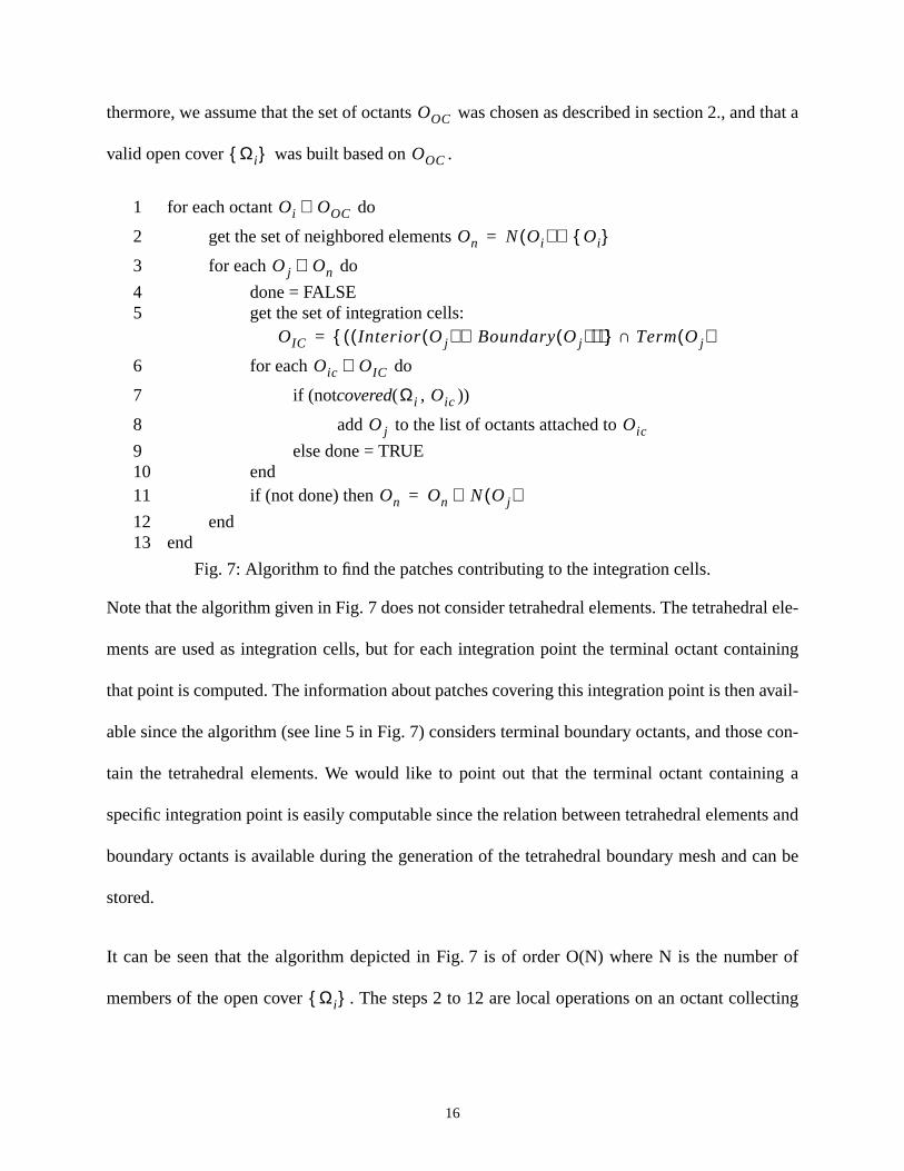
thermore, we assume that the set of octants was chosen as described in section 2., an

valid open cover was built based on .

1 for each octant do

2 get the set of neighbored elements

3 for each do

4 done = FALSE5 get the set of integration cells:

6 for each do

7 if (notcovered( , ))

8 add to the list of octants attached to

9 else done = TRUE10 end11 if (not done) then

12 end13 end

Fig. 7: Algorithm to find the patches contributing to the integration cells.

Note that the algorithm given in Fig. 7 does not consider tetrahedral elements. The tetrahedr

ments are used as integration cells, but for each integration point the terminal octant cont

that point is computed. The information about patches covering this integration point is then

able since the algorithm (see line 5 in Fig. 7) considers terminal boundary octants, and thos

tain the tetrahedral elements. We would like to point out that the terminal octant contain

specific integration point is easily computable since the relation between tetrahedral elemen

boundary octants is available during the generation of the tetrahedral boundary mesh and

stored.

It can be seen that the algorithm depicted in Fig. 7 is of order O(N) where N is the numb

members of the open cover . The steps 2 to 12 are local operations on an octant coll

OOC

Ωi OOC

Oi OOC∈

On N Oi( ) Oi ∪=

Oj On∈

OIC Interior Oj( ) Boundary Oj( )∪( )( ) Term Oj( )∩=

Oic OIC∈

Ωi Oic

Oj Oic

On On N Oj( )∪=

Ωi

16

stant

he

coin-

s the

hat is

ation

m the

the

of the

ble to

m the

hich

of the

ary of

cells.

neighbor information using direct neighbor links. Those operations are performed in con

time assuming an adjusted octree [14].

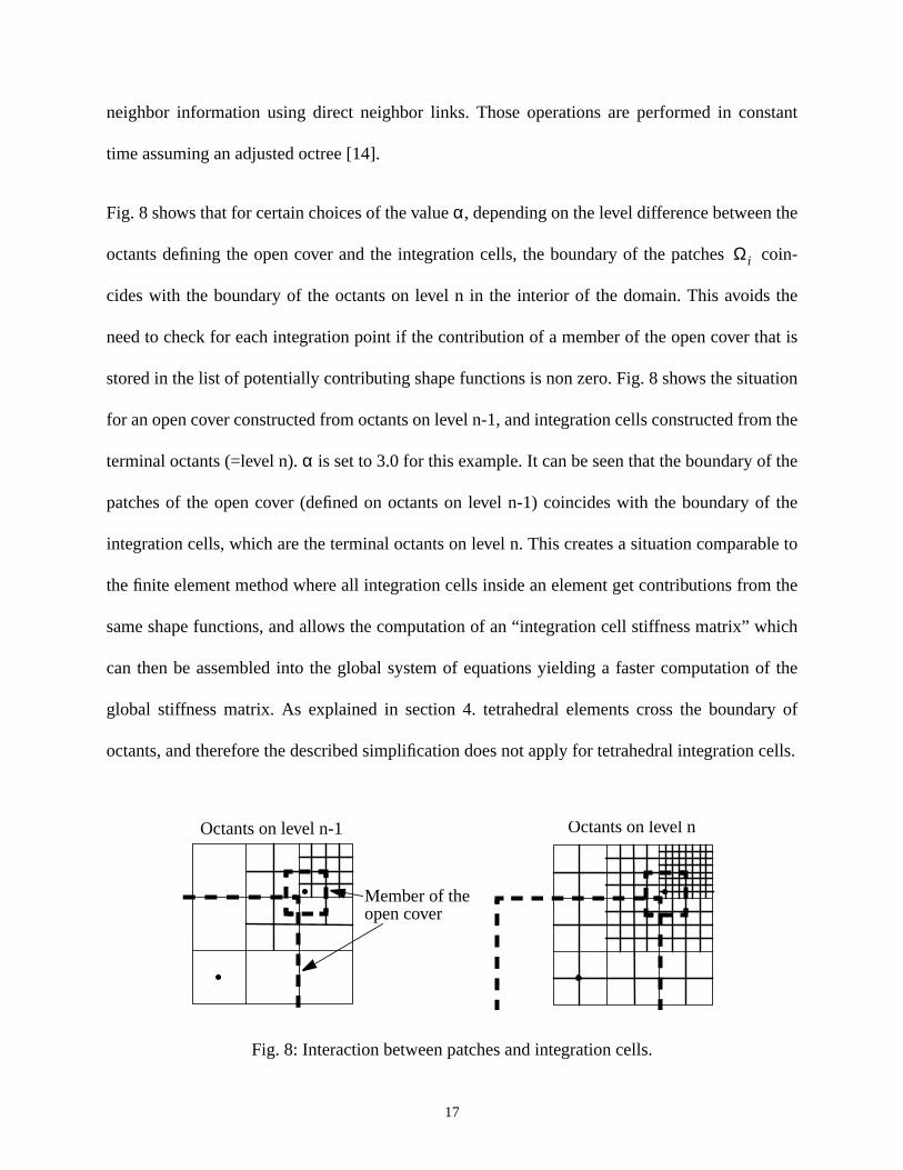
Fig. 8 shows that for certain choices of the valueα, depending on the level difference between t

octants defining the open cover and the integration cells, the boundary of the patches

cides with the boundary of the octants on level n in the interior of the domain. This avoid

need to check for each integration point if the contribution of a member of the open cover t

stored in the list of potentially contributing shape functions is non zero. Fig. 8 shows the situ

for an open cover constructed from octants on level n-1, and integration cells constructed fro

terminal octants (=level n).α is set to 3.0 for this example. It can be seen that the boundary of

patches of the open cover (defined on octants on level n-1) coincides with the boundary

integration cells, which are the terminal octants on level n. This creates a situation compara

the finite element method where all integration cells inside an element get contributions fro

same shape functions, and allows the computation of an “integration cell stiffness matrix” w

can then be assembled into the global system of equations yielding a faster computation

global stiffness matrix. As explained in section 4. tetrahedral elements cross the bound

octants, and therefore the described simplification does not apply for tetrahedral integration

Fig. 8: Interaction between patches and integration cells.

Ωi

Member of theopen cover

Octants on level nOctants on level n-1

17

y that

rking

es will

van-

hape

cells

ple we

s are

ration

ndary.

5. Examples

The focus of this work was on the development of the octree-based discretization technolog

can be used with the various partition of unity methods (like hp-clouds, Element Free Gale

Methods etc.). Simple numerical examples have been done to be sure that the structur

work, and we are currently working on implementing a partition of unity method that takes ad

tage of the discretization not only for the purpose of integration and identifying contributing s

functions, but also as a means to construct the shape functions themselves.

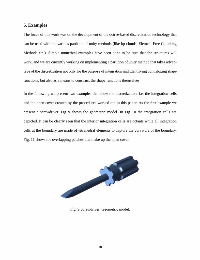
In the following we present two examples that show the discretization, i.e. the integration

and the open cover created by the procedures worked out in this paper. As the first exam

present a screwdriver. Fig. 9 shows the geometric model. In Fig. 10 the integration cell

depicted. It can be clearly seen that the interior integration cells are octants while all integ

cells at the boundary are made of tetrahedral elements to capture the curvature of the bou

Fig. 11 shows the overlapping patches that make up the open cover.

Fig. 9:Screwdriver: Geometric model.

18

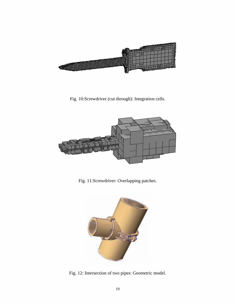
Fig. 10:Screwdriver (cut through): Integration cells.

Fig. 11:Screwdriver: Overlapping patches.

Fig. 12: Intersection of two pipes: Geometric model.

19

r the

the

ry. The

f the

te the

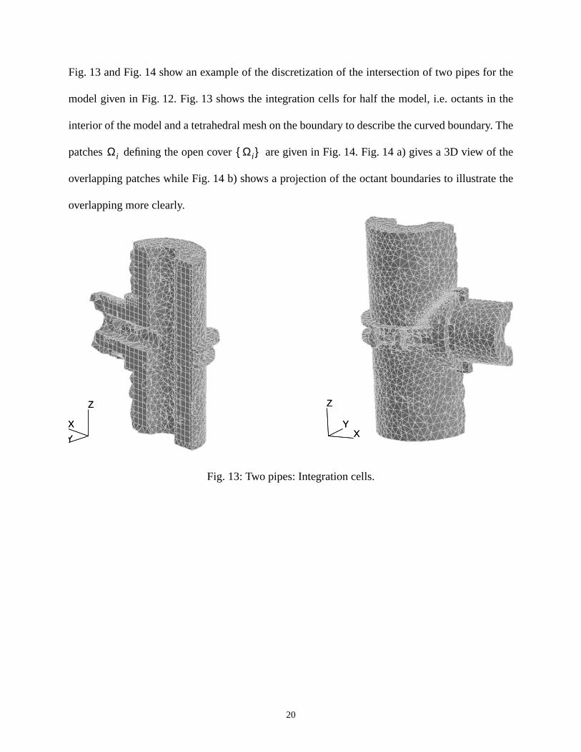
Fig. 13 and Fig. 14 show an example of the discretization of the intersection of two pipes fo

model given in Fig. 12. Fig. 13 shows the integration cells for half the model, i.e. octants in

interior of the model and a tetrahedral mesh on the boundary to describe the curved bounda

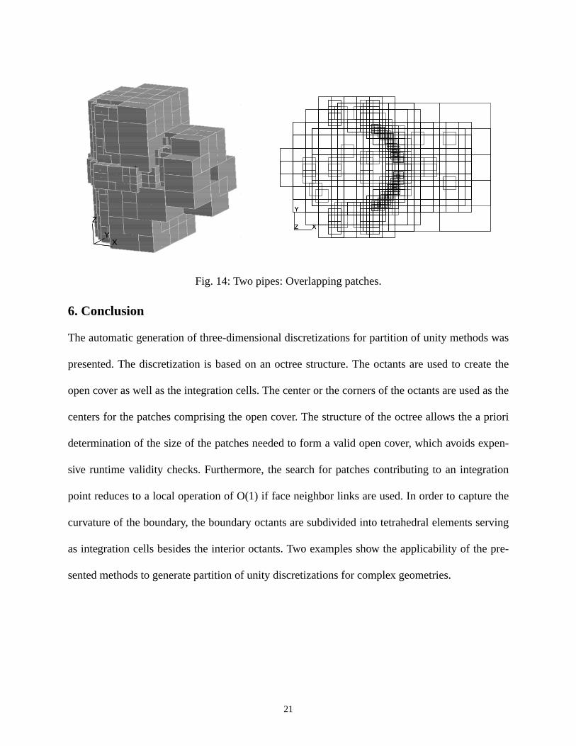
patches defining the open cover are given in Fig. 14. Fig. 14 a) gives a 3D view o

overlapping patches while Fig. 14 b) shows a projection of the octant boundaries to illustra

overlapping more clearly.

Fig. 13: Two pipes: Integration cells.

Ωi Ωi

X

Y

Z

X

Y

Z

XY

Z

XY

Z

20

was

eate the

d as the

priori

xpen-

ration

re the

erving

pre-

Fig. 14: Two pipes: Overlapping patches.

6. Conclusion

The automatic generation of three-dimensional discretizations for partition of unity methods

presented. The discretization is based on an octree structure. The octants are used to cr

open cover as well as the integration cells. The center or the corners of the octants are use

centers for the patches comprising the open cover. The structure of the octree allows the a

determination of the size of the patches needed to form a valid open cover, which avoids e

sive runtime validity checks. Furthermore, the search for patches contributing to an integ

point reduces to a local operation of O(1) if face neighbor links are used. In order to captu

curvature of the boundary, the boundary octants are subdivided into tetrahedral elements s

as integration cells besides the interior octants. Two examples show the applicability of the

sented methods to generate partition of unity discretizations for complex geometries.

XY

Z

XY

ZX

Y

Z X

Y

Z

21

ation

econd5 -

40,

ated

t. J.

th-

and

hreece on

alueat-

thods.

ds.nt of

kin

om-

en-selaer

turepu-

: J. of

7. Acknowledgment

The authors would like to gratefully acknowledge the support of the National Science Found

under grant ASC-9704969.

8. References[1] Babuska, I; Caloz, G; Osborn, JE (1994): Special finite element methods for a class of s

order elliptic problems with rough coefficients. SIAM J. Numerical Analysis, 31(4), 74981.

[2] Babuska, I; Melenk, JM (1997): The Partition of Unity Method. Int. J. Numer. Meth. Eng.727-758.

[3] Baehmann, PL; Shephard, MS (1989): Adaptive multiple level h-refinement in automfinite element analyses, Engng. with Computers 5(3/4),235-247.

[4] Beall, MW; Shephard, MS (1997): A General Topology-Based Mesh Data Structure. InNumer. Meth. Eng. 40, 1573 - 1596.

[5] Belytschko, T; Lu, YY; Gu, L (1994): Element-Free Galerkin Methods. Int. J. Numer. Meods Eng. 37, 229-256.

[6] deCougny, HL; Shephard, MS (1999): Parallel volume meshing using face removalshierarchical repartitioning. Comput. Methods Appl. Mech. Eng. 174(3-4),275-298.

[7] Duarte, CA; Babuska, I; Oden, JT (1998): Generalized Finite Element Methods for TDimensional Structural Mechanics Problems. Proceedings of the International ConferenComputational Engineering Science, Atlanta, October 1998.

[8] Duarte, CA.; Oden, JT (1995): Hp Clouds - A Meshless Method to Solve Boundary-VProblems. TICAM Report 95-05, Texas Institute for Computational and Applied Mathemics. The University of Texas at Austin.

[9] Lancaster, P; Salkauskas, K (1981): Surfaces Generated by Moving Least Squares MeMath. of Comp. Vol 37, Number 155, 141 - 158.

[10] Liu, WK; Li, S; Belytschko, T (1995): Moving Least Square Reproducing Kernel Metho(I) Methodology and Convergence. Technical Report No. Tech-ME-95-3-XX, DepartmeMechanical Engineering, Northwestern University.

[11] Lu, YY; Belytschko, T; Gu, L (1994): A new implementation of the element free Galermethod. Comput. Methods Appl. Mech. Eng. 113, 397 - 414.

[12] Samet, H (1990): Applications of Spacial Data Structures. Addison-Wesley Publishing Cpany.

[13] Simone, ML (1988): A Distributed Octree Structure and Algorithms for Parallel Mesh Geration. Ph.D., Thesis, Scientific Computation Research Center, Report #13-98, RensPolytechnic Institute, Troy, NY.

[14] Simone, ML; Loy, RM; Shephard, MS; Flaherty, JE (1998): A Distributed Octree Strucand Algorithms for Parallel Mesh Generation. SCOREC Report #23 1996, Scientific Comtation Reserach Center, Rensselaer Polytechnic Institute, Troy, NY 12180. Submitted toParallel and Distributed Computing.

22

ion1522.the

of a

ding

a

d.

-

ise a

proxi-

y

[15] Shephard, MS; de Cougny, HL; O’Bara, RM; Beall, MW (1999): Automatic Grid GeneratUsing Spatially-Based Trees. CRC Handbook of Grid Generation. Boca Raton, 1501 -

[16] Yerry, MA; Shephard, MS (1984): Automatic Three-Dimensional Mesh Generation byModified-Octree Technique. Int. J. Numer. Meth. Eng. 20, 1965 - 1990.

9. Appendix A

The partition of unity can be constructed by determining the best approximation

function , where is a Hilbert space with scalar product and the correspon

norm , and is an-dimensional space with the same norm.

Now let be a basis of . Introducing the notation for

vector containing data at theN data points a scalar product can be define

is a squareNxN matrix with positive diagonal elements. Fol

lowing standard arguments we calculate the best approximation

(8)

with

(9)

If is a constant matrix, (8) is a classical, weighted least squares approximation. Otherw

new set of constants has to be computed for each new point where the value of the ap

mation is needed.

By introducing the matrix with its elements we find the partition of unity b

plugging the solution for the coefficients

g x( ) Gn∈

f x( ) V∈ V • •,( )

• • •,( )= Gn V⊆

h1 h, 2 … hn, , Gn u u x1( ) … u xN( ), ,( )T=

u v,( ) x uTW x( )v=

W x( ) diag w1

x( ) … wN

x( ), ,( )=

g x( )

g x( ) aii 1=

n

∑ x( )hi x( )=

ai x( ) hi hj,( ) xi 1=

n

∑ f hj,( ) x j, 1 2 … n, , ,= =

W x( )

ai x( )

A Aij hi hj,( ) x=

ai x( )

23

Free

etize

ng the

e to

f the

rtition

ted.

s on

(10)

into (8)

(11)

The partition of unity as it is developed here is used by Belytschko et. al. [5] in their Element-

Galerkin Method (EFGM). They use the functions directly as the shape functions to discr

the variational form. The polynomial degree of the shape functions is increased by increasi

number of basis functions used to calculate the partition of unity. At this point we would lik

point out that a necessary condition for the matrix to be invertible is

(12)

if m is the degree of the partition of unity. This basically compels us to increase the size o

patches for a p-extension if a fixed number of patches is given. To be able to compute the pa

of unity from the moving least square method the Matrix has to be inver

Therefore it is necessary that the matrix is not singular. We will point out some implication

implementation issues that arise from that condition.

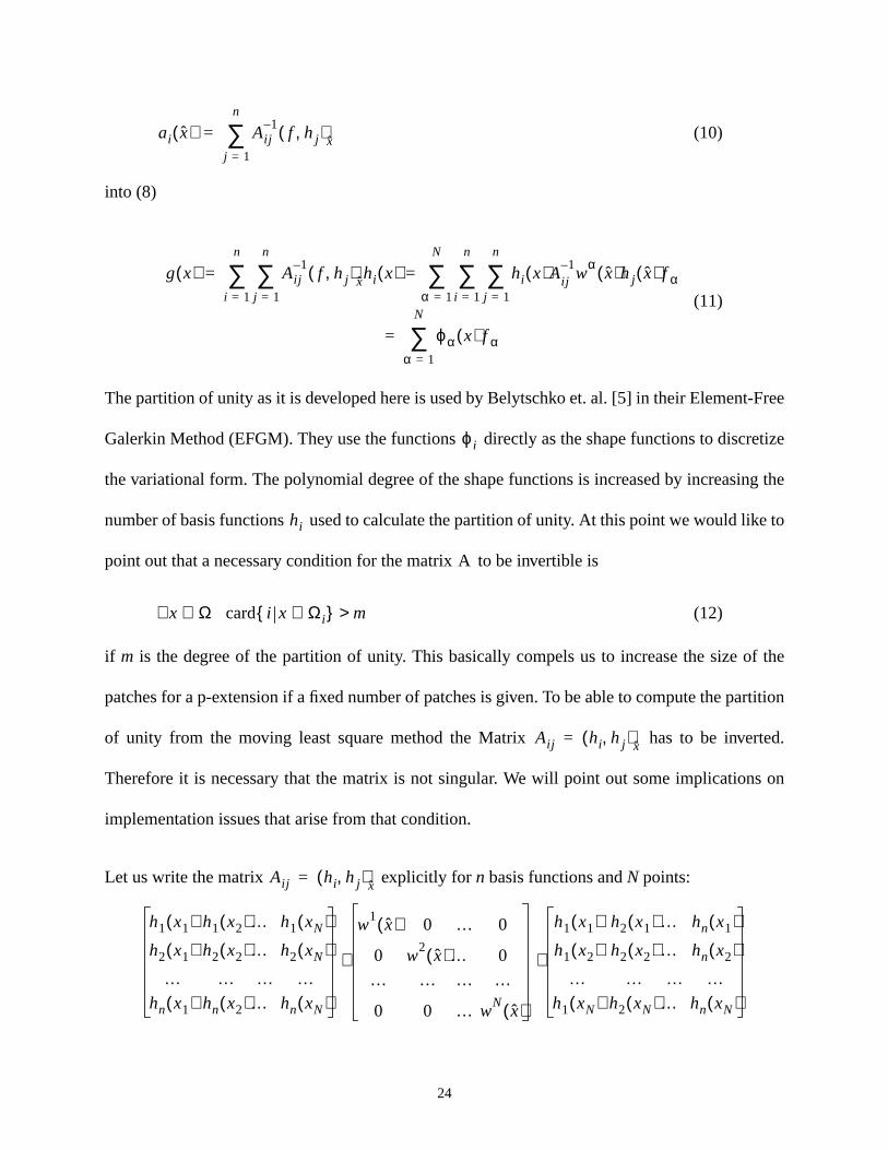
Let us write the matrix explicitly forn basis functions andN points:

ai x( ) Aij1–

f hj,( ) xj 1=

n

∑=

g x( ) Aij1–

f hj,( ) xj 1=

n

∑i 1=

n

∑= hi x( ) hi x( )Aij1–w

αx( )hj x( ) f α

j 1=

n

∑i 1=

n

∑α 1=

N

∑=

ϕα x( ) f αα 1=

N

∑=

ϕi

hi

A

x Ω card i x Ωi∈ m>∈∀

Aij hi hj,( ) x=

Aij hi hj,( ) x=

h1 x1( ) h1 x2( ) … h1 xN( )

h2 x1( ) h2 x2( ) … h2 xN( )

… … … …hn x1( ) hn x2( ) … hn xN( )

w1

x( ) 0 … 0

0 w2

x( ) … 0

… … … …

0 0 … wN

x( )

h1 x1( ) h2 x1( ) … hn x1( )

h1 x2( ) h2 x2( ) … hn x2( )

… … … …h1 xN( ) h2 xN( ) … hn xN( )

⋅ ⋅

24

gate

er-

octree

will

defi-

4

es

ry

of a

yield-

t least

al to

(13)

A necessary condition for the product not to be singular is that . Let us investi

the most critical case . With the theorem (Sylvester Law of Inertia),

if is symmetric and is nonsingular, then and have the same in

tia, i.e. they have the same number of negative, zero and positive eigenvalues.

We conclude thatA is not singular if is not singular, i.e. .

We will now discuss how the regular structure of the center of the patches defined by the

guarantees a priori the non singularity of the product . To simplify the discussion we

look at the 2-dimensional case; an extension to three dimensions is straight forward.

For a constant basis 1 is positive based on the assumption that is positive

nite. For a linear basis 1,x,y, i.e.n = 3 any point in the domain will be covered by at least

patches ifα is chosen appropriately for each patch.α has to be at least 2; it has to be 3 for patch

that are defined on an octant if . The necessa

condition is then fulfilled. Since the center of the 4 patches are given as the corners

square there are always 3 points defining a 2-dimensional simplex, i.e. they are not aligned

ing a positive definite matrix . For a quadratic basis 1,x,y,x*x,x*y,y*yα has to be cho-

sen as 3 or 5, respectively. This will guarantee the coverage of any point in the domain by a

9 patches. This fulfills the necessary condition withn =6 andN = 9. The matrix F would be

singular if for any subset of 6 points coefficients can be found, not all of them equ

zero with

(14)

FWFT

A= =

FWFT

N n≥

N n=

A ℜn n×∈ X ℜn n×∈ A XT

AX

F ℜn n×∈ det F 0≠

FWFT

FWFT

W x( )

Oi Oj∃ N Oi( )∈ Level Oj( ) Level Oi( )<( )

N n≥

FWFT

N n≥

λ1 … λ6, ,

λ1 λ2xi λ3yi λ4xi2 λ5xi yi λ6yi

2+ + + + + 0 i∀ 1…6= =

25

one

point

t an

s dur-

Points that would do so have to lie on a conic section (including a straight line if the c

is degenerated into a cylinder). Obviously, the points given by the octree are representing a 9

stencil pattern, and do not lie on a conic section.

Similar ideas can be employed for a larger basis or a basis in three dimensions to show thaα

can always be chosen that guarantees a non-singular matrix A a priori. Costly computation

ing runtime to perform the check numerically are not necessary.

xi yi,( )

26