A generalized many-facet Rasch model and its Bayesian

Vol.:(0123456789)

Behaviormetrika (2020) 47:469–496https://doi.org/10.1007/s41237-020-00115-7

1 3

INVITED PAPER

A generalized many‑facet Rasch model and its Bayesian estimation using Hamiltonian Monte Carlo

Masaki Uto1 · Maomi Ueno1

Received: 30 September 2019 / Accepted: 9 March 2020 / Published online: 2 May 2020 © The Author(s) 2020

AbstractPerformance assessments, in which raters assess examinee performance for given tasks, have a persistent difficulty in that ability measurement accuracy depends on rater characteristics. To address this problem, various item response theory (IRT) models that incorporate rater characteristic parameters have been proposed. Conven-tional models partially consider three typical rater characteristics: severity, consist-ency, and range restriction. Each are important to improve model fitting and ability measurement accuracy, especially when the diversity of raters increases. However, no models capable of simultaneously representing each have been proposed. One obstacle for developing such a complex model is the difficulty of parameter estima-tion. Maximum likelihood estimation, which is used in most conventional models, generally leads to unstable and inaccurate parameter estimations in complex mod-els. Bayesian estimation is expected to provide more robust estimations. Although it incurs high computational costs, recent increases in computational capabilities and the development of efficient Markov chain Monte Carlo (MCMC) algorithms make its use feasible. We thus propose a new IRT model that can represent all three typi-cal rater characteristics. The model is formulated as a generalization of the many-facet Rasch model. We also develop a Bayesian estimation method for the proposed model using No-U-Turn Hamiltonian Monte Carlo, a state-of-the-art MCMC algo-rithm. We demonstrate the effectiveness of the proposed method through simulation and actual data experiments.

Keywords Item response theory · Many-facet Rasch model · performance assessment · Bayesian estimation · Markov chain Monte Carlo

Communicated by Wim J. van der Linden.

* Masaki Uto [email protected]

Maomi Ueno [email protected]

1 The University of Electro-Communications, Tokyo, Japan

http://crossmark.crossref.org/dialog/?doi=10.1007/s41237-020-00115-7&domain=pdf

470 Behaviormetrika (2020) 47:469–496

1 3

1 Introduction

In various assessment contexts, there is increased need to measure practical, higher order abilities such as problem solving, critical reasoning, and creative thinking skills (e.g., Muraki et al. 2000; Myford and Wolfe 2003; Kassim 2011; Bernardin et al. 2016; Uto and Ueno 2016). To measure such abilities, perfor-mance assessments in which raters assess examinee outcomes or processes for performance tasks have attracted much attention (Muraki et al. 2000; Palm 2008; Wren 2009). Performance assessments have been used in various formats such as essay writing, oral presentations, interview examinations, and group discussions.

In performance assessments, however, difficulty persists in that ability measure-ment accuracy strongly depends on rater and task characteristics, such as rater sever-ity, consistency, range restriction, task difficulty, and discrimination (e.g., Saal et al. 1980; Myford and Wolfe 2003, 2004; Eckes 2005; Kassim 2011; Suen 2014; Shah et al. 2014; Nguyen et al. 2015; Bernardin et al. 2016). Therefore, improving meas-urement accuracy requires ability estimation considering the effects of those charac-teristics (Muraki et al. 2000; Suen 2014; Uto and Ueno 2016).

For this reason, item response theory (IRT) models that incorporate rater and task characteristic parameters have been proposed (e.g., Uto and Ueno 2016; Eckes 2015; Patz and Junker 1999; Linacre 1989). One representative model is the many-facet Rasch model (MFRM) (Linacre 1989). Although several MFRM variations exist (Myford and Wolfe 2003, 2004; Eckes 2015), the most common formation is defined as a rating scale model (RSM) (Andrich 1978) that incorporates rater severity and task difficulty parameters. This model assumes a common interval rating scale for all raters, but it is known that in practice, rating scales vary among raters due to the effects of range restriction, a common rater characteristic indicating the tendency for raters to overuse a limited number of rating categories (Myford and Wolfe 2003; Kassim 2011; Eckes 2005; Saal et al. 1980; Rahman et al. 2017). Therefore, this model does not fit data well when raters with a range restriction exist, lowering abil-ity measurement accuracy. To address this problem, another MFRM formation that relaxes the condition for an equal-interval rating scale for raters has been proposed (Linacre 1989). This model, however, still makes assumptions that might not be sat-isfied, namely a same rating consistency for all raters and same discrimination power for all tasks (Uto and Ueno 2016; Patz et al. 2002). To relax these assumptions, an IRT model that incorporates parameters for rater consistency and task discrimina-tion has also been proposed (Uto and Ueno 2016). Performance declines when raters with range restrictions exist, however, because like conventional MFRM, the model assumes equal interval scales for raters.

The three rater characteristics assumed in the conventional models—sever-ity, range restriction, and consistency—are known to generally occur when rater diversity increases (Myford and Wolfe 2003; Kassim 2011; Eckes 2005; Saal et al. 1980; Uto and Ueno 2016; Rahman et al. 2017; Uto and Ueno 2018a), and ignoring any one will decrease model fitting and measurement accuracy. How-ever, no models capable of simultaneously considering all these characteristics have been proposed so far.

471

1 3

Behaviormetrika (2020) 47:469–496

One obstacle for developing such a model is the difficulty of parameter estima-tion. The MFRM and its extensions conventionally use maximum likelihood esti-mations. However, this generally leads to unstable, inaccurate parameter estima-tions in complex models. For complex models, a Bayesian estimation method called expected a posteriori (EAP) estimation generally provides more robust estima-tions (Uto and Ueno 2016; Fox 2010). EAP estimation involves solutions to high-dimensional multiple integrals, and thus incurs high computational costs, but recent increases in computational capabilities and the development of efficient algorithms such as Markov chain Monte Carlo (MCMC) make it feasible. In IRT studies, EAP estimation using MCMC has been used for hierarchical Bayesian IRT, multidimen-sional IRT, and multilevel IRT (Fox 2010).

We, therefore, propose a new IRT model that can represent all three rater char-acteristics and applies a developed Bayesian estimation method using MCMC. Spe-cifically, the proposed model is formulated as a generalization of the MFRM with-out equal interval rating scales for raters. The proposed model has the following benefits:

1. Model fitting is improved for an increased variety of raters, because the charac-teristics of each rater can be more flexibly represented.

2. More accurate ability measurements will be provided when the variety of raters increases, because abilities can be more precisely estimated considering the effects of each rater’s characteristics.

We also present a Bayesian estimation method for the proposed model using No-U-Turn Hamiltonian Monte Carlo, a state-of-the-art MCMC algorithm (Hoffman and Gelman 2014). We further demonstrate that the method can appropriately estimate model parameters even when the sample size is relatively small, such as the case of 30 examinees, 3 tasks, and 5 raters.

2 Data

This study assumes that performance assessment data X consist of a rating xijr ∈ K = {1, 2,… ,K} assigned by rater r ∈ R = {1, 2,… ,R} to performance of examinee j ∈ J = {1, 2,… , J} for performance task i ∈ I = {1, 2,… , I} . There-fore, data X are described as

where xijr = −1 represents missing data.This study aims to accurately estimate examinee ability from rating data X . In

performance assessments, however, a difficulty persists in that ability measurement accuracy strongly depends on rater and task characteristics (e.g., Saal et al. 1980; Myford and Wolfe 2003; Eckes 2005; Kassim 2011; Suen 2014; Shah et al. 2014; Bernardin et al. 2016; DeCarlo et al. 2011; Crespo et al. 2005).

(1)X = {xijr|xijr ∈ K ∪ {−1}, i ∈ I, j ∈ J, r ∈ R},


1 3

3 Common rater and task characteristics

The following are common rater characteristics on which ability measurement accu-racy generally depends:

1. Severity: The tendency to give consistently lower ratings than are justified by performance.

2. Consistency: The extent to which the rater assigns similar ratings to performances of similar quality.

3. Range restriction: The tendency to overuse a limited number of rating categories. Special cases of range restriction are the central tendency, namely a tendency to overuse the central categories, and the extreme response tendency, a tendency to prefer endpoints of the response scale (Elliott et al. 2009).

The following are typical task characteristics on which accuracy depends:

1. Difficulty: More difficult tasks tend to receive lower ratings.2. Discrimination: The extent to which different levels of the ability to be measured

are reflected in task outcome quality.

To estimate examinee abilities while considering these rater and task characteristics, item response theory (IRT) models that incorporate parameters representing those characteristics have been proposed (e.g., Uto and Ueno 2016; Eckes 2015; Patz and Junker 1999; Linacre 1989). Before introducing these models, the following section describes the conventional IRT model on which they are based.

4 Item response theory

IRT (Lord 1980), which is a test theory based on mathematical models, has been increasingly used with the widespread adoption of computer testing. IRT hypoth-esizes a functional relationship between observed examinee responses to test items and latent ability variables that are assumed to underlie the observed responses. IRT models provide an item response function that specifies the probability of a response to a given item as a function of latent examinee ability and the item’s characteristics. IRT offers the following benefits:

1. It is possible to estimate examinee ability while considering characteristics of each test item.

2. Examinee responses to different test items can be assessed on the same scale.3. Missing data can be easily estimated.

IRT has traditionally been applied to test items for which responses can be scored as correct or incorrect, such as multiple-choice items. In recent years, however, there

473

1 3


have been attempts to apply polytomous IRT models to performance assessments (Muraki et al. 2000; Matteucci and Stracqualursi 2006; DeCarlo et al. 2011). The following subsections describe two representative polytomous IRT models: the gen-eralized partial credit model (GPCM) (Muraki 1997) and the graded response model (GRM) (Samejima 1969).

4.1 Generalized partial credit model

The GPCM gives the probability that examinee j receives score k for test item i as

where �i is a discrimination parameter for item i, �ik is a step difficulty parameter denoting difficulty of transition between scores k − 1 and k in the item, and �j is the latent ability of examinee j. Here, �i1 = 0 for each i is given for model identification.

Decomposing the step difficulty parameter �ik to �i + dik , the GPCM is often described as

where �i is a positional parameter representing the difficulty of item i and dik is a step parameter denoting difficulty of transition between scores k − 1 and k for item i. Here, di1 = 0 and

∑K

k=2dik = 0 for each i are given for model identification.

The GPCM is a generalization of the partial credit model (PCM) (Masters 1982) and the rating scale model (RSM) (Andrich 1978). The PCM is a special case of the GPCM, where �i = 1.0 for all items. Moreover, the RSM is a special case of PCM, where �ik is decomposed to �i + dk . Here, dk is a category parameter that denotes dif-ficulty of transition between categories k − 1 and k.

4.2 Graded response model

The GRM is another polytomous IRT model that has item parameters similar to those of the GPCM. The GRM gives the probability that examinee j obtains score k for test item i as

(2)Pijk =exp

∑k

m=1

��i(�j − �im)

�∑K

l=1exp

∑l

m=1

��i(�j − �im)

� ,

(3)Pijk =exp

∑k

m=1

��i(�j − �i − dim)

�∑K

l=1exp

∑l

m=1

��i(�j − �i − dim)

� ,

(4)Pijk = P∗ijk−1

− P∗ijk,

(5)

⎧⎪⎨⎪⎩

P∗ijk

=1

1+exp (−�i(�j−bik))k = 1,… ,K − 1,

P∗ij0

= 1,

P∗ijK

= 0,


1 3

In these equations, bik is the upper grade threshold parameter for category k of item i, indicating the difficulty of obtaining a category greater than or equal to k for item i. The order of difficulty parameters is bi1 < bi2 < ⋯ < biK−1.

4.3 Interpretation of item parameters

This subsection presents item characteristic parameters based on Eq. (3) form of the GPCM, which has the most item parameters of the models described above.

Figure 1 depicts item response curves (IRCs) of the GPCM for four items with the parameters presented in Table 1, with the horizontal axis showing latent ability � and the vertical axis showing probability Pijk . The IRCs show that examinees with lower (higher) ability tend to obtain lower (higher) scores.

The difficulty parameter �i controls the location of the IRC. As the value of this parameter increases, the IRC shifts to the right. Comparing the IRCs for Item 2 with

−2 −1 0 1 2

Item 1

Ability θ

Prob

abilit

y P i

jk

0.0

0.2

0.4

0.6

0.8

1.0

1.2

k=1k=2

k=3k=4

k=5

−2 −1 0 1 2

Item 2

Ability θ

Prob

abilit

y P i

jk

0.0

0.2

0.4

0.6

0.8

1.0

1.2

k=1k=2

k=3k=4

k=5

−2 −1 0 1 2

Item 3

Ability θ

Prob

abilit

y P i

jk

0.0

0.2

0.4

0.6

0.8

1.0

1.2

k=1k=2

k=3k=4

k=5

−2 −1 0 1 2

Item 4

Ability θ

Prob

abilit

y P i

jk

0.0

0.2

0.4

0.6

0.8

1.0

1.2

k=1k=2

k=3k=4

k=5

Fig. 1 IRCs of the GPCM for four items with different parameters

Table 1 Parameters used in Fig. 1

�i

�i

di2

di3

di4

di5

Item 1 1.5 0.0 −1.5 0.5 0.8 1.2Item 2 1.5 1.5 −1.5 0.5 0.8 1.2Item 3 0.5 0.0 −1.5 0.5 0.8 1.2Item 4 1.5 0.0 −1.5 0.5 0.0 2.0

475

1 3


those for Item 1 shows that obtaining higher scores is more difficult in items with higher difficulty parameter values.

Item discrimination parameter �i controls differences in response probabilities among the rating categories. The IRCs for Item 3 in Fig. 1 show that lower item dis-criminations indicate smaller differences. This trend implies increased randomness of ratings assigned to examinees for low-discrimination items. Low-discrimination items generally lower ability measurement accuracy, because observed data do not necessarily correlate with true ability.

Parameter dik represents the location on the � scale at which the adjacent catego-ries k and k − 1 are equally likely to be observed (Sung and Kang 2006; Eckes 2015). Therefore, when the difference di(k+1) − dik increases, the probability of obtaining category k increases over widely varying ability scales. In Item 4, the response prob-ability for category 4 had a higher value than those for other items, because di5 − di4 is relatively larger.

5 IRT models incorporating rater parameters

As described in Sect. 2, this study applies IRT models to three-way data X com-prising examinees × tasks × raters. However, the models introduced above are not directly applicable to such data. To address this problem, IRT models that incorpo-rate rater characteristic parameters have been proposed (Ueno and Okamoto 2008; Uto and Ueno 2016; Patz et al. 2002; Patz and Junker 1999; Linacre 1989). In these models, item parameters are regarded as task parameters.

The MFRM (Linacre 1989) is the most common IRT model that incorporates rater parameters. The MFRM belongs to the family of Rasch models (Rasch 1980), including the RSM and the PCM introduced in Sect. 4.1. The MFRM has been con-ventionally used for analyzing various performance assessments (e.g., Myford and Wolfe 2003, 2004; Eckes 2005; Saal et al. 1980; Eckes 2015).

Several MFRM variations exist (Myford and Wolfe 2003, 2004; Eckes 2015), but the most common formation is defined as a RSM that incorporates a rater severity parameter. This MFRM provides the probability that rater r responds in category k to examinee j’s performance for task i as

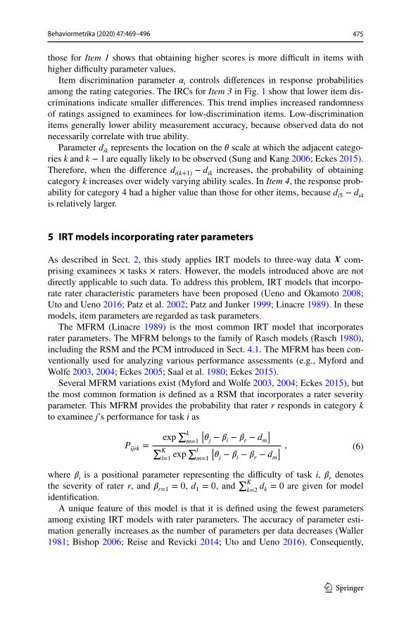
where �i is a positional parameter representing the difficulty of task i, �r denotes the severity of rater r, and �r=1 = 0 , d1 = 0 , and

∑K

k=2dk = 0 are given for model

identification.A unique feature of this model is that it is defined using the fewest parameters

among existing IRT models with rater parameters. The accuracy of parameter esti-mation generally increases as the number of parameters per data decreases (Waller 1981; Bishop 2006; Reise and Revicki 2014; Uto and Ueno 2016). Consequently,

(6)Pijrk =exp

∑k

m=1

��j − �i − �r − dm

�∑K

l=1exp

∑l

m=1

��j − �i − �r − dm

� ,


1 3

this model is expected to provide accurate parameter estimations if it fits well to the given data.

Because it assumes an equal interval scale for raters, however, this model does not fit well to data when rating scales vary across raters, lowering measurement accuracy. Differences in rating scales among raters are typically caused by the effects of range restriction (Myford and Wolfe 2003; Kassim 2011; Eckes 2005; Saal et al. 1980; Rahman et al. 2017). To relax the restriction of equal-interval rating scale for raters, another formation of the MFRM has been proposed (Linacre 1989). That model provides probability Pijrk as

where, drk is the difficulty of transition between categories k − 1 and k for rater r, reflecting how rater r tends to use category k. Here, �r=1 = 0 , dr1 = 0 , and ∑K

k=2drk = 0 are given for model identification. For convenience, we refer to this

model as “rMFRM” below.This model, however, still assumes that rating consistency is the same for all

raters and that all tasks have the same discriminatory power, assumptions that might not be satisfied in practice (Uto and Ueno 2016). To relax these constraints, an IRT model that allows differing rater consistency and task discrimination power has been proposed (Uto and Ueno 2016). The model is formulated as an extension of GRM, and provides the probability Pijrk as

where �i is a discrimination parameter for task i, �r reflects the consistency of rater r, �r represents the severity of rater r, and bik denotes the difficulty of obtaining score k for task i (with bi1 < bi2 < ⋯ < biK−1 ). Here, �r=1 = 1 and �1 = 0 are assumed for model identification. For convenience, we refer to this model as “rGRM” below.

5.1 Interpretation of rater parameters

This subsection describes how the above models represent the typical rater charac-teristics introduced in Sect. 3.

Rater severity is represented as �r in MFRM and rMFRM and as �r in rGRM. The IRC shifts to the right as this parameter values increases, indicating that raters tend to consistently assign low scores. To illustrate this point, Fig. 2 shows IRCs of the MFRM for raters with different severity. Here, we used a low severity value �r = −1.0 for the left panel and a high value �r = 1.0 for the right panel. Other

(7)Pijrk =exp

∑k

m=1

��j − �i − �r − drm

�∑K

l=1exp

∑l

m=1

��j − �i − �r − drm

� ,

(8)

Pijrk = P∗ijrk−1

− P∗ijrk

,

⎧⎪⎨⎪⎩

P∗ijrk

=1

1+exp(−�i�r(�j−bik−�r))k = 1,… ,K − 1,

P∗ijr0

= 1,

P∗ijrK

= 0,

477

1 3


model parameters were the same. Figure 2 shows that the IRC for a severe rater is farther right than that for the lenient rater.

Only rMFRM describes the range restriction characteristic, represented as drk . When dr(k+1) and drk are closer, the probability of responding with category k decreases. Conversely, as the difference dr(k+1) − drk increases, the response prob-ability for category k also increases. Figure 3 shows IRCs of the rMFRM for two raters with different drk values. We used dr2 = −1.5 , dr3 = 0.0 , dr4 = 0.5 , and dr5 = 1.5 for the left panel, and dr2 = −2.0 , dr3 = −1.0 , dr4 = 1.0 , and dr5 = 1.5 for the right panel. The left-side item has relatively larger values of dr3 − dr2 and dr5 − dr4 , thus increasing response probabilities for categories 2 and 4 in the IRC. The right-side item shows that the response probability for category 3 is increased, because dr4 − dr3 has a larger value. The points presented above illustrate that parameter drk reflects the range restriction characteristic.

rGRM represents rater consistency as �r , with lower values indicating smaller differences in response probabilities between the rating categories. This reflects that raters with a lower consistency parameter have stronger tendencies to assign different ratings to examinees with similar ability levels. Figure 4 shows IRCs of rGRM for two raters with different consistency levels. The left panel shows a high

−2 −1 0 1 2Ability θ

Prob

abilit

y P i

jrk

0.0

0.2

0.4

0.6

0.8

1.0

1.2

k=1k=2

k=3k=4

k=5


Prob

abilit

y P i

jrk

0.0

0.2

0.4

0.6

0.8

1.0

1.2

k=1k=2

k=3k=4

k=5

Fig. 2 IRCs of MFRM for two raters with different severity


Prob

abilit

y P i

jrk

0.0

0.2

0.4

0.6

0.8

1.0

1.2

k=1k=2

k=3k=4

k=5


Prob

abilit

y P i

jrk

0.0

0.2

0.4

0.6

0.8

1.0

1.2

k=1k=2

k=3k=4

k=5

Fig. 3 IRCs of rMFRM for two raters with different range restriction characteristics


1 3

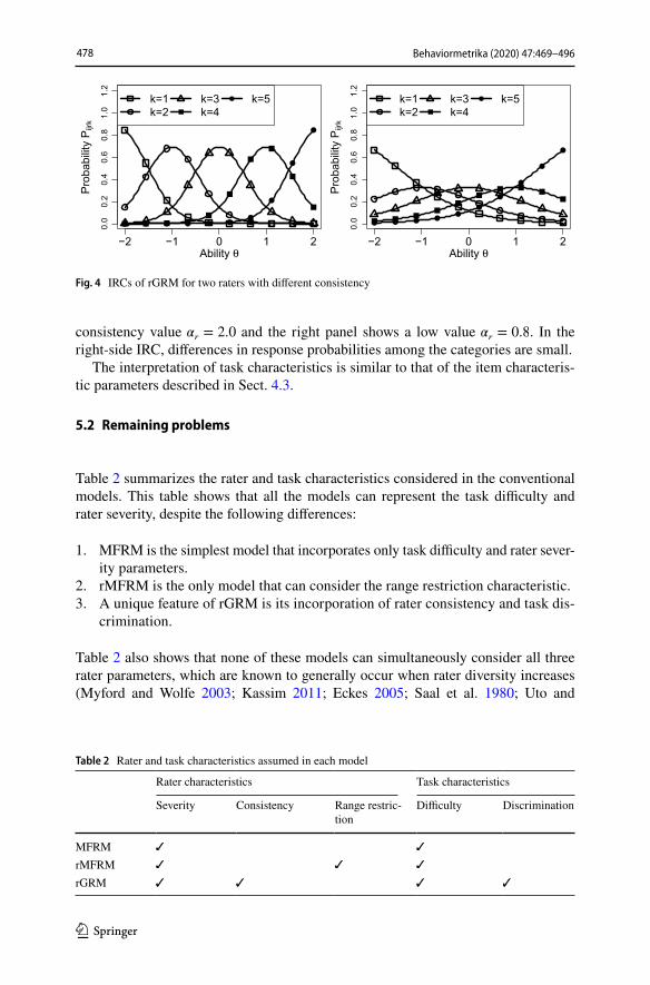
consistency value �r = 2.0 and the right panel shows a low value �r = 0.8 . In the right-side IRC, differences in response probabilities among the categories are small.

The interpretation of task characteristics is similar to that of the item characteris-tic parameters described in Sect. 4.3.

5.2 Remaining problems

Table 2 summarizes the rater and task characteristics considered in the conventional models. This table shows that all the models can represent the task difficulty and rater severity, despite the following differences:

1. MFRM is the simplest model that incorporates only task difficulty and rater sever-ity parameters.

2. rMFRM is the only model that can consider the range restriction characteristic.3. A unique feature of rGRM is its incorporation of rater consistency and task dis-

crimination.

Table 2 also shows that none of these models can simultaneously consider all three rater parameters, which are known to generally occur when rater diversity increases (Myford and Wolfe 2003; Kassim 2011; Eckes 2005; Saal et al. 1980; Uto and


Prob

abilit

y P i

jrk

0.0

0.2

0.4

0.6

0.8

1.0

1.2

k=1k=2

k=3k=4

k=5


Prob

abilit

y P i

jrk

0.0

0.2

0.4

0.6

0.8

1.0

1.2

k=1k=2

k=3k=4

k=5

Fig. 4 IRCs of rGRM for two raters with different consistency

Table 2 Rater and task characteristics assumed in each model

Rater characteristics Task characteristics

Severity Consistency Range restric-tion

Difficulty Discrimination

MFRM ✓ ✓

rMFRM ✓ ✓ ✓

rGRM ✓ ✓ ✓ ✓

479

1 3


Ueno 2016; Rahman et al. 2017; Uto and Ueno 2018a). Thus, ignoring any one will decrease model fitting and ability measurement accuracy. We thus propose a new IRT model that incorporates all three rater parameters.

5.3 Other statistical models for performance assessment

The models described above have been proposed as IRT models that directly incor-porate rater parameters. A different model, the hierarchical rater model (HRM) (Patz et al. 2002; DeCarlo et al. 2011), introduces an ideal rating for each outcome and hierarchical structure data modeling. In the HRM, however, the number of ideal ratings, which should be estimated from given rating data, rapidly increases as the number of examinees or tasks increases. Ability and parameter estimation accura-cies are generally reduced when the number of parameters per data increases. There-fore, accurate estimations under the HRM are more difficult than those for the mod-els introduced above.

Several statistical models similar to the HRM have been proposed without IRT (Piech et al. 2013; Goldin 2012; Desarkar et al. 2012; Ipeirotis et al. 2010; Lauw et al. 2007; Abdel-Hafez and Xu 2015; Chen et al. 2011; Baba and Kashima 2013). However, those models cannot estimate examinee ability, because they do not incor-porate an ability parameter.

From the above, we are not concerned with the models described in this subsection.

6 Proposed model

To address the problems described in Sect. 5.2, we propose a new IRT model that incorporates the three rater characteristic parameters. The proposed model is for-mulated as a rMFRM that incorporates a rater consistency parameter and further incorporates a task discrimination parameter like that in rGRM. Specifically, the proposed model provides the probability that rater r assigns score k to examinee j’s performance for task i as

In the proposed model, rater consistency, severity, and range restriction characteris-tics are, respectively, represented as �r , �r , and drk . Interpretations of these param-eters are as described in Sect. 5.1.

The proposed model entails a non-identifiability problem, meaning that param-eter values cannot be uniquely determined, because different value sets can give same response probability. For the proposed model without task parameters, parameters are identifiable by assuming a specific distribution for the ability and constraining dr1 = 0 and

∑K

k=2drk = 0 for each r, because this is consistent with conventional GPCM in

which item parameters are regarded as rater parameters. However, the proposed model

(9)Pijrk =exp

∑k

m=1

��r�i(�j − �i − �r − drm)

�∑K

l=1exp

∑l

m=1

��r�i(�j − �i − �r − drm)

� ,


1 3

still has indeterminacy of the scale for �r�i and that of the location for �i + �r , even when these constraints are given. Specifically, the response probability Pijrk with �r and �i engenders the same value of Pijrk with ��

r= �rc and ��

i=

�i

c for any constant

c, because ��r��i= (�rc)

�i

c= �r�i . Similarly, the response probability with �i and �r

engenders the same value of Pijrk with ��i= �i + c and ��

r= �r − c for any constant c,

because ��i+ ��

r= (�i + c) + (�r − c) = �i + �r . Scale indeterminacy, as in the �r�i

case, is known to be removable by fixing one parameter or by restricting the product of some parameters (Fox 2010). Furthermore, location indeterminacy, as in the �i + �r case, is solvable by fixing one parameter or by restricting the mean of some param-eters (Fox 2010). This study, therefore, uses the restrictions

∏I

i=1�i = 1 ,

∑I

i=1�i = 0 ,

dr1 = 0 , and ∑K

k=2drk = 0 for model identification, in addition to assuming a specific

distribution for the ability.The proposed model improves model fitting when the variety of raters increases,

because the characteristics of each rater can be more flexibly represented. It also more accurately measures ability when rater variety increases, because it can estimate abil-ity by more precisely reflecting rater characteristics. Note that ability measurement is improved only when the decrease in model misfit by increasing parameters exceeds the increase in parameter estimation errors caused by the decrease in data per parameter. This property is known as the bias–accuracy tradeoff (van der Linden 2016a).

7 Parameter estimation

This section presents the parameter estimation method for the proposed model.Marginal maximum likelihood estimation using an EM algorithm is a common

method for estimating IRT model parameters (Baker and Kim 2004). However, for complex models like that used in this study, EAP estimation, a form of Bayesian esti-mation, is known to provide more robust estimations (Uto and Ueno 2016; Fox 2010).

EAP estimates are calculated as the expected value of the marginal posterior distri-bution of each parameter (Fox 2010; Bishop 2006). The posterior distribution in the proposed model is

where

Therein, �j = {�j ∣ j ∈ J} , log�i = {log �i ∣ i ∈ I} , �i = {�i ∣ i ∈ I} , log�r= {log �

r∣ r

∈ R} , �r = {�r ∣ r ∈ R} , and drk = {drk ∣ r ∈ R, k ∈ K} . Here, g(S��S) =

∏s∈S g(s��S)

(10)

g(�j, log�i, log�r, �i, �r, drk|X)∝ L(X|�j, log�i, log�r, �i, �r, drk)g(�j|��)g(log�i|��i)g(log�r|��r )g(�i|��i)g(�r|��r )g(drk|�d),

(11)L(X|�j, log�i, log�r, �i, �r, drk) = ΠJj=1

ΠIi=1

ΠRr=1

ΠKk=1

(Pijrk)zijrk ,

(12)zijrk =

{1 ∶ xijr = k,

0 ∶ otherwise.

481

1 3


(where S is a set of parameters) indicates a prior distribution. �s is a hyperparameter for parameter s, which is arbitrarily determined to reflecting analyst’s subjectivity.

The marginal posterior distribution for each parameter is derived marginalizing across all parameters except the target one. For a complex IRT model, however, it is generally infeasible to derive the marginal posterior distribution or to calcu-late it using numerical analysis methods such as the Gaussian quadrature integral, because doing so requires solutions to high-dimensional multiple integrals. MCMC, a random sampling-based estimation method, can be used to address this problem. The effectiveness of MCMC has been demonstrated in various fields (Bishop 2006; Brooks et al. 2011; Uto et al. 2017; Louvigné et al. 2018). In IRT studies, MCMC has been used for complex models such as hierarchical Bayesian IRT, multidimen-sional IRT, and multilevel IRT (Fox 2010; Uto 2019).

7.1 MCMC algorithm

The Metropolis-Hastings-within-Gibbs sampling method (Gibbs/MH) (Patz and Junker 1999) has been commonly used as a MCMC algorithm for parameter estima-tion in IRT models. The algorithm is simple and easy to implement (Patz and Junker 1999; Zhang et al. 2011; Cai 2010), but it requires long times to converge to the target distribution, because it explores the parameter space via an inefficient random walk (Hoffman and Gelman 2014; Girolami and Calderhead 2011).

The Hamiltonian Monte Carlo (HMC) is an alternative MCMC algorithm with high efficiency (Brooks et al. 2011). Generally, HMC quickly converges to a tar-get distribution in complex high-dimensional problems if two hand-tuned param-eters, namely step size and simulation length, are appropriately selected (Neal 2010; Hoffman and Gelman 2014; Girolami and Calderhead 2011). In recent years, the No-U-Turn (NUT) sampler (Hoffman and Gelman 2014), an extension of HMC that eliminates hand-tuned parameters, has been proposed. The “Stan” software pack-age (Carpenter et al. 2017) makes implementation of a NUT-based HMC easy. This algorithm has thus recently been used for parameter estimations in various statistical models, including IRT models (Luo and Jiao 2018; Jiang and Carter 2019).

We, therefore, use a NUT-based MCMC algorithm for parameter estimations in the proposed model. The estimation program was implemented in RStan (Stan Development Team 2018). The developed Stan code is provided in an Appen-dix. In this study, the prior distributions are set as �j , log �i , log �r , �i , �r , and drk ∼ N(0.0, 1.02) , where N(�, �2) is a normal distribution with mean � and standard deviation � . Furthermore, we calculate EAP estimates as the mean of parameter samples obtained from 500 to 1000 periods of three independent MCMC chains.

7.2 Accuracy of parameter recovery

This subsection evaluates parameter recovery accuracy under the proposed model using the MCMC algorithm. The experiments were conducted as follows:


1 3

1. Randomly generate true parameters for the proposed model from the distributions described in Sect. 7.1.

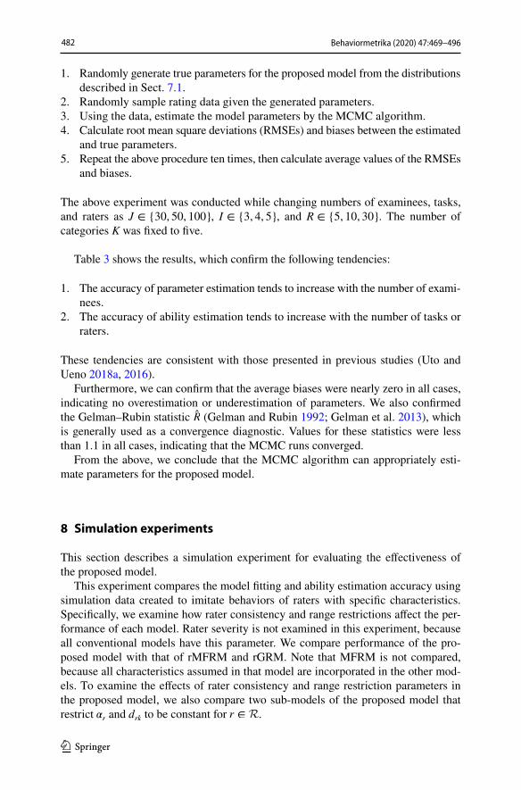
2. Randomly sample rating data given the generated parameters.3. Using the data, estimate the model parameters by the MCMC algorithm.4. Calculate root mean square deviations (RMSEs) and biases between the estimated

and true parameters.5. Repeat the above procedure ten times, then calculate average values of the RMSEs

and biases.

The above experiment was conducted while changing numbers of examinees, tasks, and raters as J ∈ {30, 50, 100} , I ∈ {3, 4, 5} , and R ∈ {5, 10, 30} . The number of categories K was fixed to five.

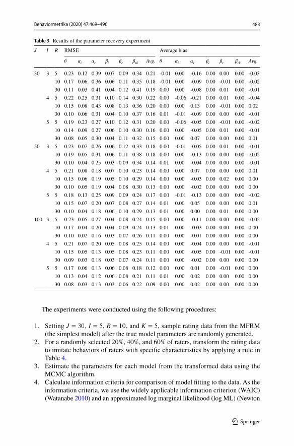
Table 3 shows the results, which confirm the following tendencies:

1. The accuracy of parameter estimation tends to increase with the number of exami-nees.

2. The accuracy of ability estimation tends to increase with the number of tasks or raters.

These tendencies are consistent with those presented in previous studies (Uto and Ueno 2018a, 2016).

Furthermore, we can confirm that the average biases were nearly zero in all cases, indicating no overestimation or underestimation of parameters. We also confirmed the Gelman–Rubin statistic R̂ (Gelman and Rubin 1992; Gelman et al. 2013), which is generally used as a convergence diagnostic. Values for these statistics were less than 1.1 in all cases, indicating that the MCMC runs converged.

From the above, we conclude that the MCMC algorithm can appropriately esti-mate parameters for the proposed model.

8 Simulation experiments

This section describes a simulation experiment for evaluating the effectiveness of the proposed model.

This experiment compares the model fitting and ability estimation accuracy using simulation data created to imitate behaviors of raters with specific characteristics. Specifically, we examine how rater consistency and range restrictions affect the per-formance of each model. Rater severity is not examined in this experiment, because all conventional models have this parameter. We compare performance of the pro-posed model with that of rMFRM and rGRM. Note that MFRM is not compared, because all characteristics assumed in that model are incorporated in the other mod-els. To examine the effects of rater consistency and range restriction parameters in the proposed model, we also compare two sub-models of the proposed model that restrict �r and drk to be constant for r ∈ R.

483

1 3


The experiments were conducted using the following procedures:

1. Setting J = 30 , I = 5 , R = 10 , and K = 5 , sample rating data from the MFRM (the simplest model) after the true model parameters are randomly generated.

2. For a randomly selected 20%, 40%, and 60% of raters, transform the rating data to imitate behaviors of raters with specific characteristics by applying a rule in Table 4.

3. Estimate the parameters for each model from the transformed data using the MCMC algorithm.

4. Calculate information criteria for comparison of model fitting to the data. As the information criteria, we use the widely applicable information criterion (WAIC) (Watanabe 2010) and an approximated log marginal likelihood (log ML) (Newton

Table 3 Results of the parameter recovery experiment

J I R RMSE Average bias

� �i

�r

�i

�r

�rk

Avg. � �i

�r

�i

�r

�rk

Avg.

30 3 5 0.23 0.12 0.39 0.07 0.09 0.34 0.21 -0.01 0.00 -0.16 0.00 0.00 0.00 -0.0310 0.17 0.06 0.36 0.06 0.11 0.35 0.18 -0.01 0.00 -0.09 0.00 -0.01 0.00 -0.0230 0.11 0.03 0.41 0.04 0.12 0.41 0.19 0.00 0.00 -0.08 0.00 0.01 0.00 -0.01

4 5 0.22 0.25 0.31 0.10 0.14 0.30 0.22 0.00 -0.06 -0.21 0.00 0.01 0.00 -0.0410 0.15 0.08 0.43 0.08 0.13 0.36 0.20 0.00 0.00 0.13 0.00 -0.01 0.00 0.0230 0.10 0.06 0.31 0.04 0.10 0.37 0.16 0.01 -0.01 -0.09 0.00 0.00 0.00 -0.01

5 5 0.19 0.23 0.27 0.10 0.12 0.31 0.20 0.00 -0.06 -0.05 0.00 -0.01 0.00 -0.0210 0.14 0.09 0.27 0.06 0.10 0.30 0.16 0.00 0.00 -0.05 0.00 0.01 0.00 -0.0130 0.08 0.05 0.30 0.04 0.11 0.32 0.15 0.00 0.00 0.07 0.00 0.00 0.00 0.01

50 3 5 0.23 0.07 0.26 0.06 0.12 0.33 0.18 0.00 -0.01 -0.05 0.00 0.01 0.00 -0.0110 0.19 0.05 0.31 0.06 0.11 0.38 0.18 0.00 0.00 -0.13 0.00 0.00 0.00 -0.0230 0.10 0.04 0.25 0.03 0.09 0.34 0.14 0.01 0.00 -0.04 0.00 0.00 0.00 -0.01

4 5 0.21 0.08 0.18 0.07 0.10 0.23 0.14 0.00 0.00 0.07 0.00 0.00 0.00 0.0110 0.15 0.06 0.19 0.05 0.10 0.29 0.14 0.00 0.00 -0.03 0.00 0.02 0.00 0.0030 0.10 0.05 0.19 0.04 0.08 0.30 0.13 0.00 0.00 -0.02 0.00 0.00 0.00 0.00

5 5 0.18 0.13 0.25 0.09 0.09 0.24 0.17 0.00 -0.01 -0.13 0.00 0.00 0.00 -0.0210 0.15 0.07 0.20 0.07 0.08 0.27 0.14 0.01 0.00 0.05 0.00 0.00 0.00 0.0130 0.10 0.04 0.18 0.06 0.10 0.29 0.13 0.01 0.00 0.00 0.00 0.01 0.00 0.00

100 3 5 0.23 0.05 0.27 0.04 0.08 0.24 0.15 0.00 0.00 -0.11 0.00 0.00 0.00 -0.0210 0.17 0.04 0.20 0.04 0.09 0.24 0.13 0.01 0.00 -0.03 0.00 0.00 0.00 0.0030 0.10 0.02 0.16 0.03 0.07 0.26 0.11 0.00 0.00 -0.01 0.00 0.00 0.00 0.00

4 5 0.21 0.07 0.20 0.05 0.08 0.25 0.14 0.00 0.00 -0.04 0.00 0.00 0.00 -0.0110 0.15 0.05 0.13 0.05 0.08 0.23 0.11 0.00 0.00 -0.05 0.00 -0.01 0.00 -0.0130 0.09 0.03 0.18 0.03 0.07 0.24 0.11 0.00 0.00 -0.02 0.00 0.00 0.00 0.00

5 5 0.17 0.06 0.13 0.06 0.08 0.18 0.12 0.00 0.00 0.01 0.00 -0.01 0.00 0.0010 0.13 0.04 0.12 0.06 0.08 0.21 0.11 0.01 0.00 0.02 0.00 0.00 0.00 0.0030 0.08 0.03 0.13 0.03 0.06 0.22 0.09 0.00 0.00 0.02 0.00 0.00 0.00 0.00


1 3

and Raftery 1994), which have previously been used for IRT model comparison (Uto and Ueno 2016; Reise and Revicki 2014; van der Linden 2016b). Note that we use an approximate log ML (Newton and Raftery 1994), which is calculated as the harmonic mean of likelihoods sampled during MCMC, because exact cal-culation of ML is intractable due to the high-dimensional integrals involved. The model minimizing criteria scores is regarded as the optimal model. After ordering the models by each information criterion, calculate the rank of each model.

5. To evaluate the accuracy of ability estimation, calculate the RMSE and the correla-tion between true ability values and ability estimates as calculated from the trans-formed data in Procedure 8. Note that the RMSE was calculated after standardizing both the true and the estimated ability values, because the scale of ability differs between the MFRM from which the true values generated and a target model.

6. Repeat the above procedures ten times, then calculate the average rank and cor-relation.

Tables 5 and 6 show the results. In these tables, bold text represents highest val-ues for ranks, correlations, and lowest RMSEs, and underlined text represents the next good values. The results show that the model performance strongly depends on whether the model can represent rater characteristics appearing in the assess-ment process. Specifically, the following findings were obtained from the results:

• For data with rating behavior pattern (A), in which raters with lower consist-ency exist, the models with rater consistency parameter �r (namely, rGRM and the proposed model with or without the constraint drk ) tend to fit well and pro-vide high ability estimation accuracy.

• For data with rating behavior pattern (B), in which raters with range restric-tions exist, the models with the drk parameter (namely, rMFRM and the pro-posed model with or without the constraint �r ) provide high performance.

• For data with rating behavior pattern (C), in which both raters with range restriction and those with low consistency exist, the proposed model provides the highest performance, because it is the only model that incorporates both rater parameters.

These results confirm that the proposed model provides better model fitting and more accurate ability estimations than do the conventional models when assuming

Table 4 Rules for creating rating data that imitate behaviors of raters with specific characteristics

Behavior pattern Transformation procedure

(A) Low consistency 50% of rater ratings are changed to randomly selected rating categories(B) Strong range restriction After randomly selecting two categories k′ and k′′ , where k′ < X̄r ≤ k′′

( X̄r is the average of ratings by rater r), 50% of the ratings are changed to k′ if the rating is less than X̄r and to k′′ otherwise

(C) Both behaviors Both the above transformation rules are simultaneously applied

485

1 3


varying rater characteristics. Furthermore, these results demonstrate that rater parameters �r and drk appropriately reflect rater consistency and range restriction characteristics, as expected.

9 Actual data experiments

This section describes actual data experiments performed to evaluate performance of the proposed model.

9.1 Actual data

This experiment uses rating data obtained from a peer assessment activity among university students. We selected this situation because it is a typical example in which the existence of raters with various characteristics can be assumed (e.g., Nguyen et al. 2015; Uto and Ueno 2018b; Uto et al. n.d.). We gathered actual peer assessment data through the following procedures:

Table 5 Results of model comparison using information criteria (Values in parentheses are the standard deviation of the rank)

Rate of Behavior Proposed model rMFRM rGRM

changed data pattern No restriction drk

fixed �r fixed

WAIC20% (A) 1.7 (0.5) 1.3 (0.5) 4.4 (0.5) 4.6 (0.5) 3.0 (0.0)

(B) 2.2 (1.0) 3.8 (0.6) 2.2 (0.8) 1.8 (0.9) 5.0 (0.0)(C) 1.1 (0.3) 2.1 (0.6) 4.3 (0.7) 4.1 (0.7) 3.4 (1.2)

40% (A) 1.4 (0.5) 1.6 (0.5) 4.4 (0.5) 4.6 (0.5) 3.0 (0.0)(B) 1.8 (0.9) 4.0 (0.0) 2.4 (0.7) 1.8 (0.8) 5.0 (0.0)(C) 1.0 (0.0) 2.5 (1.0) 4.4 (0.7) 3.4 (0.5) 3.7 (1.3)

60% (A) 1.1 (0.3) 1.9 (0.3) 4.2 (0.4) 4.0 (0.9) 3.8 (1.0)(B) 1.8 (0.9) 4.0 (0.0) 2.4 (0.7) 1.8 (0.8) 5.0 (0.0)(C) 1.0 (0.0) 3.8 (0.6) 3.1 (0.3) 2.1 (0.3) 5.0 (0.0)

log ML20% (A) 1.2 (0.4) 1.8 (0.4) 4.4 (0.5) 4.6 (0.5) 3.0 (0.0)

(B) 1.2 (0.4) 3.9 (0.3) 2.4 (0.5) 2.5 (1.0) 5.0 (0.0)(C) 1.0 (0.0) 2.2 (0.4) 4.4 (0.7) 4.0 (0.7) 3.4 (1.2)

40% (A) 1.0 (0.0) 2.0 (0.0) 4.5 (0.5) 4.5 (0.5) 3.0 (0.0)(B) 1.0 (0.0) 4.0 (0.0) 2.5 (0.5) 2.5 (0.5) 5.0 (0.0)(C) 1.0 (0.0) 2.5 (1.0) 4.3 (0.7) 3.5 (0.5) 3.7 (1.4)

60% (A) 1.0 (0.0) 2.0 (0.0) 4.3 (0.5) 3.9 (0.9) 3.8 (1.0)(B) 1.2 (0.4) 4.0 (0.0) 2.3 (0.8) 2.5 (0.5) 5.0 (0.0)(C) 1.0 (0.0) 3.8 (0.6) 3.0 (0.5) 2.2 (0.4) 5.0 (0.0)


1 3

1. Subjects were 34 university students majoring in various STEM fields, including statistics, materials, chemistry, engineering, robotics, and information science.

2. Subjects were asked to complete four essay-writing tasks from the National Assessment of Educational Progress (NAEP) assessments in 2002 and 2007 (Per-sky et al. 2003; Salahu-Din et al. 2008). No specific or preliminary knowledge was needed to complete these tasks.

3. After the subjects completed all tasks, they were asked to evaluate the essays of other subjects for all four tasks. These assessments were conducted using a rubric based on assessment criteria for grade 12 NAEP writing (Salahu-Din et al. 2008), consisting of five rating categories with corresponding scoring criteria.

In this experiment, we also collected rating data that simulate behaviors of raters with specific characteristics. Specifically, we gathered ten other university students and asked them to evaluate the 134 essays written by the initial 34 sub-jects following the instructions in Table 7. The first three raters are expected to provide inconsistent ratings, the next four raters to imitate raters with a range restriction, and the last three raters to simulate severe or lenient raters. For sim-plicity, hereinafter we refer to such raters as controlled raters.

We evaluate the effectiveness of the proposed model using these data.

Table 6 Accuracy of ability estimation in the simulation experiment

Rate of Behavior Proposed model rMFRM rGRM

changed data pattern No restriction drk

fixed �r fixed

RMSE20% (A) 0.1277 0.1287 0.1557 0.1518 0.1444

(B) 0.1285 0.1309 0.1282 0.1254 0.1389(C) 0.1508 0.1483 0.1863 0.1846 0.1651

40% (A) 0.1585 0.1578 0.2177 0.2146 0.1679(B) 0.1332 0.1386 0.1321 0.1361 0.1522(C) 0.1760 0.1810 0.2450 0.2432 0.1934

60% (A) 0.1793 0.1798 0.2606 0.2588 0.2005(B) 0.1520 0.1582 0.1542 0.1542 0.1790(C) 0.2112 0.2169 0.2944 0.2908 0.2539

Correlation20% (A) 0.9913 0.9912 0.9872 0.9878 0.9888

(B) 0.9912 0.9908 0.9912 0.9916 0.9894(C) 0.9878 0.9883 0.9814 0.9818 0.9854

40% (A) 0.9869 0.9870 0.9751 0.9758 0.9851(B) 0.9907 0.9900 0.9907 0.9903 0.9878(C) 0.9831 0.9822 0.9673 0.9679 0.9790

60% (A) 0.9829 0.9827 0.9643 0.9646 0.9787(B) 0.9877 0.9864 0.9872 0.9873 0.9826(C) 0.9765 0.9752 0.9541 0.9554 0.9660

487

1 3


9.2 Example of parameter estimates

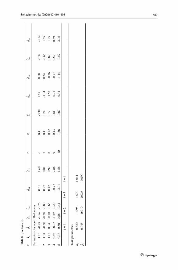
This subsection presents an example of parameter estimation using the proposed model. From the rating data from peer raters and controlled raters, we used the MCMC algorithm to estimate parameters for the proposed model. Table 8 shows the estimated rater and task parameters.

Table 8 confirms the existence of peer raters with various rater characteristics. Figure 5 shows IRCs for four representative peer raters with different character-istics. Here, Rater 17 and Rater 24 are example lenient and inconsistent raters, respectively. Rater 4 and Rater 32 are raters with different range restriction char-acteristics. Specifically, Rater 4 tended to overuse categories k = 2 and k = 4 , and Rater 32 tended to overuse only k = 4.

We can also confirm that the controlled raters followed the provided instruc-tions. Specifically, high severity values are estimated for controlled raters 8 and 9, and a low value is assigned to controlled rater 10, as expected. Figure 5 also shows the IRCs of controlled raters 4, 5, 6, and 7, which confirm range restriction characteristics complying with the instructions. Although we expected raters 1, 2, and 3 to be inconsistent, because they need to perform assessments within a short time, their consistencies were not low.

Table 8 also shows that the tasks had different discrimination powers and dif-ficulty values. However, parameter differences among tasks are smaller than those among raters.

This suggests that the proposed model is suitable for the data, because various rater characteristics are likely to exist.

9.3 Model comparison using information criteria

This subsection presents model comparisons using information criteria. We cal-culated WAIC and log ML for each model using the peer-rater data and the data with controlled rater data.

Table 9 shows the results, with bold text indicating minimum scores. The table shows that the proposed model presents lowest values for both information cri-teria and for both datasets, suggesting that the proposed model is the best model for the actual data. The table also shows that performance of the proposed model

Table 7 Instructions given to ten raters to obtain responses for specific characteristics

Rater Index Instruction

1, 2, 3 Grade essays after quickly reading each essay (within 15 s)4 Assign categories 2 and 4 for more than half of essays5 Assign categories 1 and 4 for more than half of essays6 Assign categories 1 and 5 for more than half of essays7 Assign categories 1, 2, and 4 for more than half of essays8, 9 Grade strictly to decrease the average score10 Grade leniently to increase the average score


1 3

Tabl

e 8

Par

amet

er e

stim

ates

r𝛼r

𝛽r

d̂r2

d̂r3

d̂r4

d̂r5

r𝛼r

𝛽r

d̂r2

d̂r3

d̂r4

d̂r5

Para

met

ers f

or p

eer r

ater

s1

0.78

-0.3

2-1

.35

-0.0

40.

171.

2118

1.52

-0.0

5-1

.20

-0.2

30.

371.

062

0.70

-0.1

0-0

.26

-0.5

6-0

.14

0.96

191.

710.

00-1

.93

-0.2

21.

320.

833

1.60

0.10

-0.7

4-0

.18

0.32

0.59

201.

310.

40-1

.27

-0.5

50.

161.

664

1.04

-0.1

6-1

.53

-0.3

60.

061.

8421

0.69

-0.2

4-1

.04

0.08

0.52

0.44

50.

80-0

.52

-1.7

3-0

.30

0.70

1.33

221.

440.

04-1

.67

-0.3

30.

591.

416

0.90

-0.3

0-1

.60

-0.1

40.

361.

3823

0.96

0.01

-1.4

8-1

.32

0.84

1.95

70.

710.

52-0

.42

-0.4

40.

740.

1224

0.48

-0.0

1-1

.16

-0.6

80.

791.

058

1.76

0.05

-1.3

4-0

.55

0.63

1.27

250.

73-0

.34

-0.5

80.

050.

210.

319

1.15

0.50

-1.6

1-0

.10

0.30

1.41

260.

790.

13-0

.77

-0.5

00.

370.

8910

0.74

-0.3

3-0

.42

-0.1

40.

140.

4227

0.73

-0.6

3-1

.71

-0.2

20.

921.

0011

0.98

-0.4

0-1

.18

-0.6

10.

491.

3028

1.35

-0.2

3-1

.31

-0.1

40.

441.

0012

0.95

-0.3

9-1

.61

-0.5

90.

541.

6529

0.82

-0.3

6-0

.75

-0.6

50.

700.

7013

0.82

0.36

-1.0

5-0

.11

0.48

0.67

300.

460.

52-1

.19

0.17

0.14

0.88

140.

810.

01-1

.74

-0.0

90.

561.

2831

0.80

-0.2

7-0

.92

0.08

-0.3

41.

1715

1.43

-0.3

2-1

.37

-0.6

60.

511.

5332

0.73

-0.6

0-0

.53

-0.9

9-0

.34

1.85

161.

12-0

.01

-0.0

1-1

.59

-0.2

71.

8733

1.30

-0.1

2-1

.14

-0.2

50.

430.

9617

1.17

-0.5

6-1

.08

-0.7

60.

461.

3734

0.81

-0.4

6-1

.47

0.65

-0.1

10.

93

489

1 3


Tabl

e 8

(con

tinue

d)

r𝛼r

𝛽r

d̂r2

d̂r3

d̂r4

d̂r5

r𝛼r

𝛽r

d̂r2

d̂r3

d̂r4

d̂r5

Para

met

ers f

or c

ontro

lled

rate

rs1

1.16

-0.2

8-1

.54

-0.7

60.

611.

696

0.41

-0.3

81.

680.

50-0

.32

-1.8

62

1.34

-0.6

0-0

.28

-0.8

00.

270.

817

0.41

0.24

-1.3

40.

34-0

.65

1.65

31.

180.

04-0

.70

-0.6

80.

420.

978

0.72

0.77

-1.5

8-0

.56

0.89

1.25

40.

98-0

.07

-1.8

9-0

.20

-0.7

72.

869

0.43

0.81

-0.7

1-0

.77

0.59

0.89

50.

360.

800.

86-0

.41

-2.0

11.

5610

1.56

-0.6

7-0

.34

-1.1

4-0

.57

2.05

i=1

i=2

i=3

i=4

Task

par

amet

ers

𝛼i

0.82

01.

095

1.07

01.

041

𝛽i

0.04

50.

019

0.02

6-0

.090


1 3

decreases when the effects of rater consistency or range restriction are ignored, indicating that simultaneous consideration of both is important.

The experimental results show that the proposed model can improve the model fit-ting when raters with various characteristics exist. This is because consistency and range restriction characteristics differ among raters, as described in the previous subsection, and because the proposed model appropriately represents these effects (Fig. 6).

9.4 Accuracy of ability estimation

This subsection compares ability measurement accuracies using the actual data. Spe-cifically, we evaluate how well ability estimates are correlated when abilities are esti-mated using data from different raters. If a model appropriately reflects rater character-istics, ability values estimated from data from different raters will be highly correlated. We thus conducted the following experiment for each model and for two datasets, namely, the peer rater data and the data with controlled rater data:

1. Use MCMC to estimate model parameters.2. Randomly select 5 or 10 ratings assigned to each examinee, then change unse-

lected ratings to missing data.3. Using the dataset with missing data, estimate examinee abilities � given the rater

and task parameters estimated in Procedure 1.4. Repeat the above procedure 100 times, then calculate the correlation between each

pair of ability estimates obtained in Procedure 3. Then, calculate the average and standard deviation of the correlations.

For comparison, we conducted the same experiment using a method in which the true score is given as the average rating. We designate this as the average score method. We also conducted multiple comparisons using Dunnett’s test to ascer-tain whether correlation values under the proposed model are significantly higher than those under the other models.

−2 −1 0 1 2

Rater 17

Ability θ

Prob

abilit

y P i

jrk

0.0

0.2

0.4

0.6

0.8

1.0

1.2

k=1k=2k=3

k=4k=5

−2 −1 0 1 2

Rater 24

Ability θ

Prob

abilit

y P i

jrk

0.0

0.2

0.4

0.6

0.8

1.0

1.2

k=1k=2k=3

k=4k=5

−2 −1 0 1 2

Rater 4

Ability θ

Prob

abilit

y P i

jrk

0.0

0.2

0.4

0.6

0.8

1.0

1.2

k=1k=2k=3

k=4k=5

−2 −1 0 1 2

Rater 32

Ability θ

Prob

abilit

y P i

jrk

0.0

0.2

0.4

0.6

0.8

1.0

1.2

k=1k=2k=3

k=4k=5

Fig. 5 IRCs for four representative peer raters with different characteristics

491

1 3


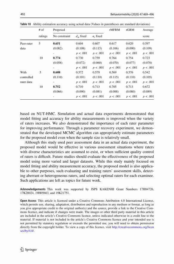
Table 10 shows the results. The results show that all IRT models provide higher correlation values than does the averaged score, indicating that the IRT models effectively improve the accuracy of ability measurements. The results also show that the proposed model provides significantly higher correlations than do the other models, indicating that the proposed model most accurately estimates abilities. We can also confirm that performance of the proposed model rapidly decreases when the effects of rater consistency or range restriction are ignored, suggesting the effectiveness of considering both characteristics to improve accuracy.

These results demonstrate that the proposed model provides the most accurate ability estimations when a large variety of rater characteristics is assumed.

10 Conclusion

We proposed a generalized MFRM that incorporates parameters for three common rater characteristics, namely, severity, range restriction, and consistency. To address the difficulty of parameter estimation under such a complex model, we presented a Bayesian estimation method for the proposed model using a MCMC algorithm

−2 −1 0 1 2

Controlled Rater 4

Ability θ

Prob

abilit

y P i

jrk

0.0

0.2

0.4

0.6

0.8

1.0

1.2

k=1k=2k=3

k=4k=5

−2 −1 0 1 2

Controlled Rater 5

Ability θ

Prob

abilit

y P i

jrk

0.0

0.2

0.4

0.6

0.8

1.0

1.2

k=1k=2k=3

k=4k=5

−2 −1 0 1 2

Controlled Rater 6

Ability θ

Prob

abilit

y P i

jrk

0.0

0.2

0.4

0.6

0.8

1.0

1.2

k=1k=2k=3

k=4k=5

−2 −1 0 1 2

Controlled Rater 7

Ability θ

Prob

abilit

y P i

jrk

0.0

0.2

0.4

0.6

0.8

1.0

1.2

k=1k=2k=3

k=4k=5

Fig. 6 IRCs for controlled raters with strong range restriction

Table 9 Model comparison using actual data

Proposed rMFRM rGRM

No constraint drk

fixed �r fixed

Peer-rater WAIC 11384.58 11492.09 11400.85 11401.92 11471.67data log ML 11200.32 11380.25 11216.18 11242.64 11350.67With controlled WAIC 14489.56 14817.64 14535.58 14547.59 14696.86rater data log ML 14265.97 14683.99 14342.82 14352.92 14559.81


1 3

based on NUT-HMC. Simulation and actual data experiments demonstrated that model fitting and accuracy for ability measurements is improved when the variety of raters increases. We also demonstrated the importance of each rater parameter for improving performance. Through a parameter recovery experiment, we demon-strated that the developed MCMC algorithm can appropriately estimate parameters for the proposed model even when the sample size is relatively small.

Although this study used peer assessment data in an actual data experiment, the proposed model would be effective in various assessment situations where raters with diverse characteristics are assumed to exist, or when sufficient quality control of raters is difficult. Future studies should evaluate the effectiveness of the proposed model using more varied and larger datasets. While this study mainly focused on model fitting and ability measurement accuracy, the proposed model is also applica-ble to other purposes, such evaluating and training raters’ assessment skills, detect-ing aberrant or heterogeneous raters, and selecting optimal raters for each examinee. Such applications are left as topics for future work.

Acknowledgements This work was supported by JSPS KAKENHI Grant Numbers 17H04726, 17K20024, 19H05663, and 19K21751.

Open Access This article is licensed under a Creative Commons Attribution 4.0 International License, which permits use, sharing, adaptation, distribution and reproduction in any medium or format, as long as you give appropriate credit to the original author(s) and the source, provide a link to the Creative Com-mons licence, and indicate if changes were made. The images or other third party material in this article are included in the article’s Creative Commons licence, unless indicated otherwise in a credit line to the material. If material is not included in the article’s Creative Commons licence and your intended use is not permitted by statutory regulation or exceeds the permitted use, you will need to obtain permission directly from the copyright holder. To view a copy of this licence, visit http://creat iveco mmons .org/licen ses/by/4.0/.

Table 10 Ability estimation accuracy using actual data (Values in parentheses are standard deviations)

# of Proposed rMFRM rGRM Average

ratings No constraint drk

fixed �r fixed score

Peer-rater 5 0.651 0.604 0.607 0.617 0.620 0.597data (0.082) (0.108) (0.115) (0.106) (0.090) (0.109)

- p < .001 p < .001 p < .001 p < .001 p < .001

10 0.774 0.730 0.759 0.764 0.754 0.723(0.058) (0.072) (0.060) (0.070) (0.077) (0.070)- p < .001 p < .001 p < .001 p < .001 p < .001

With 5 0.608 0.572 0.579 0.569 0.576 0.542controlled (0.110) (0.101) (0.110) (0.115) (0.110) (0.105)rater data - p < .001 p < .001 p < .001 p < .001 p < .001

10 0.752 0.710 0.713 0.705 0.713 0.672(0.066) (0.090) (0.081) (0.088) (0.080) (0.089)- p < .001 p < .001 p < .001 p < .001 p < .001

http://creativecommons.org/licenses/by/4.0/

http://creativecommons.org/licenses/by/4.0/

493

1 3


Appendix

Stan code for the proposed model.


1 3

References

Abdel-Hafez A, Xu Y (2015) Exploiting the beta distribution-based reputation model in recommender system. In: Proceedings of 28th Australasian joint conference, advances in artificial intelligence. Cham, pp 1–13

Andrich D (1978) A rating formulation for ordered response categories. Psychometrika 43(4):561–573Baba Y, Kashima H (2013) Statistical quality estimation for general crowdsourcing tasks. In: Proceed-

ings of the 19th ACM SIGKDD international conference on knowledge discovery and data mining. ACM, New York, NY, USA, pp 554–562

Baker F, Kim SH (2004) Item response theory: parameter estimation techniques. Marcel Dekker, New York

Bernardin HJ, Thomason S, Buckley MR, Kane JS (2016) Rater rating-level bias and accuracy in perfor-mance appraisals: the impact of rater personality, performance management competence, and rater accountability. Human Resour Manag 55(2):321–340

Bishop CM (2006) Pattern recognition and machine learning (information science and statistics). Springer, Berlin

Brooks S, Gelman A, Jones G, Meng X (2011) Handbook of markov chain Monte Carlo. CRC Press, Boca Raton

Cai L (2010) High-dimensional exploratory item factor analysis by a Metropolis-Hastings Robbins-Monro algorithm. Psychometrika 75(1):33–57

Carpenter B, Gelman A, Hoffman M, Lee D, Goodrich B, Betancourt M, Riddell A (2017) Stan: a proba-bilistic programming language. J Stat Softw Articles 76(1):1–32

Chen B-C, Guo J, Tseng B, Yang J (2011) User reputation in a comment rating environment. In: Proceed-ings of the 17th ACM SIGKDD international conference on knowledge discovery and data mining, pp 159–167

Crespo RM, Pardo A, Pérez JPS, Kloos CD (2005) An algorithm for peer review matching using student profiles based on fuzzy classification and genetic algorithms. In: Proceedings of 18th international conference on industrial and engineering applications of artificial intelligence and expert systems, pp 685–694

DeCarlo LT, Kim YK, Johnson MS (2011) A hierarchical rater model for constructed responses, with a signal detection rater model. J Educ Meas 48(3):333–356

Desarkar MS, Saxena R, Sarkar S (2012) Preference relation based matrix factorization for recommender systems. In: Proceedings of 20th international conference on user modeling, adaptation, and person-alization, pp 63–75

Eckes T (2005) Examining rater effects in TestDaF writing and speaking performance assessments: a many-facet Rasch analysis. Lang Assess Q 2(3):197–221

Eckes T (2015) Introduction to many-facet Rasch measurement: Analyzing and evaluating rater-mediated assessments. Peter Lang Pub. Inc., New York

Elliott M, Haviland A, Kanouse D, Hambarsoomian K, Hays R (2009) Adjusting for subgroup differences in extreme response tendency in ratings of health care: impact on disparity estimates. Health Serv Res 44:542–561

Fox J-P (2010) Bayesian item response modeling: theory and applications. Springer, BerlinGelman A, Carlin J, Stern H, Dunson D, Vehtari A, Rubin D (2013) Bayesian data analysis, 3rd edn.

Taylor & Francis, New YorkGelman A, Rubin DB (1992) Inference from iterative simulation using multiple sequences. Stat Sci

7(4):457–472Girolami M, Calderhead B (2011) Riemann manifold Langevin and Hamiltonian Monte Carlo methods. J

R Stat Soc Ser B (Stat Methodol) 73(2):123–214Goldin IM (2012) Accounting for peer reviewer bias with Bayesian models. In: Proceedings of the work-

shop on intelligent support for learning groups at the 11th international conference on intelligent tutoring systems

Hoffman MD, Gelman A (2014) The No-U-turn sampler: adaptively setting path lengths in Hamiltonian Monte Carlo. J Mach Learn Res 15:1593–1623

Ipeirotis PG, Provost F, Wang J (2010) Quality management on amazon mechanical turk. In: Proceedings of the ACM SIGKDD workshop on human computation, pp 64–67

Jiang Z, Carter R (2019) Using Hamiltonian Monte Carlo to estimate the log-linear cognitive diagnosis model via Stan. Behav Res Methods 51(2):651–662

495

1 3


Kassim NLA (2011) Judging behaviour and rater errors: an application of the many-facet Rasch model. GEMA Online J Lang Stud 11(3):179–197

Lauw WH, Lim E-p, Wang K (2007) Summarizing review scores of “unequal” reviewers. In: Proceedings of the SIAM international conference on data mining

Linacre J (1989) Many-faceted Rasch measurement. MESA Press, San DiegoLord F (1980) Applications of item response theory to practical testing problems. Erlbaum Associates,

New JerseyLouvigné S, Uto M, Kato Y, Ishii T (2018) Social constructivist approach of motivation: social media

messages recommendation system. Behaviormetrika 45(1):133–155Luo Y, Jiao H (2018) Using the Stan program for Bayesian item response theory. Educ Psychol Meas

78(3):384–408Masters G (1982) A Rasch model for partial credit scoring. Psychometrika 47(2):149–174Matteucci M, Stracqualursi L (2006) Student assessment via graded response model. Statistica

66:435–447Muraki E (1997) A generalized partial credit model. In: van der Linden WJ, Hambleton RK (eds) Hand-

book of modern item response theory. Springer, Berlin, pp 153–164Muraki E, Hombo C, Lee Y (2000) Equating and linking of performance assessments. Appl Psychol

Meas 24:325–337Myford CM, Wolfe EW (2003) Detecting and measuring rater effects using many-facet Rasch measure-

ment: Part I. J Appl Meas 4:386–422Myford CM, Wolfe EW (2004) Detecting and measuring rater effects using many-facet Rasch measure-

ment: Part II. J Appl Meas 5:189–227Neal RM (2010) MCMC using Hamiltonian dynamics. Handb Markov Chain Monte Carlo 54:113–162Newton M, Raftery A (1994) Approximate Bayesian inference by the weighted likelihood bootstrap. J R

Stat Soc Ser B Methodol 56(1):3–48Nguyen T, Uto M, Abe Y, Ueno M (2015) Reliable peer assessment for team project based learning using

item response theory. In: Proceedings of international conference on computers in education, pp 144–153

Palm T (2008) Performance assessment and authentic assessment: a conceptual analysis of the literature. Pract Assess Res Eval 13(4):1–11

Patz RJ, Junker B (1999) Applications and extensions of MCMC in IRT: multiple item types, missing data, and rated responses. J Educ Behav Stat 24(4):342–366

Patz RJ, Junker BW, Johnson MS, Mariano LT (2002) The hierarchical rater model for rated test items and its application to largescale educational assessment data. J Educ Behav Stat 27(4):341–384

Persky H, Daane M, Jin Y (2003) The nation’s report card: Writing 2002 (Tech. Rep.). National Center for Education Statistics

Piech C, Huang J, Chen Z, Do C, Ng A, Koller D (2013) Tuned models of peer assessment in MOOCs. In: Proceedings of of sixth international conference of MIT’s learning international networks consortium

Rahman AA, Ahmad J, Yasin RM, Hanafi NM (2017) Investigating central tendency in competency assessment of design electronic circuit: analysis using many facet Rasch measurement (MFRM). Int J Inf Educ Technol 7(7):525–528

Rasch G (1980) Probabilistic models for some intelligence and attainment tests. The University of Chi-cago Press, Chicago

Reise SP, Revicki DA (2014) Handbook of item response theory modeling: applications to typical perfor-mance assessment. Routledge, Abingdon

Saal F, Downey R, Lahey M (1980) Rating the ratings: assessing the psychometric quality of rating data. Psychol Bull 88(2):413–428

Salahu-Din D, Persky H, Miller J (2008) The nation’s report card: writing 2007 (Tech. Rep.). National Center for Education Statistics

Samejima F (1969) Estimation of latent ability using a response pattern of graded scores. Psychom Mon-ogr 17:1–100

Shah NB, Bradley J, Balakrishnan S, Parekh A, Ramchandran K, Wainwright MJ (2014) Some scaling laws for MOOC assessments. ACM KDD workshop on data mining for educational assessment and feedback

Stan Development Team (2018) RStan: the R interface to stan. R package version 2.17.3. http://mc-stan.org

http://mc-stan.org

http://mc-stan.org


1 3

Suen H (2014) Peer assessment for massive open online courses (MOOCs). Int Rev Res Open Distrib Learn 15(3):313–327

Sung HJ, Kang T (2006) Choosing a polytomous IRT model using Bayesian model selection methods. National Council on Measurement in Education Annual Meeting, PP 1–36

Ueno M, Okamoto T (2008) Item response theory for peer assessment. In: Proceedings of IEEE interna-tional conference on advanced learning technologies, pp 554–558

Uto M (2019) Rater-effect IRT model integrating supervised LDA for accurate measurement of essay writing ability. In: Proceedings of international conference on artificial intelligence in education, pp 494–506

Uto M, Louvigné S, Kato Y, Ishii T, Miyazawa Y (2017) Diverse reports recommendation system based on latent Dirichlet allocation. Behaviormetrika 44(2):425–444

Uto M, Nguyen D, Ueno M (n.d.). Group optimization to maximize peer assessment accuracy using item response theory and integer programming. IEEE Trans Learn Technol (in press)

Uto M, Ueno M (2016) Item response theory for peer assessment. IEEE Trans Learn Technol 9(2):157–170

Uto M, Ueno M (2018a) Empirical comparison of item response theory models with rater’s parameters. Heliyon Elsevier 4(5):1–32

Uto M, Ueno M (2018b) Item response theory without restriction of equal interval scale for rater’s score. In: Proceedings of international conference on artificial intelligence in education, pp 363–368

van der Linden WJ (2016a) Handbook of item response theory, volume one: models. CRC Press, Boca Raton

van der Linden WJ (2016b) Handbook of item response theory, volume two: statistical tools. CRC Press, Boca Raton

Waller MI (1981) A procedure for comparing logistic latent trait models. J Educ Meas 18(2):119–125Watanabe S (2010) Asymptotic equivalence of Bayes cross validation and widely applicable information

criterion in singular learning theory. J Mach Learn Res 20:3571–3594Wren GD (2009) Performance assessment: a key component of a balanced assessment system (Tech. Rep.

No. 2). Report from the Department of Research, Evaluation, and AssessmentZhang A, Xie X, You S, Huang X (2011) Item response model parameter estimation based on Bayesian

joint likelihood langevin MCMC method with open software. Int J Adv Comput Technol 3(6):48

Publisher’s Note Springer Nature remains neutral with regard to jurisdictional claims in published maps and institutional affiliations.

Documents

A generalized many-facet Rasch model and its Bayesian