Ecological Modelling, 42 (1988) 125-154 125 Elsevier Science Publishers B.V., Amsterdam - Printed in The Netherlands

A GENERAL MODEL OF FOREST ECOSYSTEM PROCESSES FOR REGIONAL APPLICATIONS I. HYDROLOGIC BALANCE, CANOPY GAS EXCHANGE AND PRIMARY PRODUCTION PROCESSES

STEVEN W. RUNNING and JOSEPH C. COUGHLAN

School of Forestry, University of Montana, Missoula, MT 59812 (U.S.A.)

(Accepted 18 November 1987)

ABSTRACT

Running, S.W. and Coughlan, J.C., 1988. A general model of forest ecosystem processes for regional applications. I. Hydrologic balance, canopy gas exchange and primary production processes. Ecol. Modelling, 42: 125-154.

An ecosystem process model is described that calculates the carbon, water and nitrogen cycles through a forest ecosystem. The model, FOREST-BGC, treats canopy interception and evaporation, transpiration, photosynthesis, growth and maintenance respiration, carbon alloc- ation above and below-ground, litterfall, decomposition and nitrogen mineralization. The model uses leaf area index (LA0 to quantify the forest structure important for energy and mass exchange, and this represents a key simplification for regional scale applications. FOREST-BGC requires daily incoming short-wave radiation, air temperature, dew point, and precipitation as driving variables. The model was used to simulate the annual hydrologic balance and net primary production of a hypothetical forest stand in seven contrasting environments across North America for the year 1984. Hydrologic partitioning ranged from 14/86/0% for evaporation, transpiration and outflow, respectively, in Fairbanks, AK (annual precipitation of 313 mm) to 10/27/66% in Jacksonville, FL (annual ppt of 1244 mm), and these balances changed as LAI was increased from 3 to 9 in successive simulations. Net primary production (Nee) ranged from 0.0 t C ha -1 year -1 at Tucson, AZ, to 14.1 t C ha- year- ~ at Knoxville, TN and corresponded reasonably with observed values at each site. The sensitivity of ecosystem processes to varying LAI in different climates was substantial, and underscores the utility of parameterizing this model at regional scales in the future with forest LAI measurements derived from satellite imagery.

INTRODUCTION

Many of the most pressing ecological questions being asked today address ecosystem processes at regional to global scales. Concerns on the effects of global climate change, global CO 2 increase, regional air pollution, and

0304-3800/88/$03.50 © 1988 Elsevier Science Publishers B.V.

126

regional shifts in vegetation cover on forest processes all require calculations of ecosystem processes at scales much larger than have previously been considered by ecosystem process models. Fundamental requirements in these ecological questions are the rates and controls of energy, carbon, water and nutrient exchange by vegetated surfaces, and the responses of these surfaces to some of the perturbations described above. Most ecosystem process models have been built from and used to simulate the dynamics of a study plot, often 10 m × 10 m or less in size. Some watershed models have been built to calculate hydrologic variables at larger scales, but they do not treat ecological processes. A number of global models have been developed, particularly for global carbon, but they are primarily static budgets that do not mechanistically treat processes, and are not driven by data for specific sites or conditions.

We present here a new model that calculates key processes involved in the carbon, water and nitrogen cycles for forests. The model treats canopy interception and evaporation, transpiration, photosynthesis, growth and maintenance respiration, carbon allocation above and below-ground, litter- fall, decomposition and nitrogen mineralization mechanistically, but in a general way incorporating minimal species-specific data. The model repre- sents a conscious compromise between mechanistic detail and simplifying generality that will allow it to be implemented for regional-scale ecological research.

Additionally, the model was designed to be driven ultimately by remote sensing inputs of surface climate and vegetation structure, in the framework of a geographic information system containing topographic and physical site characteristics (Peterson et al., 1985). Recent workshops on global ecological issues have identified leaf area index (LAI) as the most important single variable for measuring vegetation structure over large areas, and relating it to energy and mass exchange. (Wittwer, 1983; Botkin, 1986). LAI of natural vegetation has been successfully estimated from satellite resolution sensors (Asrar et al., 1984; Running et al., 1986). Consequently, this model is designed to be particularly sensitive to LAI, and LAI is used as the principal independent variable for calculating canopy interception, transpiration, res- piration, photosynthesis, carbon allocation and litterfall.

This paper covers the logic and development of the model FOREST-BGC (BioGeochemical Cycles), and a first exercise of the model, simulating annual carbon and water balances for a forest under a range of climates. Because LAI is considered a critical variable, we will also test the sensitivity of the model to LAI across this climatic range. This paper will concentrate on the daily timestep part of the model: hydrologic balance, canopy gas exchanges and photosynthate partitioning to respiration and primary pro- duction (Fig. 1). A future paper will describe in detail above and below-

DA

ILY

PPT

, ~EM

APO

RA'~

ION

~

t~

',~1

K ')

ME T

EQR

OLO

G|C

AL

DA

TA

- A

IR T

EMPE

RA

TUR

E -

RAD

IATI

ON

-

PREC

IPIT

ATI

ON

SNO

W

J

I~1

T;AN

SP, R

AT,O

N I

IrB~l

:.IP.OT

OSYN

T"ES

'S [ CA

RBO

N,

NIT

RO

GEN

-

LEA

F (L

AI)

| M

AINT

ENAN

CE

~ -

STEM

-

ROO

T ]

RE

SP

IRA

TIO

N[

L 7

t Cl

AN

NU

AL

~ I

- PH

OTO

SYN

THES

IS

- EV

APO

TRA

NSP

IRA

TIO

N

- RE

SPIR

ATI

ON

YEA

RLY

ORO

Wrr

l I

I Is

Cl

RESP

IRAT

,O~ !

.'

t LE

AF

lh~t

"..

7 ,E

l /

I i~

c!

~t"

....

~_\

-

• t

_ /

.~1

STEM

|'--

--I.--

--,-.b

,| ..

...

I IA

VAIL

ABLE

I6 CJ

,¢

~

116

N I

~kO

VE

~

c -

r~

t~ "

~ %

c

l ,

~ RO

OT~

,--

-]/'

"F

x J

DECO

MP.

]

I RE

SPIR

ATIO

N ,-I

~ -T |cl

SOIL

LI

TTER

11

8 "1

J~oNI

T~O~

EN I

LO

~ I~

I

Fig

. 1.

A

com

part

men

t fl

ow d

iagr

am o

f F

OR

EST

-BG

C,

illus

trat

ing

the

dail

y an

d ye

arly

com

pone

nts

of t

he m

odel

. C

ompa

rtm

ents

are

de

fine

d by

sta

te v

aria

ble

num

ber

(Tab

le 3

) an

d by

ele

men

t fo

r H

20,

wat

er;

C,

carb

on;

and

N,

nitr

ogen

.

---d

128

TABLE 1

1984 annual climatic summaries for the seven study sites

Site Lat. Air temperature Dew point Annual ( ° C) ( ° C) radiation

Ave. Ave. Ave. Ave. (MJ m - 2

July max Jan. rain July Jan. year - a)

Annual precipitation (mm)

Fairbanks, AK 64.5 21.2 -25.4 10.6 -24.5 2088 313 Seattle, WA 46.0 23.2 3.7 9.9 2.1 2585 939 Missoula, MT 47.0 29.3 - 6 . 9 5.8 -8 .1 4232 337 Madison, WI 43.5 29.9 -9 .8 17.9 -8 .1 3864 804 Knoxville, TN 36.0 29.0 -3 .2 18.5 -3 .3 4755 1231 Jacksonville, FL 30.0 31.3 4.5 22.1 5.5 4765 1244 Tucson, AZ 32.0 35.9 3.8 16.0 - 0.4 5909 394

ground carbon partitioning, litterfall, nitrogen cycling and decomposition processes simulated in the yearly timestep part of the model. Study of the dynamics of these processes require multi-year simulations, but this first paper will present only single-year results from the daily part of the model. However, decomposition is treated briefly here because we drive it with the daily meteorological data and calculated evapotranspiration.

A hypothetical coniferous forest stand was defined on seven sites chosen to represent a complete range of climatic conditions for forests of North America. The sites chosen were Jacksonville, FL, representing a hot, wet climate; Knoxville, TN, warm, wet; Seattle, WA, cool, wet; Madison, WI, cool, wet; Missoula, MT, cool, dry; Fairbanks, AK, cold, dry; and Tucson, AZ, hot, dry (Table 1). These sites were also chosen because long-term climatic records were available from the National Oceanic and Atmospheric Administration, and previously published ecological research was available against which we could compare model results.

Testing the hydrologic balance was done by comparing the simulated partitioning of annual precipitation to transpiration, evaporation and runoff against hydrologic records of precipitation and streamflow for nearby study sites where available. The carbon balance calculations were compared to measured net primary production results from field studies in mature forest at nearby study sites obtained from the literature.

We also elected to do this first model testing with a single set of parameter values, in effect as a 'generic' process model, not parameterizing the model for a boreal Picea glauca forest in Fairbanks, a sub-tropical Pinus elliottii forest in Jacksonville, etc. We wanted to see how well a completely general model could perform, and to identify key areas of the model that require tuning for future applications by exploring any nonsense results

129

from these untuned simulations. Consequently a final objective of the paper was to evaluate the relative importance of general environmental factors, such as growing season length, water availability and radiation receipt in explaining the regional variations in hydrologic and carbon partitioning predicted for forests in different environments. How much of the observed regional variability in water and carbon budgets can be explained by gross climatic responses? Will site or species-specific tuning of ecological or physiological characteristics be required for successful model results?

THE MODEL

A compartment flow diagram of FOREST-BGC, given in Fig. 1, shows combined daily and yearly time resolution. Hydrologic balances, plant water availability and canopy gas exchange processes are most conveniently treated daily because meteorological data are routinely summarized as daily aver- ages or totals, and these processes react diurnally to environmental condi- tions. However carbon allocation, litterfall and decomposition processes cannot be meaningfully calculated daily because the minimum routinely measurable increment of these processes is typically monthly. We attempted to work at a compromise weekly or monthly time step that proved in- appropriate for both parts of the model. The split time resolution allows modeling processes at time scales optimum for the process dynamics. Hydrologic variables are calculated as one-dimensional depths in meters as is common in hydrology (Tables 2 and 3). Stand and site conditions are based on 1-ha ground area, with carbon and nitrogen variables in kg ha -1 (Tables 2 and 3). However, the model treats fluxes only in the vertical dimension, so that horizontal homogeneity is assumed for any defined area.

Abstractly, the model treats the forest canopy as a homogeneous three-di- mensional leaf of depth proportional to the LAI (total leaf area index not projected). The energy, water and carbon exchange characteristics of this canopy are defined in the model, and should be considered as environmental scalars of canopy processes, rather than as specific canopy parameters, because the derivation has been from a variety of sources, and frequently leaf level measurements have been scaled up to whole canopy average responses. Most soil processes, such as root water uptake, are only inferred from their control of canopy processes and states, because only above-ground conditions are amenable to routine validation by remote sensing devices.

The only state variables for water are soil water within the plant rooting zone and snowpack. No vegetation water is defined because it is normally a small part of the hydrologic balance (Running, 1984a). Live carbon com- partments are defined for leaf, stem, and roots. These carbon pools have substantially different exchange dynamics, the leaf pool normally being a

130

TABLE 2

(a) Driving and derived environmental variables for FOREST-BGC

Z Description (unit)

1 2 3 4 5 6 7 8

10 14 15 16 17 18 19

Year Yearday Precipitation (m) Maximum air temperature ( o C) Minimum air temperature ( o C) Relative humidity (%) Soil temperature, ave. 24-h ( o C) Short-wave radiation (kJ m-2 day-1) Leaf area index (m E m-2) Daylight average air temperature ( o C) Average night minimum temperature ( ° C) Vapor pressure deficit (mbar) Absolute humidity deficit (ixg m-3) Daylength (s) Canopy daily ave. radiation (kJ m - 2 day- 1)

(b) Intermediate variables for FOREST-BGC

G Description (unit)

1 2 3 4 5 6

10 11 12 13 14 15 16 17 18 19 20 21 22 23 24 25 26 30 31 50 51

Rain - Canopy interception (m day- 1) Snow (m day - l ) Snowmelt (m day- 1) Potential evaporation of precipitation (m day-1) Potential evaporation radiation limits (m day-1) Potential Per, evaporation- energy-limited potential evaporation (m day-1) Soil-predawn leaf water potential ( - MPa) Canopy H20 conductance, soil water control (m s -1) Canopy H20 conductance night minimum temp. reduction (m s-1) Canopy H zO conductance humidity deficit reduction (m s-1) Canopy H 20 conductance radiation reduction (m s-1) Final canopy H z O conductance (m s-1) Penman-Monteith transpiration (m H20 LAI-1 s-1) Canopy transpiration (m H20 day-1) Ground-water outflow (m H 2 ° day-1) Canopy % nitrogen control on CO 2 conductance (0-1 scalar) Light effect on CO 2 conductance (0-1 scalar) Temp. Effect on CO z conductance (0-1 scalar) Final mesophyll CO 2 conductance (ro s- 1) Gross photosynthesis (kg LAl-1) Daily gross photosynthesis (kg day- l ) Night canopy respiration (kg day-1) 24-h net carbon fixation (kg day-1) Stem maintenance respiration (kg day-1) Root maintenance respiration (kg day-1) Carbon allocation to canopy (fraction) Carbon allocation to stem (fraction)

To be continued

TABLE 2 (continued)

131

G description (unit)

52 54 55 56 57 58 59 60 61 62

Carbon allocation to roots (fraction) Canopy growth respiration (kg year- x) Stem growth respiration (kg year-1) Root growth respiration (kg year- 1) Canopy growth (kg year- 1 ) Stem growth (kg year- 1) Root growth (kg year- a ) Canopy litterfall (kg year-1) Stem litterfall (kg year- a ) Root litterfall (kg year- 1)

carbon source, the stem pool being relatively inert and the root pool a sink. Dead carbon or litter compartments are also defined for leaf, wood and roots, as their decomposition rates and nutrient concentrations are substan- tially different. Nitrogen compartments follow the carbon compartments, and are defined proportionally to carbon (Fig. 1). Source and sink compart- ments for key processes (evaporation, transpiration, outflow, photosynthesis, autotrophic and heterotrophic respiration) are also defined.

X[i], Z[i], G[i], and B[i] notations refer to state, driving, intermediate, and parameter variables, respectively listed in Tables 2 and 3.

Meteorological driving variables

The model is driven by daily meteorological data normally available from routine sources (Tables 1 and 2). Typically, variables Z[1]-(8) are read in directly from daily records, although relative humidity Z[6] and incoming short-wave radiation Z[8] can be derived from climatological principles (Running et al., 1987). In future applications we plan to use temperature, humidity and radiation data available from satellite sensors (Yates et al., 1986). A number of derived meteorological variables are then calculated for use by the model. Soil temperature is defined as 0.0 °C whenever snowpack is present, and otherwise is estimated as an average of the maximum- minimum air temperature if actual input data are unavailable. Average daylight and night temperatures are calculated from max-min temperatures and climatological principles (Running et al., 1987) so that processes which depend on sunlight such as photosynthesis are driven by daylight tempera- ture conditions while processes such as decomposition are driven by 24-h averages. Dew point is read in if available, otherwise night minimum temperature is used as an estimate of absolute humidity (Running et al., 1987). Vapor pressure deficit and absolute humidity deficit are then calcu-

132

TABLE 3

Initial conditions and parameter values for simulations, using the Missoula site as an example (ground area of 1 ha is implicit in the units)

Value Variable Description Unit

Initial X conditions

534.0 1 Snowpack (m 3) 452.0 2 Soil water content (m 3)

0.0 3 Water outflow (m 3) 0.0 4 Transpiration (m 3) 0.0 5 Evaporation (m 3) 0.0 6 PSN (kg) 0.0 7 Respiration autotrophic (kg) 2.40E + 3 8 Leaf C (kg)

50.0E + 3 9 Stem C (kg) 7.5E + 3 10 Root C (kg) 0.0 11 Leaf/root litter Carbon (kg) 0.0 12 Decomp. respiration, C (kg) 0.0 13 Soil C (kg) 0.0 14 Available N (kg) 0.0 15 Leaf N (kg) 0.0 16 Stem N (kg) 0.0 17 Root N (kg) 0.0 18 Leaf/root fitter N (kg) 0.0 19 Soil N (kg) 0.0 20 N loss (kg)

Input B parameters

25.0 1 0.5 2

2350.0 3 0.0005 4 1.0E4 5 0.0007 6

47 7 0.80 8 0.5 9

3000 10 0.0016 11 1.65 12 0.05 13

432 14

9730 15 0.0008 16 0 17

37 18 0.00015 19

Specific leaf area (m E kg- 1 C) Canopy light extinction coefficient (dimensionless) Soil water capacity (m 3) Interception coefficient (m LAI- 1 day- 1) Ground surface area (m E) Snowmelt coefficient (m o C- 1 day- 1) Latitude (deg) 1-surface albedo (dimensionless) Spring min. LWP ( -- MPa) Radiation cc threshold (kJ m - 2 day- 1) Max canopy conductance, H20 (ms -1) Ewe at stomatal closure (-- MPa) Slope cc humidity reduction (m s-1 ~g--1 m-3) Photosynthesis light compensation

(kJ m -2 day -1) 0.5 photosynthesis maximum (kJ m - 2 day- 1) Max mesophyll conductance, CO 2 (m s-1) Min temperature photosynthesis ( o C) Max temperature photosynthesis ( o C) Leaf respiration coefficient (kg o C - 1 day- 1 kg- 1)

To be continued

TABLE 3 (continued)

Input B parameters

0.0010 20

133

0.0002 21

4.0 23

0.085 25

0.015 26 0.25 30 0.35 31 0.40 32 0.33 40 0.00 41 0.40 42 0.35 43 0.30 44 0.35 45

Stem respiration coefficient (kg °C-1 day -1 kg -1)

Root respiration coefficient (kg °C-1 day -1 kg -1)

Temperature effect mesophyll conductance (dimensionless)

Q10 = 2.3 constant for exponential respiration (dimensionless)

Leaf nitrogen concentration (fraction) Leaf carbon allocation fraction (dimensionless) Stem carbon allocation fraction (dimensionless) Root carbon allocation fraction (dimensionless) Leaf litter C turnover (fraction) Stem litter C turnover (fraction) Root litter C turnover (fraction) Leaf growth respiration (fraction) Stem growth respiration (fraction) Root growth respiration (fraction)

lated from an equation relating air temperature to saturation vapor pressure for use in evapotranspiration calculations (Murray, 1967):

svP = 6.1078 exp((17.269 TAIR)/(237.3 + TAIR)) (1)

where svP is saturation vapor pressure at given air temperature (mbar); and TAIR air temperature (or dew point), Z[14], Z[15] ( ° C).

The daylength calculation is a sine form equation driven by yearday with a 79-day phase shift and the seasonal amplitude controlled by latitude; input for each site:

AMPL = exp(7.42 + 0.045 LAT)/3600 (2)

where AMPL is seasonal variation in daylength from 12 h (h); LAT latitude, B[7] (deg); and:

DAYL = AMPL(Sin((YD -- 79)0.01721)) + 12.0 (3)

where DAYL is daylength for a flat surface, Z[18] (s); and YD yearday, Z[2]. These equations calculate daylength for any day of the year at any

latitude with an error of no more than 15 min. Algorithms for computation

bar =105 Pa; mbar =10 / Pa.

134

" , o

30

26

2*

20 \ , ,

18

16

14

Z2 , 0 8

6

5111

0 2 ,1 @ 8 10 12

LEAF AREA INDEX (m2m "2)

Fig. 2. Daily canopy average radiation calculated from incoming short-wave radiation of 30, 20, 10 and 5 MJ m -2 day -1 attenuated with a Beer's law extinction of 0.5 through canopies of varying leaf area indexes (LAI). See equation (4).

of daylength on slopes are also available (Running et al., 1987; Garnier and Ohmura, 1968).

A Beer's law equation attenuates input incoming short-wave radiation through the leaf area index (LAI) of the canopy given extinction coefficients and canopy albedo from the input parameter list (Table 3), to produce canopy average radiation (Fig. 2):

DRAD = (Q(1 - e x p ( ( L A I / 2 . 2 ) E X T ) ) ) / ( - - E X T L A I / 2 . 2 ) (4)

where DRAD canopy average daily radiation, Z[19] (MJ m - 2 day-l) ; Q incoming short-wave radiation, Z[8] ( M J m - 2 day-l) ; LAI leaf area index, Z [ 1 0 ] ( m 2 m - 2 ) ; 2.2 t h e c o e f f i c i e n t changing t o t a l LAI tO projected LAI

(dimensionless); and EXT extinction coefficient, B[2] (dimensionless).

Daily submodel

The daily submodel calculates a site hydrologic balance and a photo- synthesis-respiration balance for each day. Daily precipitation is defined as rain or snow depending on air temperature, Z[7] being above or below 0 o C.

135

I00

B0

t . u t _ J Q: Lkl--8

6O

g

~" L,o

0 I I l I I

o 2 l,

DAILY PRECIPITATION (~m)

Fig. 3. Percent of precipi tat ion intercepted with increasing daily precipi tat ion at leaf area indexes (LA 0 of 1-8.

Canopy interception of rain is proportional to LAI, B[4] (Fig. 3). Intercepted water routes to the evaporation compartment if sufficient energy is available for evaporation based on air temperature and net radiation, G[4]-[6]. Precipitation above that intercepted is routed to the soil if it is rain and the snowpack if it is snow. Snowmelt is driven by average daily air temperature, scaled by a melt coefficient, B[6]. Water from precipitation and snowmelt enters the soil compartment and refills it until capacity is reached. Excess water then spills to the outflow compartment. Soil surface infiltration is not controlled because forest soils usually have infiltration capacities exceeding 10 cm day-1. Canopy water stress, or leaf water potential is derived from the soil water fraction by a simple reciprocal function:

L W P = 0 . 2 / ( S O I L H z O / S O I L c a p) (5 )

where cwv is daily maximum leaf water potential, G[10] (MPa); SOILH2 o soil water content at time (t), X[2] (mS); and SOICca p soil water capacity, B [ 3 ] (m3) .

Canopy stomatal conductance to water vapor is then computed sequen- tially as a function of first leaf water potential and modified by absolute humidity deficit (Fig. 4):

CC w = CCma x -- DCC w (LWP -- LWPmi n ) (6)

136

0.20

0.18

0.16 - ~ ~ S H D = 0

~- 0.14 I ~ ~ '~ 0.12 -L

o.~o- Z

o.oe - ~ \ \ k B S H O = ¢

z _ o u

o.o6-

u J . . J

0 . 0 4 -

0.02 -

o I f I ~ 1 I E I I I I

0.6 0.8 1.0 1.2 1.& 1.6

LEAF WATER POTENTIAL (-HPo)

Fig. 4. Daily canopy average leaf water conductance is controlled by pre-dawn leaf water potential and absolute humidity deficit (ABSttD). Threshold controls by freezing air tempera- ture and minimum net radiation are also included in the model to produce the final canopy conductance, cc. See equations (5)-(7).

where ccw is canopy H20 conductance, G[ll] (m s - l ) ; CCma x maximum canopy conductance, B[11] (m s- l ) ; DCCw slope of cc vs LWP, (B[11]/(B[12]-B[9]) (m s- 1 MPa- ~); LWP daily maximum leaf water poten- tial from equation (5) (MPa); rWPmi ~ minimum leaf water potential inducing stomatal closure, B[12] (MPa); and:

CC h = CC w -- (CC w DCC h ABSHD) (7)

where cc h is canopy conductance, with humidity reduction (m S-1); CC w canopy water conductance from equation (6) (m s-1); DCCw slope of cc vs. ABSHD from B[13] (m s -1 p,g-1 m-3); and ABSHD absolute humidity deficit, Z[17] (~g m-a).

All leaf area receiving a defined minimum threshold radiation, B[10], as determined by the canopy light attenuation in equation (4), have canopy conductance defined in equations (6) and (7), while leaf area below the radiation threshold are defined with cuticular conductance of 0.00005 m s-1. Sub-freezing night air temperatures further restrict canopy conductance and

137

are quite important in defining the physiologically active growing season for many temperate forests.

Transpiration is calculated using the Penman-Monteith equation with the aerodynamic resistance fixed at 5.0 s m-1 to avoid the need for windspeed data. This assumes a well ventilated canopy with conifir needle geometry:

TRANS = {[((SLOPE RAD) A- (CP PA)VPD/RA)

/(SLOPE -4- GAMMA(I -4- RC/RA)) ] / (EL 1000) } LAI DAYL (8)

where TRANS is Canopy transpiration (m 3 day-l) ; SLOPE slope of the satura- tion vapor pressure curve, from equation (1) at ambient air temperature (mbar °C-1); RAD average canopy net radiation (W m-E); ca specific heat of air (J kg -1 ° C-I); PA density of air (kg m-3); VPD vapor pressure deficit from canopy to air (mbar); RA canopy aerodynamic resistance (fixed at 5.0 s m- l ) ; RC canopy resistance to water vapor, 1 / c o (s m- l ) ; GAMMA psycho- metric constant (mbar ° c - l ) ; LE latent heat of vaporization of water (J kg-1); LAI leaf area index (m E m-E); and DAYL daylength (s day-l) .

Transpiration is subtracted daily from the soil water compartment, with an important feedback control being that as soil water is depleted, canopy water stress increases by equation (5), and transpiration is reduced through the RC term of equation (8).

Canopy photosynthesis is calculated by multiplying the CO 2 diffusion gradient by a radiation and temperature-controlled mesophyll CO 2 conduc- tance (Fig. 5) and the canopy water conductance, using the equation form from Lohammar et al. (1980):

PSN = [ ( A c o 2 CC CM)/(CC + CM)] LAI DAYL (9)

where PSN canopy photosynthesis, G[23] (kg CO2 day-l) ; Aco2 CO2 diffu- sion gradient from leaf to air (kg m-3); cc canopy conductance (× 1.6 for CO2/H20 diffusion correction) (m s-~); and CM canopy CO2 mesophyll conductance, G[221 (m s- 1).

The mesophyll conductance, CM, is calculated from nitrogen, light and temperature functions that compute 0 to 1 scalars modifying a pre-specified maximum CO= conductance, B[16] (Fig. 5). The functions are:

CM n ~-~ 67.0 LEAFN (10)

where CM n is mesophyll conductance leaf nitrogen scalar, (0,1}; LEAFN leaf nitrogen concentration, B[26] (fraction dry wt); and:

CMq = (Q - Q o ) / ( Q + Qo.5) (11)

where CMq is mesophyll conductance radiation scalar, {0,1}; Q canopy average radiation, Z[19] (kJ m -2 day-l) ; Q0 photosynthesis light com-

138

0.10-

/~0\

o.oe / / \ \ / \),

- o.o

0,02

0

0 10 20 30 t+O

DAILY AIR TEMPERATURE (*E)

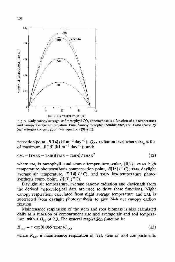
Fig. 5. Daily canopy average leaf mesophyll CO 2 conductance is a function of air temperature and canopy average net radiation. Final canopy mesophyll conductance, CM is also scaled by leaf nitrogen concentration. See equations (9)-(12).

pensation point, B[14] (kJ m - 2 day-a); Q0.5 radiation level where CMq is 0.5 of maximum, B[15] (kJ m - 2 day-a); and:

CM t = ( T M A X -- T A I R ) ( T A I R - - T M I N ) / T M A X 2 (12)

where CM t is mesophyll conductance temperature scalar, {03}; TMXX high temperature photosynthesis compensation point, B[18] ( ° C); TAIR daylight average air temperature, Z[14] (°C) ; and TMIN low-temperature photo- synthesis comp. point, B[17] (o C).

Daylight air temperature, average canopy radiation and daylength from the derived meteorological data are used to drive these functions. Night canopy respiration, calculated from night average temperature and LAI, is subtracted from daylight photosynthesis to give 24-h net canopy carbon fixation.

Maintenance respiration of the stem and root biomass is also calculated daily as a function of compartment size and average air and soil tempera- ture, with a Q10 of 2.3. The general respiration function is:

Rl,s , r = a exp(0.085 T E M P ) Cl,s, r (13)

where R l,s, r is maintenance respiration of leaf, stem or root compartments

139

(kg day- l ) ; a are scaling factors given by B[19], [20], [21] (kg kg-1); 0.085 is a scaling factor that gives a Q10 = 2.34; TEMP night average temperature for leaf respiration, 24-h average temperature for stem respiration, soil tempera- ture for root respiration ( ° C); and CLs,r carbon storage in leaf X[8], or root X[10] compartment, and Cs = exp (0.67 In(X[9])) stem respiration (kg).

The carbon fixation and respiratory losses are accumulated daily, and respiration subtracted from fixation to give a final measure of carbon produced for the year. This carbon is sent to the yearly section of the model and is available for growth.

Yearly submodel

The processes in the yearly submodel covered in this paper are carbon partitioning, growth respiration, litterfall and decomposition. Once per year the available carbon from the daily submodel is partitioned to the leaf, stem and roots.

This allocation is currently defined externally by parameters B[30], [31], [32] (Table 3) based on research results by Keyes and Grier (1981) and Grier

180

160

--~ 100 I~ UGN[N

8o 6o

5~II UGNIN p i i f l i l I I -- ZOO ~I

20 ~0 60 80 100 120 140 160 180

ACTUAL EVAPOTRANSPTRATION (crn year "1}

Fig. 6. Litter decomposition rate is described as a percent weight loss per year, driven by actual annual cvapotranspiration modified by percent l i ~ content of the litter. Simulations in this paper assumed constant ]0% litter [ i ~ n content. See equation (]4).

140

et al. (1981) and models of Mohren et al. (1984) and McMurtr ie and Wolf (1983). Above and below-ground carbon allocation will be treated as a dynamic function of nutrient and water availability in a future version of this model. Growth respiration is subtracted as a fixed fraction of the carbon allocated to each compartment by parameters B[43], [44], [45]. These coefficients are defined from the biochemical energetics of producing carbohydrate, lignin and other complex plant molecules from basic con- stituents, following Mohren et al. (1984) and Penning de Vries et al. (1974). Growth respiration is treated as independent of temperature, assuming that while instantaneous growth rate is temperature-controlled, the annual con- struction costs of biomass are not.

Litterfall or carbon turnover is defined by the coefficients B[40], [41], [42] in this version. A future version of this model will control canopy and root carbon turnover as dynamic functions of water and nutrient availability.

Annual litter decomposition is calculated after Meentemeyer (1984) (Fig. 6) as:

DECOMP = ( - - 3.44 + 0.100 A E T ) - - ((0.0134 + 0.00147 A E T ) L I G ) (14)

where DECOMP is annual percent weight loss of fresh litter (% yea r - l ) ; AET actual annual evapotranspiration, from daily model (ram yea r - l ) ; and LIG initial litter lignin concentration (% dry wt).

Computer code of this model with internal documentat ion, written in Turbo-Pascal for an IBM P C / X T / A T is available from the authors. The simulation of 1 year on an IBM AT takes about 30 s.

SIMULATIONS

A hypothetical stand was defined for the simulations having a LAI = 3, 6 or 9, stem carbon = 50 t / ha , and root carbon = 7.5 t / ha , allocation ratios generalized from Cannell (1985) and Grier et al. (1981). These values are realistic for a relatively mature coniferous forest at all locations except Tucson, which was chosen as an extreme climate where forests survive only in the cooler, wetter mountains above the city. Initial soil water and snowpack conditions were derived by running a preliminary simulation for a year for each site beginning from saturated soil, allowing summer soil moisture depletion and fall snow accumulation to develop, and using the year-end conditions as initial conditions for the formal simulations. Most of the parameters defined in Table 3, BIl l thru B[18], were drawn from an earlier model, documented in Running (1984a, b).

t, metric tonne = 1000 kg.

141

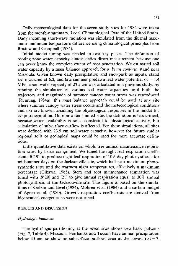
Daily meteorological data for the seven study sites for 1984 were taken from the monthly summary, Local Climatological Data of the United States. Daily incoming short-wave radiation was simulated from the diurnal maxi- m u m - m i n i m u m temperature difference using climatological principles from Bristow and Campbell (1984).

Initial model tuning was needed in two key places. The definition of rooting zone water capacity almost defies direct measurement because one can never know the complete extent of root penetration. We estimated soil water capacity by a mass balance approach for a Pinus contorta stand near Missoula. Given known daily precipitation and snowpack as inputs, stand LAI measured at 6.3, and late summer predawn leaf water potential of - 1 . 4 MPa, a soil water capacity of 23.5 cm was calculated in a previous study, by running the simulation at various soil water capacities until both the trajectory and magnitude of summer canopy water stress was reproduced (Running, 1984a). this mass balance approach could be used at any site where summer canopy water stress occurs and the meteorological conditions and LAI are known, assuming the physiological responses in the model for evapotranspiration. On non-water limited sites the definition is less critical, because water availability is not a constraint to physiological activity, but calculation of subsurface outflow is affected. For these simulations, all sites were defined with 23.5 cm soil water capacity, however for future studies regional soils or geological maps could be used for more accurate defini- tions.

Little quantitative data exists on whole tree annual maintenance respira- tion rates, by tissue component. We tuned the night leaf respiration coeffi- cient, B[19], to produce night leaf respiration of 10% day photosynthesis for midsummer days on the Jacksonville site, which had near maximum photo- synthetic rates and the warmest night temperatures, effectively a maximum percentage (Oikawa, 1985). Stem and root maintenance respiration was tuned with B[20] and [21] to give annual respiration equal to 30% annual photosynthesis at the Jacksonville site. This figure is based on the simula- tions of Golkin and Ewel (1984), Mohren et al. (1984) and a carbon budget of Agren et al. (1980). Growth respiration coefficients are derived from biochemical energetics so were not tuned.

RESULTS AND DISCUSSION

Hydrologic balances

The hydrologic partitioning at the seven sites shows two basic patterns (Fig. 7, Table 4). Missoula, Fairbanks and Tucson have annual precipitation below 40 cm, so show no subsurface outflow, even at the lowest LAI----3.

142

140

1 3 0

120

110

~T 100

~ 9O

l= ~ 0 u

~ 7 0

~ ~ o

1 ~ 0

40

30

2 0

10

J a c k s o n v i l l e K n o x v i l l e

1 4 0

1 3 0

1 1 0

1 0 0 ~ , o

u E ao

70

i , o

3O

1 0

0

J a c k s o n v i l l e K n o x v i l l e

M a d l s o n

M a d i s o n

M l s s o u l a S e c l t f l e

L A I - 3

r a l r b a n k m T u c s o n

1 4 0

1130

1 1 0

* i - 1 O0

,oN ® i " °

3O

10

0

J a c k s o n v i l l e K n o x v i l l e M a d i s a n

OUTFLOW ] ~ "~.] i~VAPORATION

M l l l o u l a S e a t t l e

L A I = 6

r a l r b a n k s T u c s o n

M l s l l o u l a

L A I - 9

S e a t t l e r a l r b a n k s

[ / / / ~ J TRANSPIRATION

T u c s o n

Fig. 7. A comparison of the hydrologic partitioning of annual precipitation between evapora- tion, transpiration and groundwater outflow simulated by FOREST-BGC for 1984 for the seven sites at LAZ = 3, 6, 9. Soil water holding capacity was fixed at 23.5 cm for all simulations.

143

TABLE 4

Annual process rates by FOREST-BGC for the seven study sites at LAI = 3, 6, 9; H20 (cm), C (t/ha).

Jacksonville Knoxville Madison Missoula Seattle Fairbanks Tucson

Initial conditions soil water content 23.0 23.1 23.4 4.5 23.4 15.3 3.6 snowpack 0.0 0.0 12.1 5.3 0.0 6.2 0.0 precipitation 124.4 123.1 80.4 33.7 93.9 31.3 39.4

LAI = 3

Evaporation 11.9 15.2 11.2 8.9 13.3 4.6 8.7 Transpiration 33.3 28.5 20.1 24.5 22.6 16.8 20.4 Outflow 80.6 79.3 57.3 0.0 57.1 0.0 0.0 Canopy net photo-

synthesis 12.5 11.7 8.7 8.6 8.5 7.0 5.6 Maintenance

respiration 6.5 4.5 3.2 2.5 3.0 1.7 7.1 Growth respiration 1.9 2.3 1.9 2.0 1.8 1.7 - 1.5 Net primary

productivity 4.1 4.9 3.6 4.1 3.7 3.6 0.0 leaf 1.0 1.2 0.9 1.0 0.9 0.9 0.0 stem 1.5 1.8 1.3 1.5 1.4 1.3 0.0 root 1.6 1.9 1.4 1.6 1.4 1.4 0.0

Water-use efficiency PSN/transpiration 0.38 0.41 0.43 0.35 0.38 0.42 0.27 yvP/transpiration 0.12 0.17 0.18 0.17 0.16 0.21 0.00

Decomposition rate (%) 35 34 23 25 27 15 21

L A I = 6

Evaporation 17.5 23.4 16.5 11.5 Transpiration 61.9 53.0 37.4 24.5 Outflow 48.1 47.1 34.8 0.0 Canopy net photo-

synthesis 21.2 20.1 14.8 9.9 Maintenance

respiration 6.5 4.5 3.2 2.5 Growth respiration 4.9 5.2 3.8 2.5 Net primary

productivity 9.8 10.4 7.8 4.9 leaf 2.4 2.5 1.9 1.2 stem 3.6 3.8 2.9 1.8 root 3.8 4.1 3.0 1.9

Water-use efficiencies VSN/transpiration 0.34 0.38 0.40 0.40 r4pP/transpiration 0.16 0.20 0.21 0.20

Decomposition rate (%) 64 62 43 27

15.6 5.3 13.1 39.1 30.6 22.5 36.0 0.0 0.0

13.7 11.5 1.5

3.0 1.7 7.1 3.6 3.2 -5 .7

7.1 6.6 0.1 1.7 1.6 0.1 2.6 2.4 0.0 2.8 2.6 0.0

0.35 0.38 0.07 0.18 0.22 0.00

43 27 27

To be continued

144

TABLE 4 (continued)

Jacksonville Knoxville Madison Missoula Seattle Fairbanks Tucson

LAI = 9

Evaporation 17.8 24.8 17.5 11.9 15.6 5.3 14.4 Transpiration 88.7 76.2 50.2 24.4 41.8 33.2 22.5 Outflow 22.9 32.1 24.6 0.0 35.7 0.0 0.0 Canopy net photo-

synthesis 26.9 25.7 18.4 9.9 13.4 12.9 0.0 Maintenance

respiration 6.5 4.5 3.2 2.5 3.0 1.7 7.1 Growth respiration 6.8 7.1 5.0 2.5 3.4 3.7 - 7.1 Net primary

productivity 13.6 14.1 10.2 4.9 7.0 7.5 0.0 leaf 3.3 3.4 2.5 t.2 1.7 1.8 0.0 stem 5.0 5.2 3.7 1.8 2.6 2.8 0.0 root 5.3 5.5 4.0 1.9 2.7 2.9 0.0

Water-use efficiencies VSN/transpiration 0.30 0.34 0.37 0.41 0.32 0.39 0.00 Nvv/transpiration 0.15 0.19 0.20 0.20 0.17 0.23 0.00

Decomposition rate (%) 87 83 54 28 46 29 27

Anderson et al. (1976), in a compilation of forest hydrology research in North America, concluded that water discharge is minimal from forested catchments receiving less than 50 cm year -1 precipitation. On these arid sites, all input is partitioned between evaporation and transpiration by the canopy interception function. Intercepted water evaporates on the day of rainfall, while the remaining water is stored by either snowpack or soil until required for transpiration. The model does limit evaporation to the daily net radiation, the logic being that precipitation beyond this could not be evaporated for lack of latent energy, and would fall off the canopy to the soil. This factor is illustrated in Table 4 where evaporation does not increase linearly with LAI from 3 to 9, as would be predicted from the function in Fig. 3 alone.

The lack of any subsurface outflow at Fairbanks may be overstated, though, because our defined soil water holding capacity of 23.5 cm for all sites is much too generous at Fairbanks, where permafrost is often at 20-40 cm depth (Van Cleve et al., 1983). A soil water capacity of 8 cm would then be more appropriate, and would produce some outflow because the snow- pack peaked at 10 cm water content during the simulation. Both Missoula and Fairbanks have annual hydrologic balances highly influenced by spring snowmelt, the only time of the year where soils can approach saturation. Snowpack is an important water storage for these arid ecosystems, whose

145

plant productivity would be more like Tucson if not for the storage of winter precipitation and efficient transfer of water to soil in the spring.

Hydrologic partitioning at the other four sites is more complicated, where subsurface outflow dominates the balance at an LAI ----- 3, but changes radi- cally with increasing LAI. Anderson et al. (1976) found outflow of 27% and 32% of annual precipitation for two watersheds of pine stands in the Southeastern United States similar to the Jacksonville site. Our simulation results showed outflow of 39% at LAI-----6, and 19% at LAI = 9 for Jack- sonville. Hydrologic outflow was 41% of precipitation for a watershed near Knoxville (Anderson et al., 1976), and the model predicted 38%; and 33% for a watershed near Madison, compared to a prediction of 44%. In Jacksonville, Knoxville and Madison, increasing LAI increased canopy inter- ception and hence evaporation, but also increased transpiration because much of their rain comes during the summer. On these three sites outflow was 19-31% of precipitation at LAI = 9, but increased to 64-71% of precipi- tation at LAI = 3. T h i s pattern of greater outflow at low LAI has been demonstrated repeatedly by increased streamflow of 16-66% after clearcut- ting watersheds in these climates (Anderson et al., 1976, Waring et al., 1981). However in Seattle, evaporation is only weakly influenced, because most of the annual precipitation comes in cold winter storms where lack of latent energy restricts evaporation. Conversely, summer is very dry in this Mediter- ranean climate, so increasing LAI to 6 increased transpiration in Seattle, but further increase to LAI = 9 produced summer canopy water stress and little additional transpiration while outflow stayed unchanged at 38% of precipita- tion.

Missoula also showed no increase in transpiration, from LAI of 3 to 9, because all available soil water is consumed in each case, with an annual precipitation of only 33.7 cm. More LAI produces higher transpiration rates in the spring and then a longer period of canopy water stress in the summer, so seasonal patterns are changed without affecting the total annual budget. We have measured this sensitivity of canopy water stress to LAI in Missoula forests (Donner and Running, 1986). Of course in all these cases the hydrologic partitioning is highly influenced by the soil water holding capac- ity defined, the LAI of the watershed, the annual precipitation, and the periodicity and magnitude of individual precipitation events.

Canopy photosynthesis and transpiration

Figure 8 illustrates the seasonal trends of canopy transpiration and photosynthesis of three sites representing the high and low extremes of temperature and water availability (with the exception of Tucson, an ex- treme site where the model simulated no net primary production). Jack-

146

E E

Z

t A t I'( I : ~A N I~:)

JACKSONVILLE

1 O0 200 300

( a ) Y[AROAY

120

4 0 0

-- 1 O0

ao t.J

so t~

40

zo

0

~ FAIRBAHKS

-- t MISSOULA r i ~ t

100 200 300

( b ) YEAROAY

400

Fig. 8. Seasonal trend of transpiration (a) and photosynthesis (b) simulated by FOREST-BGC for three sites of contrasting climates and growing season lengths for a stand with LAI = 6.

sonville has continuous air temperatures above 0 ° C, year-round precipita- tion and, at a latitude of 30.5 ° C, a seasonal amplitude in daylength of only 10-14 h.

In contrast to the year-round growing season of Jacksonville, Fairbanks has temperatures above freezing only for the period of yearday 100-280, but

147

during mid-summer at 65 deg latitude daylength extends to 22 h, producing the highest daily photosynthesis and transpiration in the model runs. How- ever again, we feel these generic model runs to be weakest for Fairbanks. Transpiration is known to be reduced by low soil temperatures, yet the meteorological data did not include soil temperature, and the derived soil temperature in the model is too strongly influenced by air temperature. A site with permafrost at 40 cm never has soil temperatures above 5 o C, yet the model may predict 10 °C resulting in no computed restriction of physiologi- cal activity. As stated in the hydrology section, the soil water holding capacity at Fairbanks should probably be around 8 cm, which would cause summer canopy water stress, reducing transpiration and photosynthesis.

Photosynthesis is probably overestimated at Fairbanks for two additional reasons. First, it has been widely demonstrated that leaves recovering from severe winter temperatures require 2-4 weeks to rebuild photosynthetic biochemistry and reach maximum photosynthetic potential, a lag period the model does not treat (Tranquillini, 1979; Linder, 1981). Secondly, these general simulations were done with a leaf nitrogen concentration of 1.5%, but boreal forests are known to be particularly nitrogen limited so these simulations may represent only the best forests on warm, fertile south exposures, not average conditions (Van Cleve et al., 1983).

The seasonal trends for Missoula illustrate the effect of substantial canopy water stress on gas exchange. Both transpiration and photosynthesis dropped almost to zero around yearday 200 in response to a calculated predawn leaf water potential of - 1 .7 MPa, very similar to measured values (Running, 1984a; Graham and Running 1984). Late summer and fall rains allowed some recovery in gas exchange, but by yearday 280 low air temper- atures and shorter daylengths bring activity to a stop.

It is often implied that photosynthesis is directly related to transpiration, and in this model they are linked through the cc or canopy conductance term. However, radiation drives photosynthesis strongly (Fig. 5) while being a much weaker component of the transpiration driver in the Penman-Mon- teith equation (8). Also, absolute humidity deficit directly drives transpira- tion yet has no effect on the driving force of photosynthesis, and has only a weak feedback control through the cc term in equation (9). To explore the degree of correlation across different climates, we regressed weekly tran- spiration against weekly photosynthesis for all sites. In some climates photosynthesis and transpiration were highly correlated, in Fairbanks R 2 --- 0.96, in Seattle, R 2 = 0.95; but in Jacksonville R 2 = 0.40, and in Knoxville, R 2= 0.79. Inspecting the seasonal trends on all sites (not shown), dis- crepancies were highest in the spring at sites like Seattle, where clear but cool days allowed high photosynthesis but at relatively low transpiration because of low vapor pressure deficits, and summer in Jacksonville and

148

Z

0

28

2 4

22

20

18

, 6 ~¢J 1 4

~° ~ 8

4

2

0

J a c k s o n v i l l e K n o x v i l l e M a d i s o n M l s s o u l a S e a t t l e F a l r b a n k s

H T u c s o n

LAI ~ 2~ ~ LAI = 6 ~ LAI m 9

Fig. 9. Response of seasonal canopy net photosynthesis simulated by F O R E S T - B G C for seven sites of contrasting climate for LAI = 3, 6, 9.

Knoxville, where hot but cloudy days allowed high transpiration but at relatively lower light-limited photosynthesis.

The response of increasing LAI on annual canopy photosynthesis was quite variable in the different climates (Fig. 9). On sites of moderate temperature extremes and adequate water availability, such as Jacksonville and Knoxville, increasing LAI increased annual photosynthesis proportion- ally. However, on sites where physiological activity is substantially water- limited (Missoula, Tucson) or radiation-limited (Seattle), increasing LAI produced either a weak positive or even negative response in photosynthesis (Fig. 9). High LAI can be a detriment in climates with high maintenance respiration costs, a consequence of high night temperature (Oikawa, 1985). Adding LAI on severely water-limited sites merely extended the period of severe canopy water stress, shown in Fig. 8 for Missoula. Photosynthesis increased by 60% between LAIS of 3 and 6 in Fairbanks, but at LAI ----" 9 water stress restricted additional gains. Grier and Running (1977) measured a transect of mature conifer forests in Oregon, and found LAI ranging from 1 t o 15 m 2 m -2 were correlated with an annual site water balance, R 2 = 0.99. Gholz (1982) also measured a very high correlation between site water availability and both LAI and annual net primary production of coniferous forests across Oregon.

At Seattle photosynthesis actually decreased as LAI increased from 6 to 9 for two reasons. Despite the high annual precipitation, Seattle experiences

149

extended drought in late summer, so higher LAI accelerates that drought period. Also, winters in Seattle are above freezing yet with very short daylengths and low radiation due to the fog and clouds of this coastal environment. Consequently the wintertime respiration load of additional LAI may not be compensated sufficiently by higher photosynthesis. However, Graham and Running (1985) also made photosynthesis simulations using Seattle climatological data and concluded that the low winter radiation totals recorded are somewhat an artifact of the location of the meteorologi- cal bureau in a fog pocket, and underestimates the radiation received by the general region. Also, these generic simulations did not include seasonal shifts in temperature or radiation optima for photosynthesis, factors that have been suggested to allow substantial wintertime carbon fixation in Pacific Northwest forests (Waring and Schlesinger, 1985).

Water use efficiency as defined by PSN/TRAN (t C ha-1 (mm n 2 0 ) - 1 was highest on all sites at LAI = 3 , because the highest proportion of canopy was at light saturation (Table 4). Water-use efficiency ranged from 0.30 to 0.43 t C ha -~ (mm H20) -1 across sites and LkI with no real trend evident. Despite theoretical arguments that water-use efficiency increases at higher humidity, that trend was not evident from these ratios of annual sums of PSN and TRAN. Water-use efficiency in the model is influenced by the ratio of maximum canopy conductance/maximum mesophyll conductance, or B[ll]/B[16]. The ratio of 0.0016/0.0008 m s - 1 = 2.0 was used for these simulations (Jarvis, 1981), however the ratio of actual conductances changes daily with the meteorological controls of the conductances shown in Figs. 4 and 5.

Net primary production-respiration

Simulated NPP ranged from 0.0 at Tucson to 14.1 t C ha -~ year -1 at Knoxville with LgI = 9 (Table 4), a range of NaP quite similar to that found for forests around the U.S. of 3.5-15 t C ha -1 year -1 by Webb et al. (1983). Gholz (1986) in analyzing aboveground NPP of 78 forest stands reported in the literature found a range from 0.5 to 13.6 t C with a mean of 5.5 t C ha -1 year -1. Assuming 40% belowground NPP, an average total NaP = 7.6 t C ha -1 year -~ is found, in the center of our range of calculated NPP. For reasons previously stated, Fairbanks had higher NPP than expected, 6.6 t C at LAI = 6. However, Yarie and Van Cleve (1983) report aboveground NPP of 1-15 t dry weight per year on good Picea glauca stands, and our estimate, translated to aboveground dry weight is 8.8 t year -~ at LAI ~-~ 6 , and 10.1 t year -~ at LAI = 9 , well within the range reported. NPP at Seattle was calculated at 7.1 t C or 15.6 t dry wt ha -1 year -1 at LAI = 6. Grier et al.

150

(1981) and Keyes and Grier (1981) report total Nel' of 15.4 -- 18.3 t dry wt ha -1 year -1 including above and below-ground production for four sites near Seattle, a reasonable correspondence. Kinerson et al. (1977) reported total Nl, e of 20.56 t C ha -1 year -1 for a Pinus taeda plantation, consider- ably higher than our maximum yap of 14.1, but that NPP is the highest ever recorded. Gholz and Fisher (1982) report aboveground NPP of 12 MT for a Pinus elliottii stand with tAX = 6.5. Our calculated above-ground NaP esti- mate for Jacksonville at LAX = 6 is 6.0 t C, or 13.2 t dry wt ha -1 year -1. Generally, our estimates of NPP seem accurate both in a relative sense across sites and climates, and in an absolute sense, when compared to field measurements.

In contrast to net primary production estimates, where a wealth of field data is available to test the model, there are few annual respiration data for forests. Landsberg (1986) generalized from a variety of sources that total respiration losses from branches, stems and roots of trees ranges from 25 to 50% of annual net photosynthesis. In the FOREST-BGC model, growth respiration is a fixed proportion of the carbon available for growth (see B[43], [44], and [45] in Table 3), and is not controlled by climate, so is a constant proportion across sites. Maintenance respiration is driven exponen- tially by air temperature with a Q~0 = 2.3, so warmer sites showed higher annual maintenance respiration. For LAI = 6, Jacksonville, had maintenance respiration equal to 31% of annual net photosynthesis , while Fairbanks was 15% of photosynthesis, with other sites being between these extremes (Table 4). Because we calculated negative carbon balances for the Tucson site, we are not interpreting that data.

Probably the most comprehensive analysis of the respiration component of tree carbon budgets is the analysis by Waring and Schlesinger (1985), of work by Kinerson et al. (1977) and Linder and Troeng (1981). Kinerson et al. (1977) found maintenance respiration to be 32% and growth respiration to be 15% of annual photosynthesis for a P. taeda stand in North Carolina. Our most comparable site would be Knoxville at LAI = 6, where mainte- nance respiration was 22% and growth respiration was 26%. Likewise, Linder and Troeng (1981) found maintenance respiration at 11%, and growth respiration at 20% of annual photosynthesis for a P. syloestris tree in Sweden. Our Fairbanks site showed at LAI = 6, maintenance respiration of 15% and growth respiration of 28% of annual photosynthesis. Tranquillini (1979) reported stem respiration of 16.9-23.1% of annual net photosynthesis for two conifers at timberline in the Austrian alps. Given that these model runs were based on general forest biomass estimates not tuned for any particular site we are satisfied with the basic correspondence in both relative and absolute magnitude of these respiration calculations to the rather sparse data available.

151

Decomposition

For the LAI = 6 simulations, decomposition annual weight losses, ranged from 27% at Fairbanks to 64% at Jacksonville (Table 4). These figures correspond with those of Meentemeyer (1984), who estimated 20% for Alaska and 70% for Florida for litter with 15% lignin content. However, Vogt et al. (1986) report a wide range of litter decomposition rates, and suggest that particularly in the tropics, lignin content controls decomposi- tion rates more strongly than climate. We see lignin control of decomposi- tion as another critical point where general simulations must be para- meterized by local data.

Actual evapotranspiration (A~T) increased on many of our sites as LAI increased from 3 to 9, most dramatically at the non-water-limited sites of Jacksonville and Knoxville. Increased AET caused the decomposition rate to increase from 35 to 87% at Jacksonville, using the AET driven decomposition equation of Meentemeyer (1984). However, higher LAI reduces radiation to the litter surface, decreasing soil temperatures, and increases canopy inter- ception, reducing litter moisture content, both factors which should slow decomposition rates. Consequently, we feel that the results at different LAI are not legitimate, and consider the decomposition estimates to be reasona- ble only for relative comparisons across sites at a fixed LAI.

CONCLUSIONS

We conclude that FOREST-BGC can represent relative differences in basic ecosystem processes of forests in contrasting climates at continental scales when run in a general mode, without site or species-specific tuning. The relative ranking of hydrologic balances, and annual net primary produc- tion across sites of widely varying climate agrees with general estimates of these processes in each region. More specific calculations of canopy gas exchange rates, respiration and decomposition rates will require more local parameter estimation to provide discrimination of site and stand differences at local scales. A more satisfactory validation of the model should include measurement of specific parameters and site meteorological data on specific forest stands across this climatic range, with independently measured processes to compare with model calculations, a rather major undertaking.

We also conclude that accurate parameterization of LAI for different sites will improve model estimations, because these results show substantial and differential effects of LAI on ecosystem processes in contrasting climates. The potential of satellite data to map LAI of forest over large areas is thus important for regional simulations of ecosystem processes. FOREST-BGC has already been used to analyze and interpret the seasonal trends of a

152

satellite derived weekly global vegetation index (Running and Nemani, 1988). The integrated annual global vegetation index for 1984 was correlated with annual photosynthesis, R 2 = 0.87, transpiration, R z= 0.77, and net primary production, R 2= 0.72, simulated by FOREST-BGC for the seven sites in this paper, providing strong evidence of a relationship between satellite data and vegetation process rates (Running and Nemani, 1988).

ACKNOWLEDGEMENTS

This research was funded by Joint Research Interchanges NCA 2-27 and NCA 2-252 with the NASA Ames Research Center, Moffett Field, CA. We thank Ross McMurtrie, Trevor Booth, Ray Leuning, Bill Thompson and David L. Peterson for critical review of the draft manuscript. John Aber, Pam Matson and Peter Vitousek were instrumental in helping design the model structure. This research was completed while the senior author was a visiting scientist at the CSIRO Division of Forest Research, Canberra, Australia.

REFERENCES

Agren, G.I., Axelsson, B., Flower-Ellis, J.G.K., Linder, S., Persson, H., Staff, H. and Troeng, E., 1980. Annual carbon budget for a young Scots pine. In: T. Persson (Editor), Structure and Function of Northern Coniferous Forests-An Ecosystem Study. Ecol. Bull. NFR, 32: 307-313.

Anderson, H.W., Hoover, M.D. and Reinhart, K.G., 1976. Forests and water: effects of forest management on floods, sedimentation and water supply. USDA For. Sere. Gen. Tech. Rep. PSW-18, 115 pp.

Asrar, G., Fuchs, M., Kanemasu, E.T. and Hatfield, J.L., 1984. Estimating absorbed photo- synthetic radiation and leaf area index from spectral reflectance in wheat. Agron. J., 76: 300-306.

Botkin, D.B. (Chair), 1986. Remote sensing of the biosphere. Report of the Committee on Planetary Biology. National Research Council, National Academy of Sciences, New York.

Bristow, K.L. and Campbell, G.S., 1984. On the relationship between incoming solar radiation and daily maximum and minimum temperature. Agric. For. Meteorol., 31: 159-166.

Cannell, M.G.R., 1985. Dry matter partitioning in tree crops. In: M.G.R. Cannell and J.E. Jackson (Editors). Attributes of Trees as Crop Plants. Institute of Terrestrial Ecology, Midlothian, Great Britain.

Donner, B.L. and Running, S.W., 1986. Water stress response after thinning Pinus contorta stands in Montana. For. Sci., 32: 614-625.

Gamier, B.J. and Ohmura, A., 1968. A method of calculating the direct shortwave radiation income of slopes. J. Appl. Meteorol., 7: 796-800.

Gholz, H.L., 1982. Environmental limits on aboveground net primary production, leaf area, and biomass in vegetation zones of the Pacific Northwest. Ecology, 63: 469-481.

Gholz, H.L., 1986. Canopy development and dynamics in relation to primary production. In: Crown and Canopy Structure in Relation to Productivity. IUFRO Proc. Forestry and Forest Products Research Institute, Ibaraki, Japan, pp. 224-242.

153

Gholz, H.L. and Fisher, R.F., 1982. Organic matter production and distribution in slash pine (Pinus elliottii) plantations. Ecology, 63: 1827-1839.

Golkin, K. and Ewel, K.C., 1984. A computer simulation of the carbon, phosphorus, and hydrologic cycles of a pine flatwoods ecosystem. Ecol. Modelling, 24: 113-136.

Graham, J.S. and Running, S.W., 1984. Relative control of air temperature and water status on seasonal transpiration of Pinus contorta. Can. J. For, Res., 14: 833-838.

Graham, R.L., Farnum, P., Timmis, R. and Ritchie, G., 1985. Using modelling as a tool to increase forest productivity and value. In: 4th Weyerhaueser Science Symposium, Tacoma, WA, pp. 101-130.

Grier, C.C. and Running, S.W., 1977. Leaf area of mature northwestern coniferous forests: relation to site water balance. Ecology, 58: 893-899.

Grief, C.C., Vogt, K.A., Keyes, M.R. and Edmonds, R.L., 1981. Biomass distribution and above- and below-ground production in young and mature Abies amabilis zone ecosystems of the Washington Cascades. Can. J. For. Res., 11: 155-167.

Jarvis, P.G., 1981. Production efficiency of coniferous forest in the UK. In: Physiological processes controlling plant productivity. C.B. Johnson (Editor), Butterworths, London, pp. 81-107.

Keyes, M.R. and Grier, C.C., 1981. Above- and below-ground net production in 40-year-old Douglas-fir stands on high and low productivity sites. Can. J. For. Res., 11: 599-605.

Kinerson, R.S., Ralston, C.W. and Wells, C.G., 1977. Carbon cycling in a loblolly pine plantation. Oecologia, 29: 1-10.

Landsberg, J.J., 1986. Physiological ecology of forest production. Academic Press, London, 198 pp.

Linder, S., 1981. Understanding and predicting tree growth. Stud. For. Suec. 160, 87 pp. Linder, S. and Troeng, E., 1981. The seasonal variation in stem and coarse root respiration of

a 20-year-old Scots pine (Pinus syloestris L.). Mitt. Forstl. Bundus Versuchanst. Wien. Lohammar, T., Larsson, S., Linder, S. and Falk, S.O., 1980. FAST-Simulation models of

gaseous exchange in Scots pine. In: (T. Persson (Editor), Structure and Function of Northern Coniferous Forests-An Ecosystem Study. Ecol. Bull., 32: 505-523.

McMurtrie, R., and Wolf, L., 1983. Above and below-ground growth of forest stands: a carbon budget model. Ann. Bot., 52: 437-448.

Meentemeyer, V., 1984. The geography of organic decomposition rates. Ann. Assoc. Am. Geogr., 74: 551-560.

Mohren, G.M.J., Van Gerwen, C.P. and Spitters, C.J.T., 1984. Simulation of primary production in even-aged stands of Douglas fir. For. Ecol. Manage., 9: 27-49.

Murray, F.W., 1967. On the computation of saturation vapor pressure. J. Appl. Meteorol., 6: 203-204.

Oikawa, T. 1985. Simulation of forest carbon dynamics based on a dry-matter production model. I. Fundamental model structure of a tropical rainforest ecosystem. Bot. Mag. Tokyo, 98: 225-238.

Penning de Vries, F.W.T., Brunsting, A. and Van Laar, H.H., 1974. Products, requirements and efficiency of biosynthesis; a quantitative approach. J. Theor. Biol., 45: 339-377.

Peterson, D.L., Matson, P.A., Lawless, J.G., Aber, J.D., Vitousek, P.M. and Running, S.W., 1985. Biogeochemical cycling in terrestrial ecosystems: modeling, measurement, and remote sensing. In: Proc. 36th Int. Astronautical Fed. Congr., Stockholm, Sweden.

Running, S.W., 1984a. Microclimate control of forest productivity: Analysis by computer simulation of annual photosynthesis/transpiration balance in different environments. Agric. For. Meteorol., 32: 267-288.

Running, S.W., 1984b. Documentation and prelimary validation of H2OTRANS and

154

DAYTRANS, two models for predicting transpiration and water stress in western conifer- ous forests. USDA For. Serv. Rocky Mount. For. Range Exp. Stn. Res. Pap. RM-252, 45 pP.

Running, S.W. and Nemani, R.R., 1988. Relating seasonal patterns of the AVHRR Vegeta- tion Index to simulated photosynthesis and transpiration of forest in different climates. Remote Sensing Environ., 24: 347-367.

Running, S.W., Peterson, D.L., Spanner, M.A. and Teuber, K.B., 1986. Remote sensing of coniferous forest leaf area. Ecology, 67: 273-276.

Running, S.W., Nemani, R.R. and Hungerford, R.D., 1987. Extrapolation of synoptic meteorological data in mountainous terrain, and its use for simulating forest evapotranspiration and photosynthesis. Can. J. For. Res., 17: 472-483.

Tranquillini, W., 1979. Physiological ecology of the alpine timberline. Ecological Studies, 31. Springer, New York.

Van Cleve, K.L., Oliver, L., Schlentner, R., Viereck, L. and Dyrness, C.T., 1983. Productivity and nutrient cycling in tiaga forest exosystems. Can. J. For. Res., 13: 747-766.

Vogt, K.A., Grier, C.C. and Vogt, D.J., 1986. Production, turnover, and nutrient dynamics of above-and belowground detritus of world forests. Adv. Ecol. Res., 15: 303-377.

Waring, R.H. and Schlesinger, W.H., 1985. Forest Ecosystems: Concepts and Management. Academic Press, Orlando, FL, 340 pp.

Waring, R.H., Rogers, J.J. and Swank, W.T., 1981. Water relations and hydrologic cycles. In: D.E. Reichle (Editor), Dynamic Properties of Forest Ecosystems. Cambridge University Press, New York.

Webb, W.L., Lauenroth, W.K., Szarek, S.R. and Kinerson, R.S., 1983. Primary production and abiotic controls in forests, grasslands and desert ecosystems in the United States. Ecology, 64: 134-151.

Wittwer, S. (Chair), 1983. Land related global habitability science issues. NASA Tech. Mem. 85841, 112 pp.

Yarie, J. and Van Cleve, K., 1983. Biomass and productivity of white spruce stands in interior Alaska. Can. J. For. Res., 13: 767-772.

Yates, H., Strong, A., McGinnis, D. and Tarpley, D., 1986. Terrestrial observations from NOAA operational satellites. Science, 231: 463-470.